Obstacle Detection of Intelligent Vehicle Based on Fusion ...

Abstract—Obstacle detection is the key technology of

environment perception for intelligent vehicle. To guarantee

safe operation of an unmanned vehicle the fusion method of

spatial information from lidar and machine vision is studied.

The projection of the bounding box generated by lidar on

machine vision image is designed. The detection area of obstacle

is constructed. Moreover, the method of strong-classifier

cascade connection is used to build a classifier. Specially, the

Haar-like and HOG features within a huge amount of data are

characterized based on AdaBoost algorithm. To achieve

classification and recognition of the obstacles, the obstacle

detection areas generated on the image are fused with the

designed cascade classifier, and the effectiveness of the

proposed fusion method is validated. Test results show that the

obstacle detection method based on fusion of laser radar and

machine vision shows higher detection accuracy. Under good

weather conditions, compared with the detection method based

on laser radar alone and based on machine vision alone, the

proposed method increases the detection rate of vehicle obstacle

by 18.33% and 12.74%, and increase the detection rate of

pedestrian by 17.92% and 12.56%, respectively. Under the

rainy weather, the detection rate of vehicle obstacle is improved

by 38.44% and 14.28%, and the detection rate of pedestrian is

enhanced by 29.34% and 15.84%, respectively.

Index Terms—unmanned vehicle, obstacle detection, data

fusion, laser radar, machine vision

I. INTRODUCTION

utonomous drive technology of intelligent vehicle

involves environment perception, path planning,

intelligent decision and motion control [1-3]. Among them,

environment perception is to obtain surrounding environment

Manuscript received October 26, 2020; revised March 26, 2021. This

work was supported in part by the National Natural Science Foundation of

China under Grant 51805301, the Natural Science Foundation of Shandong under Grant ZR2019BEE043, the Postdoctoral Science Foundation of China

and Shandong under Grant 2020M680091 and 202003042, the key R & D projects in Shandong under Grant 2019GHZ016.

Binbin Sun, is professor of School of Transportation and Vehicle

Engineering, Shandong University of Technology, Zibo, China (e-mail: [email protected]).

Wentao Li, the corresponding author, is graduate student of School of Transportation and Vehicle Engineering, Shandong University of

Technology, Zibo, China (e-mail: [email protected]).

Huibin Liu, is graduate student of School of Transportation and Vehicle Engineering, Shandong University of Technology, Zibo, China (e-mail:

[email protected]).

Jinghao Yan, is graduate student of School of Transportation and Vehicle

Engineering, Shandong University of Technology, Zibo, China (e-mail:

[email protected]). Song Gao, is professor of School of Transportation and Vehicle

Engineering, Shandong University of Technology, Zibo, China (e-mail: [email protected]).

Penghang Feng, is graduate student of School of Transportation and

Vehicle Engineering, Shandong University of Technology, Zibo, China (e-mail: [email protected]).

information of the vehicle through the on-board sensors, and

then identify obstacles based on fusion of multi-source data,

As a pre-condition for path planning, intelligent decision and

motion control the environment perception is essential for the

development of intelligent vehicle [4].

At present, three common modes are utilized to achieve

environment perception for obstacle detection, including

machine vision, millimeter-wave radar and data fusion of

multiple sensors [5]. Data collected by camera affects

machine vision-based obstacle detection results. The obstacle

detection method based on machine vision has advantages of

large detection range and perfect target information.

However, it cannot obtain depth information [6].

Millimeter-wave radar has advantages of high resolution,

high robustness to weather influence, and real-time feedback

on relative position, speed and distance. However, the noise

of such technology is too large to generate obstacle contour

[7]. Under good weather conditions, lidar-based detection

method of obstacle obtains a large amount of

three-dimensional information of the environment directly,

with small data noise and high measurement accuracy.

However, the detection performance of such method is

significantly decreased under bad weather [8].

Generally, a single sensor is inadequate to obtain sufficient

driving environment information. Therefore, obstacle

detection based on fusion of the information collected from

dual or multi-sensors is designed. This advanced technology

makes full use of multiple sensors, so it has improved

perception accuracy and reliability [9]. Currently, data fusion

between different kind of sensors has been commonly

applied in practice, such as data fusion between millimeter

wave radar and machine vision, data fusion between laser

radar and machine vision, and so on [10].

As for obstacle detection based on fusion of millimeter

wave radar and machine vision, the information about

distance and angle of obstacle is confirmed by millimeter

wave radar, and the obstacle recognition is realized via

machine vision. However, such obstacle detection method

shows high false warning rate and large missing rate target

detection [11]. The obstacle detection method based on dual

or triple machine visions uses the stereo camera to obtain the

scale and contour data simultaneously, identifies the obstacle

by V view, but fails to obtain depth information for path

planning and intelligent decision making [12-13]. In contrast,

using the obstacle detection method based on fusion of lidar

and machine vision, the location of obstacle can be obtained

by radar, and then the obstacle can be identified by image

vision processing and classifier [14-15], so more accurate and

comprehensive information can be obtained. However, the

perception accuracy and real-time performance of the

proposed method remain to be further improved due to the

Obstacle Detection of Intelligent Vehicle Based

on Fusion of Lidar and Machine Vision

Binbin Sun, Wentao Li, Huibin Liu, Jinghao Yan, Song Gao and Penghang Feng

A

Engineering Letters, 29:2, EL_29_2_41

Volume 29, Issue 2: June 2021

______________________________________________________________________________________

javascript:;

low processing speed of input data [15-16].

To this end, a dual-sensors fusion method based on a 3-D

32-line lidar and a monocular camera is proposed in this

paper. By creating the area of interest for obstacle detection,

it is possible to realize the extraction of Haar-like and HOG

features, the design of cascade classifier, and obstacle

detection in a real time manner. Specially, in chapter 1, the

conversion of coordinate systems of laser radar and machine

sensor is completed, and the projection method of bounding

box generated by laser radar on machine vision image is

proposed to construct obstacle detection area of interest. In

Chapter 2, the method based on Haar-like and HOG features

is designed to calculate the characteristic value of obstacle,

and a cascaded classifier is created to detect obstacle. Chapter

3 presents details about test and data discussion.

II. OBSTACLE DETECTION REGION OF INTEREST

A. Fusion of Spatial Information from Laser Radar and

Machine Vision

Four coordinate systems are designed in the machine

vision system, including world coordinate system, camera

coordinate system, imaging plane coordinate system and

image pixel coordinate system. In this paper, the first one is

defined as the body coordinate of the intelligent vehicle

installed with camera. The camera coordinate system is

created based on its center. The imaging plane and the pixel

coordinate systems use physical and pixel units as

benchmarks, respectively. There are two conversions of

coordinate systems regarding the fusion of spatial

information of lidar and machine vision. One is the

three-dimensional transformation from world coordinate

system to camera coordinate system. The other one is the

conversion from camera coordinate system to pixel

coordinate system. The transformation uses imaging plane

coordinate system is used as an intermediate medium to

realize the conversion form three-dimension to

two-dimension.

Conversion from World Coordinate System to Camera

Coordinate System

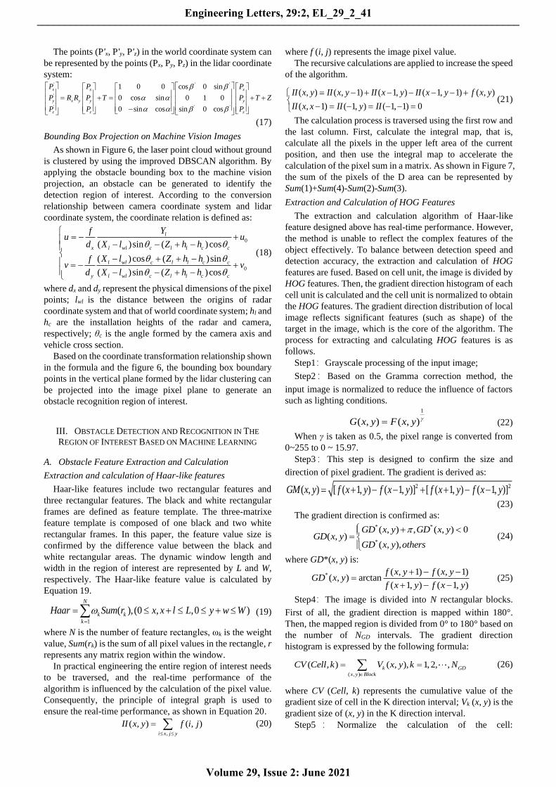
As shown in Figure 1, world and camera coordinates are

illustrated. They are represented by O-XwYwZw and

O-XcamYcamZcam, respectively. The transformation relationship

between the two coordinates belongs to the Euclidean

transformation, that is, one has rotation matrix R and the

other one has translation vector T.

Therefore, for the same data in world coordinate and

camera coordinate, the conversion is confirmed by the

following formula.

cam w

cam w

cam w

x x

y R y T

z z

= +

(1)

The rotation matrix R is related to the installation position

of camera, the heading angle φ, pitch angle δ, and roll angle ξ.

T is determined by the camera installation position.

cos cos sin cos sin

sin cos cos sin cos cos cos sin sin sin cos sin

sin sin cos sin cos cos cos sin sin cos cos cos

R

−

= − + + + − +

(2)

Fig. 1. The conversion from world coordinate system to camera coordinate

system

Conversion from Camera Coordinate System to Pixel

Coordinate System

Figure 2 shows the schematic of the camera aperture. Point

O and o1 represent the center of camera coordinate and the

intersection of axis z and imaging plane, respectively. The

distance between the two points is defined as f. The imaging

and pixel coordinate systems are represented by o1-xcyc and

o1-uv, respectively. Furthermore, point Q is projected to q

from three-dimensional space to imaging plane. According to

the triangular proportional relationship, the relationship is

expressed as:

Xx f

Z= (3)

Yy f

Z= (4)

As shown in formula 5 and 6, the transformation

relationship from point Q to point q can be expressed as

q=MQ.

0 0

, 0 0 ,

0 0 1

xZ f X

q yZ M f Q Y

Z Z

= = =

(5)

Given the above analysis, the relationship between camera

coordinate system and imaging plane coordinate system is

expressed as:

0 0

0 0

0 0 1

x f X

Z y f Y

z Z

=

(6)

Fig. 2. Schematic of small-hole imaging model



______________________________________________________________________________________

In pixel plane, the size of each pixel is the product of dx

and dy. Based on the following relationship, point q is

converted from imaging plane coordinate system to pixel

coordinate system.

0

x

xu u

d= + (7)

0

y

yv v

d= + (8)

Based on the above analysis, the data fusion of imaging

plane coordinate system and pixel coordinate system is

realized.

0

0

0

0

10 0 1

x

y

fu

du X X

fZ v K Y v Y

dZ Z

= =

(9)

B. Detection Region of Interest Based on Data Fusion

Conversion from Lidar Coordinate System to World

Coordinate System

In this paper, world coordinate system (Ow-XwYwZw) is

used to characterize the coordinate of vehicle body. The

centroid point of the vehicle is located on the origin of world

coordinate system. Two coordinate systems are designed for

lidar: one is the reference coordinate system (Olb-XlbYlbZlb)

and the other one is the actual coordinate system

(Olr-XlrYlrZlr). As shown in Figure 3, the two coordinate

systems have different locations on axis Z. Therefore, the

relationship of lidar and the vehicle body is confirmed by R

and T. '

'

1

+

x x

y y

zz

P P

P R P T Z

PP

= +

(10)

where, Z and T are the translation vectors. Since the two

origins discussed above are on the same axis z, T is defined as

[tx, ty, tz]T.

Fig. 3. The world coordinate, lidar reference coordinate and actual

coordinate

During the installation process of lidar, the deviations of

roll angle, pitch angle and deflection angle are unavoidable.

The error of R will directly determine the error of the final

return value of radar, so it is necessary to calibrate the radar

accurately. In this study, the pitch angle is α, the roll angle is

β'，and the deflection angle is γ'. Since the radar is installed

in the center of the longitudinal vertical plane of the vehicle

body, only the calibration of α and β' is required:

As shown in Figure 4, a rectangular calibration plate is

used to calibrate the roll angle of lidar.

The ∠FOE in Figure 4 is the azimuth difference between

the edge points E and F of the radar and rectangular

calibration plate. lOE, lOF represent the distance between point

E and radar as well as that between the point F and radar,

respectively. lEF can be obtained according to the cosine

theorem, then the roll angle β' can be expressed by Equation

11:

' = arccos( )AB

EF

l

l (11)

Fig. 4. The calibration of Lidar roll angle

The roll angle transformation matrix Ry of the radar is

shown in Equation 12: ' '

' '

cos 0 sin

0 1 0

sin 0 cos

yR

=

(12)

The pitch angle is calibrated by using an isosceles triangle

calibration plate. As shown in Figure 5. the triangular

calibration plate is placed at A1, and ∠F1OE1, lOE1, and lOF1

can all be acquired by radar data. Similarly, lEF1 can be

obtained according to the cosine theorem.

1 1 1 1

'cosE Z E Fl l = (13)

1 1 1BZ BC E Zl l l= − (14)

By moving the triangle calibration plate to A2, lBZ2 can be

obtained in the same way, and then the available radar

elevation angle can be calculated as follow:

1 2

1 2

= arctan( )BZ BZ

A A

l l

l

− (15)

The transformation matrix Rx is:

1 0 0

0 cos sin

0 sin cos

xR

= −

(16)

Fig. 5. The calibration of Lidar pitch angle



______________________________________________________________________________________

The points (P'x, P'y, P'z) in the world coordinate system can

be represented by the points (Px, Py, Pz) in the lidar coordinate

system: ' ' '

'

' ' '

1 0 0 cos 0 sin

0 cos sin 0 1 0

0 sin cos sin 0 cos

x x x

y x y y y

z z z

P P P

P R R P T P T Z

P P P

= + = + + −

(17)

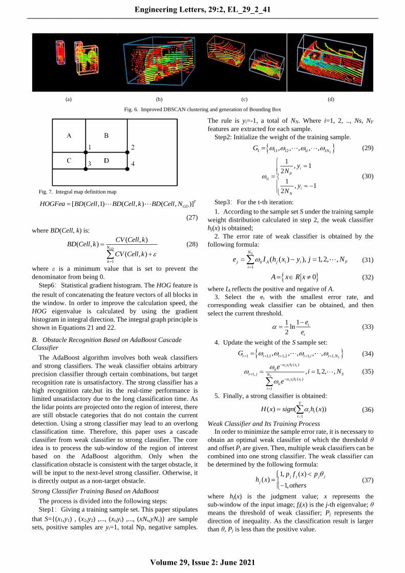
Bounding Box Projection on Machine Vision Images

As shown in Figure 6, the laser point cloud without ground

is clustered by using the improved DBSCAN algorithm. By

applying the obstacle bounding box to the machine vision

projection, an obstacle can be generated to identify the

detection region of interest. According to the conversion

relationship between camera coordinate system and lidar

coordinate system, the coordinate relation is defined as:

0

0

( )sin ( )cos

( )cos ( )sin

( )sin ( )cos

l

x l wl c l l c c

l wl c l l c c

y l wl c l l c c

Yfu u

d X l Z h h

X l Z h hfv v

d X l Z h h

= − + − − + −

− + + − = − +

− − + −

(18)

where dx and dy represent the physical dimensions of the pixel

points; lwl is the distance between the origins of radar

coordinate system and that of world coordinate system; hl and

hc are the installation heights of the radar and camera,

respectively; θc is the angle formed by the camera axis and

vehicle cross section.

Based on the coordinate transformation relationship shown

in the formula and the figure 6, the bounding box boundary

points in the vertical plane formed by the lidar clustering can

be projected into the image pixel plane to generate an

obstacle recognition region of interest.

III. OBSTACLE DETECTION AND RECOGNITION IN THE

REGION OF INTEREST BASED ON MACHINE LEARNING

A. Obstacle Feature Extraction and Calculation

Extraction and calculation of Haar-like features

Haar-like features include two rectangular features and

three rectangular features. The black and white rectangular

frames are defined as feature template. The three-matrixe

feature template is composed of one black and two white

rectangular frames. In this paper, the feature value size is

confirmed by the difference value between the black and

white rectangular areas. The dynamic window length and

width in the region of interest are represented by L and W,

respectively. The Haar-like feature value is calculated by

Equation 19.

1

( ), (0 , ,0 )N

k k

k

Haar Sum r x x l L y w W=

= + + (19)

where N is the number of feature rectangles, ωk is the weight

value, Sum(rk) is the sum of all pixel values in the rectangle, r

represents any matrix region within the window.

In practical engineering the entire region of interest needs

to be traversed, and the real-time performance of the

algorithm is influenced by the calculation of the pixel value.

Consequently, the principle of integral graph is used to

ensure the real-time performance, as shown in Equation 20.

,

( , ) ( , )i x j y

II x y f i j

= (20)

where f (i, j) represents the image pixel value.

The recursive calculations are applied to increase the speed

of the algorithm.

( , ) ( , 1) ( 1, ) ( 1, 1) ( , )

( , 1) ( 1, ) ( 1, 1) 0

II x y II x y II x y II x y f x y

II x x II y II

= − + − − − − +

− = − = − − =(21)

The calculation process is traversed using the first row and

the last column. First, calculate the integral map, that is,

calculate all the pixels in the upper left area of the current

position, and then use the integral map to accelerate the

calculation of the pixel sum in a matrix. As shown in Figure 7,

the sum of the pixels of the D area can be represented by

Sum(1)+Sum(4)-Sum(2)-Sum(3).

Extraction and Calculation of HOG Features

The extraction and calculation algorithm of Haar-like

feature designed above has real-time performance. However,

the method is unable to reflect the complex features of the

object effectively. To balance between detection speed and

detection accuracy, the extraction and calculation of HOG

features are fused. Based on cell unit, the image is divided by

HOG features. Then, the gradient direction histogram of each

cell unit is calculated and the cell unit is normalized to obtain

the HOG features. The gradient direction distribution of local

image reflects significant features (such as shape) of the

target in the image, which is the core of the algorithm. The

process for extracting and calculating HOG features is as

follows.

Step1：Grayscale processing of the input image;

Step2：Based on the Gramma correction method, the

input image is normalized to reduce the influence of factors

such as lighting conditions. 1

( , ) ( , )G x y F x y = (22)

When γ is taken as 0.5, the pixel range is converted from

0~255 to 0 ~ 15.97.

Step3：This step is designed to confirm the size and

direction of pixel gradient. The gradient is derived as:

2 2( , ) [ ( 1, ) ( 1, )] [ ( 1, ) ( 1, )]GM x y f x y f x y f x y f x y= + − − + + − −

(23)

The gradient direction is confirmed as: * *

*

( , ) , ( , ) 0( , )

( , ),

GD x y GD x yGD x y

GD x y others

+ =

(24)

where GD*(x, y) is:

* ( , 1) ( , 1)( , ) arctan

( 1, ) ( 1, )

f x y f x yGD x y

f x y f x y

+ − −=

+ − − (25)

Step4：The image is divided into N rectangular blocks.

First of all, the gradient direction is mapped within 180°.

Then, the mapped region is divided from 0° to 180° based on

the number of NGD intervals. The gradient direction

histogram is expressed by the following formula:

( , )

( , ) ( , ), 1,2, ,k GD

x y Block

CV Cell k V x y k N

= = (26)

where CV (Cell, k) represents the cumulative value of the

gradient size of cell in the K direction interval; Vk (x, y) is the

gradient size of (x, y) in the K direction interval.

Step5 ： Normalize the calculation of the cell:



______________________________________________________________________________________

(a) (b) (c) (d)

Fig. 6. Improved DBSCAN clustering and generation of Bounding Box

Fig. 7. Integral map definition map

[ ( ,1) ( , ) ( , )]T

GDHOGFea BD Cell BD Cell k BD Cell N=

(27)

where BD(Cell, k) is:

1

( , )( , )

( , )GDN

k

CV Cell kBD Cell k

CV Cell k =

=

+ (28)

where ε is a minimum value that is set to prevent the

denominator from being 0.

Step6：Statistical gradient histogram. The HOG feature is

the result of concatenating the feature vectors of all blocks in

the window. In order to improve the calculation speed, the

HOG eigenvalue is calculated by using the gradient

histogram in integral direction. The integral graph principle is

shown in Equations 21 and 22.

B. Obstacle Recognition Based on AdaBoost Cascade

Classifier

The AdaBoost algorithm involves both weak classifiers

and strong classifiers. The weak classifier obtains arbitrary

precision classifier through certain combinations, but target

recognition rate is unsatisfactory. The strong classifier has a

high recognition rate,but its the real-time performance is

limited unsatisfactory due to the long classification time. As

the lidar points are projected onto the region of interest, there

are still obstacle categories that do not contain the current

detection. Using a strong classifier may lead to an overlong

classification time. Therefore, this paper uses a cascade

classifier from weak classifier to strong classifier. The core

idea is to process the sub-window of the region of interest

based on the AdaBoost algorithm. Only when the

classification obstacle is consistent with the target obstacle, it

will be input to the next-level strong classifier. Otherwise, it

is directly output as a non-target obstacle.

Strong Classifier Training Based on AdaBoost

The process is divided into the following steps:

Step1：Giving a training sample set. This paper stipulates

that S={(x1,y1) , (x2,y2) ,..., (xi,yi) ,..., (xNs,yNs)} are sample

sets, positive samples are yi=1, total Np, negative samples.

The rule is yi=-1, a total of NN. Where i=1, 2, .., Ns, NF

features are extracted for each sample.

Step2: Initialize the weight of the training sample.

1 11 12 1 1, , , , ,Si NG = (29)

1

1, 1

2

1, 1

2

i

P

i

i

N

yN

yN

=

=

= −

(30)

Step3：For the t-th iteration:

1. According to the sample set S under the training sample

weight distribution calculated in step 2, the weak classifier

hj(x) is obtained;

2. The error rate of weak classifier is obtained by the

following formula:

1

( ( ) ), 1,2, ,SN

j ti A j i i F

i

e I h x y j N=

= − = (31)

0A x R x= (32)

where IA reflects the positive and negative of A.

3. Select the et with the smallest error rate, and

corresponding weak classifier can be obtained, and then

select the current threshold.

11ln

2

t

t

e

e

−= (33)

4. Update the weight of the S sample set:

1 1,1 1,2 1, 1,, , , , ,St t t t i t NG + + + + += (34)

( )

1,

( )

1

, 1,2, ,t i t i

S

t i t i

y h x

ti

t j SNy h x

ti

i

ei N

e

−

+

−

=

= =

(35)

5. Finally, a strong classifier is obtained:

1

( ) ( ( ))T

t t

t

H x sign h x=

= (36)

Weak Classifier and Its Training Process

In order to minimize the sample error rate, it is necessary to

obtain an optimal weak classifier of which the threshold θ

and offset Pj are given. Then, multiple weak classifiers can be

combined into one strong classifier. The weak classifier can

be determined by the following formula:

1, ( )( )

1,

j j j j

j

p f x ph x

others

=

− (37)

where hj(x) is the judgment value; x represents the

sub-window of the input image; fj(x) is the j-th eigenvalue; θ

means the threshold of weak classifier; Pj represents the

direction of inequality. As the classification result is larger

than θ, Pj is less than the positive value.



______________________________________________________________________________________

Four steps are designed to achieve the training of weak

classifier.

Step1: Find all feature values j and arrange them in order

of size;

Step2: Traverse the ordered feature values in Step1.

Calculate the weights of all positive and negative samples as

well as the weights of S+ and S- and all positive and negative

samples before the i-th sample and S+i and S-

i;

Step3: Select a certain number in the interval composed of

the feature value fj(xi) of the current sample i and the feature

value fj(xi-1) of the previous sample i-1 as the threshold value

θlj, and the deviation of the threshold value can be obtained as

follow:

min( , )i

je e e− += (38)

( )

( )

i i

i i

e S S S

e S S S

− + − −

+ − + +

= + −

= + −

(39)

Step4：Repeat Step2 and Step3 to traverse the entire

training sample set S so as to find the optimal threshold eij

with the smallest classification error.

Classifier Cascade

In this paper, both detection speed and detection what are

taken into account. The cascade classifier allows each input

image to pass through in sequence. For a given image, it has

to pass the test of the strong classifier. Otherwise, it is unable

to enter the subsequent strong classifier detection. In this way,

the picture area of all detectors is the effective obstacle area.

Detailed steps are as follows:

Step1: The positive and the negative sample sets are

defined as VP and VN, respectively.

Step2: The number of cascaded classifier layers is

represented by K = log fmax Fmax.

Step3: If k<K, the training set is detected sequentially by

the trained strong classifiers H1, H2, ... Hk. A sample with

positive detection results is placed in VPk+1 as a positive

sample for the k+1th strong classifier training. A sample with

a negative sample set. Which misdetected as a positive result,

is placed in VNk+1 as a negative sample for the k+1th strong

classifier training.

Step4: If and only if the number of samples of VPk+1

reaches Np, the number of samples of VNk+1 stops when it

reaches NN.

Step5: The final cascade classifier is determined until k=K.

IV. TEST VERIFICATION

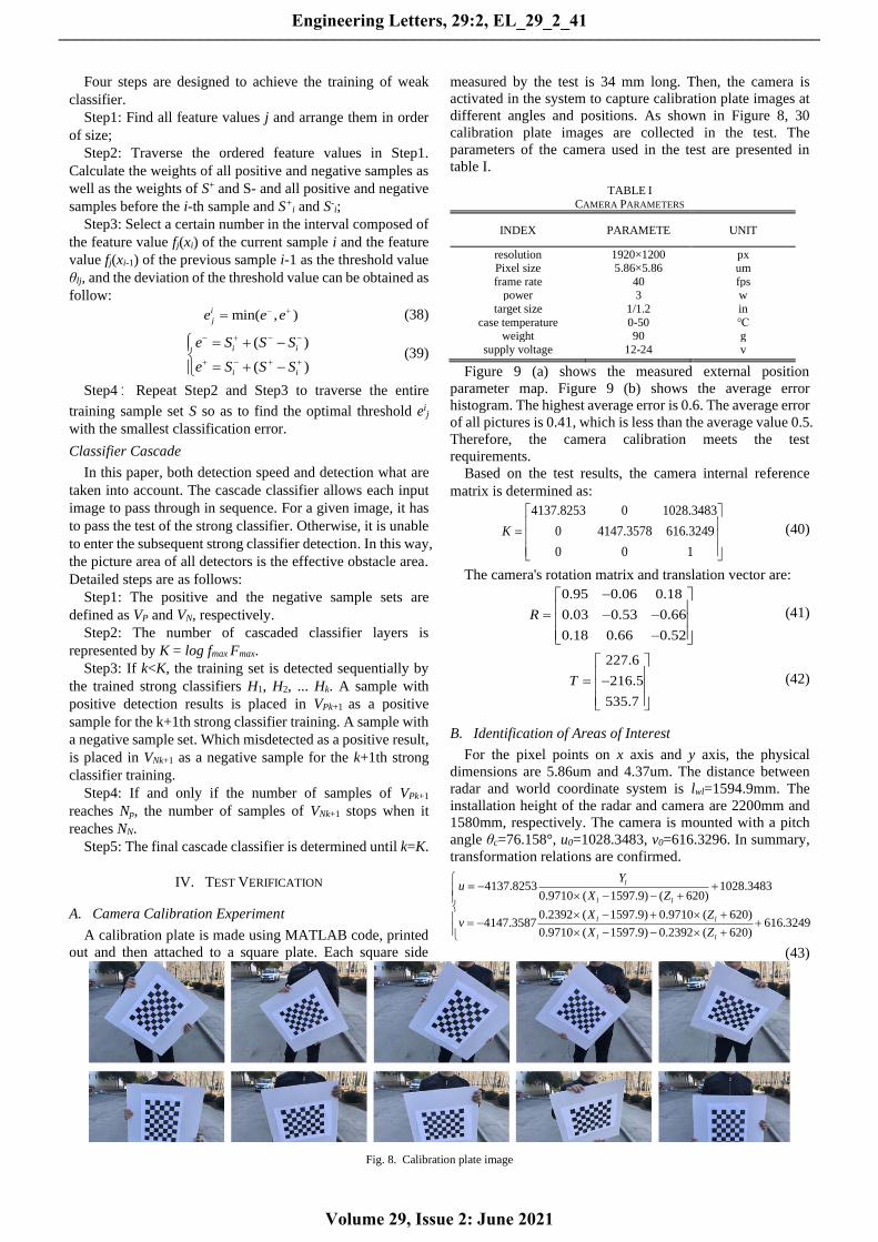
A. Camera Calibration Experiment

A calibration plate is made using MATLAB code, printed

out and then attached to a square plate. Each square side

measured by the test is 34 mm long. Then, the camera is

activated in the system to capture calibration plate images at

different angles and positions. As shown in Figure 8, 30

calibration plate images are collected in the test. The

parameters of the camera used in the test are presented in

table I.

TABLE I

CAMERA PARAMETERS

INDEX PARAMETE UNIT

resolution 1920×1200 px Pixel size 5.86×5.86 um

frame rate 40 fps power 3 w

target size 1/1.2 in

case temperature 0-50 ℃ weight 90 g

supply voltage 12-24 v

Figure 9 (a) shows the measured external position

parameter map. Figure 9 (b) shows the average error

histogram. The highest average error is 0.6. The average error

of all pictures is 0.41, which is less than the average value 0.5.

Therefore, the camera calibration meets the test

requirements.

Based on the test results, the camera internal reference

matrix is determined as:

4137.8253 0 1028.3483

0 4147.3578 616.3249

0 0 1

K

=

(40)

The camera's rotation matrix and translation vector are:

0.95 0.06 0.18

0.03 0.53 0.66

0.18 0.66 0.52

R

−

= − − −

(41)

227.6

216.5

535.7

T

= −

(42)

B. Identification of Areas of Interest

For the pixel points on x axis and y axis, the physical

dimensions are 5.86um and 4.37um. The distance between

radar and world coordinate system is lwl=1594.9mm. The

installation height of the radar and camera are 2200mm and

1580mm, respectively. The camera is mounted with a pitch

angle θc=76.158°, u0=1028.3483, v0=616.3296. In summary,

transformation relations are confirmed.

4137.8253 1028.34830.9710 ( 1597.9) ( 620)

0.2392 ( 1597.9) 0.9710 ( 620)4147.3587 616.3249

0.9710 ( 1597.9) 0.2392 ( 620)

l

l l

l l

l l

Yu

X Z

X Zv

X Z

= − + − − +

− + + = − +

− − +

(43)

Fig. 8. Calibration plate image



______________________________________________________________________________________

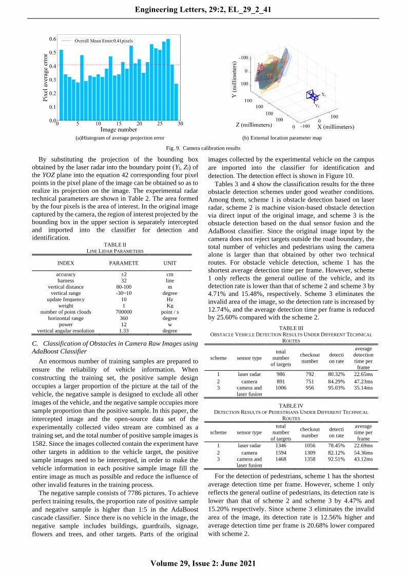
(a)Histogram of average projection error (b) External location parameter map

Fig. 9. Camera calibration results

By substituting the projection of the bounding box

obtained by the laser radar into the boundary point (Yl, Zl) of

the YOZ plane into the equation 42 corresponding four pixel

points in the pixel plane of the image can be obtained so as to

realize its projection on the image. The experimental radar

technical parameters are shown in Table 2. The area formed

by the four pixels is the area of interest. In the original image

captured by the camera, the region of interest projected by the

bounding box in the upper section is separately intercepted

and imported into the classifier for detection and

identification. TABLE II

LINE LIDAR PARAMETERS

INDEX PARAMETE UNIT

accuracy ±2 cm harness 32 line

vertical distance 80-100 m vertical range -30~10 degree

update frequency 10 Hz

weight 1 Kg number of point clouds 700000 point / s

horizontal range 360 degree power 12 w

vertical angular resolution 1.33 degree

C. Classification of Obstacles in Camera Raw Images using

AdaBoost Classifier

An enormous number of training samples are prepared to

ensure the reliability of vehicle information. When

constructing the training set, the positive sample design

occupies a larger proportion of the picture at the tail of the

vehicle, the negative sample is designed to exclude all other

images of the vehicle, and the negative sample occupies more

sample proportion than the positive sample. In this paper, the

intercepted image and the open-source data set of the

experimentally collected video stream are combined as a

training set, and the total number of positive sample images is

1582. Since the images collected contain the experiment have

other targets in addition to the vehicle target, the positive

sample images need to be intercepted, in order to make the

vehicle information in each positive sample image fill the

entire image as much as possible and reduce the influence of

other invalid features in the training process.

The negative sample consists of 7786 pictures. To achieve

perfect training results, the proportion rate of positive sample

and negative sample is higher than 1:5 in the AdaBoost

cascade classifier. Since there is no vehicle in the image, the

negative sample includes buildings, guardrails, signage,

flowers and trees, and other targets. Parts of the original

images collected by the experimental vehicle on the campus

are imported into the classifier for identification and

detection. The detection effect is shown in Figure 10.

Tables 3 and 4 show the classification results for the three

obstacle detection schemes under good weather conditions.

Among them, scheme 1 is obstacle detection based on laser

radar, scheme 2 is machine vision-based obstacle detection

via direct input of the original image, and scheme 3 is the

obstacle detection based on the dual sensor fusion and the

AdaBoost classifier. Since the original image input by the

camera does not reject targets outside the road boundary, the

total number of vehicles and pedestrians using the camera

alone is larger than that obtained by other two technical

routes. For obstacle vehicle detection, scheme 1 has the

shortest average detection time per frame. However, scheme

1 only reflects the general outline of the vehicle, and its

detection rate is lower than that of scheme 2 and scheme 3 by

4.71% and 15.48%, respectively. Scheme 3 eliminates the

invalid area of the image, so the detection rate is increased by

12.74%, and the average detection time per frame is reduced

by 25.60% compared with the scheme 2.

TABLE III OBSTACLE VEHICLE DETECTION RESULTS UNDER DIFFERENT TECHNICAL

ROUTES

scheme sensor type total

number

of targets

checkout

number

detecti

on rate

average

detection

time per frame

1 laser radar 986 792 80.32% 22.65ms

2 camera 891 751 84.29% 47.23ms 3 camera and

laser fusion

1006 956 95.03% 35.14ms

TABLE IV

DETECTION RESULTS OF PEDESTRIANS UNDER DIFFERENT TECHNICAL

ROUTES

scheme sensor type total

number

of targets

checkout number

detection rate

average time per

frame

1 laser radar 1346 1056 78.45% 22.69ms

2 camera 1594 1309 82.12% 54.36ms

3 camera and laser fusion

1468 1358 92.51% 43.12ms

For the detection of pedestrians, scheme 1 has the shortest

average detection time per frame. However, scheme 1 only

reflects the general outline of pedestrians, its detection rate is

lower than that of scheme 2 and scheme 3 by 4.47% and

15.20% respectively. Since scheme 3 eliminates the invalid

area of the image, its detection rate is 12.56% higher and

average detection time per frame is 20.68% lower compared

with scheme 2.



______________________________________________________________________________________

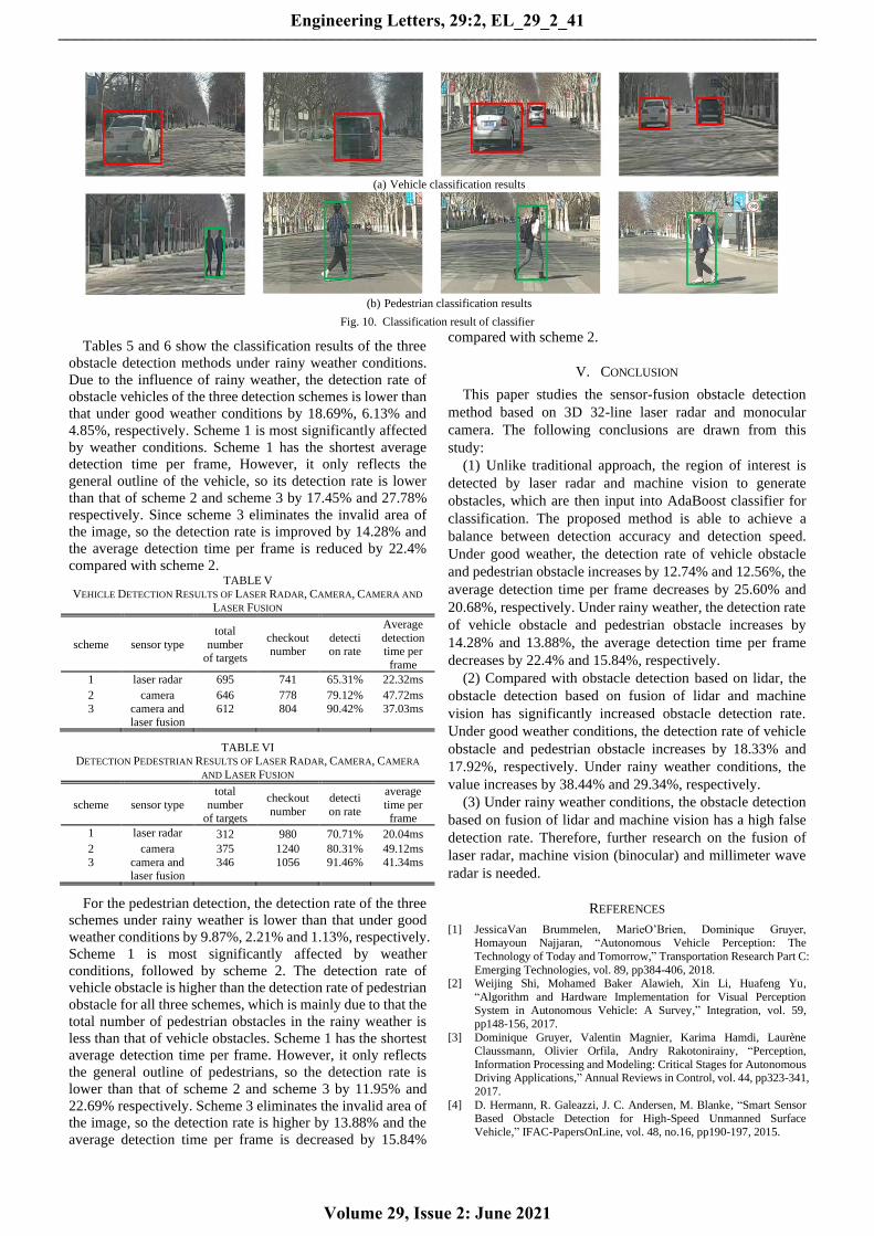
(a) Vehicle classification results

(b) Pedestrian classification results

Fig. 10. Classification result of classifier

Tables 5 and 6 show the classification results of the three

obstacle detection methods under rainy weather conditions.

Due to the influence of rainy weather, the detection rate of

obstacle vehicles of the three detection schemes is lower than

that under good weather conditions by 18.69%, 6.13% and

4.85%, respectively. Scheme 1 is most significantly affected

by weather conditions. Scheme 1 has the shortest average

detection time per frame, However, it only reflects the

general outline of the vehicle, so its detection rate is lower

than that of scheme 2 and scheme 3 by 17.45% and 27.78%

respectively. Since scheme 3 eliminates the invalid area of

the image, so the detection rate is improved by 14.28% and

the average detection time per frame is reduced by 22.4%

compared with scheme 2. TABLE V

VEHICLE DETECTION RESULTS OF LASER RADAR, CAMERA, CAMERA AND

LASER FUSION

scheme sensor type

total

number of targets

checkout number

detection rate

Average

detection time per

frame

1 laser radar 695 741 65.31% 22.32ms

2 camera 646 778 79.12% 47.72ms


612 804 90.42% 37.03ms

TABLE VI DETECTION PEDESTRIAN RESULTS OF LASER RADAR, CAMERA, CAMERA

AND LASER FUSION

scheme sensor type

total

number

of targets

checkout

number

detecti

on rate

average

time per

frame

1 laser radar 312 980 70.71% 20.04ms

2 camera 375 1240 80.31% 49.12ms


346 1056 91.46% 41.34ms

For the pedestrian detection, the detection rate of the three

schemes under rainy weather is lower than that under good

weather conditions by 9.87%, 2.21% and 1.13%, respectively.

Scheme 1 is most significantly affected by weather

conditions, followed by scheme 2. The detection rate of

vehicle obstacle is higher than the detection rate of pedestrian

obstacle for all three schemes, which is mainly due to that the

total number of pedestrian obstacles in the rainy weather is

less than that of vehicle obstacles. Scheme 1 has the shortest

average detection time per frame. However, it only reflects

the general outline of pedestrians, so the detection rate is

lower than that of scheme 2 and scheme 3 by 11.95% and

22.69% respectively. Scheme 3 eliminates the invalid area of

the image, so the detection rate is higher by 13.88% and the

average detection time per frame is decreased by 15.84%

compared with scheme 2.

V. CONCLUSION

This paper studies the sensor-fusion obstacle detection

method based on 3D 32-line laser radar and monocular

camera. The following conclusions are drawn from this

study:

(1) Unlike traditional approach, the region of interest is

detected by laser radar and machine vision to generate

obstacles, which are then input into AdaBoost classifier for

classification. The proposed method is able to achieve a

balance between detection accuracy and detection speed.

Under good weather, the detection rate of vehicle obstacle

and pedestrian obstacle increases by 12.74% and 12.56%, the

average detection time per frame decreases by 25.60% and

20.68%, respectively. Under rainy weather, the detection rate

of vehicle obstacle and pedestrian obstacle increases by

14.28% and 13.88%, the average detection time per frame

decreases by 22.4% and 15.84%, respectively.

(2) Compared with obstacle detection based on lidar, the

obstacle detection based on fusion of lidar and machine

vision has significantly increased obstacle detection rate.

Under good weather conditions, the detection rate of vehicle

obstacle and pedestrian obstacle increases by 18.33% and

17.92%, respectively. Under rainy weather conditions, the

value increases by 38.44% and 29.34%, respectively.

(3) Under rainy weather conditions, the obstacle detection

based on fusion of lidar and machine vision has a high false

detection rate. Therefore, further research on the fusion of

laser radar, machine vision (binocular) and millimeter wave

radar is needed.

REFERENCES

[1] JessicaVan Brummelen, MarieO’Brien, Dominique Gruyer, Homayoun Najjaran, “Autonomous Vehicle Perception: The

Technology of Today and Tomorrow,” Transportation Research Part C:

Emerging Technologies, vol. 89, pp384-406, 2018. [2] Weijing Shi, Mohamed Baker Alawieh, Xin Li, Huafeng Yu,

“Algorithm and Hardware Implementation for Visual Perception System in Autonomous Vehicle: A Survey,” Integration, vol. 59,

pp148-156, 2017.

[3] Dominique Gruyer, Valentin Magnier, Karima Hamdi, Laurène

Claussmann, Olivier Orfila, Andry Rakotonirainy, “Perception,

Information Processing and Modeling: Critical Stages for Autonomous Driving Applications,” Annual Reviews in Control, vol. 44, pp323-341,

2017.

[4] D. Hermann, R. Galeazzi, J. C. Andersen, M. Blanke, “Smart Sensor Based Obstacle Detection for High-Speed Unmanned Surface

Vehicle,” IFAC-PapersOnLine, vol. 48, no.16, pp190-197, 2015.



______________________________________________________________________________________

[5] Jacopo Guanetti, Yeojun Kim, Francesco Borrelli, “Control of Connected and Automated Vehicles: State of the Art and Future

Challenges,” Annual Reviews in Control, vol. 45, pp18-40, 2018.

[6] P. V. Manivannan, Pulidindi Ramakanth, “Vision Based Intelligent

Vehicle Steering Control Using Single Camera for Automated

Highway System,” Procedia Computer Science, vol. 133, pp839-846, 2018.

[7] PEI Xiaofei, LIU Zhaodu, MA Guocheng, YE Yang, “Safe Distance Model and Obstacle Detection Algorithms for A Collision Warning

and Collision Avoidance System,” Journal of Automotive Safety and

Energy, vol. 3, no.1, pp26-33, 2016. [8] Liang Wang, Yihuan Zhang, Jun Wang, “Map-Based Localization

Method for Autonomous Vehicles Using 3D-LIDAR,” IFAC-PapersOnLine, vol. 50, no.1, pp276-281, 2017.

[9] Chen, S., Huang, L., Bai, J., Jiang, H. et al., "Multi-Sensor Information

Fusion Algorithm with Central Level Architecture for Intelligent Vehicle Environmental Perception System," SAE Technical Paper

2016-01-1894, 2016. [10] Guan Xin, Hong Feng, Jia Xin, Zhang Yonghe, Bao Han, “A Research

on the Environmental Perception Method in Intelligent Vehicle

Simulation Based on Layered Information Database,” Automotive Engineering, vol. 37, no.1, pp43-48, 2015.

[11] Wang T, Zheng N, Xin J, et al., “Integrating Millimeter Wave Radar with a Monocular Vision Sensor for On-road Obstacle Detection

Applications,” Sensors, vol. 11, no.9, pp8992-9008, 2011.

[12] M. Bertozzi, A. Broggi, A. Fascioli and S. Nichele, “Stereo vision-based vehicle detection,” Proceedings of the IEEE Intelligent

Vehicles Symposium 2000 (Cat. No.00TH8511), pp39-44, 2000. [13] Zhang Yi, “Stereo-based Research on Obstacles Detection in

Unstructured Environment,” Master's thesis, Beijing Institute of

Technology, Beijing, China, 2015. [14] Mahlisch M, Schweiger R, Ritter W, et al., “Sensorfusion Using

Spatio-Temporal Aligned Video and Lidar for Improved Vehicle Detection,” 2006 IEEE Intelligent Vehicles Symposium, pp424-429,

2006.

[15] Zhang Shuangxi, “Research on Obstacle Detection Technology Based on Radar and Camera of Driverless Smart Vehicles,” Master's thesis,

Chang’an University, Xi’an, China, 2013. [16] Wang Z, Chen B, Wu J, et al., “Real-time Image Tracking with An

Adaptive Complementary Filter,” IAENG International Journal of

Computer Science, vol. 45, no.1, pp97-103, 2018.



______________________________________________________________________________________

Obstacle Detection of Intelligent Vehicle Based on Fusion ...

Documents

Transcript of Obstacle Detection of Intelligent Vehicle Based on Fusion ...