1

Supporting Information. Chauvier, Y., W. Thuiller, P. Brun, S. Lavergne, P. Descombes, D.N. Karger, J. Renaud, N.E. Zimmermann. 2020. Influence of climate, soil, and land cover on plant species distribution in the European Alps. Ecological Monographs.

Appendix S1

Table S1. Complete list of sources of species observations.

Sources Observations count Contribution (%)

AAAAA 110033 1.13432 ACASC 5 0.00005 ACBOG 7 0.00007 ACERC 36 0.00037 ACFA 2654 0.02736 ACFJ 1517 0.01564 ADDHY 13 0.00013 AFASC 6 0.00006 AGIR 311 0.00321 AIPHY 1902 0.01961 ALOBO 30 0.00031 ALPAG 6 0.00006 AMBHH 94 0.00097 ANEMO 6 0.00006 ANSES 68 0.00070 AOOPL 12 0.00012 ASACR 152 0.00157 ASSGV 10345 0.10665 ASTER 10808 0.11142 ATFHA 121809 1.25571 AUBAN 27761 0.28618 AVENI 2048 0.02111 AVIVE 6 0.00006 BARBY 15 0.00015 BARTH 58 0.00060 BBRYS 3 0.00003 BDMZ7 208542 2.14984 BDONF 12694 0.13086 BIODI 17 0.00018 BIOTE 73 0.00075

2

BIOTO 1107 0.01141 BMDZ9 62612 0.64546 BOLIE 2 0.00002 BUGEY 573 0.00591 CAREN 366 0.00377 CAT07 8851 0.09124 CBNA 1929637 19.89241 CBNBR 2 0.00002 CBNMC 120 0.00124 CBNME 1377 0.01420 CBNMED 443991 4.57705 CCEAU 365 0.00376 CEFMB 353 0.00364 CEMAG 13749 0.14174 CENP 2942 0.03033 Cerabo 585 0.00603 CERFF 1 0.00001 CESAM 3 0.00003 CG04 1 0.00001 CG05 93 0.00096 CG38 22 0.00023 CGENE 358 0.00369 CHLAU 6390 0.06587 CINCL 7 0.00007 CLEDA 44 0.00045 CLREJ 114 0.00118 CNR 27 0.00028 CNRS 42 0.00043 CPNS 35095 0.36179 CREN 9826 0.10130 CSOSA 4 0.00004 DDCGI 43 0.00044 DELTH 2401 0.02475 DIRER 2 0.00002 DISEQUALP 30307 0.31243 ECODI 55393 0.57104 ECOMD 5 0.00005 ECOME 9591 0.09887 ECOSP 2100 0.02165 ECOTE 875 0.00902 ECOTP 3 0.00003 EDE 276 0.00285 EDINB 7 0.00007

3

EHB 19947 0.20563 ENGRE 3924 0.04045 EPS 8139 0.08390 ESITP 103 0.00106 EVINE 358 0.00369 FFG 13 0.00013 FLAVI 2019 0.02081 FLOCO 72 0.00074 FLOJU 73 0.00075 FMBDS 8 0.00008 FONPV 9 0.00009 FRAPN 2542 0.02621 FUB 245 0.00253 GBIF 212078 2.18629 GENTI 2119 0.02184 GINGE 86 0.00089 GIRZU 5 0.00005 GLYON 3 0.00003 GMBVS 5 0.00005 HBCAS 13 0.00013 HBGEN 38 0.00039 HCBGE 1 0.00001 HERBG 18 0.00019 HERZO 8 0.00008 IFN 17 0.00018 IMBE 97 0.00100 INERM 1538 0.01586 INFLO 174285 1.79668 InfoFlora 4730449 48.76566 JORDE 202215 2.08461 KarstData 27337 0.28181 LABIO 1897 0.01956 LAVAN 428 0.00441 LECA 158 0.00163 LEPJH 4444 0.04581 LMDPL 229 0.00236 LOPAR 11625 0.11984 LPO 53 0.00055 MENV 252 0.00260 MHNAX 622 0.00641 MHNGR 194 0.00200 MNHN 140 0.00144 NAENV 3892 0.04012

4

NATSC 51 0.00053 NBCO 417 0.00430 NEOT 106 0.00109 NOWBR 37 0.00038 NPLUS 11 0.00011 OCDEE 74 0.00076 ODEPP 5 0.00005 ONCFS 14 0.00014 ONF 10231 0.10547 OXALI 1428 0.01472 PIFH 148 0.00153 PNE 131483 1.35544 PNM 2641 0.02723 PNRC 5 0.00005 PNRLU 2966 0.03058 PNRMB 2649 0.02731 PNRQ 778 0.00802 PNRV 397 0.00409 PNRVE 2 0.00002 PNV 58457 0.60263 RAACF 2854 0.02942 RBNAT 194 0.00200 REBRY 12 0.00012 RECAL 113 0.00116 RESBO 249792 2.57508 RESCB 1709 0.01762 RESYM 12 0.00012 RFRAP 5383 0.05549 RISSO 164 0.00169 RNGL 1 0.00001 RNHCJ 1 0.00001 RNHPV 469 0.00483 RNLAV 490 0.00505 RNNHC 217 0.00224 RNNRV 805 0.00830 RNPLA 1727 0.01780 RNRMV 1 0.00001 RSBO 1 0.00001 RTM 1 0.00001 SA05 13426 0.13841 SAGEE 106 0.00109 SAJA 915 0.00943 SAPN 12 0.00012

5

SAUSS 5 0.00005 SBARD 269 0.00277 SBCOU 1550 0.01598 SBDRO 359 0.00370 SBF 567 0.00585 SBNF 532 0.00548 SCHJO 8491 0.08753 SDETB 918 0.00946 SEGED 20 0.00021 SERAN 965 0.00995 SETIS 1459 0.01504 SFO 65136 0.67148 SHNPM 395 0.00407 SHNSA 163 0.00168 SIABV 856 0.00882 SIERA 23 0.00024 SIGDA 791 0.00815 SIVLO 5 0.00005 SLL 834 0.00860 SLPRO 84 0.00087 SMAVD 105 0.00108 SMBRC 1080 0.01113 SMIGI 37 0.00038 SMVV 4 0.00004 SPCS 1 0.00001 SRTC 36 0.00037 SSLBA 11 0.00011 SYMBH 6436 0.06635 TEREO 223 0.00230 TEVIE 45 0.00046 TINEE 22 0.00023 TUXEN 16 0.00016 TWW 419336 4.32289 UAMSJ 5248 0.05410 UCLBL 64 0.00066 UCOMA 159 0.00164 UIAD 8 0.00008 UMRCA 18 0.00019 UNBES 5404 0.05571 UNCAE 12 0.00012 UNDST 256 0.00264 UNHEI 74 0.00076 UNJOF 47887 0.49366

6

UNPRO 5143 0.05302 UPAR7 1 0.00001 UPAXI 6963 0.07178 VITTE 1 0.00001 WILLNER 61363 0.63258 ZER 24263 0.25012

Text S1. Methodology description of GBIF data extraction and filtering.

To extract GBIF information and merge all datasets, a large list of synonyms of all the plant

species occurring in the European Alps was generated by compiling and web-scrapping information from

different sources: The Catalogue of Life (http://www.catalogueoflife.org/), the Plant List

(http://www.theplantlist.org/) and the CBNA. To generate this list, a search was undertaken across 4490

accepted names referenced in the Flora Alpina Atlas (Aeschimann et al. 2004) to obtain a total of 131.660

synonyms that were used as search inputs on GBIF to retrieve our online observations. Only observations

with a 100% name matching result were kept. GBIF provides a huge amount of georeferenced species

distribution data, but many observations have considerable coordinate uncertainties, duplicated records, or

misleading raster centroids. Therefore, strong spatial and resolution filtering needed to be applied to the

online dataset to make sure that no biased species observations would be used in our models. The filtering

involved mainly: selection based on GBIF’s ‘basis of records’ ("HUMAN_OBSERVATION",

"LITERATURE", "MATERIAL_SAMPLE", "OBSERVATION" and "PRESERVED_SPECIMEN" kept)

and ‘coordinateUncertainties’ (removal when more than 500m), removal of observation duplicates,

removal of observations older than 1980, removal of coordinates with less than three decimals, and

removal of raster centroid datasets (Zizka et al. 2019).

7

Table S2. Summary of species number per elevation belt (Colline, Montane, Sub-alpine, Alpine, and Nival species) and according to three vegetation types (Tree, Herbaceous and Shrub species). 30 species remained unknown due to missing information in Flora Alpina (Aeschimann et al. 2004).

Tree Herbaceous Shrub Unknown Total

Nival 0 99 9 - 108

Alpine 0 272 20 - 292

Sub-Alpine 11 532 58 - 601

Montane 33 854 87 - 974

Colline 40 488 83 - 611

Unknown - - - - 30

Total 84 2245 257 30 2'616

Table S3. Summary of species number per elevation belt (Colline, Montane, Sub-alpine, Alpine, and Nival species) and according to three geological preferences (Calcareous, Siliceous and Mixed species). 30 species remained unknown due to missing information in Flora Alpina (Aeschimann et al. 2004).

Calcareous Siliceous Mixed Unknown Total

Nival 31 53 24 - 108

Alpine 139 80 73 - 292

Sub-Alpine 242 86 273 - 601

Montane 424 99 451 - 974

Colline 260 70 281 - 611

Unknown - - - - 30

Total 1096 388 1102 30 2'616

8

Table S4. Names and descriptions of predictors considered in this study. CHELSA: Climatologies at High resolution for the Earth’s Land Surface Areas, IHME: International Hydrogeological Map of Europe, ESDAC: European Soil Data Centre, ESDD: European Soil Derived Database.

CHELSA: Annual Mean Temperature Climate bio_01 CHELSA: Mean Temperature of Coldest Quarter Climate bio_11 CHELSA: Mean Temperature of Warmest Quarter Climate bio_10 CHELSA: Summer to Winter differences in average daily mean temp. Climate bio_10m11 CHELSA: Min Temperature of Coldest Month Climate bio_06 CHELSA: Max Temperature of Warmest Month Climate bio_05 CHELSA: Temperature Annual Range Climate bio_07 CHELSA: Mean Diurnal Range Climate bio_02 CHELSA: Annual Precipitation Sum Climate bio_12 CHELSA: Precipitation of Coldest Quarter Climate bio_19 CHELSA: Precipitation of Warmest Quarter Climate bio_18 CHELSA: Summer to Winter differences in average daily sum precip. Climate bio_18m19 CHELSA: Precipitation of Driest Month Climate bio_14 CHELSA: Precipitation of Wettest Month Climate bio_13 CHELSA: Precipitation Annual Range Climate bio_13m14 CHELSA: Precipitation Seasonality Climate bio_15 CHELSA: Temperature Seasonality Climate bio_04 CHELSA: Isothermality Climate bio_03 CHELSA: Aridity Climate aridity CHELSA: Frost Frequency Climate frost CHELSA: Snow cover length Climate snow_days CHELSA: Snow cover amount Climate snow_water CHELSA: Growing Season Length Climate GSL_5degrees CHELSA: Growing Season Temp. Climate GST_5degrees CHELSA: Growing degree days Climate GDD_5 CHELSA: Annual Solar radiation Climate srad GLiM - Global lithological map: Calcareous 100m aggregation Soil GLIM_cal_Btype GLiM - Global lithological map: Silicious 100m aggregation Soil GLIM_sil_Btype GLiM - Global lithological map: Mixed 100m aggregation Soil GLIM_mix_Btype IHME - Hydrogeological Map of Europe: Calcareous 100m aggregation Soil IHME_cal_Btype IHME - Hydrogeological Map of Europe: Silicious 100m aggregation Soil IHME_sil_Btype IHME - Hydrogeological Map of Europe: Mixed 100m aggregation Soil IHME_mix_Btype SOILGRIDS: pH in KCL Soil PHIKCL SOILGRIDS: Soil organic carbon density Soil ocdens SOILGRIDS: Absolute depth to bedrock Soil bdticm SOILGRIDS: Clay content Soil clyppt

Name Type Abbreviation

9

SOILGRIDS: Silt content Soil sltppt SOILGRIDS: Sand content Soil sndppt SOILGRIDS: Cation exchange capacity Soil cecsol SOILGRIDS: Available soil water capacity until wilting point Soil wwp ESDAC: topsoil organic content 2004 Soil topsoil_oc ESDAC: ESDD organic carbone content 2013 Soil eu_oc ESDAC: ESDD Depth available to roots 2013 Soil eu_depth_roots ESDAC: ESDD Clay content 2013 Soil eu_clay ESDAC: ESDD Silt content 2013 Soil eu_silt ESDAC: ESDD Sand content 2013 Soil eu_sand ESDAC: ESDD Total available water capacity 2013 Soil eu_tawc ESDAC: Water content at field capacity 3D 2017 Soil eu_fc ESDAC: Saturated hydraulic conductivity 3D 2017 Soil eu_ks ESDAC: ESDD Bulk density 2013 Soil eu_bd ESDAC: ESDD Coarse fragments 2013 Soil eu_gravel CORINE: Built up areas 100m aggregation Land cover C_built CORINE: Agricultural areas 100m aggregation Land cover C_agric CORINE: Forests 100m aggregation Land cover C_forests CORINE: Grasslands 100m aggregation Land cover C_grass CORINE: Open spaces few vegetation 100m aggregation Land cover C_open CORINE: Wetlands 100m aggregation Land cover C_wetlands CORINE: Water 100m aggregation Land cover C_water MODIS - Summer Enhanced Vegetation Index Land cover EVI_season

10

Table S5. Bedrock type classification based on the GLiM soil lithology.

Carbonate sedimentary rocks Calcareous Basic plutonic rocks Calcareous Basic volcanic rocks Calcareous Unconsolidated sediments Mixed Mixed sedimentary rocks Mixed Pyroclastic Mixed Evaporites Mixed Intermediate plutonic rocks Mixed Intermediate volcanic rocks Mixed Siliciclastic sedimentary rocks Siliceous Metamorphic rocks Siliceous Acid plutonic rocks Siliceous Acid volcanic rocks Siliceous

Table S6. Bedrock type classification based on the IHME1500 soil lithology.

Calcareous rocks Calcareous Calcareous rocks and coarse sediments Calcareous Calcareous rocks and fine sediments Calcareous Coarse sediments Mixed Fine sediments Mixed Magmatic rocks Mixed Metamorphic rocks Siliceous Siliciclastic rocks Siliceous Siliciclastic rocks and coarse sediments Siliceous Siliciclastic rocks and fine sediments Siliceous

Soil lithology Bedrock Type

Soil lithology Bedrock Type

11

Table S7. Study’s land cover classification based on CORINE Land Cover level 1.

Artificial surfaces Built up areas Agricultural areas Agricultural areas Forest and semi natural areas Forests Forest and semi natural areas Grasslands Forest and semi natural areas Open spaces with little or no vegetation Wetlands Wetlands Water Water

CORINE Level 1 Land cover classification

12

Table S8. Parallel between land cover classification of the study and CORINE level 2 & 3 classification.

Label - Study Label CORINE Level 2 Label CORINE Level 3Built_up_areas Urban fabric Continuous urban fabricBuilt_up_areas Urban fabric Discontinuous urban fabricBuilt_up_areas Industrial, commercial and transport units Industrial or commercial unitsBuilt_up_areas Industrial, commercial and transport units Road and rail networks and associated landBuilt_up_areas Industrial, commercial and transport units Port areasBuilt_up_areas Industrial, commercial and transport units AirportsBuilt_up_areas Mine, dump and construction sites Mineral extraction sitesBuilt_up_areas Mine, dump and construction sites Dump sitesBuilt_up_areas Mine, dump and construction sites Construction sitesBuilt_up_areas Artificial, non-agricultural vegetated areas Green urban areasBuilt_up_areas Artificial, non-agricultural vegetated areas Sport and leisure facilitiesAgricultural_areas Arable land Non-irrigated arable landAgricultural_areas Arable land Permanently irrigated landAgricultural_areas Arable land Rice fieldsAgricultural_areas Permanent crops VineyardsAgricultural_areas Permanent crops Fruit trees and berry plantationsAgricultural_areas Permanent crops Olive grovesAgricultural_areas Pastures PasturesAgricultural_areas Heterogeneous agricultural areas Annual crops associated with permanent cropsAgricultural_areas Heterogeneous agricultural areas Complex cultivation patternsAgricultural_areas Heterogeneous agricultural areas Land principally occupied by agricultureAgricultural_areas Heterogeneous agricultural areas Agro-forestry areasForests Forests Broad-leaved forestForests Forests Coniferous forestForests Forests Mixed forestGrasslands Scrub and/or herbaceous vegetation associations Natural grasslandsGrasslands Scrub and/or herbaceous vegetation associations Moors and heathlandGrasslands Scrub and/or herbaceous vegetation associations Sclerophyllous vegetationGrasslands Scrub and/or herbaceous vegetation associations Transitional woodland-shrubOpen_spaces_few_vegetation Open spaces with little or no vegetation Beaches, dunes, sandsOpen_spaces_few_vegetation Open spaces with little or no vegetation Bare rocksOpen_spaces_few_vegetation Open spaces with little or no vegetation Sparsely vegetated areasOpen_spaces_few_vegetation Open spaces with little or no vegetation Burnt areasOpen_spaces_few_vegetation Open spaces with little or no vegetation Glaciers and perpetual snowWetlands Wetlands Inland marshesWetlands Wetlands Peat bogsWetlands Wetlands Salt marshesWetlands Wetlands SalinesWetlands Wetlands Intertidal flatsWater Water Water coursesWater Water Water bodiesWater Marine waters Coastal lagoonsWater Marine waters EstuariesWater Marine waters Sea and ocean

13

Figure S1. Pearson correlation tests between climate PCA axes and original climate predictors. Climate has 27 variables and six axes.

Figure S2. Pearson correlation tests between soil PCA axes and original soil predictors. Soil has 25 variables and nine axes.

Figure S3. Pearson correlation tests between land cover PCA axes and original land cover predictors. Land cover has eight variables and six axes.

14

Text S2. Complementary results of PCA predictors’ relationships with original predictors.

PCA axes obtained hold different relationships with our original predictors set. Climate axis

1 (explaining 50.35%) was positively correlated with predictors related to temperature (i.e. bio1,

bio5-6, bio10-11, solar radiations, Growing Season Temperature (GST), Growing Season Length

(GSL), Growing Degree Days (GDD)), and negatively correlated with predictors related to snow

(snow cover length/amount) and precipitations variables (bio12-14, bio18-19, bio13 - bio14, bio18 -

bio19, aridity). Soil axis 1 (explaining 24.49%) was positively correlated with all predictors related to

carbon content, negatively correlated with all predictors related to pH and soil depth, and more

negatively than positively correlated with water content variables. Land cover axis 1 (explaining 24.28%)

was positively correlated with ‘Built-up areas’, ‘Agricultural areas’, ‘Grasslands’, ‘Open spaces with

little or no vegetation’, ‘Wetlands’ and ‘Water’, and negatively correlated with ‘EVI’ and

‘Forests’ (see Fig. S1, S2, S3 for exhaustive correlations between all predictors and axes)

Figure S4. Pearson correlation tests between every environmental principal components and bias covariates considered in our models. Climate had six axes (C1-C6), soil had nine axes (S1-S9) and land cover had six axes (L1-L6). ‘Dist_roads’ stands for ‘Distance to Roads’ and ‘Dist_cities’ stands for ‘Distance to Cities’. Panel (a) shows Pearson correlation tests results, and panel (b) describes whether (TRUE) or not (FALSE) Pearson correlation coefficient |r|> 0.7.

15

Table S9. List of chosen 145 species to model responses along single environmental gradients.

n° Scientific Name Elevation Class

1 Androsace adfinis puberula Alpine 2 Androsace obtusifolia Alpine 3 Antennaria carpatica Alpine 4 Anthyllis vulneraria alpestris Alpine 5 Campanula barbata Alpine 6 Campanula scheuchzeri Alpine 7 Cardamine alpina Alpine 8 Carex lachenalii Alpine 9 Carex sempervirens Alpine

10 Crepis kerneri Alpine 11 Dianthus alpinus Alpine 12 Euphrasia alpina Alpine 13 Galium megalospermum Alpine 14 Galium pseudohelveticum Alpine 15 Gentiana alpina Alpine 16 Leontodon montanus montanus Alpine 17 Lotus alpinus Alpine 18 Luzula alpina Alpine 19 Minuartia recurva Alpine 20 Nardus stricta Alpine 21 Pulsatilla alpina alpina Alpine 22 Ranunculus montanus Alpine 23 Saxifraga paniculata Alpine 24 Silene suecica Alpine 25 Soldanella alpina Alpine 26 Soldanella pusilla Alpine 27 Taraxacum alpinum Alpine 28 Allium neapolitanum Colline 29 Anchusa italica Colline 30 Anthemis gerardiana Colline 31 Asplenium petrarchae Colline 32 Bidens frondosa Colline 33 Carlina corymbosa Colline 34 Castanea sativa Colline 35 Centaurea collina Colline 36 Cistus albidus Colline 37 Coris monspeliensis Colline 38 Corrigiola litoralis Colline

16

39 Cyperus esculentus Colline 40 Erica scoparia Colline 41 Erodium ciconium Colline 42 Fraxinus ornus Colline 43 Fumaria capreolata Colline 44 Helianthus tuberosus Colline 45 Linum trigynum Colline 46 Lythrum hyssopifolia Colline 47 Medicago orbicularis Colline 48 Myosotis discolor Colline 49 Nigella arvensis Colline 50 Olea europaea Colline 51 Philadelphus coronarius Colline 52 Quercus ilex Colline 53 Quercus pubescens Colline 54 Rubia peregrina Colline 55 Ruta graveolens Colline 56 Stratiotes aloides Colline 57 Trifolium angustifolium Colline 58 Typha domingensis Colline 59 Vinca major Colline 60 Acer platanoides Montane 61 Alyssum ligusticum Montane 62 Anemone nemorosa Montane 63 Bellis perennis Montane 64 Campanula bertolae Montane 65 Cardamine pratensis Montane 66 Carex sylvatica Montane 67 Chrysosplenium oppositifolium Montane 68 Cirsium vulgare Montane 69 Cynoglossum germanicum Montane 70 Dianthus carthusianorum capillifrons Montane 71 Digitalis purpurea Montane 72 Eryngium spinalba Montane 73 Euphorbia seguieriana loiseleurii Montane 74 Fagus sylvatica Montane 75 Gagea lutea burnatii Montane 76 Galium mollugo Montane 77 Genista sagittalis delphinensis Montane 78 Geranium macrorrhizum Montane 79 Holcus lanatus Montane 80 Jasione montana Montane 81 Luzula sylvatica Montane 82 Lycopodiella inundata Montane 83 Misopates orontium Montane

17

84 Ononis striata Montane 85 Polygala serpyllifolia Montane 86 Potentilla rupestris Montane 87 Prunus brigantina Montane 88 Viola reichenbachiana Montane 89 Anthyllis vulneraria carpatica Nival 90 Arabis caerulea Nival 91 Artemisia genipi Nival 92 Campanula cenisia Nival 93 Carex curvula curvula Nival 94 Carex parviflora Nival 95 Cerastium latifolium Nival 96 Cerastium uniflorum Nival 97 Draba dubia Nival 98 Draba tomentosa Nival 99 Elyna myosuroides Nival

100 Eritrichium nanum Nival 101 Gentiana bavarica Nival 102 Gentiana orbicularis Nival 103 Gentiana tenella Nival 104 Juncus trifidus Nival 105 Leontodon hispidus Nival 106 Linaria alpina alpina Nival 107 Phyteuma hemisphaericum Nival 108 Potentilla frigida Nival 109 Pritzelago alpina alpina Nival 110 Ranunculus glacialis Nival 111 Salix herbacea Nival 112 Saxifraga biflora biflora Nival 113 Senecio halleri Nival 114 Senecio incanus incanus Nival 115 Silene exscapa Nival 116 Trisetum spicatum Nival 117 Achillea macrophylla SubAlpine 118 Alnus viridis SubAlpine 119 Androsace lactea SubAlpine 120 Carex juncella SubAlpine 121 Centaurea montana SubAlpine 122 Cicerbita alpina SubAlpine 123 Clematis alpina SubAlpine 124 Crepis pyrenaica SubAlpine 125 Cynosurus cristatus SubAlpine 126 Dactylorhiza cruenta SubAlpine 127 Dryopteris villarii SubAlpine 128 Gentiana purpurea SubAlpine

18

129 Geranium rivulare SubAlpine 130 Hedysarum boutignyanum SubAlpine 131 Hugueninia tanacetifolia SubAlpine 132 Juniperus communis hemisphaerica SubAlpine 133 Laserpitium latifolium SubAlpine 134 Linnaea borealis SubAlpine 135 Linum alpinum SubAlpine 136 Picea abies SubAlpine 137 Ranunculus platanifolius SubAlpine 138 Rhododendron hirsutum SubAlpine 139 Sagina glabra SubAlpine 140 Salix alpina SubAlpine 141 Salix helvetica SubAlpine 142 Salix waldsteiniana SubAlpine 143 Saxifraga aspera SubAlpine 144 Thalictrum aquilegiifolium SubAlpine 145 Trollius europaeus SubAlpine

19

Figure S5. Relationships between climate (blue), soil (red), land cover (green) relative influences and 95th percentile of species elevation values in meters. Statistical analyses were done with 2nd order polynomial linear regression. First row represents the unfiltered statistical relationship (all BIFULL) with climate (R2

adj ~ 6.37%, p-value < 0.001), soil (R2adj ~ 3.42%, p-value < 0.001) and land cover (R2

adj ~ 3.76%, p-value < 0.001). Second row represents the filtered statistical relationship (BIFULL > 0.4) with climate (R2

adj ~ 5.24%, p-value < 0.001), soil (R2adj ~ 2.78%, p-value < 0.01) and land cover (R2

adj ~ 3.38%, p-value < 0.001); each one respectively represented in Fig. 4b. The filtered version was applied to correct for non-realistic relative values of 0 and 100%. Colored shades show 95% prediction interval. Number of species for filtered and unfiltered results remained the same. See Table S10 for more information on models comparison, results and strength.

20

Figure S6. Relationships between climate (blue), soil (red), land cover (green) absolute influences and 95th percentile of species elevation values in meters. Statistical analyses were done with 2nd order polynomial linear regression. First row represents the unfiltered statistical relationship (all BIFULL) with climate (R2

adj ~ 11.10%, p-value < 0.001), soil (R2adj ~ 6.70%, p-value < 0.001) and land cover (R2

adj ~ 1.26%, p-value < 0.001). Second row represents the filtered statistical relationship (BIFULL > 0.4) with climate (R2

adj ~ 18.66%, p-value < 0.001), soil (R2adj ~ 11.85%, p-value < 0.001) and land cover (R2

adj ~ 5.27%, p-value < 0.001). Colored shades show 95% prediction interval. Number of species for filtered and unfiltered results remained the same. See Table S10 for more information on models comparison, results and strength.

21

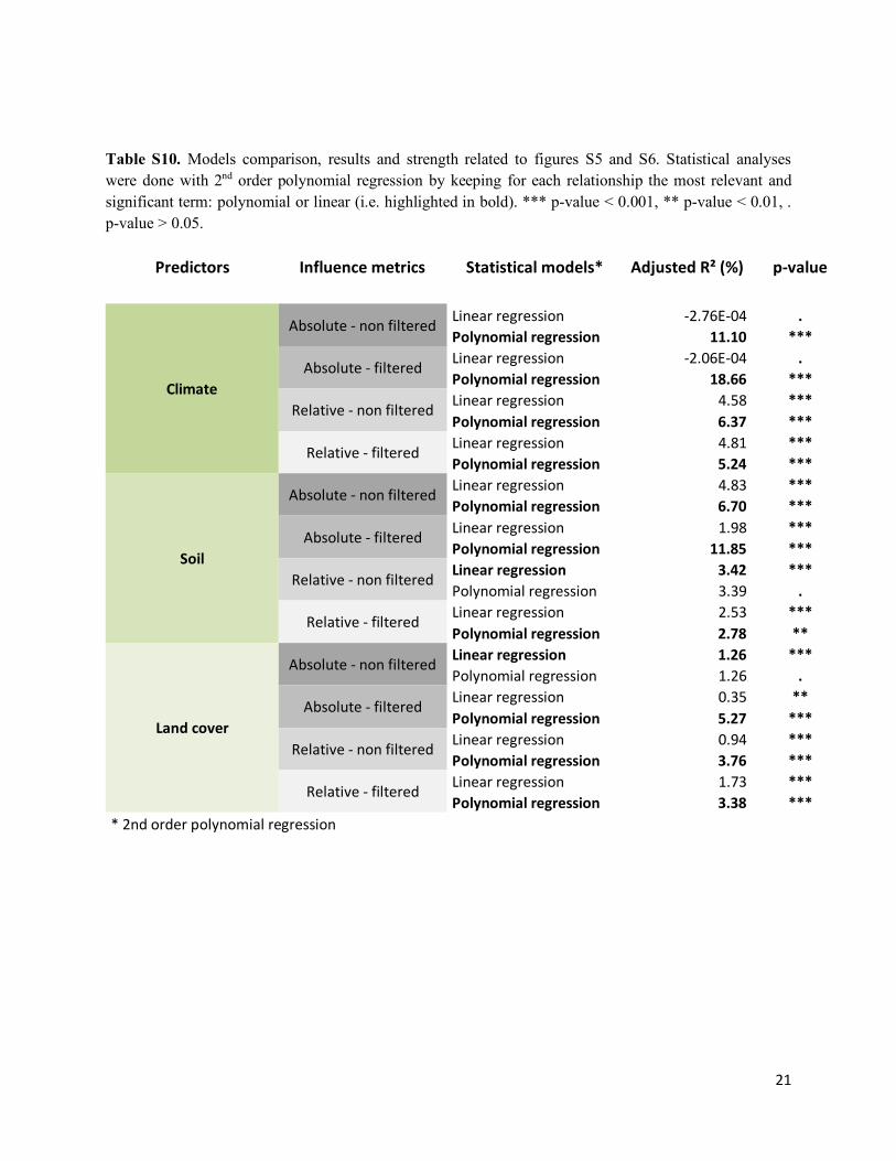
Predictors Influence metrics Statistical models* Adjusted R² (%) p-value

Climate

Absolute - non filtered Linear regression -2.76E-04 . Polynomial regression 11.10 ***

Absolute - filtered Linear regression -2.06E-04 . Polynomial regression 18.66 ***

Relative - non filtered Linear regression 4.58 *** Polynomial regression 6.37 ***

Relative - filtered Linear regression 4.81 *** Polynomial regression 5.24 ***

Soil

Absolute - non filtered Linear regression 4.83 *** Polynomial regression 6.70 ***

Absolute - filtered Linear regression 1.98 *** Polynomial regression 11.85 ***

Relative - non filtered Linear regression 3.42 *** Polynomial regression 3.39 .

Relative - filtered Linear regression 2.53 *** Polynomial regression 2.78 **

Land cover

Absolute - non filtered Linear regression 1.26 *** Polynomial regression 1.26 .

Absolute - filtered Linear regression 0.35 ** Polynomial regression 5.27 ***

Relative - non filtered Linear regression 0.94 *** Polynomial regression 3.76 ***

Relative - filtered Linear regression 1.73 *** Polynomial regression 3.38 ***

* 2nd order polynomial regression

Table S10. Models comparison, results and strength related to figures S5 and S6. Statistical analyses were done with 2nd order polynomial regression by keeping for each relationship the most relevant and significant term: polynomial or linear (i.e. highlighted in bold). *** p-value < 0.001, ** p-value < 0.01, . p-value > 0.05.

22

Figure S7. Mean distributions of BIFULL along elevation classes for the 2’616 species of the study. Colline species: Col.; Montane species: Mont.; S-Alp: Sub-alpine species; Alpine species: Alp.; Nival species: Niv.

23

Figure S8. Extension of Fig.4. Relationships between relative climate (blue), soil (red), and land cover (green) effects on prediction accuracy and species elevation in meters, for tree, shrub and herbaceous species. The influence is represented (a) per elevation belt and (b) per species plotted at their 95th elevation percentile. *: p-value<0.05, **: p-value<0.01, ***: p-value<0.001; p-values in black describe significance of second order polynomial linear relationships, whereas if orange, only the first order polynomial linear relationship was to be found significant.

24

Figure S9. Extension of Fig.4. Relationships between relative climate (blue), soil (red), and land cover (green) effects on prediction accuracy and species elevation in meters, for calcareous, siliceous and mixed species. The influence is represented (a) per elevation belt and (b) per species plotted at their 95th elevation percentile. *: p-value<0.05, **: p-value<0.01, ***: p-value<0.001; p-values in black describe significance of second order polynomial linear relationships, whereas if orange, only the first order polynomial linear relationship was found significant.

25

Figure S10. Map of the average relative influence of climate (C), soil (S) and land cover (L) of all 2’616 plant species distributions across the European Alps. The relative influences of climate, soil and land cover were stretched by scaling each of the three RGB color layers and mapped as RGB composite. Pure colors of blue stand for dominant effects of climate identified across pixels, red of soil and green of land cover. Mixed colors express join effects of two or three drivers.

26

Figure S11. Climate variability (six PCA axes) in function of elevation in meters. For each PCA predictor, 50’000 points were randomly sampled without replacements, and plotted against elevation EU-DEM values at 1km resolution. Variability was calculated each 400m steps from minimum elevation values to maximum. Grey lines show median, upper orange line 95th percentile and lower orange line 5th percentile.

27

Figure S12. Soil variability (nine PCA axes) in function of elevation in meters. For each PCA predictor, 50’000 points were randomly sampled without replacements, and plotted against elevation EU-DEM values at 1km resolution. Variability was calculated each 400m steps from minimum elevation values to maximum. Grey lines show median, upper blue line 95th percentile and lower blue line 5th percentile.

28

Figure S13. RGB composite raster of soil PCA one, two and three. The three soil PCA grids were stretched by scaling each of the three RGB color layers and mapped as RGB composite. Pure colors of blue stand for dominant soil PCA 1, red of soil PCA 2, and green of soil PCA 3. Mixed colors express join effects of two or three soil PCA.

29

Figure S14. CORINE land cover classification in the European Alps. Classification was made according to CORINE land cover 2012 at 100m resolution and the study’s land cover levels. Panel (a) shows spatially information found in (b). Panel (b) represents for each elevation band the dominant land cover (‘Major’). Panel (c) describes proportions of land cover classes in percentage distributed along elevation bands. Values between bands were interpolated with a spline function for better visualization. Panel (d) shows summary of proportion (%) values for each bands. Values in red are < 1.0% and in blue > 1.0%. ‘Meaningful classes’ described number of classes for each elevation band with proportions > 1.0%. ‘L’: Lowland, ‘C’: Colline, ‘M’: Montane, ‘SA’: SubAlpine, ‘A’: Alpine, ‘SN’: SubNival, ‘N’: Nival.

30

Literature cited

Aeschimann, D. et al. 2004. Flora alpina: ein Atlas sämtlicher 4500 Gefässpflanzen der Alpen.

Zizka, A. et al. 2019. CoordinateCleaner: standardized cleaning of occurrence records from biological collection databases. Methods in Ecology and Evolution 10:744–751.