Observation of High-Energy Astrophysical Neutrinos in Three Years of IceCube Data

M. G. Aartsen,2 M. Ackermann,45 J. Adams,15 J. A. Aguilar,23 M. Ahlers,28 M. Ahrens,36 D. Altmann,22

T. Anderson,42 C. Arguelles,28 T. C. Arlen,42 J. Auffenberg,1 X. Bai,34 S. W. Barwick,25 V. Baum,29

J. J. Beatty,17, 18 J. Becker Tjus,10 K.-H. Becker,44 S. BenZvi,28 P. Berghaus,45 D. Berley,16 E. Bernardini,45

A. Bernhard,31 D. Z. Besson,26 G. Binder,8, 7 D. Bindig,44 M. Bissok,1 E. Blaufuss,16 J. Blumenthal,1

D. J. Boersma,43 C. Bohm,36 D. Bose,38 S. Boser,11 O. Botner,43 L. Brayeur,13 H.-P. Bretz,45 A. M. Brown,15

J. Casey,5 M. Casier,13 D. Chirkin,28 A. Christov,23 B. Christy,16 K. Clark,39 L. Classen,22 F. Clevermann,20

S. Coenders,31 D. F. Cowen,42, 41 A. H. Cruz Silva,45 M. Danninger,36 J. Daughhetee,5 J. C. Davis,17 M. Day,28

J. P. A. M. de Andre,42 C. De Clercq,13 S. De Ridder,24 P. Desiati,28 K. D. de Vries,13 M. de With,9 T. DeYoung,42

J. C. Dıaz-Velez,28 M. Dunkman,42 R. Eagan,42 B. Eberhardt,29 B. Eichmann,10 J. Eisch,28 S. Euler,43

P. A. Evenson,32 O. Fadiran,28 A. R. Fazely,6 A. Fedynitch,10 J. Feintzeig,28, ∗ J. Felde,16 T. Feusels,24

K. Filimonov,7 C. Finley,36 T. Fischer-Wasels,44 S. Flis,36 A. Franckowiak,11 K. Frantzen,20 T. Fuchs,20

T. K. Gaisser,32 J. Gallagher,27 L. Gerhardt,8, 7 D. Gier,1 L. Gladstone,28 T. Glusenkamp,45 A. Goldschmidt,8

G. Golup,13 J. G. Gonzalez,32 J. A. Goodman,16 D. Gora,45 D. T. Grandmont,21 D. Grant,21 P. Gretskov,1

J. C. Groh,42 A. Groß,31 C. Ha,8, 7 C. Haack,1 A. Haj Ismail,24 P. Hallen,1 A. Hallgren,43 F. Halzen,28 K. Hanson,12

D. Hebecker,11 D. Heereman,12 D. Heinen,1 K. Helbing,44 R. Hellauer,16 D. Hellwig,1 S. Hickford,15 G. C. Hill,2

K. D. Hoffman,16 R. Hoffmann,44 A. Homeier,11 K. Hoshina,28, † F. Huang,42 W. Huelsnitz,16 P. O. Hulth,36

K. Hultqvist,36 S. Hussain,32 A. Ishihara,14 E. Jacobi,45 J. Jacobsen,28 K. Jagielski,1 G. S. Japaridze,4 K. Jero,28

O. Jlelati,24 M. Jurkovic,31 B. Kaminsky,45 A. Kappes,22 T. Karg,45 A. Karle,28 M. Kauer,28 J. L. Kelley,28

A. Kheirandish,28 J. Kiryluk,37 J. Klas,44 S. R. Klein,8, 7 J.-H. Kohne,20 G. Kohnen,30 H. Kolanoski,9 A. Koob,1

L. Kopke,29 C. Kopper,28, ∗ S. Kopper,44 D. J. Koskinen,19 M. Kowalski,11 A. Kriesten,1 K. Krings,1 G. Kroll,29

J. Kunnen,13 N. Kurahashi,28 T. Kuwabara,32 M. Labare,24 D. T. Larsen,28 M. J. Larson,19 M. Lesiak-Bzdak,37

M. Leuermann,1 J. Leute,31 J. Lunemann,29 O. Macıas,15 J. Madsen,35 G. Maggi,13 R. Maruyama,28 K. Mase,14

H. S. Matis,8 F. McNally,28 K. Meagher,16 A. Meli,24 T. Meures,12 S. Miarecki,8, 7 E. Middell,45 E. Middlemas,28

N. Milke,20 J. Miller,13 L. Mohrmann,45 T. Montaruli,23 R. Morse,28 R. Nahnhauer,45 U. Naumann,44

H. Niederhausen,37 S. C. Nowicki,21 D. R. Nygren,8 A. Obertacke,44 S. Odrowski,21 A. Olivas,16 A. Omairat,44

A. O’Murchadha,12 T. Palczewski,40 L. Paul,1 O. Penek,1 J. A. Pepper,40 C. Perez de los Heros,43 C. Pfendner,17

D. Pieloth,20 E. Pinat,12 J. Posselt,44 P. B. Price,7 G. T. Przybylski,8 J. Putz,1 M. Quinnan,42 L. Radel,1

M. Rameez,23 K. Rawlins,3 P. Redl,16 I. Rees,28 R. Reimann,1 E. Resconi,31 W. Rhode,20 M. Richman,16

B. Riedel,28 S. Robertson,2 J. P. Rodrigues,28 M. Rongen,1 C. Rott,38 T. Ruhe,20 B. Ruzybayev,32 D. Ryckbosch,24

S. M. Saba,10 H.-G. Sander,29 M. Santander,28 S. Sarkar,19, 33 K. Schatto,29 F. Scheriau,20 T. Schmidt,16

M. Schmitz,20 S. Schoenen,1 S. Schoneberg,10 A. Schonwald,45 A. Schukraft,1 L. Schulte,11 O. Schulz,31 D. Seckel,32

Y. Sestayo,31 S. Seunarine,35 R. Shanidze,45 C. Sheremata,21 M. W. E. Smith,42 D. Soldin,44 G. M. Spiczak,35

C. Spiering,45 M. Stamatikos,17, ‡ T. Stanev,32 N. A. Stanisha,42 A. Stasik,11 T. Stezelberger,8 R. G. Stokstad,8

A. Stoßl,45 E. A. Strahler,13 R. Strom,43 N. L. Strotjohann,11 G. W. Sullivan,16 H. Taavola,43 I. Taboada,5

A. Tamburro,32 A. Tepe,44 S. Ter-Antonyan,6 A. Terliuk,45 G. Tesic,42 S. Tilav,32 P. A. Toale,40 M. N. Tobin,28

D. Tosi,28 M. Tselengidou,22 E. Unger,10 M. Usner,11 S. Vallecorsa,23 N. van Eijndhoven,13 J. Vandenbroucke,28

J. van Santen,28 M. Vehring,1 M. Voge,11 M. Vraeghe,24 C. Walck,36 M. Wallraff,1 Ch. Weaver,28

M. Wellons,28 C. Wendt,28 S. Westerhoff,28 B. J. Whelan,2 N. Whitehorn,28, 7, ∗ C. Wichary,1 K. Wiebe,29

C. H. Wiebusch,1 D. R. Williams,40 H. Wissing,16 M. Wolf,36 T. R. Wood,21 K. Woschnagg,7 D. L. Xu,40

X. W. Xu,6 J. P. Yanez,45 G. Yodh,25 S. Yoshida,14 P. Zarzhitsky,40 J. Ziemann,20 S. Zierke,1 and M. Zoll36

(IceCube Collaboration)1III. Physikalisches Institut, RWTH Aachen University, D-52056 Aachen, Germany

2School of Chemistry & Physics, University of Adelaide, Adelaide SA, 5005 Australia3Dept. of Physics and Astronomy, University of Alaska Anchorage,

3211 Providence Dr., Anchorage, AK 99508, USA4CTSPS, Clark-Atlanta University, Atlanta, GA 30314, USA5School of Physics and Center for Relativistic Astrophysics,Georgia Institute of Technology, Atlanta, GA 30332, USA

6Dept. of Physics, Southern University, Baton Rouge, LA 70813, USA7Dept. of Physics, University of California, Berkeley, CA 94720, USA8Lawrence Berkeley National Laboratory, Berkeley, CA 94720, USA

arX

iv:1

405.

5303

v2 [

astr

o-ph

.HE

] 2

Jul

201

4

2

9Institut fur Physik, Humboldt-Universitat zu Berlin, D-12489 Berlin, Germany10Fakultat fur Physik & Astronomie, Ruhr-Universitat Bochum, D-44780 Bochum, Germany

11Physikalisches Institut, Universitat Bonn, Nussallee 12, D-53115 Bonn, Germany12Universite Libre de Bruxelles, Science Faculty CP230, B-1050 Brussels, Belgium

13Vrije Universiteit Brussel, Dienst ELEM, B-1050 Brussels, Belgium14Dept. of Physics, Chiba University, Chiba 263-8522, Japan

15Dept. of Physics and Astronomy, University of Canterbury, Private Bag 4800, Christchurch, New Zealand16Dept. of Physics, University of Maryland, College Park, MD 20742, USA17Dept. of Physics and Center for Cosmology and Astro-Particle Physics,

Ohio State University, Columbus, OH 43210, USA18Dept. of Astronomy, Ohio State University, Columbus, OH 43210, USA

19Niels Bohr Institute, University of Copenhagen, DK-2100 Copenhagen, Denmark20Dept. of Physics, TU Dortmund University, D-44221 Dortmund, Germany

21Dept. of Physics, University of Alberta, Edmonton, Alberta, Canada T6G 2E122Erlangen Centre for Astroparticle Physics, Friedrich-Alexander-Universitat Erlangen-Nurnberg, D-91058 Erlangen, Germany

23Departement de physique nucleaire et corpusculaire,Universite de Geneve, CH-1211 Geneve, Switzerland

24Dept. of Physics and Astronomy, University of Gent, B-9000 Gent, Belgium25Dept. of Physics and Astronomy, University of California, Irvine, CA 92697, USA26Dept. of Physics and Astronomy, University of Kansas, Lawrence, KS 66045, USA

27Dept. of Astronomy, University of Wisconsin, Madison, WI 53706, USA28Dept. of Physics and Wisconsin IceCube Particle Astrophysics Center,

University of Wisconsin, Madison, WI 53706, USA29Institute of Physics, University of Mainz, Staudinger Weg 7, D-55099 Mainz, Germany

30Universite de Mons, 7000 Mons, Belgium31T.U. Munich, D-85748 Garching, Germany

32Bartol Research Institute and Dept. of Physics and Astronomy,University of Delaware, Newark, DE 19716, USA

33Dept. of Physics, University of Oxford, 1 Keble Road, Oxford OX1 3NP, UK34Dept. of Physics, South Dakota School of Mines and Technology, Rapid City, SD 57701, USA

35Dept. of Physics, University of Wisconsin, River Falls, WI 54022, USA36Oskar Klein Centre and Dept. of Physics, Stockholm University, SE-10691 Stockholm, Sweden37Dept. of Physics and Astronomy, Stony Brook University, Stony Brook, NY 11794-3800, USA

38Dept. of Physics, Sungkyunkwan University, Suwon 440-746, Korea39Dept. of Physics, University of Toronto, Toronto, Ontario, Canada, M5S 1A7

40Dept. of Physics and Astronomy, University of Alabama, Tuscaloosa, AL 35487, USA41Dept. of Astronomy and Astrophysics, Pennsylvania State University, University Park, PA 16802, USA

42Dept. of Physics, Pennsylvania State University, University Park, PA 16802, USA43Dept. of Physics and Astronomy, Uppsala University, Box 516, S-75120 Uppsala, Sweden

44Dept. of Physics, University of Wuppertal, D-42119 Wuppertal, Germany45DESY, D-15735 Zeuthen, Germany

A search for high-energy neutrinos interacting within the IceCube detector between 2010 and2012 provided the first evidence for a high-energy neutrino flux of extraterrestrial origin. Resultsfrom an analysis using the same methods with a third year (2012-2013) of data from the completeIceCube detector are consistent with the previously reported astrophysical flux in the 100 TeV - PeVrange at the level of 10−8 GeV cm−2 s−1 sr−1 per flavor and reject a purely atmospheric explanationfor the combined 3-year data at 5.7σ. The data are consistent with expectations for equal fluxesof all three neutrino flavors and with isotropic arrival directions, suggesting either numerous orspatially extended sources. The three-year data set, with a livetime of 988 days, contains a total of37 neutrino candidate events with deposited energies ranging from 30 to 2000 TeV. The 2000 TeVevent is the highest-energy neutrino interaction ever observed.

High energy neutrinos are expected to be producedin astrophysical objects by the decays of charged pionsmade in cosmic ray interactions with radiation or gas [1–4]. As these pions decay, they produce neutrinos withtypical energies of 5% those of the cosmic ray nucleons[5, 6]. These neutrinos can travel long distances undis-turbed by either the absorption experienced by high-energy photons or the magnetic deflection experienced bycharged particles, making them a unique tracer of cosmic

ray acceleration.

Observations since 2008 using the Antarctic gigatonIceCube detector [7] while it was under construction pro-vided several indications of such neutrinos in a variety ofchannels [8–10]. Two years of data from the full detec-tor, from May 2010 - May 2012, then provided the firststrong evidence for the detection of these astrophysicalneutrinos [11] using an all-flavor all-direction sample ofneutrinos interacting within the detector volume. This

3

analysis focused on neutrinos above 100 TeV, at whichthe expected atmospheric neutrino background falls tothe level of one event per year, allowing any harder as-trophysical flux to be seen clearly. Here, following thesame techniques, we add a third year of data support-ing this result and begin to probe the properties of theobserved astrophysical neutrino flux.

Neutrinos are detected in IceCube by observing theCherenkov light produced in ice by charged particles cre-ated when neutrinos interact. These particles generallytravel distances too small to be resolved individually andthe particle shower is observed only in aggregate. In νµcharged-current (CC) interactions, however, as well asa minority of ντ CC, a high-energy muon is producedthat leaves a visible track (unless produced on the detec-tor boundary heading outward). Although deposited en-ergy resolution is similar for all events, angular resolutionfor events containing visible muon tracks is much better(. 1◦, 50% CL) than for those that do not (∼ 15◦, 50%CL) [12]. For equal neutrino fluxes of all flavors (1:1:1),νµ CC events make up only 20% of interactions [13].

Backgrounds to astrophysical neutrino detection ariseentirely from cosmic ray air showers. Muons produced byπ and K decays above IceCube enter the detector at 2.8kHz. Neutrinos produced in the same interactions [14–17]enter IceCube from above and below, and are seen at amuch lower rate due to the low neutrino interaction cross-section. Because π and K mesons decay overwhelminglyto muons rather than electrons, these neutrinos are pre-dominantly νµ and usually have track-type topologies inthe detector [13]. As the parent meson’s energy rises, itslifetime increases, making it increasingly likely to interactbefore decaying. Both the atmospheric muon and neu-trino fluxes thus become suppressed at high energy, witha spectrum one power steeper than the primary cosmicrays that produced them [18]. At energies above ∼ 100TeV, an analogous flux of muons and neutrinos from thedecay of charmed mesons is expected to dominate, as theshorter lifetime of these particles allows this flux to avoidsuppression from interaction before decay [19–25]. Thisflux has not yet been observed, however, and both itsoverall rate and cross-over energy with the π/K flux areat present poorly constrained [26]. As before [11], we es-timate all atmospheric neutrino background rates usingmeasurements of the northern-hemisphere νµ spectrum[9].

Event selection identifies neutrino interactions in Ice-Cube by rejecting those events with Cherenkov-radiatingparticles, principally cosmic ray muons, entering fromoutside the detector. As before, we used a simple anti-coincidence muon veto in the outer layers of the detector[11], requiring that fewer than 3 of the first 250 detectedphotoelectrons (PE) be on the detector boundary. To en-sure sufficient numbers of photons to reliably trigger thisveto, we additionally required at least 6000 PE overall,corresponding to deposited energies of approximately 30

-80

-60

-40

-20

0

20

40

60

80

102

103

De

clin

atio

n (

de

gre

es)

Deposited EM-Equivalent Energy in Detector (TeV)

ShowersTracks

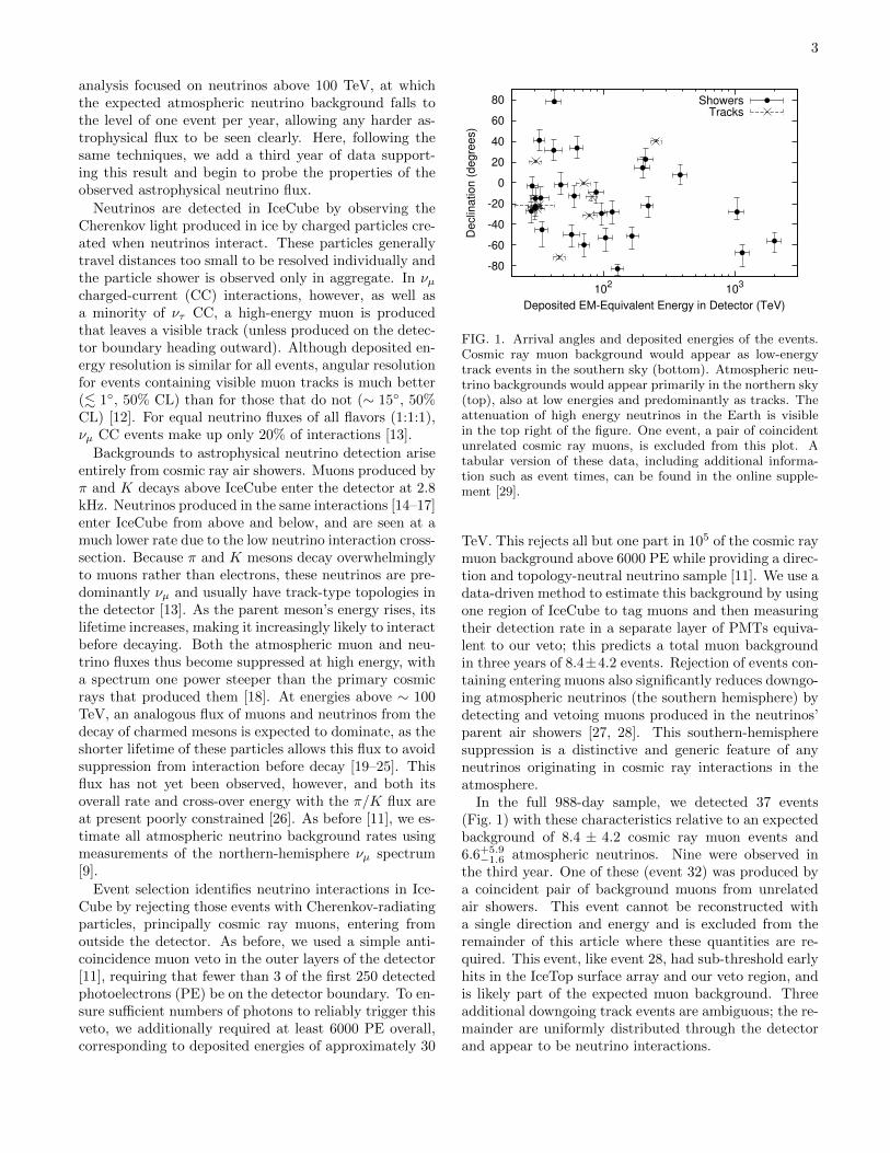
FIG. 1. Arrival angles and deposited energies of the events.Cosmic ray muon background would appear as low-energytrack events in the southern sky (bottom). Atmospheric neu-trino backgrounds would appear primarily in the northern sky(top), also at low energies and predominantly as tracks. Theattenuation of high energy neutrinos in the Earth is visiblein the top right of the figure. One event, a pair of coincidentunrelated cosmic ray muons, is excluded from this plot. Atabular version of these data, including additional informa-tion such as event times, can be found in the online supple-ment [29].

TeV. This rejects all but one part in 105 of the cosmic raymuon background above 6000 PE while providing a direc-tion and topology-neutral neutrino sample [11]. We use adata-driven method to estimate this background by usingone region of IceCube to tag muons and then measuringtheir detection rate in a separate layer of PMTs equiva-lent to our veto; this predicts a total muon backgroundin three years of 8.4±4.2 events. Rejection of events con-taining entering muons also significantly reduces downgo-ing atmospheric neutrinos (the southern hemisphere) bydetecting and vetoing muons produced in the neutrinos’parent air showers [27, 28]. This southern-hemispheresuppression is a distinctive and generic feature of anyneutrinos originating in cosmic ray interactions in theatmosphere.

In the full 988-day sample, we detected 37 events(Fig. 1) with these characteristics relative to an expectedbackground of 8.4 ± 4.2 cosmic ray muon events and6.6+5.9−1.6 atmospheric neutrinos. Nine were observed in

the third year. One of these (event 32) was produced bya coincident pair of background muons from unrelatedair showers. This event cannot be reconstructed witha single direction and energy and is excluded from theremainder of this article where these quantities are re-quired. This event, like event 28, had sub-threshold earlyhits in the IceTop surface array and our veto region, andis likely part of the expected muon background. Threeadditional downgoing track events are ambiguous; the re-mainder are uniformly distributed through the detectorand appear to be neutrino interactions.

4

10-1

100

101

102Events

per

988 D

ays

102 103 104

Deposited EM-Equivalent Energy in Detector (TeV)

Background Atmospheric Muon Flux

Bkg. Atmospheric Neutrinos (π/K)

Background Uncertainties

Atmospheric Neutrinos (90% CL Charm Limit)

Bkg.+Signal Best-Fit Astrophysical (best-fit slope E−2.3 )

Bkg.+Signal Best-Fit Astrophysical (fixed slope E−2 )

Data

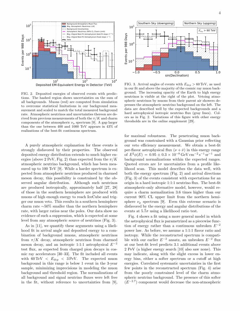
FIG. 2. Deposited energies of observed events with predic-tions. The hashed region shows uncertainties on the sum ofall backgrounds. Muons (red) are computed from simulationto overcome statistical limitations in our background mea-surement and scaled to match the total measured backgroundrate. Atmospheric neutrinos and uncertainties thereon are de-rived from previous measurements of both the π/K and charmcomponents of the atmospheric νµ spectrum [9]. A gap largerthan the one between 400 and 1000 TeV appears in 43% ofrealizations of the best-fit continuous spectrum.

A purely atmospheric explanation for these events isstrongly disfavored by their properties. The observeddeposited energy distribution extends to much higher en-ergies (above 2 PeV, Fig. 2) than expected from the π/Katmospheric neutrino background, which has been mea-sured up to 100 TeV [9]. While a harder spectrum is ex-pected from atmospheric neutrinos produced in charmedmeson decay, this possibility is constrained by the ob-served angular distribution. Although such neutrinosare produced isotropically, approximately half [27, 28]of those in the southern hemisphere are produced withmuons of high enough energy to reach IceCube and trig-ger our muon veto. This results in a southern hemispherecharm rate ∼50% smaller than the northern hemisphererate, with larger ratios near the poles. Our data show noevidence of such a suppression, which is expected at somelevel from any atmospheric source of neutrinos (Fig. 3).

As in [11], we quantify these arguments using a likeli-hood fit in arrival angle and deposited energy to a com-bination of background muons, atmospheric neutrinosfrom π/K decay, atmospheric neutrinos from charmedmeson decay, and an isotropic 1:1:1 astrophysical E−2

test flux, as expected from charged pion decays in cos-mic ray accelerators [30–33]. The fit included all eventswith 60 TeV < Edep < 3 PeV. The expected muonbackground in this range is below 1 event in the 3-yearsample, minimizing imprecisions in modeling the muonbackground and threshold region. The normalizations ofall background and signal neutrino fluxes were left freein the fit, without reference to uncertainties from [9],

10-1

100

101

Events

per

988 D

ays

1.0 0.5 0.0 0.5 1.0sin(Declination)

Northern Sky (upgoing)Southern Sky (downgoing)

Edep > 60 TeV

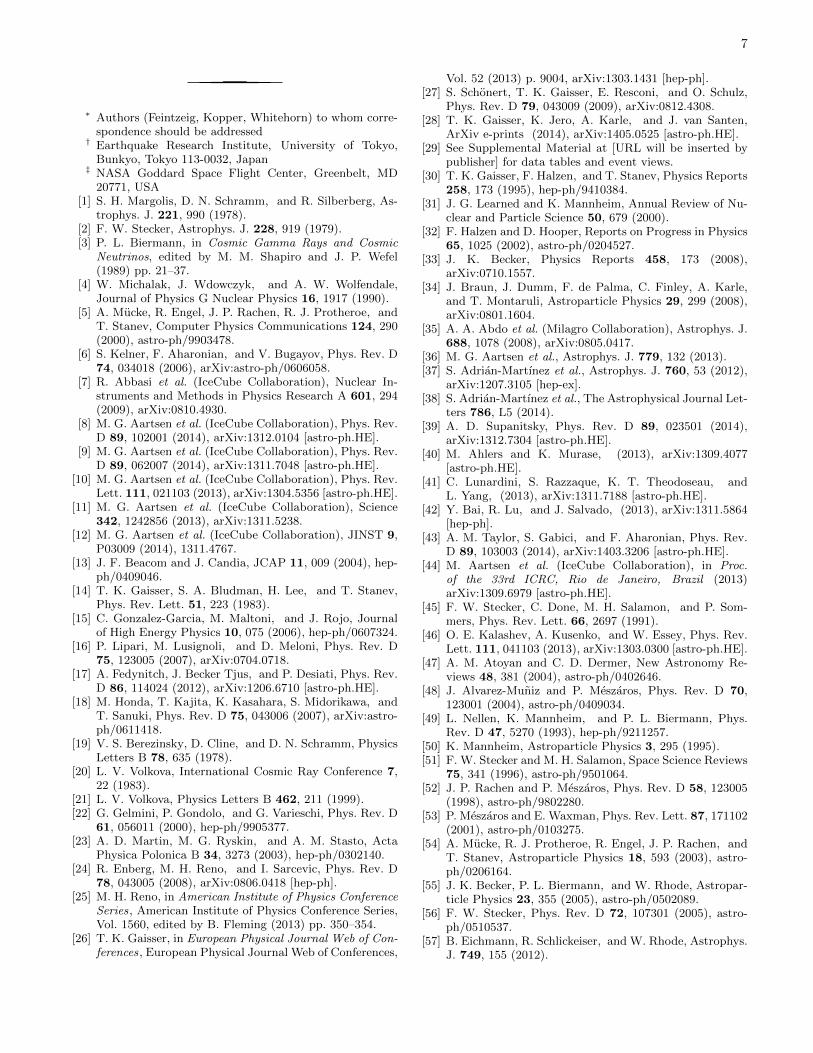
FIG. 3. Arrival angles of events with Edep > 60 TeV, as usedin our fit and above the majority of the cosmic ray muon back-ground. The increasing opacity of the Earth to high energyneutrinos is visible at the right of the plot. Vetoing atmo-spheric neutrinos by muons from their parent air showers de-presses the atmospheric neutrino background on the left. Thedata are described well by the expected backgrounds and ahard astrophysical isotropic neutrino flux (gray lines). Col-ors as in Fig. 2. Variations of this figure with other energythresholds are in the online supplement [29].

for maximal robustness. The penetrating muon back-ground was constrained with a Gaussian prior reflectingour veto efficiency measurement. We obtain a best-fitper-flavor astrophysical flux (ν + ν) in this energy rangeof E2φ(E) = 0.95 ± 0.3 × 10−8 GeV cm−2 s−1 sr−1 andbackground normalizations within the expected ranges.Quoted errors are 1σ uncertainties from a profile like-lihood scan. This model describes the data well, withboth the energy spectrum (Fig. 2) and arrival directions(Fig. 3) of the events consistent with expectations for anorigin in a hard isotropic 1:1:1 neutrino flux. The best-fitatmospheric-only alternative model, however, would re-quire a charm normalization 3.6 times higher than ourcurrent 90% CL upper limit from the northern hemi-sphere νµ spectrum [9]. Even this extreme scenario isdisfavored by the energy and angular distributions of theevents at 5.7σ using a likelihood ratio test.

Fig. 4 shows a fit using a more general model in whichthe astrophysical flux is parametrized as a piecewise func-tion of energy rather than a continuous unbroken E−2

power law. As before, we assume a 1:1:1 flavor ratio andisotropy. While the reconstructed spectrum is compati-ble with our earlier E−2 ansatz, an unbroken E−2 fluxat our best-fit level predicts 3.1 additional events above2 PeV (a higher energy search [10] also saw none). Thismay indicate, along with the slight excess in lower en-ergy bins, either a softer spectrum or a cutoff at highenergies. Correlated systematic uncertainties in the firstfew points in the reconstructed spectrum (Fig. 4) arisefrom the poorly constrained level of the charm atmo-spheric neutrino background. The presence of this softer(E−2.7) component would decrease the non-atmospheric

5

0.0

0.5

1.0

1.5

2.0

2.5

3.0

3.5

4.0E

2 νdNν/dEν [

10−

8G

eVcm

−2s−

1sr−

1]

105 106 107 108

Neutrino Energy [GeV]

Differential Spectrum (best-fit, charm component floats to zero)

Differential Spectrum (fit with charm fixed at IC59 90% C.L.)

FIG. 4. Extraterrestrial neutrino flux (ν + ν) as a functionof energy. Vertical error bars indicate the 2∆L = ±1 con-tours of the flux in each energy bin, holding all other val-ues, including background normalizations, fixed. These pro-vide approximate 68% confidence ranges. An increase in thecharm atmospheric background to the level of the 90% CLlimit from the northern hemisphere νµ spectrum [9] would re-duce the inferred astrophysical flux at low energies to the levelshown for comparison in light gray. The best-fit power law isE2φ(E) = 1.5× 10−8(E/100TeV)−0.3GeVcm−2s−1sr−1.

excess at low energies, hardening the spectrum of the re-maining data. The corresponding range of best fit astro-physical slopes within our current 90% confidence bandon the charm flux [9] is −2.0 to −2.3. As the best-fitcharm flux is zero, the best-fit astrophysical spectrumis on the lower boundary of this interval at −2.3 (solidline, Figs. 2, 3) with a total statistical and systematicuncertainty of ±0.3.

To identify any bright neutrino sources in the data, weemployed the same maximum-likelihood clustering searchas before [11], as well as searched for directional corre-lations with TeV gamma-ray sources. For all tests, thetest statistic (TS) is defined as the logarithm of the ratiobetween the best-fit likelihood including a point sourcecomponent and the likelihood for the null hypothesis, anisotropic distribution [34]. We determined the signifi-cance of any excess by comparing to maps scrambled inright ascension, in which our polar detector has uniformexposure.

As in [11], the clustering analysis was run twice, firstwith the entire event sample, after removing the twoevents (28 and 32) with strong evidence of a cosmic-rayorigin, and second with only the 28 shower events. Thiscontrols for bias in the likelihood fit toward the positionsof single well-resolved muon tracks. We also conductedan additional test in which we marginalize the likelihoodover a uniform prior on the position of the hypotheticalpoint source. This reduces the bias introduced by muons,allowing track and shower events to be used together, andimproves sensitivity to multiple sources by consideringthe entire sky rather than the single best point.

Three tests were performed to search for neutrinos cor-

Galactic

-180 ◦180 ◦

Nor

ther

n H

emis

pher

e

Sou

ther

n H

emis

pher

e

3

12

14

10

25

7

16

5

20

8

1

23

21

2617

19

22

13

9

6

24

11

27

2

4

15

18

29

30

31

3334

35

36

37

0 11.3TS=2log(L/L0)

FIG. 5. Arrival directions of the events in galactic coordi-nates. Shower-like events (median angular resolution ∼ 15◦)are marked with + and those containing muon tracks (. 1◦)with ×. Approximately 40% of the events (mostly tracks[13]) are expected to originate from atmospheric backgrounds.Event IDs match those in the catalog in the online supple-ment [29] and are time ordered. The grey line denotes theequatorial plane. Colors show the test statistic (TS) for thepoint source clustering test at each location. No significantclustering was observed.

related with known gamma-ray sources, also using trackand shower events together. The first two searched forclustering along the galactic plane, with a fixed widthof ±2.5◦, based on TeV gamma-ray measurements [35],and with a free width of between ±2.5◦ and ±30◦. Thelast searched for correlation between neutrino events anda pre-defined catalog of potential point sources (a com-bination of the usual IceCube [36] and ANTARES [37]lists; see online supplement [29]). For the catalog search,the TS value was evaluated at each source location, andthe post-trials significance calculated by comparing thehighest observed value in each hemisphere to results fromperforming the analysis on scrambled datasets.

No hypothesis test yielded statistically significant evi-dence of clustering or correlations. For the all-sky cluster-ing test (Fig. 5), scrambled datasets produced locationswith equal or greater TS 84% and 7.2% of the time forall events and for shower-like events only. As in the two-year data set, the strongest clustering was near the galac-tic center. Other neutrino observations of this locationgive no evidence for a source [38], however, and no newevents were strongly correlated with this region. Whenusing the marginalized likelihood, a test statistic greaterthan or equal to the observed value was found in 28% ofscrambled datasets. The source list yielded p-values forthe northern and southern hemispheres of 28% and 8%,respectively. Correlation with the galactic plane was alsonot significant: when letting the width float freely, thebest fit was ±7.5◦ with a post-trials chance probabilityof 2.8%, while a fixed width of ±2.5◦ returned a p-valueof 24%. A repeat of the time clustering search from [11]

6

also found no evidence for structure.

With or without a possible galactic contribution [39,40], the high galactic latitudes of many of the highest-energy events (Fig. 5) suggest at least some extragalac-tic component. Exception may be made for local largediffuse sources (e.g. the Fermi bubbles [41] or the galac-tic halo [42, 43]), but these models typically can ex-plain at most a fraction of the data. If our data arisefrom an extragalactic flux produced by many isotropi-cally distributed point sources, we can compare our all-sky flux with existing point-source limits. By exploitingthe additional effective volume provided by use of un-contained νµ events, previous point-source studies wouldhave been sensitive to a northern sky point source pro-ducing more than 1-10% of our best-fit flux, dependingon declination and energy spectrum [44]. The lack of anyevidence for such sources from these studies, as well asthe wide distribution of our events, thus lends supportto an interpretation in terms of many individually dimsources. Some contribution from a few comparativelybright sources cannot be ruled out, however, especiallyin the southern hemisphere, where the sensitivity of Ice-Cube to point sources in uncontained νµ is reduced bythe large muon background and small target mass abovethe detector.

The neutrino spectrum (Fig. 4) can also be used to con-strain source properties. In almost all candidate sources[45–69], neutrinos would be produced by the interactionof cosmic rays with either radiation or gas. Interactionswith radiation (pγ) typically produce a peaked spectrum,reflecting the energy spectrum of the photons; those withgas (pp) produce a smooth power law [5, 6]. While pγmodels satisfactorily explain some aspects of the datasuch as the possible drop-off at high energies, many in-volve a central plateau smaller than our observed energyrange, placing them in weak tension with the data. Asan example, the pγ AGN spectrum in [45] peaks at sev-eral PeV with much lower predictions at 100 TeV; thus,while able to explain the highest energy events, it fitspoorly at lower energies and is disfavored as the solesource at the 2σ level with respect to our simple E−2

test flux. Gamma-ray burst pγ models such as [58, 59]have energy ranges better aligned with our data, withcentral plateaus from around 100 TeV to a few PeV, al-though existing limits from searches for correlations withobserved GRBs are more than an order of magnitudebelow the observed flux [70]. Cosmic ray interactionswith gas, such as predicted around supernova remnantsin our and other galaxies, particularly those with highstar-forming rates, produce smooth spectra with slopesreflecting post-diffusion cosmic rays (e.g. E−2.2 in [66])and seem to describe the data well. Large uncertaintieson both the measured neutrino spectrum and all modelsprevent any conclusions, however.

The best-fit flux level in our central energy range(10−8 GeV cm−2 s−1 sr−1 per flavor) is similar to the

Waxman-Bahcall bound [71], the aggregate neutrino fluxfrom charged pion decay in all extragalactic cosmic rayaccelerators if they are optically thin. This bound is de-rived from the cosmic ray spectrum above 1018 eV (1000PeV). Our neutrinos, however, are likely associated withprotons at much lower energies, on the order of 1 to 10PeV [5, 6], at which the bound may be quite different [72].Along with large uncertainties in the neutrino spectrum(Fig. 4), this makes correspondence with the Waxman-Bahcall bound, or 1018 eV cosmic ray sources, unclear.

Further observations with the present or upgraded Ice-Cube detector and the planned KM3NeT [73] telescopeare required to answer many questions about the sourcesof this astrophysical flux [74]. Gamma-ray, optical, andX-ray observations of the directions of individual high-energy neutrinos, which point directly to their origins,may also be able to identify these sources even for thosewith neutrino luminosities too low for identification fromneutrino measurements alone.

We acknowledge support from the following agencies:U.S. National Science Foundation-Office of Polar Pro-grams, U.S. National Science Foundation-Physics Divi-sion, University of Wisconsin Alumni Research Founda-tion, the Grid Laboratory Of Wisconsin (GLOW) gridinfrastructure at the University of Wisconsin - Madi-son, the Open Science Grid (OSG) grid infrastructure;U.S. Department of Energy, and National Energy Re-search Scientific Computing Center, the Louisiana Opti-cal Network Initiative (LONI) grid computing resources;Natural Sciences and Engineering Research Councilof Canada, WestGrid and Compute/Calcul Canada;Swedish Research Council, Swedish Polar Research Sec-retariat, Swedish National Infrastructure for Comput-ing (SNIC), and Knut and Alice Wallenberg Foun-dation, Sweden; German Ministry for Education andResearch (BMBF), Deutsche Forschungsgemeinschaft(DFG), Helmholtz Alliance for Astroparticle Physics(HAP), Research Department of Plasmas with ComplexInteractions (Bochum), Germany; Fund for Scientific Re-search (FNRS-FWO), FWO Odysseus programme, Flan-ders Institute to encourage scientific and technological re-search in industry (IWT), Belgian Federal Science PolicyOffice (Belspo); University of Oxford, United Kingdom;Marsden Fund, New Zealand; Australian Research Coun-cil; Japan Society for Promotion of Science (JSPS); theSwiss National Science Foundation (SNSF), Switzerland;National Research Foundation of Korea (NRF); DanishNational Research Foundation, Denmark (DNRF). Someof the results in this paper have been derived using theHEALPix [75] package. Thanks to R. Laha, J. Beacom,K. Murase, S. Razzaque, and N. Harrington for helpfuldiscussions.

7

∗ Authors (Feintzeig, Kopper, Whitehorn) to whom corre-spondence should be addressed

† Earthquake Research Institute, University of Tokyo,Bunkyo, Tokyo 113-0032, Japan

‡ NASA Goddard Space Flight Center, Greenbelt, MD20771, USA

[1] S. H. Margolis, D. N. Schramm, and R. Silberberg, As-trophys. J. 221, 990 (1978).

[2] F. W. Stecker, Astrophys. J. 228, 919 (1979).[3] P. L. Biermann, in Cosmic Gamma Rays and Cosmic

Neutrinos, edited by M. M. Shapiro and J. P. Wefel(1989) pp. 21–37.

[4] W. Michalak, J. Wdowczyk, and A. W. Wolfendale,Journal of Physics G Nuclear Physics 16, 1917 (1990).

[5] A. Mucke, R. Engel, J. P. Rachen, R. J. Protheroe, andT. Stanev, Computer Physics Communications 124, 290(2000), astro-ph/9903478.

[6] S. Kelner, F. Aharonian, and V. Bugayov, Phys. Rev. D74, 034018 (2006), arXiv:astro-ph/0606058.

[7] R. Abbasi et al. (IceCube Collaboration), Nuclear In-struments and Methods in Physics Research A 601, 294(2009), arXiv:0810.4930.

[8] M. G. Aartsen et al. (IceCube Collaboration), Phys. Rev.D 89, 102001 (2014), arXiv:1312.0104 [astro-ph.HE].

[9] M. G. Aartsen et al. (IceCube Collaboration), Phys. Rev.D 89, 062007 (2014), arXiv:1311.7048 [astro-ph.HE].

[10] M. G. Aartsen et al. (IceCube Collaboration), Phys. Rev.Lett. 111, 021103 (2013), arXiv:1304.5356 [astro-ph.HE].

[11] M. G. Aartsen et al. (IceCube Collaboration), Science342, 1242856 (2013), arXiv:1311.5238.

[12] M. G. Aartsen et al. (IceCube Collaboration), JINST 9,P03009 (2014), 1311.4767.

[13] J. F. Beacom and J. Candia, JCAP 11, 009 (2004), hep-ph/0409046.

[14] T. K. Gaisser, S. A. Bludman, H. Lee, and T. Stanev,Phys. Rev. Lett. 51, 223 (1983).

[15] C. Gonzalez-Garcia, M. Maltoni, and J. Rojo, Journalof High Energy Physics 10, 075 (2006), hep-ph/0607324.

[16] P. Lipari, M. Lusignoli, and D. Meloni, Phys. Rev. D75, 123005 (2007), arXiv:0704.0718.

[17] A. Fedynitch, J. Becker Tjus, and P. Desiati, Phys. Rev.D 86, 114024 (2012), arXiv:1206.6710 [astro-ph.HE].

[18] M. Honda, T. Kajita, K. Kasahara, S. Midorikawa, andT. Sanuki, Phys. Rev. D 75, 043006 (2007), arXiv:astro-ph/0611418.

[19] V. S. Berezinsky, D. Cline, and D. N. Schramm, PhysicsLetters B 78, 635 (1978).

[20] L. V. Volkova, International Cosmic Ray Conference 7,22 (1983).

[21] L. V. Volkova, Physics Letters B 462, 211 (1999).[22] G. Gelmini, P. Gondolo, and G. Varieschi, Phys. Rev. D

61, 056011 (2000), hep-ph/9905377.[23] A. D. Martin, M. G. Ryskin, and A. M. Stasto, Acta

Physica Polonica B 34, 3273 (2003), hep-ph/0302140.[24] R. Enberg, M. H. Reno, and I. Sarcevic, Phys. Rev. D

78, 043005 (2008), arXiv:0806.0418 [hep-ph].[25] M. H. Reno, in American Institute of Physics Conference

Series, American Institute of Physics Conference Series,Vol. 1560, edited by B. Fleming (2013) pp. 350–354.

[26] T. K. Gaisser, in European Physical Journal Web of Con-ferences, European Physical Journal Web of Conferences,

Vol. 52 (2013) p. 9004, arXiv:1303.1431 [hep-ph].[27] S. Schonert, T. K. Gaisser, E. Resconi, and O. Schulz,

Phys. Rev. D 79, 043009 (2009), arXiv:0812.4308.[28] T. K. Gaisser, K. Jero, A. Karle, and J. van Santen,

ArXiv e-prints (2014), arXiv:1405.0525 [astro-ph.HE].[29] See Supplemental Material at [URL will be inserted by

publisher] for data tables and event views.[30] T. K. Gaisser, F. Halzen, and T. Stanev, Physics Reports

258, 173 (1995), hep-ph/9410384.[31] J. G. Learned and K. Mannheim, Annual Review of Nu-

clear and Particle Science 50, 679 (2000).[32] F. Halzen and D. Hooper, Reports on Progress in Physics

65, 1025 (2002), astro-ph/0204527.[33] J. K. Becker, Physics Reports 458, 173 (2008),

arXiv:0710.1557.[34] J. Braun, J. Dumm, F. de Palma, C. Finley, A. Karle,

and T. Montaruli, Astroparticle Physics 29, 299 (2008),arXiv:0801.1604.

[35] A. A. Abdo et al. (Milagro Collaboration), Astrophys. J.688, 1078 (2008), arXiv:0805.0417.

[36] M. G. Aartsen et al., Astrophys. J. 779, 132 (2013).[37] S. Adrian-Martınez et al., Astrophys. J. 760, 53 (2012),

arXiv:1207.3105 [hep-ex].[38] S. Adrian-Martınez et al., The Astrophysical Journal Let-

ters 786, L5 (2014).[39] A. D. Supanitsky, Phys. Rev. D 89, 023501 (2014),

arXiv:1312.7304 [astro-ph.HE].[40] M. Ahlers and K. Murase, (2013), arXiv:1309.4077

[astro-ph.HE].[41] C. Lunardini, S. Razzaque, K. T. Theodoseau, and

L. Yang, (2013), arXiv:1311.7188 [astro-ph.HE].[42] Y. Bai, R. Lu, and J. Salvado, (2013), arXiv:1311.5864

[hep-ph].[43] A. M. Taylor, S. Gabici, and F. Aharonian, Phys. Rev.

D 89, 103003 (2014), arXiv:1403.3206 [astro-ph.HE].[44] M. Aartsen et al. (IceCube Collaboration), in Proc.

of the 33rd ICRC, Rio de Janeiro, Brazil (2013)arXiv:1309.6979 [astro-ph.HE].

[45] F. W. Stecker, C. Done, M. H. Salamon, and P. Som-mers, Phys. Rev. Lett. 66, 2697 (1991).

[46] O. E. Kalashev, A. Kusenko, and W. Essey, Phys. Rev.Lett. 111, 041103 (2013), arXiv:1303.0300 [astro-ph.HE].

[47] A. M. Atoyan and C. D. Dermer, New Astronomy Re-views 48, 381 (2004), astro-ph/0402646.

[48] J. Alvarez-Muniz and P. Meszaros, Phys. Rev. D 70,123001 (2004), astro-ph/0409034.

[49] L. Nellen, K. Mannheim, and P. L. Biermann, Phys.Rev. D 47, 5270 (1993), hep-ph/9211257.

[50] K. Mannheim, Astroparticle Physics 3, 295 (1995).[51] F. W. Stecker and M. H. Salamon, Space Science Reviews

75, 341 (1996), astro-ph/9501064.[52] J. P. Rachen and P. Meszaros, Phys. Rev. D 58, 123005

(1998), astro-ph/9802280.[53] P. Meszaros and E. Waxman, Phys. Rev. Lett. 87, 171102

(2001), astro-ph/0103275.[54] A. Mucke, R. J. Protheroe, R. Engel, J. P. Rachen, and

T. Stanev, Astroparticle Physics 18, 593 (2003), astro-ph/0206164.

[55] J. K. Becker, P. L. Biermann, and W. Rhode, Astropar-ticle Physics 23, 355 (2005), astro-ph/0502089.

[56] F. W. Stecker, Phys. Rev. D 72, 107301 (2005), astro-ph/0510537.

[57] B. Eichmann, R. Schlickeiser, and W. Rhode, Astrophys.J. 749, 155 (2012).

8

[58] E. Waxman and J. Bahcall, Phys. Rev. Lett. 78, 2292(1997).

[59] D. Guetta, D. Hooper, J. Alvarez-Muniz, F. Halzen, andE. Reuveni, Astroparticle Physics 20, 429 (2004).

[60] P. Baerwald, M. Bustamante, and W. Winter, ArXive-prints (2014), arXiv:1401.1820 [astro-ph.HE].

[61] W. Winter, J. Becker Tjus, and S. R. Klein, ArXiv e-prints (2014), arXiv:1403.0574 [astro-ph.HE].

[62] E. Waxman and J. N. Bahcall, Astrophys. J. 541, 707(2000), hep-ph/9909286.

[63] S. Razzaque, P. Meszaros, and E. Waxman, Phys. Rev.D 68, 083001 (2003), astro-ph/0303505.

[64] J. K. Becker, M. Stamatikos, F. Halzen, and W. Rhode,Astroparticle Physics 25, 118 (2006), astro-ph/0511785.

[65] K. Murase and S. Nagataki, Phys. Rev. Lett. 97, 051101(2006), astro-ph/0604437.

[66] A. Loeb and E. Waxman, JCAP 5, 003 (2006), astro-ph/0601695.

[67] K. Murase, M. Ahlers, and B. C. Lacki, Phys. Rev. D88, 121301 (2013), arXiv:1306.3417 [astro-ph.HE].

[68] T. M. Yoast-Hull, J. S. Gallagher, III, E. G. Zweibel,and J. E. Everett, Astrophys. J. 780, 137 (2014),arXiv:1311.5586 [astro-ph.HE].

[69] T. A. Thompson, E. Quataert, E. Waxman, and A. Loeb,Astrophys. J. 654, 219 (2007), astro-ph/0608699.

[70] R. Abbasi et al. (IceCube Collaboration), Nature 484,351 (2012), arXiv:1204.4219 [astro-ph.HE].

[71] E. Waxman and J. Bahcall, Phys. Rev. D 59, 023002(1999), hep-ph/9807282.

[72] K. Mannheim, R. J. Protheroe, and J. P. Rachen, Phys.Rev. D 63, 023003 (2001), astro-ph/9812398.

[73] P. Bagley et al., KM3NeT Technical Design Report for aDeep-Sea Research Infrastructure Incorporating a VeryLarge Volume Neutrino Telescope (KM3NeT Consor-tium, 2011) http://km3net.org/TDR/TDRKM3NeT.pdf.

[74] R. Laha, J. F. Beacom, B. Dasgupta, S. Horiuchi,and K. Murase, Phys. Rev. D 88, 043009 (2013),arXiv:1306.2309 [astro-ph.HE].

[75] K. M. Gorski, E. Hivon, A. J. Banday, B. D. Wandelt,F. K. Hansen, M. Reinecke, and M. Bartelmann, Astro-phys. J. 622, 759 (2005), astro-ph/0409513.

Supplementary Methods and Tables – S1

This section gives additional technical informationabout the result in the main article, including tabularforms of the results, alternative presentations of severalfigures, reviews of referenced methods, and event displaysof the neutrino candidates. Some content is repeatedfrom the main text or from our earlier publication cover-ing the first two years of data [11] for context. Methodsand performance information not provided here (e.g. ef-fective areas) are identical to those in [11]. Event displayshere include only the events first shown in this paper; dis-plays for events 1-28 can be found in the online supple-ment to [11]. Further IceCube data releases can be foundat http://www.icecube.wisc.edu/science/data.

Event Information

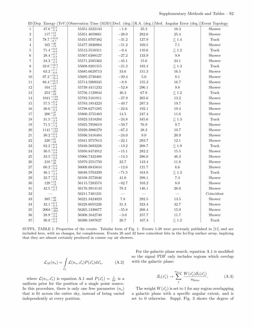
Properties of the 37 neutrino candidate events areshown in Suppl. Tab. I. Five of these (3, 8, 18, 28, 32)contain downgoing muons and have an apparent first in-teraction near the detector boundary and are thereforeconsistent with the expected 8.4± 4.2 background muonevents. Two of these (28 and 32) have subthreshold earlyhits in the veto region, as well as coincident detectionsin the IceTop surface air shower array, and are almostcertainly penetrating cosmic ray muon background. Theremaining events are uniformly distributed throughoutthe detector volume and are consistent with neutrino in-teractions. Their distribution in total PMT charge, usedfor event selection, is shown in Suppl. Fig. 1.

Reconstruction uncertainties given in Suppl. Tab. I in-clude both statistical and systematic uncertainties andwere determined from average reconstruction errors ona population of simulated events of the same topologyin the same part of the detector with similar energiesto those observed. The reconstructions used were maxi-mum likelihood fits of the observed photon timing distri-butions to template events using the cascade and muonloss unfolding techniques described in [12]. Cascade an-gular resolution operates by observing forward/backwardasymmetries in photon timing: in front of the neutrinointeraction, most light is unscattered and arrives over ashort period of time, whereas behind the interaction, thelight has scattered at least once, producing a broader pro-file. Resolution as a function of energy for this analysisis shown in Fig. 14 of [12]. Event 32 is made of two coin-cident cosmic ray muons (see supplemental event views)and so no single energy and direction can be given forthe event.

Point Source Methods

The point source searches used the unbinned maximumlikelihood method from [34]:

10-3

10-2

10-1

100

101

102

103

104

105

106

107

Events

per

988 D

ays

104 105

Total Collected PMT Charge (Photoelectrons)

Charge Threshold

Bkg. Atmospheric Muon Flux (Tagged Data)

Bkg. Atmospheric Neutrinos (π/K)

Bkg. Uncertainties (All Atm. Neutrinos)

Atmospheric Neutrinos (90% CL Charm Limit)

Bkg.+Signal Best-Fit Astrophysical (best-fit slope E−2.3 )

Bkg.+Signal Best-Fit Astrophysical (fixed slope E−2 )

All Events (Trigger Level)

Data

SUPPL. FIG. 1. Distribution of deposited PMT charges(Qtot). Muons at higher total charges are less likely to passthe veto layer undetected, causing the muon background (red,estimated from data) to fall faster than the overall trigger rate(uppermost line). The data events in the unshaded region,at Qtot > 6000, are the events reported in this work. Thehatched region shows current 1σ experimental uncertaintieson both the π/K and prompt components of the atmosphericneutrino background [9]. For scale, the experimental 90%CL upper bound on prompt atmospheric neutrinos [9] is alsoshown (magenta line).

L(ns, ~xs) =

N∏i=1

[nsNSi( ~xs) + (1− ns

N)Bi

]. (A.1)

Here, Bi = 14π represents the isotropic background

probability distribution function (PDF), and the signalPDF Si is the reconstructed directional uncertainty mapfor each event. N is the total number of events inthe data sample and ns is the number of signal events,which is a free parameter. For the all-sky clustering andsource catalog searches, the likelihood is maximized ateach location, resulting in a best-fit # of signal events.Suppl. Fig. 2 shows the arrival directions of the eventsand the result of the point source clustering test in equa-torial coordinates (J2000), while Suppl. Tab. II and IIIlist the results for the 78 sources in the pre-defined cat-alog. This catalog was chosen based on gamma-ray ob-servations or predicted astrophysical neutrino fluxes, andis comprised of sources previously tested by IceCube [36]and ANTARES [37].

To reduce the bias in the likelihood fit towards posi-tions of single well-resolved muon tracks, a marginalizedform of the likelihood was also used for the all-sky test:

Supplementary Methods and Tables – S2

ID Dep. Energy (TeV) Observation Time (MJD) Decl. (deg.) R.A. (deg.) Med. Angular Error (deg.) Event Topology

1 47.6 +6.5−5.4 55351.3222143 −1.8 35.2 16.3 Shower

2 117 +15−15 55351.4659661 −28.0 282.6 25.4 Shower

3 78.7 +10.8−8.7 55451.0707482 −31.2 127.9 . 1.4 Track

4 165 +20−15 55477.3930984 −51.2 169.5 7.1 Shower

5 71.4 +9.0−9.0 55512.5516311 −0.4 110.6 . 1.2 Track

6 28.4 +2.7−2.5 55567.6388127 −27.2 133.9 9.8 Shower

7 34.3 +3.5−4.3 55571.2585362 −45.1 15.6 24.1 Shower

8 32.6 +10.3−11.1 55608.8201315 −21.2 182.4 . 1.3 Track

9 63.2 +7.1−8.0 55685.6629713 33.6 151.3 16.5 Shower

10 97.2 +10.4−12.4 55695.2730461 −29.4 5.0 8.1 Shower

11 88.4 +12.5−10.7 55714.5909345 −8.9 155.3 16.7 Shower

12 104 +13−13 55739.4411232 −52.8 296.1 9.8 Shower

13 253 +26−22 55756.1129844 40.3 67.9 . 1.2 Track

14 1041 +132−144 55782.5161911 −27.9 265.6 13.2 Shower

15 57.5 +8.3−7.8 55783.1854223 −49.7 287.3 19.7 Shower

16 30.6 +3.6−3.5 55798.6271285 −22.6 192.1 19.4 Shower

17 200 +27−27 55800.3755483 14.5 247.4 11.6 Shower

18 31.5 +4.6−3.3 55923.5318204 −24.8 345.6 . 1.3 Track

19 71.5 +7.0−7.2 55925.7958619 −59.7 76.9 9.7 Shower

20 1141 +143−133 55929.3986279 −67.2 38.3 10.7 Shower

21 30.2 +3.5−3.3 55936.5416484 −24.0 9.0 20.9 Shower

22 220 +21−24 55941.9757813 −22.1 293.7 12.1 Shower

23 82.2 +8.6−8.4 55949.5693228 −13.2 208.7 . 1.9 Track

24 30.5 +3.2−2.6 55950.8474912 −15.1 282.2 15.5 Shower

25 33.5 +4.9−5.0 55966.7422488 −14.5 286.0 46.3 Shower

26 210 +29−26 55979.2551750 22.7 143.4 11.8 Shower

27 60.2 +5.6−5.6 56008.6845644 −12.6 121.7 6.6 Shower

28 46.1 +5.7−4.4 56048.5704209 −71.5 164.8 . 1.3 Track

29 32.7 +3.2−2.9 56108.2572046 41.0 298.1 7.4 Shower

30 129 +14−12 56115.7283574 −82.7 103.2 8.0 Shower

31 42.5 +5.4−5.7 56176.3914143 78.3 146.1 26.0 Shower

32 — 56211.7401231 — — — Coincident

33 385 +46−49 56221.3424023 7.8 292.5 13.5 Shower

34 42.1 +6.5−6.3 56228.6055226 31.3 323.4 42.7 Shower

35 2004 +236−262 56265.1338677 −55.8 208.4 15.9 Shower

36 28.9 +3.0−2.6 56308.1642740 −3.0 257.7 11.7 Shower

37 30.8 +3.3−3.5 56390.1887627 20.7 167.3 . 1.2 Track

SUPPL. TABLE I. Properties of the events. Tabular form of Fig. 1. Events 1-28 were previously published in [11] and areincluded here, with no changes, for completeness. Events 28 and 32 have coincident hits in the IceTop surface array, implyingthat they are almost certainly produced in cosmic ray air showers.

LM (ns) =

∫~xs

L(ns, ~xs)P ( ~xs)d ~xs, (A.2)

where L(ns, ~xs) is equation A.1 and P ( ~xs) = 14π is a

uniform prior for the position of a single point source.In this procedure, there is only one free parameter (ns)that is fit across the entire sky, instead of being variedindependently at every position.

For the galactic plane search, equation A.1 is modifiedso the signal PDF only includes regions which overlapwith the galactic plane:

Si( ~xj)→nbins∑j

W ( ~xj)Si( ~xj)nbins

. (A.3)

The weight W ( ~xj) is set to 1 for any region overlappinga galactic plane with a specific angular extent, and isset to 0 otherwise. Suppl. Fig. 3 shows the degree of

Supplementary Methods and Tables – S3

Category Source RA (◦) Dec (◦) ns p-value

SNR TYCHO 6.36 64.18 0.0 –

Cas A 350.85 58.82 0.0 –

IC443 94.18 22.53 0.0 –

W51C 290.75 14.19 0.7 0.05

W44 284.04 1.38 2.5 0.01

W28 270.43 -23.34 4.3 0.01

RX J1713.7-3946 258.25 -39.75 0.0 –

RX J0852.0-4622 133.0 -46.37 0.0 –

RCW 86 220.68 -62.48 0.3 0.41

XB/mqso LSI 303 40.13 61.23 0.0 –

Cyg X-3 308.10 41.23 0.8 0.05

Cyg X-1 299.59 35.20 1.0 0.03

HESS J0632+057 98.24 5.81 0.0 –

SS433 287.96 4.98 1.5 0.02

LS 5039 276.56 -14.83 4.9 0.002

GX 339-4 255.7 -48.79 0.0 –

Cir X-1 230.17 -57.17 0.0 –

Star Form- Cyg OB2 308.10 41.23 0.8 0.05

ation Region

Pulsar/PWN MGRO J2019+37 305.22 36.83 0.9 0.04

Crab Nebula 83.63 22.01 0.0 –

Geminga 98.48 17.77 0.0 –

HESS J1912+101 288.21 10.15 0.8 0.04

Vela X 128.75 -45.6 0.0 –

HESS J1632-478 248.04 -47.82 0.0 –

HESS J1616-508 243.78 -51.40 0.0 –

HESS J1023-575 155.83 -57.76 0.2 0.44

MSH 15-52 228.53 -59.16 0.06 0.48

HESS J1303-631 195.74 -63.52 0.8 0.28

PSR B1259-63 195.74 -63.52 0.8 0.28

HESS J1356-645 209.0 -64.5 0.5 0.35

Galactic Sgr A* 266.42 -29.01 3.1 0.04

Center

Not MGRO J1908+06 286.99 6.27 1.3 0.03

Identified HESS J1834-087 278.69 -8.76 4.7 0.01

HESS J1741-302 265.25 -30.2 2.5 0.07

HESS J1503-582 226.46 -58.74 0.2 0.45

HESS J1507-622 226.72 -62.34 0.1 0.47

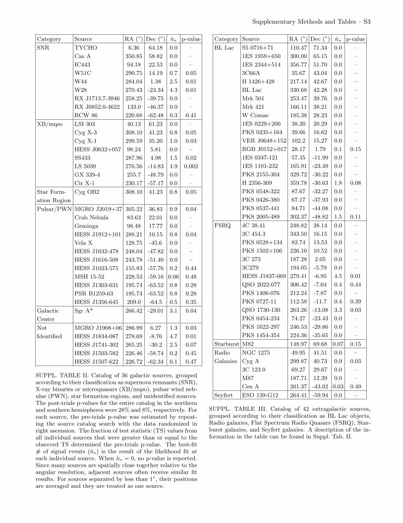
SUPPL. TABLE II. Catalog of 36 galactic sources, groupedaccording to their classification as supernova remnants (SNR),X-ray binaries or microquasars (XB/mqso), pulsar wind neb-ulae (PWN), star formation regions, and unidentified sources.The post-trials p-values for the entire catalog in the northernand southern hemispheres were 28% and 8%, respectively. Foreach source, the pre-trials p-value was estimated by repeat-ing the source catalog search with the data randomized inright ascension. The fraction of test statistic (TS) values fromall individual sources that were greater than or equal to theobserved TS determined the pre-trials p-value. The best-fit# of signal events (ns) is the result of the likelihood fit ateach individual source. When ns = 0, no p-value is reported.Since many sources are spatially close together relative to theangular resolution, adjacent sources often receive similar fitresults. For sources separated by less than 1◦, their positionsare averaged and they are treated as one source.

Category Source RA (◦) Dec (◦) ns p-value

BL Lac S5 0716+71 110.47 71.34 0.0 –

1ES 1959+650 300.00 65.15 0.0 –

1ES 2344+514 356.77 51.70 0.0 –

3C66A 35.67 43.04 0.0 –

H 1426+428 217.14 42.67 0.0 –

BL Lac 330.68 42.28 0.0 –

Mrk 501 253.47 39.76 0.0 –

Mrk 421 166.11 38.21 0.0 –

W Comae 185.38 28.23 0.0 –

1ES 0229+200 38.20 20.29 0.0 –

PKS 0235+164 39.66 16.62 0.0 –

VER J0648+152 102.2 15.27 0.0 –

RGB J0152+017 28.17 1.79 0.1 0.15

1ES 0347-121 57.35 -11.99 0.0 –

1ES 1101-232 165.91 -23.49 0.0 –

PKS 2155-304 329.72 -30.22 0.0 –

H 2356-309 359.78 -30.63 1.8 0.08

PKS 0548-322 87.67 -32.27 0.0 –

PKS 0426-380 67.17 -37.93 0.0 –

PKS 0537-441 84.71 -44.08 0.0 –

PKS 2005-489 302.37 -48.82 1.5 0.11

FSRQ 4C 38.41 248.82 38.14 0.0 –

3C 454.3 343.50 16.15 0.0 –

PKS 0528+134 82.74 13.53 0.0 –

PKS 1502+106 226.10 10.52 0.0 –

3C 273 187.28 2.05 0.0 –

3C279 194.05 -5.79 0.0 –

HESS J1837-069 279.41 -6.95 4.5 0.01

QSO 2022-077 306.42 -7.64 0.4 0.44

PKS 1406-076 212.24 -7.87 0.0 –

PKS 0727-11 112.58 -11.7 0.4 0.39

QSO 1730-130 263.26 -13.08 3.3 0.03

PKS 0454-234 74.27 -23.43 0.0 –

PKS 1622-297 246.53 -29.86 0.0 –

PKS 1454-354 224.36 -35.65 0.0 –

Starburst M82 148.97 69.68 0.07 0.15

Radio NGC 1275 49.95 41.51 0.0 –

Galaxies Cyg A 299.87 40.73 0.9 0.03

3C 123.0 69.27 29.67 0.0 –

M87 187.71 12.39 0.0 –

Cen A 201.37 -43.02 0.03 0.49

Seyfert ESO 139-G12 264.41 -59.94 0.0 –

SUPPL. TABLE III. Catalog of 42 extragalactic sources,grouped according to their classification as BL Lac objects,Radio galaxies, Flat Spectrum Radio Quasars (FSRQ), Star-burst galaxies, and Seyfert galaxies. A description of the in-formation in the table can be found in Suppl. Tab. II.

Supplementary Methods and Tables – S4

Equatorial

0 ◦360 ◦

3

12

14 10

25

7

16

5

20

8

1

2321

26

17

19

22

139

6

2411

27

2

415

18

29

30

31

33

34

35

36

37

0 11.3TS=2log(L/L0)

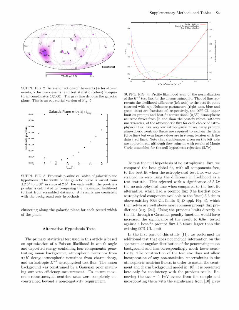
SUPPL. FIG. 2. Arrival directions of the events (+ for showerevents, × for track events) and test statistic (colors) in equa-torial coordinates (J2000). The gray line denotes the galacticplane. This is an equatorial version of Fig. 5.

0 5 10 15 20 25 30

θmax[◦ ]

0.00

0.05

0.10

0.15

0.20

0.25

0.30

0.35

0.40

Pre

-tri

als

p-v

alu

e

Galactic Plane with |b|<θmax

SUPPL. FIG. 3. Pre-trials p-value vs. width of galactic planehypothesis. The width of the galactic plane is varied from±2.5◦ to ±30◦ in steps of 2.5◦. For each width, the pre-trialsp-value is calculated by comparing the maximized likelihoodto that from scrambled datasets. All results are consistentwith the background-only hypothesis.

clustering along the galactic plane for each tested widthof the plane.

Alternative Hypothesis Tests

The primary statistical test used in this article is basedon optimization of a Poisson likelihood in zenith angleand deposited energy containing four components: pene-trating muon background, atmospheric neutrinos fromπ/K decay, atmospheric neutrinos from charm decay,and an isotropic E−2 astrophysical test flux. The muonbackground was constrained by a Gaussian prior match-ing our veto efficiency measurement. To ensure maxi-mum robustness, all neutrino rates were completely un-constrained beyond a non-negativity requirement.

1σ

2σ

3σ

4σ

5σ

6σ

0 0.5 1 1.5 2 2.5 3 0

0.5

1

1.5

2

2.5

3

3.5

4

-∆2ln

(L)

Nuis

ance P

ara

mete

r V

alu

e

E-2

x 10-8

GeV cm-2

s-1

sr-1

Profile LikelihoodBest-fit Conventional Scaling

Best-fit Charm Scaling

SUPPL. FIG. 4. Profile likelihood scan of the normalizationof the E−2 test flux for the unconstrained fit. The red line rep-resents the likelihood difference (left axis) to the best-fit point(marked with ×). Nuisance parameters (right axis, blue andgreen lines) are fractions of, respectively, the 90% CL upperlimit on prompt and best-fit conventional (π/K) atmosphericneutrino fluxes from [9] and show the best-fit values, withoutuncertainties, of the atmospheric flux for each choice of astro-physical flux. For very low astrophysical fluxes, large promptatmospheric neutrino fluxes are required to explain the data(blue line) but even large values are in strong tension with thedata (red line). Note that significances given on the left axisare approximate, although they coincide with results of MonteCarlo ensembles for the null hypothesis rejection (5.7σ).

To test the null hypothesis of no astrophysical flux, wecompared the best global fit, with all components free,to the best fit when the astrophysical test flux was con-strained to zero using the difference in likelihood as atest statistic. This rejected with a significance of 5.7σthe no-astrophysical case when compared to the best-fitalternative, which had a prompt flux (the hardest non-astrophysical component available to the fitter) 3.6 timesabove existing 90% CL limits [9] (Suppl. Fig. 4), whichthemselves are well above most common prompt flux pre-dictions (e.g. [24]). Using the previous limits directly inthe fit, through a Gaussian penalty function, would haveincreased the significance of the result to 6.8σ, testedagainst a best-fit prompt flux 1.6 times larger than theexisting 90% CL limit.

In the first part of this study [11], we performed anadditional test that does not include information on thespectrum or angular distribution of the penetrating muonbackground and has correspondingly much lower sensi-tivity. The construction of the test also does not allowincorporation of any non-statistical uncertainties in theatmospheric neutrino fluxes, in order to match the treat-ment and charm background model in [10]; it is presentedhere only for consistency with the previous result. Re-moving the two ∼ 1 PeV events from the sample andincorporating them with the significance from [10] gives

Supplementary Methods and Tables – S5

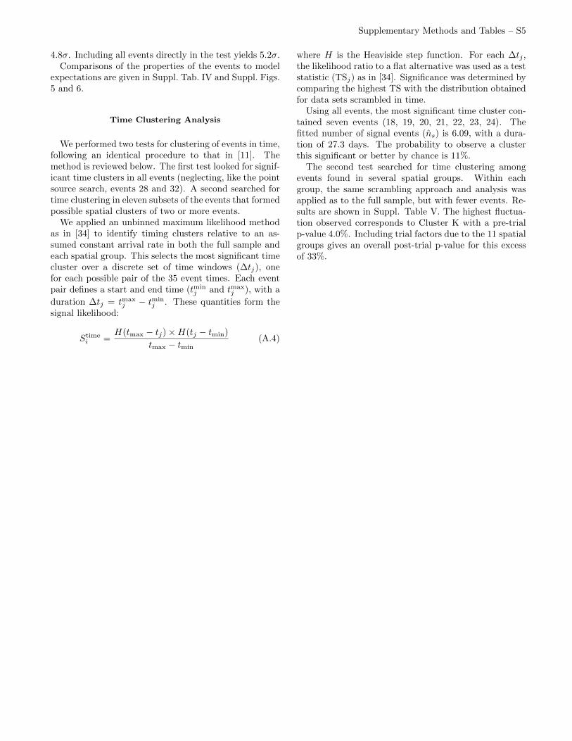
4.8σ. Including all events directly in the test yields 5.2σ.Comparisons of the properties of the events to model

expectations are given in Suppl. Tab. IV and Suppl. Figs.5 and 6.

Time Clustering Analysis

We performed two tests for clustering of events in time,following an identical procedure to that in [11]. Themethod is reviewed below. The first test looked for signif-icant time clusters in all events (neglecting, like the pointsource search, events 28 and 32). A second searched fortime clustering in eleven subsets of the events that formedpossible spatial clusters of two or more events.

We applied an unbinned maximum likelihood methodas in [34] to identify timing clusters relative to an as-sumed constant arrival rate in both the full sample andeach spatial group. This selects the most significant timecluster over a discrete set of time windows (∆tj), onefor each possible pair of the 35 event times. Each eventpair defines a start and end time (tmin

j and tmaxj ), with a

duration ∆tj = tmaxj − tmin

j . These quantities form thesignal likelihood:

Stimei =

H(tmax − tj)×H(tj − tmin)

tmax − tmin(A.4)

where H is the Heaviside step function. For each ∆tj ,the likelihood ratio to a flat alternative was used as a teststatistic (TSj) as in [34]. Significance was determined bycomparing the highest TS with the distribution obtainedfor data sets scrambled in time.

Using all events, the most significant time cluster con-tained seven events (18, 19, 20, 21, 22, 23, 24). Thefitted number of signal events (ns) is 6.09, with a dura-tion of 27.3 days. The probability to observe a clusterthis significant or better by chance is 11%.

The second test searched for time clustering amongevents found in several spatial groups. Within eachgroup, the same scrambling approach and analysis wasapplied as to the full sample, but with fewer events. Re-sults are shown in Suppl. Table V. The highest fluctua-tion observed corresponds to Cluster K with a pre-trialp-value 4.0%. Including trial factors due to the 11 spatialgroups gives an overall post-trial p-value for this excessof 33%.

Supplementary Methods and Tables – S6

10-1

100

101

Events

per

988 D

ays

1.0 0.5 0.0 0.5 1.0sin(Declination)

Northern Sky (upgoing)Southern Sky (downgoing)

Edep > 0 TeV

10-1

100

101

Events

per

988 D

ays

1.0 0.5 0.0 0.5 1.0sin(Declination)

Northern Sky (upgoing)Southern Sky (downgoing)

Edep > 30 TeV

10-1

100

101

Events

per

988 D

ays

1.0 0.5 0.0 0.5 1.0sin(Declination)

Edep > 50 TeV

10-1

100

101

Events

per

988 D

ays

1.0 0.5 0.0 0.5 1.0sin(Declination)

Edep > 60 TeV

10-1

100

101

Events

per

988 D

ays

1.0 0.5 0.0 0.5 1.0sin(Declination)

Edep > 70 TeV

10-1

100

101

Events

per

988 D

ays

1.0 0.5 0.0 0.5 1.0sin(Declination)

Edep > 80 TeV

10-1

100

101

Events

per

988 D

ays

1.0 0.5 0.0 0.5 1.0sin(Declination)

Edep > 90 TeV

10-1

100

101

Events

per

988 D

ays

1.0 0.5 0.0 0.5 1.0sin(Declination)

Edep > 100 TeV

10-1

100

101

Events

per

988 D

ays

1.0 0.5 0.0 0.5 1.0sin(Declination)

Edep > 200 TeV

10-1

100

101

Events

per

988 D

ays

1.0 0.5 0.0 0.5 1.0sin(Declination)

Edep > 300 TeV

Background Atmospheric Muon Flux

Atmospheric Neutrinos (90% CL Charm Limit)

Data

Bkg. Atmospheric Neutrinos (π/K)

Bkg.+Signal Best-Fit Astrophysical (best-fit slope E−2.3 )

Background Uncertainties

Bkg.+Signal Best-Fit Astrophysical (fixed slope E−2 )

SUPPL. FIG. 5. Expected and observed distribution of events in declination for various cuts in deposited energy. The solidgray line (E−2.3 added to backgrounds) provides a better fit to the data than the E−2 benchmark (dashed) at the 1σ level.

Supplementary Methods and Tables – S7

all energies

Muons π/K atm. ν Prompt atm. ν E−2 (best-fit) E−2.3 (best-fit) Sum (E−2) Sum (E−2.3) Data

Tot. Events 8.4± 4.2 6.6+2.2−1.6 < 9.0 (90% CL) 23.8 23.7 38.8 38.7 37 (36)

Up 0 4.2 < 6.1 8.3 9.4 12.4 13.5 9

Down 8.4 2.4 < 2.9 15.5 14.4 26.3 25.2 27

Track ∼ 7.6 4.5 < 1.7 4.6 4.3 16.7 16.4 8

Shower ∼ 0.8 2.1 < 7.2 19.2 19.5 22.1 22.4 28

Fraction Up 0% 63% 68% 35% 40% 32% 35% 25%

Fraction Down 100% 37% 32% 65% 60% 68% 65% 75%

Fraction Tracks > 90% 69% 19% 19% 18% 43% 42% 24%

Fraction Showers < 10% 31% 81% 81% 82% 57% 58% 76%

Edep < 60 TeV

Muons π/K atm. ν Prompt atm. ν E−2 (best-fit) E−2.3 (best-fit) Sum (E−2) Sum (E−2.3) Data

Tot. Events 8.0 4.2 < 3.7 2.2 3.8 14.5 16.1 16

Up 0 2.6 < 2.4 1.2 2.0 3.7 4.7 4

Down 8.0 1.6 < 1.3 1.1 1.8 10.7 11.4 12

Track ∼ 7.2 2.9 < 0.7 0.4 0.6 10.5 10.7 4

Shower ∼ 0.8 1.4 < 3.0 1.8 3.2 4.0 5.3 12

Fraction Up 0% 63% 65% 52% 53% 26% 29% 25%

Fraction Down 100% 37% 35% 48% 47% 74% 71% 75%

Fraction Tracks > 90% 68% 19% 19% 17% 72% 67% 25%

Fraction Showers < 10% 32% 81% 81% 83% 28% 33% 75%

60 TeV < Edep < 3 PeV

Muons π/K atm. ν Prompt atm. ν E−2 (best-fit) E−2.3 (best-fit) Sum (E−2) Sum (E−2.3) Data

Tot. Events 0.4 2.4 < 5.3 18.2 18.6 21.0 21.4 20

Up 0 1.5 < 3.7 6.7 7.2 8.2 8.7 5

Down 0.4 0.8 < 1.6 11.6 11.4 12.8 12.7 15

Track ∼ 0.4 1.7 < 1.0 3.8 3.5 5.8 5.5 4

Shower ∼ 0.0 0.7 < 4.2 14.4 15.1 15.2 15.8 16

Fraction Up 0% 64% 70% 37% 39% 39% 41% 25%

Fraction Down 100% 36% 30% 63% 61% 61% 59% 75%

Fraction Tracks > 90% 71% 20% 21% 19% 28% 26% 20%

Fraction Showers < 10% 29% 80% 79% 81% 72% 74% 80%

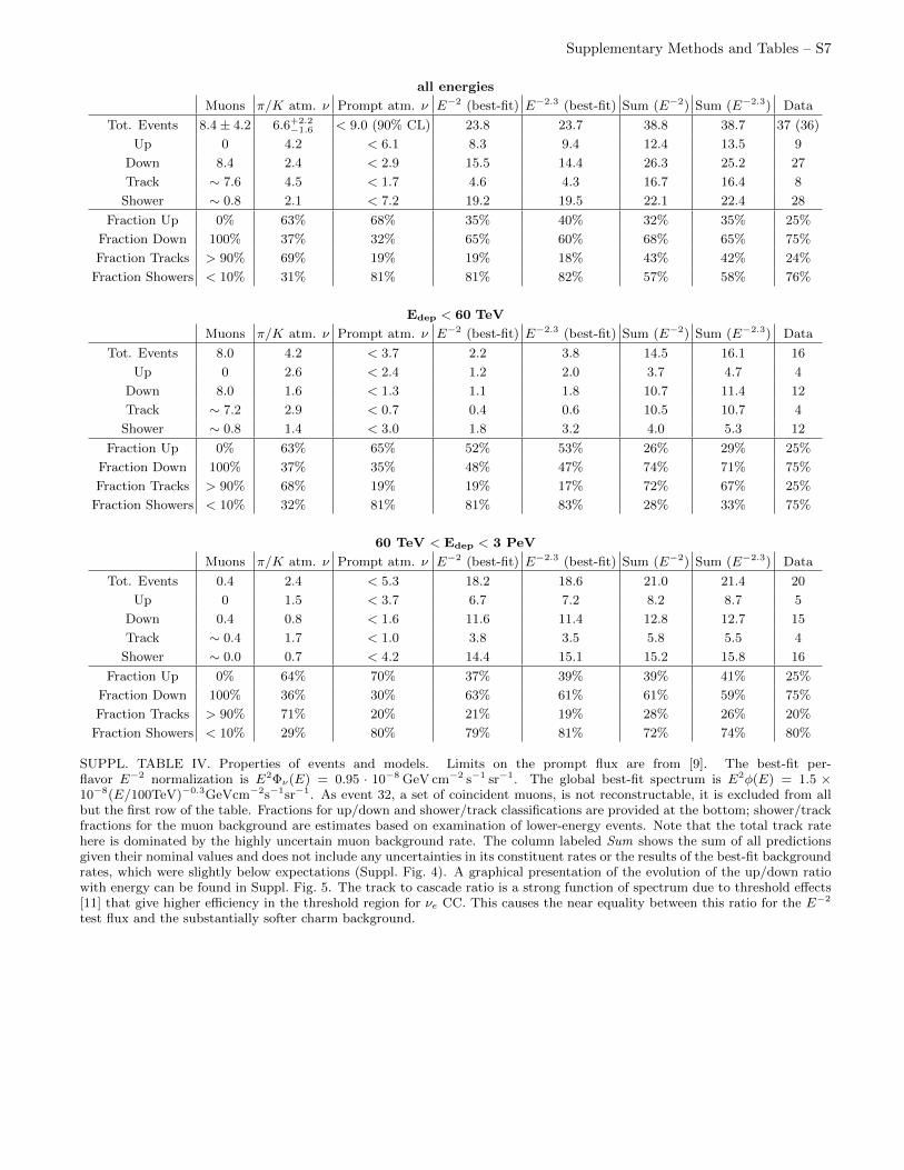
SUPPL. TABLE IV. Properties of events and models. Limits on the prompt flux are from [9]. The best-fit per-flavor E−2 normalization is E2Φν(E) = 0.95 · 10−8 GeV cm−2 s−1 sr−1. The global best-fit spectrum is E2φ(E) = 1.5 ×10−8(E/100TeV)−0.3GeVcm−2s−1sr−1. As event 32, a set of coincident muons, is not reconstructable, it is excluded from allbut the first row of the table. Fractions for up/down and shower/track classifications are provided at the bottom; shower/trackfractions for the muon background are estimates based on examination of lower-energy events. Note that the total track ratehere is dominated by the highly uncertain muon background rate. The column labeled Sum shows the sum of all predictionsgiven their nominal values and does not include any uncertainties in its constituent rates or the results of the best-fit backgroundrates, which were slightly below expectations (Suppl. Fig. 4). A graphical presentation of the evolution of the up/down ratiowith energy can be found in Suppl. Fig. 5. The track to cascade ratio is a strong function of spectrum due to threshold effects[11] that give higher efficiency in the threshold region for νe CC. This causes the near equality between this ratio for the E−2

test flux and the substantially softer charm background.

Supplementary Methods and Tables – S8

10-1

100

101

102

Events

per

988 D

ays

wit

h d

eposi

ted E

> 6

0 T

eV

1.0 0.5 0.0 0.5 1.0sin(Declination)

Northern Sky (upgoing)Southern Sky (downgoing)

Background Atmospheric Muon Flux

Bkg. Atmospheric Neutrinos (π/K)

Atmospheric Neutrinos (90% CL Charm Limit)

Atmospheric Neutrinos (90% CL Charm Limit) [assuming no veto]

Bkg.+Signal Best-Fit Astrophysical (best-fit slope E−2.3 )

Bkg.+Signal Best-Fit Astrophysical (fixed slope E−2 )

Data

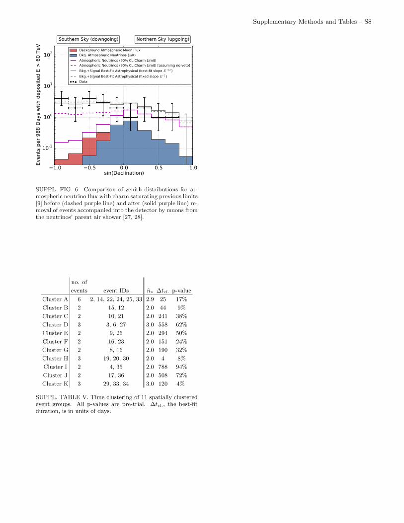
SUPPL. FIG. 6. Comparison of zenith distributions for at-mospheric neutrino flux with charm saturating previous limits[9] before (dashed purple line) and after (solid purple line) re-moval of events accompanied into the detector by muons fromthe neutrinos’ parent air shower [27, 28].

no. of

events event IDs ns ∆tcl. p-value

Cluster A 6 2, 14, 22, 24, 25, 33 2.9 25 17%

Cluster B 2 15, 12 2.0 44 9%

Cluster C 2 10, 21 2.0 241 38%

Cluster D 3 3, 6, 27 3.0 558 62%

Cluster E 2 9, 26 2.0 294 50%

Cluster F 2 16, 23 2.0 151 24%

Cluster G 2 8, 16 2.0 190 32%

Cluster H 3 19, 20, 30 2.0 4 8%

Cluster I 2 4, 35 2.0 788 94%

Cluster J 2 17, 36 2.0 508 72%

Cluster K 3 29, 33, 34 3.0 120 4%

SUPPL. TABLE V. Time clustering of 11 spatially clusteredevent groups. All p-values are pre-trial. ∆tcl., the best-fitduration, is in units of days.

Supplementary Methods and Tables – S9

EVENT 29

0.0 0.3 0.6 0.9 1.2 1.5 1.8 2.1 2.4 2.7 3.0

Time [microseconds]

Deposited Energy (TeV) Time (MJD) Declination (deg.) RA (deg.) Med. Ang. Resolution (deg.) Topology

32.7 +3.2−2.9 56108.2572046 41.0 298.1 7.4 Shower

Supplementary Methods and Tables – S10

EVENT 30

0.0 0.3 0.6 0.9 1.2 1.5 1.8 2.1 2.4 2.7 3.0

Time [microseconds]

Deposited Energy (TeV) Time (MJD) Declination (deg.) RA (deg.) Med. Ang. Resolution (deg.) Topology

129 +14−12 56115.7283574 −82.7 103.2 8.0 Shower

Supplementary Methods and Tables – S11

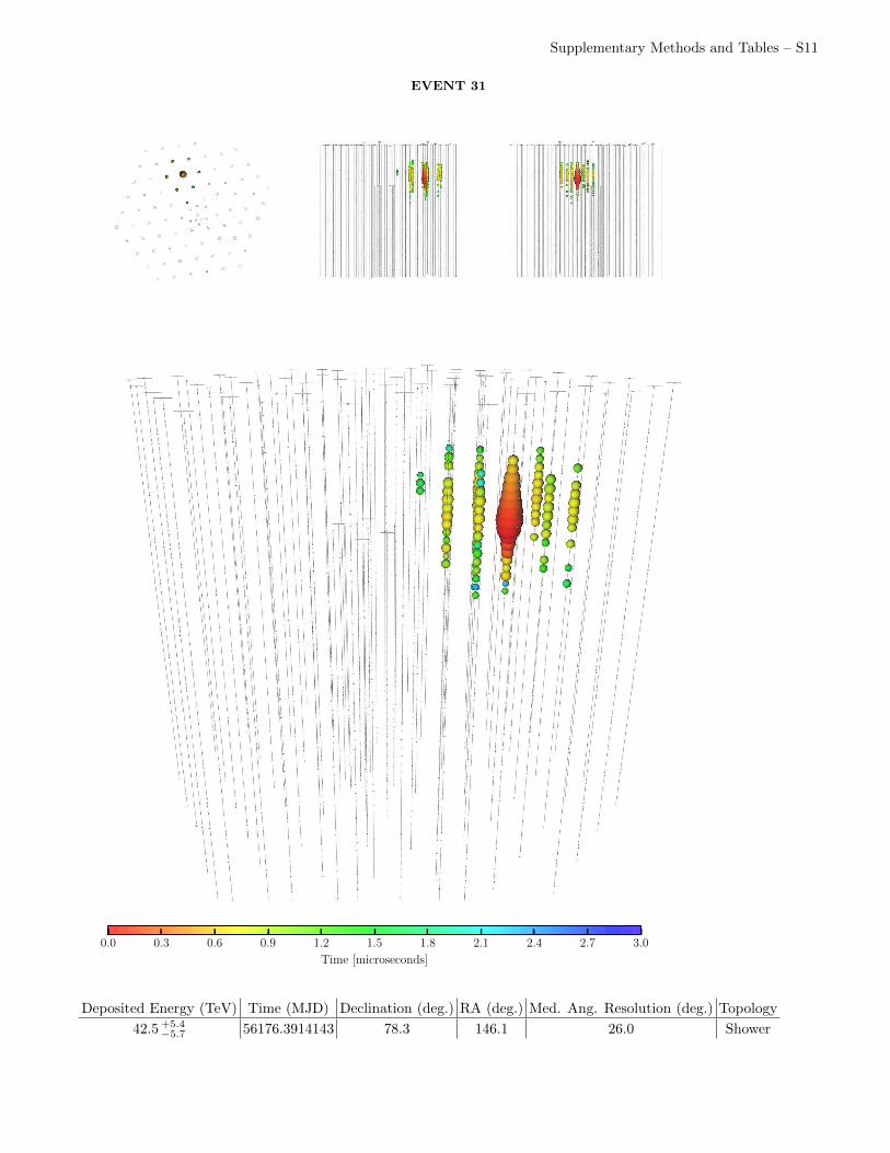
EVENT 31

0.0 0.3 0.6 0.9 1.2 1.5 1.8 2.1 2.4 2.7 3.0

Time [microseconds]

Deposited Energy (TeV) Time (MJD) Declination (deg.) RA (deg.) Med. Ang. Resolution (deg.) Topology

42.5 +5.4−5.7 56176.3914143 78.3 146.1 26.0 Shower

Supplementary Methods and Tables – S12

EVENT 32

0.0 0.3 0.6 0.9 1.2 1.5 1.8 2.1 2.4 2.7 3.0

Time [microseconds]

Deposited Energy (TeV) Time (MJD) Declination (deg.) RA (deg.) Med. Ang. Resolution (deg.) Topology

— 56211.7401231 — — — Coincident

Supplementary Methods and Tables – S13

EVENT 33

0.0 0.3 0.6 0.9 1.2 1.5 1.8 2.1 2.4 2.7 3.0

Time [microseconds]

Deposited Energy (TeV) Time (MJD) Declination (deg.) RA (deg.) Med. Ang. Resolution (deg.) Topology

385 +46−49 56221.3424023 7.8 292.5 13.5 Shower

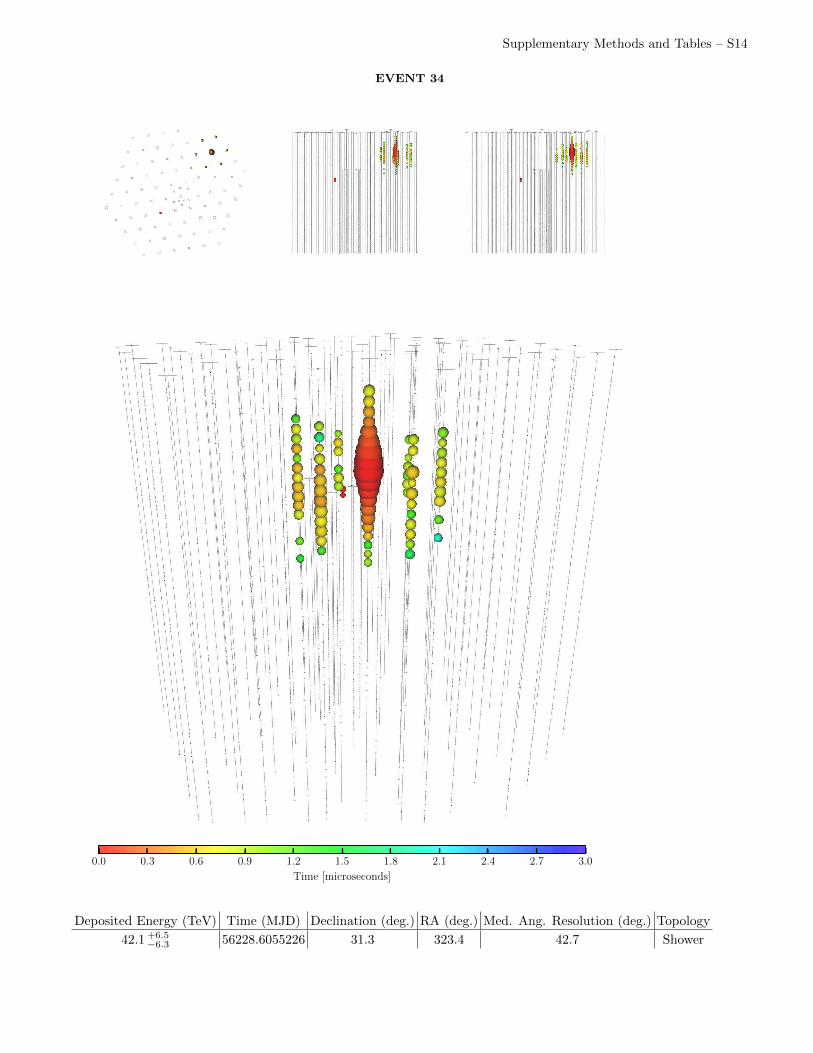
Supplementary Methods and Tables – S14

EVENT 34

0.0 0.3 0.6 0.9 1.2 1.5 1.8 2.1 2.4 2.7 3.0

Time [microseconds]

Deposited Energy (TeV) Time (MJD) Declination (deg.) RA (deg.) Med. Ang. Resolution (deg.) Topology

42.1 +6.5−6.3 56228.6055226 31.3 323.4 42.7 Shower

Supplementary Methods and Tables – S15

EVENT 35

0.0 0.3 0.6 0.9 1.2 1.5 1.8 2.1 2.4 2.7 3.0

Time [microseconds]

Deposited Energy (TeV) Time (MJD) Declination (deg.) RA (deg.) Med. Ang. Resolution (deg.) Topology

2004 +236−262 56265.1338677 −55.8 208.4 15.9 Shower

Supplementary Methods and Tables – S16

EVENT 36

0.0 0.3 0.6 0.9 1.2 1.5 1.8 2.1 2.4 2.7 3.0

Time [microseconds]

Deposited Energy (TeV) Time (MJD) Declination (deg.) RA (deg.) Med. Ang. Resolution (deg.) Topology

28.9 +3.0−2.6 56308.1642740 −3.0 257.7 11.7 Shower

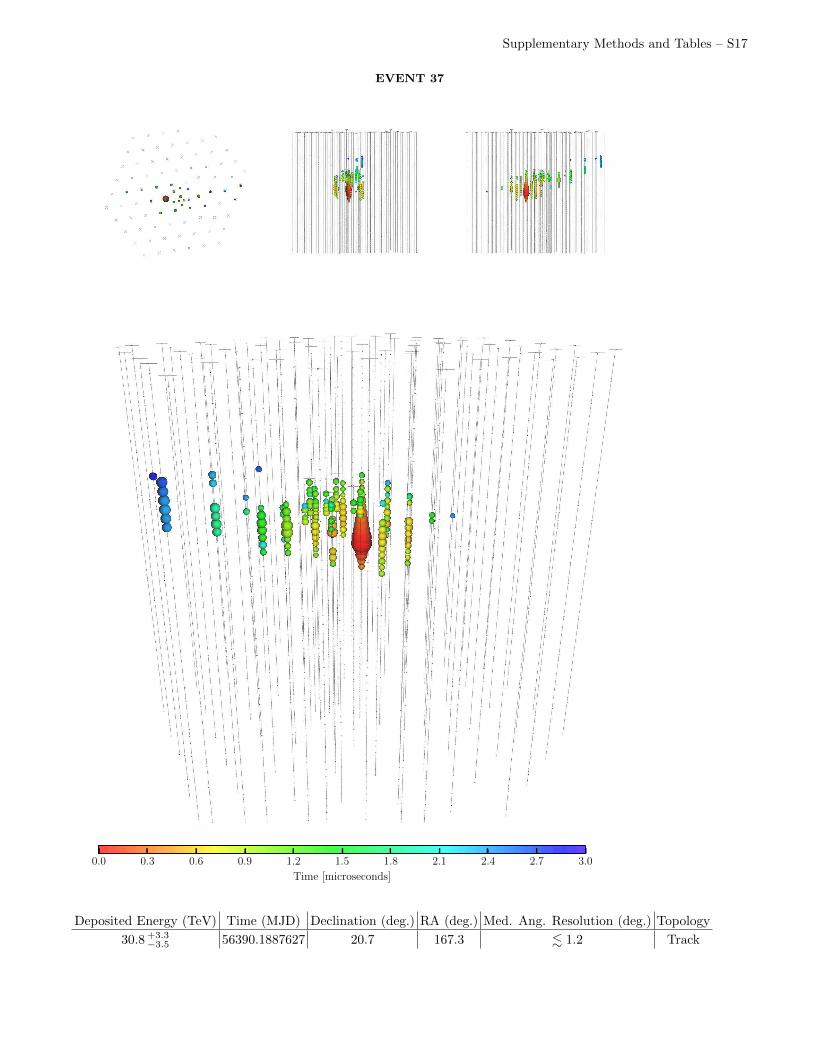
Supplementary Methods and Tables – S17

EVENT 37

0.0 0.3 0.6 0.9 1.2 1.5 1.8 2.1 2.4 2.7 3.0

Time [microseconds]

Deposited Energy (TeV) Time (MJD) Declination (deg.) RA (deg.) Med. Ang. Resolution (deg.) Topology

30.8 +3.3−3.5 56390.1887627 20.7 167.3 . 1.2 Track