OBJECT RECOGNITION USING

SHAPE AND BEHAVIORAL

FEATURES

by

Chetan Bhole

A thesis submitted to the

Faculty of the Graduate School

of the

State University of New York at Buffalo

in partial fulfillment of the requirements for the

degree of Master of Science

Department of Computer Science and Engineering

August 18, 2006

Abstract

Object Recognition is the domain of computer vision that deals with the

classification of objects in two or three dimensions as instances of predeter-

mined object classes, and is useful for image analysis and understanding.

One of the most powerful properties used for recognition of objects is the

shape of the object. Other features traditionally used include color, texture,

moments and other attributes visible from single static images. The diffi-

culty in obtaining error-free classification is that image data almost always

has noise, is cluttered with many different objects and the objects may be

occluded or hidden so only a fraction of the object is visible. That is why

it is useful to consider additional information which is not available from

single static images.

In this thesis we define and employ behavioral features along with shape

features to characterize objects. We model the dynamic behavior of each

object class by its common pattern of movement to help disambiguate dif-

ferent objects that may look similar but belong to different object classes

in light of their distinct behavioral features. We show that for a simulated

environment problem where we create a database of a mix of objects with

small and large variations in shapes, sizes and behavior models, the error

rate of the system that uses shape alone decreases from a top-choice error

rate of 7-30% to a top-choice error rate of 2-3% using shape and behavioral

features, with performance gain with the addition of behavioral features de-

pending on the noise levels in cases where the shapes are similar but objects

have different behaviors.

1

ACKNOWLEDGMENT

I take this opportunity to sincerely thank my advisor Dr. Peter D. Scott

for his guidance in this work. His valuable ideas and suggestions went a long

way in elucidating many of the key concepts I have used and the discussions

I have had with him are the cornerstones that helped me complete my the-

sis. For this, I would like to give complete credit to him.

I would like to thank Dr. Matthew J. Beal of the State University of

New York at Buffalo for sparing his valuable time to be a part of my thesis

committee.

I am grateful to Dr. Rutao Yao of the State University of New York at

Buffalo for supporting and encouraging me to work on the thesis.

I am indebted to my parents, my brother Harshal and his wife Swapna. If

it hadn’t been for them I would not have been here to do this thesis. Their

moral support will continue to drive me in my future endeavors too. I am

grateful to Rahul Krishna for his insightful discussions which helped shed

light on some of the problems I encountered during this thesis. Thanks go

to my roommates Amol Kothari, Ketan Shenoy and Mukul Patil for their

constant encouragement and for reviewing part of this material. Last, but

not the least, I would also like to thank all my friends who supported me in

every aspect during this work.

Thank you.

2

Contents

1 Introduction and Problem Statement 8

1.1 Background . . . . . . . . . . . . . . . . . . . . . . . . . . . . 8

1.2 Objective . . . . . . . . . . . . . . . . . . . . . . . . . . . . . 8

1.3 Scope . . . . . . . . . . . . . . . . . . . . . . . . . . . . . . . 9

1.4 Limitations . . . . . . . . . . . . . . . . . . . . . . . . . . . . 12

2 Overview of Object Recognition 14

2.1 Literature review . . . . . . . . . . . . . . . . . . . . . . . . . 14

2.2 Shape: recognition from static images . . . . . . . . . . . . . 15

2.3 Behavior: dynamic aspects of recognition . . . . . . . . . . . 16

2.4 Combining shape and behavioral cues . . . . . . . . . . . . . 16

3 Background 18

3.1 B-splines . . . . . . . . . . . . . . . . . . . . . . . . . . . . . 18

3.1.1 Introduction . . . . . . . . . . . . . . . . . . . . . . . 18

3.1.2 Preliminaries . . . . . . . . . . . . . . . . . . . . . . . 19

3.1.3 Uniform cubic B-spline . . . . . . . . . . . . . . . . . . 20

3.1.4 Translational, rotational and scaling invariance . . . . 24

3.1.5 End conditions and multiple vertices . . . . . . . . . . 24

3.1.6 Closed curves . . . . . . . . . . . . . . . . . . . . . . . 24

3.2 Particle filters . . . . . . . . . . . . . . . . . . . . . . . . . . . 26

3.2.1 Introduction to particle filtering . . . . . . . . . . . . 26

3.2.2 Kalman filter . . . . . . . . . . . . . . . . . . . . . . . 27

3.2.3 Non-Linear filters . . . . . . . . . . . . . . . . . . . . . 28

3.2.4 Particle filters . . . . . . . . . . . . . . . . . . . . . . . 29

3

3.2.5 Condensation algorithm . . . . . . . . . . . . . . . . . 31

3.3 Syntactic parsing rules . . . . . . . . . . . . . . . . . . . . . . 34

3.4 Classifiers . . . . . . . . . . . . . . . . . . . . . . . . . . . . . 36

3.4.1 Artificial neural networks . . . . . . . . . . . . . . . . 36

4 Design Methodology 42

4.1 Conceptual design of the classifier system . . . . . . . . . . . 42

4.2 Stepping through the system operation . . . . . . . . . . . . . 47

5 Environment Setup and Test Cases 50

5.1 Object Shapes and Paths . . . . . . . . . . . . . . . . . . . . 50

5.2 Grammar rules . . . . . . . . . . . . . . . . . . . . . . . . . . 53

5.3 ORMOT . . . . . . . . . . . . . . . . . . . . . . . . . . . . . . 54

5.4 Test data generation . . . . . . . . . . . . . . . . . . . . . . . 54

5.5 Parameters . . . . . . . . . . . . . . . . . . . . . . . . . . . . 58

5.6 Test cases . . . . . . . . . . . . . . . . . . . . . . . . . . . . . 60

6 Results 61

7 Conclusions and Future work 74

7.1 Conclusions . . . . . . . . . . . . . . . . . . . . . . . . . . . . 74

7.2 Future work . . . . . . . . . . . . . . . . . . . . . . . . . . . . 75

4

List of Figures

1.1 Flight patterns . . . . . . . . . . . . . . . . . . . . . . . . . . 10

3.1 Curve . . . . . . . . . . . . . . . . . . . . . . . . . . . . . . . 19

3.2 Approximate B-spline . . . . . . . . . . . . . . . . . . . . . . 20

3.3 Piecewise linear curve . . . . . . . . . . . . . . . . . . . . . . 21

3.4 B-spline curve . . . . . . . . . . . . . . . . . . . . . . . . . . . 22

3.5 Basis functions . . . . . . . . . . . . . . . . . . . . . . . . . . 22

3.6 Four basis functions . . . . . . . . . . . . . . . . . . . . . . . 23

3.7 Multiple control vertices . . . . . . . . . . . . . . . . . . . . . 25

3.8 Collinear control vertices . . . . . . . . . . . . . . . . . . . . . 25

3.9 Closed curve . . . . . . . . . . . . . . . . . . . . . . . . . . . 26

3.10 Condensation algorithm . . . . . . . . . . . . . . . . . . . . . 33

3.11 Derivation tree . . . . . . . . . . . . . . . . . . . . . . . . . . 35

3.12 Perceptron . . . . . . . . . . . . . . . . . . . . . . . . . . . . 37

3.13 Multilayer neural network . . . . . . . . . . . . . . . . . . . . 40

4.1 Work engine . . . . . . . . . . . . . . . . . . . . . . . . . . . . 43

5.1 Objects . . . . . . . . . . . . . . . . . . . . . . . . . . . . . . 52

5.2 First screen of ORMOT . . . . . . . . . . . . . . . . . . . . . 55

5.3 Second screen of ORMOT . . . . . . . . . . . . . . . . . . . . 56

5.4 Third screen of ORMOT . . . . . . . . . . . . . . . . . . . . . 57

5.5 Data Generation . . . . . . . . . . . . . . . . . . . . . . . . . 58

6.1 Tracked corners of objects . . . . . . . . . . . . . . . . . . . . 62

6.2 Tracked corners of objects with more noise . . . . . . . . . . . 63

6.3 Averaged object shapes . . . . . . . . . . . . . . . . . . . . . 63

5

6.4 True path of type 2 . . . . . . . . . . . . . . . . . . . . . . . . 64

6.5 Path of type 1 . . . . . . . . . . . . . . . . . . . . . . . . . . 65

6.6 Smoothed path of type 11 . . . . . . . . . . . . . . . . . . . . 66

6.7 Smoothed path of type 2 . . . . . . . . . . . . . . . . . . . . . 67

6.8 Smoothed path of type 10 . . . . . . . . . . . . . . . . . . . . 68

6

List of Tables

6.1 NN training Table . . . . . . . . . . . . . . . . . . . . . . . . 69

6.2 Accuracy Table 1 . . . . . . . . . . . . . . . . . . . . . . . . . 69

6.3 Accuracy Table 2 . . . . . . . . . . . . . . . . . . . . . . . . . 70

6.4 Accuracy Table 3 . . . . . . . . . . . . . . . . . . . . . . . . . 70

6.5 Accuracy Table 4 . . . . . . . . . . . . . . . . . . . . . . . . . 71

6.6 Accuracy Table 5 . . . . . . . . . . . . . . . . . . . . . . . . . 71

6.7 Accuracy Table 6 . . . . . . . . . . . . . . . . . . . . . . . . . 72

6.8 Accuracy Table 7 . . . . . . . . . . . . . . . . . . . . . . . . . 72

6.9 Accuracy Table 8 . . . . . . . . . . . . . . . . . . . . . . . . . 73

6.10 Accuracy Table 9 . . . . . . . . . . . . . . . . . . . . . . . . . 73

7

Chapter 1

Introduction and Problem

Statement

1.1 Background

Object recognition is the process by which a system, biological or artificial,

tries to classify or identify an object. In computer vision this identification

has been done using different cues the most prominent of which has been

shape, others being color, texture, moments, topology, etc. In most problem

settings, shape is definitely one of the strongest cues that help identify the

object. Typically, other cues help in identifying the object faster or favor

approximate answers in case of shape ambiguities. For example, consider a

purple apple - the human mind will be able to make out that the object has

the shape of an apple (provided the shape of the object can be recognized)

but the color is different from that of an apple. Shape, the dominant cue,

persuades us that it is indeed an apple, albeit one with an unusual color.

1.2 Objective

Shape can be observed from static imagery. When video imagery is available,

one can observe how the object moves over space and time. The dynamic

characteristics that are associated with a given object class constitute its

behavior. Behavior can be used as another cue to help identify an object.

8

This cue is particularly useful when the object cannot be seen clearly or

the shape cannot adequately discriminate to provide us the information we

need. It is critical to predetermine the behavioral pattern of the object to

be identified if we have to use this cue, just as we must know the shape

characteristics of an object class to use shape cues to aid recognition. The

behavioral pattern can be converted to features which can be used, alone

or in conjunction with shape features, to train the system to recognize the

object.

1.3 Scope

Let us consider examples where the behavior cues could be useful for object

recognition in order to illustrate why behavior is an important cue.

1. Consider a scenario where you are watching birds at some distance.

Your task is to identify which bird is which type. For example, an

ornithologist may require a labeled video or images indicating the bird

types for his studies. If the birds look similar or are at some distance

away so that the shape cannot be used effectively to classify the birds,

we can still use their motion behaviors, sound or color to recognize

them. Different species of birds do have characteristic motion patterns

when observed closely as is illustrated in the Figure 1.1. These could be

used to identify or classify the birds. Consider flight patterns identified

at the Cornell Lab of Ornithology as shown. The report from which

this figure is extracted further notes that ways of identifying birds

include shape, field marks, posture, size, flight pattern and habitat.

Besides the flight pattern, the posture can also be considered as a

behavioral pattern.

2. It is often necessary, and sometimes critical, to distinguish various

classes of aircraft by their radar returns: military, commercial pas-

senger, cargo, or general aviation aircraft, and if military, fighter-

interceptor, bomber or specialized counter-measure aircraft. Radar

returns often do not contain adequate information to distinguish shape

features sufficient to make the recognition. But a highly maneuver-

9

Figure 1.1: The different flight patterns of birds.

10

able fighter, for instance, can be easily distinguished from a lumbering

bomber or wide-body passenger aircraft by its flight pattern. Simple

behavioral cues such as airspeed can immediately disambiguate a jet

aircraft from a single engine general aviation vehicle.

3. A similar example to differentiating between varieties of birds is to dif-

ferentiate between different fish in the sea or between different schools

of fish using their swim pattern. One would also be able to differentiate

between different fish species which move at different speeds. Hence it

can be possible to differentiate between a blue shark and the shortfin

mako shark that moves faster in water. In addition, some species such

as sharks swim with a side-to-side rhythmic motion, while others such

as dolphins use an up-down rhythmic motion.

4. It would be possible to differentiate between whales and submarines

through their motion and turns they take during movement.

5. During a day of heavy snow or rain, it is likely that the movement of

a human may help us identify that it is a human as opposed to an

animal. The snow or rain can distort the shape information.

6. Each person has a characteristic way of walking. When closely ob-

served, this behavior can be used to some degree to help identify the

person from a distance or from behind, and hence used as a biometric

feature [1].

7. Consider a courier collecting and distributing packages in a locality.

After observing that the person is going to several houses with boxes

should give a cue as to what this person is doing and hence who he

may be i.e. a courier. Here the shape information will be useless and

it will become more difficult to identify the person type if the person

is not clad in a recognizable uniform.

8. Consider a supermarket. We need to identify the shoplifters from the

authentic shoppers. It will not be possible to differentiate between

these classes unless we note what each of the individuals in the shop is

doing. The shoplifter will be behaving in surreptitious ways, such as

11

putting things in his pockets without placing them back on the rack or

in the cart. Nothing in shape or geometry could identify the shoplifter.

Thus behavioral cues would be essential to disambiguate the normal

shopper from the shoplifter [2], [3].

These are some of the examples where behavior can be used as an im-

portant cue that will aid in computer vision based object recognition. We

discuss in our study the nature of behavioral cues, and how to extract be-

havioral features that can be used to support object recognition.

1.4 Limitations

Behavior cannot always be of great value in object recognition. There are

limitations to the use of behavioral cues as well as favorable situations. Some

common scenario characteristics that do not rely on behavior to recognize

an object are:

1. The objects are stationary. A tree cannot be discriminated from a

telephone pole by their behaviors.

2. Both the object types have same or similar behaviors. Actually, sta-

tionary behavior is a specific behavior, and item one above is a special

case of this item. A fish can be discriminated from a rock in a stream

by the rock’s stationary behavior.

3. Objects don’t follow the behavior pattern that was used to train the

system. A shoplifter may behave as a legitimate shopper while he or

she is in range of a security camera.

4. The behavior may be occluded by objects in front of it.

5. The shape and other features are so prominent that behavior may be

unnecessary.

Hence when designing the object recognition system, we do not claim

that behavior features are always necessary or even useful. But when video

data is available, there are many circumstances in which behavior of object

12

classes can be modeled and recognition systems benefit by training to use

behavioral cues in visual object recognition.

13

Chapter 2

Overview of Object

Recognition

2.1 Literature review

Object Recognition deals with the recognition or classification of different

objects in two or three dimensional images as instances of predetermined

object classes. Object recognition is useful for image analysis and under-

standing. Shape [4] has been used as one of the most powerful features

to recognize the object. There are other features that are also used like

color [4],[5], texture [5], depth, topology, moments [6],[7], etc. that are de-

rived from static images. More complex Bayesian methods and aspect graph

methods are also used. Image data almost always has noise, is cluttered with

many different objects and the objects may be occluded or hidden so only a

fraction of the part is visible. Besides this the object may be present in any

location, orientation and may be scaled in the image. Different parts of the

image and hence the object may be illuminated differently and by different

light sources. Considering all this variation and a multitude of possibilities

would cause recognition systems to have high computational complexity,

high decision latency and be vulnerable to error. Ideally, the recognition

system should have scale, translation and rotation invariant algorithms, be

robust to occlusions, noise and illumination differences, should be capable of

capturing the containment relationship of parts of an object and should be

14

fast enough to be useful for use for real time applications. The system could

also have specialized algorithms running in parallel for detecting specific

features needed to enhance the performance of the system.

A lot of research has been done in object recognition. Different shape

techniques are used for object recognition. [4] combines shape and color

information for object recognition. [8] uses shape-from-shading techniques.

Similarly shape-from-texture exist [5]. [9] uses shape contexts for shape

matching. [10] uses wavelet transforms for shape matching that can be used

for object recognition. [11] uses shape similarity aspect graphs. Shapes

of the objects are not rigid and can change. Taking care of this change is

discussed in [12]. [13] discusses how to use shadow shape curves for 3 dimen-

sional object recognition. The most basic shape features for two dimensional

objects are discussed in [14].

2.2 Shape: recognition from static images

We consider the simple shape features that are used for 2D objects that

are discussed in [14]. Some of these shape features include the moments

of different orders. They include the boundary length, area and moment

of inertia. The compactness of the object is derived from the area and

boundary length. The number of holes in the object is also a property of

the object. The area and boundary length are shape and rotation invariant

but not scale invariant. Hence it would be necessary to normalize the image

if these properties are to be used. The moment of inertia about the x, y and

xy is also a useful property. To re-orient the object to a standard, the object

can be rotated using the axis of minimum moment of inertia about xy. This

can be done if the object is not symmetrical or if the ambiguities regarding

more than 1 minimum values can be resolved. B-splines [15] can represent

the shape of the object and after standardization of the object i.e. rotating

and shifting to the origin, the coefficients can be used as shape properties.

15

2.3 Behavior: dynamic aspects of recognition

Behavior may be defined as the action or reaction of an object or organism

usually in relation to the environment [16]. It can be conscious or uncon-

scious, overt or covert and voluntary or involuntary [16]. The behavior we

are interested in is that kind that is characteristic of specific object classes,

which can be observed, and which can be used for training. Objects may

move in characteristic patterns of movement. Such a type of behavior can

be observed in many animals like the bees [17]. Quite some amount of work

has been done to classify humans using the gait and periodicity [18], [19], [1].

Periodicity as a behavior has been exploited in most of the work [19], [20],

[2], [21], [22]. Most of the strategies have been the use of hidden Markov

models and classification of trajectories [19], [23], [18]. Also motion patterns

have been extracted in the frequency domain as discussed in [24].

We don’t want to restrict ourselves to periodic motion as a method of

detection of behavior. Behavioral features can consist of ordered sequences

of brief movements referred to as gestures, and gestures can in turn consist of

lower level more primitive movements. For example for a bird that makes a

wavy motion followed by 3 loops in the air as its characteristic behavior, we

can say that the wavy motion is a high level gesture and a sequence of 3 loops

is another high level gesture. The lower level behavior will consist of the

small left or right turns it makes or the straight line motion. These sequenced

gestures make up the dynamic aspects that may help characterize objects

and hence can be employed as behavioral features useful for recognition of

certain objects.

2.4 Combining shape and behavioral cues

Most of the object recognition systems documented in the literature rely on

static features alone. In fact the shape features are used for tracking the

objects [25]. Behavior in itself can aid in classification in cases where the

objects have some particular distinguishable pattern but have noisy shape

features or very similar shape features in which case the shape and behav-

ior features can be combined to improve the performance of the system.

16

Demonstrating this by the design and testing of a recognition system which

combines shape and behavioral features is the main research goal of this

thesis.

17

Chapter 3

Background

In this chapter background material critical to the design methodology devel-

oped in the remainder of the thesis is briefly reviewed. Much fuller treatment

of these topics is available in the cited references.

3.1 B-splines

Spline shapes contain the curves of minimum strain energy and hence are

considered mechanically sound. They give better performance in shape mod-

eling than polylines connecting points and other families of curves, and are

the representational framework for modeling the bounding contours of ob-

jects employed in this study.

3.1.1 Introduction

For curve drawing, we can either interpolate the curve so that the curve goes

through all the points or approximate the curve where a limit is defined to

the distance between curves and points and hence the curve does not go

through all the points. If we would connect the points by lines instead of

curves, it would result in irregularities, discontinuities of derivatives, waste

of space for storage and difficulty in manipulation. In splines a curve is

defined by piecing together a succession of curve segments hence it is termed

as a ‘piecewise’ approach[15]. Interpolation is easier than approximation

but lacks some desirable properties. Bezier introduced the technique of

18

Figure 3.1: The curve Q showing umin and umax.

approximating using user-defined control points. Parametric B-splines have

the advantage that we can control the degree of smoothness (continuity of

derivatives) at the joints between adjacent curve segments independent of

the order of the segments and number of control points. This level of control

is not possible using Bezier curves, and motivates the use of B-splines to

approximating the bounding contours for shape description.

3.1.2 Preliminaries

For a 2 dimensional curve, we can write the equation [15] of the curve as

Q(u) = (X(u), Y (u)). (3.1)

X and Y are single valued denoting the x and y co-ordinates. Similarly for a

3 dimensional curve we can add Z that will denote the z co-ordinates. The

Figure 3.1 shows a curve with its parameter u. A single curve for X(u) and

another for Y (u) will not produce a satisfactory curve. Hence we break the

curve into a number of pieces called segments each defined by separate poly-

nomials and join the segments to form a piecewise polynomial curve. Hence

from the path of umin to umax, we get certain values of u called knots that are

the joints between the polynomial segments u0, u1, . . . umin, . . . umax, . . . ulast

which is the knot sequence or knot vector and ui ≤ ui+1 always. There is

one polynomial piece between each uj and uj+1 for X(u) and Y (u).

The continuity constraints at the joints are important. If 0th to dth

derivative are everywhere continuous along the entire curve including the

joints [15], then X and Y are said to be Cd continuous. Sometimes there are

19

Figure 3.2: The approximate B-spline curve is shown with a few of the knot

positions. The dashed lines show the sequence of control points used to

create the B-spline curve.

multiple knots at the same point (ui = ui+1) that cause the interval [ui, ui+1]

to be vacuous for issues of continuity. However sometimes we will have all

knots as distinct and a constant or uniform distance apart ui+1 = ui +δ and

it is termed as a uniform knot sequence.

3.1.3 Uniform cubic B-spline

The B-spline is a curve created using the approximation method [15]. The

uniform cubic B-spline has a uniform knot sequence and each segment is

represented by a cubic polynomial. This spline has local control i.e. altering

the position of a single data point (control vertex) causes only a part of the

curve to change. This is computationally advantageous since we don’t have

to recompute the position of the entire curve if we only change a few points.

The sequence of control vertices forms the control graph or control polygon.

A piecewise linear curve is shown in the Figure 3.3. In this the line

connects the control vertices. The equation [15] for such a curve can be

written as

Qi(u) = (Xi(u), Yi(u))

= (1− u)vi−1 + uvi

where v can be replaced by x for the x-coordinate equations and y for the

y-coordinate equations. So changing Vi affects only Qi(u) and Qi+1(u). vi−1

20

Figure 3.3: This is a piecewise linear curve where the control points are

connected by straight lines.

and vi scale a unit hat function whose max height is 1. In other words vi−1

and vi is weighted by a corresponding unit hat function. The values of u

are non-negative values and hence act as weights. vs on the other hand can

have any positive, negative or zero value like scale factors. We can write the

equations [15] as

Vi(u) = vi−1Bi−1(u) + viBi(u) for ui ≤ u < ui+1 (3.2)

where

Bi(u) =u− ui

ui+1 − uifor ui ≤ u < ui+1

=ui+2 − u

ui+2 − ui+1for ui+1 ≤ u < ui+2

Hence at any point, that point is a linear combination of the functions Bi or

as a weighted sum of the control vertices vi. The unit hat functions Bi(u)

are called basis functions. vi contributes to the curve only where Bi(u) is

non-zero. Since for vi, Bi(u) is non-zero over [ui, ui+1) and [ui+1, ui+2),

vi can influence only Qi(u) and Qi+1(u). So in general we can write the

equation of the curve [15] as

Q(u) =∑

i

viBi(u)

=∑

i

(xiBi(u), yiBi(u)).

21

Figure 3.4: The curve figure shows the B-spline curve with the Q parts of

the curve and the control graph.

Figure 3.5: This figure shows the basis function with its four parts.

The basis functions for the piecewise cubic polynomial B-spline are shown

in the Fig. 3.5. These are not scaled. They get scaled appropriately by the

control vertices.

For control vertices 0 to m we need 4 basis functions to define the cubic

curve segment i.e. there are 3 more control vertices than curve segments.

In short, for m+1 control vertices, there are m+1 basis functions, m-2 curve

segments bounded by m-1 knots and m−1+3+3 = m+5 knots altogether.

The curve is generated as u runs from u3 to um+1 with the conditions u0 <

u1 < u2 < u3 = umin; umin = u3 < u4 < u5 . . . < um+1 = umax ; umax =

um+1 < um+2 < um+3 < um+4. B(u) consists of 4 basis segments b−0(u),

b−1(u), b−2(u), b−3(u) and each segment has the coefficients of the cubic

22

Figure 3.6: Four basis functions with their labels. The bold red section is

the part that will be responsible for creation of one of the segment of the

curve.

polynomial a, b, c and d. We need to determine 16 coefficients to determine

B(u). Also Bi(u) = 0 for u ≤ ui and u ≥ ui+4. So the 1st and 2nd

derivatives B1i (u) and B2

i (u) are zero outside (ui, ui+4). Also the first and

second derivatives match at each knot uj . We solve the equations [15] to

give us the following results

b−0(u) =16u3 (3.3)

b−1(u) =16(1 + 3u + 3u2 − 3u3) (3.4)

b−2(u) =16(4− 6u2 + 3u3) (3.5)

b−3(u) =16(1− 3u + 3u2 − u3) (3.6)

To determine a curve, we select a set of control vertices Vi and use them to

define the curve given by the equation Q(u) =∑

i ViBi(u) and each Bi is

simply a copy of B, shifted so that it extends from ui to ui+4.

Qi(u) =r=0∑

r=−3

Vi+rBi+r(u)

= Vi−3Bi−3(u) + Vi−2Bi−2(u) + Vi−1Bi−1(u) + ViBi(u).

Replacing Bj(u) by the particular segment that pertains to the interval

23

[ui, ui+1), we get the equation [15]

Qi(u) =r=0∑

r=−3

Vi+rbr(u)

= Vi−3b−3(u) + Vi−2b−2(u) + Vi−1b−1(u) + Vib−0(u).

and is shown in the figure. Overall, for a uniform cubic B-spline, we have 3

fewer segments than we have control vertices.

3.1.4 Translational, rotational and scaling invariance

It is a desirable property that if we would shift or change the position of

all control vertices by the same amount it would not affect the shape of the

curve. This comes naturally to the curve and can be shown [15]. Similarly

another desirable property is that if we would rotate all control vertices by

the same amount it would not affect the shape of the curve. This also comes

naturally to the curve and can be shown [15]. The scaling invariance is very

similar to rotational invariance. Together they are equivalent to invariance

under affine transformations.

3.1.5 End conditions and multiple vertices

To control the end control vertices, we can either repeat the end vertices

V0 and Vm or create phantom vertices where ever we want so as to control

the shape of the curve and can label those control points as V−1 and Vm+1.

If we use multiple end vertices the shape of the curve changes depending

on the number of multiple end vertices used. For example using 2 repeated

end vertices causes the curve at the end to have a zero curvature while

for 3 repeated end points, the curve interpolates between those end points

(Figure 3.7). If 3 consecutive control points are collinear, then the curve

passes through the middle control point as depicted in the Figure 3.8. If 4

consecutive control points are collinear, then the curve between the second

and the third control point is a straight line as shown in the Figure 3.8.

3.1.6 Closed curves

If we repeat the first 3 vertices as the last 3 vertices of the control vector [15],

the curve obtained becomes closed and continuous. This can be observed

24

Figure 3.7: The effect of having multiple control vertices at the same point

is seen in this figure.

Figure 3.8: (a) The curve passes through the control vertex if the 3 consec-

utive control vertices are collinear.(b) The curve becomes a line through 2

control vertices if 4 consecutive control vertices are collinear.

25

Figure 3.9: This is an example of a closed curve by repeating the first 3

vertices as the last 3 vertices in the control vector.

from the fact that Pstart = V0+4V1+V26 and Pend = Vm+1+4Vm+2+Vm+3

6 which

turns out to be the same as the Pstart equation. The Figure 3.9 shows such

a closed curve.

3.2 Particle filters

3.2.1 Introduction to particle filtering

Stochastic filtering deals with estimating the distribution of a process given

data up to the current time point [26]. If we use Bayesian statistics and

Bayes rule for inference this filtering is called Bayesian filtering. We can

estimate what the internal state xn is, given the observations y0:n with the

goal of maximizing the a posteriori probability of our estimate. Stochastic

filtering is often implemented recursively, updating the estimate of state at

one time to the next time. In the case that the update is based on the

current observation, this is referred to as recursive stochastic state filtering.

Recursive stochastic state filtering [27] may be generalized to the re-

cursive estimation of state using only observations up to some earlier time

(prediction), or up to some later time (smoothing).

1. Filtering : estimating the current state xn given estimates of the previ-

26

ous states x0:n−1 and the current and previous observations y0:n using

process and measurement models

2. Prediction: (estimating a future state xn′>n given earlier state esti-

mates x0:n and observations y0:n

3. Smoothing : finding xn′<n given state estimates x0:n and y0:n

The stochastic filtering problem in a dynamic state-space form [27] can

be given by

1. State equation:

xn = f(n, xn−1, un, dn) (3.7)

where d denotes the process noise in the system and u denotes the

system input vector in a controlled environment. The current internal

state is a function of the current time, the previous internal state, the

input vector (if in a controlled environment) and the process noise.

2. Measurement equation:

yn = g(n, xn, un, vn) (3.8)

where u denotes the system input vector in a controlled environment

and v denotes the measurement noise. The observed state thus de-

pends on the current time, the current internal state, the input control

vector and the noise.

These equations reduce to the following if we neglect the input control

vector:

xn = f(xn−1, dn) (3.9)

yn = g(xn, vn) (3.10)

3.2.2 Kalman filter

The Kalman filter [27], [28] is an optimal (minimum mean square error

among its peers) recursive (needs previous data for predicting current state)

data processing algorithm (filter) and used for a linear dynamic system with

27

the system having Gaussian noise (the probability density function has a

bell shaped curve). The equations above reduce to

xn+1 = Fn+1,nxn + dn (3.11)

yn = Gnxn + vn (3.12)

Fn+1,n is the transition matrix while moving from state n to n+1, Gn is

measurement matrix in the current state and vn and dn are the noise in the

system.

The Kalman filter [27] consists of the iterative predictor-corrector steps:

1. Time update: one step prediction of the measurement.

2. Measurement update: correction of the time update state estimate by

propagating the conditional density given the observation.

The first order statistics (mean) and second order statistics (variance) fully

determine a Gaussian density and the Kalman filter propagates both these

(hence all information) without error to the next step. Note the optimality

of the Kalman filter is limited to the linear Gaussian case.

3.2.3 Non-Linear filters

For non-linear or linear but non-Gaussian filtering [27], no closed form exact

optimal solution can in general be obtained, the solution is infinite dimen-

sional and hence the need to approximate. Approximate solutions to the

nonlinear filtering problem have two categories: global methods (numerical

approximation techniques used) and the local methods (linearization tech-

niques or finite sum approximation).

The classes of non-linear filters can be enumerated [27] as:

1. Linearization method filters: Extended Kalman filter where the state

equation and measurement equation are linearized and the posterior

p(xn|y0:n) approximated as a Gaussian.

2. Finite-Dimensional filters: Can be applied when the observations and

filtering densities belong to the exponential class. This is usually per-

formed with the conjugate approach where the prior and posterior are

28

assumed to come from some parametric probability function family.

e.g. Daum filter, Benes filter and projection filter.

3. Classic partial differential equations (PDE) methods

4. Spectral Methods

5. Neural filter Methods

6. Particle Filters

The numerical approximation methods [27] include Gaussian/Laplace

approximation, iterative quadrature, multigrid method and point-mass ap-

proximation, moment approximation, gaussian sum approximation, deter-

ministic sampling approximation and Monte Carlo sampling approximation.

As the power of digital computers grow, non-linear non-Gaussian stochas-

tic approximations based on sampling distributions which promise accuracy

and robustness but at the cost of increased computational complexity have

become attractive in many applications. In order to reduce the computation

needs (associated with higher dimensionality and higher order moments), we

need to represent the pdf as a set of random samples rather than a function

over state space. For this purpose the sequential Monte Carlo methods [27]

are used. Sequential Monte Carlo methods are used for parameter estimation

(system identification) and state estimation (particle filters). Different kinds

of Monte Carlo sampling methods exist that include importance sampling,

rejection sampling, sequential importance sampling, sequential importance

resampling (SIR), stratified sampling, Markov Chain Monte Carlo, Hybrid

Monte-Carlo and Quasi Monte-Carlo. SIR in particular involves a resam-

pling step inserted between two importance sampling steps to eliminate the

samples with small importance weights and duplicate the samples with big

weights thereby rejuvenating the sampler.

3.2.4 Particle filters

Sequential Monte Carlo is a kind of recursive Bayesian filter based on Monte

Carlo simulation and is also called bootstrap filter. The working of the

particle filter [27] can be summarized as follows:

29

The state space is partitioned as many parts, in which the particles are

selected according to some probability measure with higher probability re-

gions indicating more concentration of particles. The particle system evolves

along the time according to the state equation with the evolving pdf deter-

mined by the Fokker Planck equation. Since the pdf can be approximated

by the point-mass histogram, by random sampling of the state space, we

get a number of particles representing the evolving pdf. However, since the

posterior density model is unknown or hard to sample, we would rather

choose another distribution for the sake of efficient sampling. The posterior

distribution or density is empirically represented by a weighted sum of Np

samples drawn from the posterior distribution and when Np is sufficiently

large the approximate posterior approaches the true posterior. The weights

can be updated recursively.

Sequential Importance Sampling (SIS) filter

A problem that the ‘plain vanilla’ importance sampling filter faces is weight

degeneracy or sample impoverishment. One of the solutions is to multiply

the particles with high normalized weights and discard the particles with

low normalized weights done in a resampling step. The effective sample size

which is a suggested measure of degeneracy is compared to a predefined

threshold to determine if resampling has to be done or not. The rejected

samples are restarted and rechecked at the all previously violated thresholds.

Bootstrap /SIR filter

The resampling done does not really eliminate the weight degeneracy prob-

lem [28] but saves much calculation time by discarding particles with in-

significant weights. In the SIR filter the resampling is always performed.

The posterior estimate is calculated before resampling because the resam-

pling brings extra random variation to the current samples.

1. Obtain samples from the prior distribution

2. Importance sampling: draw samples approximately from p(xn|xn−1)

30

3. Weight update: calculate and normalize the weights wn using the

p(yn|xn)

4. Resampling: generate Np new particles from the old particle set using

the weights obtained in (3)

5. Repeat 2 to 4.

The bootstrap filter algorithm [28] is given as follows:

If we have a set of random samples xn−1 the pdf p(xn−1|y0:n−1) , the

filter propagates and updates the samples to obtain the next xn. The steps

are similar to that described above:

1. Prediction: Use the state equation to get the new internal state x∗n

2. Update: On receiving the observation value yn, obtain the normal-

ized weight for each sample and resample N samples from the discrete

distribution i.e. update the estimate of x∗n.

The equation used is:

p(xk|y0:k) =p(yk|xk) ∗ p(xk|y0:k−1)

p(yk|y0:k−1)(3.13)

where the p(yk|y0:k−1) can be considered as the normalizing constant.

There are many other filters like the improved SIS/SIR, condensation

etc. [27].

3.2.5 Condensation algorithm

The condensation algorithm [29] can be used for tracking objects using a

learned dynamical model along with observations. It is well suited to cap-

turing shape information from video sequences, and has been employed in

the combined shape-behavior recognition scheme to be described.

Condensation uses a technique called factored sampling [29] in an image

sequence scenario. It is based on the SIR filter. It works better than the

Kalman filter in environments with clutter and when the density is multi-

modal and hence non-Gaussian. The factored sampling algorithm generates

a random variate x from a distributed probability distribution that approx-

imates the posterior distribution p(x|z) where z represents the observation

31

and x represents the current state parameters. First the sample set is chosen

using a prior density p(x) and then an index i ∈ 1, . . . N is chosen with prob-

ability πi where πi = p(z|s(i))∑N

j=1p(z|s(j))

. If the number of samples N is increased,

it approximates the posterior probability distribution better. Because of

the use of particles or samples that represent a distribution, the object is

represented as a distribution making it better off to deal with clutter than

the Kalman filter. Moreover, when there are two similar objects in the envi-

ronment, both the objects can be tracked since the condensation algorithm

allows a multimodal distribution.

In the condensation algorithm, we can consider each time step to have a

step of the complete factored sampling. In other words the factored sampling

is applied at each time step. So first a prior density is chosen which has no

functional representation and can have a multimodal probability density.

It is derived from the sample set of the p(xt−1|zt−1). When the factored

sampling is applied at each step, the output of the step is a weighted sample

set with weights π each for a sample that denotes how important that sample

is. This importance is used to resample so that the samples with insignificant

weights can be thrown out or replaced by multiple copies of the samples with

greater weight. When each sample is selected, it undergoes the deterministic

drift and random diffusion and then the observation is used to generate the

weights from the current observation density p(zt|xt) and hence the sample

set.

The algorithm [29] can be described as follows:

Construct the N new samples as follows:

1. Select a sample s′nt as follows:

(a) Generate a random number r ∈ [0, 1] uniformly distributed.

(b) Find by binary subdivision, the smallest j for which cjt−1 >= r

(c) Set s′nt = s

′nt−1

2. Predict by sampling from p(xt|xt−1 = s′nt ) to choose each sn

t . For in-

stance in the case that the dynamics are governed by a linear stochas-

tic differential equation, the new sample value may be generated as

32

Figure 3.10: This is one step of the condensation algorithm. [29]

33

snt = As

′nt + Bwn

t where wnt is a vector of standard normal random

variates and BBT is the process noise covariance

3. Measure and weight the new position in terms of the measured features

zt: π(n)t = p(zt|xt = sn

t ), then normalize so that∑

n πnt = 1 and store

together with cumulative probability c as (snt , πn

t , cnt ) where c

(0)t = 0

and c(n)t = c

(n−1)t + π

(n)t (n = 1, . . . N)

If the shape of the object is also being found out, the equations for affine

transformations can also be considered while tracking.

3.3 Syntactic parsing rules

The Condensation algorithm described in the previous section will be useful

to monitor shape and determine short-term movement. A recognition sys-

tem can be trained to detect specific short-term movements called gestures

and tabulate sequential strings of gestures made by objects to be classified.

Certain combinations of gestures make up characteristic behaviors of asso-

ciated object classes. The mapping from gesture string to behavior in the

proposed system is accomplished using syntactic pattern recognition.

Grammars are four-tuples containing a set of rules called productions

which are compositions of terminal symbols and non-terminal symbols in-

cluding a start symbol [30]. The grammars thus define associated languages,

i.e. data structures that can be produced using the grammar. The produc-

tions can be written as A → α. Here we can replace A by α. In this

particular example, A is a string of non-terminals while α is a string of both

terminals and non-terminals.

The Chomsky Hierarchy [30] classifies grammars and hence languages

in 4 types - Type 0 called unrestricted grammars, Type 1 called context

sensitive grammars, Type 2 called context free grammars and Type 3 called

Regular grammars. So in the case of the unrestricted grammars, the pro-

duction rule can be written as β → α where α and β is a string of any

combination of terminals and non-terminals. β however cannot be an empty

string. The empty string can be considered as a terminal symbol. There is

no restriction on these grammars. For the context sensitive grammars, the

34

Figure 3.11: This is an example for the derivation tree as explained in the

test for a context free grammar [30].

A is of the form βBγ and the α is of the form βλγ. In other words the

replacement of B by λ depends on the string before and after it and hence

is called context sensitive. α must have length greater or equal to that of

A. In the case of context free grammars, A is only one non-terminal but

α is a string of terminals and non-terminals. The regular grammars have

productions of the form A → aB called right linear grammars or A → Ba

which are called left linear grammars.

We use the context free grammars [30] to obtain the behavioral patterns.

The production rules are used for derivations i.e. when we replace the left

part by the right part it is termed as a derivation. We can display the se-

quence of derivations as trees called derivation trees. Consider the grammar

G=({S,A},{a,b},P,S) where P is the set of production rules and consist of

S → aAS|a and A → SbA|SS|ba and S is the start symbol, A is the other

non-terminal symbol and a and b are terminal symbols. An example of the

derivation tree can be given as shown in the Fig. 3.11. Two important

normal forms in the context free grammars are Chomsky normal form and

Greibach normal form [30] that may be useful while derivation.

35

3.4 Classifiers

Classifiers are basically systems that will differentiate or classify data to

groups depending on the properties of the data. Learning systems can be

classified as supervised learning, unsupervised learning and reinforcement

learning. Supervised learning involves use of training data with known cor-

rect target or output values so as to allow the system to learn from examples.

Unsupervised learning involves learning without any outputs labeled and is

based more on clustering or grouping of data on dimensions that may help

classify data. Reinforcement learning is that type where the system gets

feedback from the environment in the form of rewards for useful actions

that it does while interacting with the environment and punishment for

poor actions. The system learns based on previous knowledge gained to

make the current move in such a way to maximize the sum of future dis-

counted rewards. There are different types of classifiers like the artificial

neural network which is a supervised learning classifier, decision trees, sup-

port vector machines, k-means clustering and Linear discriminant analysis

and so on. Since the classifier architecture selected for the present applica-

tion is the neural net, we briefly discuss that classifier structure here.

3.4.1 Artificial neural networks

Introduction

Neural networks are models for learning functions. They are capable of

learning from complex data to provide classification, among other functional

goals. They are known to be very robust in approximating target functions

and can train using data that has errors. The motivation behind creating

artificial neural networks is the neural structure of all known natural intel-

ligence. The human brain has approximately 1011 neurons [31] and each of

the neurons is connected to an average of about 104 other neurons to create

a very complex network structure. The time taken for the working of one

neuron in the brain is about 10−3 seconds which is about 107 [31] slower that

the fastest computer today. But because of the high amount of intercon-

nections and the ability of each neuron to behave in itself, natural neurons

36

Figure 3.12: A single perceptron with inputs x1, x2, . . .xn and weights w1,

w2, . . . wn and a single output.

can work together or in parallel which is a bottleneck in today’s computers.

Indeed, the human brain is capable of feats of pattern recognition, for in-

stance recognizing faces that surpass the available supercomputers running

the best algorithms in many instances.

Representation

Each neuron [31] can be represented by inputs which correspond to the

dendrites in actual neurons, outputs which correspond to the axon and the

work unit or node which corresponds to the soma or body of the neuron.

The outputs of the neuron can be connected to the inputs of other neurons if

we build the multilayer neural network. A single neuron is shown in Figure

and the multilayer neural network is shown in the Figure.

Perceptron

The basic working of a perceptron is that the inputs are summed up each

weighed by the weights of the neuron and the summed value is compared to

the threshold [31]. If the summed value is greater than the threshold then

the perceptron will output a 1 or else it will output a 0 or -1 depending

on the threshold function you use. Normally, one of the input, the first or

last input can be set to 1 so that the weight can act as a bias. Different

37

functions can be used for calculating the threshold values. Some examples

are the sigmoid and the tanh functions. Thus the equations [31] can be

given as

summed =n∑

i=1

wixi (3.14)

The output is a function of the sum of the weighted inputs.

output = σ(summed) (3.15)

The sigmoid function can be given as

σ(y) =1

1 + e−y(3.16)

Training of the neuron is basically updating the weights to more correctly

classify the input data and thereby reducing the error. There are different

algorithms that can be used for reducing this error and hence learning. Two

of them discussed in [31] are the perceptron rule and the delta rule. The

perceptron rule states that we should update the weight wi by a factor η(t−o)xi where η is the learning rate, t is the target or the correct classification,

o is the output of the perceptron and xi is the input. The perceptron

fails to converge if the input data is not linearly separable. In which case,

the delta rule should be used. The basic idea of the delta rule is to use

a gradient descent approach. The weight error can be calculated using a

suitable equation [31] like

E(w) =12

n∑d=1

(td − od)2 (3.17)

where there are n training examples and hence td denotes the target value of

the dth training example and od is the output of the perceptron of the dth

training example. The plot of error on weight space shows the overall error

and how gradient descent can be used to reach the global mimima in that

curve i.e. we try to move in a downward direction that will reduce the error.

The weight update rule for wi is given by η∑n

d=1(td − od)xid. Perceptrons

can be trained to represent some boolean functions like AND, OR, NAND

and NOR but cannot represent XOR since the data for XOR is not linearly

separable.

38

Multilayer neural networks

Multilayer neural networks [31] have multiple layers of neurons so that the

output of some neurons feed into the input of other neurons. The middle

layers of neurons are called the hidden units while the output layer neurons

are called the output units. Multilayer neural networks can represent highly

non-linear data. The units generally represent non-linear functions and if

we are to use gradient descent as the selected search method the threshold

functions need to be differentiable. As mentioned earlier, the sigmoid or

tanh functions which are differentiable can be used. The back propagation

algorithm can be used for training multilayer neural networks.

The algorithm [31] which uses two layers of sigmoids can be given as follows:

backpropagation(trainingData, η, nin, nout, nhidden)

The training data trainingData consists of the input data x as well as the

target value t.

1. Create a feed-forward network with nin inputs, nout output neurons

and nhidden hidden neurons and initialize the weights of the neurons

randomly.

2. Until the termination condition is met, Do For each of the trainingData

tuple, Do

(a) Feed the input to the feed-forward network to get the output as

ou for every unit u.

(b) Propagate errors backward by updating the weights using the

rules.

wji = wji + ∆wji (3.18)

where ∆wji = ηδjxji and where the error term δ for the output

neuron k is given by δk = ok(1− ok)(tk − ok) and for the hidden

unit h is δh = oh(1− oh)∑

k∈outputs(tk − ok)

Here a number of iterations are performed to achieve the amount of

accuracy needed. During each iteration, the forward pass generates the

outputs for the current weight settings of the neurons. Then the backward

pass uses these outputs to calculate the error using the target information.

39

Figure 3.13: This is an example of a multilayer neural network with 3 inputs,

5 hidden neuron units and 2 output neuron units [32].

This error is used to update the weights of the neurons. The weight update

is similar to the delta rule except that because of the non-linear nature,

the weight update has extra terms that come from the differentiation of the

functions. The sum in the hidden neurons update comes from the fact that

each of the output neuron error can contribute to the hidden neuron error.

The multilayer neural network error surface can have multiple local min-

ima and hence if the algorithm gets stuck in a local minima it may not pro-

duce correct results. The backpropagation algorithm also suffers from the

problem of overfitting of training data. The training data may have noise

and hence the data may not be a completely true representation of the ideal

data. Hence when the neural network is trained it first tries to fit the data

in general and as it is iterated for more time, the network tries to fit in the

noise so as to reduce the training data errors. That is why the terminating

condition for training is critical [31]. The terminating condition can be ei-

ther a fixed number of iterations, or when the system reaches a particular

accuracy of either the training data or the validation data. The validation

data is not used for training but only to check the accuracy of the system

over a validation set during training. So if the error over the validation set

40

starts increasing, the training can be stopped. A voting scheme can also

be used as we have used in our system to be described in the next chapter

in which more than one neural network is trained using the same training

and validation data sets. So there are multiple sets of weights. During test-

ing, each set of weight is applied and voting is used to obtain the correct

classification.

41

Chapter 4

Design Methodology

This chapter details how the proposed recognition system which combines

shape and behavior is designed. We can consider the complete system to

consist of two parts. One is the data generation tool that is needed for

our simulated environment in order to produce training and test data. The

Fig. 5.5 shows how we generate this data and is discussed in the following

chapter. The second, and more significant part, is that which inputs test

or training data, extracts shape and behavior features and instantiates the

learning system for classification. The Fig. 4.1 depicts the working of this

system.

4.1 Conceptual design of the classifier system

The principal goal of this study is to define behavioral features of visible

objects in video sequences and demonstrate their usefulness as adjuncts to

shape features in classification. In this section, we specify classes of features,

how they are to be parsed, and suggest a classifier suited to their use.

Shape features

Most key properties of the visible shape of objects are captured by their

bounding contours. The tracking of these bounding contours in moving

objects is a complex problem, especially in the presence of multiple object

motions, noise, clutter and occlusion. Since the pdf’s associated with these

42

Figure 4.1: The shape and behavior based classifier

contours tend to be highly non-Gaussian, Kalman filters and their non-

linear extensions are not generally useful. The Condensation algorithm, a

bootstrap particle filtering approach, is more robust. Our design employs a

Condensation filter to track the object of interest, and uses the coefficients

of the B-spline segments as shape parameters. In addition, coarse scalar

shape parameters such as area, boundary length, compactness and moment

of inertia augment the B-spline coefficients.

Behavior features

Useful behaviors are characteristic patterns of movement with differential

correlation to object classes to be discriminated. Thus the same behavior can

be attributed to two different object classes, but with different likelihoods,

and be of value in classification. Each behavior can be modeled as the

concatenation of simpler and shorter duration motion patterns we refer to

as gestures. Thus the behavior of washing one’s hands may consist of turning

the faucet on the sink, reaching for soap, rubbing the soap into one’s hands,

thrusting one’s hands under the water flow, rubbing the hands together,

turning off the faucets, reaching for a towel, grasping the towel, rubbing one’s

hands on the towel, returning the towel. Each of the primitive actions is a

43

gesture, and together the ordered gestures are characteristic of the behavior.

While the identification of gestures depends upon the movement of the

object bounding contour, minor variations must be accommodated within a

gestural recognition class. For instance, in reaching for a towel the fingers

can open sooner or later in the trajectory, and the hand may be rotated

this way or that. Thus we select the centroid of the bounding contour at

each time as a model of the object state sufficient for the purpose of gesture

recognition. The bounding contour of the object is tracked and the centroid

of the resulting object is used as the point representing the moving object.

We capture the sequence of these points and use B-splines to smooth out

the trajectory that is formed for noise reduction. Using predefined syntactic

rules we capture the gestures from this trajectory.

To illustrate this process consider the use of simulated bird flights de-

scribed in detail in the next chapter. We apply the Condensation algorithm

to estimate the bounding contour in each frame, then map these down to

the frame by frame motion of centroid which defines the trajectory. At each

frame, the cumulative angle formed by the current trajectory point with the

previous points is computed. If the angle is below a selected threshold, we

declare the gesture to be motion in a straight line. If the angle signifies a

left, right or back turn we label it so. We thus capture the gestures that

are present in the trajectory. Higher level gestures are captured using syn-

tactic rules applied to the string of lower level gestures thus discovered. For

example the higher level gesture of rubbing ones hands while washing the

hands may consist of lower level gestures of forcing the left hand over the

right and another lower level gesture of forcing the right hand over the left

repeated at least twice. The syntactic parsing is useful in capturing the true

high-level gesture since variations of the sequence of the low-level gestures

could signify that it is a different high-level gesture. Grammatical rules can

be specified depending on the domain of the system as to how the high level

gestures are obtained from the lower level gestures, and even the priority set

over which high level gestures should be checked for first in a given stream

of low-level gestures. In cases of highly stereotyped behavior, the rules can

be quite strict permitting only exact sequences to be declared grammatical.

In other cases, gesture classes could be formed by trajectories satisfying any

44

of a conjunction of weaker rules, or probabilistic syntactic approaches used.

A neural classifier

We need a robust classifier for our object recognition system. It should be

able to use both shape features as well as the behavior features. A natural

choice for a classifier that uses only shape features is the neural network

while that for a behavioral model is a hidden Markov model in which the

hidden units correspond to high level gestures. However, we can also convert

the low-level gestures to high-level gestures termed as behavioral features,

in which case a single unified classifier can be used. This is what we choose

for the classifier within this system. The required behavioral features, along

with shape features, can be fed to a single integrated neural classifier.

We use two multilayer neural networks. One trains only on shape fea-

tures. For test purposes, the number of shape inputs is 54, including area,

boundary, compactness, moment of inertia and coefficients of the B-spline

segments characterizing the bounding contour. The number of outputs de-

pends on the number of objects selected in the study for classification. The

other neural network trains on both the shape and behavioral features. It

has 59 inputs made up of 54 shape features mentioned above and 5 behav-

ioral features. The functions used are the logistic sigmoid in one layer and

the softmax in the other layer. A voting scheme is used to resolve the prob-

lem where the network gets caught in a weak local minimum, and to bound

the problem of overfitting. Ten voters are trained. Each voter’s weights are

saved. During testing, all voters express their classification. The maximum

number of votes for a class is chosen as the correct classification of the ob-

ject. In case of a tie, one of the classes with a plurality of votes is chosen

at random. The selection of these specifications for the neural net classifier

permits construction of a system for purposes of testing as described in the

next chapter. In general, the parameters of the neural net design will be

determined by the problem domain description.

45

Assumptions

We make a few assumptions about the input data to the system to enable

easier extraction of required features and design of the classifier. Simplifying

assumptions are made on the premise that we can substitute for simpler

modules in the system more complex ones which perform the same primary

function as required to “build out” to more complex input data domains.

Thus the system presented here should be considered as a proof of concept

rather than a prototype or practical domain-specific design. The simplifying

assumptions made are listed here.

1. The objects used are 2-D simulated objects. They are rigid bodies

and have 6 corners. Each object has a different color. This is done to

aid in tracking and segmentation. Segmentation is not the main con-

cern of our work and we assume that as required, this can be replaced

by a more powerful segmentation algorithm. The 6 corner points are

chosen to facilitate tracking. Again we would replace the corner detec-

tion algorithm and tracking algorithm by more powerful ones in more

complex cases.

2. There is only one object in a movie frame. Thus it becomes even

easier to segment and we need not worry about the collision of the

objects or occlusion. ORMOT, the software system we developed for

testing and evaluation purposes as well as for generating the image

and video data supports many objects in the movie frame. But in the

reported training and testing, we restrict the number of objects to one

for easier future processing. In applications involving multiple objects

in single frames, the segmentation of the object to be classified would

be assumed done in a pre-processing step.

3. The movement of the object from one time frame to the next is small

enough to confidently track a given corner of each of the objects. In

other words it is possible to observe one particular corner in the se-

quence without getting it confused with the other corners of the object

or being subject to aliasing errors. This is necessary for symmetric

objects with rotational motion components where due to rotational

46

symmetries the identity of corners of the object may otherwise be am-

biguous.

4. We assume that there is some set of behavioral patterns that can be

correlated with each of the object classes under study. For instance, if

two classes of objects each have the same Brownian motion behavior,

they cannot be disambiguated using behavioral cues. Such objects may

have to be tracked for a longer duration of time so as to make sure

that a fraction of its path that matches some other behavior pattern

does not cause misleading results during classification.

5. For purposes of proof of concept, we also assume that each object has a

set of exactly 5 high level gestures that will be visible in its movements

over time for each training or test run. Though, practically we will

want to extend that to a variable number, we do it here for simplicity

of the learning system.

6. If the algorithm loses track of the object, we discard the entire reading

and count that a recognition failure. In practice, the process and

measurement noise for the test environment is set sufficiently small

such that track was not broken on any training run.

4.2 Stepping through the system operation

The actual working engine as built for proof of concept testing can be de-

scribed as follows:

1. Acquire the video or the image sequences of the object moving with

time. If the video is obtained convert the video to time sequence image

frames on which we can perform image processing.

2. From each image segment out the object. Use color as a feature for

segmentation.

3. For the object, in time frame 1 image, extract the 6 corner points of

the object. These can be obtained by using corner detection filters or

using the Harris corner detection [33] algorithm. Apply condensation

47

algorithm and use these points obtained as the observation points.

Obtain calculated values of the corner points from the condensation

algorithm. In the next frame, repeat the procedure above. We use a

simple linear motion model for the straight-line motion and use au-

tomatic model-switching for more complex behaviors like loops and

waves. However the switching is done with reference to a time rather

then more clever techniques. This part can be replaced by using the

Bayesian mixed state approach as required. To find the correct corre-

sponding corner points, shift the segmented object using the centroid

to the centroid location of the object in the previous time frame, then

find the closest corner points. Track using the condensation algorithm.

You can note that the object may also be rotating and so we need to

take care of that before using the points to extract shape features.

So for each condensation algorithm calculated value, get the axis of

minimum moment of inertia and rotate the object by that angle. The

rotation is done using the cumulative sum of the previous rotation an-

gles to take care of mismatch of the shapes of the object between time

frames far apart and rotated by 180◦.

4. Using these calculated values that are also shifted (centroid shifted

to the origin) and rotated to the axis of minimum moment of inertia,

draw a B-spline curve to approximate the shape of the object.

5. Extract the area, boundary length, compactness, moment of inertia

about the x-axis, y-axis and xy-axis and the coefficients of the 6 curves

that define the curves that form the shape a, b, c and d for both the

x and y coordinates to get a total of 54 shape features.

6. If we are comparing the two systems one based on only shape features

and the other using both shape and behavior features, check what the

object is classified as by the neural network trained on only the shape

features.

7. From the condensation algorithm calculated values, extract the cen-

troid of the object. This is used to create the path along which the

object is moving.

48

8. Approximate the path using the B-spline with the centroids as the

control vertices.

9. Using the syntactic parsing rules, obtain the high level gestures from

the low level gestures the object trajectory describes, and hence extract

the behavioral features from them.

10. Feed the shape features and the behavioral features, a total of 59

features, to the neural network trained on both shape and behavioral

features to see what classification this neural network gives.

11. Compare results obtained by the two different neural networks (shape

alone vs. shape-behavior).

49

Chapter 5

Environment Setup and Test

Cases

A simulated two dimensional environment was used for testing how well the

behavioral system performs.

5.1 Object Shapes and Paths

The different types of objects we used included objects of similar shapes

but different sizes as well as objects with very different shapes. We label

the objects with type numbers for easy reference later in the test cases and

results. Some of these objects are shown in the Fig. 5.1. These object

descriptions include:

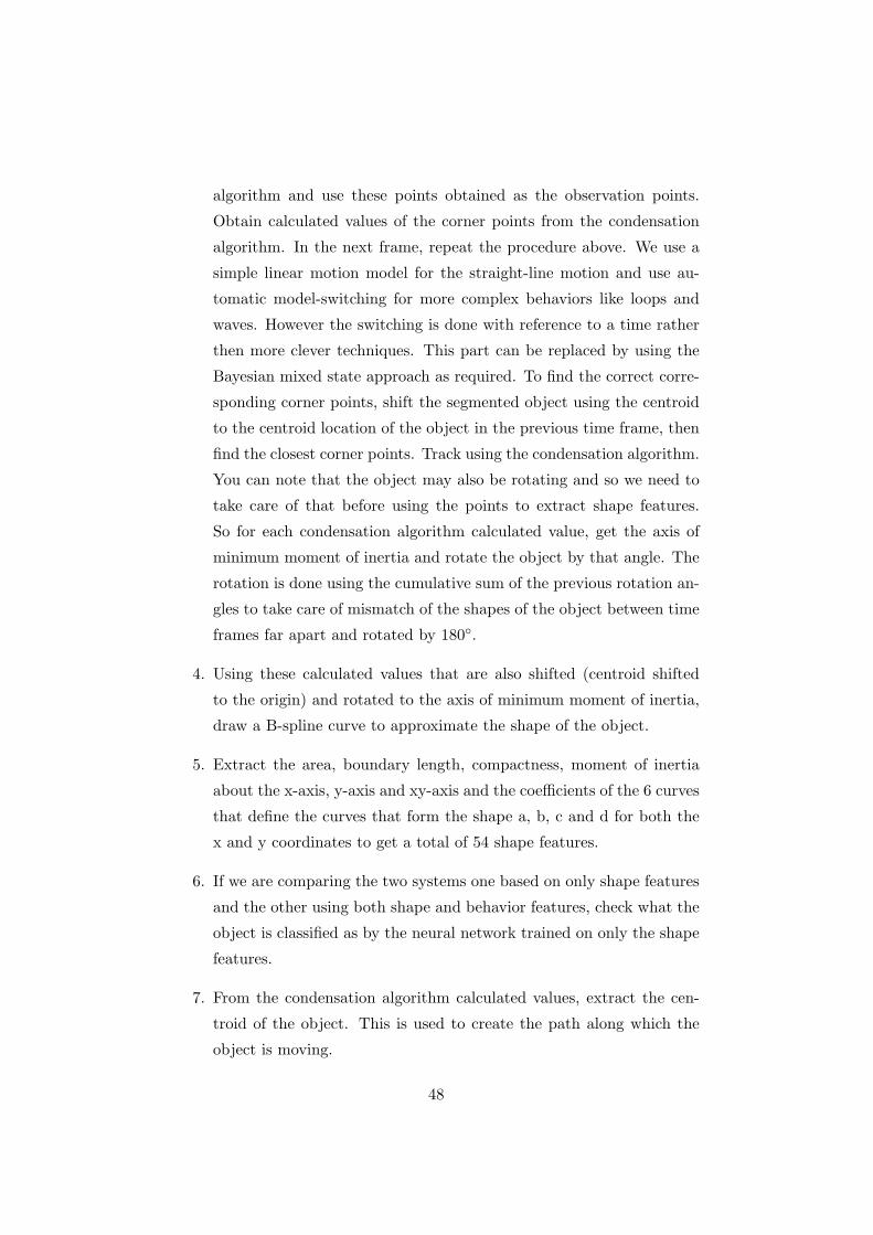
Type 1 - Regular hexagon with a size of 1.0 units.

Type 2 - Regular hexagon with a size of 1.2 units.

Type 3 - Irregular hexagon with the longer side with a size of 1.5 units.

Type 4 - Starship like shape.

Type 5 - Starship like shape with a different angle.

Type 6 - Starship like shape with yet another different angle.

Type 7 - Three pointed star with an inner triangle side of length 0.5 units.

50

Type 8 - Three pointed star with an inner triangle side of length 1 units.

Type 9 - Regular hexagon with a size of 1.1 units

Type 10 - Regular hexagon with a size of 1.05 units

Type 11 - Regular hexagon with a size of 1.01 units

Type 12 - Three pointed star with an inner triangle side of length 0.75

units.

Type 13 - Three pointed star with an inner triangle side of length 0.6 units.

Type 14 - Three pointed star with an inner triangle side of length 0.7 units.

Type 15 - Regular hexagon with a size of 1.02 units

Type 16 - Regular hexagon with a size of 1.03 units

Type 17 - Regular hexagon with a size of 1.04 units

Type 18 - Regular hexagon with a size of 1.005 units

Type 19 - Regular hexagon with a size of 1.015 units

Type 20 - Irregular hexagon with the longer side with a size of 1.49 units

Type 21 - It is an irregular hexagon with the longer side with a size of

1.495 units

Type 22 - Three pointed star with an inner triangle side of length 0.71

units.

Type 23 - Three pointed star with an inner triangle side of length 0.72

units.

Type 24 - Three pointed star with an inner triangle side of length 0.73

units.

Type 25 - Three pointed star with an inner triangle side of length 0.74

units.

51

Figure 5.1: This figure shows a few of the objects used in our study. The

number indicates the object type discussed in the text.

The objects also have behavioral patterns associated with them. Inspired by

the bird flight behavioral dataset illustrated in Fig. 1.1, we create a set of

different paths with can be associated with the object during system testing.

This allows for a larger variety of object shape and behavior combinations.

The object paths also have being designated type numbers. Each is made

up of 5 behavioral features. For most of the them, the start and end features

are straight lines. This helps us be sure of the features that are extracted.

Some of the paths generated and/or tracked are shown in Figs. 6.4 - 6.8.

The object path descriptions include:

Type 1 - straight line, right loop, right loop, right loop, straight line.

Type 2 - straight line, right loop, wave, left loop, straight line.

Type 3 - straight line, left loop, left loop, left loop, straight line.

Type 4 - straight line, wave, left loop, wave, straight line.

Type 5 - straight line, right loop, left loop, right loop, straight line.

Type 6 - straight line, right loop, wave, left loop, straight line.

Type 7 - straight line, left loop, left loop, right loop, straight line.

Type 8 - straight line, left loop, wave, left loop, straight line.

Type 9 - straight line, wave, straight line, wave, straight line.

52

Type 10 - straight line, wave, straight line, right turn, straight line.

Type 11 - straight line, back turn, straight line, wave, straight line.

Type 12 - straight line, left loop, straight line, left turn, straight line.

In each case, a recursive generative model for the ideal trajectory is used,

and Gaussian white noise added at each step. Thus, as can be seen in Fig.

6.4, a straight line segment of the trajectory tends to drift from its original

bearing, actually describing a random walk around its noise-free bearing.

This models the influence random wind gusts might have on a bird’s flight

line when it is intent on flying straight.

5.2 Grammar rules

We define the grammatical rules for extracting the behavioral features.

Small letters stand for terminal symbols and include d for long distance

straight line, s for short distance straight line, b for back turn, l for left turn

, r for right turn, p for hovering effect and e stands for a null. Capital letters

stand for non-terminals and include C for Path, B stands for a back turn, L

for left turn, R for right turn, P for hovering effect, W for wave, T for right

or left loop. D, E, F, G, H, K and J are other intermediate non terminals.

The rules can be given as follows

C → d | H | e

H → KdLdRdK | KdRdLdK | K

K → JdLdJ | JdRdJ | JdLs | sLdJ | JdRs | sRdJ | sLs | sRs | e

J → JdJ | D | e

D → DTD | DWD | E | e

E → EBE | F | e

F → FLF | FRF | G | e

G → s | e

53

B → ll | lsl | lpl | rr | rsr | rpr

L → l

R → r

T → l{s,p}l{s,p}l{s,p}l | r{s,p}r{s,p}r{s,p}r

W → Wl{s,p}r{s,p}l{s,p}r{s,p}l{s,p}r{s,p} |Wr{s,p}l{s,p}r{s,p}l{s,p}r{s,p}l{s,p} | e

5.3 ORMOT

ORMOT is a simulation environment created for demonstration purposes

and for creating test data that may consist of image frames or a video. The

3 screens of this system are shown in Fig. 5.2, 5.3 and 5.4. We can have

many objects moving in the screen as shown in the 3rd screen. ORMOT

provides options including whether you want to create a video file, what

are the screen dimensions you prefer for the path of the objects that will

be simulated, the noise parameters associated with the object, the choice of

objects and the different paths, start positions of the objects, for how much

time you want the objects to move and color of the objects. It also has

options of saving commonly used configurations for faster use later.

5.4 Test data generation

We explain the test data generation as depicted in Fig. 5.5 as follows:

1. We need to select the objects we would like in our setting. Each object

will have its own shape. And each object will have some behavioral

pattern of movement. Select the amount of noise variation you would

like to have as the object moves. For e.g. to take into account the

wind blowing when a bird is flying can be considered as noise. Select

the noise variation in capturing or observing the object. Select the

noise variation in the shape of the object that can be caused by the

segmentation of the object.

54

Figure 5.2: This is the screenshot of the first screen of ORMOT that was cre-

ated for demonstrating the path movement and shape changes of the objects

and creating images which can be used for tracking. Different parameters

cane be set and different paths and object types can be loaded.

55

Figure 5.3: This is the screenshot of the 2nd screen of ORMOT. The objects

can be selected and a path associated with them.

56

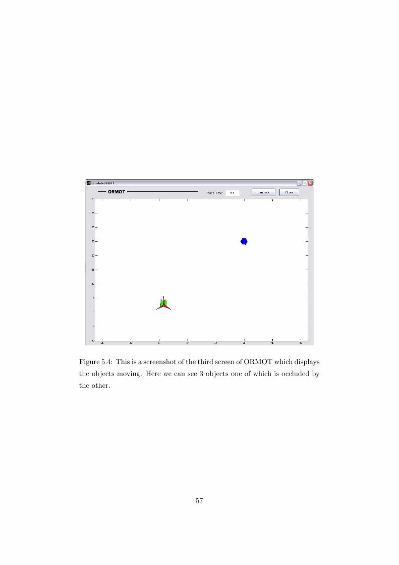
Figure 5.4: This is a screenshot of the third screen of ORMOT which displays

the objects moving. Here we can see 3 objects one of which is occluded by

the other.

57

Figure 5.5: This figure shows how test and training data is generated.

2. Generate the location of the start point of the object randomly. Also

randomly generate the initial velocity and acceleration of the object.

We set the initial speed to be a constant so as to manage to get the

objects entire behavioral pattern in one screen. Note that the initial

directions of movement are random.

3. Generate the path of the object using the equations of motions and

noise variations selected.

4. For each point on the path, generate the corner points of the object

which are variable due to the shape noise added. Note that the centroid

of the object is along the point of path selected.

5. We can capture the entire motion of the objects as a sequence of images

or as a single video.

5.5 Parameters

Some of the important parameters are noted here. These parameters may

have to be changed depending on the domain of the training data that is

used or for faster processing or more accurate tracking.

1. Shape noise standard deviation is the amount of noise you want

in the shape of the object. This parameter can be adjusted so as to

take into account non-rigid body motions or the degree of clutter in

the simulated environment. It also sets the noise during rotation of

the objects. We vary it between 0.05 to 0.25 for different studies.

2. True path noise standard deviation is the amount of noise we

would like to add to a perfect motion system. In reality every motion

of the object is affected by the environment when it is moving may it be

58

friction or air resistance or even the malfunctioning body of the object

for e.g. when a bird is hurt or is not able to flap its wings properly,

the motion of the bird will be affected. These types of disturbances

can be modeled by this parameter. We vary it between 0.05 to 0.1 for

different studies.

3. Observation noise standard deviation is the parameter to take

into account the noise of the instrument or camera capturing the im-

ages as well as the segmentation algorithms. Since we do not actually

perform the segmentation on images, we use this parameter to take

into account the errors that may have been caused by it. We vary it

between 0.025 to 0.075 in our studies.

4. Number of corner points in the object is currently set to 6. We can

set the number of corner points to a variable value with a few changes

to the existing system and by normalizing the averaged shape of the

object.

5. Number of particles in the condensation algorithm can be changed.

Increasing the number of particles may possibly increase the accuracy

of the system up to a limit but the computational complexity of the

algorithm is linear in the number of particles. We used 100 particles

in our study.

6. Lengths and Angles used in the grammar rules for extracting the

behavioral features. The length for a long straight line is defined to

have a threshold of 10 units. A left is defined to have a threshold

angle of +75◦ but not greater than +135◦. A right is defined to have

a threshold angle of −75◦ but not less than −135◦. A back turn is

defined to have an angle turn less than −135◦ or greater than +135◦.

The decision of a turn is based on the cumulative angle for the last

five sample points extracted from the path. Every tenth point in the

B-spline curve corresponding to the smoothed path is chosen as the

sample point for determining the length and angles.

7. Eta is the learning rate of the neural network. It was set to about

0.001 for most of the studies after observation of the fact that for our

59

data having a smaller value drastically reduced the speed by increase

in the number of iterations for no benefit of increase in accuracy.

8. Hidden neurons of the multilayer neural network was set to 5 after

observation that 3 under-represented the data and 7 had no improve-

ment in the accuracy of the system.

9. Number of voters was set to 10.

5.6 Test cases

The goal in choosing the test cases was to show under which circumstances

the addition of behavioral features would improve the accuracy of the object

recognition and under which the additional features would act mainly as

noise instead. With this in mind, 9 test groups were made. Each of these

groups had variations in the noise parameters.

The first test group includes the case where there are 6 objects, all

regular hexagons with slightly different sizes (a difference ratio of 0.01) but

have significantly different behavior patterns. The second has these objects

moving with exactly the same behavior pattern. The third and fourth are

similar to the above respectively except that there are 5 objects and that

the difference in sizes is even less (a difference ratio of 0.005), making the

objects extremely difficult to classify accurately just using shape cues. The

fifth has 4 objects that have shapes like stars and a difference of size of

0.01 and moving with different patterns while the sixth has the 4 objects

moving in the same behavioral pattern. The seventh test group consists of

3 objects that are different in shape and have different behaviors. The eight

has 7 objects that have completely different shapes and different movement

patterns while the ninth has the 7 objects moving in the same behavioral

pattern.

The type number of the object and path of these test cases is shown in

the Tables in the following chapter. Other details such as the size of training

data and test data are also provided.

60

Chapter 6

Results

The following figures show us a few of the results obtained by generating

paths considering noise, tracking of the objects using the condensation al-

gorithm and the extraction of the shapes from the tracked object.

These are the definitions of the acronyms used in the tables that follow.

Iter Maximum iterations training data was trained up to an accuracy of

96% or 20000 iterations whichever is minimum.

SNS Shape Noise Sigma value

TNS True Noise Sigma value

ONS Observed Noise Sigma value

SErr Shape System misclassification

SA % Shape System accuracy percentage

BErr Behavioral System misclassification

BA % Behavioral System accuracy percentage

eta learning rate of the neural network

HN number of hidden neurons

61

Figure 6.1: This figure contains 4 objects that show the object corner points

as observed and as tracked with the help of the condensation algorithm. The

shape noise sigma value was 0.1. (a), (b), (c) and (d) are the objects of type

1, 3, 5 and 7 respectively.

62

Figure 6.2: This figure contains 4 objects that show the object corner points

as observed and as tracked with the help of the condensation algorithm. The

shape noise sigma value was 0.1. (a), (b), (c) and (d) are the objects of type

1, 3, 5 and 7 respectively.

Figure 6.3: This figure consists of 2 sub figures. Each figure has the averaged,

B-spline smoothed shape of the object and centroid shifted to the origin. (a)

is for object of type 1 and (b) is for the object of type 5.

63

Figure 6.4: This is the path of type 2 which consists of a straight line, a

wave, a loop , a wave and a straight line again. The true path is obtained by

corrupting ideal values by a noise sigma of 0.075 and the observed values are

obtained by corrupting the true path by a noise sigma of 0.05. The observed

points are fed to the tracking system.

64

Figure 6.5: This figure of Path type 1 consists of a straight line motion, 3

loops and a straight line motion again. The noise added to the path while

creation of the path had a sigma value of 0.075 while the observation noise

sigma was 0.05. (a) is the entire path while (b) and (c) are the magnified

versions of part of it.

65

Figure 6.6: This is the path of type 11 that consists of a straight line, a back

turn, a straight line, a wave motion and a straight line again. (a) shows the

observed values that are fed to the tracker along with the tracked path and

(b) shows the path smoothed using B-splines from the output of the tracker

system. The blue star points are those sample points used for extracting

the behavioral features.

66

Figure 6.7: This is the path of type 2 which consists of a straight line, a

loop, a wave motion, a loop and a straight line motion again. This is the

smoothed path obtained after applying the B-spline curves to the output of

the path tracked by the condensation algorithm. The blue star points are

chosen as samples of the entire path to extract the behavioral features.

67

Figure 6.8: This is the path of type 10 which consists of a straight line, a

wave motion, a straight line, a right turn and a straight line motion again.

This is the smoothed path obtained after applying the B-spline curves to the

output of the path tracked by the condensation algorithm. The blue star

points are chosen as samples of the entire path to extract the behavioral

features.

68

Table 6.1: Objects type 1, 11, 15, 16, 17, 10 and their path types 1, 2, 3,

4, 5, 6 respectively. The objects are hexagons with size of difference of .01

units and have different behaviors. The training data size was 420 and test

data size was 180.Sr. Iter SNS HN eta SA % BA %

1 4000 0.1 5 0.001 93.889 97.778

2 4000 0.1 5 0.001 92.778 98.333

3 4000 0.1 5 0.001 93.889 98.333

4 10000 0.1 3 0.001 - 98.333

5 10000 0.1 3 0.001 78.333 98.889

6 4000 0.1 7 0.001 93.333 100

7 20000 0.1 7 0.0001 93.333 98.333

8 10000 0.2 5 0.001 76.111 95

9 20000 0.2 3 0.001 73.889 95.556

10 20000 0.2 7 0.001 74.444 93.333

Table 6.2: Objects type 1, 11, 15, 16, 17, 10 and their path types 1, 2, 3,

4, 5, 6 respectively. The objects are hexagons with size of difference of .01

units and have different behaviors. The training data size was 420 and test

data size was 180.Sr. Iter SNS TNS ONS SErr SA % BErr BA %

1 420 0.1 0.075 0.05 11 93.89 1 99.44

2 1658 0.2 0.075 0.05 43 76.11 6 96.67

3 660 0.15 0.075 0.05 33 81.67 6 96.67

4 10000 0.25 0.075 0.05 65 63.89 14 92.22

5 1887 0.05 0.075 0.05 0 100.00 1 99.44

6 197 0.1 0.05 0.025 12 93.33 3 98.33

7 244 0.1 0.02 0.02 7 96.11 1 99.44

8 1021 0.1 0.1 0.075 16 91.11 9 95.00

69

Table 6.3: Objects type 1, 11, 15, 16, 17, 10 and their path types 2, 2, 2,

2, 2, 2 respectively. The objects are hexagons with size of difference of .01

units and have same behaviors. The training data size was 420 and test

data size was 180.Sr. Iter SNS TNS ONS SErr SA % BErr BA %

1 1876 0.1 0.075 0.05 7 96.11 9 95.00

2 10000 0.2 0.075 0.05 47 73.89 54 70.00

3 4633 0.15 0.075 0.05 30 83.33 35 80.56

4 10000 0.25 0.075 0.05 59 67.22 68 62.22

5 3230 0.05 0.075 0.05 1 99.44 0 100.00

6 789 0.1 0.05 0.025 11 93.89 16 91.11

7 10000 0.1 0.2 0.2 14 92.22 13 92.78

8 1703 0.1 0.1 0.075 11 93.89 12 93.33

Table 6.4: Objects type 1, 18, 11, 19, 15 and their path types 1, 2, 3, 4, 5

respectively. The objects are hexagons with size of difference of .005 units

and have different behaviors. The training data size was 350 and test data

size was 150.Sr. Iter SNS TNS ONS SErr SA % BErr BA %

1 526 0.1 0.075 0.05 30 80.00 1 99.33

2 1547 0.2 0.075 0.05 79 47.33 12 92.00

3 536 0.15 0.075 0.05 50 66.67 8 94.67

4 10000 0.25 0.075 0.05 84 44.00 22 85.33

5 409 0.05 0.075 0.05 14 90.67 1 99.33

6 389 0.1 0.05 0.025 28 81.33 2 98.67

7 217 0.1 0.2 0.2 36 76.00 2 98.67

8 3935 0.1 0.1 0.075 38 74.67 15 90.00

70

Table 6.5: Objects type 1, 18, 11, 19, 15 and their path types 2, 2, 2, 2, 2, 2

respectively. The objects are hexagons with size of difference of .005 units

and have the same behaviors. The training data size was 350 and test data

size was 150.Sr. Iter SNS TNS ONS SErr SA % BErr BA %

1 20000 0.1 0.075 0.05 36 76.00 38 74.67

2 20000 0.2 0.075 0.05 78 48.00 71 52.67

3 20000 0.15 0.075 0.05 49 67.33 55 63.33

4 20000 0.25 0.075 0.05 79 47.33 79 47.33

5 2212 0.05 0.075 0.05 8 94.67 4 97.33

6 20000 0.1 0.05 0.025 32 78.67 35 76.67

7 20000 0.1 0.2 0.2 35 76.67 35 76.67

8 20000 0.1 0.1 0.075 33 78.00 39 74.00

Table 6.6: Objects type 22, 23, 24, 25 and their path types 5, 6, 7, 8

respectively. The objects are star shapes with a size difference of .01 units

and have different behaviors. The training data size was 280 and test data

size was 120.Sr. Iter SNS TNS ONS SErr SA % BErr BA %

1 673 0.1 0.075 0.05 43 64.17 2 98.33

2 6448 0.2 0.075 0.05 65 45.83 17 85.83

3 5769 0.15 0.075 0.05 60 50.00 11 90.83

4 20000 0.25 0.075 0.05 73 39.17 32 73.33

5 401 0.05 0.075 0.05 17 85.83 1 99.17

6 340 0.1 0.05 0.025 45 62.50 6 95.00

7 444 0.1 0.2 0.2 42 65.00 2 98.33

8 20000 0.1 0.1 0.075 43 64.17 14 88.33

71

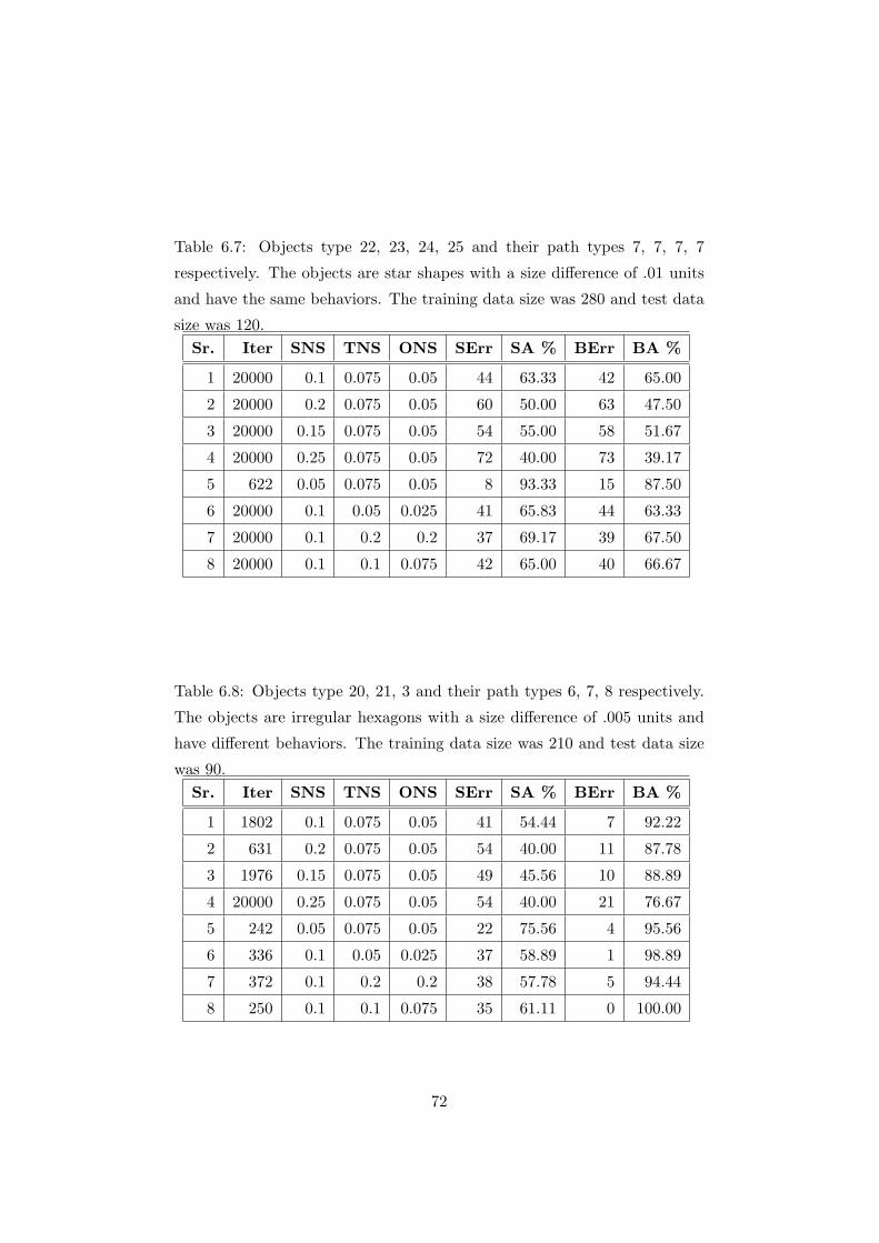
Table 6.7: Objects type 22, 23, 24, 25 and their path types 7, 7, 7, 7

respectively. The objects are star shapes with a size difference of .01 units

and have the same behaviors. The training data size was 280 and test data

size was 120.Sr. Iter SNS TNS ONS SErr SA % BErr BA %

1 20000 0.1 0.075 0.05 44 63.33 42 65.00

2 20000 0.2 0.075 0.05 60 50.00 63 47.50

3 20000 0.15 0.075 0.05 54 55.00 58 51.67

4 20000 0.25 0.075 0.05 72 40.00 73 39.17

5 622 0.05 0.075 0.05 8 93.33 15 87.50

6 20000 0.1 0.05 0.025 41 65.83 44 63.33

7 20000 0.1 0.2 0.2 37 69.17 39 67.50

8 20000 0.1 0.1 0.075 42 65.00 40 66.67

Table 6.8: Objects type 20, 21, 3 and their path types 6, 7, 8 respectively.

The objects are irregular hexagons with a size difference of .005 units and

have different behaviors. The training data size was 210 and test data size

was 90.Sr. Iter SNS TNS ONS SErr SA % BErr BA %

1 1802 0.1 0.075 0.05 41 54.44 7 92.22

2 631 0.2 0.075 0.05 54 40.00 11 87.78

3 1976 0.15 0.075 0.05 49 45.56 10 88.89

4 20000 0.25 0.075 0.05 54 40.00 21 76.67

5 242 0.05 0.075 0.05 22 75.56 4 95.56

6 336 0.1 0.05 0.025 37 58.89 1 98.89

7 372 0.1 0.2 0.2 38 57.78 5 94.44

8 250 0.1 0.1 0.075 35 61.11 0 100.00

72

Table 6.9: Objects type 1, 4, 6, 9, 12, 20, 22 and their path types 2, 3, 4, 5,

6, 7, 8 respectively. The objects have totally different shapes and behaviors.

The training data size was 245 and test data size was 105.

Sr. Iter SNS TNS ONS SErr SA % BErr BA %

1 308 0.1 0.075 0.05 0 100.00 0 100.00

2 501 0.2 0.075 0.05 0 100.00 0 100.00

3 7727 0.15 0.075 0.05 0 100.00 1 99.05

4 384 0.25 0.075 0.05 0 100.00 1 99.05

5 6405 0.05 0.075 0.05 0 100.00 1 99.05

6 230 0.1 0.05 0.025 0 100.00 1 99.05

7 179 0.1 0.2 0.2 1 99.05 1 99.05

8 742 0.1 0.1 0.075 1 99.05 2 98.10

Table 6.10: Objects type 1, 4, 6, 9, 12, 20, 22 and their path types 4, 4, 4, 4,

4, 4, 4 respectively. The objects have totally different shapes but have the

same behavior. The training data size was 245 and test data size was 105.

Sr. Iter SNS TNS ONS SErr SA % BErr BA %

1 1003 0.1 0.075 0.05 0 100.00 0 100.00

2 20000 0.2 0.075 0.05 0 100.00 0 100.00

3 4076 0.15 0.075 0.05 0 100.00 2 98.10

4 337 0.25 0.075 0.05 0 100.00 0 100.00

5 625 0.05 0.075 0.05 0 100.00 0 100.00

6 1337 0.1 0.05 0.025 0 100.00 0 100.00

7 1476 0.1 0.2 0.2 0 100.00 0 100.00

8 310 0.1 0.1 0.075 0 100.00 1 99.05

73

Chapter 7

Conclusions and Future work

7.1 Conclusions

The goal of this study was to discover if the use of the dynamic content of

image sequences coded as behavioral features can aid in object recognition.

From the results obtained and shown in the previous chapter we draw the

following conclusions:

1. If we are able to define and retrieve the behavioral features reasonably

well, and if the characteristic behaviors of similarly appearing object

classes are reasonably distinct, then they provide a source of valuable

information for object recognition systems.

2. We have favored shape in the above study by choosing objects that are

quasi-rigid, i.e. don’t change their shape greatly over the entire image

sequence. Shape changes are limited to small amounts of noise added

to the shape models over time. If the shapes of objects occupying dis-

tinct object classes are pretty similar, then a learning system that uses

only shape features does not do a very good job. In our experiments,

the error rate in such cases was up to 30%. In such cases augment-

ing the system with behavioral features is more robust against shape

changes and exhibits an improved error rate of 5% on an average for

our experiments.

3. If we train a system with objects that have very similar shapes as well

74

as behavioral patterns, then the system which uses both shape and

behavior cues may perform worse that the shape-only system. This

is likely due to the fact that the behavior features have relatively low

information content, with most of their variation due to noise. Thus

the added noisy features decrease overall signal to noise ratios and

thus performance.

4. The same conclusion can be made about the objects that are reliably

and clearly dissimilar in shape and move as rigid bodies with similar

behaviors. In this case shape information is sufficient for accurate class

recognition. Behavioral information, being of lower quality than shape

information, can confuse an otherwise accurate system.

In sum, we conclude that for a range of dynamic object recognition

problems, recognition systems cued by both shape and behavioral features

are both more accurate and robust. One such class of problems are those

in which object shapes are similar or shape is observed with significant

random noise or distortion. In circumstances where shapes are quite distinct

and clearly observed, behavioral cues are not likely to improve performance

noticeably, and may in fact degrade system performance.

7.2 Future work

Quite a lot of work can be done in extending the current system. We consid-

ered objects that were quasi-rigid and did not change shape radically over

time. Variability of shape is prone to degrade a system that relies only on

shape features. If such objects have some patterns of movement, they can

be used in a combined shape-behavior system for an improved performance.

Also, we did not model rotational motion of objects in this proof-of-concept

design. Canonical reorientation of objects would result in some noise. This

may be simulated to check the effect on the shape and behavioral system.

We have not implemented the corner point detection of the objects. We

do try to include noise in the system to take care of these effects though.

The paths currently are of a standard size so as to be able to be captured

in a screen size. Normalization of the paths can be done in future ver-

75

sions. We may use a hybrid model consisting of a dynamic time warping

algorithm, hidden Markov model and a neural network for learning of the

behavioral features. We have restricted the number of behavioral features

fixed at 5 for the tests done. We can make that variable to accommodate

different behavior properties of different objects. Concerning the nature of

behavioral features, we can use speed, radius of curvature in turns, and

regional loitering time as other behavioral features for a normalized input

image sequence. The system can be made smarter by checking to see how

the shape-behavioral system does compared to the shape system alone. If

the shape system performs better on the validation data we need to use

the shape system results else we can rely on the results of the shape and

behavioral system.

Finally, the use of behavioral features at more primitive levels, those

considered as pre-processing levels in the present study, can be combined

with its use as above to explore the full use of behavior in dynamic visual

object recognition. In a related study [34] has considered the use of behavior

to enhance dynamic segmentation. We propose to collaborate to see the

degree to which behavior, exploited both in the early image processing and

in the late computer vision stages, impacts the quality of dynamic visual

object recognition.

76

Bibliography

[1] C. BenAbdelkader, R. Cutler, and L. Davis, “Stride and cadence as

a biometric in automatic person identification and verification,” Au-

tomatic face and Gesture Recognition, 2002, Fifth IEEE proceedings ,

pp. 357–362, 2002.

[2] W. Hu, T. Tan, L. Wang, and S. Maybank, “A survey on visual surveil-

lance of object motion and behaviors,” Systems, Man and Cybernetics,

IEEE Transactions on 34(3), pp. 334–352, 2004.

[3] I. Haritaoglu, D. Harwood, and L. S. Davis, “W4: real-time surveil-

lance of people and their activities,” Pattern Analysis and Machine

Intelligence, IEEE Transactions on 22(8), pp. 809–830, 2000.

[4] A. Diplaros, T. Gevers, and I. Patras, “Combining color and shape in-

formation for illumination-viewpoint invariant object recognition,” Im-

age Processing, IEEE Transactions on 15(1), pp. 1–11, 2006.

[5] M. Hahnel, D. Klunder, and K. Kraiss, “Color and texture features for

person recognition,” Neural Networks, 2004. Proceedings. 2004 IEEE

1, p. 652, 2004.

[6] G. Ji, G. Wang, Z. Houkes, B. Zheng, and Y. Han, “A new method for

fast computation of moments based on 8-neighbor chain code applied

to 2-d object recognition,” Intelligent Processing Systems, 1997. ICIPS

’97. 1997 IEEE International Conference 2, p. 974, 1997.

[7] M. Y. Mashor, M. K. Osman, and M. R. Arshad, “3d object recognition

using 2d moments and hmlp network,” Computer Graphics, Imaging

and Visualization, 2004. CGIV 2004. Proceedings , p. 126, 2004.

77

[8] P. L. Worthington and E. R. Hancock, “Object recognition using

shape-from-shading,” Pattern Analysis and Machine Intelligence, IEEE

Transactions on 23(5), pp. 535–542, 2001.

[9] S. Belongie, J. Malik, and J. Puzicha, “Shape matching and object

recognition using shape contexts,” Pattern Analysis and Machine In-

telligence, IEEE Transactions on 24(4), pp. 509–522, 2002.

[10] E. Bala and A. E. Cetin, “Computationally efficient wavelet affine in-

variant functions for shape recognition,” Pattern Analysis and Machine

Intelligence, IEEE Transactions on 26(8), pp. 1095–1099, 2004.

[11] C. M. Cyr and B. B. Kimia, “3D object recognition using shape

similiarity-based aspect graph,” Computer Vision, 2001. ICCV 2001.

Proceedings. Eighth IEEE International Conference on 1, pp. 254–261,

2001.

[12] C. Liu and N. Ahuja, “A model for dynamic shape and its applica-

tions,” Computer Vision and Pattern Recognition, 2004. CVPR 2004.

Proceedings of the 2004 IEEE 2, p. 129, 2001.

[13] S. Pansang and C. Kimpan, “3-D object recognition from shadow shape

curves,” Circuits and Systems, 2000. IEEE APCCAS 2000 , pp. 437–

440, 2000.

[14] B. Neumann, “Simple 2D shape features,” kogs-www.informatik.uni-

hamburg.de/ neumann/BV-SS-2002/BV-L8.pdf .

[15] R. H. Bartels, J. C. Beatty, and B. A. Barsky, An Introduction to Splines

for Use in Computer Graphics and Geometric Modeling, Morgan Kauf-

mann Publishers, Inc., 1987.

[16] Wikipedia, “Behavior,” http://en.wikipedia.org/wiki/Behavior .

[17] A. Feldmann and T. Balch, “Representing honey bee behavior for recog-

nition using human trainable models,” Adaptive Behavior , 2004.

[18] A. Kale, A. N. Rajagopalan, N. Cuntoor, and V. Kruger, “Gait-based

recognition of humans using continuous hmms,” Automatic face and

Gesture Recognition, 2002, Fifth IEEE proceedings , pp. 321–326, 2002.

78

[19] R. Cutler and L. S. Davis, “Robust real-time periodic motion detection,

analysis and applications,” Pattern Analysis and Machine Intelligence,

IEEE Transactions on 22(8), pp. 781–796, 2000.

[20] C. Lu and N. J. Ferrier, “Repetitive motion analysis: segmentation and

event classification,” Pattern Analysis and Machine Intelligence, IEEE

Transactions on 26(2), pp. 258–263, 2004.

[21] E. B. Koller-Meier and L. V. Gool, “Modeling and recognition of human

actions using a stochastic approach,” citeseer.ist.psu.edu/499804.html .

[22] N. Johnson and D. Hogg, “Learning the distribution of object trajecto-

ries for event recognition,” Image and Vision computing, Science Direct

, 1999.

[23] A. Galata, N. Johnson, and D. Hogg, “Learning variable-length markov

models of behavior,” Computer Vision and Image Understanding , 2002.

[24] J. Chamorro-Martinez, J. Fdez-Valdividia, J. A. Garcia, and

J. Martinez-Baena, “A frequency-domain approach for the extraction of

motion patterns,” Acoustics, Speech and Signal Processing, 2003, IEEE

Proceedings 3, p. 165, 2003.

[25] A. J. Lipton, H. Fujiyoshi, and R. S. Patil, “Moving target classifica-

tion and tracking from real-time video,” Automatic face and Gesture

Recognition, 2002, Fifth IEEE proceedings , pp. 357–362, 2002.

[26] P. S. Maybeck, Stochastic models, estimation, and control (Volume 1).

[27] Z. Chen, “Bayesian filtering: From kalman filters to particle filters and

beyond.”.

[28] N. J. Gordon, D. J. Salmond, and A. F. M. Smith, “Novel approach to

nonlinear/non-gaussian bayesian state estimation,” Radar and Signal

Processing, IEEE Proceedings 140(2), pp. 107–113, 1993.

[29] M. Isard and A. Blake, “Condensation - conditional density propagation

for visual tracking,” Int. Journal of Computer Vision 29(1), pp. 5–28,

1998.

79

[30] J. E. Hopcroft and J. D. Ullman, Introduction to Automata Theory,

Languages and Computation, Addison-Wesley Publications, 1979.

[31] T. M. Mitchell, Machine Learning, McGraw-Hill International Editions,

1997.

[32] Wikipedia, “Multilayer neural network,”

http://upload.wikimedia.org/wikipedia/en/4/43/Neural Network.gif .

[33] C. Harris and M. Stephens, “A combined corner and edge detector,”

Fourth Alvey Vision Conference , pp. 147–151, 1998.

[34] R. Krishna, “A framework for unifying shape and behavior models for

motion segmentation.” Report at SUNY-University at Buffalo.

80