Object-Oriented Dynamic Bayesian Network-Templates for Modelling Mechatronic Systems

Harald Renninger and Hermann von Hasseln

DaimlerChrysler AG Research and Technology (REM/E)D-70546 Stuttgart, Germany

{harald.renninger, hermann.v.hasseln}@daimlerchrysler.com

Abstract

The object-oriented paradigma is a new but proven technol-ogy for modelling mechatronics, i.e. multidisciplinary mod-elling. For many reasons the object-oriented approach isvery much desirable also for qualitative models in systemdesign, diagnosis or verification. Bayesian networks are avery robust technology for qualitative probabilistic model-ling. In this paper we present a first approach in using theBayesian networks modelling technique with the quantita-tive object-oriented method. Analogous to Modelica, anobject-oriented modelling language, we constructed a Baye-sian network library for modelling hydraulic systems. TheseBayesian networks are called Object Oriented DynamicBayes Nets (OODBNs). Our method is easily transferable toany other physical domain or logic. In this contribution ourmotivation and the construction steps are described. Simula-tion results for a sample hydraulic system are given.

Introduction

Future system architectures will be characterized byhighly modular and reusable components, and by abstractdescription languages widely independent of implementa-tion details. Typical components of system architectures aresoftware and hardware (sub-)systems. On the Software sidethe object-oriented paradigma is by now (at least in indus-trial applications) the de facto description or modelling lan-guage standard, mostly represented by the UnifiedModelling Language (UML). On the Hardware side, whichis our focus here, we have mechatronic hardware compo-nents, the constituent parts of which are control logics andcontrolled physical or chemical systems. Modelling mecha-tronic systems challenges the engineer due to differentphysical domains. In order to reach the goal of a truly uni-fied description of system architectures comprising Soft-ware and Hardware systems, the description or modellinglanguages of mechatronic systems have to be lifted to asimilar abstract level as their Software counterparts.

Model based techniques play an important role in con-current and future engineering processes. Models and simu-lations are a basis for system design and analysis, e.g. forgeometric layout of hydraulic systems. On the other hand,model based control and model based diagnosis are state ofthe art.

Many different philosophies have been developed to sup-port the modelling task. In the control engineering areatools like Matlab/Simulink [1] or MatrixX SystemBuild [2]

are widespread. For modelling mechanical systemsADAMS [3] or SIMPACK [4] are frequently used. Forelectronic systems PSPICE [5] is an appropriate tool. Otherspecific tools are used to solve modelling tasks in flowdynamics, thermal flow or chemical processes. Each ofthese programs are specially tailored for the specificdomain.

A mechatronic system consists of a control logic, elec-tronics and a controlled mechanical, hydraulic or any otherphysical or chemical system. The entire system is com-posed of subsystems of different domains. This shows therestriction of all classical modelling systems, since the con-trol part can be easily described for example in Matlab/Simulink, but it is nearly impossible to model an electricalsubsystem. So, a method is needed for a multidisciplinarymodelling.

Methods and tools, e.g. Omola, Dymola or Smile, havebeen developed which allow multidisciplinary modelling.Modelica [6], [7] is the latest step in this direction. It is astandardized object-oriented modelling language which issupported by the tool Dymola [8] for example.

Dymola/Modelica comes with libraries for differentphysical domains like electrics/electronics, mechanics,thermal flow or hydraulics, see Figure 1. It also contains asignal block and a Petri net library. A library consists of aset of templates for different physical or logical objects.The user can extend a library for example by inheritance orcan create completely new libraries. A model is describedby an object diagramm. Most tools contain a graphicalinterface with a simple drag and drop technique for the tem-plates and interconnections at the object interfaces. Theinterconnections have the meaning of constraints. Moreprecisely, two types of equations are generated when twophysical objects are connected: a flow and a potential equa-tion. With the definition of the flow and the potential vari-ables, the energy flow in the interface is uniquely defined.This is valid for all lumped parameter systems. The greatadvantage is that the system can now be modelled by localbehaviour and not by global analysis [9], which supportsthe general idea of modularity.

Qualitative Models and Bayesian NetworksQualitative modelling offers many well-known advan-

tages for system design, diagnosis or verification, see [14]for a very extensive survey of techniques and applications.Some of these advantages are:

• handling of incomplete and imprecise knowledge,• robustness,• easy comparison of system alternatives, e.g. parameters

variations,• direct interpretation of simulation results,• complexity.

Our vision is an object-oriented method using Bayesian net-works for modelling physical systems, especially systemdynamics. Bayesian networks are a well-suited method forhandling imprecise knowledge in a consistent way. Efficientlearning and adaption algorithms are known for Bayesiannetworks, which is a very interesting option for automaticmodel calibration. The definition of a Bayesian network BNis as follows: BN = {DAG, CPDs}, where DAG is a directedacyclic graph, consisting of nodes and directed edges orlinks, and CPDs are conditional probability distributions.The nodes in a Bayesian network represent propositionalvariables of interest (e.g., the temperature of a device). Thelinks of a BN represent informational or causal dependenciesamong the variables. These dependencies are quantified byconditional probabilties (the CPDs) for each node given itsparental nodes in the DAG. We do not cite the Bayesian net-works fundamentals in this paper, but refer to the relevant lit-erature, see [10] for some Bayesian networks basics or [11]for an excellent textbook.

Object-oriented Bayesian networks were introduced in[13], and are now supported by the newest version of thecommercial Software tool HUGIN [12] for example.

Template constructionIn this section we describe the conversion steps from

Modelica to Bayesian network templates. The conversionwill proceed in four major steps. First, given a dynamic com-ponent, the differential equations will be discretized in timeusing Euler's rule. Second, the equation part of a Modelicatemplate will be reformulated with qualitative operators.Third, the qualitativ landmarks have to be chosen for eachstate variable and each parameter. Fourth, the resulting qual-itative equations will be graphically programmed with Baye-sian networks.

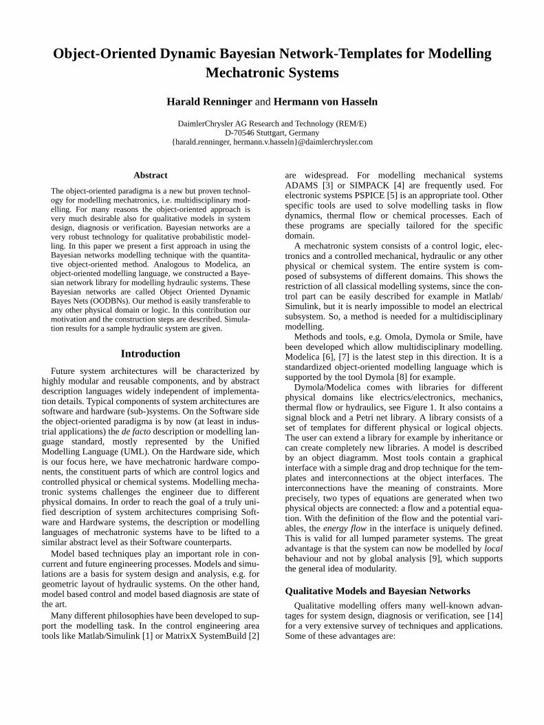
An fuel reservoir called "VolumeConst" will serve as anexample. The icon used in the Modelica HyLib library [15]is shown in Figure 2. Note, that the component VolumeConsthas one port (portA) and that the flow into the componenthas a positive sign . PortA can be viewed as a real physicalflange with some pressure p and an oil flow q. The behaviorof the component VolumeConst is described in Modelica bythe equation block. Other definition blocks like the graphi-cal, interfaces or parameter block are omitted.

Figure 1: The hydraulics library and an object diagram in Dymola.

model VolumeConstgraphical blockinterfaces blockparameter blockequation

end VolumeConst

The equation block consists of one differential equationwith beta and volume being fixed parameters defining theeffective bulk modulus of the liquid and the volume insquare meters, respectively. After chosing a time step h thetime discrete version is as follows:

model VolumeConstDiscrequation

end VolumeConstDiscr

Next, qualitative operators are inserted.

model VolumeConstQualequation

end VolumeConstQual

Now we have to choose a quantity space, the "landmarks",for the variables and parameters. For clearness, we choose athree valued quantity space for all variables .Some qualitative calculus has to be defined for the chosenquantity space. Qualitative addition for the three valuedquantity space can be defined straightforward [14] as inTable 1.

The entry marks the ambiguity of the result, whenthe operator is applied on and or vice versa,respectively.

Now the Bayesian network template for VolumeConst canbe constructed. The basic idea is to identify each qualitativevariable with a Bayesian network node, the qualititative val-ues with the states of this node, and the qualitative calculuswith CPDs.

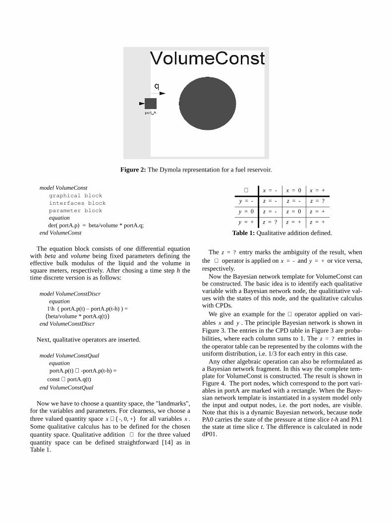
We give an example for the operator applied on vari-ables and . The principle Bayesian network is shown inFigure 3. The entries in the CPD table in Figure 3 are proba-bilities, where each column sums to 1. The entries inthe operator table can be represented by the colomns with theuniform distribution, i.e. 1/3 for each entry in this case.

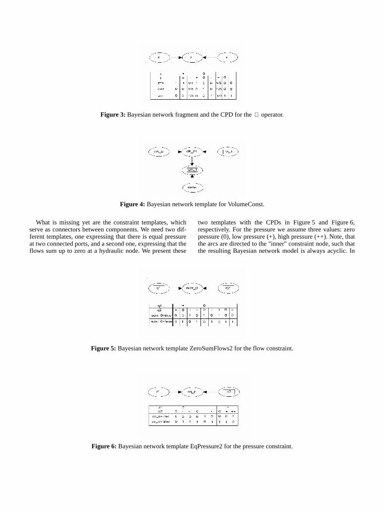
Any other algebraic operation can also be reformulated asa Bayesian network fragment. In this way the complete tem-plate for VolumeConst is constructed. The result is shown inFigure 4. The port nodes, which correspond to the port vari-ables in portA are marked with a rectangle. When the Baye-sian network template is instantiated in a system model onlythe input and output nodes, i.e. the port nodes, are visible.Note that this is a dynamic Bayesian network, because nodePA0 carries the state of the pressure at time slice t-h and PA1the state at time slice t. The difference is calculated in nodedP01.

Figure 2: The Dymola representation for a fuel reservoir.

der( portA.p) beta/volume * portA.q;=

1\h ( portA.p(t) portA.p(t-h) ) =– beta/volume * portA.q(t)( )

portA.p(t) -portA.p(t-h) =⊕const portA.q(t)⊗

x -, 0, +{ }∈ x

⊕

Table 1: Qualitative addition defined.

⊕ x -= x 0= x +=

y -= z -= z -= z ?=

y 0= z -= z 0= z +=

y += z ?= z += z +=

z ?=

⊕ x -= y +=

⊕x y

z ?=

What is missing yet are the constraint templates, whichserve as connectors between components. We need two dif-ferent templates, one expressing that there is equal pressureat two connected ports, and a second one, expressing that theflows sum up to zero at a hydraulic node. We present these

two templates with the CPDs in Figure 5 and Figure 6,respectively. For the pressure we assume three values: zeropressure (0), low pressure (+), high pressure (++). Note, thatthe arcs are directed to the "inner" constraint node, such thatthe resulting Bayesian network model is always acyclic. In

Figure 3: Bayesian network fragment and the CPD for the operator.

Figure 4: Bayesian network template for VolumeConst.

⊕

Figure 5: Bayesian network template ZeroSumFlows2 for the flow constraint.

Figure 6: Bayesian network template EqPressure2 for the pressure constraint.

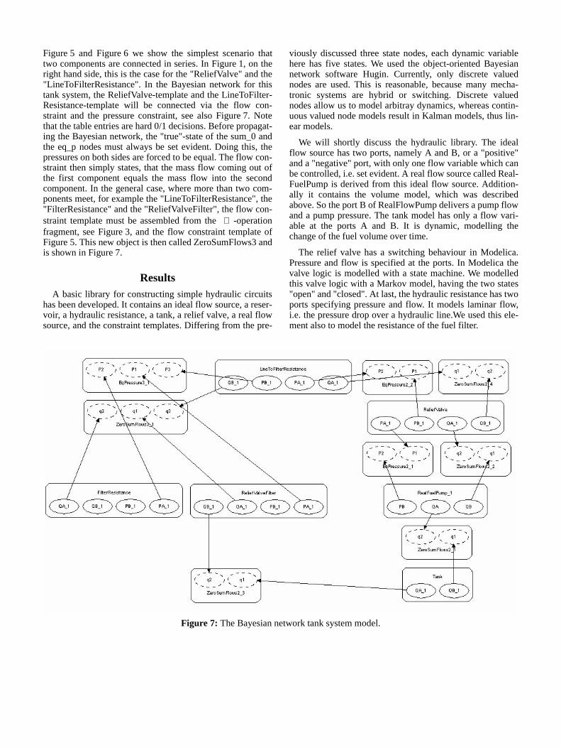
Figure 5 and Figure 6 we show the simplest scenario thattwo components are connected in series. In Figure 1, on theright hand side, this is the case for the "ReliefValve" and the"LineToFilterResistance". In the Bayesian network for thistank system, the ReliefValve-template and the LineToFilter-Resistance-template will be connected via the flow con-straint and the pressure constraint, see also Figure 7. Notethat the table entries are hard 0/1 decisions. Before propagat-ing the Bayesian network, the "true"-state of the sum_0 andthe eq_p nodes must always be set evident. Doing this, thepressures on both sides are forced to be equal. The flow con-straint then simply states, that the mass flow coming out ofthe first component equals the mass flow into the secondcomponent. In the general case, where more than two com-ponents meet, for example the "LineToFilterResistance", the"FilterResistance" and the "ReliefValveFilter", the flow con-straint template must be assembled from the -operationfragment, see Figure 3, and the flow constraint template ofFigure 5. This new object is then called ZeroSumFlows3 andis shown in Figure 7.

ResultsA basic library for constructing simple hydraulic circuits

has been developed. It contains an ideal flow source, a reser-voir, a hydraulic resistance, a tank, a relief valve, a real flowsource, and the constraint templates. Differing from the pre-

viously discussed three state nodes, each dynamic variablehere has five states. We used the object-oriented Bayesiannetwork software Hugin. Currently, only discrete valuednodes are used. This is reasonable, because many mecha-tronic systems are hybrid or switching. Discrete valuednodes allow us to model arbitray dynamics, whereas contin-uous valued node models result in Kalman models, thus lin-ear models.

We will shortly discuss the hydraulic library. The idealflow source has two ports, namely A and B, or a "positive"and a "negative" port, with only one flow variable which canbe controlled, i.e. set evident. A real flow source called Real-FuelPump is derived from this ideal flow source. Addition-ally it contains the volume model, which was describedabove. So the port B of RealFlowPump delivers a pump flowand a pump pressure. The tank model has only a flow vari-able at the ports A and B. It is dynamic, modelling thechange of the fuel volume over time.

The relief valve has a switching behaviour in Modelica.Pressure and flow is specified at the ports. In Modelica thevalve logic is modelled with a state machine. We modelledthis valve logic with a Markov model, having the two states"open" and "closed". At last, the hydraulic resistance has twoports specifying pressure and flow. It models laminar flow,i.e. the pressure drop over a hydraulic line.We used this ele-ment also to model the resistance of the fuel filter.

⊕

Figure 7: The Bayesian network tank system model.

We present a little hydraulic circuit, that is, a fictitioustank system. This system was first modelled for reference inDymola/Modelica, see Figure 1 on the right hand side. Thenwe built this system using the dynamic Bayesian networktemplates. The Bayesian network tank system is shown inFigure 7. For the dynamic simulation, we set evident all con-straint nodes and the pump flow. All other nodes are hidden,

that is, they were calculated by propagation. The results for100 time steps are shown in Figure 8, Figure 9, andFigure 10. These figures show the evolution of the probabil-ity distributions. The darker the colour bars are, the higherthe probability. We added mean values for conveniance. Theplots were produced using the Qualitative Modelling Tool-box for Matlab SIMULINK [16].

Conclusion and future workIn this contribution we have motivated the need for intelli-

gent modelling techniques. For system design, diagnosis orverification qualitative models are a very good choice. Wefavor the Bayesian network technology due to their robust-ness, intuitivity and practicability.

We seeked a qualitative modelling technique for mecha-tronic systems, i.e. for dynamic, multidomain systems. Theobject-oriented physical modelling technique gave us thehint for the construction of our OODBNs. The simulationresults encourage us to proceed in this direction. Recent suc-

cess has been made to select the states (the "landmarks")upon measurements or quantitative simulations, using a sim-ple heuristic from system identification. Furthermore, learn-ing respectively adapting the CPDs using HUGINs adaptionAPI was very promising.

References

[1] SIMULINK. Homepage: http://www.Mathworks.com/

[2] SYSTEMBUILD. Homepage: http://www.isi.com/

Figure 8: The pump flow (evident node).

Figure 9: The flow into the fuel reservoir VolumeConst (inside the RealFuelPump template - hidden node).

Products/MATRIXx/

[3] ADAMS. Homepage: http://www.adams.com/

[4] SIMPACK. Homepage: http://www.simpack.de/

[5] PSPICE. Homepage: http://www.microsim.som/

[6] Elmqvist, H.; Mattsson, S.E.; Otter, M.1999. Modelica - A Language for Physical System Modeling, Visualiza-tion and Interaction. IEEE Symposium on Computer-Aided System Design, CACSD’99, Hawaii, August 22-27, 1999.

[7] Modelica. Homepage http://www.modelica.org

[8] Dymola. Homepage http://www.dynasim.se

[9] Otter, M. et al. 1999. Objektorientierte Modellierung Physikalischer Systeme, Teil 1. at - Automatisierung-stechnik 47, pp.A1-A4. Continued in the following issues of the at.

[10] Jensen, F. 1996. Bayesian networks basics. AISB Quar-terly 94, pp. 9-22.

[11] Cowell, R.G., Dawid, A.P., Lauritzen, S.L., Spiegelhal-ter, D.J. 1999. Probabilistic Networks and Expert Sys-tems. Statistics for Engineering and Information Science. Jordan, Lauritzen, Lawless, Nair (eds.), Springer-Verlag New York Inc. ISBN 0-387-98767-3.

[12] Hugin. Homepage: http://www.hugin.com/

[13] Koller, D., Pfeffer, A. 1997. Object-oriented bayesian networks, Proceedings of the thirteenth conference on Uncertainty in Artificial Intelligence, UAI 97.

[14] Dague, P.et al. 1995. Qualitative Reasoning: A Survey of Techniques and Applications.AICOM Vol. 8, Nrs. 3/4, Sept./Dec. pp. 119--192.

[15] Beater, P. 1998. Object-oriented Modeling and Simula-tion of Hydraulic Drives. Simulation News Europe, SNE 22, pp. 11-13.

[16] G. Lichtenberg et.al. Qualitative Modelling Toolbox User’s Guide. Release 5.2. Download: http://pcweb.rts.tu-harburg.de/inter/homepage.nsf

Figure 10: The ReliefValve behavior (hidden node), where ’0’ means closed, and ’1’ means open.