Object Detection in Multi-modal Images Using Genetic ... and... · Object Detection in Multi-modal...
29
Object Detection in Multi-modal Images Using Genetic Programming Bir Bhanu and Yingqiang Lin Center for Research in Intelligent Systems University of California, Riverside, CA, 92521, USA Email: {bhanu, yqlin}@vislab.ucr.edu Abstract In this paper, we learn to discover composite operators and features that are synthesized from combinations of primitive image processing operations for object detection. Our approach is based on genetic programming (GP). The motivation for using GP-based learning is that we hope to automate the design of object detection system by automatically synthesizing object detection procedures from primitive operations and primitive features. There are many basic operations that can operate on images and the ways of combining these primitive operations to perform meaningful processing for object detection are almost infinite. The human expert, limited by experience, knowledge and time, can only try a very small number of conventional combinations. Genetic programming, on the other hand, attempts many unconventional combinations that may never be imagined by human experts. In some cases, these unconventional combinations yield exceptionally good results. To improve the efficiency of GP, we propose soft composite operator size limit to control the code bloat problem while at the same time avoid severe restriction on the GP search. Our experiments, which are performed on selected regions of images to improve training efficiency, show that GP can synthesize effective composite operators consisting of pre-designed primitive operators and primitive features to effectively detect objects in images and the learned composite operators can be applied to the whole training image and other similar testing images. Keywords: object detection, genetic programming, composite feature, ROI extraction. 1. Introduction In recent years, with the advent of newer, much improved and inexpensive imaging technologies and the rapid expansion of the Internet, more and more images are becoming 1
Transcript of Object Detection in Multi-modal Images Using Genetic ... and... · Object Detection in Multi-modal...
Object Detection in Multi-modal Images Using Genetic Programming
Bir Bhanu and Yingqiang Lin
Center for Research in Intelligent Systems
University of California, Riverside, CA, 92521, USA Email: {bhanu, yqlin}@vislab.ucr.edu
Abstract
In this paper, we learn to discover composite operators and features that are synthesized from
combinations of primitive image processing operations for object detection. Our approach is
based on genetic programming (GP). The motivation for using GP-based learning is that we hope
to automate the design of object detection system by automatically synthesizing object detection
procedures from primitive operations and primitive features. There are many basic operations
that can operate on images and the ways of combining these primitive operations to perform
meaningful processing for object detection are almost infinite. The human expert, limited by
experience, knowledge and time, can only try a very small number of conventional
combinations. Genetic programming, on the other hand, attempts many unconventional
combinations that may never be imagined by human experts. In some cases, these
unconventional combinations yield exceptionally good results. To improve the efficiency of GP,
we propose soft composite operator size limit to control the code bloat problem while at the
same time avoid severe restriction on the GP search. Our experiments, which are performed on
selected regions of images to improve training efficiency, show that GP can synthesize effective
composite operators consisting of pre-designed primitive operators and primitive features to
effectively detect objects in images and the learned composite operators can be applied to the
whole training image and other similar testing images. Keywords: object detection, genetic programming, composite feature, ROI extraction. 1. Introduction
In recent years, with the advent of newer, much improved and inexpensive imaging
technologies and the rapid expansion of the Internet, more and more images are becoming
1

available. Recent developments in image collection platforms produce far more imagery than the
declining ranks of image analysts are capable of handling due to the speed limitation of human
beings in analyzing images. Relying entirely on human image experts to perform image
processing, image analysis and image classification becomes more and more unrealistic.
Building automatic object detection and recognition systems to take advantage of the speed of
computer is a viable and important solution to the increasing need of processing a large quantity
of images efficiently.
Designing automatic object detection and recognition systems is one of the important
research areas in computer vision and pattern recognition [1, 2]. The major task of object
detection is to locate and extract regions of an image that may contain potential objects so that
the other parts of the image can be ignored. It is an intermediate step to object recognition. The
regions extracted during detection are called regions-of-interest (ROIs). ROI extraction is very
important in object recognition, since the size of the image is usually large, leading to the heavy
computational burden of processing the whole image. By extracting ROIs, the recognition
system can focus on the extracted regions that may contain potential objects and this can be very
helpful in improving the recognition rate. Also by extracting ROIs, the computational cost of
object recognition is greatly reduced, thus, improving the recognition speed. This advantage is
particularly important for real-time applications, where the recognition accuracy and speed are of
prime importance.
However, The quality of object detection is dependent on the type and quality of features
extracted from an image. There are many features that can be extracted. The question is what are
the appropriate features or how to synthesize features, particularly useful for detection, from the
primitive features extracted from images. The answer to these questions is largely dependent on
the intuitive instinct, knowledge, previous experience and even the bias of algorithm designers
and experts in object recognition by computer.
In this paper, we use genetic programming (GP) to synthesize composite features, which are
the output of composite operators, to perform object detection. A composite operator consists of
primitive operators and it can be viewed as a way of combining primitive operations on images.
The basic approach is to apply a composite operator on the original image or primitive feature
images generated from the original one; then the output image of the composite operator, called
composite feature image, is segmented to obtain a binary image or mask; finally, the binary
2

mask is used to extract the region containing the object from the original image. The individuals
in our GP based learning are composite operators represented by binary trees whose internal
nodes represent the pre-specified primitive operators and the leaf nodes represent the original
image or the primitive feature images. The primitive feature images are pre-defined, and they are
not the output of the pre-specified primitive operators.
2. Motivation and Related Research
2.1.Motivation
In most imaging applications, human experts design an approach to detect potential objects
in images. The approach can often be dissected into some primitive operations on the original
image or a set of related feature images obtained from the original one. It is the expert who,
relying on his/her rich experience, figures out a smart way to combine these primitive operations
to achieve good detection results. The task of synthesizing a good approach is equivalent to
finding a good point in the space of composite operators formed by the combination of primitive
operators.
Unfortunately, the number of ways of combining primitive operators is almost infinite. The
human expert can only try a very limited number of conventional combinations. However, a GP
may try many unconventional ways of combining primitive operations that may never be
imagined by a human expert. Although these unconventional combinations are very difficult, if
not impossible, to be explained by domain experts, in some cases, it is these unconventional
combinations that yield exceptionally good results. The inherent parallelism of GP and the high
speed of current computers allow the portion of the search space explored by GP to be much
larger than that by human experts. The search performed by GP is not a random search. It is
guided by the fitness of composite operators in the population. As the search proceeds, GP
gradually shifts the population to the portion of the space containing good composite operators.
2.2. Related Research and Contributions
Genetic programming, an extension of genetic algorithm, was first proposed by Koza [3]
and has been used in image processing, object detection and object recognition. Harris et al. [4]
applied GP to the production of high performance edge detectors for 1D signals and image
profiles. The method is also extended to the development of practical edge detectors for use in
3

image processing and machine vision. Poli [5] used GP to develop effective image filters to
enhance and detect features of interest or to build pixel-classification-based segmentation
algorithms. Bhanu and Lin [6] used GP to learn composite operators for object detection. Their
initial experimental results showed that GP is a viable way of synthesizing composite operators
from primitive operations for object detection. Stanhope and Daida [7] used GP to generate rules
for target/clutter classification and rules for the identification of objects. To perform these tasks,
previously defined feature sets are generated on various images and GP is used to select relevant
features and methods for analyzing these features. Howard et al. [8] applied GP to automatic
detection of ships in low-resolution SAR imagery by evolving detectors. Roberts and Howard
[9] used GP to develop automatic object detectors in infrared images.
Unlike the work of Stanhope and Daida [7], Howard et al. [8] and Roberts and Howard [9],
the input and output of each node of the tree in our system are images, not real numbers. The
primitive features defined in this paper are more general and easier to compute than those used
in [7, 8]. Unlike our previous work [6], we take off the hard size limit of composite operator and
use a soft size limit to let GP search more freely while at the same time prevent the code-bloat
problem. The training in this paper is not performed on a whole image, but on the selected
regions of an image and this is very helpful in reducing the training time. Of course, training
regions must be carefully selected and represent the characteristics of training images [10]. Also,
two other types of mutation are added to further increase the diversity of the population. Finally,
more primitive feature images are employed. The primitive operators and primitive features
designed in this paper are very basic and domain-independent, not specific to a kind of imagery.
Thus, our system and methodology can be applied to a wide variety of images. We show results
using synthetic aperture radar (SAR), infrared (IR) and color video images.
3. Technical Approach
In our GP based approach, individuals are composite operators represented by binary trees.
The search space of GP is the space of all possible composite operators. The space is very large.
To illustrate this, consider only a special kind of binary tree, where each tree has exactly 30
internal nodes and one leaf node and each internal node has only one child. For 17 primitive
operators and only one primitive feature image, the total number of such trees is 1730. It is
extremely difficult to find good composite operators from this vast space unless one has a smart
4

search strategy. 3.1. Design Considerations
There are five major design considerations, which involve determining the set of terminals, the
set of primitive operators, the fitness measure, the parameters for controlling the evolutionary
run, and the criterion for terminating a run.
• The Set of Terminals: The set of terminals used in this paper are sixteen primitive feature
images generated from the original image: the first one is the original image; the others are
mean, deviation, maximum, minimum and median images obtained by applying templates of
sizes 3×3, 5×5 and 7×7, as shown in Table 1. These images are the input to composite operators.
GP determines which operations are applied on them and how to combine the results. To get the
mean image, we translate the template across the original image and use the average pixel value
of the pixels covered by the template to replace the pixel value of the pixel covered by the
central cell of the template. To get the deviation image, we just compute the pixel value
difference between the pixel in the original image and its corresponding pixel in the mean image.
To get maximum, minimum and median images, we translate the template across the original
image and use the maximum, minimum and median pixel values of the pixels covered by the
template to replace the pixel value of the pixel covered by the central cell of the template,
respectively.
Table 1. Sixteen primitive feature images used as the set of terminal • The Set of Primitive Operators: A primitive operator takes one or two input images,
performs a primitive operation on them and stores the result in a resultant image. Currently, 17
primitive operators are used by GP to form composite operators, as shown in Table 2, where A
No.
Primitive feature image
description No. Primitive feature image
description
0 PFIM0 Original image 8 PFIM8 5×5 maximum image 1 PFIM1 3×3 mean image 9 PFIM9 7×7 maximum image 2 PFIM2 5×5 mean image 10 PFIM10 3×3 minimum image 3 PFIM3 7×7 mean image 11 PFIM11 5×5 minimum image 4 PFIM4 3×3 deviation image 12 PFIM12 7×7 minimum image 5 PFIM5 5×5 deviation image 13 PFIM13 3×3 median image 6 PFIM6 7×7 deviation image 14 PFIM14 5×5 median image 7 PFIM7 3×3 maximum image 15 PFIM15 7×7 median image
5

and B are input images of the same size and c is a constant (ranging from –20 to 20) stored in the
primitive operator. For operators such as ADD, SUB, MUL, etc., that take two images as input,
the operations are performed on the pixel-by-pixel basis. In the operators MAX, MIN, MED,
MEAN and STDV, 3×3, 5×5 or 7×7 neighborhood are used with equal probability.
Table 2. Seventeen primitive operators
• The Fitness Measure: The fitness value of a composite operator is computed in theNo. Operator Description 1 ADD (A, B) Add images A and B. 2 SUB (A, B) Sub image B from A. 3 MUL (A, B) Multiply images A and B. 4 DIV (A, B) Divide image A by image B (If the pixel in B has value 0, the
corresponding pixel in the resultant image takes the maximum pixel value in A).
5 MAX2 (A, B) The pixel in the resultant image takes the larger pixel value of images A and B.
6 MIN2 (A, B) The pixel in the resultant image takes the smaller pixel value of images A and B.
7 ADDC (A) Increase each pixel value by c. 8 SUBC (A) Decrease each pixel value by c. 9 MULC (A) Multiply each pixel value by c. 10 DIVC (A) Divide each pixel value by c. 11 SQRT (A) For each pixel with value v, if v ≥ 0, change its value to v . Otherwise,
to v−− . 12 LOG (A) For each pixel with value v, if v ≥ 0, change its value to ln(v). Otherwise,
to –ln(-v). 13 MAX (A) Replace the pixel value by the maximum pixel value in a 3×3, 5×5 or
7×7 neighborhood. 14 MIN (A) Replace the pixel value by the minimum pixel value in a 3×3, 5×5 or 7×7
neighborhood. 15 MED (A) Replace the pixel value by the median pixel value in a 3×3, 5×5 or 7×7
neighborhood. 16 MEAN (A) Replace the pixel value by the average pixel value of a 3×3, 5×5 or 7×7
neighborhood. 17 STDV (A) Replace the pixel value by the standard deviation of pixels in a 3×3, 5×5
or 7×7 neighborhood.
following way. Suppose G and G’ are foregrounds in the ground truth image and the resultant
image of the composite operator respectively. Let n(X) denote the number of pixels within region
X, then Fitness = n(G∩G’) / n(G ∪ G’). The fitness value is between 0 and 1. If G and G’ are
completely separated, the value is 0; if G and G’ are completely overlapped, the value is 1.
6

• Parameters and Termination: The key parameters are the population size M, the number
of generation N, the crossover rate, the mutation rate and the fitness threshold. The GP stops
whenever it finishes the pre-specified number of generations or whenever the best composite
operator in the population has fitness value greater than the fitness threshold.
3.2. Selection, Crossover and Mutation
GP searches through the space of composite operator to generate new composite operators,
which may be better than the previous ones. By searching through the composite operator space,
GP gradually adapts the population of composite operators from generation to generation and
improves the overall fitness of the whole population. More importantly, GP may find an
exceptionally good composite operator during the search. The search is done by performing
selection, crossover and mutation operations. The initial population is randomly generated and
the fitness of each individual is evaluated.
• Selection: The selection operation involves selecting composite operators from the current
population. In this paper, we use tournament selection, where a number of individuals are
randomly selected from the current population and the one with the highest fitness value is
copied into the new population. The size of tournament is 5.
• Crossover: To perform crossover, two composite operators are selected on the basis of their
fitness values. The higher the fitness value, the more likely the composite operator is selected for
crossover. These two composite operators are called parents. One internal node in each of these
two parents is randomly selected, and the two subtrees rooted at these two nodes are exchanged
between the parents to generate two new composite operators, called offspring. The offspring are
composed of subtrees from their parents. If two composite operators are somewhat effective in
detection, then some of their parts probably have some merit. The reason that an offspring may
be better than the parents is that recombining randomly chosen parts of somewhat effective
composite operators may yield a new composite operator that is even more fit in detection.
It is easy to see that the size of one of the offspring (i.e., the number of nodes in the binary
tree representing the offspring), may be greater than both parents. So if we do not control the
size of composite operator by implementing crossover in this simple way, the sizes of composite
operators will become larger and larger as GP proceeds. This is the well-known code bloat
problem of GP. It is a very serious problem, since when the size becomes too large, it will take a
7

long time to execute a composite operator, thus, greatly reducing the search speed of GP.
Further, large-size composite operators may overfit the training data by approximating various
noisy components of the image. Although the results on the training image may be very good,
the performance on the unseen testing images may be bad. Also, large composite operators take
up a lot of computer memory. Due to the finite computer resources and the desire to achieve a
good running speed (efficiency) of GP, we must limit the size of composite operator by
specifying its maximum size. In our previous work [6], if the size of one offspring exceeds the
maximum size allowed, the crossover operation is performed again until the sizes of both
offspring are within the limit. Although this simple method guarantees that the size of composite
operator won’t exceed the size limit, it is a brutal method since it sets a hard size limit. The hard
size limit may greatly restrict the search performed by GP, since after randomly selecting a
crossover point in one composite operator, GP cannot select some nodes of the other composite
operator as a crossover point in order to guarantee that both offspring won’t exceed the size
limit. However, restricting the search may greatly reduce the efficiency of GP, making it less
likely to find good composite operators.
One may suggest that after two composite operators are selected, GP may perform crossover
twice and may each time keep the offspring of smaller size. This method can enforce the size
limit and will prevent the sizes of offspring composite operators from growing large. However,
GP will now only search the space of these smaller composite operators. With small number of
nodes, a composite operator may not capture the characteristics of objects to be detected. How to
avoid restricting the GP search while at the same time prevent code-bloat is the key to the
success of GP and it is still a subject of intensive research. The key is to find a balance between
these two conflicting factors.
In this paper, we set a composite operator size limit to prevent code-bloating, but unlike our
previous work, the size limit is a soft size limit, so it restricts the GP search less severely than the
hard size limit. With soft size limit, GP can select any node in both composite operators as
crossover points. If the size of an offspring exceeds the size limit, GP still keeps it and evaluates
it later. If the fitness of this large composite operator is the best or very close to the fitness of the
best composite operator in the population, it is kept by GP, otherwise, GP randomly selects one
of its sub-trees of size smaller than the size limit to replace it in the population. In this paper, GP
discards any composite operator beyond the size limit unless it is the best one in the population.
8
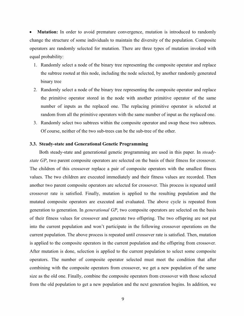
• Mutation: In order to avoid premature convergence, mutation is introduced to randomly
change the structure of some individuals to maintain the diversity of the population. Composite
operators are randomly selected for mutation. There are three types of mutation invoked with
equal probability:
1. Randomly select a node of the binary tree representing the composite operator and replace
the subtree rooted at this node, including the node selected, by another randomly generated
binary tree
2. Randomly select a node of the binary tree representing the composite operator and replace
the primitive operator stored in the node with another primitive operator of the same
number of inputs as the replaced one. The replacing primitive operator is selected at
random from all the primitive operators with the same number of input as the replaced one.
3. Randomly select two subtrees within the composite operator and swap these two subtrees.
Of course, neither of the two sub-trees can be the sub-tree of the other. 3.3. Steady-state and Generational Genetic Programming
Both steady-state and generational genetic programming are used in this paper. In steady-
state GP, two parent composite operators are selected on the basis of their fitness for crossover.
The children of this crossover replace a pair of composite operators with the smallest fitness
values. The two children are executed immediately and their fitness values are recorded. Then
another two parent composite operators are selected for crossover. This process is repeated until
crossover rate is satisfied. Finally, mutation is applied to the resulting population and the
mutated composite operators are executed and evaluated. The above cycle is repeated from
generation to generation. In generational GP, two composite operators are selected on the basis
of their fitness values for crossover and generate two offspring. The two offspring are not put
into the current population and won’t participate in the following crossover operations on the
current population. The above process is repeated until crossover rate is satisfied. Then, mutation
is applied to the composite operators in the current population and the offspring from crossover.
After mutation is done, selection is applied to the current population to select some composite
operators. The number of composite operator selected must meet the condition that after
combining with the composite operators from crossover, we get a new population of the same
size as the old one. Finally, combine the composite operators from crossover with those selected
from the old population to get a new population and the next generation begins. In addition, we
9

adopt an elitism replacement method that keeps the best composite operator from generation to
generation.
• Steady-state Genetic Programming:
0. randomly generate population P of size M and evaluate each composite operator in P.
1. for gen = 1 to N do // N is the number of generation
2. keep the best composite operator in P.
3. repeat
4. select 2 composite operators from P based on their fitness values for crossover.
5. select 2 composite operators with the lowest fitness values in P for replacement.
6. perform crossover operation and let the 2 offspring replace the 2 composite
operators selected for replacement.
7. execute the 2 offspring and evaluate their fitness values.
8. until crossover rate is met.
9. perform mutation on each composite operator with probability of mutation_rate and
evaluate mutated composite operators.
10. After crossover and mutation, a new population P’ is generated.
11. let the best composite operator from population P replace the worst composite operator in
P’ and let P = P’.
12. if the fitness value of the best composite operator in P is above fitness threshold value
then
13. stop.
endif
14. check each composite operator in P. if its size exceeds the size limit and it is not the best
composite operator in P, replace it with one of its subtree whose size is within the size
limit.
endfor // loop 1
• Generational Genetic Programming:
0. randomly generate populations of size M and evaluate each composite operator in P.
1. for gen = 1 to N do // N is the number of generation
2. keep the best composite operator in P.
10

3. perform crossover on the composite operators in P until crossover rate is satisfied and
keep all the offspring from crossover separately.
4. perform mutation on the composite operators in P and the offspring from crossover with
the probability of mutation rate.
5. perform selection on P to select some composite operators. The number of selected
composite operator must be M minus the number of composite operators from crossover.
6. combine the composite operators from crossover with those from P to get a new
population P’ of the same size as P.
7. evaluate offspring from crossover and the mutated composite operators.
8. let the best composite operator from P replace the worst composite operator in P’ and
let P = P’.
9. if the fitness of the best composite operator in P is above fitness threshold then
10. stop.
endif
11. check each composite operator in P. if its size exceeds the size limit and it is not the best
composite operator in P, replace it with one of its subtree whose size is within the size
limit.
endfor // loop 1 4. Experiments
Various experiments are performed to test the efficacy of genetic programming in
extracting regions of interest from real synthetic aperture radar (SAR) images, infrared (IR)
images and RGB color images. The size of SAR images is 128×128, except the tank SAR
images whose size is 80×80, and the size of IR and RGB color images is 160×120. GP (in
subsections 4.1 and 4.2) is not applied to the whole training image, but only to a region or
regions carefully selected from the training image, to generate the composite operators. The
generated composite operator is then applied to the whole training image and to some other
testing images to evaluate it. The advantage of performing training on a small selected region is
that it can greatly reduce the training time, making it practical for the GP system to be used as a
subsystem of other learning systems, which improve the efficiency of GP by adapting the
parameters of GP system based on its performance. Our experiments show that if the training
11

regions are carefully selected from the training images, the best composite operator generated by
GP is effective. In the following experiments in sections 4.1 and 4.2, the parameters are:
population size (100), the number of generations (70), the fitness threshold value (1.0), the
crossover rate (0.6), the mutation rate (0.05), the maximum size of composite operator (30), and
the segmentation threshold (0). In each experiment, GP is invoked ten times with the same
parameters and the same training region(s). The coordinate of the upper left corner of an image
is (0, 0). The ground truth is used only during training, it is not needed during testing. We use it
in testing only for evaluating the performance of the composite operator on testing images. 4.1. SAR images
Five experiments are performed with real SAR images. The experimental results from one
run and the average performance of ten runs are reported in Table 3. We select the run in which
GP finds the best composite operator among the composite operators found in all ten runs. The
first two rows show the fitness value of the best composite operator and the population fitness
value (average fitness value of all the composite operators in the population) on training
region(s) in the initial and final generations in the selected run. The numbers in the parenthesis in
the “fop” columns are the fitness values of the best composite operators on the whole training
image (numbers with a * superscript) and other testing images in their entirety. The last two
rows show the average values of the above fitness values over all ten runs. The regions extracted
during the training and testing by the best composite operator from the selected run are shown in
the following examples.
Table 3. The performance of our approach on various examples of SAR images. (fop = fitness of the best composite operator, fp = fitness of population, *: indicate fitness on training images, finitial = fitness in the initial generation, ffinal = fitness in the final population)
fi
f
Afi
Af
Road Lake River Field Tank
fop fp fop fp fop fp fop fp fop fp
nitial 0.68 0.28 0.56 0.32 0.65 0.18 0.53 0.39 0.51 0.16
final
0.95 (0.93*,
0.9, 0.93)
0.67 0.97
(0.93*, 0.98)
0.930.90
(0.71*, 0.83)
0.850.78
(0.89*, 0.80)
0.64 0.88
(0.88*, 0.84)
0.80
ve. nitial 0.55 0.27 0.59 0.32 0.48 0.18 0.54 0.37 0.61 0.17
ve. 0.83 0.60 0.95 0.92 0.85 0.77 0.76 0.59 0.86 0.68
final12

• Example 1 Road Extraction: Three images contain road, the first one contains
horizontal paved road and field (Fig 1(a)); the second one contains unpaved road and field (Fig
8(a)); the third one contains vertical paved road and grass (Fig 8(d)). Training is done on the
training regions of training image shown in Figure 1(a) and testing is performed on the whole
training image and testing images. There are two training regions, locating from (5, 19) to (50,
119) and from (82, 48) to (126, 124), respectively. Figure 1(b) shows the ground truth provided
by the user and the training regions. The white region corresponds to the road and only the
training regions of the ground truth are used in the evaluation during the training. Figure 2 shows
the sixteen primitive feature images of the training image.
(c) composite feature image (b) ground truth (d) ROI extracted(a) paved road vs. field
Figure 1. Training SAR image containing road.
PFIM0 PFIM7PFIM6 PFIM5PFIM4PFIM3PFIM2 PFIM1
PFIM8 PFIM10 PFIM12 PFIM14 PFIM9 PFIM11 PFIM13 PFIM15 Figure 2. Sixteen primitive feature images of training SAR image containing road.
The generational GP is used to synthesize a composite operator to extract the road and the
results of the 6th run are reported. The fitness value of the best composite operator in the initial
population is 0.68 and the population fitness value is 0.28. The fitness value of the best
composite operator in the final population is 0.95 and the population fitness value is 0.67. Figure
1(c) shows the output image of the best composite operator on the whole training image and
Figure 1(d) shows the binary image after segmentation. The output image has both positive
pixels in brighter shade and negative pixels in darker shade. Positive pixels belong to the region
13

to be extracted. The fitness value of the extracted ROI is 0.93. The best composite operator has
17 nodes and its depth is 16. It has only one leaf node containing 5×5 median image. The median
image is less noisy, since median filtering is effective in eliminating speckle noises. The best
composite operator is shown in Figure 3, where PFIM14 is 5×5 median image. Figure 4 shows
how the average fitness of the best composite operator and average fitness of population over all
10 runs change as GP explore the composite operator space. Unlike [6] where the population
fitness approaches the fitness of the best composite operator as GP proceeds, in Figure 4,
population fitness is much lower than that of best composite operator even at the end of GP
search. It is reasonable, since we don’t restrict the selection of crossover points. The population
fitness is not important since only the best composite operator is used in testing. If GP finds one
effective composite operator, the GP learning is successful. The large difference between the
fitness of the best composite operator and the population indicates that the diversity of the
population is always maintained during GP search, which is very helpful in preventing
premature convergence. 10 best composite operators are learned in 10 runs.
After computing the percentage of each primitive operator and primitive feature image
among the total number of internal node (representing primitive operator) and total number leaf
node (representing primitive feature image), we get the utility of these primitive operators and
primitive feature images, which is shown in Figure 5(a) and (b). MED (primitive operator 15)
and PFIM5 (the 6th primitive feature image) have the highest frequency of utility. Figure 6 shows
the output image of each node of the best composite operator shown in Figure 3. From left to
right and top to bottom, the images correspond to nodes sorted in the pre-traversal order of the
binary tree representing the best composite operator. The output of the root node is shown in
Figure 1(c), so Figure 6 shows the outputs of other nodes. The primitive operators in Figure 6 are
connected by arrow. The operator at the tail of an arrow provides input to the operator at the
head of the arrow. After segmenting the output image of a node, we get the ROI (shown as the
white region) extracted by the corresponding subtree rooted at the node. The extracted ROIs and
their fitness values are shown in Figure 7. If an output image of a node has no positive pixel (for
example, the output of MEAN primitive operator), nothing is extracted and the fitness value is 0;
if an output image has positive pixels only (for example, PFIM14 has positive pixels only),
everything is extracted and the fitness is 0.25. The output of the root node storing primitive
operator MED is shown in Figure 1(d).
14

0.2
0.4
0.6
0.8
1
0 5 10 15 20 25 30 35 40 45 50 55 60 65 70
generation
fitne
ss
best
population
population
PFIM14 MAX
DIVCDIVC MULC MAX MULC
MEANSQRT MAXADDC MULC
MAXMULC MAXMAXMED
Figure 3. Learned composite operator tree. Figure 4. Fitness versus generation (road vs. field).
0
0.2
0.4
0.6
1 3 5 7 9 11 13 15 17
(a) primitive operator
utili
ty
00.10.20.30.4
0 1 2 3 4 5 6 7 8 9 10 11 12 13 14 15
(b) primitive feature image
utili
ty
Figure 5. Utility of primitive operators and primitive feature images.
PFIM14MAXDIVCDIVCMULCMAXMULCMEAN
SQRTMAXADDCMULCMAXMULCMAXMAX
Figure 6. Feature image output by the nodes of the best composite operator.
PFIM14 0.25
MAX 0.25
DIVC 0.25
DIVC 0
MULC0.25
MAX 0.25
MULC 0
MEAN 0
SQRT0
MAX 0
ADDC 0.68
MULC 0.09
MAX 0.12
MULC 0.52
MAX 0.76
MAX 0.93
Figure 7. ROI extracted from the output image of nodes of the best composite operator. (The fitness value is shown for the entire image.)
15

We applied the composite operator obtained in the above training to the other two real SAR
images shown in Figure 8(a) and 8(d). Figure 8(b) and 8(e) show the output of the composite
operator and Figure 8(c) shows the region extracted from Figure 8(a). The fitness value of the
region is 0.90. Figure 8(f) shows the region extracted from Figure 8(d) and the fitness value of
the region, which is 0.93.
(d) paved road vs. grass
(e) composite feature image
(f) ROI extracted
(a) unpaved road vs. field
(b) composite feature image
(c) ROI extracted
Figure 8. Testing SAR image containing road. • Example 2 Lake Extraction: Two SAR images contain lake (Fig 9(a), 10(a)), the first
one contains a lake and field, and the second one contains a lake and grass. Figure 9(a) shows
the original training image containing lake and field and the training region from (85, 85) to
(127, 127). Figure 5(b) shows the ground truth provided by the user. The white region
corresponds to the lake to be extracted. Figure 10(a) shows the image containing lake and grass.
(c) composite feature image (b) ground truth (d) ROI extracted(a) lake vs. field Figure 9. Training SAR image containing lake. The steady-state GP is used to generate the composite operator and the results of the 9th run
are reported. The fitness value of the best composite operator in the initial population is 0.56 and
the population fitness value is 0.32. The fitness value of the best composite operator in the final
population is 0.97 and the population fitness value is 0.93. Figure 9(c) shows the output image of
the best composite operator on the whole training image and Figure 9(d) shows the binary image
after segmentation. The fitness value of the extracted ROI is 0.93.
We apply the composite operator to the testing image containing lake and grass. Figure 10(b)
shows the output of the composite operator and Figure 10(c) shows the region extracted from
Figure 10(a). The fitness of the region is 0.98.
16

(a) lake vs. grass (b) composite feature image (c) ROI extracted
Figure 10. Testing SAR image containing lake. • Example 3 River Extraction: Two SAR images contain river and field. Figure 11(a) and
11(b) show the original training image and the ground truth provided by the user. The white
region in Figure 11(b) corresponds to the river to be extracted. The training regions are from (68,
31) to (126, 103) and from (2, 8) to (28, 74). The testing SAR image is shown in Figure 14(a).
(c) composite feature image (b) ground truth (d) ROI extracted(a) river vs. field
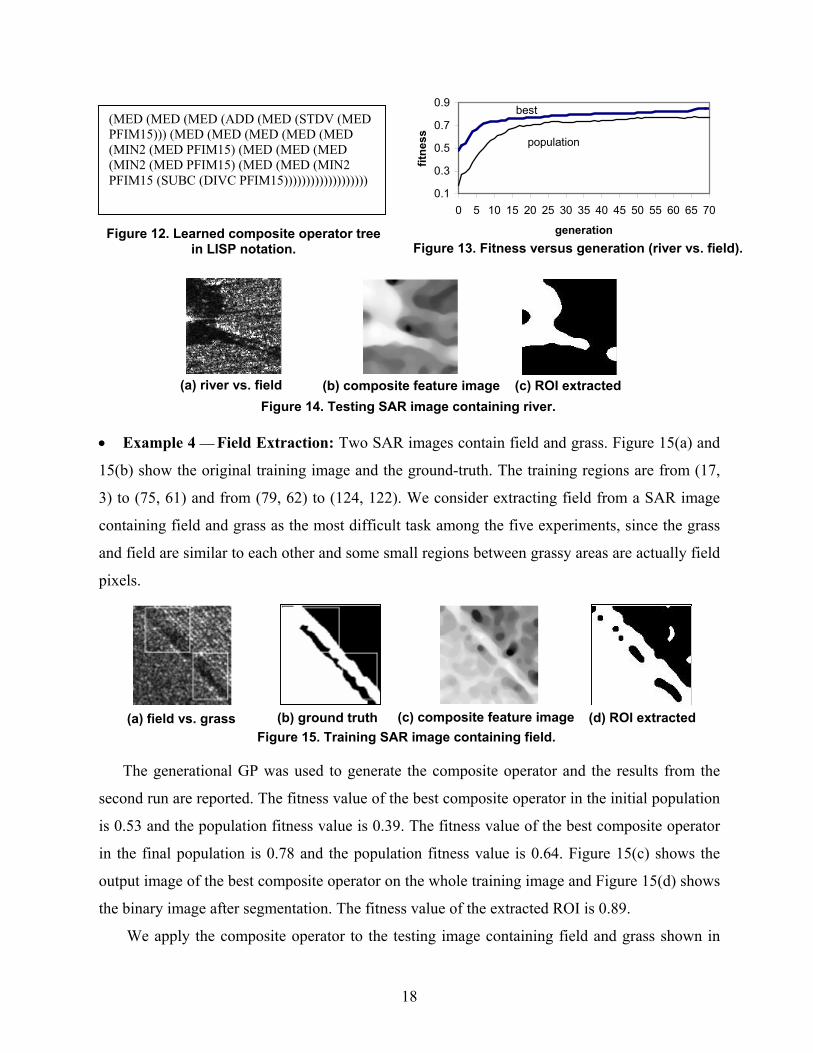
Figure 11. Training SAR image containing river. The steady-state GP was used to generate the composite operator and the results from the
fourth run are reported. The fitness value of the best composite operator in the initial population
is 0.65 and the population fitness value is 0.18. The fitness value of the best composite operator
in the final population is 0.90 and the population fitness value is 0.85. Figure 11(c) shows the
output image of the best composite operator on the whole training image and Figure 11(d) shows
the binary image after segmentation. The fitness value of the extracted ROI is 0.71. The best
composite operator has 29 nodes and its depth is 19. It has five leaf nodes and all contain 7×7
median image. There are more than ten MED operators that are very useful in eliminating
speckle noises. It is shown in Figure 12. Figure 13 shows how the average fitness of the best
composite operator and average fitness of population over all 10 runs change as GP explores the
composite operator space.
We apply the composite operator to the testing image containing a river and field. Figure
14(b) shows the output of the composite operator and Figure 14(c) shows the region extracted
from Figure 14(a) and the fitness value of the region is 0.83. There are some islands in the river
and these islands along with the river around them are not extracted.
17
0.1
0.3
0.5
0.7
0.9
0 5 10 15 20 25 30 35 40 45 50 55 60 65 70
generation
fitne
ss
best
population
(MED (MED (MED (ADD (MED (STDV (MED PFIM15))) (MED (MED (MED (MED (MED (MIN2 (MED PFIM15) (MED (MED (MED (MIN2 (MED PFIM15) (MED (MED (MIN2 PFIM15 (SUBC (DIVC PFIM15)))))))))))))))))))
Figure 12. Learned composite operator tree in LISP notation. Figure 13. Fitness versus generation (river vs. field).
(a) river vs. field (b) composite feature image (c) ROI extracted
Figure 14. Testing SAR image containing river. • Example 4 Field Extraction: Two SAR images contain field and grass. Figure 15(a) and
15(b) show the original training image and the ground-truth. The training regions are from (17,
3) to (75, 61) and from (79, 62) to (124, 122). We consider extracting field from a SAR image
containing field and grass as the most difficult task among the five experiments, since the grass
and field are similar to each other and some small regions between grassy areas are actually field
pixels.
(c) composite feature image (b) ground truth (d) ROI extracted(a) field vs. grass
Figure 15. Training SAR image containing field.
The generational GP was used to generate the composite operator and the results from the
second run are reported. The fitness value of the best composite operator in the initial population
is 0.53 and the population fitness value is 0.39. The fitness value of the best composite operator
in the final population is 0.78 and the population fitness value is 0.64. Figure 15(c) shows the
output image of the best composite operator on the whole training image and Figure 15(d) shows
the binary image after segmentation. The fitness value of the extracted ROI is 0.89.
We apply the composite operator to the testing image containing field and grass shown in
18

Figure 16(a). Figure 16(b) shows the output of the composite operator and Figure 16(c) shows
the region extracted from Figure 16(a). The fitness value of the region is 0.80.
(a) field vs. grass (b) composite feature image (c) ROI extracted Figure 16. Testing SAR image containing field. • Example 5 Tank Extraction: We use SAR images of T72 tank that are taken under
different depression and azimuth angles and the size of the images is 80×80. The training image
contains T72 tank under depression angle 17° and azimuth angle 135°, which is shown in Figure
17(a). The training region is from (19, 17) to (68, 66). The testing SAR image contains a T72
tank under depression angle 20° and azimuth angle 225°, which is shown in Figure 20(a). The
ground-truth is shown in Figure 17(b).
(c) composite feature image (b) ground truth (d) ROI extracted(a) T72 tank
Figure 17. Training SAR image containing field.
The generational GP is applied to synthesize composite operators for tank detection and the
results from the first run are reported. The fitness value of the best composite operator in the
initial population is 0.51 and the population fitness value is 0.16. The fitness value of the best
composite operator in the final population is 0.88 and the population fitness value is 0.80. Figure
17(c) shows the output image of the best composite operator on the whole training image and
Figure 17(d) shows the binary image after segmentation. The fitness value of the extracted ROI
is 0.88. The best composite operator has 10 nodes and its depth is 9. It has only one leaf node,
which contains the 5×5 mean image. It is shown in Figure 18. Figure 19 shows how the average
fitness of the best composite operator and average fitness of population over all 10 runs change
as GP proceeds.
19

0.1
0.3
0.5
0.7
0.9
0 5 10 15 20 25 30 35 40 45 50 55 60 65 70
generation
fitne
ss
best
population
(MED (SQRT (MULC (MULC (SUBC (MULC (SQRT (SUBC (SQRT PFIM2)))))))))
Figure 18. Learned composite operator tree in LISP notation.
Figure 19. Fitness versus generation (T72 tank).
We apply the composite operator to the testing image containing T72 tank under depression
angle 20° and azimuth angle 225°. Figure 20(b) shows the output of the composite operator and
Figure 20(c) shows the region corresponding to the tank. The fitness of the extracted ROI is
0.84. Our results show that GP is very much capable of synthesizing composite operators for
target detection. With more and more SAR images collected by satellites and airplanes, it is
impractical for human experts to scan each SAR image to find targets. Applying the synthesized
composite operators on these images, regions containing potential targets can be quickly
detected and passed on to automatic target recognition systems or to human experts for further
examination. Concentrating on the regions of interest, the human experts and recognition
systems can perform recognition task more effectively and more efficiently. (a) T72 tank (b) composite feature image (c) ROI extracted Figure 20. Testing SAR image containing tank. 4.2. IR and RGB Color Images
One experiment is performed with IR images and one is performed with RGB color images.
The experimental results from one run and the average performance of ten runs are reported in
Table 4. As we did in Subsection 4.1, we select the run in which GP finds the best composite
operator among the composite operators found in all the ten runs. The regions extracted during
the training and testing by the best composite operator from the selected run are shown in the
following examples.
20

Table 4. The performance of our approach on examples of IR and RGB color images. (fop = fitness of the best composite operator, fp = fitness of population, *: indicate fitness on training
images, finitial = fitness in the initial generation, ffinal = fitness in the final population)
fi
f
Ave
Ave
• People Extr
in the scene. W
testing. Figure
training regions
training region
training is that
Nothing in this
defined as one m
fitness value is
during training.
fitness is compu
ROI, as we did
(d) and (g).
The generatio
results from the
initial populatio
composite opera
21(c) shows the
Figure 21(d) sho
is 0.85. The bes
is shown in Fig
IR Image People Color Image Car
fop fp fop fp
nitial 0.56 0.23 0.35 0.18
final 0.93 (0.85*, 0.84, 0.81, 0.86) 0.79
0.84 (0.82*, 0.76) 0.79
. finitial 0.59 0.21 0.47 0.18 . ffinal 0.85 0.65 0.72 0.67
action in IR Images: In IR images, pixel values correspond to the temperature
e have four IR images with one used in training and the other three used in
21(a) and (b) show the training image and the ground truth. There are two
from (59, 9) to (106, 88) and from (2, 3) to (21, 82), respectively. The left
contains no pixel belonging to the person. The reason for selecting it during
there are major changes of pixel intensities among the pixels in the region.
region should be detected. The fitness of composite operator on this region is
inus the percentage of pixels detected in the region. If nothing is detected, the
1.0. Averaging the fitness values on the two training regions, we get the fitness
When the learned composite operator is applied to the whole training image, the
ted as a measurement of the overlap between the ground truth and the extracted
in the previous experiments. Three testing IR images are shown in Figure 24(a),
nal GP is applied to synthesize composite operators for person detection and the
third run are reported. The fitness value of the best composite operator in the
n is 0.56 and the population fitness value is 0.23. The fitness value of the best
tor in the final population is 0.93 and the population fitness value is 0.79. Figure
output image of the best composite operator on the whole training image and
ws the binary image after segmentation. The fitness value of the extracted ROI
t composite operator has 28 nodes and its depth is 13. It has nine leaf nodes and
ure 22. Figure 23 shows how the average fitness of the best composite operator
21

and average fitness of population over all the 10 runs change as GP proceeds.
(c) composite feature image (b) ground truth (d) ROI extracted(a) person
Figure 21. Training IR image containing person.
0.2
0.4
0.6
0.8
0 5 10 15 20 25 30 35 40 45 50 55 60 65 70
generation
fitne
ss
best
population
(SQRT (SQRT (SUBC (SQRT (MAX2 (MAX2 PFIM1 (SUB (MAX2 PFIM14 PFIM15) (DIV (MULC (SQRT (MAX (MAX (ADD PFIM12 PFIM15))))) PFIM9))) (DIV (MULC (SQRT (MAX (ADD PFIM12 PFIM9)))) PFIM9))))))
Figure 22. Learned composite operator tree in LISP notation.
Figure 23. Fitness versus generation (T72 tank). (c) ROI extracted(a) person (b) composite feature image
(f) ROI extracted (d) person (e) composite feature image (i) ROI extracted (g) person (h) composite feature image
Figure 24. Testing IR images containing person. We apply the composite operator to the testing images shown in Figure 24. Figure 24(b), (e)
and (h) show the output of the composite operator and Figure 24(c), (f) and (i) show the ROI
extracted. Their fitness values are 0.84, 0.81 and 0.86 respectively.
22

• Car Extraction in RGB Color Image: GP is applied to learn features to detect car in RGB
color images. Unlike previous experiments, the primitive feature images in this experiment are
RED, GREEN and BLUE planes of RGB color image. Figure 25(a), (b) and (c) show the RED,
GREEN and BLUE planes of the training image. The ground truth is shown in Figure 25(d). The
training region is from (21, 3) to (91, 46). (a) RED plane (b) GREEN plane (c) BLUE plane (f) ROI extracted (e) composite feature image (d) ground truth Figure 25. Training RGB color image containing car. The steady-state GP is applied to synthesize composite operators for car detection and the
results from the fourth run are reported. The fitness value of the best composite operator in the
initial population is 0.35 and the population fitness value is 0.18. The fitness value of the best
composite operator in the final population is 0.84 and the population fitness value is 0.79. Figure
25(e) shows the output image of the best composite operator on the whole training image and
Figure 25(f) shows the binary image after segmentation. The fitness value of the extracted ROI
is 0.82. The best composite operator has 44 nodes and its depth is 21. It has ten leaf nodes with
one of them containing GREEN plane and the others contain BLUE plane. It is shown in Figure
26, where PFG means GREEN plane and PFB means BLUE plane. Figure 27 shows how the
average fitness of the best composite operator and average fitness of population over all 10 runs
change as GP proceeds.
Figure 26. Learned composite operator tree in LISP notation.
0.10.30.50.70.9
0 5 10 15 20 25 30 35 40 45 50 55 60 65 70
generation
fitne
ss
bestpopulation
(MED (MED (MED (MULC (MUL (SUB (MIN (MEAN (MAX2 (MED (ADDC (MAX2 (ADDC (ADDC (MED (MAX2 (MED (MED (MAX2 (MED (ADDC PFB)) PFB))) PFB)))) PFB))) (MED PFG)))) (ADDC (MAX2 (ADDC (ADDC (MED (MAX2 (MED (MED (MAX2 (MED (ADDC PFB))PFB))) PFB)))) PFB))) (ADDC PFB
))))))
Figure 27. Fitness versus generation (T72 tank).
23

We apply the composite operator to the testing image whose RED plane is shown in Figure
28(a). Figure 28(b) shows the output of the composite operator and Figure 28(c) shows the ROI
extracted. The fitness value of extracted ROI is 0.76.
(c) ROI extracted (b) composite feature image (a) RED plane Figure 28. Testing RGB color image containing car. 4.3. Comparison In [6], we applied genetic programming to learn composite operators for object detection.
This paper is an advancement to our previous work. The major differences between the method
presented here and that in [6] are:
1) Unlike [6] where a whole training image is used during training, GP runs on carefully
selected region(s) in this paper to reduce the training time.
2) Hard size limit on the composite operator is replaced by soft size limit in this paper.
This removes the restriction on the selection of crossover point in the parent composite
operators to improve the search efficiency of GP, as stated in subsection 3.2.
3) Only the first mutation type in subsection 3.2 and only the fist seven primitive feature
images are used in [6]. With more mutation types and more primitive feature images
used, the diversity of the composite operator population can be further increased.
We summarize the experimental results on REAL SAR images in [6] for the purpose of
comparison. The parameters are: population size (100), the number of generations (100), the
fitness threshold value (1.0), the crossover rate (0.6), the mutation rate (0.1), the maximum size
(number of internal node) of composite operator (30), and the segmentation threshold (0). In
each experiment, GP is invoked ten times with the same parameters. The experimental results
from one run and the average performance of ten runs are reported in Table 5. We select the run
in which GP finds the best composite operator among the composite operators found in all ten
runs to report. The numbers in the parenthesis in the “fop” columns are the fitness values of the
best composite operators on the testing SAR images.
24

t
•
im
fit
fit
0.
co
ap
Fi
fr
ou
va
(f
•
im
be
Table 5. The Performance of Genetic Programming on Various Examples of SAR Images.
(fop = fitness of the best composite operator, fp = fitness of population, *: indicate fitness on raining images, finitial = fitness in the initial generation, ffinal = fitness in the final population)
Ro
ages
ness
ness
92 an
mpo
plied
gure
om F
tput
lue o
fi
f
Ave
Ave
a) coeatur
La
age.
st co
Road Lake River Field
fop fp fop fp fop fp fop fp
nitial 0.47 0.19 0.65 0.42 0.43 0.21 0.62 0.44
final 0.92* (0.92, 0.89) 0.89
0.93* ( 0.92 ) 0.92
0.74* ( 0.84 ) 0.68
0.87* ( 0.68 ) 0.86
. finitial 0.47 0.18 0.73 0.39 0.37 0.11 0.65 0.41
. ffinal 0.81 0.76 0.92 0.87 0.68 0.58 0.84 0.77
ad Extraction: Figure 1(a) shows the training image and Figure 8(a), (d) show the testing
. The generational GP was used to generate a composite operator to extract the road. The
value of the best composite operator in the initial population is 0.47 and the population
value is 0.19. The fitness value of the best composite operator in the final population is
d the population fitness value is 0.89. Figure 29(a) shows the output image of the best
site operator in the final population and Figure 29(b) shows the extracted ROI. We
the composite operator obtained in the above training to the two testing SAR images.
29(c) and (d) show the output image of the composite operator and the ROI extracted
igure 8(a). The fitness value of the extracted ROI is 0.92. Figure 29(e) and (f) show the
image of the composite operator and the ROI extracted from Figure 8(d). The fitness
f the extracted ROI is 0.89.
(e) composite feature image
(f) ROI extracted from Figure 8(d)
mposite e image
(c) composite feature image
(b) ROI extracted from Figure 1(a)
(d) ROI extracted from Figure 8(a)
Figure 29. Results on SAR images containing road.
ke Extraction: Figure 9(a) shows the training image and Figure 10(a) shows the testing
The steady-state GP was used to generate the composite operator. The fitness value of the
mposite operator in the initial population is 0.65 and the population fitness value is 0.42.
25

The fitness value of the best composite operator in the final population is 0.93 and the population
fitness value is 0.92. Figure 30(a) shows the output image of the best composite operator in the
final population and Figure 30(b) shows the extracted ROI. We applied the composite operator
to the testing SAR image. Figure 30(c) and (d) show the output image of the composite operator
and the extracted ROI with fitness value 0.92. In Figure 30(a) and (c), pixels in the small dark
regions have very low pixel values (negative values with very large absolute value), thus,
making many pixels near the borders of the image appear bright, although these pixels have
negative pixel values.
(a) composite feature
image (b) ROI extracted from Figure 5(a)
(d) ROI extracted from Figure 6(a)
(c) composite feature image
Figure 30. Results on SAR images containing lake.
• River Extraction: Figure 11(a) shows the training image and Figure 14(a) shows the testing
image. The steady-state GP was used to generate the composite operator. The fitness value of the
best composite operator in the initial population is 0.43 and the population fitness value is 0.21.
The fitness value of the best composite operator in the final population is 0.74 and the population
fitness value is 0.68. Figure 31(a) shows the output image of the best composite operator in the
final population and Figure 31(b) shows the extracted ROI. We applied the composite operator
to the testing image. Figure 31(c) and (d) show the output image of the composite operator and
the extracted ROI with fitness value 0.84. Like Figure 30(c), pixels in the small dark region have
very low pixel values (negative values with very large absolute value), thus, making many pixels
with negative pixel values appear bright,
(a) composite feature
image (b) ROI extracted from Figure 7(a)
(d) ROI extracted from Figure 10(a)
(c) composite feature image
Figure 31. Results on SAR images containing river.
26

• Field Extraction: Figure 15(a) shows the training image and Figure 16(a) shows the testing
image. The generational GP was used to generate the composite operator. The fitness value of
the best composite operator in the initial population is 0.62 and the population fitness value is
0.44. The fitness value of the best composite operator in the final population is 0.87 and the
population fitness value is 0.86. Figure 32(a) shows the output image of the best composite
operator in the final population and Figure 32(b) shows the extracted ROI. We applied the
composite operator to the testing image. Figure 32(c) and (d) show the output image of the
composite operator and the extracted ROI with fitness value 0.68.
(a) composite feature
image (b) ROI extracted from Figure 11(a)
(d) ROI extracted from Figure 12(a)
(c) composite feature image
Figure 32. Results on SAR images containing field.
From Tables 3 and 5 and associated figures, it can be seen that if the training regions are
carefully selected and represent the characteristics of training images, the composite operators
learned by GP running on training regions are effective in extracting the ROIs containing the
object and their performances are comparable to the performances of composite operators
learned by GP running on the whole training images. By running on the selected regions, the
training time is greatly reduced. Table 6 shows the average running time of GP running on
selected regions (Region GP) and GP running on the whole training images (Image GP) over all
ten runs and the time is measured in second. Since the number of generation in [6] is 100 and the
number of generation in this paper is 70, the running time of “Image GP” in Table 6 is the
actually running time of “Image GP” times 0.7. It can be seen that the training time using
selected training region is much shorter than that using the whole image.
Table 6. Average running time of Region GP and Image GP.
Regi
Ima
Road Lake River Field
on GP 12876 2263 6560 9685
ge GP 23608 9120 66476 21485
27

5. Conclusions
In this paper, we use genetic programming to synthesize composite operators and composite
features to detect potential objects in images. We use soft composite operator size limit to avoid
code-bloating and severe restriction on GP search. Our experimental results show that the
primitive operators and primitive features defined by us are effective. GP can synthesize
effective composite operators for object detection by running on the carefully selected training
regions of training image and the synthesized composite operators can be applied to the whole
training image and other similar testing images. We don’t find significant difference between
generational and steady-state genetic programming algorithms. GP has well known code bloat
problem. Controlling code bloat due to the limited computational resources inevitably restricts
the search efficiency of GP. How to reach the balance point between these two conflicting
factors is critical in the implementation of GP. In the future, we plan to address this problem by
designing new fitness functions based on the minimum description length (MDL) principle to
incorporate the size of composite operator into the evaluation process. Also, we will extend this
work by discovering features within the regions of interest for automated object recognition.
Acknowledgement: This research is supported by the grant F33615-99-C-1440. The contents of
the information do not necessarily reflect the position or policy of the U. S. government. Reference
[1] A. Ghosh and S. Tsutsui (Eds.), Advances in Evolutionary Computing – Theory and
Application, Springer-Verlag, 2003.
[2] B. Bhanu et al. (Eds), IEEE Trans. on Image Processing – Special Issue on Automatic
Target Recognition, Vol. 6, No. 1, Jan 1997.
[3] J. R. Koza, Genetic Programming II: Automatic Discovery of Reusable Programs, MIT
Press, 1994.
[4] C. Harris and B. Buxton, “Evolving edge detectors with genetic programming,” Proc.
Genetic Programming, 1st Annual Conference, Cambridge, MA, USA, pp. 309-314, MIT
Press, 1996.
[5] R. Poli, “Genetic programming for feature detection and image segmentation,” in
Evolutionary Computation, T. C. Forgarty Ed., pp. 110-125, 1996.
[6] B. Bhanu and Y. Lin, “Learning composite operators for object detection”, Proc. Genetic
28

29
and Evolutionary Computation Conference, pp. 1003-1010, July, 2002.
[7] S. A. Stanhope and J. M. Daida, “Genetic programming for automatic target classification
and recognition in synthetic aperture radar imagery,” Proceeding Conference. Evolutionary
Programming VII, pp. 735-744, 1998.
[8] D. Howard, S. C. Roberts, and R. Brankin, “Target detection in SAR imagery by genetic
programming,” Advances in Engineering Software, vol. 30, no. 5, pp. 303-311, Elsevier,
May 1999.
[9] S. C. Roberts and D. Howard, “Evolution of vehicle detectors for infrared line scan
imagery,” Proc. Evolutionary Image Analysis, Signal Processing and Telecommunications,
First European Workshops, EvoIASP’99 and EuroEcTel’99, Berlin, Germany, pp. 110-125,
Springer-Verlag, 1999.
[10] B. Bhanu and S. Fonder, “Learning-integrated interactive image segmentation,” chapter in
Advances in Evolutionary Computing – Theory and Application, A. Ghosh and S. Tsutsui
(Eds.), pp. 863 – 895, Springer-Verlag, 2003.