Object-Based Land Cover ClassificationUsing High-Posting-Density LiDAR Data

Jungho Im1

Environmental Resources and Forest Engineering, State University of New York, College of Environmental Sciences and Forestry, One Forestry Drive, Syracuse, New York 13210

John R. Jensen and Michael E. HodgsonDepartment of Geography, University of South Carolina, Columbia, South Carolina 29208

Abstract: This study introduces a method for object-based land cover classificationbased solely on the analysis of LiDAR-derived information—i.e., without the use ofconventional optical imagery such as aerial photography or multispectral imagery.The method focuses on the relative information content from height, intensity, andshape of features found in the scene. Eight object-based metrics were used to clas-sify the terrain into land cover information: mean height, standard deviation(STDEV) of height, height homogeneity, height contrast, height entropy, height cor-relation, mean intensity, and compactness. Using machine-learning decision trees,these metrics yielded land cover classification accuracies > 90%. A sensitivity analy-sis found that mean intensity was the key metric for differentiating between thegrass and road/parking lot classes. Mean height was also a contributing discrimina-tor for distinguishing features with different height information, such as between thebuilding and grass classes. The shape- or texture-based metrics did not significantlyimprove the land cover classifications. The most important three metrics (i.e., meanheight, STDEV height, and mean intensity) were sufficient to achieve classificationaccuracies > 90%.

INTRODUCTION

LiDAR (Light Detection And Ranging) is an active optical remote sensing sys-tem that generally uses near-infrared laser light to measure the range from the sensorto a target on the Earth surface (Jensen, 2007). LiDAR range measurements can beused to identify the elevation of the target as well as its precise planimetric location.These two measurements are the fundamental building blocks for generating digitalelevation models (DEMs). Digital elevation information is a critical component inmost geographic information system (GIS) databases used by many agencies such asthe United States Geological Survey (USGS) and Federal Emergency Management

1Corresponding author; email: imj@esf.edu

209

GIScience & Remote Sensing, 2008, 45, No. 2, p. 209–228. DOI: 10.2747/1548-1603.45.2.209Copyright © 2008 by Bellwether Publishing, Ltd. All rights reserved.

210 IM ET AL.

Administration (FEMA). DEMs can be subdivided into: (1) digital surface models(DSMs) containing height information of the top “surface” of all features in the land-scape, including vegetation and buildings,; and (2) digital terrain models (DTMs)containing elevation information solely about the bare Earth (i.e., no above-surfaceheights) surface (Jensen, 2007).

Most LiDAR remote sensing systems that are used for terrestrial topographicmapping use near-infrared laser light from 1040 to 1060 nm, whereas blue-green laserlight (at approximately 532 nm) is used for bathymetric mapping due to its water pen-etration capability (Mikhail et al., 2001; Boland et al., 2004). Because each LiDARpoint is already georeferenced, LiDAR data can be directly used in spatial analysiswithout additional geometric correction (Flood and Gutelius, 1997; Jensen and Im,2007). Most LiDAR remote sensing systems now provide intensity information aswell as multiple returns representing surface heights. The return with the maximumenergy of all returned signals for a single pulse is usually recorded as the intensity forthat pulse (Baltsavias, 1999). Other factors such as gain setting, bidirectional effects,the angle of incidence, and atmospheric dispersion also influence the intensity valuesrecorded. Leonard (2005) points out that systems with automatic gain control adjustthe return signal gain in response to changes in target reflectance. Thus, such variabil-ity in intensity values can make it problematic to interpret or model the intensity data.

LiDAR data have been recently used in a variety of applications including topo-graphic mapping, forest and vegetation, and land cover classification. Some studieshave demonstrated the effectiveness of LiDAR for DEM-related terrain mapping(Hodgson et al., 2005; Toyra and Pietroniro, 2005; Raber et al., 2007). Manyresearchers have adopted LiDAR remote sensing for identifying vegetation structureand tree species (Hill and Thomson, 2005; Suarez et al., 2005; Bork and Su, 2007;Brandtberg, 2007). LiDAR data have also been used for land cover classification(Song et al., 2002; Hodgson et al., 2003; Lee and Shan, 2003; Rottensteiner et al.,2005).

Most previous research focused on integrating LiDAR data with other GIS-basedancillary data and/or remote sensing data such as multispectral imagery. LiDAR datahave been generally used as ancillary data to improve land cover classification accu-racy. Data fusion between LiDAR and other remote sensing data was a critical part ofthe studies. Some studies fused the data at a pixel level, whereas others performeddata fusion at a decision level. LiDAR data obtained at very high posting densities(i.e., < 0.5 m) increases its potential in a variety of applications. High-posting-densityLiDAR-derived information may be used to identify not only elevation of a landformbut also precise height and shape information of a target on the Earth’s surface such asvehicle or tree. The question then becomes, “Can such high-posting-density LiDARdata be used as the sole information source in applications such as image classifica-tion— without other ancillary data?”

This study explores the applicability of high-posting-density LiDAR data forland cover classifications with an object-based approach focusing on height infor-mation. For example, different land cover classes such as buildings and trees mayhave similar heights yet different shapes. Various height-related metrics such asmean, standard deviation, and textures were extracted for objects as well as a shapeindex, such as compactness. LiDAR-derived intensity data were also incorporated inthe analysis to determine its relative usefulness in land cover classification. In

OBJECT-BASED LAND COVER CLASSIFICATION 211

summary, the objectives of this study are to: (1) explore the applicability of high-posting-density LiDAR-derived features for land cover classification without incor-porating other remote sensing data, such as multispectral imagery; (2) evaluate thecapability of object-based metrics with machine-learning decision trees to classifythe LiDAR data; and (3) assess the sensitivity of each object-based metric for landcover classification.

METHODOLOGY

Study Area

The study area was located on the Savannah River National Laboratory (SRNL),a U.S. Department of Energy facility located near Aiken, SC. SRNL has: more than450 waste sites that store a variety of waste materials; a number of man-made struc-tures such as buildings and roads; water bodies; and forest (Mackey, 1998). Threestudy sites were selected to demonstrate the capability of high-posting-densityLiDAR data for land cover classification. Figure 1 shows the study sites on an ortho-photo (0.3 × 0.3 m spatial resolution) collected in 2001 along with the first returnLiDAR surface of the sites.

LiDAR Data Collection

LiDAR data were collected by Sanborn, LLC on November 14, 2004 using anOptech ALTM 2050 LiDAR sensor mounted on a Cessna 337 aircraft. The OptechALTM 2050 LiDAR sensor collected small footprint first and last returns (x, y, and z)and intensity data using a 1064 nm laser with a pulse repetition frequency (PRF) of 50kHz (Garcia-Quijano et al., 2007). Specifications for the high-posting-density LiDARdata collection are summarized in Table 1. Although the nominal posting spacing was0.4 m, the actual posting spacing was much finer due to the 70% overlap betweenmultiple flightlines, resulting in an observed posting density of 15.3 points/m2.

The LiDAR data were post-processed to yield x, y, and z coordinates for all firstand last returns. Last return data were processed to generate a “bare Earth” dataseteliminating obstructions on the ground using TerraModel’s TerraScan morphologicalfiltering software. The vertical accuracy of the LiDAR data was assessed to be 6 cmRMSE (Garcia-Quijano et al., 2007). A triangular irregular network (TIN) model was

Table 1. Summary of the Nominal LiDAR Data Collection Parameters

Nominal LiDAR data collection parameters

Date November 14, 2004Average altitude AGL 700 mAir speed 130 knotsFlightline sidelap 70%Nominal posting spacing 0.4 m

212 IM ET AL.

used to create the separate DTMs based on either first returns, last returns, bare Earth,or intensity point data. Four DSMs were then created from the TIN models at a spatialresolution of 25 cm. A local height surface was also created by subtracting the bareEarth surface from the first return surface.

Figure 2 depicts the flow diagram of the methodology used in the study. A totalof five surfaces (i.e., first returns, last returns, bare Earth, height, and intensity) weresubsequently used to identify image objects through the image segmentation process.Eight object-based metrics were extracted for use in a machine-learning decision treeclassification. Sensitivity analyses were conducted to determine which object-basedmetrics contributed most to the discrimination of land cover classes. Details aredescribed in the following sections.

Fig. 1. A. Three study sites of the Savannah River National Laboratory (SRNL). B. First returnLiDAR surface of Site A. C. First return LiDAR surface of Site B. D. First return LiDARsurface of Site C.

OBJECT-BASED LAND COVER CLASSIFICATION 213

Ground Reference Data

Two hundred ground reference points for each study site were randomly generatedfor the accuracy assessment using a sampling tool developed using Visual Basic in theArcGIS 9.x environment (Im, 2006). The land cover for each reference point was iden-tified through visual interpretation of a high-spatial-resolution aerial orthophoto andpersonal communication with SRNL on-site experts. The interpreted land cover wasassigned to one of five land classes: (1) building; (2) tree; (3) grass; (4) road/parkinglot; and (5) other artificial object. There were no trees in Site C. The other artificialobject class included vehicles, small storage containers (e.g., drums), and pipelines.

Image Segmentation

Definiens (former eCognition) software was used to segment image objectsbased on the five surface layers generated from the LiDAR returns: first returns, lastreturns, bare Earth, height, and intensity (Fig. 3). The segmentation process was abottom-up, region-merging approach where smaller objects were merged into larger

Fig. 2. Flow diagram of the methodology used in the study.

214 IM ET AL.

Fig. 3. Five layers used to generate image objects during the image segmentation process forSite A.

OBJECT-BASED LAND COVER CLASSIFICATION 215

objects based on three parameters (Baatz et al., 2004). A scale parameter determinedthe maximum allowable change of heterogeneity when several objects were merged(Benz et al., 2004). The segmentation process was terminated when the growth of anobject exceeded a scale parameter value. Greater values for the scale parameterresulted in larger objects. Five different scale parameters (i.e., 5, 10, 15, 20, and 25)were tested. A scale parameter of 10 was determined to be the best based on visualinterpretation of the resultant image segments.

Two more parameters were required to perform image segmentation: color/shapeand smoothness/compactness. The color/shape parameter controlled the compositionof color versus shape homogeneity during image segmentation. The color informationrepresents elevation at three levels, height, and intensity. The best parameter value forcolor was 90% and shape was 10%. The smoothness/compactness parameter can bedetermined when the shape criterion is greater than 0. Several different combinationsof the parameters were evaluated based on visual inspection of the resultant objects.A shape criterion of 10% with subdivided smoothness (8%) and compactness (2%)values was selected.

Finally, an equal weight (1.0) was assigned to each of the input layers exceptintensity. The intensity of a laser return was occasionally adjusted manually whencollecting the data, which resulted in inconsistent intensity data along the differentflight lines. Nevertheless, the intensity surface was used as an input image for imagesegmentation because it was useful for distinguishing different features with similarheights (e.g., road vs. grass). Thus, a weight of 0.1 was assigned to the intensity sur-face layer.

Object-Based Landscape Ecology Metrics

Eight landscape ecology-based metrics were used to classify the image objectscreated from the LiDAR-derived surface layers. The eight metrics were: (1) meanheight; (2) standard deviation (STDEV) height; the texture measures of (3) heighthomogeneity, (4) height contrast, (5) height entropy, and (6) height correlation; (7)mean intensity; and (8) compactness. Note that the first six metrics were extractedfrom the height information. The equations for these metrics are presented in Table 2.

A suite of very useful texture measures was originally developed by Haralick andassociates (Haralick, 1986). The higher-order set of texture measures is based onbrightness value spatial-dependency grey-level co-occurrence matrices (GLCM).GLCM is a tabulation of how often different combinations of pixel grey levels occurin a scene (Baatz et al., 2004). The GLCM-derived texture transformations have beenwidely adopted by the remote sensing community and are often used as an additionalfeature in multispectral classifications (Franklin et al., 2001; Maillard, 2003). Thefour textures from the height information (i.e., height homogeneity, height contrast,height entropy, and height correlation) were based on the GLCM-derived texturetransformations.

Decision Tree Classifications

Machine-learning decision trees have been used in remote sensing applications,especially focusing on image classification during the past decade (e.g., Huang and

216 IM ET AL.

Ta

ble

2. E

ight

Obj

ect-B

ased

Met

rics U

sed

in th

e C

lass

ifica

tion

Info

rmat

ion

cate

gory

Met

ricEq

uatio

nD

escr

iptio

n

Hei

ght

Mea

n he

ight

Hi i

s hei

ght o

f the

ith p

ixel

in a

n ob

ject

and

n is

the

tota

l num

ber o

f the

pix

els

in th

e ob

ject

.

STD

EV h

eigh

t

STD

EV h

eigh

t ind

icat

es v

aria

tion

of h

eigh

t in

an o

bjec

t.

Hei

ght h

omog

enei

tyi i

s the

row

num

ber a

nd j

is th

e co

lum

n nu

mbe

r. V i

,j is

hei

ght i

n th

e ce

ll i,j

of

the

mat

rix. n

is th

e nu

mbe

r of r

ows o

r col

umns

. Hom

ogen

eity

wei

ghts

the

valu

es d

ecre

asin

g ex

pone

ntia

lly a

ccor

ding

to th

eir d

ista

nce

to th

e di

agon

al.

Hei

ght c

ontra

stC

ontra

st is

the

oppo

site

of h

omog

enei

ty. I

t is a

mea

sure

of t

he a

mou

nt o

f lo

cal h

eigh

t var

iatio

n in

the

imag

e. It

incr

ease

s exp

onen

tially

as (

i-j)

incr

ease

s.

Hei

ght e

ntro

pyH

eigh

t ent

ropy

is h

igh

if th

e el

emen

ts o

f GLC

M a

re d

istri

bute

d eq

ually

. It i

s lo

w if

the

elem

ents

are

clo

se to

eith

er 0

or 1

. Sin

ce ln

(0) i

s und

efin

ed, i

t is

assu

med

that

0 ×

ln(0

) = 0

.

μH

Hi

i1

=n ∑ n----

--------

---=

σH

Hi

μH

–(

)2

i1

=n ∑n

1–

--------

--------

--------

--------

----=

11

ij

–(

)2+

--------

--------

--------

--⎝

⎠⎛

⎞

j0

=n1

– ∑i

0=n

1– ∑

V ij, V i

j,i

j0

=,n

1– ∑--------

--------

----⋅

fi

j–

()2

j0

=n1

– ∑i

0=n

1– ∑

V ij, V i

j,i

j0

=,n

1– ∑--------

--------

----×

V ij, V i

j,i

j0

=,n

1– ∑--------

--------

----j

0=n

1– ∑

1n

V ij, V i

j,i

j0

=,n

1– ∑--------

--------

----– ⎝

⎠⎜

⎟⎜

⎟⎜

⎟⎜

⎟⎜

⎟⎜

⎟⎛

⎞

×i

0=n

1– ∑

OBJECT-BASED LAND COVER CLASSIFICATION 217

H

eigh

t cor

rela

tion

Hei

ght c

orre

latio

n m

easu

res t

he li

near

dep

ende

ncy

of h

eigh

ts o

f nei

ghbo

ring

pixe

ls in

an

obje

ct.

Inte

nsity

Mea

n in

tens

ityI i

is in

tens

ity o

f the

ith p

ixel

in a

n ob

ject

and

n is

the

tota

l num

ber o

f the

pix

-el

s in

the

obje

ct.

Shap

eC

ompa

ctne

ssTh

e co

mpa

ctne

ss c

is c

alcu

late

d by

the

prod

uct o

f the

leng

th l

and

the

wid

th

m o

f the

cor

resp

ondi

ng o

bjec

t and

div

ided

by

the

num

ber o

f its

inne

r pix

els

n

Sour

ces:

Baa

tz e

t al.,

200

4; Je

nsen

, 200

5.

iμ

–(

)j

μ–

()

V ij, V i

j,i

j0

=,n

1– ∑--------

--------

----

⎝⎠

⎜⎟

⎜⎟

⎜⎟

⎜⎟

⎜⎟

⎜⎟

⎛⎞2

σ2

--------

--------

--------

--------

--------

--------

--------

-----j

0=n

1– ∑

i0

=n1

– ∑

μi

j0

=n1

– ∑i

0=n

1– ∑

=

V ij, V i

j,i

j0

=,n

1– ∑--------

--------

----σ

2,

×i

μ–

()2

j0

=n1

– ∑i

0=n

1– ∑

V ij, V i

j,i

j0

=,n

1– ∑--------

--------

----×

=

μ1

I ii

1=n ∑ n

--------

-----=

cl

m⋅ n--------

--=

218 IM ET AL.

Jensen, 1997; Hodgson et al., 2003; Im and Jensen, 2005; Im et al., 2008). The popu-larity of decision trees is largely due to their simplicity and speed for modeling orclassifying phenomena under investigation based on example data. Classificationliterature also points out that one of the advantages of decision trees over traditionalstatistical techniques is the distribution-free assumptions and independency of fea-tures (Quinlan, 2003; Jensen, 2005)

Quinlan’s C5.0 (RuleQuest Research, 2005) inductive machine-learning decisiontree, widely used in remote sensing applications, was used to classify the imageobjects. Details about C5.0 are found in Quinlan (2003) and Jensen (2005). Im et al.(2008) adopted C5.0 in an object-based analysis to classify bi-temporal imagery. TheC5.0 classification was found to yield accuracies as high as the nearest neighbor clas-sifications built in Definiens (former eCognition) software. An inference engine toolwas developed to apply decision trees generated from the C5.0 machine-learning tocorresponding imagery (Im et al., 2008).

RESULTS AND DISCUSSION

Object-Based Metrics

The eight object-based metric images for Site A are shown in Figure 4. Someland cover classes are easily distinguishable in certain metrics (e.g., mean height andmean intensity) based on visual inspection. The 200 reference points were used tocompare mean values of the object-based metrics by land cover class (Table 3; Fig.5). Summary descriptive findings from the analyses are:

Mean Height. Samples of the building and tree classes have high mean heightvalues, whereas the road/parking lot and grass samples yield very low values. Thiswas not surprising. The other artificial object samples ranged from approximately 2to 3 m of the mean height. It was not easy to distinguish between the building and treeclasses, and between the grass and road/parking lot classes solely using the meanheight information.

STDEV Height. The STDEV height values were generally low in the building,grass, road/parking lot classes while relatively high in the tree and other artificialobject categories. STDEV height can easily distinguish between the building and treesamples because the tree samples have much higher STDEV height values than thebuilding samples. However, there was not a substantial difference between the grassand road/parking lot classes. The STDEV height values of the other artificial objectsamples for Site A were relatively higher than those for Sites B and C because moreartificial features different in size and shape (e.g., pipelines, small storage, powerlines) were found in Site A.

Height Homogeneity. Reference data from the building and other artificialobject classes indicated high height homogeneity. The tree and grass samples yieldedlow height homogeneity. Interestingly, the road/parking lot samples also resulted inlow height homogeneity. This may be due to the height errors inherent from the firstreturn and the bare Earth.

Height Contrast. The building samples yielded relatively low height contrast forall of the three sites. The tree samples produced low height contrast for Site A but

OBJECT-BASED LAND COVER CLASSIFICATION 219

Fig.

4. S

patia

l dis

tribu

tion

of th

e ei

ght o

bjec

t-bas

ed m

etric

s for

Site

A.

220 IM ET AL.

Ta

ble

3. M

ean

Stat

istic

s of t

he R

efer

ence

Sam

ples

for t

he E

ight

Obj

ect-B

ased

Met

rics

Obj

ect-b

ased

met

rica

Mea

n he

ight

STD

EV

heig

htH

eigh

t ho

mog

enei

tyH

eigh

t con

trast

Hei

ght

entro

pyH

eigh

tco

rrel

atio

nM

ean

inte

nsity

Com

pact

ness

Site

AB

uild

ing

6.87

0.36

0.07

351.

248.

150.

9555

5.54

2.05

Tree

6.17

1.34

0.05

1276

.60

7.36

0.83

154.

001.

75G

rass

0.08

0.07

0.03

1978

.39

8.41

0.62

343.

111.

99R

oad/

park

ing

lot

0.14

0.16

0.05

1934

.11

8.05

0.57

160.

801.

91O

ther

arti

ficia

l obj

ect

2.12

1.41

0.11

2599

.37

6.55

0.54

275.

201.

98

Site

BB

uild

ing

9.48

0.33

0.13

1053

.95

6.44

0.79

726.

062.

53Tr

ee10

.31

2.23

0.06

2473

.32

7.10

0.64

145.

412.

11G

rass

0.07

0.08

0.05

1632

.91

8.19

0.65

325.

281.

86R

oad/

park

ing

lot

0.06

0.06

0.04

1537

.75

8.29

0.69

157.

971.

86O

ther

arti

ficia

l obj

ect

2.98

0.74

0.13

1903

.34

6.50

0.68

294.

471.

81

Site

CB

uild

ing

9.96

0.28

0.08

212.

968.

060.

9769

2.34

2.11

Gra

ss0.

070.

050.

0222

85.8

98.

470.

5735

4.41

1.99

Roa

d/pa

rkin

g lo

t0.

070.

080.

0419

41.3

58.

110.

5916

5.53

1.88

Oth

er a

rtific

ial o

bjec

t2.

170.

660.

1217

74.6

46.

560.

7223

2.80

2.20

a Nor

mal

ity o

f eac

h m

etric

-cla

ss sa

mpl

e w

as e

valu

ated

bas

ed o

n a

Kol

mog

orov

-Sm

irnov

test

; 57%

of t

he c

ases

indi

cate

d th

at th

e ob

serv

ed d

istri

butio

n w

as

not n

orm

ally

dis

tribu

ted

usin

g a

95%

con

fiden

ce le

vel.

Thus

, a t-

test

bet

wee

n ea

ch la

nd c

over

for e

ach

met

ric w

as n

ot p

erfo

rmed

. Thi

s als

o ju

stifi

ed th

e us

e of

a m

achi

ne-le

arni

ng d

ecis

ion

tree

algo

rithm

.

OBJECT-BASED LAND COVER CLASSIFICATION 221

Fig. 5. Mean statistics distribution of the land cover classes for each object-based metric basedon the 200 reference samples for each study site.

222 IM ET AL.

high height contrast for Sites B and C. There was no consistent pattern in the heightcontrast for the land cover classes based on visual inspection.

Height Entropy. The other artificial object samples resulted in relatively lowheight entropy. The grass and road/parking lot samples yielded high height entropy.The building samples resulted in high height entropy for Sites A and C. However, thesamples resulted in relatively low height entropy for Site B.

Height Correlation. The building samples resulted in high height correlation forthe three study sites. The other artificial object for Sites B and C yielded higher aver-age height correlations than the samples for Site A because the object features (i.e.,vehicle or storage) for Sites B and C are relatively uniform in shape and size. Thegrass and road/parking lot samples resulted in similar height correlation values forthe three sites.

Mean Intensity. The mean intensity values were consistent for the land covercategories in the three sites. The building samples yielded the highest mean intensitywhile the tree and road/parking lot classes resulted in very low mean intensity. Themean intensity was able to distinguish between the grass and road/parking lot sam-ples, where both had very low mean height information.

Compactness. The compactness metric did not yield consistent patterns for thethree study sites. The building samples resulted in high compactness values onlyfor Site B. The tree samples yielded the lowest compactness for Site A, while thecompactness of the tree for Site B was the second highest. The other artificial objectclass samples produced relatively high compactness for Sites A and C but the lowestcompactness for Site B. The grass and road/parking lot samples produced similarcompactness values for the three sites.

Decision Tree Classifications

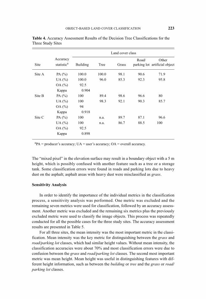
A total of 316, 172, and 208 training samples were used to generate decisiontrees for the three study sites, respectively. The training was successful for all of thethree sites (<1%). Accuracy assessment of the decision tree classifications for thethree sites is presented in Table 4. The decision tree classification for Site A showedgood performance, with an overall accuracy of 92.5% and a Kappa coefficient of0.904. The building and tree categories were well classified, with producer’s anduser’s accuracies over 95%. Some of the other artificial objects were confused withthe grass and road/parking lot objects, yielding lower producer’s accuracy (71.9%).There was also some confusion between the grass and road/parking lot classes.

The classification for Site B produced an overall accuracy of 94% and a Kappa of0.912. There was some confusion between the tree and grass and the tree and otherartificial object classes. Like Site A, the other artificial object class yielded relativelylower accuracies. An overall accuracy of 92.5% and a Kappa 0.898 were achieved forthe classification of Site C. Unlike Sites A and B, the other artificial object categorywas well classified because the class was relatively uniform in shape and size (i.e.,trucks, drum-type storage) and there were no trees on the site.

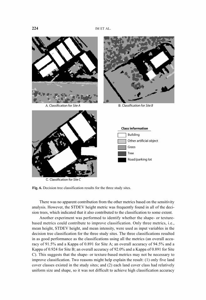
Classified images using decision trees for the three study sites are shown in Fig-ure 6. Based on visual inspection, most of the classification errors were found alongthe boundaries between objects, such as the boundary between a building and road.For example, the height of a building is 10 m and a road next to the building is 0 m.

OBJECT-BASED LAND COVER CLASSIFICATION 223

The “mixed pixel” in the elevation surface may result in a boundary object with a 5 mheight, which is possibly confused with another feature such as a tree or a storagetank. Some classification errors were found in roads and parking lots due to heavydust on the asphalt; asphalt areas with heavy dust were misclassified as grass.

Sensitivity Analysis

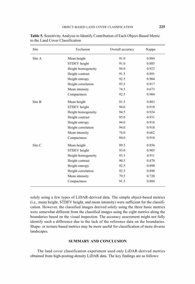
In order to identify the importance of the individual metrics in the classificationprocess, a sensitivity analysis was performed. One metric was excluded and theremaining seven metrics were used for classification, followed by an accuracy assess-ment. Another metric was excluded and the remaining six metrics plus the previouslyexcluded metric were used to classify the image objects. This process was repeatedlyconducted for all the possible cases for the three study sites. The accuracy assessmentresults are presented in Table 5.

For all three sites, the mean intensity was the most important metric in the classi-fication. Mean intensity was the key metric for distinguishing between the grass androad/parking lot classes, which had similar height values. Without mean intensity, theclassification accuracies were about 70% and most classification errors were due toconfusion between the grass and road/parking lot classes. The second most importantmetric was mean height. Mean height was useful in distinguishing features with dif-ferent height information, such as between the building or tree and the grass or road/parking lot classes.

Table 4. Accuracy Assessment Results of the Decision Tree Classifications for the Three Study Sites

SiteAccuracystatistica

Land cover class

Building Tree GrassRoad/

parking lotOther

artificial object

Site A PA (%) 100.0 100.0 98.1 90.6 71.9UA (%) 100.0 96.0 85.3 92.3 95.8OA (%) 92.5Kappa 0.904

Site B PA (%) 100 89.4 98.6 96.6 80UA (%) 100 98.3 92.1 90.3 85.7OA (%) 94Kappa 0.918

Site C PA (%) 100 n.a. 89.7 87.1 96.6UA (%) 100 n.a. 86.7 88.5 100OA (%) 92.5Kappa 0.898

aPA = producer’s accuracy; UA = user’s accuracy; OA = overall accuracy.

224 IM ET AL.

There was no apparent contribution from the other metrics based on the sensitivityanalysis. However, the STDEV height metric was frequently found in all of the deci-sion trees, which indicated that it also contributed to the classification to some extent.

Another experiment was performed to identify whether the shape- or texture-based metrics could contribute to improve classification. Only three metrics, i.e.,mean height, STDEV height, and mean intensity, were used as input variables in thedecision tree classification for the three study sites. The three classifications resultedin as good performance as the classifications using all the metrics (an overall accu-racy of 91.5% and a Kappa of 0.891 for Site A; an overall accuracy of 94.5% and aKappa of 0.924 for Site B; an overall accuracy of 92.0% and a Kappa of 0.891 for SiteC). This suggests that the shape- or texture-based metrics may not be necessary toimprove classification. Two reasons might help explain the result: (1) only five landcover classes existed in the study sites; and (2) each land cover class had relativelyuniform size and shape, so it was not difficult to achieve high classification accuracy

Fig. 6. Decision tree classification results for the three study sites.

OBJECT-BASED LAND COVER CLASSIFICATION 225

solely using a few types of LiDAR-derived data. The simple object-based metrics(i.e., mean height, STDEV height, and mean intensity) were sufficient for the classifi-cation. However, the classified images derived solely using the three basic metricswere somewhat different from the classified images using the eight metrics along theboundaries based on the visual inspection. The accuracy assessment might not fullyidentify such a difference due to the lack of the reference data on the boundaries.Shape- or texture-based metrics may be more useful for classification of more diverselandscapes.

SUMMARY AND CONCLUSION

The land cover classification experiment used only LiDAR-derived metricsobtained from high-posting-density LiDAR data. The key findings are as follows:

Table 5. Sensitivity Analysis to Identify Contribution of Each Object-Based Metricto the Land Cover Classification

Site Exclusion Overall accuracy Kappa

Site A Mean height 91.0 0.884STDEV height 91.0 0.885Height homogeneity 94.0 0.923Height contrast 91.5 0.891Height entropy 92.5 0.904Height correlation 93.5 0.917Mean intensity 74.5 0.673Compactness 92.5 0.904

Site B Mean height 91.5 0.883STDEV height 94.0 0.918Height homogeneity 94.5 0.924Height contrast 95.0 0.931Height entropy 94.0 0.918Height correlation 94.0 0.918Mean intensity 76.0 0.662Compactness 94.0 0.918

Site C Mean height 89.5 0.856STDEV height 93.0 0.905Height homogeneity 93.5 0.911Height contrast 90.5 0.870Height entropy 92.5 0.898Height correlation 92.5 0.898Mean intensity 79.5 0.720Compactness 91.5 0.884

226 IM ET AL.

• High-posting (< 0.5 m)–density LiDAR data has potential for land cover classi-fication without incorporating other remote sensing data such as high-spatial-resolution multispectral imagery. A series of classifications in this study pro-duced high overall accuracies > 90%.

• Object-oriented analysis using a variety of metrics associated with height, intensity, and shape was successful, resulting in high classification accuracy.

• The sensitivity analysis identified that mean intensity was the most important metric for the land cover classification. Mean intensity was the key to differen-tiating between grass and road/parking lot features. Mean height was the sec-ond most important metric. Every land cover class had a unique mean height, except the grass and road/parking lot classes.

• Texture-based metrics did not contribute to improve the classification accuracy. Simple metrics such as mean height, STDEV height, and mean intensity were sufficient for land cover classification in the study. Texture-based metrics might be more useful to classify more complex landscapes.

• Intensity data were critical to the land cover classification. However, it is noted that they were not consistently recorded over the region. Noise due to inconsis-tent data collection can be easily found in Figure 3E. More reliable intensity data collection may improve land cover classification.

Remote sensing technology continues to evolve. LiDAR data collected in con-junction with metric camera multispectral data is now a reality. Such integration willreduce locational and temporal discrepancy problems associated with fusing differentsensor data (e.g., LiDAR + multispectral). Future research will include applications ofthe method to other environments such as vegetation species identification.

REFERENCES

Baatz, M., Benz, U., Dehghani, S., Heynen, M., Höltje, A., Hofmann, P., Lingen-felder, I., Mimler, M., Sohlbach, M., Weber, M., and G. Willhauck, 2004, eCogni-tion User Guide 4, Munich, Germany: Definiens Imaging, Germany.

Baltsavias, E. P., 1999, “Airborne Laser Scanning: Basic Relations and Formulas,”ISPRS Journal of Photogrammetry & Remote Sensing, 54:199–214.

Benz, U., Hofmann, P., Willhauck, G., Lingenfelder, I., and M. Heynen, 2004, “Multi-resolution, Object-Oriented Fuzzy Analysis of Remote Sensing Data for GIS-Ready Information,” ISPRS Journal of Photogrammetry and Remote Sensing,58:239–258.

Boland, J. and 16 co-authors, 2004, “Cameras and Sensing Systems,” in Manual ofPhotogrammetry, 5th ed., McGlone J. C. (Ed.), Bethesda, MD: ASPRS, 629–636.

Bork, E. W. and J. G. Su, 2007, “Integrating LIDAR Data and Multispectral Imageryfor Enhanced Classification of Rangeland Vegetation: A Meta Analysis,” RemoteSensing of Environment, in press.

Brandtberg, T., 2007, “Classifying Individual Tree Species Under Leaf-off and Leaf-on Conditions Using Airborne LiDAR,” ISPRS Journal of Photogrammetry &Remote Sensing, 61:325–340.

OBJECT-BASED LAND COVER CLASSIFICATION 227

Flood, M. and B. Gutelius, 1997, “Commercial Implications of Topographic TerrainMapping Using Scanning Airborne Laser Radar,” Photogrammetric Engineering& Remote Sensing, 63:327.

Franklin, S. E., Maudie, A. J., and M. B. Lavigne, 2001, “Using Spatial Co-occur-rence Texture to Increase Forest Structure and Species Composition Classifica-tion Accuracy,” Photogrammetric Engineering & Remote Sensing, 67(7):849–855.

Garcia-Quijano, M. J., Jensen, J. R., Hodgson, M. E., Hadley, B. C., Gladden, J. B.,and L. A. Lapine, 2007, “Significance of Altitude and Posting-Density onLiDAR-Derived Elevation Accuracy on Hazardous Waste Sites,” Photogrammet-ric Engineering & Remote Sensing, in press.

Haralick, R. M., 1986, “Statistical Image Texture Analysis,” Handbook of PatternRecognition and Image Processing, Young, T. Y. and K. S. Fu (Eds.), New York,NY: Academic Press.

Hill, R. A. and A. G. Thomson, 2005, “Mapping Woodland Species Composition andStructure Using Airborne Spectral and LIDAR Data,” International Journal ofRemote Sensing, 26:3763–3779.

Hodgson, M. E., Jensen, J. R., Raber, G., Tullis, J., Davis, B., Thompson, G., and K.Schuckman, 2005, “An Evaluation of LIDAR-Derived Elevation and TerrainSlope in Leaf-off Conditions,” Photogrammetric Engineering & Remote Sensing,71(7):817–823.

Hodgson, M. E., Jensen, J. R., Tullis, J. A., Riordan, K., and R. Archer, 2003, “Syner-gistic Use of LIDAR and Color Aerial Photography for Mapping Urban ParcelImperviousness,” Photogrammetric Engineering & Remote Sensing, 69(9):973–980.

Huang, X. and J. R. Jensen, 1997, “A Machine-Learning Approach to AutomatedKnowledge-Base Building for Remote Sensing Image Analysis with GIS Data,”Photogrammetric Engineering & Remote Sensing, 63:1185–1194.

Im, J., 2006, A Remote Sensing Change Detection System Based on Neighborhood/Object Correlation Image Analysis, Expert Systems, and an Automated Calibra-tion Model, Ph.D. Dissertation, Department of Geography, University of SouthCarolina.

Im, J. and J. R. Jensen, 2005, “A Change Detection Model Based on NeighborhoodCorrelation Image Analysis and Decision Tree Classification,” Remote Sensingof Environment, 99:326–340.

Im, J., Jensen, J. R., and J. A. Tullis, 2008, “Object-Based Change Detection UsingCorrelation Image Analysis and Image Segmentation,” International Journal ofRemote Sensing, 29(2):399–423.

Jensen, J. R., 2005, Introductory Digital Image Processing—A Remote Sensing Per-spective, Upper Saddle River, NJ: Prentice Hall, 526 p.

Jensen, J. R., 2007, Remote Sensing of the Environment: An Earth Resource Perspec-tive, Upper Saddle River, NJ: Pearson Prentice-Hall, 592 p.

Jensen, J. R. and J. Im, 2007. “Remote Sensing Change Detection in Urban Environ-ments,” in Geo-spatial Technologies in Urban Environments: Policy, Practice,and Pixels, second ed., Jensen, R. R., Gatrell, J. D., and D. McLean (Eds.),Berlin, Germany: Springer-Verlag. pp. 7–32.

228 IM ET AL.

Lee, D. S. and J. Shan, 2003, “Combining LIDAR Elevation Data and IKONOSMultispectral Imagery for Coastal Classification Mapping,” Marine Geodesy,26:117–127.

Leonard, J., 2005, Technical Approach for LIDAR Acquisition and Processing, Fred-erick, MD: EarthData Inc., 20 p.

Mackey, H. E., 1998, Roles of Historical Photography in Waste Site Characterization,Closure, and Remediation, Aiken, SC: Westinghouse Savannah River Company,WSRC-MS-98-00096, 13 p.

Maillard, P., 2003, “Comparing Texture Analysis Methods through Classification,”Photogrammetric Engineering & Remote Sensing, 69(4):357–367.

Mikhail, E. M., Bethel, J. S., and J. C. McGlone, 2001, Introduction to Modern Pho-togrammetry, New York, NY, John Wiley, 479 p.

Quinlan, J. R., 2003, Data Mining Tools See5 and C5.0, St. Ives NSW, Australia:RuleQuest Research, [available online at: http://www.rulequest.com/see5-info.html, accessed July 10, 2007].

Raber, G., Jensen, J. R., Hodgson, M. E., Tullis, J. A., Davis, B. A., and J. Berglund,2007, “Impact of LIDAR Nominal Posting Density on DEM Accuracy and FloodZone Delineation,” Photogrammetric Engineering & Remote Sensing,73(7):793–804.

Rottensteiner, F., Trinder, J., Clode, S., and K. Kubik, 2005, “Using the Dempster-Shafer Method for the Fusion of LIDAR Data and Multi-spectral Images forBuilding Detection,” Information Fusion, 6:283–300.

RuleQuest Research, 2005, C5.0 Release 2.01 (data mining software), St. Ives,Australia: RuleQuest Research.

Song, J. H., Han, S. H., Yu, K., and Y. I. Kim, 2002, “Assessing the Possibility ofLand-Cover Classification Using LIDAR Intensity Data,” paper presented atISPRS Commission III, Symposium, 9–13 September 2002, Graz, Austria.

Suarez, J. C., Ontiveros, C., Smith, S., and S. Snape, 2005, “Use of Airborne LiDARand Aerial Photography in the Estimation of Individual Tree Heights in Forestry,”Computers & Geosciences, 31(2):253–262.

Toyra, J. and A. Pietroniro, 2005, “Toward Operational Monitoring of a NorthernWetland Using Geomatics-based Techniques,” Remote Sensing of Environment,97:174–191.