O. S. Galaktionov, P. D. Anderson*, G. W. M. Peters, H. E ... – 27.10.03/druckhaus köthen O. S....

IPP_ipp1732 – 27.10.03/druckhaus köthen

MIXING AND COMPOUNDING

O. S. Galaktionov, P. D. Anderson*, G. W. M. Peters, H. E. H. Meijer

Materials Technology, Eindhoven University of Technology, Eindhoven, The Netherlands

Analysis and Optimization of Kenics Static Mixers

The mapping approach is applied to study the distributive mix-ing in the, widely industrially used, Kenics static mixer. Theflexibility of the mapping method makes it possible to studyand compare thousands of different mixer layouts and performoptimization with respect to macroscopic homogenization effi-ciency and interface generation. In the paper two different de-signs of the mixer are investigated. The conventional mixerwith sequentially different twisted blades and adesign wherethe twist direction is maintained constant. In both cases theblade twist angle is varied. Recommendations are given in thechoice of the design of the mixer dependent on the desiredstructure of mixing.

1 Kenics Static Mixer: Introduction

1.1 Mixer Geometry

The underlying idea of the Kenics mixer (and all other static-mixers) is to mimic the “Baker’s transformation” [1, 2] by re-peatedly cutting, re-orienting and stacking material to producea multitude of striations. The Kenics static mixer is a typicalin-line mixing device. It consists of a cylindrical pipe with mix-ing elements fixed inside. The mixing elements are formed byhelically twisted rigid plates (usually of the same pitch), eachdividing the pipe into two twisted semicircular ducts. The in-serts are placed tightly one after another so that the leadingedge of the next insert is perpendicular to the trailing edge ofthe previous one. The flow along the pipe is driven by a pres-sure gradient. Although such mixers are also used at moderate(� 102) Reynolds numbers, we consider the most commoncase of Stokes flow of viscous fluids, where the inertial forcescan be neglected. The mixer configuration as used by Avalosseand Crochet [3] is taken as a starting point. The inner diameterof the pipe is 60 mm, the length of the 180�-twisted bladeequals 115 mm, while its thickness (2 mm) is neglected herefor simplicity. (This assumption seems not to cause any notice-able differences in the mixer’s operation, see the results of [3].)Layouts with blades of different twist direction (both left- andright-oriented) will be considered, and we change the totalblade twist angle while keeping the pitch of the blades the sameas in Avalosse and Crochet [3]. Thus, changing the total bladetwist means actually changing the blade length.

Fig. 1 shows three typical examples of mixer configurations.Although the methods used in the current work easily allow forhigher flexibility, we will mostly limit the analysis to mixersthat are spatially periodic with a repeating period sequence ofexactly two blades of the same absolute twist (except in subsec-tion 4.1), but possibly with a different twist direction. The ob-vious reason is that because of the working principle of the Ke-nics mixer, not much improvement can be expected fromsymmetry-breaking measures (that are rather successful in pro-totype mixing flows [4 to 7]), e. g. by combining long and shortblades. Under these limitations two basic types of design exist[8]: a layout with alternating right and left twist direction, re-ferred to as “RL”, and the layout with blades in the same direc-tion of the twist, referred as “RR”. Since it was shown in [9]that the pitch angle has a rather minor effect on mixer perfor-mance, it is fixed in the current work, and the only parameterto change is the total blade twist angle. Throughout this chapterwe will use the “RR” or “RL” notation for the type of geometrytogether with the blade twist angle (in degrees) to specify a par-ticular mixer geometry. Thus, for example RL-180 stands forthe mixer, combining the blades twisted 180� in both direc-tions, Fig. 1A, as analyzed in [3]. Fig. 1B shows the RR-180configuration as was considered by Hobbs and Muzzio [8],while Fig. 1C illustrates the RL-120 geometry, which was sug-gested as more energy efficient in [9].

138 Hanser Publishers, Munich Intern. Polymer Processing XVIII (2003) 2

Fig. 1. Examples of different Kenics designs, A: a “standard” right-left layout with 180° twist of the blades (RL-180); B: right-right layoutwith blades of the same direction of twist (RR-180); C: (RL-120) right-left layout with 120° blade twist

* Mail address: P. D. Anderson, Materials Technology, EindhovenUniversity of Technology, 5600 MB Eindhoven, The Netherlands

© 2

003

Car

l Han

ser

Ver

lag,

Mun

ich,

Ger

man

y

ww

w.k

unst

stof

fe.d

e/IP

P

Not

for

use

in in

tern

et o

r in

tran

et s

ites.

Not

for

elec

tron

ic d

istr

ibut

ion.

1.2 Principle of Kenics Operation

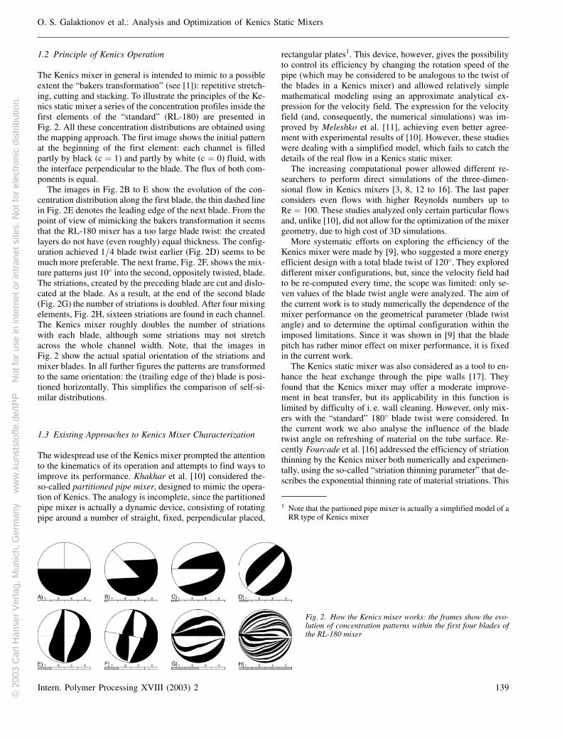
The Kenics mixer in general is intended to mimic to a possibleextent the “bakers transformation” (see [1]): repetitive stretch-ing, cutting and stacking. To illustrate the principles of the Ke-nics static mixer a series of the concentration profiles inside thefirst elements of the “standard” (RL-180) are presented inFig. 2. All these concentration distributions are obtained usingthe mapping approach. The first image shows the initial patternat the beginning of the first element: each channel is filledpartly by black (c ¼ 1) and partly by white (c ¼ 0) fluid, withthe interface perpendicular to the blade. The flux of both com-ponents is equal.

The images in Fig. 2B to E show the evolution of the con-centration distribution along the first blade, the thin dashed linein Fig. 2E denotes the leading edge of the next blade. From thepoint of view of mimicking the bakers transformation it seemsthat the RL-180 mixer has a too large blade twist: the createdlayers do not have (even roughly) equal thickness. The config-uration achieved 1=4 blade twist earlier (Fig. 2D) seems to bemuch more preferable. The next frame, Fig. 2F, shows the mix-ture patterns just 10� into the second, oppositely twisted, blade.The striations, created by the preceding blade are cut and dislo-cated at the blade. As a result, at the end of the second blade(Fig. 2G) the number of striations is doubled. After four mixingelements, Fig. 2H, sixteen striations are found in each channel.The Kenics mixer roughly doubles the number of striationswith each blade, although some striations may not stretchacross the whole channel width. Note, that the images inFig. 2 show the actual spatial orientation of the striations andmixer blades. In all further figures the patterns are transformedto the same orientation: the (trailing edge of the) blade is posi-tioned horizontally. This simplifies the comparison of self-si-milar distributions.

1.3 Existing Approaches to Kenics Mixer Characterization

The widespread use of the Kenics mixer prompted the attentionto the kinematics of its operation and attempts to find ways toimprove its performance. Khakhar et al. [10] considered the-so-called partitioned pipe mixer, designed to mimic the opera-tion of Kenics. The analogy is incomplete, since the partitionedpipe mixer is actually a dynamic device, consisting of rotatingpipe around a number of straight, fixed, perpendicular placed,

rectangular plates1. This device, however, gives the possibilityto control its efficiency by changing the rotation speed of thepipe (which may be considered to be analogous to the twist ofthe blades in a Kenics mixer) and allowed relatively simplemathematical modeling using an approximate analytical ex-pression for the velocity field. The expression for the velocityfield (and, consequently, the numerical simulations) was im-proved by Meleshko et al. [11], achieving even better agree-ment with experimental results of [10]. However, these studieswere dealing with a simplified model, which fails to catch thedetails of the real flow in a Kenics static mixer.

The increasing computational power allowed different re-searchers to perform direct simulations of the three-dimen-sional flow in Kenics mixers [3, 8, 12 to 16]. The last paperconsiders even flows with higher Reynolds numbers up toRe ¼ 100. These studies analyzed only certain particular flowsand, unlike [10], did not allow for the optimization of the mixergeometry, due to high cost of 3D simulations.

More systematic efforts on exploring the efficiency of theKenics mixer were made by [9], who suggested a more energyefficient design with a total blade twist of 120�. They exploreddifferent mixer configurations, but, since the velocity field hadto be re-computed every time, the scope was limited: only se-ven values of the blade twist angle were analyzed. The aim ofthe current work is to study numerically the dependence of themixer performance on the geometrical parameter (blade twistangle) and to determine the optimal configuration within theimposed limitations. Since it was shown in [9] that the bladepitch has rather minor effect on mixer performance, it is fixedin the current work.

The Kenics static mixer was also considered as a tool to en-hance the heat exchange through the pipe walls [17]. Theyfound that the Kenics mixer may offer a moderate improve-ment in heat transfer, but its applicability in this function islimited by difficulty of i. e. wall cleaning. However, only mix-ers with the “standard” 180� blade twist were considered. Inthe current work we also analyse the influence of the bladetwist angle on refreshing of material on the tube surface. Re-cently Fourcade et al. [16] addressed the efficiency of striationthinning by the Kenics mixer both numerically and experimen-tally, using the so-called “striation thinning parameter” that de-scribes the exponential thinning rate of material striations. This


O. S. Galaktionov et al.: Analysis and Optimization of Kenics Static Mixers

Intern. Polymer Processing XVIII (2003) 2 139

Fig. 2. How the Kenics mixer works: the frames show the evo-lution of concentration patterns within the first four blades ofthe RL-180 mixer

1 Note that the partioned pipe mixer is actually a simplified model of aRR type of Kenics mixer

© 2

003

Car

l Han

ser

Ver

lag,

Mun

ich,

Ger

man

y

ww

w.k

unst

stof

fe.d

e/IP

P

Not

for

use

in in

tern

et o

r in

tran

et s

ites.

Not

for

elec

tron

ic d

istr

ibut

ion.



was done by inserting a large number of “feed circles” and nu-merically tracking markers along the mixer. Their method al-lows to characterize the efficiency of the static mixer. However,adjusting the geometry would necessitate repetition of all parti-cle tracking computations. Optimization of the mixer geometrycalls for a special tool that allows to re-use the results of te-dious, extensive computations in order to compare differentmixer layouts. A good candidate for such a tool is the mappingtechnique.

In this work we take into account the most important resultsof [9]. The mapping method is used to systematically study theperformance of Kenics mixers of different geometries (twist di-rection and angle of the blades) and to find its optimal design.

2 Application of the Mapping Technique to the KenicsMixer

2.1 Computational Domain

To implement the mapping approach, the Kenics static mixer issubdivided into independent functional mixing modules. Thesemodules are assembled in an appropriate sequence to obtain thereal mixer design. An essential requirement is that the flow in-side a module can be assumed to be independent on the preced-ing or following ones. The starting point is to select a computa-tional domain that contains all necessary features of the mixer,see Fig. 3A. The direction of the fluid flow is upwards andalthough the configuration is simple, it fulfills our require-ments:� In order to obtain a fully developed flow in the entrance and

exit conditions inflow and outflow sections are providedwith flat blades that subdivide the tube into two straightsemicircular ducts for which an analytical expression,known ina closed form [11], is used to specify the boundaryconditions.

� In its central section the flow domain considered contains along right-twisted blade with total twist angle of 180�. It isassumed (and has yet to be verified) that in the middle zoneof the blade, the velocity field is independent of the axialcoordinate, if viewed in a properly rotated reference frame,aligned with the blade.

� The flat blade in the lower section changes into a right-twisted blade (with total twist of 90�) that forms a R-R tran-sition with the following long right-twisted blade of 180�

twist.� Analogous, in the upper section the 180� right-twisted

blade forms a R-L transition with the following 90� left-twisted blade that smoothly changes into the exit duct.

This configuration contains all necessary elements and there isno need to separately compute a velocity field around a long-left-twisted blade, since it is the mirror image of that of theright-twisted blade. Similarly, the effect of the L-L and L-Rtransition is completely defined by their mirror counterparts(R-R and R-L transitions, respectively).

Fig. 3B shows the surface of the finite element mesh used tocompute the velocity field, containing 13; 824 second-orderhexagonal elements with 116; 145 nodal points (403; 731 de-grees of freedom). At the rigid walls a no-slip boundary condi-tion is prescribed and at both inlet and outlet, a fully developed

Poiseuille profile is prescribed. The fluid is assumed to beNewtonian with a constant viscosity, unless explicitly statedotherwise. Under these conditions the axial velocity in theStokes flow through a vertical semicircular duct x2 þ y2 < a2,y > 0 of the radius a can be expressed by the exact analyticalformula [11]. In polar coordinates ðr; hÞ it reads:

uz ¼2p

p2 � 8huzi

��p

r2

a2sin2 hþ r

a� a

r

� �sin h� 1

4r2

a2� a2

r2

� �sin ð2hÞ

� lnr2 þ 2ar cos hþ a2

r2 � 2ar cos hþ a2

þ 12

2 � r2

a2� a2

r2

� �cosð2hÞ

� �arctan

2ar sin ha2 � r2

�; ð1Þ

where huzi denotes the average axial velocity. A conjugate gra-dient solver, implemented in the SEPRAN finite element pack-age [18] was used to obtain the velocity field inside the mixer.The solution was then exported from SEPRAN and customaryoptimized interpolation routines were used to obtain the veloci-tyin an arbitrary point inside the fluid domain.

140 Intern. Polymer Processing XVIII (2003) 2

Fig. 3. Computing the velocity field patterns in the Kenics, A: the flowdomain; B: the finite element grid; C: the velocities at the cross-sectionin the middle of the long blade; D: the same, but slightly below the R-Ltransition. The contours in (C) and (D) are isolines of the axial velocityuz , the arrows show the lateral velocity components

© 2

003

Car

l Han

ser

Ver

lag,

Mun

ich,

Ger

man

y

ww

w.k

unst

stof

fe.d

e/IP

P

Not

for

use

in in

tern

et o

r in

tran

et s

ites.

Not

for

elec

tron

ic d

istr

ibut

ion.

Two typical examples of the velocity field are given inFigs. 3C, D. In both images, the contours are isolines of the ax-ial velocity uz and the arrows indicate the lateral velocity com-ponents. The upper right image, Fig. 3C shows the velocities inthe mixer cross-section, located in the middle of the long blade.Interesting is that the distribution of the axial velocity is veryclose to the Poiseuille profile for a straight semicircular duct[11]. Close to the end of the blade the picture, however,changes significantly and an example of the velocity fieldslightly below the R-L transition (at the distance that corre-sponds to 5� turn of the blade) is given in Fig. 3D. The vicinityof the next blade, with opposite twist, not only changes the ax-ial velocity profile, that now has four maxima, but also sup-presses the lateral velocity in the zones, where the fluid is ap-proaching the surface of the next blade.

2.2 Mixing Modules

It is necessary to verify our assumption that the mixer can berepresented as a sequence of modules, some describing thetransition regions of blade junctions, others just sections of dif-ferent lengths with undisturbed velocity fields. To find the dis-tance from the transitions where the flow can be regarded asundisturbed, the velocity field was analyzed in more detail,close to and away from R-R and R-L transitions. A rotationaltransformation was applied to bring all cross-sections to thesame orientation and the deviation of the velocity fields fromthe reference velocity field, taken in the middle of long blade,was analyzed. This deviation is defined as

dv ¼

ffiffiffiffiffiffiffiffiffiffiffiffiffiffiffiffiffiffiffiffiffiffiffiffiffiffiffiffiffiffiffiffiffi1N

XN

i¼1

~uui � ~u0u0ij j2

vuut ; ð2Þ

where ~uui and ~u0u0i are the velocities at the same location (point

number i) in the disturbed and undisturbed (at the middle oflong blade) velocity field, on a grid of N ¼ 1600 points, dis-tributed evenly over the cross-section. Its value, scaled withthe average of the absolute value of velocity hvi, is plotted inFig. 4A versus the distance from the middle of the blade, whichfor convenience is transformed into the turn angle of the blade.Based on these estimations the transition zones are defined asspanning the distance corresponding to a 45� turn of the blade.

(The transition zones were even increased in some tests to 60�

in order to minimize errors and to verify the optimization re-sults. These changes did not make a noticeable difference.)Far from the transition zones the velocity field will be copied(with rotational and reflectional transformations) from the re-ference cross-section.

As will be pointed out in subsection 2.3 the flow tubes mustbe traced in order to obtain the mapping matrix coefficients.The contours enclosing the flow tube are represented by poly-gons and are tracked using an adaptive front tracking scheme[19], until they reach the final cross-section. The residencetime for various markers may differ significantly and grows un-bounded for markers adjacent to the walls, which makesstraightforward tracking complicated. However, since it wasfound that regions of back flow are not present in a Kenics mix-er, and thus the axial velocity uz is positive at any point not lo-cated on the solid surface, it is possible to follow the trajectoryof particles by using the axial coordinate, rather than time, forintegrating the equations of motion. Along the path line of aparticle the derivatives of transversal coordinates x and y are:

dxdz

¼ ux

uz;

dydz

¼ uy

uz: ð3Þ

These derivatives behave smoothly inside the computationaldomain and have well-defined limits at the boundaries. Thus,to facilitate the tracking computations, when a marker islocated too close to the boundary (closer than d ¼ 0:0017R,where R is the tube radius), the derivatives (3) are replaced bytheir values at the nearest internal point located in the samecross-section at the distance d from the wall. After these sim-plifications, Eq. 3 are easily integrated numerically over zusing an adaptive Runge-Kutta scheme.

Fig. 4B shows the secondary flow, described by Eq. 3 in themiddle of the long blade, obtained by subtracting the helicalmotion that would be caused by rotation together with theblade. It is clearly seen that the material is being rotated (neces-sarily deforming) in each of the channels. Note that the plottedvectors are not approaching zero values close to the walls, sincethey were re-scaled with uz, which itself approaches zero there.This relative pattern shows that material striations, being cut bythe blade, are transported in opposite directions along theblade: the behaviour clearly recognizable in the experimentalresults of [3].




Fig. 4. Defining the modules for assemblingdifferent mixer configurations, A: findinghow far the disturbances from blade transi-tions reach. B: revealing the secondary flowin undisturbed region. The scaled velocities(3) are shown

© 2

003

Car

l Han

ser

Ver

lag,

Mun

ich,

Ger

man

y

ww

w.k

unst

stof

fe.d

e/IP

P

Not

for

use

in in

tern

et o

r in

tran

et s

ites.

Not

for

elec

tron

ic d

istr

ibut

ion.



2.3 Mapping Matrices

The “mapping” method is proposed based on the original ideasof Spencer and Wiley [20], and the main idea is not to trackeach material volume in the flow domain separately, but to cre-ate a discretized mapping from a reference grid to a deformedgrid. Within the mapping method a flow domain is subdividedinto N non-overlapping sub-domains Xi with boundaries qXi,see the example in Fig. 5. The boundaries qXi of these sub-do-mains are represented by polygons and tracked from z ¼ z0 toz ¼ z0 þ Dz using an adaptive front tracking model [19], and,as a result, deformed polygons are obtained. The area of the in-tersections of the deformed sub-domains with the originalones, determine the elements of the mapping (or distribution)matrix W, where Wij equals the fraction of the deformed sub-domain qXj at time z ¼ z0 þ Dz that is found in the original(z ¼ z0) sub-domain Xi:

Wij ¼ZXjjz¼z0þDz

TXjjz¼z0

dX=

ZXjjz¼z0

dX ð4Þ

and are computed using the polygonal descriptions of the sub-domains. For details on the validation and accuracy of the map-ping method we refer to [21].

The sub-domain grid, used in determining the mapping ma-trices, contains 1:6 � 105 cells and has the same structure asthe coarse grid, shown in Fig. 5. The fact that the grid is struc-tured makes it computationally inexpensive to find in whichcell any specified point is located and what its neighbouringcells are (which is essential for a fast computation of the map-ping matrix).

Fig. 6 shows schematically the parts of mixer, described bythe computed matrices (the modules). The matrices denotedas RR1 and RR2 represent the sections with 45� blade twist(see Fig. 4) of the transition zones around the R-R transition.Similarly, RL1 and RL2 matrices describe the R-L transition.Different matrices representing various amount of twist of thelong R blade were computed, to be precise matrices describing5�; 10�; 15�; . . . ; 90� twist were used. In Fig. 6 the block, repre-sented by the matrix R90 (90� twist of the right-turning blade)is marked. A total blade twist of 90� is the minimum value in

our optimization (entrance and exit transition zones of 45�

each, without an additional module in between). Symmetry(mirroring transformation) is used to obtain the matrices forthe L-L and L-R transitions and for the left-twisted long Lblade.

When the sparse matrix is determined, its storage is con-verted into a more conventional column-oriented physically or-dered packing, similar to what is done in many commercialpackages. Note, that the sparse storage is essential for usingthe mapping approach. For example the full matrix, describinga 90� twist of the long blade, would contain 2:56 � 1010 ele-ments and would require over 200 Gb of storage memory. Atthe same time the flexible storage, used during the computationof the matrix, only requires 14:8 Mb, while the last, more com-pact storage algorithm, reduces this value even further to just11:3 Mb. This makes a simultaneous storage in RAM possible,as well as handling of multiple matrices simultaneously, on amodern PC. Loading of a matrix from the disk file typically re-quires a few seconds.

While the determination of the mapping matrices requiredtakes some effort (up to 20 hours cumulative CPU time), asingle mapping operation requires only a fraction of a secondof CPU time (of the order of 0:1 second on AMD Ath-lontm1:0 GHz). Thus, mapping makes it possible to evaluate alarge number of mixer layouts and to proceed with a large num-ber of blades, while still obtaining the material striations.

3 Macroscopic Homogenization

3.1 Intensity of Segregation

In order to be able to quantitatively compare different mixturesand, thus, to compare the performance of mixers with variouslayout, we use the flux-weighed, slice-averaged, discrete inten-sity of segregation defined in a cross-section, using coarse grainconcentrations ci in the cells:

I ¼ 1�ccð1 � �ccÞ

1F

XN

i¼1

ðci � �ccÞ2 fi;

where �cc ¼ 1F

XN

i¼1

cifi; F ¼XN

i¼1

fi; ð5Þ

where fi is the volumetric flux through the cell number i and Fis the total flux through the mixer. The intensity of segregationis equal to 1 for an unmixed (only white and black cells) distri-bution and falls to I ¼ 0 for a uniform gray pattern.

Note, that this flux-weighed definition (5) of the intensity ofsegregation (as opposed to the area- or volume-weighed defini-tions used in 2D and 3D closed prototype flows in [7, 22]) is


Fig. 5. Computing the mapping matrix coefficient Wij: the initial sub-domain Xj is tracked and the intersection of the deformed X0

j aftertracking with Xi is determined

Fig. 6. Scheme if the “building blocks” of Kenics mixers

© 2

003

Car

l Han

ser

Ver

lag,

Mun

ich,

Ger

man

y

ww

w.k

unst

stof

fe.d

e/IP

P

Not

for

use

in in

tern

et o

r in

tran

et s

ites.

Not

for

elec

tron

ic d

istr

ibut

ion.

much better suited for analyzing continuous mixers, since thereal influence of an unmixed spot on the value of I is propor-tional to the flux, carried through this spot. The results of usingdefinition (5) may be somewhat different from the visual im-pression of the concentration distribution in slices inside themixer, since the unmixed patches near the mixer walls, andespecially in the corners between the blade and the pipe sur-face, are carrying very little flux, as compared to the inner partsof the channels. One should, though, remember that any de-crease in the computed intensity of segregation is caused bytwo factors: first, the actual homogenization due to mixingand, second, numerical diffusion of the mapping method dueto concentration averaging in every sub-domain after eachmapping step. Thus, the absolute value of I is only indicative.However, comparison of the evolution (rate of decrease) ofthe intensity of segregation for similar mixers allows to revealthe configuration that achieves the fastest mixing. This is opti-mization. We will compare the results of mapping with morestandard methods like Poincar�e sections and, moreover, usethe scale of segregation, or, alternatively, the so-called struc-ture radius [15, 23] to evaluate the size of the largest unmixedregions.

Since an ideal mixture is characterized by an intensity ofsegregation equal to zero, the rate of its (typically exponential)decrease essentially characterizes the mixer efficiency. The de-pendence of I on the axial position, represented by the numberof blades, is illustrated for an RL mixer with different bladetwist angle in Fig. 7A. It clearly shows that in most of the casesexponential mixing is indeed realized, but that the slopes, therates of mixing, vary significantly with the total blade twist an-gle. This plot does not actually provide information about themixer energy efficiency, since mixers with a higher total bladetwist (longer blades) also require more energy to operate dueto larger pressure drop required. Nevertheless, the extremelylow decrease rate of the intensity of segregation for e. g. themixer with 270� twist gives a good indication that this config-uration probably has “dead” zones of regular motion, separatedby KAM boundaries [1]. Fluid contained in such zones doesnot mix with the rest of the flow.

Fig. 7B presents the same data as Fig. 7A, but now I isplotted versus the total pressure drop, given in relative units,scaled with the absolute value of pressure drop DP� along oneblade of the “standard” RL-180 mixer. Among the configura-tions presented in both plots of Fig. 7, the mixer with the blade

twist angle equal to 150� achieves the highest mixture homoge-neity at the lowest pressure drop.

A more precise evaluation was performed by investigatingmixer configurations with a blade twist ranging from 90� to360� with a step of 5�. The results are summarized in Fig. 8,where the logarithm of intensity of segregation is plotted as afunction of pressure drop DP (measured in the same units asin Fig. 7B) and the blade twist angle h. This three-dimensionalplot exhibits a distinctive valley, the bottom of which, in the re-gion of the larger pressure drops DP, is located around the valueof blade twist angle h ¼ 140�. The small “ripple” visible alongthe h ¼ 180� is caused by the fact that for the configurationswith larger h, every blade is modeled with the use of more thenthree mapping matrices (as for smaller values), causing a slightincrease in the “numerical diffusion”, introduced by the map-ping computations (more mapping operations mean more per-cell averaging). This, however, does not alter the general trend.Sub-figures a – f of the Fig. 8 illustrate the mixture patterns,created by mixers with different h at roughly the same pressuredrop. For illustration purposes the pressure drop chosen is rela-tively low. The mixer with h ¼ 90� creates noticeable “irregu-larities” in large regions near the tube surface close to theblades. This effect is milder for h ¼ 120� and, for the optimalconfiguration with h ¼ 140�, these badly mixed zones aresmall and packed closely to the channel corners. At this loca-tion their influence on mixer performance is minimal, sincethe flux through these zones is low. The mixer with the tradi-tional value of h ¼ 180� performs well, achieving good distri-butions, but due to increased pressure drop per blade, it is lessenergy-efficient. Finally, it is clear that the poor mixing at high-er h values, around h ¼ 270� (see Fig. 8E), corresponds to sys-tems with large regular, dead, zones. With further increase ofthe blade twist angle, the mixer seems to work again, but thehigh pressure drops required render it inefficient. From Fig. 8it can be concluded that the preferable blade twist angle for aRL Kenics mixer, with the pitch angle considered in this paper(the same as in [3]), operated at close to zero Reynolds number,with Newtonian fluids, should be h ¼ 140�. The more tradi-tional value of the blade twist, h ¼ 180�, corresponds to a sharpslope of the valley in Fig. 8 (line d) and small changes of para-meters can be expected to have a strong influence on its perfor-mance, although not necessarily deteriorating it.

Fig. 9 is similar to Fig. 8 but describes the behaviour of RRmixer. The RR mixer with h ¼ 180� is unable to homogenize




Fig. 7. Dependence ofthe intensity of segrega-tion on number ofblades (A) and onscaled pressure drop(B) for RL mixers withdifferent blade twist an-gle

© 2

003

Car

l Han

ser

Ver

lag,

Mun

ich,

Ger

man

y

ww

w.k

unst

stof

fe.d

e/IP

P

Not

for

use

in in

tern

et o

r in

tran

et s

ites.

Not

for

elec

tron

ic d

istr

ibut

ion.



components because it possesses rather large unmixed islands,which are also present for a wide range of blade twist values.Not all RR configurations of the Kenics mixer are sufferingfrom large “dead” zones, see e. g. the RR-110 configuration,although its efficiency is still noticeably lower than that of theRL-140 mixer.

From a mixing point of view the RR mixer is much less in-teresting than the RL mixer. However, some other interestingapplications come to mind if we examine the RR-180 concen-tration patterns. This typical configuration of the Kenics mixercan be used to create rather specific structures where two poly-mers with different properties are mixed in the core of mixer,

enclosed by two large unmixed regions each con-taining the pure polymer components. Examples ofpossible technological applications are:

(i) controlled curling of fibers, mimicking naturalwool, by using two polymers with different thermalshrinkage, that are, though, closely interconnectedin the middle part, and,

(ii) using a combination of conductive and non-conductive polymers to produce capacitors etc.

3.2 Influence of a Shear-rate Dependent Viscosity

The results, presented in the previous section wereobtained for Stokes flows of a Newtonian fluid. It isof interest to see how the rheological properties ofthe fluid affect the analysis and the optimization re-sults. In Anderson et al. [24] the influence of ashear-rate-dependent viscosity on mixing qualitywas examined in time-periodic cavity flows. For dif-ferent mixing protocols the non-Newtonian beha-viour could lead to both considerably better andworse mixing compared to the Newtonian case. Fanet al. [25] reported similar results for the journalbearing flow. Here, we study the influence of ashear-rate-dependent viscosity on the mixing perfor-mance of Kenics mixers and the viscosity g of thefluid is described by Carreau-Yasuda model withzero infinite-shear viscosity (see e. g. [26]):

g ¼ g0 1 þ k2jII2Dj �n�1

2 ; ð6Þwhere g0 is the viscosity at zero shear rate, jII2Dj isthe second invariant of the rate of deformation ten-sor and k and 0 � n � 1 are parameters of the mod-el. In the examples below, the total volumetric fluxthrough the mixer is kept the same as before, so thatthe average axial velocity huzi ¼ 1. The parameterk is fixed at k ¼ 10, which ensures that we indeedenter the shear thinning region, and the power coef-ficient n is varied. Decreasing the power parametern in Eq. 6 makes the axial flow profile more plug-like, see Fig. 10A. The change of the power para-meter, while maintaining a constant flux, also re-sults in a change of the pressure drop, which is illu-strated in the table in Fig. 10B. Here the pressuredrops corresponding to the first 45� of the bladenext to the RR or RL transition (DPRR and DPRL, re-spectively) and the pressure drop DP90� along the90� twisted piece of long blade, are given. For com-parison, the pressure drop DP� at one blade of theRL-180 mixeris also presented. The changes inpressure drop are relevant, since a constant totalpressure drop is chosen as a criterion in determiningthe optimal blade twist.


(a): 11 × 90°

(b): 9 × 120°

(c): 8 × 140°(f): 3 × 360° (e): 4 × 270°

(a): 16 × 90°

(b): 13 × 110°

(f): 4 × 360° (e): 5 × 270° (d): 8 × 180° (c): 10 × 140°

(d): 6 × 180°

Fig. 8. Optimization of the blade twist angle for RL mixer (Newtonian fluid): loga-rithm of the intensity of segregation is plotted as a function of the blade twist angleand total pressure drop

Fig. 9. Optimization of the blade twist angle for the RR mixer (Newtonian fluid).The scale is the same as in Fig. 8, while the concentration profiles correspond toon average 30 % larger pressure drop then those shown in Fig. 8

© 2

003

Car

l Han

ser

Ver

lag,

Mun

ich,

Ger

man

y

ww

w.k

unst

stof

fe.d

e/IP

P

Not

for

use

in in

tern

et o

r in

tran

et s

ites.

Not

for

elec

tron

ic d

istr

ibut

ion.

Mapping computations, revealing the dependence of the in-tensity of segregation on pressure drop and blade twist angleof the RL mixer, were performed for four different values ofthe power parameter n ¼ 1:0; 0:7; 0:4 and 0:1. The evolutionof the intensity of segregation for some RL mixers is shown inFig. 11 versus the number of blades and versus pressure dropDp respectively. Note that for the large values of the twist anglethe strong shear thinning behaviour can improve the mixer per-formance, while for small twist angles it deteriorates theachieved mixture quality. The results of similar computationsfor different blade twist angles are summarized in the next fig-ure. The left plot in Fig. 12 shows the intensity of segregationversus the blade twist angle h, achieved at cost of apressuredrop DP equivalent to 12 blades of the RL-180 mixer for theparticular fluid, for four values of n. While the fluids withsmaller n require lower pressure drops, the effect of shear thin-ning on the optimal blade twist is rather moderate. Accordingto Fig. 12, shear thinning slightly shifts the optimum towardsa larger blade twist and, in general, somewhat reduces the effi-ciency of the mixer. As an illustration, the concentration pat-terns after 6 blades of the RL-140 mixer for the Newtonianfluid (n ¼ 1) and shear thinning fluid with n ¼ 0:1 are alsoshown in Fig. 12. These cross-sections look remarkably simi-lar, except for larger striation thicknesses near the walls forthe shear thinning fluid. Their influence on the mixture quality(intensity of segregation) is stronger than it seems based on justa comparison of the two slices, since the shear thinning flowwith its more plug-like profile (see Fig. 10A), carries the thick-er near-wall striations with a larger relative flux. [23] per-formed the experiments with different shear-thinning fluids,




n DPRR DP90� DPRL DP�

1.0 0.2488 0.4621 0.2690 1.00000.7 0.1698 0.3216 0.1825 0.68650.4 0.1150 0.2209 0.1227 0.46630.1 0.0759 0.1461 0.0803 0.3068

B)

Fig. 10. The influence of the shear thinning fluid behaviour on the per-formance of the Kenics mixer, (A) axial velocity along the radius, per-pendicular to the blade in the middle cross section of long blade sec-tion; (B) pressure drop in the various sections of the mixer, scaled onthe pressure drop on a single blade of RL-180 mixer with Newtonian(n =1.0) fluid

Fig. 11. Dependence of theintensity of segregation onnumber of blades (A) andon scaled pressure drop (B)for some RL mixers and itsdependence on shear thin-ning behaviour

n = 1.0 n = 0.1

Fig. 12. Dependence of theRL mixer efficiency on theblade twist angle h for dif-ferent shear thinning para-meter n. Intensity of segre-gation is plotted for thepressure drop equal to thatof 12 blades of RL-180 mix-er for the corresponding li-quid. Concentration pro-files are shown for n = 1.0and n =0.1 after 6 blades

© 2

003

Car

l Han

ser

Ver

lag,

Mun

ich,

Ger

man

y

ww

w.k

unst

stof

fe.d

e/IP

P

Not

for

use

in in

tern

et o

r in

tran

et s

ites.

Not

for

elec

tron

ic d

istr

ibut

ion.



and the influence of shear-thinning behaviour on the mixturepatterns (structure radii were compared) also turned to berather minor.

3.3 Alternative Methods and Mixture Quality Measures

One of the classical dynamical tools to analyse chaotic mixingis the Poincar�e map. In Fig. 13 the concentration patterns aftereight blades of RL and RR mixers, with blade twist h ¼ 180�,are compared with the corresponding Poincar�e maps. The regu-lar islands (white regions) revealed by the Poincar�e map(Fig. 13C) for the RR-180 configuration match the unmixed re-gions revealed on the concentration slice (Fig. 13D) obtainedusing the mapping method for the same flow. The Poincar�emap for RL-180 configuration indicates that this system isglobally chaotic, which is in complete agreement with the map-ping results. The lower density of markers in Poincar�e mapsnear the trailing and leading edge of the blades (cross-like pat-terns) is caused by significantly lower axial velocities there.

Until now we only applied the intensity of segregation I as ameasure of the mixing quality. This mixing measure is well sui-ted to compare the rate of mixing processes and the final mix-tures, and it is the obvious tool for optimization strategies, asclearly demonstrated above. However, I does not provide aquantitative measure of the size of unmixed regions in the mix-ture. In particular if we are interested in scale-up of mixing de-vices this becomes important, since, for example, in geometri-cal up-scaling of the Kenics mixer, I will remain the same,while the structure radius will be proportional to the mixer dia-meter. A mixing measure which is related to the structure of themixture and which provides a quantitative measure of the sizeof unmixed regions is the scale of segregation. This mixing

measure is statistical in nature and was originallysuggested by [27]. The definition of the scale of seg-regation is based on the so-called correlation coeffi-cient (normalized correlation function), defined overthe field of concentration cð~xxÞ as [28]:

qð~rrÞ ¼ h½cð~xxÞ � �cc� ½cð~xx þ~rrÞ � �cc�ih½cð~xxÞ � �cc� ½cð~xxÞ � �cc�i ; ð7Þ

where �cc is the average concentration and the angularbrackets denote an averaging over the whole flow

domain, i. e. over all values of ~xx. The scale of segregation, S,is normally used for so-called clumpy mixtures [28], where thecorrelogram is non-negative and equals zero for j~rrj greater thansome value. S is defined as the volume under the correlogram:

Sð~xxÞ ¼Z

qð~rrÞ dS: ð8Þ

A practical way to compute the correlation coefficient, de-scribed by Tucker [28], involves the computation of the powerspectrum of the concentration distribution using fast Fouriertransformations (FFT). In order to do so for the mixture pat-terns obtained in the Kenics mixer, the concentration sliceswere padded by the area of anideal mixture c ¼ �cc to obtain asquare domain and re-discretized using a 1024 � 1024 uniformrectangular grid. Next, the two-dimensional FFT can be ap-plied.

The correlogram obtained after four blades of RL-180 mixer(Fig. 14A), when the lamellar structure is well developed,shows a narrow central maximum and, typical for layered mix-tures, an oscillating behaviour of qðrÞ. The plot is arranged insuch a way that the point r ¼ 0 corresponds to the center ofthe image. Fig. 14B shows the correlogram of the mixture aftereight blades of the RR-180 mixer. The presence of the unmixedislands (and roughly their orientation) is indicated by the widecentral maximum, while other details of the mixture are al-ready lost.

The mixture patterns created by static mixers typically exhi-bit a lamellar (that is ordered – not a clumpy) structure and thecorrelation coefficient is oscillating taking both positive andnegative values. We can extend the definition (8) of the scaleof segregation S for the case under study by computing onlythe integral of the correlation coefficient qð~rrÞ within the centralmaximum. We used the isoline qð~rrÞ ¼ 0:1 as the boundary ofthis maximum to avoid numerical problems (influence of small


Fig. 13. Poincaré maps (A, C) compared with the concentration patterns for corre-sponding flows (B, D). Concentration patterns are shown after eight blades in bothcases

Fig. 14. The correlograms for the mixtures obtained after four blades of RL-180 mixer, (A) and after eight blades of RR-180 mixer (B) and the de-pendence of the scale of segregation on the number of blades for few mixer layouts (C). The white contour on correlograms correspond to q > 0.1.The scale of segregation was computed as an integral of the correlation coefficient within such a zone in the center

RL-180 >RR-180

© 2

003

Car

l Han

ser

Ver

lag,

Mun

ich,

Ger

man

y

ww

w.k

unst

stof

fe.d

e/IP

P

Not

for

use

in in

tern

et o

r in

tran

et s

ites.

Not

for

elec

tron

ic d

istr

ibut

ion.

errors). Fig. 14C shows the dependence of the computed scaleof segregation on the number of blades for a few mixer layouts.It clearly indicates the presence of islands in two mixers withblades twisted in the same direction (RR-140 and RR-180)and in the RL-270 mixer with a large blade twist. The asympto-tic level of the scale of segregation also gives an estimation ofthe size of unmixed zones for the particular mixer geometry.However, this mixture parameter seems not so useful to rankthe globally chaotic flows according to their efficiency.

Another mixing measure for the scale of the unmixed re-gions that is used is the structure radius, defined as the maxi-

mum radius of a circle that can be drawn in a con-centration slice that contains only one, unmixed,fluid component [15, 23]. Fig. 15 gives some exam-ples of the structure radius and shows its evolutionwith the number of blades for a few mixer configura-tions. The markers indicate the situations for whichthe concentration slices (a – e) are shown. The evolu-tion of the structure radius provides some essentialinformation, quickly showing the flows with regularislands: for these flows the structure radius reachessome non-zero constant value. This mixture qualityparameter is also less suitable for comparing the effi-ciency of different mixer configurations, since itonly shows the size of the unmixed patch but notthe flux, carried by it. For example, it overestimatesthe importance of unmixed “corners” in Fig. 15E ob-tained for the RL-140 mixer. These unmixed patchescarry a much smaller flux than the patches of similarsize at any other location will do. Another obviousdisadvantage of this criterium is its computationalcost: to compute the structure radius requires signifi-cantly more CPU time than a single loop over allsub-domains, as it is the case for the intensity of seg-regation. Moreover, the analysis of the less mixedpatterns, with large unmixed patches, requires alarge number of operations, roughly (since the sub-domain grid is not uniform) proportional to thesquare of the structure radius. Nevertheless the struc-

ture radius provides a useful, and physically meaningful, toolthat can be used during scale-up evaluations of different mix-ers. This is illustrated in Fig. 16, which shows the dependenceof the structure radius on the mixer length for two differentmixers: the reference RL-180 configuration and its two timeslarger copy. From these results one can determine, for example,that, in order to achieve the same value 0:1 of the structure ra-dius, an approximately three times larger length (1:5 timesmore blades) of the larger mixer would be required.

4 Near-wall Material Exchange

4.1 Removing Material from the Pipe Surface

A problem that also could occur in Kenics mixer is the forma-tion of a degraded material layer on the pipe surface due to highresidence times. Thus, it is of interest to examine how the mate-rial initially located near the pipe surface is being advected(whether it leaves the near-wall region and in what time). Thestagnation and degradation at the blades is less prominent:these surfaces are interrupted at the trailing edges.

To evaluate the “wall cleaning” performance of Kenics mix-ers, a special initial pattern was used: the marked fluid initiallyoccupies a ring adjacent to the walls (20 cells wide in400 � 400 mapping grid). The initial concentration pattern isshown in Fig. 17A. Fig. 17B, C demonstrate the effect of oneblade of the RL mixers with 90� and 180� blade twist, respec-tively. Basically, in the range explored a larger blade twist in-creases the wall clearing effect of a single blade.

The distribution of the material, originating from the near-wall region in the RL-140 mixer is shown after different num-




Fig. 15. Dependence of the structure radius (scaled with the mixer diameter) on thenumber of blades of various Kenics configurations and examples of the structure ra-dius detection (A to E)

Fig. 16. Scale-up evaluation of the RL-180 mixer: dependence of thestructure radius (scaled with the diameter of the reference mixer) onthe mixer length. The mixer length is scaled with the length of oneblade of the reference mixer

© 2

003

Car

l Han

ser

Ver

lag,

Mun

ich,

Ger

man

y

ww

w.k

unst

stof

fe.d

e/IP

P

Not

for

use

in in

tern

et o

r in

tran

et s

ites.

Not

for

elec

tron

ic d

istr

ibut

ion.



ber of blades in Fig. 18. It is clear that some “old” material isstill on the pipe surface after six blades, and the largest non-cleared areas are near the corners.

The wall-cleaning effect of just two blades is shown inFig. 19 for different blade twist angles from 90� to 210�. Again,we see more efficient cleaning and smaller “corner effects” in

case of large blade twist angles. For mixers with a large bladetwist angle the exchange between the near-wall layer and thebulk of the flow is improved. The estimations can also be per-formed regarding the flux of the marked material still in thewall zone instead of the relative area. The area, however, maybe rather relevant, since the degraded material may solidify onthe wall surface (in that case it is the layer thickness that mat-ters).

The results presented above may indicate that the mixers,achieving fast homogenization (like RL-140 layout consideredearlier) may suffer from material degradation more than mixerswith larger blade twist. A possible solution could be to com-bine short and long blades in the mixer layout, for example in-serting after certain number of short blades a couple of longerones in order to improve clearing of the pipe wall. The mappingmethod allows to explore different mixing layouts where thetwist angles may be adjusted independently. Fig. 20 showstwo examples. The first combines long 180� blades with short-er 120� blades in an alternating pattern 180�=120�=180�=120�.Although the wall cleaning performance of this layout is betterthen that of RL-140 mixer (see Fig. 20B), the homogenizationefficiency is strongly deteriorated: the intensity of segregationdecreases slower then in standard RL-180 case, as it is shownin Fig. 20A. From a number of tests performed it follows thatsimilar configurations that have a two-blade RL repeating se-quence with unequal blade twist angle generally do not mixfast. However, more complex layouts like shown in Fig. 20RL-180/120/120/180 (the same blades in different order) dooffer a compromise between, for example, good homogeniza-tion efficiency of RL-140 layout and wall cleaning features ofsimple RL configurations with longer blades. Depending onthe degree of emphasis laid upon the homogenization effi-ciency and wall cleaning, various Kenics layouts may be se-lected.

5 Residence Time Distribution

Since material degradation due to excessive residence times orstagnation effects is an important issue in static mixers, it isalso of interest to analyse the residence time distribution pat-terns. To include the residence time into the mapping simula-tions, the increment of the residence time caused by differentmixing modules was computed. The interval of time requiredfor the material originating for each donor cell of the mapping


Fig. 17. The clearing of near-wall region by one blade of RL-mixer,(A) initial pattern; (B) RL-90 mixer; (C) “standard” RL-180 mixer

Fig. 18. The clearing of near-wall region by the RL-140 mixer, (A) twoblades; (B) four blades; (C) six blades

A)

E)

Fig. 19. The clearing of near-wall region by two blades of RL mixers,(A) initial pattern; (B) h = 90°; (C) h = 120°; (D) h = 150°; (E)h = 180°; (F) h = 210°

Fig. 20. The dependenceof the intensity of segrega-tion (A) and residue onthe wall (B) on the pres-sure drop for some Kenicsconfigurations. See textfor further explanations

© 2

003

Car

l Han

ser

Ver

lag,

Mun

ich,

Ger

man

y

ww

w.k

unst

stof

fe.d

e/IP

P

Not

for

use

in in

tern

et o

r in

tran

et s

ites.

Not

for

elec

tron

ic d

istr

ibut

ion.

grid to reach the destination cross-section was computed. Thistime was estimated by tracking a single marker, placed initiallyin the centroid of the donor mapping cell. Thus, we imply thatthis time characterizes the whole cell. Note, that the residencetime not always can be averaged over the fluid volume. In par-ticular, the residence time of the material near the rigid wall isunbounded due to non-slip boundary conditions. As a result,the mapping technique that uses volume-averaged coarse grainvalues may underestimate the high values of residence time,caused by stagnation on the rigid walls. It may, nevertheless,produce useful estimations, locating “dangerous” zones. Theresidence time is properly incremented on every step andmapped similarly to the “wall-path”, considered in section 4.

Fig. 21A illustrates the residence time distribution after twoblades of the “standard” RL-140 mixer. The decimal logarithmof the relative residence time t=t� is shown. The scaling factoris the “characteristic time” t� ¼ Dz=hvzi during which the par-ticle that moves with average axial velocity hvzi would travelthe length Dz of the mixer being analysed. The black contoursin Fig. 21A separate the areas where the relative residence timeis larger and smaller then its average value (one – according todefinition). As expected, high residence times are observednear the walls, especially in the corner regions. The additionalcurved strip of material with high residence time, which isvisible in both channels, is the trail of the previous blade.

Fig. 21B, C show the distribution of the relative residencetime after 14 blades of RL-180 and after 18 blades of RL-140mixers, respectively. These mixer layouts with the given num-ber of blades have equal total length and, consequently, equal

characteristic times. Both plots use exactly the same grayscale-map. The maximum residence times observed in the mix-er with the smaller blade twist are somewhat larger then in thestandard configuration. In both cases old material is concen-trated near the corners of the channels. For the RL-140 mixer,however, the zones with old material are reaching further awayfrom the blade. These results are in the qualitative agreementwith the estimates obtained in section 4. Since the materialwith high residence times is found in the corner regions, wherethe velocities are low, its contribution to the total flux is ratherlow. If the cumulative flux of the material with a residence timelower then certain threshold is plotted as a function of this(threshold) residence time, see Fig. 22, it turns that theRL-140 mixer exhibits an even more step-like profile, as com-pared to the standard RL-180 configuration.

6 Discussion and Conclusions

The flow in the Kenics static mixer was studied and the depen-dence of the mixing efficiency on the most relevant geometri-cal parameter – the blade twist angle – was investigated. Thepitch of the blades was kept constant (as in [3]) and the mixerconfigurations with alternating and with the same direction ofblade twist were considered. The velocity field was computedusing a finite element method. To enable efficient modeling ofvarious mixer configurations, the evolution of concentrationpatterns was simulated using the mapping method.

Hobbs and Muzzio [9] studied the performance of the RLKenics mixer for different blade twists but, since they had to re-compute the velocity field every time, only a limited number ofh values could be considered (h ¼ 30� step 30� until 210�).Using the stretching efficiency as acriterion, they concludedthat a 120� blade twist results in the most energy efficient mix-er with respect to the pressure drop required. In the currentwork the possibility to quickly analyze a wide range of twistangles with smaller increments (Dh ¼ 5�) yielded a distinct op-timal twist angle equal to h ¼ 140�. The criterion used to findthis optimum (the volume-flux weighed, slice-averaged, dis-crete intensity of segregation) seems preferable (and of moredirect nature) above the one used by [9]. Moreover, the map-ping method reveals the distinct material striations at more ad-vanced mixing stages then it is typically achievable with mar-ker tracking [3, 8, 9].

Shear thinning behaviour of the fluid viscosity has only asurprisingly small effect on the concentration patterns, pro-duced by the Kenics mixer, confirming the partial results of[3]. It causes a slight increase of the optimal angle and resultsin a somewhat lower efficiency of the mixer. The visible effectis the increasing thickness of the near-wall material striations.In general, it appears that we can expect shear thinning to havea rather moderate effect on mixing behaviour in static mixers(pressure-driven flows). In drag-driven time-periodic cavityflows [24] a more significant effect of shear thinning on flowperformance was observed.

The Kenics mixer with all blades twisted in the same direc-tion (RR) is known to be not efficient, leaving large unmixedstreaks [9]. However, it was found that in a certain range oftwist angles it can also achieve global mixing, although themixing efficiency is still noticeably lower then for the mixer




Fig. 21. The relative residence time log10(t /t*) after 2 blades (A) and14 blades (B) respectively of RL-180 mixer and after 18 blades ofRL-140 (C). See text for further explanations

Fig. 22. The cumulative fraction of the flux of material with relativeresidence time below certain threshold is plotted as a function of thethreshold value. These plots correspond to the residence time distribu-tions shown in Fig. 21B, C

© 2

003

Car

l Han

ser

Ver

lag,

Mun

ich,

Ger

man

y

ww

w.k

unst

stof

fe.d

e/IP

P

Not

for

use

in in

tern

et o

r in

tran

et s

ites.

Not

for

elec

tron

ic d

istr

ibut

ion.



with an alternating direction of the blade twist. The computedoptimal twist angle for the RR mixer was close to h ¼ 110�.The remarkable concentration patterns, created by the RR Ke-nics mixer in the middle range of twist angles, with two well-defined unmixed islands separated by exponentially mixedstriations in between (Fig. 9C, D) could have some interestingtechnological applications, other than creating a perfect mix-ture. The size of the unmixed regions is easily controlled bythe blade twist angle.

The scale of segregation can be used to determine the sizeand shape of the largest unmixed regions. Its asymptotic levelprovides an estimation of the size of the unmixed zones forthe particular mixer geometry, while the shape of the centralmaximum on the correlogram indicates their orientation. Analternative mixing measure that is used in literature is the struc-ture radius, which has a simple geometrical meaning and ismore “intuitive”. It demonstrates the same trends as found be-fore with the use of the intensity of segregation, but it requiresmore extensive computations for its evaluation. From theseanalyses of a rather traditional mixer, as the Kenics static mixerwith its rather simple geometry, it can be concluded that themapping method, combined with proper mixing quality mea-sures, provides a powerful design tool in optimizing mixersfor their performance.

References

1 Ottino, J. M.: The kinematics of mixing: stretching, chaos andtransport. Cambridge texts in applied mathematics. Cambridge Uni-versity Press (1989)

2 Fox, R. F.: Chaos 8, p. 462 (1998)3 Avalosse, Th., Crochet, M. J.: AIChE J. 43, p. 588 (1997)4 Franjione, J. G., Leong, C.-W., Ottino, J. M.: Phys. Fluids. A, 1,

p. 1772 (1989)5 Liu, M., Peskin, R. L., Muzzio, F. J., Leong, C. W.: AIChE J. 40,

p. 1273 (1994)6 Anderson, P. D., Galaktionov, O. S., Peters, G. W. M., v. d. Vos-

se, F. N., Meijer, H. E. H.: J. Fluid Mech. 386, p. 149 (1999)

7 Galaktionov, O. S., Anderson, P. D., Kruijt, P. G. M., Pe-ters, G. W. M., Meijer, H. E. H.: Comput. Fluids 30, p. 271 (2001)

8 Hobbs, D. M., Muzzio, F. J.: Phys. Fluids 10, p. 1942 (1998)9 Hobbs, D. M., Muzzio, F. J.: Chem. Eng. Sci. 53, p. 3199 (1998)

10 Khakhar, D. V., Franjione, J. G., Ottino, J. M.: Chem. Eng. Sci. 42,p. 2909 (1987)

11 Meleshko, V. V., Galaktionov, O. S., Peters, G. W. M., Meijer,H. E. H.: Eur. J. Mech./Part B – Fluids 18, p. 783 (1999)

12 Hobbs, D. M., Muzzio, F. J.: Chem. Eng. J. 67, p. 153 (1997)13 Hobbs, D. M., Swanson, P. D., Muzzio, F. J.: Chem. Eng. Sci. 53,

p. 1565 (1998)14 Hobbs, D. M., Muzzio, F. J.: Chem. Eng. J. 70, p. 1942 (1998)15 Byrde, O., Sawley, M. L.: Comput. Fluids 28, p. 1 (1999)16 Fourcade, E., Wadley, R., Hoefsloot, H. C. J., Green, A., Iedema, P. D.:

CFD calculation of laminar striation thinning in static mixer reac-tors. Chem. Eng. Sci. 56, p. 6729 (2001)

17 Joshi, P., Nigam, K. D. P., Nauman, E. B.: Chem. Eng. J. 59, p. 265(1995)

18 Segal, A.: SEPRAN, user manual, standard problems and program-ming guide. Ingenieursbureau SEPRA, Leidschendam (1984)

19 Galaktionov, O. S., Anderson, P. D., Peters, G. W. M., v. d. Vos-se, F. N.: Int. J. Numer. Meth. Fluids 32, p. 201 (2000)

20 Spencer, R. S., Wiley, R. H.: J. Colloid Sci. 6, p. 133 (1951)21 Kruijt, P. G. M., Galaktionov, O. S., Anderson, P. D., Pe-

ters, G. W. M., Meijer, H. E. H.: Mapping method for mixing opti-mization, in: Heino Thiele (Ed.), VDI-K Jahrestagung, Proceeding,p. 3. VDI Verlag, Düsseldorf (2000)

22 Kruijt, P. G. M., Galaktionov, O. S., Anderson, P. D., Pe-ters, G. W. M., Meijer, H. E. H.: AIChE J. 47, p. 1005 (2001)

23 Liu, S.: Master’s thesis, McMaster University, Department of Che-mical Engineering, Hamilton, Ontario (2000)

24 Anderson, P. D., Galaktionov, O. S., Peters, G. W. M., v. d. Vos-se, F. N., Meijer, H.E.H.: J. Non-Newtonian Fluid Mech. 93, p. 265(2000)

25 Fan, Y., Tanner, R., Phan-thien, N.: J. Fluid Mech. 412, p. 197(2000)

26 Macosko, C. W.: Rheology: Principles, Measurements and Applica-tions. VCH Publishers, Weinheim (1994)

27 Danckwerts, P. V.: Appl. Sci. Res. A 3, p. 279 (1953)28 Tucker III, C. L.: Principles of Mixing Measurements, in: Mixing in

Polymer Processing. Rauwendaal, C., Marcel Dekker, New York(1991)

Date received: February 3, 2003Date accepted: February 8, 2003


© 2

003

Car

l Han

ser

Ver

lag,

Mun

ich,

Ger

man

y

ww

w.k

unst

stof

fe.d

e/IP

P

Not

for

use

in in

tern

et o

r in

tran

et s

ites.

Not

for

elec

tron

ic d

istr

ibut

ion.

O. S. Galaktionov, P. D. Anderson*, G. W. M. Peters, H. E ... – 27.10.03/druckhaus köthen O. S....

Documents

Transcript of O. S. Galaktionov, P. D. Anderson*, G. W. M. Peters, H. E ... – 27.10.03/druckhaus köthen O. S....