O N EXTENSIBLE AND OBJECT RELATIONAL … · volve complex models and analysis methods in...

Linköping Studies in Science and TechnologyDissertation No. 452

O

N

EXTENSIBLE

AND

OBJECT

-

RELATIONAL

DATABASE

TECHNOLOGY

FOR

FINITE

ELEMENT

ANALYSIS

APPLICATIONS

K

JELL

O

RSBORN

Department of Computer and Information ScienceLinköping University, Linköping, Sweden

Linköping 1996

Linköping Studies in Science and TechnologyDissertation No. 452

O

N

EXTENSIBLE

AND

OBJECT

-

RELATIONAL

DATABASE

TECHNOLOGY

FOR

FINITE

ELEMENT

ANALYSIS

APPLICATIONS

K

JELL

O

RSBORN

Department of Computer and Information ScienceLinköping University, S-581 83 Linköping, Sweden

Linköping 1996

Cover illustration: “Color Slices” – from the Chromo Cube series – BECK & JUNG, 1996. Used by permission of BECK & JUNG, Lund, Sweden.

ISBN 91-7871-827-9ISSN 0345-7524

Printed in Sweden by triva-tryck ab, Linköping 1996.

v

PREFACE

The research presented in this thesis has been carried out at the Laboratory for Engi-neering Databases and Systems, Department of Computer and Information Science,Linköping University. It has been financially supported by the Swedish National Boardfor Industrial and Technical Development.

I would like to take this occasion to express my appreciation to my supervisor ProfessorTore Risch for giving me the opportunity to carry out this research, and for his inspiringand excellent supervision during this work. Likewise, the additional supervision and en-couragement from Associate Professor Bo Torstenfelt have been of invaluable impor-tance. I would further like to direct my appreciation to Professor Sture Hägglund for hisencouraging guidance during my research and to Associate Professor Anders Törne forhis support during the initiation of this work. Furthermore, the generosity among mycolleagues to share their knowledge and experiences, have greatly facilitated this work.

I would also like to acknowledge the artists

BECK & JUNG

for their kind generosity ingiving me the permission to use one of their computer artwork in this thesis.

Linköping, August, 1996.

Kjell Orsborn

vii

ABSTRACT

Future

database technology

must be able to meet the requirements of scientific and en-gineering applications. Efficient data management is becoming a strategic issue in bothindustrial and research activities. Compared to traditional administrative database ap-plications, emerging scientific and engineering database applications usually involvemodels of higher complexity that call for extensions of existing database technology.The present thesis investigates the potential benefits of, and the requirements on,

com-putational database technology

, i.e. database technology to support applications that in-volve complex models and analysis methods in combination with high requirements oncomputational efficiency.

More specifically, database technology is used to model

finite element analysis (FEA)

within the field of

computational mechanics

. FEA is a general numerical method forsolving partial differential equations and is a demanding representative for these newdatabase applications that usually involve a high volume of complex data exposed tocomplex algorithms that require high execution efficiency. Furthermore, we work with

extensible

and

object-relational (OR)

database technology. OR database technology isan integration of

object-oriented (OO)

and

relational

database technology that com-bines OO modelling capabilities with extensible query language facilities. The term ORpresumes the existence of an

OR query language

, i.e. a relationally complete query lan-guage with OO capabilities. Furthermore, it is expected that the

database managementsystem (DBMS)

can treat extensibility at both the query and storage management level.

viii

The extensible technology allows the design of

domain models

, that is database repre-sentations of concepts, relationships, and operators extracted from the application do-main. Furthermore, the extensible storage manager allows efficient implementation ofFEA-specific data structures (e.g. matrix packages), within the DBMS itself that can bemade transparently available in the query language.

The discussions in the thesis are based on an initial implementation of a system calledFEAMOS, which is an integration of a

main-memory resident

OR DBMS, AMOS, andan existing FEA program, TRINITAS. The FEAMOS architecture is presented wherethe FEA application is equipped with a local embedded DBMS linked together with theapplication. By this approach the application internally gains access to general databasecapabilities, tightly coupled to the application itself, that include a storage manager, adata model, a database language and processor, transactions, and remote access to datasources. On the external level, this approach supports concurrency, inter-operability,data exchange and transformation, data and operator sharing, data distribution, etc.,among subsystems in an

engineering information system

environment. In the FEAMOSsystem, data representations and their related operators in TRINITAS have piece bypiece been replaced by corresponding representations in AMOS. To be able to expressmatrix operations efficiently, AMOS has been extended with data representations andoperations for numerical linear matrix algebra that handles overloaded and multi-direc-tional foreign functions.

Performance measures and comparisons between the original TRINITAS system andthe integrated FEAMOS system show that the integrated system can provide competi-tive performance. The added DBMS functionality can be supplied without any majorperformance loss. In fact, for certain conditions the integrated system outperforms theoriginal system and in general the DBMS provides better scaling performance. It is theauthors opinion that the suggested approach can provide a competitive alternative fordeveloping future FEA applications.

ix

CONTENTS

1 INTRODUCTION .......................................................................................1

1.1 DATABASE TECHNOLOGY FOR FINITE ELEMENT ANALYSIS. . . . . . 2

1.2 RESEARCH METHOD . . . . . . . . . . . . . . . . . . . . . . . . . . . . . . . . . . . . . . . . . . 6

1.3 RESEARCH SCOPE. . . . . . . . . . . . . . . . . . . . . . . . . . . . . . . . . . . . . . . . . . . . . 6

1.4 THESIS OUTLINE . . . . . . . . . . . . . . . . . . . . . . . . . . . . . . . . . . . . . . . . . . . . . . 7

1.5 NOTATIONS . . . . . . . . . . . . . . . . . . . . . . . . . . . . . . . . . . . . . . . . . . . . . . . . . . 8

2 FINITE ELEMENT ANALYSIS AND SOFTWARE .............................9

2.1 FINITE ELEMENT ANALYSIS . . . . . . . . . . . . . . . . . . . . . . . . . . . . . . . . . . . 9

2.2 THE FINITE ELEMENT ANALYSIS PROCESS . . . . . . . . . . . . . . . . . . . . . 11

2.3 FINITE ELEMENT ANALYSIS CONCEPTS. . . . . . . . . . . . . . . . . . . . . . . . 13

2.4 SOFTWARE FOR FINITE ELEMENT ANALYSIS. . . . . . . . . . . . . . . . . . . 22

x

2.5 THE TRINITAS SOFTWARE . . . . . . . . . . . . . . . . . . . . . . . . . . . . . . . . . . . . 25

3 DATABASES AND DATABASE MANAGEMENT SYSTEMS..........29

3.1 CHARACTERISTICS AND OBJECTIVES OF DATABASE SYSTEMS . . 32

3.2 CONVENTIONAL DATABASE TECHNOLOGY . . . . . . . . . . . . . . . . . . . . 34

3.2.1 Hierarchical database management systems . . . . . . . . . . . . . . .34

3.2.2 Network database management systems . . . . . . . . . . . . . . . . .35

3.2.3 Relational database management systems . . . . . . . . . . . . . . . .35

3.3 OBJECT DATABASE TECHNOLOGY . . . . . . . . . . . . . . . . . . . . . . . . . . . . 36

3.3.1 Object-oriented concepts . . . . . . . . . . . . . . . . . . . . . . . . .36

3.3.2 Object-oriented and object-relational database technology . . . . . . .38

3.4 EXTENSIBLE DATABASE TECHNOLOGY . . . . . . . . . . . . . . . . . . . . . . . 40

3.5 MAIN-MEMORY DATABASE TECHNOLOGY. . . . . . . . . . . . . . . . . . . . . 42

3.6 ADDITIONAL DATABASE TECHNOLOGIES. . . . . . . . . . . . . . . . . . . . . . 43

3.6.1 Distributed database management systems . . . . . . . . . . . . . . .43

3.6.2 Active database management systems . . . . . . . . . . . . . . . . . .44

3.7 SCIENTIFIC AND ENGINEERING DATABASE TECHNOLOGY . . . . . . 45

3.8 QUERY LANGUAGES FOR DBMS. . . . . . . . . . . . . . . . . . . . . . . . . . . . . . . 52

3.8.1 Relational algebra and relational calculus . . . . . . . . . . . . . . . .53

3.8.2 The SQL language . . . . . . . . . . . . . . . . . . . . . . . . . . . .55

3.8.3 Object-oriented query languages . . . . . . . . . . . . . . . . . . . . .56

4 THE AMOS DBMS AND THE AMOSQL LANGUAGE .....................59

4.1 THE MEDIATOR APPROACH . . . . . . . . . . . . . . . . . . . . . . . . . . . . . . . . . . . 60

4.2 THE AMOS ARCHITECTURE . . . . . . . . . . . . . . . . . . . . . . . . . . . . . . . . . . . 63

xi

4.3 THE AMOSQL LANGUAGE . . . . . . . . . . . . . . . . . . . . . . . . . . . . . . . . . . . . 67

4.3.1 Objects, types, and functions. . . . . . . . . . . . . . . . . . . . . . .67

4.3.2 AMOSQL data management . . . . . . . . . . . . . . . . . . . . . . .70

4.4 EMBEDDING, INTERFACING AND EXTENDING AMOS . . . . . . . . . . . 72

5 THE FEAMOS APPROACH...................................................................77

5.1 THE FEAMOS ARCHITECTURE. . . . . . . . . . . . . . . . . . . . . . . . . . . . . . . . . 79

5.2 EXTENDING AMOS WITH LINEAR MATRIX ALGEBRA . . . . . . . . . . . 83

5.2.1 Linear algebra for finite element analysis . . . . . . . . . . . . . . . .84

5.2.2 Matrix algebraic concepts . . . . . . . . . . . . . . . . . . . . . . . .86

5.2.3 The matrix foreign data source. . . . . . . . . . . . . . . . . . . . . .96

5.2.4 The array foreign data source . . . . . . . . . . . . . . . . . . . . . 108

5.3 FINITE ELEMENT ANALYSIS DOMAIN MODELLING . . . . . . . . . . . . 112

5.3.1 Geometry and topology . . . . . . . . . . . . . . . . . . . . . . . . 113

5.3.2 The discretisation process . . . . . . . . . . . . . . . . . . . . . . . 129

5.3.3 Finite element analysis solution algorithms . . . . . . . . . . . . . . 138

5.3.4 Result evaluation . . . . . . . . . . . . . . . . . . . . . . . . . . . . 143

5.4 PERFORMANCE ISSUES . . . . . . . . . . . . . . . . . . . . . . . . . . . . . . . . . . . . . . 148

6 RELATED TECHNOLOGIES ..............................................................157

6.1 IMPLEMENTATION TECHNOLOGIES . . . . . . . . . . . . . . . . . . . . . . . . . . 157

6.2 THE STEP STANDARD AND THE EXPRESS LANGUAGE. . . . . . . . . . 159

7 SUMMARY..............................................................................................161

7.1 CONCLUSIONS . . . . . . . . . . . . . . . . . . . . . . . . . . . . . . . . . . . . . . . . . . . . . . 161

7.2 FUTURE WORK . . . . . . . . . . . . . . . . . . . . . . . . . . . . . . . . . . . . . . . . . . . . . 164

xii

8 REFERENCES ........................................................................................167

APPENDIX A: TRINITAS CONCEPTS. . . . . . . . . . . . . . . . . . . . . . . . .179

APPENDIX B: FEAMOS DOMAIN MODEL . . . . . . . . . . . . . . . . . . . .183

APPENDIX C: FEAMOS FOREIGN FUNCTIONS . . . . . . . . . . . . . . .189

1

1 INTRODUCTION

Future

database management systems (DBMSs)

must be able to meet the requirementsof scientific and engineering applications. Scientific and engineering data managementis becoming a strategic issue in both industrial and scientific communities. A high lev-erage is confined in providing efficient information management and flexible informa-tion systems in enterprises as well as for research. In the engineering field, an

engineer-ing information system (EIS)

is responsible for providing information among severalengineering and business disciplines, as indicated in Figure 1, to support the completeproduct life-cycle of various products. Most simplified, the scientific field commonlyhas the problem of handling large amounts of empirical data sets provided by some testequipment on ground or in space. It is believed that database technology can play a sim-ilar and important role in the implementation of scientific and engineering applicationsof tomorrow, as it is currently doing in administrative applications.

In contrast to traditional administrative database applications, applications in scienceand engineering usually involve more complex models that need to be represented inthe database. This calls for extensions of existing database technology to be able to han-dle these models efficiently [1] [2] [3].

Furthermore, there are activities concerned with various types of advanced analyses thatinclude computational intensive tasks and form a subset of all activities that should besupported in a scientific or engineering information system. This can include severalkinds of mechanical, electrical, chemical analyses, etc. These kinds of activities are also

2

found in other fields such as in advanced financial and statistical applications. In addi-tion to models of higher complexity, these activities include computational-intensiveand complex analysis methods. Together, this requires that extensions of existing data-base technology should support data and operator representation capabilities that pre-serve efficient data processing. We use the term

computational database technology

torefer to database technology that should support applications emphasising processingefficiency and needs for complex and application-specific operations. It is intended thatthis should be a unifying term for database technology, in engineering, science, statis-tics, etc., that emphasise the computational aspect in addition to more conventional datamanagement.

Figure 1.

Engineering information management should support several disciplines in an engineering information system environment.

1.1 DATABASE TECHNOLOGY FOR FINITE ELEMENT ANALYSIS

The present thesis focuses on database technology for applications within the computa-tional mechanics field. The potential benefits of, and the requirements on, databasetechnology for supporting these applications are investigated. More specifically, ourwork is on the

next generation extensible and object-oriented (OO) database technolo-gy

, also referred to as


database technology,

DBMS

[4], Frank [5],and Stonebraker and Moore [6]. OR database technology is an integration of OO andrelational database technology that combine OO modelling capabilities with query lan-guage facilities. Hence, OR presumes the existence of a

relationally complete

OO query

EIS

AnalysisDesign

Marketing

ManufacturingMaintenance

Testing

Finance

Recycling

3

language

. Further it is expected that the DBMS can treat extensibility at both the queryand storage management level. We use DBMS technology to model the field of

finiteelement analysis (FEA)

, a general numerical method for solving partial differentialequations. FEA is a demanding representative of these new database applications thatusually involve a high level of complexity of both data and algorithms, as well as a highvolume of data and high requirements on execution efficiency. The discussions in thethesis are based on an initial implementation of a system called FEAMOS [7], which isan integration of a

main-memory (MM) resident

OR DBMS, AMOS [8] [9], and an ex-isting FEA program, TRINITAS [10] [11].

The AMOS design intends to provide a lightweight and open DBMS architecture thatshould permit an easy combination and integration with other applications. It shouldfurther facilitate tailoring and extension of the DBMS to suit the needs of demandingapplications as found in the engineering area. AMOS is intended to perform as a medi-ating software layer, [12]

[13]

[14], among applications and data sources for locating,storing, retrieving, exchanging, transforming, and monitoring data. AMOS can be anembedded database within an application by directly linking AMOS to the applicationat compile time. The application and the DBMS will then be executing in the same com-puter process and be sharing its address space. In addition, AMOS can be used in a con-ventional client-server environment where the applications and the DBMS have theirown computer processes via the client-server interface. It is also possible to define do-main-specific packages of specialised data structures and operators, and integrate themwith AMOS. AMOS has the ability to seamlessly define and call foreign functions (im-plemented in C or LISP) through its foreign data source interface.

AMOS further includes the AMOSQL query language that, in this work, has been usedto represent and manipulate the

domain conceptualisation

, i.e. concepts, relationships,and operations, of the FEA domain. AMOSQL is a more than relationally complete andextensible OO query language that is an extended derivative of OSQL, Lyngbaek [15].The query language is influenced and has much in common with new standardisationefforts for query languages like SQL3, Melton [16], and OQL, Cattell [17].

TRINITAS is a general-purpose FEA program that integrates the entire analysis processand that can be completely controlled through a graphical user interface, illustrated inFigure 2. A typical TRINITAS session includes an interactive problem specification interms of geometry, boundary conditions and domain properties. This is followed by adiscretisation phase, a solution phase, and an evaluation of the results of the calculation.The TRINITAS system currently includes functionality for analysing static, dynamic,and eigenvalue problems within the mechanical design domain, including elastic andthermal effects. In addition, TRINITAS includes capabilities to handle adaptivity, opti-mization, and contact problems in static cases. The TRINITAS program does not incor-porate any data or result files. Instead, all model interaction is performed through thegraphical user interface that accesses main-memory data structures representing theanalysis model. It is further designed in a highly structured, “object-based”, mannerwith specific sets of procedures for each concept, such as point or line.

4

In FEAMOS, both structure and process of the FEA domain are modelled in the data-base

.

This is done by defining a

domain model

using the extensible OR query language,the extensible query optimizer, and the extensible storage manager. A domain modelrepresents a specific category of the mediator layers that are responsible for managingapplication-specific knowledge. The domain model is a database representation of con-cepts, relationships, and operators extracted from the application domain. In our case, adatabase schema is defined to represent finite element (FE) methodology, i.e. FE mod-els and solution algorithms. The extensible query language allows domain-specific FEoperators to be included in the DBMS. A user can define queries in terms of the FEmodel, and the queries may contain FE specific operators. By providing cost hints tothe extensible query optimizer the execution cost of new operators in the query lan-guage can be treated by the optimizer. Furthermore, the extensible storage manager al-lows efficient implementation of FEA-specific data structures (e.g. matrix packages)within the DBMS itself and then made transparently available in the query language.

Figure 2.

A “FEA model”, analysed in the FEAMOS system, shows a view of the graphical user interface of TRINITAS.

The thesis presents an architecture for the integrated FEAMOS system where the FEAapplication is equipped with a local embedded MM DBMS that is linked into the appli-

5

cation [18]. By this approach the application gains access to general database capabili-ties tightly coupled to the application itself, providing a storage manager, data model,database schema, database language and processor, transaction processing, and remoteaccess to data sources. On the external level, this approach supports, for example, con-currency, inter-operability, data exchange and transformation, data and operator shar-ing, data distribution among applications and data sources in the engineering informa-tion system (EIS) environment. Different AMOS mediators are here responsible for lo-cating, translating, and integrating data in various data sources for the applications.Ultimately, the DBMS can decide how and where to execute a query, using query opti-mization techniques. Internally, the architecture provides the application with powerfuland high-level modelling capabilities through the object-relational query language.This includes object identities, subtyping, inheritance, views, overloaded functions,multi-directional functions, and foreign functions. The modelling capabilities make itpossible to design database schemas that possess both physical and logical data and op-erator independence. Hence, the query language modelling supports and facilitateshigh-level application modelling that increases flexibility, composability, and reusabil-ity of domain conceptualisations.

It is of vital importance for the application to preserve the execution efficiency whileadding functionality to the system. The present approach supports this requirement inseveral ways. Most important is the ability to provide an embedded database where theapplication can access and update data through a fast-path interface using precompiledand preoptimized database functions. The AMOS extensibility with foreign data sourc-es, i.e. packages of specialised data representations and operations, makes it possible toprovide efficiency for critical activities. For instance, scientific and engineering appli-cations usually involve large amounts of numerical data that must be represented andprocessed effectively. By providing specialised representations and operations it is pos-sible to avoid unnecessary copying and transformation of data. Execution efficiency isalso supported by the query processor that has the ability to optimize access paths andoperator ordering. This is especially important in complex modelling situations wherethe optimizer can automatically chose a good execution order. This simplifies the de-sign of the database and frees the programmer from specifying the exact execution or-der which can be stated in higher-level terms. By providing general and efficient datarepresentations in the DBMS, these become directly available to the application andneed not be re-implemented.

In the FEAMOS system, data representations and their related operators in TRINITAShave piece by piece been replaced by corresponding representations in AMOS. All data,formerly residing in TRINITAS, is now stored in the database. The thesis show exam-ples of how the query language can meet data modelling needs in different parts of theFEA domain including geometry, mesh, analysis algorithm, and calculated results.AMOS has also been extended with a foreign data source; a package for numerical lin-ear matrix algebra. This package includes dense and skyline matrix representations in-tegrated in a matrix-type structure in the database schema. The schema further includesfunctions for solving linear equation systems and everything is transparently integrated

6

in the query language. To be able to express the matrix operations efficiently, AMOShas been extended to handle overloaded and multi-directional foreign functions [19],i.e. the ability to handle overloading of foreign functions on all arguments and for dif-ferent binding patterns. All matrix representations are implemented by means of a basicdata source for numerical arrays.

1.2 RESEARCH METHOD

The requirements and potential benefits of database technology for FEA applicationshave been studied and investigated primarily by implementing and testing databasetechnologies for a real FEA application where the applicability can be evaluated anddemonstrated. A fundamental issue is the ability to make changes and additions to, andreplace source code in both the DBMS and in the FEA application. An iterative ap-proach is used where parts of the application can be studied and where initial implemen-tations are refined until a satisfactory result is achieved or other conclusions can bemade.

The work presented in this thesis spans the fields of database technology and FEA tech-nology. It has been an aim to put appropriate emphasis on both fields in order to avoidnaive research contributions with respect to each field. The attempt to cover both fields,has meant that some losses in depth have probably been made in the treatment of spe-cific parts in each area. Hopefully, this is more related to the nature of interdisciplinaryresearch than to lack of insight on the part of the author.

1.3 RESEARCH SCOPE

This work has mainly covered database technology for FEA applications within thecomputational mechanics field. The emphasis has been on the local perspective in stud-ying the representation and processing of FEA conceptualisations using query languagetechnologies; in other words, how database technology can be used within an FEA ap-plication to support modelling and manipulation of FEA data. However, an importantreason to include database facilities locally, within the application, is that this providesthe application with mechanisms for communicating and exchanging data and informa-tion with other applications. Hence, the global perspective has also been considered inthis work, which is revealed in the architectural discussions for FEA applications andEIS environments in general. Other issues are more related to the global perspective,such as distribution, replication, and concurrency. Further, transactional control of FEAactivities has not been treated here but the potential benefits of transactions have beenpointed out for future work.

Furthermore, the software-related issues of FEA have been emphasised and a restrictionhas been made to work with one specific FEA application. It has further been an aim tocover, at least to some extent, the various subactivities of a complete FEA to investigate

7

the potential advantages that database technology can provide. The conceptualisationof the FEA domain has mainly been restricted to two-dimensional, static, and linear-elastic analyses, in order to treat a more manageable problem domain.

1.4 THESIS OUTLINE

After this introduction to the ideas behind this thesis, its outline will be briefly re-viewed. The next two chapters, Chapter 2 and Chapter 3, continue with a presentationof FEA and database technology, the two major research fields of concern in this re-search. Chapter 2 starts by providing an intuitive introduction to the concepts of FEAand the process of carrying out an FEA. This is followed by a more mathematical deri-vation of the FEA concepts, within the scope of two-dimensional linear elasticity, to re-veal the origin of various FEA quantities. Next, we turn to the description of conven-tional FEA software and points out some of their problems. Eventually, the backgroundon FEA concludes by presenting the TRINITAS FEA application which has acted asthe FEA software basis in this research. It should be noted that subsections are mainlydirected to the potential reader who has little or no experience in FEA, where the last ofthese sections requires some insight into mathematical calculus. Readers from the FEAcommunity can probably skip these parts. The rest of this chapter is intended for abroader audience.

The second field, database technology, is reviewed in Chapter 3. It starts with a reviewof the basic concepts and objectives of DBMSs. This is followed by a brief presentationof different categories of conventional database technology including: hierarchical, net-work, and relational database technology, that are categories mainly based on a divisionof database technology with respect to the underlying data model. The next sectionspresents database categories more relevant for this research, namely object-based, ex-tensible, and main-memory database technology. The following section presents twoadditional categories, distributed and active DBMSs, that are included mostly for theirpotential long-term importance for this work. Section 3.7 discusses the characteristicsand requirements of scientific and engineering database technology and specifically forFEA applications. Finally, this database technology chapter ends with a brief review ofquery languages for DBMSs. In similarity with the previous section on FEA technolo-gy, the two initial parts in this section are primarily directed to the reader with little orno knowledge in database technology.

This review of background information for this research is followed by a presentation,in Chapter 4, of AMOS and its basic technology, i.e. the specific DBMS that acts as theresearch tool in database technology within this research. It describes the mediator idea,the AMOS architecture, the AMOSQL language, and the facilities for embedding, in-terfacing, and extending AMOS.

The main chapter in this thesis, Section 5, treats the FEAMOS approach of using data-base technology for FEA applications and prototype development of an FEA applica-

8

tion based on main-memory, extensible and OR database technology. This section starts by explaining and motivating the application of this kind of database technology to FEA and then continues to describe the architecture of FEAMOS. Thereafter follows a sec-tion that describes the extension of AMOS with numerical linear matrix algebraic capa-bilities using a matrix foreign data source. This is accomplished by the use of an array foreign data source that is also described. Next, the higher-level FEA domain modelling is treated with examples in representing geometry, mesh, algorithms, and results. The last section addresses performance issues by a few comparisons between FEAMOS and TRINITAS.

Before the summary, in Chapter 7, that discusses the FEAMOS approach and presentsthe conclusions, a short chapter, Chapter 6, provides some comments on alternative andrelated technologies. This includes both implementation techniques such as OO pro-gramming languages, relational database technology, OO database technology, andknowledge-based techniques, as well as standards for representing product data.

1.5 NOTATIONS

This section provides a short list of common notations used in the rest of this thesis. Thelist is as follows:

A, σ, ε: matrix

Asquare: matrix subtype

Acol, Arow, a: column or row matrix

aij , ax: matrix components

A, a: scalar

Ae: element quantity

AT: transposed matrix

9

2 FINITE ELEMENT ANALYSIS AND SOFTWARE

The present chapter starts with an intuitive introduction to finite element analysis (FEA)followed by an outline of the FEA process. This is followed by a more formal presen-tation of the concepts of FEA by means of a specific example. These parts are mainlydirected to readers with little or no experience of the FEA field and present the field ina form that should be relatively easy to penetrate. To a great extent, the notation followsthe one found in Ottosen and Petersson [20]. The next parts are more directed to a gen-eral audience and include a description and discussion of software for FEA and the soft-ware environment in which it should be used. These parts further present current re-search directions in designing FEA software. Finally, this chapter ends with a presenta-tion of TRINITAS, Torstenfelt et al. [10] and Torstenfelt [11], a state-of-the-art FEAresearch system that has formed the application base in this work.

2.1 FINITE ELEMENT ANALYSIS

FEA represents a broad class of approximate numerical analysis techniques to solvepartial differential equations. Several scientific and engineering disciplines take advan-tage of these kinds of general analysis techniques. In the engineering field differentclasses of the finite element method (FEM) is applied to solve corresponding problemsin areas such as electrostatics, electromagnetics, heat conduction, fluid flow, stress andstrain, vibration, and stability [20] [21] [22]. The present treatise is biased towards, but

10

not restricted to, the mechanical engineering field where FEA is used for analyses ofdesigns involving different characteristic design criteria, such as strength, stiffness, sta-bility, and resonance.

The application of FEM in an analysis situation could be intuitively described by meansof a simple example, shown in Figure 3. The left part of Figure 3 represents a hypothet-ical problem where a steel console is rigidly fastened at the lower edge and is furtherexposed to a uniformly distributed traction load at the upper edge. For example, to beable to calculate the deformation and the corresponding internal loadings of the console,the analyst transforms this “real” problem into a corresponding FEA problem, here il-lustrated in the right part of Figure 3.

Figure 3. The left part of the figure illustrates a rigidly fastened console exposed to a uniform traction at the upper edge and it is supposed it can be represented as a plane solid mechanical problem. It consists of a region, Ap, with a thickness, tp. Further, the region is bounded in the plane by its

boundary Lp. In the right part of the figure, a corresponding and

schematic finite element model is presented. The FE-model consists of eight two-dimensional and linear finite elements that have rigid boundary conditions at the lower edge and nodal loads acting at the upper edge.

The idea behind is to approximate the physical and continuous quantities of the “real”problem, such as shape, material, and loadings, with a corresponding set of piece-wisecontinuous quantities where the mathematical treatment should preserve importantphysical behaviour. This is accomplished by selecting and applying a set of predefinedapproximation functions for each quantity. For instance, the geometry is approximatedwith a set of finite elements, connected together at the corners that are also called nodes.Using the node coordinates, the geometry can be interpolated along element edges and

x

y

Ap,tp

Lp

11

within elements. In our example, the geometry is approximated by eight bilinear ele-ments that form a piece-wise linear region. Similarly, other quantities can be approxi-mated using interpolation functions. Usually, the displacement field is approximated interms of the node displacements and will become the primary unknowns in the finalequation system. Likewise, the rigid boundary condition will be expressed in terms ofnode displacements and the distributed load will be transformed into nodal loads.

Hence, this approximation technique transforms the continuous problem into a corre-sponding discrete problem that results in an equation system that in our example will beexpressed in terms of the node displacements. The node displacements are then calcu-lated by solving the equation system using numerical analysis techniques. Finally, thestress distribution in the body can be calculated from the displacements.

2.2 THE FINITE ELEMENT ANALYSIS PROCESS

The FEA process can typically be divided into four major activities specification, dis-cretisation, analysis, and evaluation, as illustrated in Figure 4. First one needs to spec-ify the problem with data about the shape, and about the domain and boundary condi-tions. The shape, or the geometry, is defined in terms of geometrical entities. Domaindata that defines the material and boundary data can, for instance, consist of forces andprescribed displacements. Secondly, the discretisation activity decomposes the contin-uous domain into a finite element mesh consisting of elements and nodes. The meshdata is used in the subsequent analysis activity along with the domain and boundaryconditions, to build the equation system to be solved. In a linear-elastic static analysis,this implies the solution of a single linear equation system expressed in matrix form,K a = f, where K is the stiffness matrix, a the displacement vector, and f the load vector.The K matrix is assembled by stiffness contributions reduced to the nodes from everyelement and f includes load components from the boundary conditions reduced to ap-propriate nodes. The a vector represents the unknowns to be solved, i.e. displacements,and sometimes rotations, for every degree of freedom at the nodes, and is calculatedduring the analysis activity. The fourth activity, evaluation, includes result evaluationand validation of different levels of complexity. For instance, it might include a calcu-lation, visualisation, verification, and an evaluation of critical quantities, such as stressfields, or deformation. The engineer usually decides which quantities should be inves-tigated and further carries out the evaluation manually or semi-manually by means ofcomputer support, e.g. the engineer can visually investigate computer-visualised stressfields of the model in search for critical areas that might imply that a redesign is neces-sary.

The evaluation might show that the specified requirements are met or it might indicatethat a further and more detailed analysis must be considered or that a redesign must takeplace that again implies a re-analysis. This is indicated in Figure 4 where the wholeprocess cycle might be looped several times until satisfactory results are accomplished.Likewise, different reasons may also imply iterations in the subactivities. Obviously,

12

one might want to alter the geometry or the mesh before performing the analysis step.Furthermore, the analysis activity is sometimes repeated for different load cases. Morecomplex analysis algorithms, such as algorithms for non-linear or dynamic problems,are iterative in themselves and they can further require an adjustment of the analysis pa-rameters between analysis steps. If an analysis quantity must be evaluated in more de-tail, or if complementary results must be checked, the evaluation activity can also in-volve iteration before completion.

Figure 4. The FEA process divided into four activities: I) problem specification in terms of geometry, boundary conditions and domain properties, II) discretisation (meshing) of analysis geometry into an approximate discrete representation (the FEA mesh), III) assemblage and analysis of the equation system, IV) evaluation and synthesis of calculated results.

Besides these basic needs of iterations in the FEA process, more complex analysisclasses also require iterations in this process, which is not indicated in Figure 4. For ex-ample, adaptive FEA methods use mesh refinement, and other techniques, for iterative-ly enhancing the solution accuracy. This means that an iteration involving the discreti-sation and the analysis activity is needed. Furthermore, optimization techniques, suchas shape optimization, require a repetition of the complete FEA cycle until some spec-ified stop criteria are fulfilled, since the analysis involves an alteration of the design ge-ometry.

SPECIFICATION

DISCRETISATION

ANALYSIS

EVALUATION

I.

II.

III.

IV.

IN

OUT

13

Thus, the central part in a FEA involves the solution of one or several systems of equa-tions of different levels of complexity depending on the phenomenon studied. Even in

the most basic analysis case this usually involves a large amount of data1. For example,the number of unknowns in the equation system can range from a hundred to severalhundreds of thousands and beyond. This large set of data further has a high level ofcomplexity since most concepts, including geometry, domain and boundary conditions,mesh, equations, and calculated results are related in some sense.

2.3 FINITE ELEMENT ANALYSIS CONCEPTS

When solving a problem by FEA, a specific formulation of the FEM is applied corre-sponding to that problem category. There exist numerous FEA formulations for differ-ent problem classes including boundary-value problems, initial-value problems, and ei-genvalue problems. For instance, the static linear elasticity or heat conduction problemsare formulated as elliptic partial differential equations that constitute subcategories ofthe boundary-value problem category [23].

In this context, we introduce the application of FEA by means of a class of problemsrestricted to plane linear-elastic static problems. This problem class is illustrated byFigure 5, where a plane body occupies region A and is restricted in the xy-plane by theboundary L. Furthermore, it is assumed that the interaction between the body and theenvironment can be stated as a combination of prescribed displacements on one part ofthe boundary, Lg, and of prescribed tractions on the other part of the boundary, Lh. Some

further restrictions will be made in the subsequent presentation to facilitate the interpre-tation.

The governing equations for the mechanical problem of solids consist of the equationsof equilibrium, the kinematic equations, and the constitutive equations. These equationsare, together with appropriate boundary conditions, the basic equations of solid me-chanics.

Considering the static case and ignoring body forces, the equations of equilibrium aregiven by

(1)

where σ is the stresses in the components

1. Data is in the FEA context used as a general term that refers to both input data andresult data of an analysis.

∇̃T

σ 0=

14

(2)

and is a matrix differential operator in two dimensions defined as

. (3)

Figure 5. The left part of the figure illustrates a general plane body that consists of a region, A, with a thickness, t. Further, the region is bounded in the plane by its boundary L with its normal vector n. In the right part of the figure the boundary has been divided into two parts Lg and Lh such that

L = Lg + Lh. On Lg, the essential boundary condition u = g holds,

whereas Lh is influenced by the natural boundary condition t = h.

The kinematic relation defines the strains, ε, and states that

(4)

where u is the displacements that, in the two-dimensional case, has the components:

σσxx

σyy

σxy

=

∇̃

∇̃

x∂∂ 0

0y∂

∂

y∂∂

x∂∂

=

x

yt = h

u = g

Lg

Lh

nA, t

L

x

y

ε ∇̃u=

15

. (5)

The strain components in the two-dimensional case are

. (6)

If the thermal strains are excluded, the constitutive relation for linear elasticity, i.e.Hooke’s generalised law, states that:

(7)

where D is the constitutive matrix. If we consider isotropic materials and plane stressconditions, D is given by

(8)

where E is Young’s modulus, and ν is Poisson’s ratio.

Boundary conditions can typically be expressed in terms of prescribed traction vectors,t, or displacements, u. In the two-dimensional case we have

on Lh, and (9)

on Lg (10)

where h is given on the Lh part of the boundary and g are given on the Lg part of theboundary. The type of boundary conditions represented by Eq. (9) are called naturalboundary conditions since they follow from the statement of the problem whereas Eq.(10) represents boundary conditions that are called essential boundary conditions. Asillustrated in Figure 5, the entire boundary L is the sum of Lh and Lg. Further, the trac-tion vectors can be expressed as

(11)

where S is the stress tensor and n is the normal boundary vector. Their components arein two dimensions

uux

uy

=

εεxx

εyy

εxy

=

σσσσ Dε=

D E

1 ν2–

--------------

1 ν 0

ν 1 0

0 0 12--- 1 ν–( )

=

t h=

u g=

t S n=

16

, (12)

, and (13)

. (14)

The field equations, Eqs. (1), (4), and (7), are a general analytic formulation of the staticand linear-elastic mechanical problem for isotropic solids.

A FEA formulation corresponding to this basic problem statement can be stated from aweak formulation of the equilibrium equations Eq. (1). This process includes the intro-duction of a vector-valued weight function and the application of the well-knownGreen-Gauss theorem, that results in a transformation of Eq. (1) to

(15)

where v is an arbitrary weight function. Further, according to Figure 5, A is the planeregion of the body that is circumscribed by the boundary L and has the thickness t. Theleft-hand side of Eq. (15) represents the internal balance term that should be in balancewith the boundary term represented by the right-hand side. The establishment of thisequation only involves the equilibrium equation in Eq. (1) and, hence Eq. (15) is notrestricted to any specific constitutive model.

From the weak formulation of the balance equation, Eq. (15), the FEA approximationcan be introduced in a straightforward manner since the weak formulation only restrictsthe approximated quantities to be piece-wise continuous within the region A. This cri-terion is fulfilled by choosing the approximations according to

(16)

where N contains the global interpolation functions and a contains the nodal displace-ments. The components of N and a are:

, and (17)

ttxty

=

Sσxx σxy

σyx σyy

=

nnx

ny

=

∇̃v( )T

σt AdA∫ v

T

L∫° t t Ld=

u Na=

NN1 0 N2 0 N3 … Nn 0

0 N1 0 N2 0 … 0 Nn

=

17

. (18)

In accordance with the Galerkin weighted residual method, the arbitrary weight func-tion v should take the same approximation as u that yields

(19)

where c is arbitrary.

Introducing B as

(20)

and inserting Eqs. (19) and (20) in Eq. (15) yields

. (21)

Since c is arbitrary it follows that

. (22)

As for Eq. (15), this equation holds for arbitrary constitutive relations since we have notso far used any information about the material condition.

A constitutive model for linear elastic and isotropic materials, Eq. (7), is now intro-duced. The kinetic relation, Eq. (4), together with Eqs. (16) and (20) yield

(23)

and together with Eq. (7) we get

. (24)

Insertion of Eq. (24) in Eq. (22) gives us

. (25)

This equation can be rewritten using the boundary conditions in Eq. (9). The completeboundary conditions are available since t is known along Lh and u along Lg. This yields:

aT

u1x u1y u2x u2y … unx uny=

v Nc=

B ∇̃N=

cT

BTσt Ad

A∫ NT

L∫° t t Ld– 0=

BTσt Ad

A∫ NT

L∫° t t Ld– 0=

εεεε B a=

σ D B a=

BT

D B t AdA∫

a NT

L∫° t t Ld=

18

. (26)

This equation is the finite element formulation of two-dimensional elasticity. Takingthe definition of D for plane stress condition would result in a form that applies for planestress and isotropic linear elasticity.

It is common to introduce the following notation to simplify the expression of Eq. (26):

, and (27)

(28)

where K is called the stiffness matrix and f the load vector. The f vector can includesome additional terms that are not included since body forces and thermal strains areignored. Furthermore, for the special case where Lg is fixed, i.e. g = 0, the second termin Eq. (28) vanishes and we get

(29)

With the notations of Eq. (27) and Eq. (29) we then have

. (30)

The equation Eq. (30) represents a linear equation system expressed in global quanti-ties. The corresponding local form is straightforwardly accomplished by stating theequations in local quantities. Thus, at the element level we have

(31)

where

, and (32)

. (33)

The e, and α refer to the quantities of one element.

In more detail the quantities at the element level are commonly stated by means of anisoparametric formulation of the finite elements. An isoparametric element formulation

BT

D B t AdA∫

a NT

Lh∫° ht Ld N

T

Lg∫° t t Ld+=

K BT

D B t AdA∫=

f NT

Lh∫° ht Ld N

T

Lg∫° t t Ld+=

f NT

Lh∫° ht Ld=

K a f=

Kea

efe

=

Ke

BeT

D Bet Ad

Aα∫=

fe

NeT

Lhα∫° ht Ld=

19

provides elements that are allowed to be distorted more freely than simpler elements.This is accomplished by mappings from a parameterised parent domain to the globaldomain. We illustrate this for a four-node isoparametric element shown in Figure 6.

Figure 6. The four-node isoparametric quadrilateral element. The parent domain (left figure) is expressed by the parameters ξ and η, both with the range (-1,1), that are used to express the mapping into the global domain (right figure).

Hence, in two dimensions the coordinates x and y in the global domain are expressedby means of the parameters ξ and η in a parent domain. The mapping is performed byelement interpolation functions for the corner points that in this case are:

. (34)

Using these interpolation functions the global coordinates x and y can be expressed as

, and (35)

(36)

where Ne for this four node elements is given by

x

yη

ξ

(-1,1)

2

34

(1,1)

(-1,-1) (1,-1)

1

34

2(x1,y1)

1

(x4,y4)(x3,y3)

(x2,y2)

N1e 1

4--- ξ 1–( ) η 1–( )

N2e 1

4---– ξ 1+( ) η 1–( )

N3e 1

4--- ξ 1+( ) η 1+( )

N4e 1

4---– ξ 1–( ) η 1+( )=

=

=

=

x x ξ η,( ) Ne ξ η,( )x

e= =

y y ξ η,( ) Ne ξ η,( )y

e= =

20

(37)

and where xe and ye have one component for each node that in this case results in

(38)

for xe and, likewise, for ye

. (39)

Equations (35) and (36) can be used in expressions that include dependencies of x andy. However, to be able to evaluate the element quantities in Eqs. (32) and (33), theyhave to be transformed to the parent (ξ,η) domain. Performing these transformationsyield the corresponding equations

(40)

where Be, the derivative of Ne, is given by

(41)

and where |J| is the Jacobian and is the determinant of the Jacobian matrix J that in twodimensions has the following form:

. (42)

J is derived from the relation:

Ne ξ η,( ) N1

eN2

eN3

eN4

e=

xeT

x1 x2 x3 x4=

yeT

y1 y2 y3 y4=

Ke

BeT ξ η,( )D ξ η,( )B

e ξ η,( )t ξ η,( ) J ξ ηdd

1–

1

∫1–

1

∫=

Be

x y,( )

x∂∂N1

e

0x∂

∂N2e

0x∂

∂N3e

0x∂

∂N4e

0

0y∂

∂N1e

0y∂

∂N2e

0y∂

∂N3e

0y∂

∂N4e

y∂∂N1

e

x∂∂N1

e

y∂∂N2

e

x∂∂N2

e

y∂∂N3

e

x∂∂N3

e

y∂∂N4

e

x∂∂N4

e

=

J ξ∂∂x

η∂∂x

ξ∂∂y

η∂∂y

=

21

. (43)

Since the functions ξ(x,y) and η(x,y) are not normally known we can determine the in-verse relation between the interpolation functions of the parent and the global domainin order to determine the partial derivatives in Eq. (41). Using Eq. (42) we get:

(44)

Hence, if J is invertible we have

(45)

that can be computed for each Ni.

Further, the element load vector fe gets the following form

(46)

where

. (47)

The boundary integrals in Eq. (46) must be evaluated for each of the four boundarieswhere ξ and η are equal to -1 and 1. For example, for ξ = ±1, Eq. (47) will take the form:

dx

dy

ξ∂∂x

η∂∂x

ξ∂∂y

η∂∂y

dξdη

=

ξ∂∂Ni

e

η∂∂Ni

e

ξ∂∂x

ξ∂∂y

η∂∂x

η∂∂y

x∂∂Ni

e

y∂∂Ni

eJ

T x∂∂Ni

e

y∂∂Ni

e= =

x∂∂Ni

e

y∂∂Ni

eJ

T( )1– ξ∂

∂Nie

η∂∂Ni

e=

fe

NeT

Lgα∫° h x ξ η,( ) y ξ η,( ),( )t x ξ η,( ) y ξ η,( ),( ) Ld

NeT

Lgα∫° t x ξ η,( ) y ξ η,( ),( )t x ξ η,( ) y ξ η,( ),( ) Ld+

=

Ldξ∂

∂x ξdη∂

∂x ηd+ 2

ξ∂∂y ξd

η∂∂y ηd+

2+

1 2⁄=

22

. (48)

If we divide fe into on Lh and on Lg and suppose that h is prescribed for the el-

ement edge where ξ = 1, the contribution to the load vector fe would be

(49)

Likewise, to calculate the contribution to the load vector for loads on the other elementedges we evaluate Eq. (46) for other values of ξ and η.

The central concepts of FEA have been introduced to show an example of what type ofinformation should be represented within a FEA application. The FEA application re-quires further functionality to manage this information. As outlined in the previous sec-tion, the application needs numerical analysis capabilities to handle equation solving.A fully integrated FEA system would also include functionality to handle geometry,discretisation, and result evaluation, preferably supplied through a graphical user inter-face. The next section will continue the discussion on conventional FEA software andChapter 5 will present how to take advantage of database technology for representingand managing FEA concepts.

2.4 SOFTWARE FOR FINITE ELEMENT ANALYSIS

FEA software is widely used in different engineering and scientific disciplines, whereanalysis of mechanical designs represents a main application area. A mechanical designcan be analysed with respect to several phenomena, such as mechanical, thermal, andacoustic behaviour. Since the analysis requirements vary a great deal depending on thecomplexity of the design and its intended functionality, the software requirements ofFEA programs vary in a similar manner. For example, for a simple design it might besufficient with a single linear static analysis. This should be compared to design situa-tions where large, complex and interrelated analyses of several analysis cases are per-formed that might further concern several parts of a design and include coupled phe-nomena.

This diverse complexity makes FEA strongly dependent on an efficient computing en-vironment including both hardware and software. For the software area this not only in-cludes the use of FEA programs but involves a much broader spectrum of software en-gineering issues. Firstly, considering internal issues while looking at an autonomousFEA program, it should ultimately be designed in a way that supports both effective us-age as well as development and maintenance. Secondly there are inter-related aspects,where FEA software as any other EIS software ultimately should be designed to support

Ldξ∂

∂x 2

ξ∂∂y

2

+1 2⁄

ξd=

fLh

e fLg

e

fLh

eN

eTh

1–

1

∫=

23

effective integration and communication with other applications in an EIS software en-vironment.

Modern commercial FEA programs have integrated the complete analysis process frommodelling to evaluation and take advantage of graphical user interfaces where the anal-ysis model can be specified in domain-specific terminology. However, when turning toFEA programs for more advanced analysis methods, it is not uncommon that severalprograms are involved in one analysis. A computer-aided design (CAD) program canbe used to define the geometry, a second preprocessor program can be responsible forgenerating the mesh that should be supplied to the actual FEA program for the analysisactivity. Finally, a postprocessor can be involved in visualisation and evaluation ofanalysis results. In this process data is typically exchanged through files of different for-mats.

Several among the major commercial FEA programs have their origin in the 1960’s. Incontrast to the exceptional development in hardware performance during the last 30years, the basic structure of commercial FEA programs and their development have notgone through any dramatic change since their origin. This is partly explained by the factthat it is much easier to take advantage of hardware performance than to redesign andreimplement the software.

The conventional and direct use of FEA programs is mainly concerned with its analysisfunctionality, processing efficiency, and efficient user interfaces, and does not implyany direct requirements on its internal structure and flexibility. Efficient processing im-plies that efficient algorithms and corresponding data structures are available. The im-portance of flexibility and internal structure becomes more evident when turning to sit-uations where data should be communicated to and from other systems, combined withother data, or composed into new derived information. The same holds for developmentand maintenance of this type of software where the complexity can be reduced and ahigher level of reuse can be accomplished by increasing structure and composability.

In conventional FEA software, data and algorithms are usually integrated and designedfor a specific purpose. Likewise, domain knowledge, such as consistency checks, areusually compiled into the application. To provide data exchange with other applica-tions, specific interface programs must be written to access data. Further, the domainknowledge can not be inspected, verified, modified, or extended without writing a pro-gram. A more open software design where data and knowledge could be representedmore explicitly would enhance the usability, maintainability, and the verification pos-sibilities and probably increase the subsequent analysis quality.

Furthermore, investments in FEA and related software usually involve large direct costsas well as educational costs and potential costs for transformation of old data. Likewise,the software vendors have large investments in existing systems where a technologychange in implementation technique becomes very costly. Consequently, these circum-stances prohibit the evolution of FEA software.

24

If FEA data could be represented in a vendor-independent manner outside of FEA ap-plications, a more flexible situation can arise. Hence, data should be modelled and ac-cessed by as generic and standardized software tools and techniques as possible. Datamodelling and management should rather be problem- and theory-dependent than ap-plication-program dependent. However, representing data independent of its usagemight sometimes be impossible for efficiency reasons and must be considered in de-signing software tools and standards for EIS.

In order to increase the functionality and renew the design of scientific and engineeringsoftware in general, several modern programming techniques have been paid some at-tention, including knowledge-based techniques, Chalfan [24], Alsina et al. [25], Mitch-ell et al. [26], and Abelson et al. [27]; OO programming, Forde et al. [28]; and databasetechniques, Ahmed et al. [29], Eastman [30], Beck et al. [31], and Samaras et al. [32].Likewise, the FEA research community, has applied knowledge-based techniques inseveral areas of FEA from supporting input data generation and mesh generation to thecontrol of a complete analysis and to provide design knowledge, Mackerle and Orsborn[33], Forde and Stiemer [34], Ramirez and Belytschko [35], Shephard et al. [36], andTworzydlo and Oden [37].

As in several other fields, OO programming languages, such as C++, CommonLisp (in-cluding CLOS), OO dialects of Pascal, and Smalltalk, have been suggested for designand implementation of FEA software, Baugh and Rehak [38], Fenves [39], Forde et al.[40], Filho and Devloo [41], Dubois-Pelerin et al. [42], Williams et al. [43], Scholz [44],Baugh and Rehak [45], Mackie [46], Ross et al. [47], Raphael and Krishnamoorthy[48], Yu and Adeli [49], Hoffmeister et al. [50], Arruda et al. [51], Devloo [52], Eyher-amendy and Zimmermann [53], Gajewski [54], Ju and Hosain [55], Shepherd and Lefas[56], Langtangen [57], Cardona et al. [58], Zeglinski et al. [59], and Lu et al. [60]. Amajor reason for this has been to reduce program complexity by introducing OO struc-ture in the software which is at least intuitively motivated since it is quite natural tothink of engineering data in terms of objects and their relationships. A certain scepti-cism has sometimes been raised against these techniques directed towards a potentialloss in execution efficiency. However, Devloo [52] shows that this is not the case,which is also supported in the DIFFPAK project, Langtangen [57], where even betterperformance compared to FORTRAN implementations has been reported.

The functional programming paradigm has also been suggested for implementing FEAsoftware, Grant et al. [61].

In the FEA field, database support has so far been used for storage and retrieval of dataand results mainly using relational databases and special-purpose database implemen-tations, Yeh et al. [62], Felippa [63], Dopker et al. [64], Santana et al. [65], Myers [66],Xingjian [67], Spainhour et al. [68], Krishnamoorthy and Umesh [69], Pepper and Ma-rino [70], Magnin and Coulomb [71], Yang and Yang [72], Baker [73], Felippa [74],and Bergman et al. [75]. It has further been shown in Ketabchi et al. [76] that OODBMSs are more suitable than traditional DBMSs for modelling data in the engineeringfield.

25

Emerging standards for representing and exchanging product data will probably alsoplay an important role in future engineering software. The STEP (STandard for the Ex-change of Product data) standard covers the modelling of engineering data, ISO [77],and indeed FEA data, ISO [78]. The STEP standard is based on the data modelling lan-guage EXPRESS, ISO [79], that is used to specify data schemes for various engineeringdomains. Different tools to support EXPRESS-based data exchange are also being de-veloped. However, these standards do not solve, and should probably not be consideredas the final solution to, the complete management needs of engineering data. There willalways be enterprise-specific data and use of data that does not conform to existingstandards. For this reason, it ought to be convenient to combine or integrate standardslike STEP with more general data management standards such as query languages fordatabases. For instance, SQL, the standard query language for relational (R) DBMSs,has a very broad coverage and is not restricted to any specific application area. A furtherextension of SQL to enable object-orientation is proposed in the SQL3 standard speci-fications [16]. Another competing standard proposal in this area is the ODMG stand-

ard1, Cattell [17], that incorporates the OQL query language.

2.5 THE TRINITAS SOFTWARE

TRINITAS, Torstenfelt et al. [10] and Torstenfelt [11], is a general-purpose FEA pro-gram that integrates the entire analysis process and that is completely controlledthrough a graphical user interface, as illustrated in Figure 7. The typical TRINITAS ses-sion starts with an interactive problem specification in terms of geometry, domain prop-erties and boundary conditions. An approximation of the geometry is then accom-plished in the discretisation phase. The discretised geometry is thereafter used, in com-bination with boundary and domain conditions, to establish the equation system to besolved. This activity is an integrated part of the solution phase where the equation sys-tem also is solved. Eventually, the session ends with an evaluation of the results of thecalculation. The TRINITAS system currently includes functionality for analysing stat-ic, dynamic, and eigenvalue problems within the mechanical design domain, includingelastic and thermal effects. In addition, TRINITAS includes capabilities to handle adap-tivity, optimization, and contact problems in static cases.

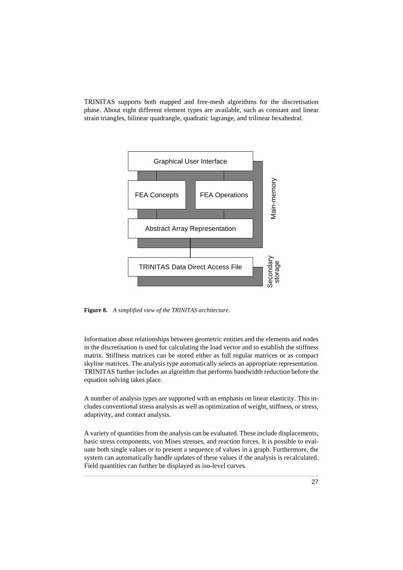
The TRINITAS program is “model-oriented” rather than file-oriented and does not in-corporate any data or result files. Instead, all model interaction is performed through thegraphical user interface that accesses main-memory data structures representing theanalysis model. TRINITAS is further designed in a highly structured, “object-based”,manner with specific sets of procedures for each concept class, such as point, line, sur-face, and volume. The design is also layered with well-defined interfaces between thelayers. A simplified view of the different layers is provided in Figure 8. These layersinclude the graphical user interface level, the application concepts layer including FEA-

1. The ODMG standard originates from the Object Management Group (OMG), Framing-ham, MA, USA.

26

related concepts and operations, the abstract array layer, and the data file layer for sec-ondary storage. Additional interfaces exist for communicating with, for example,graphical devices. All data in the application layer is stored in main-memory using theabstract array representation and storage and retrieval to and from secondary storage ishandled automatically by the system. The TRINITAS system currently consists ofabout 2200 subroutines of FORTRAN code and a small part of C code to interfacegraphics libraries.

Figure 7. Example of the graphical user interface of TRINITAS.

The geometry is the central concept when specifying an analysis model in TRINITAS.A analysis geometry is built up from basic geometric entities, such as points, lines, sur-faces, and volumes. When the geometry is specified, it can be extended with differentforms of boundary conditions, such as point loads, distributed loads, fixed or prescribeddisplacements. The domain properties are provided by default if nothing else is speci-fied. Hence, the problem to be analysed can be completely specified before one consid-ers how it should be discretised. This makes it possible to change the discretisationwithout respecifying the boundary conditions.

27

TRINITAS supports both mapped and free-mesh algorithms for the discretisationphase. About eight different element types are available, such as constant and linearstrain triangles, bilinear quadrangle, quadratic lagrange, and trilinear hexahedral.

Figure 8. A simplified view of the TRINITAS architecture.

Information about relationships between geometric entities and the elements and nodesin the discretisation is used for calculating the load vector and to establish the stiffnessmatrix. Stiffness matrices can be stored either as full regular matrices or as compactskyline matrices. The analysis type automatically selects an appropriate representation.TRINITAS further includes an algorithm that performs bandwidth reduction before theequation solving takes place.

A number of analysis types are supported with an emphasis on linear elasticity. This in-cludes conventional stress analysis as well as optimization of weight, stiffness, or stress,adaptivity, and contact analysis.

A variety of quantities from the analysis can be evaluated. These include displacements,basic stress components, von Mises stresses, and reaction forces. It is possible to eval-uate both single values or to present a sequence of values in a graph. Furthermore, thesystem can automatically handle updates of these values if the analysis is recalculated.Field quantities can further be displayed as iso-level curves.

Graphical User Interface

FEA Concepts FEA Operations

Abstract Array Representation

TRINITAS Data Direct Access FileM

ain-

mem

ory

Sec

onda

ryst

orag

e

28

In Appendix A, a list of main concepts and analysis capabilities of TRINITAS is includ-ed. For further information on TRINITAS functionality, the reader is referred to [11].

As a final but important note, it is worth mentioning that the “object-based” and layereddesign of TRINITAS, illustrated in Figure 8, has facilitated the integration with theDBMS in this work. The TRINITAS architecture has made it possible to transfer sub-sets of the application model to corresponding database representations. In the FEA-MOS system, the abstract array layer and the data file layer have been replaced by a cor-responding database representation by introducing an interface to the database betweenthe application layer and the abstract array layer. In addition, specific parts of the FEA-related concepts and operations could be separated and replaced by higher-level objectrepresentations within the database.

29

3 DATABASES AND DATABASE MANAGEMENT SYSTEMS

An effective operation of information assets is becoming a strategic issue in commercialactivities. Formerly, these issues were mostly emphasized in administrative areas buthave lately also got much attention in several engineering disciplines. The objective ofthe database management approach is to provide developers, administrators, and userswith generic software tools that support definition and manipulation of data in an effi-cient, uniform, flexible, and secure manner.

A database is, according to Elmasri and Navathe [80], a collection of related data. Da-tabases also usually incorporate further implicit properties in that the database repre-sents a specific subdomain of the real world, the data is logically structured with an in-tended meaning, and the database is produced for a specific purpose. Elmasri and Nav-athe also define a database management system (DBMS) as a general-purpose softwaresystem that facilitates definition, construction, and manipulation of databases for vari-ous applications. As illustrated in Figure 9, a database and a database management sys-tem are together referred to as a database system (DBS) and might also include otherapplication software.

A DBMS works as an intermediate layer between applications or users and data to pro-vide a generic interface to the data. It should be viewed as a tool to protect data assets,improve data quality, and to facilitate changing informations needs according to

30

Loomis [81]. These generic software tools in the DBMS can help the developers, ad-ministrators, and users to define and manipulate data in a uniform manner.

A database language (DBL), provided by a DBMS, is the actual interface for users andapplications using a database. The DBL can be an integrated language that includesconstructs for database definition and manipulation. Probably the most well-known in-tegrated database language is SQL (Structured Query Language) [82], a standardizedlanguage for relational databases. The database community usually uses the term querylanguage as a synonym for an integrated database language even though “query” refersonly to retrieving data from that database. This habit is inherited by the present author.

Figure 9. Outline of a simplified database system.

Before a database can be accessed, its content must be defined and it must further bepopulated with data. A database is defined by means of the DDL that includes con-structs for defining a database schema, i.e. the structure of the database including datatypes, relationships, and constraints, and should reflect the structure of the applicationdomain under consideration. A database schema is also referred to as the system cata-logue, data dictionary, or meta data. This schema definition is made in terms of the data

Database Databaseschema

DBMS

DATABASE SYSTEM

Users’interactive queries

Applicationsprocedures/statements

Data managing tools

Database language tools

31

model that is supported by the DBMS. A data model is a set of predefined concepts in-cluding data types and basic operators provided by the DBMS. In addition, the behav-iour of the application domain under consideration can be an integral part of the data-base definition to various levels of extent. Behaviour is specified by user-defined oper-ations on the database that are appropriate or relevant to the application domain. Thisexplicit representation and storage of the definition of the database in a database schemais a distinguishing characteristic of a DBMS compared to conventional software wheredata definition is an integral part of the application program. A DDL compiler processesthe schema descriptions into internal representations in the system catalogue.

The database can either be accessed by users directly, or indirectly, by other applica-tions. In a direct user access of the database, the user usually states either ad hoc, or pre-defined queries (also termed “canned queries”) to the database usually through a high-level query language such as SQL. Compared to a conventional and procedural-orientedprogramming language, a query language normally has a declarative nature. This meansthat you do not express the sequence or procedure for how to process your data, insteadyou declare what kind of data you are looking for. This is usually referred to as express-ing “what” instead of “how”. Ad hoc queries are transformed and optimized into an ef-ficient and executable form by the query processor before they are executed, while pre-defined queries are compiled at definition time.

Indirect access of a database, through an application, can be made by including embed-ded DML statements or precompiled DML procedures. The DML includes constructsfor retrieving, inserting, deleting, and modifying data in the database. Embedded DMLstatements are usually precompiled by a query processor before executing them where-as precompiled DML procedures are DML statements precompiled into a procedure,stored in the database, that can be called in the application.

Compilation and optimization of DDL and DML statements are made by the queryprocessing tools that also interact with the system catalogue. An executable statementis thereafter delivered to the database manager that accesses the database to store or re-trieve data. If the database is stored on disk this involves an interaction with the filemanager to access the physical data. The database manager is also responsible for sev-eral other tasks in the DBMS, including the control of authorisation, concurrency, in-tegrity constraint checking, and backup/recovery. authorisation controls the user acces-sibility of a database and can, for instance, restrict access privilege for a user to a spe-cific part of the database. Concurrency control is responsible for controlling databaseinteractions among concurrent users while preserving data consistency. Controllingdata integrity involves keeping data consistent by checking that the specified consisten-cy constraints are not violated. Backup and recovery are responsible for keeping datasafe against failure usually by making periodical and persistent backups of the databaseand keeping a log of database operations. The ability to keep the database consistent isfacilitated by defining database processing in terms of transactions. Transactions areoperations on the database that represent atomic and controlled logical processing units.

32

3.1 CHARACTERISTICS AND OBJECTIVES OF DATABASE SYSTEMS

The main objectives of a DBMS include an efficient, flexible, reliable, and secure man-agement of data. Certainly, the value and importance of these aspects vary among ap-plication areas as well as for specific purposes within application areas. For instance, insome administrative applications the efficiency of a DBS might be valued against man-ual data handling, while in computing-intensive engineering applications it must becompared to that of conventional file-processing applications. However, to meet theseobjectives a DBMS can include software tools that provide:

• Data modelling capabilities in terms of a basic data model. A data model includes aset of predefined constructs for structuring data that can involve predefined datatypes, basic operations, and user-defined data structures. The structure of data is fur-ther defined into a database schema including domain concepts, relationships, andeven operations. A powerful and important aspect of data modelling is the ability ofthe user to define complex data objects and relationships. A system-supported datamodel also promotes and fosters the design and use of standardised and uniformdata representations that will facilitate reuse, communication and exchange of dataamong applications and within organisations.

• A high-level database language, usually referred to as the query language, that pro-vides the interface to the database. The DBL can be used directly and interactivelyfor defining, manipulating and querying of data. DBL statements can also be em-bedded in a host language (the implementation language of the application) for in-directly accessing data in the database. In a DBL, data management is usually spec-ified more declaratively than in a conventional programming language.

• Persistent storage of data, i.e. data (and program procedures) can be stored perma-nently on secondary storage and thus will survive termination of program executionand can later be retrieved. Transferring data between a DBMS and applications cangive rise to what is called an impedance mismatch problem which has to be ad-dressed. The impedance mismatch problem implies that the application and theDBMS have incompatible data representations, meaning that when data is ex-changed it must be transformed. An approach to solve this problem is to be able tostore and manipulate programming language objects (e.g. C++ or Smalltalk objects)persistently in the database which is the approach applied in some OO DBMS.

• Efficient accessibility of data. DBMSs support facilities for creating access struc-tures, or indexes, that make access of data elements efficient. There are general in-dexing techniques, such as various tree data structures and hash tables, and tech-niques specialised for certain types of data, such as quad trees for spatial data. TheDBMS also usually has facilities for optimizing queries, i.e. transforming a queryinto a form that has an effective execution order.

• Logical and physical data independence by views and language mappings. Data in-dependence means that there is a separation between two software layers in such away that there is no need for the “upper layer” to know anything about the data or-ganisation or the data access techniques in the lower level. Data independence be-

33

tween the internal schema and the conceptual schema in a DBMS is referred tophysical data independence since the conceptual schema needs no knowledge ofphysical data storage. Likewise, when the external schema does not need completeknowledge of the conceptual schema, it is referred to as logical data independence.It should be possible, for instance, to add information about an entity or add newentities to the conceptual schema without affecting the external schema. The DBMSaccomplishes data independence by language mappings between different schemasand restricting certain operations to a specific schema. More complete discussionson issues in data independence are given in Date [83].

• Data sharing through concurrency control and transaction processing. Operations ina DBMS can be performed as transactions that are logical operation units on the da-tabase. The transaction processing software controls the state of transactions andguarantees that the database is always in, or can return to, a consistent state. Further,the DBMS can use concurrency control to ensure that several users can access andupdate the same data element in a controlled manner and guaranteeing a correct re-sult. Thus, transactions and concurrency control ensure multiuser transactions to beperformed correctly and several users can share data without bothering about inter-fering with other users.

• Access control through authorisation tools. Not every user might be allowed to ac-cess the complete database and to control this, the DBMS must include security andauthorisation software. authorisation can, for instance, be specified in terms of priv-ileged commands or software, or by allowing database access through a set ofviews.

• Different levels of fail security through facilities for logging, backup, and recovery.To assure that the database can be recovered from different types of software andhardware failures the DBMS include facilities for logging of transactions, makingbackups of the database, and recovery procedures to recover from failures and re-store the database into its last consistent state.

• Another type of data security can be controlled to some extent by redundancy con-trol, certain inconsistency control, and integrity constraints. Redundancy can be re-duced by sharing data among applications. Limited redundancy can also be control-led by automatically propagating updates in the database to avoid inconsistencies.Even without redundancy there can be data inconsistencies. A data element can beupdated with an inaccurate value in reference to itself or to some other data element.This type of inconsistency is controlled by adding integrity constraints in the data-base that can be controlled by the DBMS.

• Active behaviour can be introduced into the database through the addition of declar-ative rules and inference procedures (or deduction). By representing rules thatshould perform some defined action when some conditions are fulfilled an activebehaviour can be achieved in the database.

• There is a well-known architecture for describing databases called the three-schemaarchitecture [84]. Its aim is to isolate the physical database from applications. Fromthe lowest level, the first schema is the internal schema that describes the physical

34

storage structure of the database in terms of the physical data model and accessmethods. The second level, the middle level, involves the conceptual schema and isa general conceptual representation of the problem domain. It describes entities,structures, and operators in terms of a data model without physical considerations.The third level represents the external schemas (or views) and describes subsets ofthe conceptual schema that are relevant to, and in a form suitable for, particular ap-plications.

3.2 CONVENTIONAL DATABASE TECHNOLOGY

Various criteria can be applied for dividing DBMSs into certain categories. Usually, theunderlying data model works as a base for such a division but you can also see divisionaccording to, for instance, usage profile, distribution, or structure of the DBMS. If westart with the data model, there are basically the hierarchical, the network, the relational,and the object-oriented data model.

Figure 10. The evolution of DBMS technology.

3.2.1 Hierarchical database management systems

In hierarchical DBMSs data is arranged in hierarchical tree structures of connectedrecord types. Data manipulation in the hierarchical model is accomplished by embed-ding data manipulation operators in a host language. There are a set of operators fornavigating in the tree structure and operators for “updating” data in a record-at-a-time

fashion. One of the earliest and most widespread hierarchical DBMS is IMS1 (Informa-tion Management System).

1. IMS is a product of the IBM Corporation.

1960 1970 1980 1990 20001950

FilesHDBMS

NDBMS

RDBMS

SQL (ANSI)

OODBMS

ORDBMS

SQL2

... OQL, SQL3

35

3.2.2 Network database management systems

Data represented in the network model is arranged in network structures represented byrecord types where interrelationships are represented by set types. A set type representsa one-to-many relationship between two record types. As for the hierarchical model,data manipulation is done by means of operators for navigating in the network and byrecord-at-a-time operators for updating data stored in the records. The data manipula-tion commands are also in this case intended to be embedded in a host language. The

network model is often referred to as the CODASYL1 (Conference on Data SystemsLanguages) model and an example of a commercial CODASYL-based DBMS is

IDMS2.

3.2.3 Relational database management systems

The relational data model is based on a single uniform data structure called a relationthat is used to represent both data and interrelations. A relation is commonly viewed asa named table where rows are called tuples and where columns contain attributes. A ta-ble can represent both a class or a relationship between classes. When the table repre-sents a class, the tuples represent specific instances, of that class and the attributes rep-resent common properties for the class. Similarly, a table can be used to represent a re-lationship, whose instances are represented by rows in the table. In this case, thecolumns represent the participating entity types. Further, relationships can be of n-arytype where n states the number of columns in the relation.

Different types of constraints can usually be defined on relations in order to control theconsistency of data. The different types of constraints include domain constraints, keyconstraints, and entity integrity and referential integrity constraints. These are used tocontrol that the value domain of attributes is correct, that tuples are uniquely defined,and to maintain consistency among tuples.

Data manipulation on the relational model is usually made through a high-level querylanguage, usually SQL, that includes both procedural and nonprocedural constructs.The term query language associates only to retrieval operations, but in addition, a gen-eral query language usually includes operations for data definition, and update. For up-dates of relations, there are three basic operations for inserting, deleting, and modifyingtuples. Section 3.8 presents more about data management in R DBMSs and SQL.

Compared to older data models, such as the hierarchical and the network models, therelational model is more independent from its physical implementation. It also has amore formal basis since its simple and uniform base model has made it possible to de-

1. Originally defined by the CODASYL Data Base Task Group in 1971.2. IDMS was originally a product of Cullinet Software, Inc., and is currently marketed un-

der the name CA-IDMS by Computer Associates.

36

rive a relational algebra and a relational calculus that is based on mathematical theories.An important reason to the success of R DBMSs, is the availability of declarative queryfacilities in SQL.

Examples of well-known commercial R DBMSs are ORACLE1, Sybase2, INGRES3,

INFORMIX4, and DB25.

3.3 OBJECT DATABASE TECHNOLOGY

Classical DBMS technology concentrated on supporting administrative applications.However, in contrast to these traditional administrative database applications, scientificand engineering applications usually involve models and analysis methods of highercomplexity, Cattell [85]. This has put new requirements on existing database technolo-gy including support for domain-specific data modelling capabilities while preservingefficient data processing. It is expected that the next generation of object database tech-nology, where OO and relational database technologies are merged, can meet several ofthese needs. This also includes the availability of extensibility and main-memory resi-dency in DBMSs that are here presented as separate subsections.

3.3.1 Object-oriented concepts

Basic OO concepts that usually are supported in OO DBMS include objects, objectidentity, composite objects, methods, encapsulation, type hierarchies and inheritance,operator overloading, late binding, and version and configuration management.

• Objects form a fundamental concept of OO methodology. An object represents aphysical or abstract entity that possesses certain characteristics. Similar objects thatshare the same characteristics can usually be defined and referenced as a groupwhich is a means to introduce structure and reduce complexity in a concept domain.Other fundamental concepts of OO methodology including encapsulation, classes(or types), and inheritance are described below. In contrast to objects implementedby means of OO programming languages, OO databases provide facilities for han-dling persistent objects, i.e. objects that persist after finishing the execution of a pro-gram. Database objects can also be shared by several different applications.

• Object identity (OID) is a unique system-generated identifier for an object. By let-ting the system handle object naming and look-up, these facilities can be made moreefficient and relieve the application programmer from implementing this mecha-

1. ORACLE is a product of Oracle, Inc.2. Sybase is a product of Sybase, Inc.3. INGRES is a product of Ingres, Inc.4. INFORMIX is a product of Informix, Inc.5. DB2 is a product of the IBM Corporation.

37

nism. OID:s are used to refer to specific objects in the database (e.g. for making as-sociations between objects) or in the application program.

• Composite objects are objects that are built up of other objects, possibly in severallayers. For instance, a mechanical design can include many design details. Groupingof objects is a kind of aggregation that can be represented with ordinary relation-ships in the database. However, some DBMSs provide special treatment of aggre-gation relationships including such facilities as deleting, copying, and clustering ofcomposite objects. Composite objects are also referred to as structured complex ob-jects in contrast to the term unstructured complex objects that are used for referringto large binary objects (BLOBs) such as images, sounds, or unstructured texts.

• Attributes represent named properties of objects and can have various representa-tions. Simple attributes are used to describe properties that can be represented by lit-eral values such as integers, reals, or strings. Complex attributes consist of referenc-es, collections, and derived attributes. Reference attributes represent relationshipsbetween objects through OID:s. Collection attributes represent groups of simple at-tributes or references in the form of arrays, lists, sets, and multi-sets. Derived at-tributes are represented in terms of other attributes and the retrieval of attribute val-ues involves a computation. Some systems, like AMOS, have capabilities to auto-matically represent invertible attributes, i.e. attributes can be used in bothdirections. Normally, this capability must be represented by two relations in eachdirection that must be kept consistent. Attributes are used for representing differenttypes of relationships in OO DBMSs. Object attributes offer the most direct tech-nique for representing properties in pure OO methodology. In fact, when consider-ing real world properties in more detail, one realises that properties are actually re-lations between objects. For instance, the hardness of wooden table is related to theexposed object such as a hand or an axe. For the hand the table is hard, but to theaxe it might be soft. Another example is colour that at first thought is closely relatedto a thing but that is really dependent on the watcher’s ability to see colours. In prac-tice, we usually relate these properties to one specific type of object but sometimesa more general modelling is more convenient. By introducing functions overloadedon all arguments, Flodin et al. [19], this type of more general modelling techniquecan be used to describe relations dependent on several object types.

• Storing database methods associated with database objects in the database is an im-portant ability of OO DBMSs. However, first generation OO DBMSs do not nor-mally support the ability to store methods in the database; instead they are storedoutside the database. In many situations, domain data is more conveniently repre-sented by procedural information. This can, for instance, be a weight function thatis derived from the current geometry of a design or function that calculates the cur-rent position or velocity of a design component. By allowing procedures in the da-tabase they can be used in filtering out and reducing the amount of data that shouldbe passed to the application. Procedural information has normally been encoded inthe application programs but the evolution of OO database techniques has facilitatedstorage of procedures in the database. In pure OO systems all communication withobjects is performed through methods that hide the internal structure of the objects.

38

This is called encapsulation and provides one form of data independence.

• The structure and behaviour of objects (called the intent) are defined by types (orclasses) that are also used for controlling the type extent, i.e. the set of objects thatadhere to a certain type. Objects are used for representing types in a meta-level man-ner and define the type intent or object properties as attributes and methods. OOmethodologies usually involve some generalisation mechanism for types, providingcapabilities to structure types into hierarchies or acyclic graphs. These structures de-fine sub- and supertype relationships among types and can be used for applying var-ious hierarchical relationships. For instance, it can be used for inheritance where asubtype inherits properties from its supertypes. When a type inherits from severalparallel supertypes it is called multiple inheritance.

• Operator overloading, sometimes called ad hoc polymorphism, is one kind of pol-ymorphism that plays an important role in OO modelling. Polymorphism implies anability to have several forms. In the case of computer science, this term is used todenote various forms of sharing the same name or reference for different program-ming objects like variables and functions. Operator overloading is one form of pol-ymorphism that permits operators to have different implementations for differenttypes, or more generally for the signature for the operator. This can be accomplishedby different combinations of static or dynamic type checking, and early binding (al-so called static binding) or late binding (also called dynamic binding) of operators.The term overriding is sometimes used to refer to the situation where a type has aninherited operator name and redefines its implementation. This is a distinction fromthe more general overloading term where inheritance is not required. Examples ofadvanced use of overloaded functions for modelling linear algebraic matrix opera-tions are described in [19]. Efficient treatment of overloaded functions in AMOS ispresented in Flodin and Risch [86] and Flodin [87].

• System-supported versions and configurations facilitate the representation andmanagement of multiple variants of the same object in the database. A version is avariant of a single specific object whereas a configuration is a consistent variant ofa complex object. A configuration of a complex object includes other objects that inturn have their own (possibly different) versions or configurations. Versions andconfigurations can be used to keep different copies of, for instance, designs, to con-trol authorisation to different versions of objects, and they can also be used as toolsfor concurrency control, i.e. to coordinate work between multiple users. Several OODBMSs have basic features that support version and configuration management.

3.3.2 Object-oriented and object-relational database technology

Object database technology has evolved from two different areas. Both these strategiesto provide object-oriented functionality in DBMSs share some characteristics but alsohave major differences. What is referred to as the first generation OO DBMSs, Atkin-son et al. [88], evolved in the area of OO programming languages where the need fordatabase facilities in OO applications arose, such as the ability of storing programming

39

objects (e.g. C++ or Smalltalk objects) persistently on secondary storage. When thiskind of application terminates, objects persist on secondary storage and can later be re-trieved by another application. First generation OO DBMSs also usually include basicdatabase facilities such as a simple query language, access techniques such as hashingand clustering, transaction management, and concurrency control and recovery. How-ever, they are incompatible with R DBMSs and do not include several R DBMS fea-tures such as a complete declarative query language, meta data management, views, andauthorisation. Their advantage is a seamless integration with their corresponding OOprogramming language. Products originating from the first generation OO DBMS ap-

proach are Gemstone1, O22, Objectivity3, ObjectStore4, ONTOS5, and Versant6.

Systems called the second generation OO DBMSs evolved from the classical relationaldatabase community and were also inspired by OO ideas. The attempt to meet the needsrequired by new types of database applications, as for instance from the scientific andengineering area, has resulted in an extension of relational database technology withOO capabilities. Examples of these capabilities include object identity, object structure,composite objects, type constructors, encapsulation, inheritance, and OO extensions ofa query language. By combining this type of system with a call-level interface, it is pos-sible to provide OO DBMS capabilities to programming language-based applications.These DBMSs were first referred to as extended-relational DBMSs, Stonebraker et al.[89], but recently the term object-relational database management systems (ORDBMSs), DBMS [4], Frank [5], and Stonebraker and Moore [6], has gained considerable

acceptance. Examples of this type of product are Odapter7, Illustra8, and UniSQL9. Theresearch prototype AMOS, that is used in this work, is based on this approach. An im-portant aspect of OR database technology is the availability of several kinds of extensi-bility including query language, query processing, and storage management extensibil-ity. These issues are discussed in the next section that covers extensible database tech-nology.

These two approaches to accomplishing object database technology are currently blend-ed, Kim [90], in that the first generation OO DBMSs are extended with, for example,query languages, query optimization, views, constraints, meta data management, au-thorisation, triggers, transaction management, two-phase commit, and parameterisedperformance tuning. Likewise, the second generation OO DBMSs are extended to in-corporate OO concepts to be able to handle objects and OO modelling. A detailed anal-ysis of the requirements on query processing in object-relational database technology is

1. Gemstone is a product of GemStone Systems, Inc.2. O2 is a product of O2 Technology.3. Objectivity is a product of Objectivity, Inc.4. ObjectStore is a product of Object International, Inc.5. ONTOS is a product of ONTOS, Inc.6. Versant is a product of Versant Technology, Inc.7. Odapter is a product of Hewlett-Packard, Inc.8. Illustra is a product of Illustra, Inc.9. UniSQL is a product of UniSQL, Inc.

40

provided in [6].

3.4 EXTENSIBLE DATABASE TECHNOLOGY

Extensible database technology has been identified, by Carey [91] and Carey and Haas[92] among others, as a key technology for providing database technology to newemerging database applications, such as advanced engineering applications. Applica-tions of this type usually require more powerful modelling techniques and performancethan provided by standard DBMSs. This calls for database techniques that can be tai-lored to support new data types, functions, complex objects, storage and access tech-niques. According to Carey and Haas, another motivation for this approach is to facili-tate the incorporation of emerging database technologies into existing DBMSs. Thismotivation can actually be generalised into a motivation to provide emerging databasetechnology (or software technology in general) to existing applications. Most engineer-ing applications are implemented in a conventional programming language whichmeans that large parts of the application must be redesigned and reimplemented in orderto take advantage of new software technologies. It would be much easier to take advan-tage of new software technologies if, instead, a software tool was used to develop theapplication. An extensible DBMS can, for instance, provide mechanisms for concurren-cy control and for distribution and replication of data, that would immediately be avail-able to the application developer.

Carey and Haas [92], have identified three levels of extensibility that are applicable inextensible DBMSs:

1. Data storage and access methods extensions. It must be possible in extensible data-base technology to introduce new storage structures and indexing techniques fordata. Applications are very different in their needs for specialised data structuresand access methods. For instance, numerical data is used very differently among(or within) applications. Some concepts are represented and handled as singlenumerical values that maybe should be retrieved, compared with similar data, orupdated with new values. This could be a hole diameter or a single temperature. Incontrast, other (and even the same) concepts are more efficiently represented aslarge collections of numerical data, usually in the form of arrays or matrices. Per-haps the collection should be a discrete representation of a concept that is tempo-rally or spatially distributed, such as a temperature field or a stiffness distribution.These concepts are usually involved in more complex mathematical operations thatcan be efficiently implemented using array and matrix data representations.

2. Query language extensions that include the ability of defining abstract data types(ADTs), i.e. the definition of new data types and their corresponding operations. InOO technology this is accomplished by allowing the user to define new types (orclasses) of objects and defining operations on these types. This could even include

41

the ability to define type constructors, i.e. an ability to have parameterised type def-initions, discussed in Werner [93]. Extensibility at the query language level alsoincludes more general possibilities to extend the query language, such as definingoperations for data collections. This covers different kinds of aggregation operatorssuch as summation of numbers, counting members, or calculating averages.

3. Query processing extensions. The query processor can also be extended with newexecution strategies and new methods for combining existing operators. One mightwish to include better algorithms for join operators or new strategies for operatorordering. Furthermore, the query processor must be able to handle the new applica-tion-specific operations that the query language has been extended with. Hence, itmust be possible to add cost measures and optimization rules for these new opera-tions that should be treated by the query optimizer.

Extensibility is handled to various degrees by different DBMSs categories. In pure OODBMSs, the extensibility is accomplished only through user-defined types and meth-ods. This type of extensibility can also be available in DBMSs based on extensions ofrelational database technology but these can also provide extensible storage managersand query processors. There exist several research systems in the extensible DBMSfield built upon different basic data models. In Starburst, McPherson and Pirahesh [94],and in Postgres, Stonebraker et al. [95] (commercialised as Illustra, Stonebraker andMoore [6]), the data models are built on extensions to the relational data model. Further,the PROBE system, Goldhirsh and Orenstein [96], and the ORION system, Woelk andKim [97], are built on an OO data model. In AMOS, Fahl et al. [8], the OO data modelhas been combined with relational query capabilities. GENESIS, Batory [98], and EX-ODUS, Carey and DeWitt [99], have a somewhat different approach in providing tool-kits for generating application-specific DBMSs.

The extension of a DBMS with new data structures, operators and suchlike must alsohandle the interaction with other database facilities, such as security, concurrency con-trol, and recovery. Another problem is the interface that should bridge the gap betweenthe extensible DBMSs and the application that might be implemented in a languagewith a more primitive type system. Some efforts have been made in this area within the

ODMG standardisation where the OQL1 language, Cattell [17], is defined to permit dif-ferent language bindings for representing the data types of OQL. Using the extensibleDBMS as a powerful tool for actually implementing applications adds another view tothe interface problem. In this case, the application functionality is partly, or to a largeextent, implemented within the DBMS where more general resources can be “pluggedinto” the DBMS as modules. This raises the questions of which data structures shouldbe provided by the DBMS and where the processing should take place. By delegatingcertain application-specific operations to the DBMS one could take advantage of effi-cient data access techniques of the DBMS. This approach could further reduce the over-

1. In OQL, user-defined methods can be included in queries but they can not be handled bythe optimizer.

42

head for transporting and transforming data between the DBMS and the application.

3.5 MAIN-MEMORY DATABASE TECHNOLOGY

Main-memory (MM) DBMSs have evolved during the last few years, DeWitt et al.[100] and Eich [101]. Conventionally, databases are disk-based, i.e. they reside on asecondary storage media, usually in the form of magnetic harddisks. However, hard-ware developments such as large main-memories and fast networks have provided po-tential for new design ideas. This has cleared a path for the development of MMDBMSs that assume that the entire database resides in primary memory.

There are well-known differences in the characteristics of secondary and primary mem-ory, Garcia-Molina and Salem [102], that include:

• Main-memory has orders of magnitudes lower access times than magnetic diskmemory.

• Main-memory is usually volatile while magnetic disks are not. However, non-vola-tile main-memories are becoming more common.

• Magnetic disks have a high initiation cost for each access that is independent of theamount of data that should be retrieved. This fact makes this kind of storage devicesblock-oriented. Main-memory has low initiation cost and consequently needs noblock-orientation.

• Sequential access is faster than random access for magnetic disks. This does nothold for main-memories since they are really random access memories. Thus, dataorganisation and clustering are more important for disk storage.

• Main-memory data can be more vulnerable to software errors than disk-residentdata since main-memories can be directly accessed by processors.

Disk-based database systems cache data from secondary to primary memory forprocessing. In contrast, an MM DBMS can have a copy of data on disk for backup pur-poses. Hence, both architectures have data located both in main-memory and on diskbut MM DBMSs have their principal copy in memory while disk-based DBMSs havetheir principal copy on disk. These differences considerably influence the design forthese two database system architectures. Since disk access is the bottleneck for disk-based systems, they are designed with data structures, access methods, and clusteringtechniques that should minimise disk access for reading and writing data to disk. Main-memory database systems access data directly in memory which results in better per-formance than conventional disk-based database systems. For main-memory systems itis instead the processing time that is the origin for the performance. Garcia-Molina andSalem [102] mention performance considerations as especially important to real-timeapplications. However, performance can also be of vital importance in other engineer-ing tasks such as interactive engineering applications for design and analysis that in-

43

volve computing-intensive calculations and simulations. Performance is not only ac-complished through main-memory residency; at least as important is query optimiza-tion that can reduce the combinatorial complexity of queries by several orders ofmagnitudes. Litwin and Risch [103] show that a combination of main-memory residen-cy and query optimization is required for best performance. This technique can actuallyreduce execution time to less than one disk access in some situations which would beimpossible with traditional disk-based techniques.

Access methods and data representations are additional issues that are effected byswitching from disk-based to main-memory-based technology. Specialised accessmethods are utilised to take advantage of main-memory characteristics. For instance,there are methods based on hashing techniques, special tree representations, or pointer-based indexing. Data representation techniques must also be adapted for main-memory.Furthermore, the query execution cost is determined by the processing cost instead ofthe cost for disk access as in disk-based systems, as discussed in more detail in Listgar-ten and Neimat [104]. Concurrency control, transaction and recovery processing, anddata clustering and migration are also mechanisms that need specialised treatment, Gar-cia-Molina and Salem [102]. The techniques for exchanging data between applicationsand the database also need adaption to main-memory residency of the application pro-gramming interface.

MM DBMSs, are exemplified by SmallBase, Listgarten and Neimat [104] and Heytenset al. [105], WS-IRIS [103] and AMOS [8]. SmallBase is built upon a relational datamodel, whereas WS-IRIS and AMOS are based on an object-relational data model. Amain design idea behind main-memory, as well as extensible, database technology isthe ability to use these types of DBMSs embedded within applications.

3.6 ADDITIONAL DATABASE TECHNOLOGIES

3.6.1 Distributed database management systems

DBMSs can be centralised or distributed. A centralised DBMS resides on a single com-puter site that includes the complete database and the DBMS software and hardware.Distributed database management systems [106], D DBMSs, take a contrasting ap-proach, i.e. the data and software are distributed over a hardware platform that consistsof multiple computer sites that are connected by some form of communication network.There are different potential benefits that motivate the use of D DBMSs that include:

• Distributed databases can naturally conform to distributed applications. Databaseapplications may be physically distributed (different locations) or logically distrib-uted (different application domains) that require or make it convenient to distributedata over several sites.

• The reliability and availability can be increased since redundancy can be introduced

44

by replicating data and functionality over several sites.

• Controlled data sharing can be provided by keeping local control over data but al-lowing distributed access.

• Performance can be increased due to the distribution of transactions over multiplesites that would otherwise be processed at a centralised site.

Distributed database systems can further be divided into various categories dependingon additional factors such as the level of homogeneity, autonomy, and transparency.

Distributed database systems can have different levels of homogeneity. In a homoge-nous database system the same DBMS is used on both servers and clients, which is notthe case for heterogeneous database systems.

There can further be different levels of autonomy in D DBMSs. At one end of the spec-trum we have no autonomy where a D DBMS acts as a centralised DBMS with a singleconceptual schema and the access must be made through one server. At the other endwe have federated DBMSs or multidatabase systems where each server has an inde-pendent DBMS. It is then possible to have local databases and transactions that providea higher degree of autonomy. Global clients can then, through a multidatabase interface,access privileged parts of the collection of autonomous databases (that form the multi-database).

Another aspect of distribution of databases is the degree of distribution transparency ofthe system. Does the user need to now anything of where data is distributed and of howdata is fragmented or replicated? In a transparent system this knowledge is not neededbut is required to some extent in systems with a lower transparency level.

Technology for D DBMSs can be of great importance in applications for engineeringdesign and analysis where different engineering domains withhold their own databases.Certain parts of that data must be shared among several disciplines and further be keptin consistence at the global level. The role of D DBMSs in engineering applications isbriefly discussed in sections Section 3.7, Section 6.2, and Section 5.1.

3.6.2 Active database management systems

Database systems have traditionally been passive, i.e. the communication between theusers or applications and the DBMS have been triggered by the former. In contrast, anactive database management system can in itself react and act on database events (e.g.database updates) or external events (e.g. updates of physical signals). Active function-ality is commonly accomplished by providing some form of rule system in the DBMS.Rules usually consist of a condition part and an action part. The condition part definesthe event situation that should be true for executing the operations defined by the actionpart. Actions can consists of database operations and external operations. When the rulesystem detects relevant events it triggers the condition monitoring and, if the condition

45

part evaluates to true, the action part is executed.

The active database functionality can be used to provide consistency control as an inte-gral part of data management. For instance, constraint management can use rules thatdetect and abort transactions that attempt to perform updates that violate database con-straints, Ceri and Widom [107], Kim [90], Risch and Sköld [108], Sköld [109], Sköldand Risch [110].

Explicit declaration of rules for data consistency and consistency handling within theDBMS can increase the flexibility of consistency control and the reliability of data. Byintegrating the rule system within the DBMS, the data exchange between an applicationand a database can be reduced and, furthermore, query optimization techniques can beused for accomplishing efficient rule execution.

The ideas of active DBMS technology are influenced by the fields of knowledge-basedand expert systems, expert database systems, and deductive DBMSs. Techniques fromthese fields, like rule-based reasoning and inference techniques, have been adapted tosuit needs emphasised in the database area, such as handling large data sets and efficien-cy-related considerations.

Active behaviour in AMOS is treated in Risch and Sköld [108], Sköld [109] and Sköldand Risch [110], that describe the extensions of AMOS with efficient change monitor-ing techniques using active rules. These techniques could, for example, be used for con-straint checking in model preparation and result evaluation and for controlling solutionparameters in the engineering analysis process.

3.7 SCIENTIFIC AND ENGINEERING DATABASE TECHNOLOGY

The database field can also be divided into different application areas where the require-ments on the database technology can vary heavily. The field of scientific and engineer-ing database technology is the most relevant for this work.

Classical DBMS technology was primarily designed for conventional applications ofbusiness and administration that were characterized by large amounts of data with rel-atively simple structure, and where the operations on data were small and simple aswell. However, as for instance pointed out by Cattell [85], these techniques have hadless to offer to more complex software applications for supporting mechanical engi-neering, electrical engineering, document handling, software and systems engineering,process control, science and medicine, expert systems, and advanced financial applica-tions.

The field of scientific and engineering applications has been especially emphasised byseveral authors, Cattell [85], Navathe and Elmasri [80], Korth and Silberschatz [111],Loomis [81], and Ullman [112], as an important field for future database support. In the

46

literature there exist a division of database applications into scientific databases and en-gineering databases. The term “scientific” is usually associated to areas such as life,earth, space sciences and suchlike where large amounts of “real” data (experimental ormeasured data) is handled. On the other hand, “engineering” refers to typical engineer-ing issues of producing articles from mechanical or electrical components (such as nuts,bolts, and resistors) to complete complex products or systems (such as cars, aircraft,power plants, and computers). The engineering process can in itself be quite complexincluding several different subprocesses that should be coordinated. For instance a me-chanical design should be specified, designed, analysed, manufactured, tested, main-tained, and possibly re-cycled; manufacturing should be prepared and manufacturingtools should be produced, for instance. A simple product might involve just a few peo-ple within an enterprise while a more complex product requires the engagement ofmany employees with different skills that might span several enterprises. In the engi-neering field a large amount of data is “synthetic” (that is generated by design tools asCAD software, or simulation tools).

More specifically, conventional database applications were, according to Korth and Sil-berschatz [111], characterised by:

• Uniform and equal-sized data items.

• Record-oriented and fixed-length data items.

• Small data items.

• Atomic fields. Record-fields are unstructured and of fixed length.

• Short transactions with an execution time of fractions of a second.

• Conceptual schema changes are infrequent and usually involve only simple modifi-cations.

Much of the effort in research and development of new database technology aims atsupporting those kinds of new emerging database applications mentioned above. Com-pared to classical database applications, these applications usually deal with a morecomplicated problem domain. They require the representation of a much broader spec-trum of domain information that involves complex composite concepts of several typesand of non-uniform data items, complex concept structures, associated operations, anddomain knowledge. The conceptual structure also evolves during its life-cycle meaningthat the schema will be exposed to more changes. Further, the usage profile can also bequite different as data should usually be shared among several project members in acomputing environment. Specific data processing activities typically have much longerduration in these applications and data exists in several versions which must be keptconsistent. The application part will usually contain much functionality and it is of ma-jor importance to have a good programming language interface to achieve efficientcommunication between the application part and the DBMS. It is also required that thedatabase application has a performance of, at least, the same level as a conventionallyimplemented application. Specifically in engineering applications, data usually incor-

47

porates the following characteristics:

• Engineering designs are in general represented by collections of non-homogeneousdata objects. A specific design object is typically a composition of other design ob-jects that form a more complex structure than those found in conventional DBMSapplications. Further, these object compositions usually include many domain-spe-cific relationships. These relationships can be of various types, such as mechanical,mathematical, spatial, and temporal relationships, and are important in engineeringapplications for representing the structure and functionality of the design. In addi-tion, this type of relationships might need special treatment in the database concern-ing data structures and access techniques.

• Derived data, i.e. data computed from basic data elements, is important in engineer-ing applications. This type of data can require a recalculation whenever any under-lying data element is updated. For instance, the weight of a design and any otherquantity dependent on the weight must be updated whenever the geometry ischanged.

• Engineering data involves many domain-specific types where each type does notneed to include a large amount of instances. However, a complete design can in itsentirety represent a substantial amount of data.

• Engineering domains include a lot of domain knowledge that governs the permissi-bility and consistency of data. At present, this type of knowledge is usually embed-ded within applications or explicitly handled be users. By extracting domain knowl-edge, from applications and users, and representing it as meta-knowledge in the da-tabase it will be represented more explicitly and become easier to manage.

• Engineering data objects are usually built up by several basic data types for literal,numerical, and image data (BLOB’s). Numerical data is a central component of en-gineering data and is usually used in aggregate data items such as in arrays, vectorsand matrices. These numerical data types are used in describing higher-level engi-neering elements, such as geometries formed by complex compositions of basic ge-ometry elements. Conventional commercial DBMSs do not normally support datastructures suitable for engineering applications; they mainly support basic datatypes such as character strings, integers, and floats (not always). However, thesesystems will evolve and provide more complex data types as well and with the in-troduction of OO DBMSs, this fact does not hold since these usually support aggre-gate and user-defined data types. On the other hand, this will probably not beenough. Advanced engineering applications will always demand specialised datatypes, such as compact and efficient matrix representations optimized for specificapplications. Extensible DBMSs are able to provide this functionality.

• The domain-specific functionality and behaviour are important aspects of engineer-ing design that one would like to capture in the database. For example, how a certainmechanical connection is allowed to move and if it is dependent on other parts inthe design. Representing functionality and behaviour usually includes some kindsof computations that can be represented by allowing the representation of functions

48

and procedures in the database.

• Engineering data structures are in general more exposed to change compared to datastructures in conventional DBMS applications. Engineering designs evolve contin-uously during the development process in comparison to conventional database ap-plications where the structure of data is more static.

• Transactions in engineering applications are typically of longer duration than nor-mal database transactions that last for fractions of seconds. Design and analysis ac-tivities may take hours, days, weeks, and even longer to perform. CommercialDBMSs use locking-techniques that assume transaction times of a few seconds.However, specific engineering activities can include smaller transactions like up-dates of a local design that must be kept consistent. Thus, engineering applicationscan involve the complete scale from short to long transactions. The profile of up-dates of engineering design is also quite different from conventional updates thattypically should update single values. It is not uncommon that updates in engineer-ing applications are far-reaching since many geometrical, topological, and function-al relationships involve many related objects. Changing a single design object canimply updates of many related design objects.

• Engineering design and analysis systems must provide configuration and versioningsupport. A design passes through several design stages where it can exist in severalrelated versions and where each version has its own state, specifying if it is releasedor is in any other relevant state. The design support system must also permit engi-neers to work on their own private or local design that is extracted out of and can bemerged into a public or global design representation.

• Engineering computing environments can be of various complexity from single per-sonal computers to large networks of work stations and including special servers fordata storage (DBMS servers) and processing (super and parallel computers). Atleast in the complex case, data can be distributed over the complete network whereresponsibilities for specific parts are distributed on specific organisational func-tions. For instance, there might be different persons who are responsible for geom-etry data, materials data, and test data. The data that represent the current and com-plete design can therefore be distributed over the network and subsections of datado not need to be in the same state at any time. There can also, as already mentioned,be local copies of specific design objects or other associated objects such as variousanalysis models. For instance, for performing some type of mechanical analysis youmight need to retrieve geometry, material, and loading data from different sourcesinto your analysis model. The analysis can thereafter be carried out and perhaps it-erated before a satisfactory result has been accomplished. The iteration processmight require alterations of data and data exchange between the local and globallevel. At certain “check-points”, inconsistencies between these levels must be re-solved and updated. Thus, DBMSs might be involved for data management on boththe local and global level for sharing, exchanging, and combining data and for main-taining consistency between levels.

• Engineering designs can include a lot of repetitive data in forms of nuts and bolts,

49

form features like holes, fillets, or notches. For this type of design object, only dis-tinct values need to be stored for every instance and general properties can be re-used.

• Engineering applications usually have higher requirements on execution perform-ance than conventional applications. Data is typically used in highly interactive andcomputing-intensive tasks with high performance requirements that should bematched by the DBMS as well.

• The amount of engineering data in a design project can be huge. These levels areexpected to rise since more design, analysis, testing, and manufacturing activitiesare being computerised and more data is being generated in each activity. DBMSsfor engineering applications must be able to cope with these amounts of data.

Computational mechanics forms a sub-area of mechanical engineering where efficientcomputing support is obligatory. In this area, finite element analysis is utilised for ana-lysing and simulating different phenomena such as mechanical, thermal, fluid, or acous-tic. FEA software should handle large complex analysis models and algorithms in acomputing environment that involves several other software tools. In this area, databasetechnology can be introduced for a number of reasons and tasks including:

• The administration and management of FEA models and simulation results, both lo-cally or globally. This involve administrating geometry, material, and load data,complete analysis models, analysis results, and the relations between FEA data andcorresponding design objects. There are also other administrative data not directlyrelated to FEA, such as design project data, that can be relevant for this task as well.

• Sharing, exchanging, combining, and transforming data among different tools andusers. The same basic data, such as data regarding the geometrical form of the de-sign, might be used by several users or tools. If different tools use the same data butin different formats, data must be transformed to the appropriate format for specifictools. The DBMS can provide a uniform and standardised data representation thatsuits different tools. Furthermore, a DBMS can be a powerful medium for exchang-ing data between tools. Geometrical data generated in a CAD program might becombined with load data from some load handling program, and it can be providedto an FEA program by means of a data-based representation and retrieval.

• Extending the domain functionality of FEA applications. Additional functionalitycan be added to FEA systems by representing and utilising domain knowledge, suchas different types of constraints on, or rules for, the FEA domain. For example, theDBMS can check if finite elements are too distorted or if calculated stresses exceedsome critical level. Some commercial DBMSs currently provide mechanisms fordefining rules that can detect and react when a certain condition is fulfilled in thedatabase.

• Extending the system functionality of FEA applications. If an FEA application istightly integrated with or developed by means of a DBMS, the final application cantake advantage of generic DBMS techniques for data management including data

50

sharing, distribution and replication of data, concurrency control, transactionprocessing, persistency, backup, and recovery. Furthermore, the DBMS provide theapplication with a data model, storage management, and a query language and proc-essor that support application modelling.

• Development, evolution, and maintenance of FEA software. By using generic soft-ware developments tools, such as a DBMS, applications can be defined at a higherconceptual level than is normally done in conventional applications. Data is mod-elled and manipulated at a higher level resulting in more flexible, composable, andreusable models. Generic subsystems of the DBMS (see previous item) can be useddirectly and need not be re-implemented and a great deal of low level implementa-tion details can be avoided. This will restrict, isolate, and reduce complexity of thoseparts of the application that concern the actual problem domain resulting in an ap-plication that is easier to maintain, evolve, and further develop.

The items concerning FEA and listed above can to various degrees be accomplishedwith database technology of today. In general, the first three items can involve a DBMSthat is loosely coupled to the FEA program. Data can be stored in and retrieved fromthe database but most of the application functionality is kept within the FEA program.The DBMS will complement the FEA program by supporting pure DBMS facilities.The latter two items involve a more tight coupling between the FEA program and theDBMS. In this situation, database technology is used for developing, and to be an inte-gral part of, the FEA application. Domain-specific functionality is here transferred fromthe FEA program to the DBMS. Various architectural considerations for tightly coupledsystems are further discussed in Section 5.1.

Database technology for scientific and engineering databases has, in for example [1] [2][3], been identified as an area where further research is needed to develop database tech-nologies that meet the requirements of these applications. Much attention has recentlybeen paid to OO DBMSs which are considered to be specifically suitable for this typeof application. A number of characteristics that favour object-oriented models havebeen pointed out by Navathe and Elmasri [80] and Cattell [85]. Object-orientation pro-vides modelling that is isomorphic to the problem domain, provides complex modelstructures, has uniformity of data access, and provides extensible models resulting in ahigher level of modularity and flexibility of the models. The referenced and additionalmechanisms that OO DBMSs provide for supporting advanced data management in-clude:

• Unique system-provided object identifiers are convenient in engineering applica-tions that typically deal with unnamed design objects such as point, lines, and sur-faces in a geometrical model.

• Composite objects are everyday things in the engineering world.

• Referential integrity is important for maintaining consistency within complex engi-neering models.

• Object-type hierarchies provide an important mechanism for structuring engineer-

51

ing data.

• Ability to store associated procedures in the database supports representation of do-main functionality.

• Object encapsulation can hide implementation details and provide limited data in-dependence, but does also restrict the expressibility that can be inconvenient in cer-tain situations.

• Ordered sets and references are very useful in engineering applications where theorder among objects is used in many situations.

• Large data blocks are applicable, for instance for representing large numerical ma-trices.

• A programming language interface is important for integration with applicationsand for representing domain operators.

• Multiple database versions must be supplied for representing engineering designversions.

• Long-term lock and check-out mechanisms must be supplied to conform to engi-neering design tasks.

• Efficient remote and local database access is important since engineering models in-clude large amounts of data that should be processed and presented to the user.

• Single-user performance is very important since most engineering applications pre-suppose interactive computer-intensive usage.

• Ease of schema changes supports the representation of evolving designs.

However, DBMSs for new advanced applications also need the support of traditionaldatabase facilities, which is emphasized by Cattell [85] and Stonebraker et al. [89]. Therequirements that engineering applications would benefit from are here presented withcomments on the relation to the previous discussion on engineering data, and are as fol-lows:

• Ability to store and handle large volumes of structured data persistently.

• Access to query language facilities. A query language in its general meaning, in-cluding data definition and manipulation is a powerful tool to model and manipulatedomain data. Advanced applications, such as in the field of computational mechan-ics, require extensible query languages that permit the definition of domain opera-tors.

• Tools for designing application user-interfaces. Traditional forms-based interfacesmight be useful for administrating engineering data but are not for design and anal-ysis applications where much data is distributed over space and time. However, newadvanced GUI tools might support the design of form- and geometry-related inter-faces that can be useful.

52

• Capability of distributed databases can be important for storing engineering data onseveral servers in a network.

• Support for triggers or more advanced active rules can be useful for specific taskssuch as automatic checking of analysis results and other design constraints.

• Fine-grained concurrency can be required along with long-running transactions inengineering applications.

• Crash recovery capability for keeping an engineering database consistent is desira-ble.

• Data independence is an important aspect since it is a basic mechanism for sharingdata among applications and it is a means to raise the conceptual level in data mod-elling.

When the application of database technology in advanced engineering applicationsspreads, the requirements on DBMSs will be further widened. One such requirement isthe ability to do analysis and synthesis of data in the database, i.e. data should be proc-essed, analysed, and synthesised by domain-specific database operators instead oftransferring data into the application for processing. This has already received attentionin other areas such as in geographical informations systems (GIS) [113], chemistry[114], and advanced financial applications [115].

For applications that require specialised data structures, perhaps in combination withadvanced processing algorithms, extensible DBMSs can provide key technology forimplementing these applications. The DBMS can be extended with new data structuresand access techniques that can be seamlessly managed by the system. One examplewould be numerical analysis algorithms that are usually based on compact and efficientmatrix representations, such as skyline or sparse matrix representations. These special-ised representations need dedicated operators for numerical algorithms in linear andnon-linear algebra, and mathematical programming, for example. This approach will befurther discussed in Section 4.1.

A closing comment regarding scientific and engineering data management; there is re-ally no clear distinction between the areas of science and engineering. The engineeringfield also involves much “real” data, such as test data from different activities, and sci-entific work involves simulated data as well. Further, many computing tools are used inboth science and engineering. Programs for FEA are used in industrial product devel-opment as well as in research in the computational mechanics field and others.

3.8 QUERY LANGUAGES FOR DBMS

The term query language is commonly used as a synonym for database language(DBL), i.e. the language interface to the DBMS. These terms where introduced earlierin this chapter but will here be presented in more detail and complemented with somegeneral issues and directions of query languages. Query languages are usually higher-

53

level languages than ordinary programming languages. The query language is the actualdata management language that is used for defining, updating, and querying data in thedatabase. Sometimes, the term query language is only used to refer to the pure querylanguage, i.e. the part of a database language that concerns querying of data and not datadefinitions and updates. It is also quite common to view the database language interfaceas a collection of languages for different purposes that include a data definition lan-guage (DDL) for data definition and schema management, and a data manipulation lan-guage (DML) for updating and querying the database. The data definition is sometimesfurther separated into a DDL, a storage definition language (SDL) for defining thephysical storage schema, and a view definition language (VDL) for defining databaseviews.

General query languages were first developed for R DBMSs and included SQL, themost well-known query language that has become the standard query language for RDBMSs. Other examples of relational query languages are QBE and QUEL.

The field of OO DBMSs still lacks a unified and standardised data model and even morea unifying query language. However, standardisation efforts are currently being madein this area within the SQL community, through SQL3 ISO/ANSI [16], and in the OMGcommunity, through OQL ODMG [17]. A few commercial products do currently offerobject-oriented query facilities like for instance, OpenODB, UniSQL, and Illustra.Likewise, our AMOS OR DBMS research prototype also include object-oriented queryfacilities through AMOSQL. The current trend in this area is to combine relational andobject-oriented database technologies to achieve object-relational query capabilities,i.e. the powerful query capabilities of relational query languages extended for object-oriented data models, Kim [90].

3.8.1 Relational algebra and relational calculus

It is common to characterise query languages as being procedural or nonprocedural (al-so declarative). With a procedural language you specify how to compute the expectedresult, whereas by means of a nonprocedural language you specify the desired resultwithout any computation strategy. Procedural and nonprocedural query languages canbe considered as two basic language forms. Most commercial database languages in-clude both nonprocedural and procedural parts as in the case of SQL that include a non-procedural query language.

Two formal query languages, relational algebra and relational calculus, have been de-fined for the relational data model.

Relational algebra is a procedural query language that defines a collection of operationsfor manipulating entire relations. These operations take relations as input and producenew relations as output. There are operations specifically defined for relations as wellas set operations from set theory. Examples of the former include select , project , and

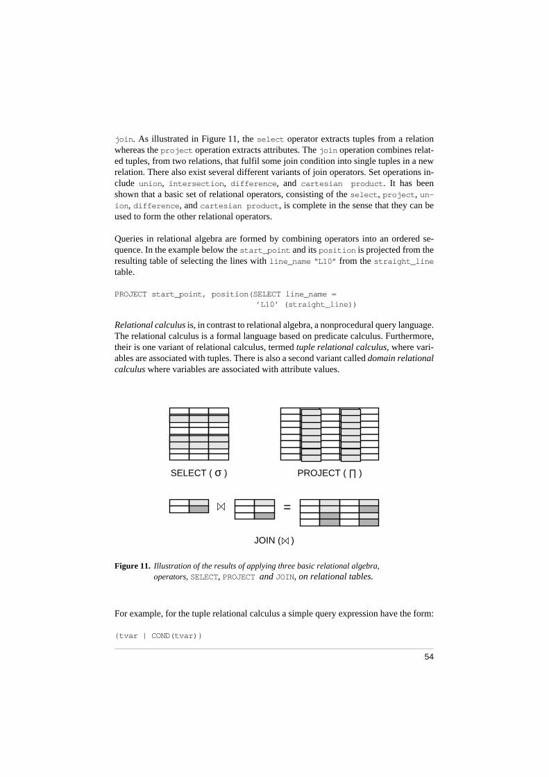
54

join . As illustrated in Figure 11, the select operator extracts tuples from a relationwhereas the project operation extracts attributes. The join operation combines relat-ed tuples, from two relations, that fulfil some join condition into single tuples in a newrelation. There also exist several different variants of join operators. Set operations in-clude union , intersection , difference , and cartesian product . It has beenshown that a basic set of relational operators, consisting of the select , project , un-

ion , difference , and cartesian product , is complete in the sense that they can beused to form the other relational operators.

Queries in relational algebra are formed by combining operators into an ordered se-quence. In the example below the start_point and its position is projected from theresulting table of selecting the lines with line_name “L10” from the straight_line

table.

PROJECT start_point, position(SELECT line_name = ’L10’ ( straight_line ))

Relational calculus is, in contrast to relational algebra, a nonprocedural query language.The relational calculus is a formal language based on predicate calculus. Furthermore,their is one variant of relational calculus, termed tuple relational calculus, where vari-ables are associated with tuples. There is also a second variant called domain relationalcalculus where variables are associated with attribute values.

Figure 11. Illustration of the results of applying three basic relational algebra, operators, SELECT, PROJECT and JOIN, on relational tables.

For example, for the tuple relational calculus a simple query expression have the form:

{tvar | COND(tvar)}

PROJECT ( ∏ )SELECT ( σ )

JOIN (__)

=

55

where

tvar

is the set of all tuples that satisfy the conditional expression

COND(tvar)

.Simplified, a conditional expression can consist of atomic expressions including tupleranges and comparison expressions. Atomic expressions can be combined by logicalconnectives to formulas that can further include quantifiers.

The previous example for relational algebra would have the following form as a queryin tuple relational calculus:

{t.start_point,t.position | straight_line(t) and t.line_name = ‘L10’}

The domain relational calculus has a similar structure and it is shown that the expres-siveness of domain and tuple relational calculi are the same. It has further been shownthat the expressiveness of relational calculus and relational algebra are equivalent. Que-ry languages that have the same expressiveness as relational calculus are called

rela-tionally complete

query languages.

Furthermore, there are other relational data retrievals that can not be expressed bymeans of the basic set of relational operators. These include aggregation, recursive clo-sure, and arithmetic operations together with specialised variants of the basic opera-tions, such as various join methods.

Most commercial query languages for the relational model include elements of both re-lational algebra and calculus as exemplified by SQL. Other examples include the querylanguage QUEL that is based on tuple relational calculus and the graphical query lan-guage QBE, based on domain relational calculus. Commercial relational query lan-guages usually have relationally complete query capabilities and they also include com-mon extended operations. Their capabilities are extended as new versions appear andtheir more advanced query facilities will vary between products and versions.

This section has only treated retrieval capabilities of query languages but commercialquery languages also include other features covering operations for data definition, up-dates, and others.

3.8.2 The SQL language

SQL has become the standard query language for R DBMSs. It was first developed byIBM and in 1986 for the American National Standards Institute (ANSI) and in early1987 for the International Standards Organisation (ISO) an SQL standard was pub-lished, Melton and Simon [82]. A revised and expanded version, known as SQL-92 (al-so SQL2), was published in 1992. There is further ongoing work on the next generationof the SQL standard, SQL3, that aims at including support for object-orientation.

The SQL language is a general query language that copes with data definition, interac-tive data manipulation, embedded data manipulation, view definition, authorisation, in-

56

tegrity, and transaction control.

The data definition part includes operations for creating, altering, and removing tables,i.e. relations in SQL. In addition to specifying the relations in the database, the DDLincludes commands for defining: schemas explicitly, value domains, indexes, securityand authorisation, integrity constraints, and physical storage structures of relations.

Updates on relations in SQL consist of the

insert

,

update

, and

delete

commands forinserting, modifying values of, and deleting tuples in a relation.

Retrieval expressions in SQL are formed by means of the

select

statement and its ba-sic structure consist of the

SELECT

,

FROM

and

WHERE

clauses with the following syntax:

select

<attribute list>

from

<table list>

where

<condition>

where

• The

select

clause corresponds to the projection operator of relational algebra andthe

<attribute list>

is the list of attributes that should be retrieved in the query.

• The

from

clause corresponds to the cartesian product operation of relational algebra,and where the

<table list>

is the tables that should be involved in the retrieval

• The

where

clause corresponds to the selection operator of relational algebra wherethe

<condition>

is a predicate that constrains the attributes in the

from

clause.

Again, the former example would be expressed in SQL as:

select

t.start_point,t.position

from

straight_line t

where

t.line_name = ‘L10’

This was only a brief presentation of a subset of all the functionality of the SQL lan-guage. A detailed description of the current SQL2 standard is provided in Melton andSimon [82]. There is further an SQL3 standard proposal, Melton [16], in progress thatsuggests major extensions to be made to the SQL language to support object-orientedmethodology.

3.8.3 Object-oriented query languages

Object-oriented query languages are based on an object data model in comparison toquery languages for R DBMS, which usually means SQL, that are based on the relation-al data model. Hence, in contrast to relational query languages that operate on tables,object-oriented query languages are designed to operate on sets of objects.

57

The motivation is to provide query language capabilities for the object data model thatare at least as powerful as the relationally completeness of relational query languages.OO modelling is considered to be richer and more suitable for several kinds of applica-tions, including scientific and engineering applications, by providing facilities such asricher data structures, and user-defined types and operations. For instance, data typesfor numerical collections are usually supported. Furthermore, the object-oriented modelreduces the impedance mismatch between the DBMS and the application that exists forthe relational data model. Hence, the combination of an object data model with queryfacilities provides both the advantages of OO modelling and of R DBMSs, such as de-clarative data access and query optimization.

There is currently no uniform and standardised specification for an object data model.However, there are two emerging standards [116], ODMG-93 [17], and SQL3 [16], thatdefine their own object data model in combination with query facilities. Certain effortsare also made to try to merge these standards. While ODMG-93, including its query lan-guage OQL, is more related to OO programming languages, such as C++ and Smalltalk,SQL3 is built on extensions to the SQL language. The final outcome of these standard-isation efforts is not settled, and no detailed presentation of their capabilities will be pre-sented here. It is worth noting that the query language of the O

2

DBMS [117] is closelyrelated to the OQL language whereas the query language of Illustra, described in [6], isbuilt on an earlier specification of SQL3.

The AMOSQL query language, described in Section 4.3, will here exemplify the capa-bilities of an OO query language. It should be noted that AMOSQL originates from theOSQL language [15] and includes some unique features not provided in the suggestedstandards. These include overloaded multi-directional functions that have been used ex-tensively in this work. Overloading of functions on multiple arguments is included inSQL3 but not in ODMG-93. Further, the extensibility of the AMOSQL query processorthat handles optimization of foreign functions is an important property when modellingapplications-specific operations. This capability is not covered in any of the standardi-sations, but is actually provided by Illustra, and emphasised as an important mecha-nism.

59

4 THE AMOS DBMS AND THE AMOSQL LANGUAGE

AMOS (Active Mediators Object System) [8] [9] is a research DBMS prototype andconforms to systems classified as


DBMSs. An AMOS prototypehas been developed [9], built on substantial developments of the WS-IRiS main-mem-ory OO DBMS engine [103]. WS-IRiS was developed at Hewlett-Packard Laborato-ries, Palo Alto, CA, and is a derivative of Iris [118]. AMOS is further a main-memoryDBMS and assumes that the entire database is contained in main-memory. The AMOSarchitecture is tailored for main-memory usage to provide competitive performancewhich is confirmed in [103]. The database can be saved to, and restored from, disk toprovide persistency to secondary storage. Optionally, a transactional logging systemsupports logging and recoverability of committed database transactions.

The “object-relational” term presupposes the existence of a relationally complete querylanguage. AMOS includes the AMOSQL query language that provides a declarativequery interface for defining, populating and manipulating the database. AMOSQL is anextensible and object-oriented query language that is more than relationally complete.AMOSQL is a derivative of OSQL [15] which is a functional language, originatingfrom DAPLEX [119]. The AMOSQL query language is further influenced by standard-isation efforts like SQL3 [16] and OQL [17].

AMOSQL and AMOS allow extensibility at the query language level, the queryprocessing level, and at the storage management level. These capabilities are important

60

for accommodating tuned representations and operations required by demanding appli-cations. Extensions to the system can be implemented in external programming lan-guages like C or LISP (or languages callable by these).

AMOS can be operated as a single-user system, or as a multi-user system using client-server network communication. In addition prototypes of graphical interfaces to AMOShave been developed that include web-server capabilities to be able to communicatewith web-browsers.

The next section presents the mediator approach that shows how AMOS servers can beused as a mediating layer between applications and data sources in, for example, an EISenvironment. The idea of domain-specific mediators is explained. This is followed bya presentation of the AMOS architecture including the different subsystems that formAMOS and their interaction. A short introduction to the AMOSQL language is then in-cluded and, finally, this chapter is completed with a more detailed presentation of thepossibilities of extending and interfacing AMOS.

4.1 THE MEDIATOR APPROACH

Future computer-supported engineering environments will consist of large numbers ofworkstations connected with fast communication networks. Each workstation will havepowerful computing and storage capacities to store, maintain, and do computations overlocal engineering data and knowledge bases, or information bases. The

mediator

ap-proach, Wiederhold et al. [12], Wiederhold [13], and Risch and Wiederhold [14], intro-duces an intermediate level of software between databases and their use in applicationsand by users. The purpose of a mediator is to query, monitor, transform, combine, andlocate desired information between a, possibly heterogeneous, set of applications anddata sources. An external data source can be a conventional DBMS such as an R DBMSor an OO DBMS, other mediators (other AMOS servers in our case), data files for spe-cific exchange file formats, as well as data obtained by executing some program.Figure 12 shows a possible configuration of a mediator system. Since mediators “un-derstand” application terminology as well as database terminology, they can combine,and take advantage of, both high-level domain-specific data interaction and efficientdata management.

Several different types of AMOS mediators can be identified including domain models,monitors, integrators, translators, and locators:

•

Domain models

are complete or partial models of application domains and this typeof mediator is of main importance to this work. This can include the complete con-ceptualisation of the domain with both concept structures and operators. The exten-sibility of AMOSQL allows the design of domain models that represent application-oriented models and operators, i.e. FEA models in our case. This allows for knowl-edge, now hidden within application programs as local data structures, to be extract-

61

ed and stored in AMOS modules as domain-specific models and operators. The ben-efits of using domain models include easier access and management through a querylanguage, better data description (as schemas), and other benefits provided byDBMSs such as transaction capabilities and ad hoc query processing. The queryprocessing must be as efficient as customized main-memory data structure represen-tations to allow the use of local embedded domain models linked into applicationswithout substantial loss of efficiency. Domain models often need to be able to rep-resent specialized data structures for the intended class of applications. An initialstudy on how the AMOSQL language can be used to model and manage domainmodels for product data has been reported in Orsborn [120] [121]. Initial resultsfrom the use of AMOSQL to model FEA domain models have been presented inOrsborn [7]. Domain models for FEA are further discussed in Section 5.3. It is pos-sible to use both programmed procedures and high-level query languages for ac-cessing domain models. Combining general query-language constructs with do-main-related representations provides a more problem-oriented communication. In-vestigations show that this approach to data management is more effectivecompared to the use of conventional programming languages [76] [122]. The com-bination of programming and query languages and their pros and cons for data man-agement are further discussed in Cattell [85].

•

Monitors

are mediators that manage the detection of significant changes in data (orin relations among data) that could originate from some sensory data sources or oth-er updates of data. Active mediators can respond to changes and take action or notifyapplications or mediators. The treatment of monitors in AMOS by providing activerules is discussed in Risch and Sköld [108], Sköld [109], and Sköld and Risch [110].

•

Integrators

and

translators

. Integrators combine data from several data sources orother mediators, to form a uniform view of combined data. In the integration processit might be necessary to first translate data by a translator to obtain a uniform repre-sentation format. By using this type of mediator, applications can be designed forone uniform representation and there is no need to maintain multiple data models.Integration and translation in the AMOS environment is treated in Fahl [123] andFahl and Risch [124].

•

Locators

, a generalised form of

name servers

, are servers for locating where infor-mation is stored among data sources or other mediators in a distributed environ-ment. An important part in locating information is the ability to treat global queries,i.e. queries that span several databases. Multidatabase queries for distributed AMOSsystems are treated in Werner [93].

As illustrated in Figure 12, a specific mediating system might require a composition ofseveral, but maybe not all, types of mediators. Hence, the mediator architecture shouldallow a combination of different mediators into a mediator system. It would then bepossible to design dedicated mediators for specific tasks, e.g. for accessing an R DBMS,for import and export to and from data exchange files, for instance. This type of medi-ating system can then be accessed by other mediating systems in the network. Further,the example in Figure 12 illustrates different alternatives for applications to access data

62

in external data sources in the mediator system. In Application 1, only one external datasource is relevant and there is no need to use an integrator to access data. The translatorprovides data in a format that can be directly accessed through the embedded AMOS inthe application. The next case, Application 2, includes queries that span over two datasources that require an integration of data. The final case is a combination of the twoprevious situations. Some application queries span several data sources and need inte-gration whereas other queries only regard data in a third data source that can be accesseddirectly through the translator. Each application can further store local data in its em-bedded database.

Figure 12.

A mediator architecture that illustrates how a combination of differenttypes of mediators (AMOS DBMSs) is used to mediate data amongapplications and data sources. Each application is equipped with anembedded DBMS.

The domain models are not indicated in Figure 12, but can constitute parts of other me-diators. That is, an embedded or an integrator AMOS can include domain-orientedmeta-data in their schemas. Meta-data for each application domain that should be han-dled by a mediator must be available to its schema. Likewise, mediators that shouldhandle active behaviour must be configured with monitoring capabilities.

E-AMOS

NS-AMOSI-AMOS

T-AMOS

External

Application 1

E-AMOS

Application 2

E-AMOS

Application 3

data source 1

T-AMOS

Externaldata source 2

T-AMOS

Externaldata source 3

63

4.2 THE AMOS ARCHITECTURE

The AMOS design intends to provide a lightweight

1

and open DBMS architecture thatshould permit an easy combination and integration with other applications. It shouldfurther facilitate tailoring and extension of the DBMS to suit the needs of demandingapplications as found in the engineering area. AMOS is intended to work as a mediatingsoftware layer among applications and data sources for locating, storing, retrieving, ex-changing, transforming, and monitoring data.

As illustrated in Figure 13, AMOS can be an embedded database within an applicationby directly linking it to the application at compile time. The application and the DBMSwill be executing in the same computer process and be sharing its address space. In ad-dition, the DBMS can be used in a client-server environment where the applications andthe DBMS have their own computer processes, also shown in Figure 13. The client-server communication is based on sockets and remote-procedure calls. It is also possi-ble to define domain-specific packages of specialised data structures and operators, andintegrate them with AMOS. AMOS has the ability to seamlessly define and call foreignfunctions (implemented in, or callable from, C or LISP) through the foreign data source(FDS) interface. More about foreign functions and extensibility of AMOS is presentedin the rest of this section and in sections Section 4.4 and Section 5.2.

The AMOS kernel consists of several subsystems that are responsible for differenttasks. The main subsystems are illustrated in Figure 14 and include:

• The communication with AMOS from external applications is made through an ex-ternal call-level interface. There are currently interface procedures, that can becalled from application programs, supported for the C and LISP languages. Further,the interface support both fast-path communication with AMOS and communica-tion through embedded AMOSQL statements within applications. The fast-path in-terface is a procedural call-level interface that accesses precompiled database func-tions directly, bypassing the parsing and optimization steps. Type checking onAMOSQL function arguments is optional and late bound function invocations arepermitted. In the embedded approach, AMOSQL statements are embedded in appli-cations and passed as strings to an evaluation function that activates the AMOSQLparser. Both approaches can be mixed within applications. The same external inter-face supports both communication with embedded databases and client-server com-munication as illustrated in Figure 13. AMOS also has a foreign data source (FDS)interface for external communication with other applications, tailored applicationpackages, or other AMOS databases as well. See subsequent item on the FDS formore details on integrating external data sources.

• A

command interpreter

that is responsible for scanning and parsing of AMOSQLexpressions. The parser passes requests to an appropriate subsystem such as the

1. The AMOS footprint is about 800 KB of code and 800 KB of meta data on HP7xxseries workstations.

64

schema manager, rule processor or the query optimizer. It further dispatches com-mands to the transaction manager for committing transactions, saving databases andconnecting to databases.

Figure 13. A possible client-server architecture for working with applications

coupled to AMOS. The fast-path interface (FIF) and the embeddedAMOSQL (EQL) can be used to communicate with the DBMS byapplications with an embedded DBMS. AMOS also includes a foreigndata source (FDS) interface for integrating foreign data and operatorrepresentations.

• The schema manager controls all schema operations. This includes creating and de-leting types, functions, and rules.

• There is also a rule manager that handles rules in the database. Rules in AMOS areof condition-action type where conditions stated as general AMOSQL queries cantrigger actions to be performed, expressed as general AMOSQL procedural state-ments. Rule management includes issues such as creation, deletion, activation, de-

CIF

AMOSServer

App

l. pa

c.

APPLICATION

FIF EQL

EmbeddedAMOS

App

l. pa

c.FDS interface

FDS interface

SIF

65

activation, monitoring and execution of database rules. Rules in AMOS are treatedin more detail in Risch and Sköld [108], Sköld [109], and Sköld and Risch [110].

• The foreign data source (FDS) interface of AMOS admits integration of foreigndata structures and operators. Foreign operators are defined and implemented asmulti-directional foreign functions with overloading on all arguments, Litwin andRisch [103], Flodin and Risch [86], Flodin [87], and Flodin et al. [19]. In AMOSQL,one can define database operations as foreign functions that are implemented insome external programming language like C or LISP. An AMOSQL foreign func-tion is seamlessly integrated within the query language. It is further possible to de-fine and register new foreign data representations that will be accessible within thedatabase. Extensibility and foreign functions of AMOS are further discussed and ex-emplified in sections Section 4.4 and Section 5.2.

• The optimizer is responsible for transforming ad hoc queries, update statements,functions, and procedures into tractable execution plans using query optimizationand compilation techniques. This process involves the application of transformationrules and heuristic cost-based query optimization techniques that produce executa-ble and efficient query plans. By the definition of execution costs for foreign func-tions (default costs are also provided), the optimizer is able to optimize expressionsthat include foreign functions. Query optimization in AMOS and the managementof foreign predicates are treated in detail in Litwin and Risch [103], Flodin andRisch [86], and Flodin [87].

• The execution plan interpreter handles the processing and execution of optimizedexpressions that are represented in an intermediate ObjectLog language, Litwin andRisch [103]. The execution plan interpreter is, for instance, responsible for dispatch-ing calls to the FDS interface.

• The logical object manager administers operations on database objects includingOID handling, creation and deletion of objects, and updating of stored functions.Updates can imply inserting, updating, or removing data in functions whose extentsare stored in the database. An update operation causes the creation of an event thatis passed to the event manager in the physical object manager. Operations on thislevel are transactional and are optionally logged. The logical object manager has afast path entry for calling preoptimized AMOSQL functions from the call-level in-terface.

• The physical object manager includes parts for managing all physical operations onuser objects (i.e. instances of user-specified types), system objects (strings, integers,reals, lists, arrays, vectors, atoms, hash tables, etc.), and event objects (objects rep-resenting database transactions). Examples of operations are allocation, dealloca-tion, and access operations. Foreign functions can manipulate the physical objectmanager, e.g. to allocate and update user-defined internal storage structures.

• Memory operations are controlled by the memory manager that automatically allo-cates and deallocates memory, and reclaims memory by garbage collection. Thus,memory management is implicitly controlled by the DBMS, relieving the program-

66

mer from explicit memory handling.

Figure 14. A schematic view of the AMOS architecture where boxes represent mainfunctions.

• Since AMOS presupposes that the database resides in main-memory, the disk man-ager is more primitive in comparison to disk-based DBMSs. It mainly handlesflushing of database images between main-memory and disk for initiation, connec-tion, or saving of databases.

• The transaction manager controls all transactions to the database by keeping a log

TransactionPhysical object manager

Recovery

FP AMOS IF

Schemamanager

Logical object manager

Ruleprocessor

Command Interpreter

Optimizer

Execution plan IP

Userobj. mgr.

Systemobj. mgr.

Eventobj. mgr.

FDS

IF

External Interface

E-AMOS SQL

Array pac

Appl. pac

Appl. pac

manager

manager

Diskmanager

Memorymanager

67

of all database operations so that transactions can be undone or redone to guaranteedatabase consistency.

• Optionally, a recovery manager, Karlsson [125], can be activated to ensure databasepersistency. The recovery manager is responsible for automatically maintainingpersistency of a database that is exposed to transactions. Persistency and backup,with respect to secondary storage, is in AMOS accomplished by flushing the log-file to disk for each transaction and saving the database to disk periodically. By log-ging transactions to disk, the database can be recovered after a main-memory crash.

The architecture of AMOS permits extensions to be made on all levels that were de-scribed in Section 3.4 and the extensibility of AMOS will be further discussed in Sec-tion 4.4.

4.3 THE AMOSQL LANGUAGE

AMOSQL is a functional language with object-oriented extensions and with an expres-siveness beyond relational completeness. Its basic capabilities include constructs fordatabase schema definition and evolution, database population and updates, and data-base queries in terms of the basic data model that includes objects, types, and functions.It further supports logical operators, arithmetic operators, aggregation operators, nestedsubqueries, disjunctive queries, quantification, transitive closures, recursion, multi-da-tabase queries, Werner [93], and active rules, Risch and Sköld [108], Sköld [109], andSköld and Risch [110]. Other main features are capabilities to handle overloaded andmulti-directional functions in combination with late binding, Flodin [87], Flodin andRisch [86], and Flodin et al. [19]. These facilities can be handled for both regular andforeign AMOSQL functions.

AMOSQL provides a declarative query language interface to the database. The declar-ative nature requires optimization of queries before execution can take place to accom-plish efficient execution strategies. AMOS currently supports three different optimiza-tion techniques that cover classical exhaustive search and newer techniques based onheuristics, Litwin and Risch [103] and Näs [126]. By defining additional cost formulasexpressed as AMOSQL functions, the optimizer can be extended to handle costs for,and optimize queries including, foreign functions.

Extensibility of AMOSQL is further treated in Section 4.4 and for a more detailed pres-entation of the AMOSQL language, the reader is directed to Flodin et al. [9].

4.3.1 Objects, types, and functions

The data model consists of the basic constructs objects, types, and functions as illustrat-ed in Figure 15. Concepts in an application domain are represented as objects. There aretwo types of objects in AMOS. Literal objects, such as boolean, character string, inte-ger, real, etc., are self identifying. The other type are known as called surrogate objects

68

that have unique object identifiers. Surrogate objects represent physical or abstract andexternal or internal concepts, e.g. mechanical components and assemblies such as a skinpanel or a wing in an aircraft design, finite elements, geometrical elements. System-spe-cific objects, e.g. types and functions, are also treated as surrogate objects.

Figure 15. The basic constructs and relations of the AMOS data model.

Types are used to structure objects according to their functional characteristics, in otherwords it is possible to structure objects into types. Types are in themselves related in atype hierarchy of subtypes and supertypes. Subtypes inherit functions from supertypesand can have multiple supertypes. In addition, functions can be overloaded on differentsubtypes (i.e. having different implementation for different types). The current type tax-onomy of AMOS is presented in Figure 16.

Functions are defined on types, and are used to represent attributes of, relationshipsamong, and operations on objects. Examples of functions for these different categoriesmight be diameter, distance, and move_point. It is possible to define functions asstored, derived, procedure or foreign. A stored function has its extension explicitlystored in the database, whereas a derived, procedure, or a foreign function has its exten-sion defined in an AMOSQL query, an AMOSQL procedure, or a function in an exter-nal language. Furthermore, functions can be defined as one- or many-valued and are in-

TYPES FUNCTIONS

OBJECTS

oper

ate

on

parti

cipa

te in

classify

belong to

oper

ate

onpa

rtici

pate

in

defined with

constrain

defined with

constrain trigg

erm

onito

r

RULES

69

vertible when possible. Stored and some derived functions can be explicitly updated us-ing update semantics but other functions need special treatment for updates. AdvancedOO query-languages also provide object views [127] capabilities to support data inde-pendence. In AMOSQL, views are supported through derived functions. Functions pro-vide an associative access to objects and are uniformly invoked independently ofwhether they represent stored or derived data. This makes it possible to change the un-derlying physical object representation without altering the access queries. Since func-tions can be optimized they support a higher level of data independence than methods.

Figure 16. The current type taxonomy of AMOS with text-boxes indicating entitiesand arrows indicating is-a relationships.

Functions can further be overloaded, i.e. functions defined for different combinationsof argument types can share the same name. This is also referred to as a special form ofpolymorphism. The selection of the correct implementation of an overloaded functionis made at function invocation based on the actual argument types. A variant of an over-

Amos

Type

Function

Rule

Object

User type

Relation

Literal

User type obj.

Index

Cursor

Saga

Monitor Monitor inst. Monitor act.

Number

Charstring

Tuple

Multiset

Boolean

Bag

Vector

List

Relation

Boolean

Bag int.

Bag real

70

loaded function, i.e. a specific implementation, is called a resolvent. AMOS supportsoverloading for all four basic types of functions and automatically handles the selectionof early binding (compile time) and late binding (run time) of functions. Overloadingof functions on the result types is not currently supported.

In addition, AMOS supports multi-directional functions, i.e. a function can be appliedfor different binding patterns. A binding pattern defines which of the arguments and theresults that are bound, and which that are unbound, in a function invocation. In this way,functions can be applied for several “directions”, or binding patterns, making the func-tion similar to a relation. For stored, derived, and procedural functions, this multi-direc-tional capability is automatically supported where applicable. In the case of foreignfunctions, the user must explicitly define the applicable variants of the multi-directionalfunction.

A thorough presentation of the AMOS treatment of overloading and multi-directionalfunctions is given in [19] [86] [87].

4.3.2 AMOSQL data management

AMOSQL provides statement constructs for typical database tasks, including data def-inition, population, updates, querying, flow control, and session and transaction control.Data schemas can be defined, modified, and deleted by means of AMOSQL statements.The definition of types, functions, and objects is performed through a create state-ment. For example, types may be defined by a create type statement as:

create type named_object(name charstring);

create type fea_object subtype of named_object;

create type element subtype of fea_object;

create type node subtype of fea_object;

where a stored function, name, is defined as a character string within the parentheses ofthe named_object type. A new type becomes an immediate subtype of all supertypesprovided in the subtype clause, or if no supertypes are specified, it becomes an imme-diate subtype of the system type UserTypeObject .

Functions can also be defined separately from the types by a create function state-ment, exemplified by the nodes function that relates elements to nodes:

create function nodes(element e1) -> bag of node n as stored;

A database is populated with objects with a create type statement with or withoutinitialisation of functions, and where type stands for the specific type to be instantiated.

For example, some nodes and elements can be created by the following statements1:

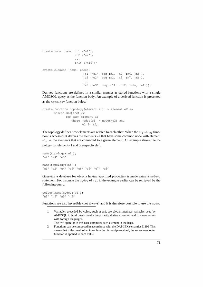
71

create node (name) :n1 (“n1”), :n2 (“n2”), ... :n16 (“n16”);

create element (name, nodes) :e1 (“e1”, bag(:n1, :n2, :n6, :n5)), :e2 (“e2”, bag(:n2, :n3, :n7, :n6)), ... :e9 (“e9”, bag(:n11, :n12, :n16, :n15));

Derived functions are defined in a similar manner as stored functions with a singleAMOSQL-query as the function body. An example of a derived function is presented

as the topology function below1:

create function topology(element e1) -> element e2 as select distinct e2

for each element e2 where nodes(e1) = nodes(e2) and

e1 != e2;

The topology defines how elements are related to each other. When the topology func-tion is accessed, it derives the elements e2 that have some common node with elemente1, i.e. the elements that are connected to a given element. An example shows the to-

pology for elements 1 and 5, respectively2.

name(topology(:e1)); “e2” “e4” “e5”

name(topology(:e5)); “e1” “e2” “e4” “e6” “e8” “e9” “e7” “e3”

Querying a database for objects having specified properties is made using a select

statement. For instance the nodes of :e1 in the example earlier can be retrieved by thefollowing query:

select name(nodes(:e1));“n1” “n6” “n5” “n2”

Functions are also invertible (not always) and it is therefore possible to use the nodes

1. Variables preceded by colon, such as :n1, are global interface variables used byAMOSQL to hold query results temporarily during a session and to share valueswith foreign languages.

1. The “=” operator in this case compares each element in the bags.2. Functions can be composed in accordance with the DAPLEX semantics [119]. This

means that if the result of an inner function is multiple-valued, the subsequent outerfunction is applied to each value.

72

function in the opposite direction which can be expressed as:

select name(e) for each element e where nodes(e) = :n1;“e1”

Deletion of types, functions, and objects is performed through a delete statement as:

delete type element;delete function nodes;delete :e1;

In addition to database population by object creation and attribute assignments it is pos-sible to use function update statements set , add, and remove , and type update state-ments add and remove . Examples of update statements for functions are:

set nodes(:e1) = bag(:n1, :n2, :n6);add nodes(:e1) = :n5;remove nodes(:e1) = :n2;

A more complete presentation of data management capabilities in AMOS andAMOSQL is presented in [9].

4.4 EMBEDDING, INTERFACING AND EXTENDING AMOS

The two basic alternatives for connecting applications to AMOS are either through atight or a loose connection.

In the tight connection, or embedded DBMS connection, AMOS is directly linked to-gether with a C-based application program. Since this means that the application andAMOS are executing in the same address space, it provides the fastest connection pos-sible. By using a driver program in C that initialises AMOS and catches AMOS errors,the DBMS can be linked to the application as a C-library. A possible disadvantage withthis approach is that execution errors in the application may cause AMOS to crash.

For the loose connection, or the client-server connection, the application can work as aclient to an AMOS server. A client-server connection permits that several applicationsaccess the same AMOS server concurrently. In this situation, the application andAMOS are executing in different Unix processes. This approach makes the AMOSserver more resistant to execution errors in the application. If an application crashes, itwill not afflict the AMOS server. The main disadvantage in this approach is the over-head of the inter-process communication. In comparison to the tight connection, the ac-cess time can be several order of magnitudes higher in this loose connection.

For both these types of connections there are two possibilities to communicate with

73

AMOS from the host language of the application; either through the embedded queryinterface or through the fast-path interface. Currently, the host language should be C(or being able to call C), since the interface routines are available in C.

In a tight connection, the embedded query interface, AMOSQL statements can be exe-cuted from the host language by calling an AMOSQL execution procedure that takesstrings of AMOSQL statements as input. After evaluating the AMOSQL statement, itreturns the value of the evaluation as the result. Carrying out the evaluation means thatthe parser and the query processor must be activated for interpreting and executing thestatement.

This can be avoided by using the fast-path interface through which calls to predefinedand preoptimized AMOSQL functions can be made directly, thereby evading the pars-ing and query processing step. It should be noted that using the fast-path, instead of theembedded query interface, is significantly faster. According to [9], the difference is upto two orders of magnitude. The normal database-access from the application shoulduse this technique of defining AMOSQL functions for database-related application op-erations and later invoke them from the application using the fast-path interface.

In addition to the procedure for using the embedded query and fast-path interface, re-spectively, the inter-process communication must be activated when the client-serverconnection should be used.

For transferring data between the host language and the database AMOS uses objecthandles, i.e. logical references to C data structures stored in the database. An operation,termed dereferencing, can convert the object handle into the C pointer that refers to thecorresponding data record. The interface library provides routines for managing datareferenced by object handles, such as primitives for declaring, assigning, deassigning,and dereferencing object handles.

Furthermore, AMOS includes an embedded Lisp interpreter that provides similar capa-bilities (and sometimes simpler) for exchanging Lisp data with the database as was de-scribed for C. There also exist interface routines between C and Lisp.

According to the previous Section 3.2, there were three categories of extensibility thatcould be identified for an extensible DBMS. These were query language, query proces-sor, and storage manager extensions. AMOS is extensible on all these levels.

At the query language level, the user can define application-specific types and opera-tions using AMOSQL. How users can create new types in AMOSQL was described inSection 4.3, that also included examples on how to define operations as AMOSQLfunctions.

It is further possible to seamlessly extend AMOSQL with new database operations by

74

defining AMOSQL functions as foreign and using a conventional programming lan-guage (such as C or Lisp) for their implementation. This is done by means of the foreignfunction interface that allows AMOSQL to communicate with external programminglanguages.

AMOSQL foreign functions can be uni-directional or multi-directional. A uni-direc-tional function is a normal function with the simple intention to compute the result (oneor several) given the values of its arguments. The following example shows how to de-fine a uni-directional function abs , that computes the absolute value of a number usinga foreign Lisp function:

create function abs(number n1) -> number n2 as

foreign abs.number.number;

where abs.number.number is the name of the Lisp function that implements the abs

AMOSQL function. The abs.number.number implementation only includes a call tothe Lisp abs function:

(define abs.number.number (obj osql:n1 osql:n2)

(osql-result osql:n1 (abs osql:n1)))

Like AMOSQL functions, foreign functions can be multi-directional. A multi-direc-tional function is defined, and can be applied, for different binding conditions. Thebinding conditions state the admissible combinations of bound and unbound (free) ar-guments and result variables for a certain function and are defined in a binding pattern,i.e. a list of - (bound) and + (free) symbols. For uni-directional functions, the argumentsare always bound and the results are unbound that state the (- +) binding pattern for theabs function. The reasons for having this multi-directional capability include a reduc-tion of the number of operator signatures that are necessary for a specific amount offunctionality and that the query optimization is enhanced. By reducing the number ofoperations while keeping the functionality will further result in simpler domain modelsand support reusability. To exemplify this capability we show how the minus function

can be implemented by inverting the plus function1.

create function minus(number n1, number n2) -> number n3 as

select n3 where n3 + n2 = n1;

Here, the definition of the minus AMOSQL function reuses the plus multi-directionalforeign function and for different possible binding patterns the correct variant of theplus function will be applied. The definition of the plus function must be made foreach applicable binding pattern. The most obvious ones are those that correspond to one

1. The “+” operator is in-fix syntax for the plus function. Furthermore, the minusand plus functions are actually system-provided functions but are here used in asimple example to include most of the interesting ingredients.

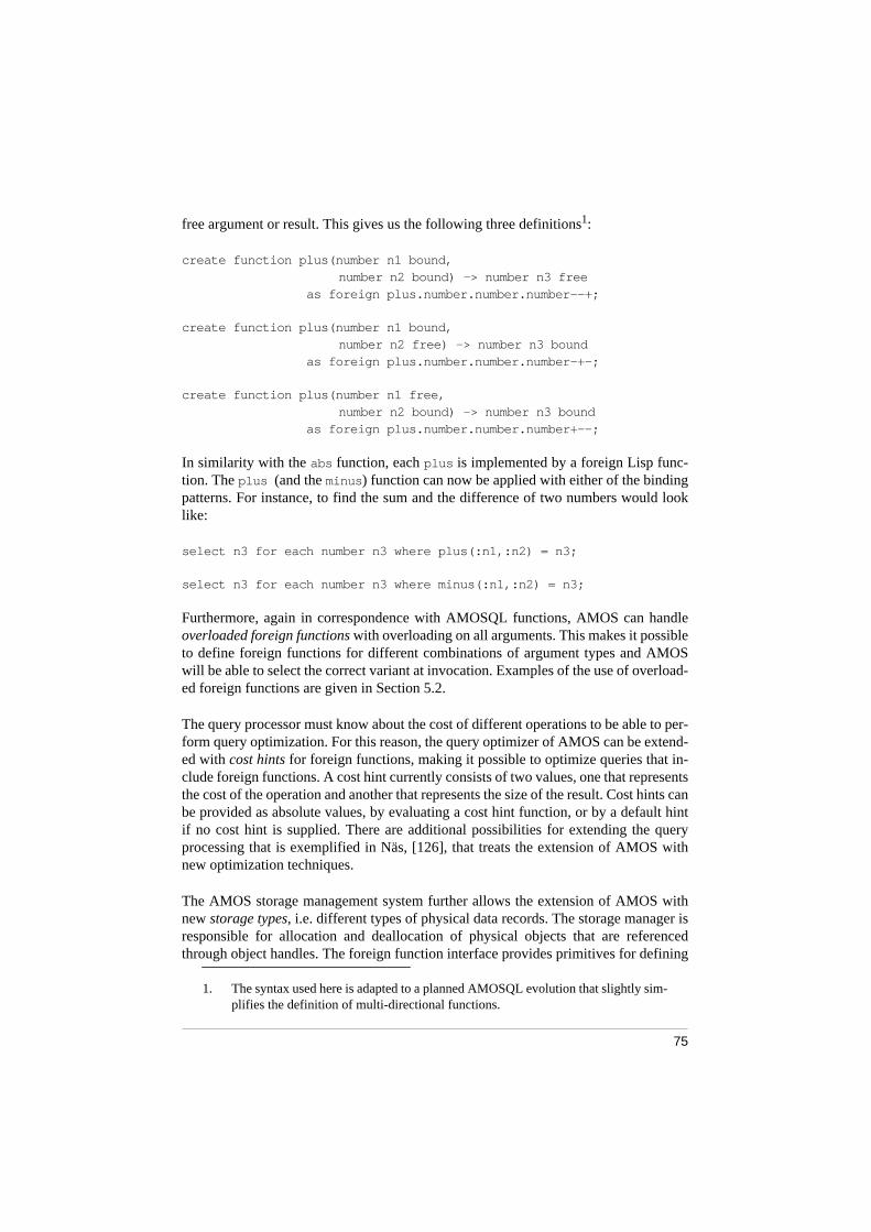
75

free argument or result. This gives us the following three definitions1:

create function plus(number n1 bound, number n2 bound) -> number n3 free

as foreign plus.number.number.number--+;

create function plus(number n1 bound, number n2 free) -> number n3 bound

as foreign plus.number.number.number-+-;

create function plus(number n1 free, number n2 bound) -> number n3 bound

as foreign plus.number.number.number+--;

In similarity with the abs function, each plus is implemented by a foreign Lisp func-tion. The plus (and the minus ) function can now be applied with either of the bindingpatterns. For instance, to find the sum and the difference of two numbers would looklike:

select n3 for each number n3 where plus(:n1,:n2) = n3;

select n3 for each number n3 where minus(:n1,:n2) = n3;

Furthermore, again in correspondence with AMOSQL functions, AMOS can handleoverloaded foreign functions with overloading on all arguments. This makes it possibleto define foreign functions for different combinations of argument types and AMOSwill be able to select the correct variant at invocation. Examples of the use of overload-ed foreign functions are given in Section 5.2.

The query processor must know about the cost of different operations to be able to per-form query optimization. For this reason, the query optimizer of AMOS can be extend-ed with cost hints for foreign functions, making it possible to optimize queries that in-clude foreign functions. A cost hint currently consists of two values, one that representsthe cost of the operation and another that represents the size of the result. Cost hints canbe provided as absolute values, by evaluating a cost hint function, or by a default hintif no cost hint is supplied. There are additional possibilities for extending the queryprocessing that is exemplified in Näs, [126], that treats the extension of AMOS withnew optimization techniques.

The AMOS storage management system further allows the extension of AMOS withnew storage types, i.e. different types of physical data records. The storage manager isresponsible for allocation and deallocation of physical objects that are referencedthrough object handles. The foreign function interface provides primitives for defining

1. The syntax used here is adapted to a planned AMOSQL evolution that slightly sim-plifies the definition of multi-directional functions.

76

this kind of new data storage types. AMOS maintains a global type table with informa-tion about the properties of the built-in physical storage types, such as integer, real,string, object, etc. The introduction of a new storage type is made by expanding the typetable with a new entry with information that includes the type name, size, allocationmethod, deallocation method, and more. In addition, each storage type should have acorresponding C record template that should include type information, a referencecounter, and the data part. This capability can be used to define tailored data structures,required in many scientific and engineering applications, that can be made available inAMOSQL.

The AMOS System Manual [128] treats most of the issues discussed in this section inmore detail. Various aspects of foreign functions are discussed in Litwin and Risch[103], Flodin and Risch [86], Flodin [87], and Flodin et al. [19].

77

5 THE FEAMOS APPROACH

This chapter describes the FEAMOS system in more detail, starting with a recapitulationof the motivation for the approach of using database technology as a basis for implement-ing FEA applications. The next section presents the FEAMOS architecture that showshow the previously presented AMOS architecture is specialised for FEAMOS. The in-ternal architecture shows how the FEAMOS application is designed, which is followedby an illustration of how it fits in a mediator-based EIS environment. After the architec-tural description, there is a section that describes the design and implementation of thematrix and array data sources that extend AMOS with storage structures and operationssuitable for numerical and linear matrix algebra within the database. The subsequent sec-tion describes the current FEA domain model that has been developed for the FEA do-main. The presentation of this high-level FEA domain modelling is divided into subsec-tions that cover specific parts, including: geometry, mesh, boundary, solution algorithm,result interpretation. The final subsection treats performance issues for the current im-plementation status of FEAMOS where comparisons are made with TRINITAS.

The FEAMOS system consists of the TRINITAS FEA application equipped with a localembedded AMOS DBMS linked to the application. By using this approach the applica-tion gains access to general database capabilities tightly coupled to the application it-self. On the external level, this approach facilitates data mediation among applicationsand data sources in the EIS environment. Furthermore, this provides the application in-ternally with complete DBMS capabilities.

78

The basic idea in the FEAMOS approach is to use database technology as a basis fordeveloping the FEA application. In our case, the conventional database approach ofonly storing and accessing data is also extended with the possibility to perform applica-tion-specific operations on data within the database. In this context, we use the termcomputational database technology to provide a vocabulary for referring to databasetechnology that supports applications with a major need for computational support,which is here exemplified by FEA for computational mechanics.

To recapitulate, we have identified certain database technologies that we think are im-portant and suitable as computational database technologies for this task. These keytechnologies are main-memory resident, extensible, and object-relational databasetechnologies in combination with the domain model concept.

Main-memory DBMSs, such as AMOS, are prerequisites for the embedded database ap-proach and to support processing efficiency comparable to that of programming lan-guages.

Extensibility should be provided for the query language, the query processor and thestorage manager. The query language extensibility of AMOSQL provides user-definedtypes and operations and supports powerful means for flexible domain modelling whileletting the DBMS perform data access optimization. AMOSQL also provides extensi-bility of the query optimizer, which permits the introduction of more complex domain-specific cost models that reflect certain aspects of the application domain. For example,costs for numerical operations or solution accuracy of numerical calculations can be in-cluded in the cost models. Thus, the query optimization can influence the choice andtuning of operators in FEA. Furthermore, the AMOS storage manager can be extendedwith tailored data representations that can be specialised for numerical operations orother application-critical tasks.

The term object-relational presupposes the existence of an extensible OO query lan-guage. The AMOSQL query language provides the application with a declarative ac-cess language to the database. A declarative query language in combination with queryoptimization supports high-level modelling with powerful capabilities for data inde-pendence. In addition, AMOSQL has the unique capability of supporting multi-direc-tional functions with overloading on all arguments that extends the modelling capabilityand increases the possibility of reuse. Query languages also make it possible to makeadvanced ad hoc queries concerning the contents of the database. This might be de-manded by advanced users and is quite useful since it is impossible to foresee the com-plete information needs.

These database technologies form the basis for the FEAMOS approach to define do-main models that represent a conceptualisation of the FEA domain and which can takeadvantage of DBMS functionality for its definition, compilation, and optimization.

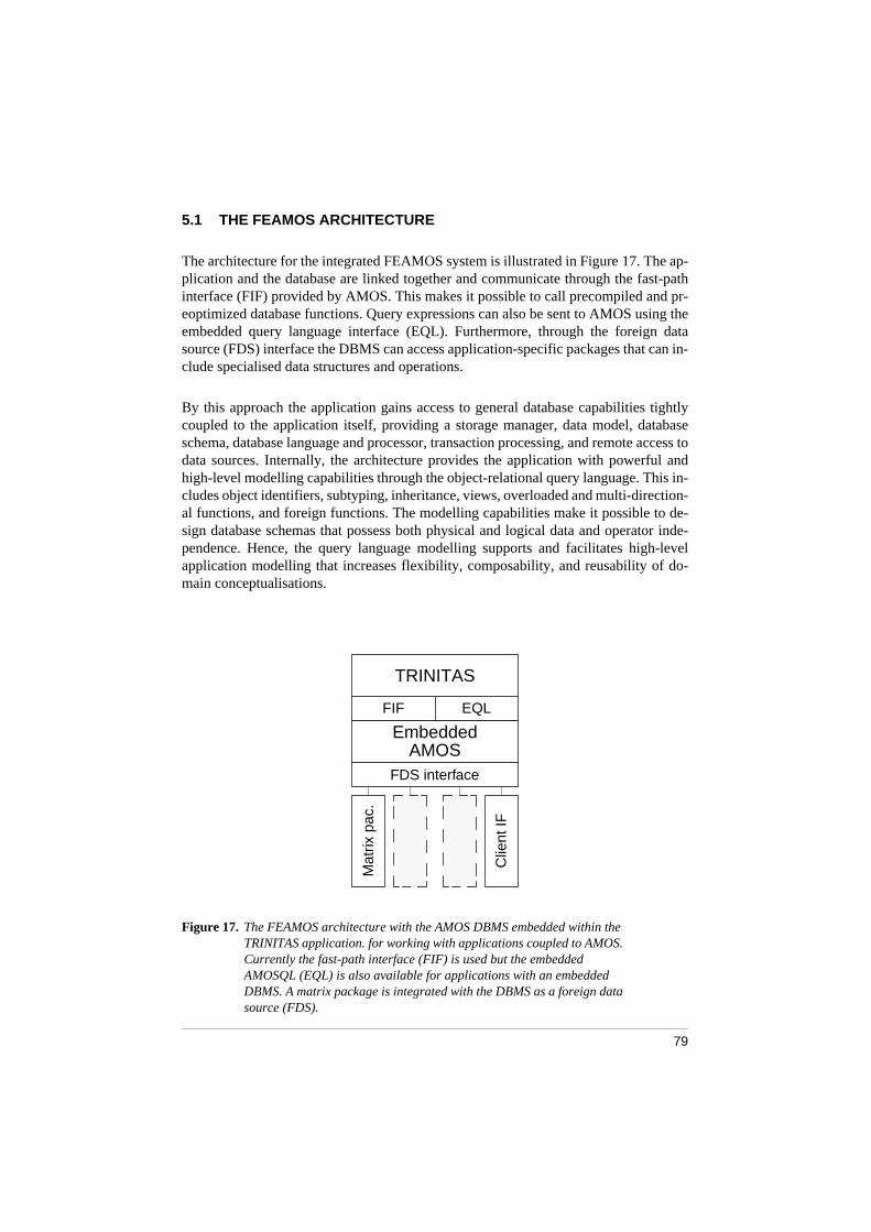
79

5.1 THE FEAMOS ARCHITECTURE

The architecture for the integrated FEAMOS system is illustrated in Figure 17. The ap-plication and the database are linked together and communicate through the fast-pathinterface (FIF) provided by AMOS. This makes it possible to call precompiled and pr-eoptimized database functions. Query expressions can also be sent to AMOS using theembedded query language interface (EQL). Furthermore, through the foreign datasource (FDS) interface the DBMS can access application-specific packages that can in-clude specialised data structures and operations.

By this approach the application gains access to general database capabilities tightlycoupled to the application itself, providing a storage manager, data model, databaseschema, database language and processor, transaction processing, and remote access todata sources. Internally, the architecture provides the application with powerful andhigh-level modelling capabilities through the object-relational query language. This in-cludes object identifiers, subtyping, inheritance, views, overloaded and multi-direction-al functions, and foreign functions. The modelling capabilities make it possible to de-sign database schemas that possess both physical and logical data and operator inde-pendence. Hence, the query language modelling supports and facilitates high-levelapplication modelling that increases flexibility, composability, and reusability of do-main conceptualisations.

Figure 17. The FEAMOS architecture with the AMOS DBMS embedded within the TRINITAS application. for working with applications coupled to AMOS. Currently the fast-path interface (FIF) is used but the embedded AMOSQL (EQL) is also available for applications with an embedded DBMS. A matrix package is integrated with the DBMS as a foreign data source (FDS).

Mat

rix p

ac.

TRINITAS

FIF EQL

EmbeddedAMOS

FDS interface

Clie

nt IF

80

On the external level, this approach supports, among other things, concurrency, inter-operability, data exchange and transformation, data and operator sharing, data distribu-tion among applications and data sources in the EIS environment as illustrated inFigure 18. Different AMOS mediators can be combined for locating, translating, andintegrating data in various data sources for the applications. Ultimately, the DBMS candecide how and where to execute a query, using query optimization techniques. By pro-viding several mediators with the same application package, as illustrated by the matrixpackage in Figure 19, it will be possible to decide where the execution should takeplace.

Figure 18. A mediator-based EIS architecture that illustrates how a combination of different types of mediators (AMOS DBMSs) is used to mediate data among applications and data sources. Each application is equipped with an embedded DBMS.

Figure 18 shows an example of how an EIS environment could be extended with datamanagement capabilities by taking advantage of the mediator approach. Each applica-tion can have its own embedded DBMS (E-AMOS) that can communicate with othermediators. For example, an integrator (I-AMOS) and possible translators (T-AMOS),can support the FEA application to retrieve analysis data that reside in a relational da-tabase (RDB) or in a STEP import file. The CAD application can provide geometric

FEA

E-AMOS

PDM

E-AMOS

NS-AMOS

T-AMOS

RDB

I-AMOS

S-AMOS STEP file

T-AMOST-AMOS

OODB

CAD

E-AMOS

CAx

E-AMOS

81

data through its own mediator to a database server (S-AMOS). An OO database(OODB) can be used for long-term storage of FEA data. A product data management(PDM) system can be used for administrating product data in the EIS system. The nameserver (NS-AMOS) is used to locate where data is stored. The domain models that coverthe different applications are parts of the global schema of the mediator system.

Figure 19. A possible client-server architecture for working with applications coupled to AMOS. The fast-path interface (FIF) and the embedded AMOSQL (EQL) can be used to communicate with the DBMS by applications with an embedded DBMS. AMOS also includes a foreign data source (FDS) interface for integrating foreign data and operator representations.

It is of vital importance for the application to preserve the execution efficiency whileadding functionality to the system. There are several factors that influence the overallperformance in database systems where conventional engineering applications are com-

CIF

AMOSServer

Mat

rix p

ac.

TRINITAS

FIF EQL

EmbeddedAMOS

Mat

rix p

ac.

FDS interface

FDS interface

SIF

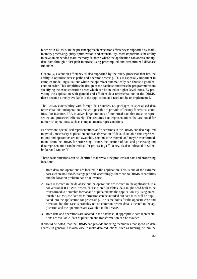
82

bined with DBMSs. In the present approach execution efficiency is supported by main-memory processing, query optimization, and extensibility. Most important is the abilityto have an embedded main-memory database where the application can access and up-date data through a fast-path interface using precompiled and preoptimized databasefunctions.

Generally, execution efficiency is also supported by the query processor that has theability to optimize access paths and operator ordering. This is especially important incomplex modelling situations where the optimizer automatically can choose a good ex-ecution order. This simplifies the design of the database and frees the programmer fromspecifying the exact execution order which can be stated in higher-level terms. By pro-viding the application with general and efficient data representations in the DBMS,these become directly available to the application and need not be re-implemented.

The AMOS extensibility with foreign data sources, i.e. packages of specialised datarepresentations and operations, makes it possible to provide efficiency for critical activ-ities. For instance, FEA involves large amounts of numerical data that must be repre-sented and processed effectively. This requires data representations that are tuned fornumerical operations, such as compact matrix representations.

Furthermore, specialised representations and operations in the DBMS are also requiredto avoid unnecessary duplication and transformation of data. If suitable data represen-tations and operations are not available, data must be moved, and maybe transformed,to and from the DBMS for processing. Hence, the location of data and processing anddata representation can be critical for processing efficiency, as also indicated in Stone-braker and Moore [6].

Three basic situations can be identified that reveals the problems of data and processinglocation:

1. Both data and operations are located in the application. This is one of the extremecases where no DBMS is engaged and, accordingly, there are no DBMS capabilitiesand the location problem has no relevance.

2. Data is located in the database but the operations are located in the application. In aconventional R DBMS, where data is stored in tables, data might need both to betransformed to a suitable format and duplicated into the application. By using an ex-tensible DBMS, the data transformation can be avoided but data must still be dupli-cated into the application for processing. The same holds for the opposite case anddirection, but this case is probably not so common, where data is located in the ap-plication and the operations are available in the DBMS.

3. Both data and operations are located in the database. If appropriate data representa-tions are available, data duplication and transformation can be avoided.

It should be noted, that the DBMS can provide indexing techniques that speed up dataaccess. In general, it is also wise to make data reductions, such as filtering, within the

83

database before data is transferred to the application. Hence, to take full advantage ofthe DBMS capabilities might require that certain parts of the application-specific oper-ations should be performed by the DBMS. If this were solved for existing applications,it might imply a severe redesign of the application logic.

The size and number of data items must also be considered in evaluating where to locatedata and operations. These kind of decisions, of where the processing should take place,could also be supported by the query processor. By defining appropriate cost measuresfor operators at different locations, the execution can directed to the one (or even sev-eral) of the servers in a network that is most cost-effective.

In FEAMOS, a manipulation of an application object through the TRINITAS user in-terface, or by an application procedure, implies an immediate update of the database.For example, when a point is moved on the screen it is a database point object that isupdated. Thus, since application data is only stored in one place, data redundancy andinconsistency can be avoided.

With the availability of the query language it is further possible to query the contents inthe database through the query language interface of the database. For example, we arecurrently using a www-interface in AMOS to connect a www-browser to the DBMS forinteractive query access.

5.2 EXTENDING AMOS WITH LINEAR MATRIX ALGEBRA

One main idea in this work was to provide analysis capabilities in a database environ-ment that can support the needs of scientific and engineering applications. As the usageof database techniques will increase in scientific and engineering disciplines the re-quirements on analysis capabilities will grow. Scientific and engineering applicationsare computationally intensive applications and the idea is to provide numerical analysiscapabilities within the database environment to support the processing needs of theseapplications. The foreign data source for arrays, described in the next section, was de-signed and implemented with the intention to use it for implementing support for nu-merical linear algebra in AMOS.

By providing both data structures suitable for these applications and corresponding op-erations that are relevant it is possible to choose where the data should be located andwhere the processing should take place. Data transportation between the application andthe database that are not required can be eliminated. Further, the types of analysis capa-bilities, together with the proposed architecture described in Section 4.2 and Section5.1, that involve local embedded databases within applications, can provide new pow-erful techniques for developing scientific and engineering applications.

Hence, we would like to have numerical matrices in the database, not only the array datastructure. This makes it possible to perform operations on matrices, producing new or

84

modified matrices, compared to only accessing the physical array data structure. Thereare several research examples of how to provide this functionality in applications usinga conventional approach, i.e. numerical analysis packages in programming languages.This includes both traditional programming languages, such as FORTRAN and C, An-derson et al. [129], as well as OO languages, such as C++, CommonLisp (includingCLOS), OO dialects of Pascal, and Smalltalk, Baugh and Rehak [38], Fenves [39],Forde et al. [40], Filho and Devloo [41], Dubois-Pelerin et al. [42], Williams et al. [43],Scholz [44], Baugh and Rehak [45], Mackie [46], Ross et al. [47], Raphael and Krishna-moorthy [48], Yu and Adeli [49], Hoffmeister et al. [50], Arruda et al. [51], Devloo[52], Eyheramendy and Zimmermann [53], Gajewski [54], Ju and Hosain [55], Shep-herd and Lefas [56], Langtangen [57], Cardona et al. [58], Zeglinski et al. [59], Lu et al.[60], Dongarra et al. [130], Dongarra et al. [131], and Barton and Nackman [132]. Ourapproach shares several ideas with the programming-language approach and further ex-tends the ambitions in terms of expressibility and functionality by providing query-lan-guage integration and database facilities. Likewise, we extend the conventional data-base approach of only storing and accessing data with capabilities for numerical analy-sis within the DBMS. By having matrix types in the database it is possible to extend thequery language with operations on matrices to form an algebra for the matrix domainthat can be used in application modelling. It would further be possible to introduce spe-cial query optimization methods for numerical data processing to support automatic op-timization of execution plans for numerical methods. This could, for instance, includedecisions for selecting a suitable data representation, solution method, and processinglocation.

The need to include data storage types for collections of numerical data in DBMSs hasbeen emphasised by several authors including Sarawagi and Stonebraker [133], Maierand Vance [3], Maier and Hanson [134], Vandenberg and DeWitt [135], Libkin et al.[136], Rotem and Zhao [137], and Seamons et al. [138]. In these works they mainly ad-dress the issue of providing numerical storage types from a secondary-storage perspec-tive. An issue for future work would be to investigate how these techniques could becombined with the approach in this work focusing on main-memory representations.

5.2.1 Linear algebra for finite element analysis

A central problem in the present application domain of FEA is the solution of linearequation systems. This is a characteristic that is shared among many formulations ofscientific and engineering problems. The solution process of linear equations is illus-trated by an example from the FEA domain. First, the multiplication of general matricescan be expressed by the equational relation,

(50)

where matrix A times matrix B is equal to matrix C. If A and B are known and fulfilcertain properties we can calculate C by matrix multiplication. In some cases it is also

A B C=

85

possible to calculate A or B if the two other matrices are known. However, this is notas straightforward as in the former case since it usually involves the solution of somekind of equation system.

A specific case, but central in scientific and engineering computations, is the case whereEq. (50) forms a linear equation system. In this case, the equation system is composedof one square matrix A, and two column matrices b and c.

In the FEA domain, the solution of these types of equation systems is a central issue. Acommon problem in this domain is to solve an equation (stated earlier in Section 2.3 asEq. (30)) of the form

. (51)

Recalling from Section 2.3, that in the treatment of linear elasticity problems, K is usu-ally called the stiffness matrix, a the displacement vector, and f the load vector. Further,in linear elasticity, the stiffness matrix is symmetric and non-singular. If appropriateboundary conditions are enforced and the equations corresponding to fixed displace-ments are eliminated, the resulting submatrix of K will become positive definite.

These types of linear systems are usually solved by transforming the equation systeminto one or several equation systems that are simpler, but equivalent, to solve. In theFEA domain, this process usually involve a decomposition of K into a set of matrices.There are various decomposition methods, but a common method in FEA decomposesK into three matrices as

(52)

where L is a lower unit triangular matrix, D is a diagonal matrix, and U is an upper unittriangular matrix. Unit triangular matrices have unit values in its diagonal. Furthermore,

for non-singular symmetric matrices it holds that U = LT, Golub and van Loan [139].

This decomposition method is called LDLT decomposition, or Crout decomposition.Further, due to the symmetry, this decomposition reduces the amount of computationwork to perform. It can also be computed without engaging the right-hand side of Eq.(51) in contrast to conventional Gauss elimination techniques. Alternative decomposi-tion methods can be added to cover additional problem classes.

Hence, Eq. (51) can be transformed into the equivalent form

. (53)

Now, by introducing the intermediate quantities y and z, Eq. (53) can be solved by,

K a f=

K L D U=

UT

D U a f=

86

(54)

where the first and last equation systems are triangular systems and the mid system is adiagonal system or linear scaling. As we shall see later, Eqs. (54) can be solved in astraightforward manner.

5.2.2 Matrix algebraic concepts

Some matrix algebraic concepts will be introduced where the notation mainly followsthat of Golub and van Loan [139]. The vector space of all m-by-n matrices is denoted

by the m-by-n scalar field , where normally S ∈ R, the set of real numbers. How-ever, due to the computational requirements it might be necessary to extend the typesof matrix representations such that S belongs to one of Z (the set of integers), Rf (the setof four-byte reals), and Rd (the set of 8-byte reals). This means that matrices can haveinteger, float, and double representations. If matrix expressions were to allow mixingmatrix types, this must be taken care of in the definition of matrix operations. This dis-tinction is left out in the subsequent presentation of matrix concepts.

Thus, for a matrix A we have,

, where (55)

Here, aij represents the element of A at row i and column j.

Basic matrix algebraic operations of matrices can now be introduced. The conventionalapproach introduces matrix algebraic operations as functions that take matrices as argu-ments and produce new or altered matrices. Here, a somewhat different approach willbe applied. Since the query language AMOSQL allows the definition of multi-direc-tional functions, it is possible to define operations on matrices as relationships that areisomorphic to the corresponding mathematical expressions. In Golub and van Loan,[139], operations are represented by the notation, where the arrow associates toa one-directional function application. In the present context, this notation is replacedby the notation that is more associated to bi-directional or multi-directional re-lationships. However, it should be noted that this notation does not imply that the rela-tionship exist, or is defined, for every direction that corresponds to the combinations ofmatrix types.

U a y=

D y z=

UT

z f=

Sm n×

A Sm n×∈ A⇔ ai j( )

a11 … a1n

: :am1 … amn

= = ai j S∈

a b→

a b↔

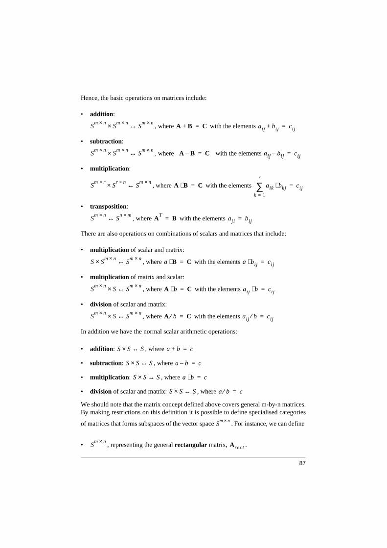
87

Hence, the basic operations on matrices include:

• addition:

, where with the elements

• subtraction:


• multiplication:


• transposition:


There are also operations on combinations of scalars and matrices that include:

• multiplication of scalar and matrix:


• multiplication of matrix and scalar:


• division of scalar and matrix:


In addition we have the normal scalar arithmetic operations:

• addition: , where

• subtraction: , where

• multiplication: , where

• division of scalar and matrix: , where

We should note that the matrix concept defined above covers general m-by-n matrices.By making restrictions on this definition it is possible to define specialised categories

of matrices that forms subspaces of the vector space . For instance, we can define

• , representing the general rectangular matrix, .

Sm n×

Sm n×× S

m n×↔ A B+ C= ai j bi j+ ci j=

Sm n×

Sm n×× S

m n×↔ A B– C= ai j bi j– ci j=

Sm r×

Sr n×× S

m n×↔ A B⋅ C= aik bkj⋅k 1=

r

∑ ci j=

Sm n×

Sn m×↔ A

TB= aj i bi j=

S Sm n×× S

m n×↔ a B⋅ C= a bi j⋅ ci j=

Sm n×

S× Sm n×↔ A b⋅ C= ai j b⋅ ci j=

Sm n×

S× Sm n×↔ A b⁄ C= ai j b⁄ ci j=

S S× S↔ a b+ c=

S S× S↔ a b– c=

S S× S↔ a b⋅ c=

S S× S↔ a b⁄ c=

Sm n×

Sm n×

Arect

88

• , representing a square matrix, , with the same number of rows and

columns.

• , a square matrix with the additional constraint that represents a

symmetric matrix, .

• , a symmetric matrix with the additional constraint for that rep-

resents a diagonal matrix, .

• , a matrix with the same number of rows and columns with the additional

constraint for and that represents an upper triangular matrix,

.

• , an upper triangular matrix with the additional constraint for

that represents an upper unit triangular matrix, .

• , a matrix with the same number of rows and columns with the additional

constraint for and that represents a lower triangular matrix, .

• , an upper triangular matrix with the additional constraint for

that represents a lower unit triangular matrix, .

• , a rectangular matrix with 1 column representing a column matrix, or

.

• , a rectangular matrix with 1 row representing a row matrix type, or .

With these additional categories of matrices, the previous list of matrix operations canalso be specialised further taking the additional categories into account. This is illustrat-ed here for the case of matrix multiplication of rectangular matrices. By identifying in-dex sizes of the arguments and the results the following combinations arise:

• , or matrices categorised as


Sm m×

Asquare

Sm m×

si j sj i=

Asymm

Sm m×

si j 0= i j≠

Adiag

Sm m×

si j 0= i j>

Auptri

Sm m×

si j 1= i j=

Auputri

Sm m×

si j 0= i j< Alowtri

Sm m×

si j 1= i j=

Alowutri

Sm 1×

a

Acol

S1 m×

a Arow

Sm r×

Sr n×× S

m n×↔ Arect Brect⋅ Crect=

Sm n×

Sn n×× S

m n×↔ Arect Bsquare⋅ Crect=

89












Hence, the resulting matrix category of multiplying two (rectangular) matrices is de-pendent on the sizes of the outer indexes of the argument matrices. By interpreting theabove matrix spaces as sub-categories of the rectangular matrix category we get rela-tionships between argument matrix categories and result argument category for the ma-trix multiplication operator. By considering other matrix characteristics, such as sym-metry and singularity, further specialisations of these relationships can be established.For instance, if it is known that a certain matrix is symmetric and it is multiplied withanother matrix, the appropriate result category can be produced. However, if we onlyknow that the matrix is square, the symmetry condition must be evaluated before thisinformation can be used in deciding the result category.

Furthermore, in applications like FEA, it is common to use specialised and more com-pact physical representations, Hughes [23], and Carey and Oden [140], of matrices incontrast to “full” regular matrix representations. As illustrated in Figure 20, there are,for example, skyline matrix (or profile matrix) representations where consecutive zero-valued elements above the “skyline” are left out and the matrix is usually representedby matrix columns in a one-dimensional array. This is an example of a compact repre-sentation where the matrix structure is static, i.e. it is not allowed to change. Additionalstatic representations along the same theme exists. There are also dynamic matrix rep-

Sn n×

Sn m×× S

n m×↔ Asquare Brect⋅ Crect=

Sm 1×

S1 n×× S

m n×↔ Acol Brow⋅ Crect=

Sm n×

Sn m×× S

m m×↔ Arect Brect⋅ Csquare=

Sm m×

Sm m×× S

m m×↔ Asquare Bsquare⋅ Csquare=

Sm 1×

S1 m×× S

m m×↔ Acol Brow⋅ Csquare=

Sm n×

Sn 1×× S

m 1×↔ Arect Bcol⋅ Ccol=

Sn n×

Sn 1×× S

n 1×↔ Asquare Bcol⋅ Ccol=

S1 n×

Sn m×× S

1 m×↔ Arow Brect⋅ Crow=

S1 n×

Sn n×× S

1 n×↔ Arow Bsquare⋅ Crow=

S1 n×

Sn 1×× S

1 1×↔ Arow Bcol⋅ c=

S1 1×

S1 1×× S

1 1×↔ a b⋅ c=

90

resentations where the storage structure is allowed to change. These representationtypes are usually referred to as sparse matrix representations and are typically imple-mented by some linked-list data structure. The categorisations and their usage in estab-lishing the multiplication operator as relationships among different categories that areexemplified above can be further extended to establish relationships between combina-tions of other matrix categories and representations as well as for different operators.

To sum up this part, three principles have been presented that divide the matrix conceptinto different categories, namely:

• mathematically-related matrix categories based on the general matrix concept andits characteristics that further restrict this concept into subcategories.

• the data types, integer, float, and double, used for representing and implementingnumerical matrices.

• various physical representations schemes for representing and implementing matri-ces such as regular, skyline, or sparse. The present representations are restricted tothe regular and skyline type.

Figure 20. Examples of two different one-dimensional physical representations for symmetric and triangular matrices, where X indicates non-zero values. In a), a full storage scheme is illustrated where each element is stored. In the skyline storage scheme, illustrated in b), zeros over the skyline are excluded.

The reason for defining several matrix categories is the potential ability to take advan-tage of the knowledge about specific categories in representing numerical data and ap-

a)

X 0 X 0 X X X X X X 0 0 X 0 XX 0 0 X 0X X X 0

X X XX 0

X

→

b)

X X X X X X X X X 0 XX 0 0 X 0X X X 0

X X XX 0

X

→

skyline

91

plying numerical analysis methods. This concerns the possibilities of applying efficientstorage and processing techniques. So far it is possible to use:

• a priori information to determine matrix categories appropriate for a specific prob-lem.

• information about matrix categories related by a specific operator to determine ap-propriate operator and the correct result (or argument) category.

• information about matrix characteristics, i.e. properties that are not distinguished byseparate categories, to determine correct operator result (or argument) to efficientlydirect subsequent matrix representations and operations.

The next section shows how these matrix concepts can be represented in, and managedby, the AMOSQL extensible and OO query language.

If declarative matrix algebraic expressions do not contain a unique execution order, itis possible to apply some form of operator reordering to obtain an efficient processing.This is analogous to applying query optimization techniques where initial query expres-sions are transformed into equivalent but more efficient execution plans. Optimizationof the execution order for matrix algebraic expressions must be based on the mathemat-ical laws of matrix algebra that restrict the way that these expressions can be trans-formed. In the general case, it should be possible to extend the query optimization tech-niques with capabilities to optimize general query expressions that include matrix alge-braic operators. Similar ideas have been suggested by Wolniewicz and Graefe in [142]for integration of mathematical operations on time series.

For instance, it would be possible to apply the laws for scalar-matrix and matrix-matrixmultiplication, [143], to guide the execution order.

associativity of scalar and matrix multiplication

distributive law of premultiplication

distributive law of postmultiplication

associative law of matrix multiplication

This can be exemplified by the last law, i.e. the associative law of matrix multiplication,that can be expressed in an operator tree as in Figure 21. By using knowledge abouttypes and further matrix properties, a preferred execution order can be decided upon.

c A B( ) cA( )B A cB( )= =

A B C+( ) AB AC+=

B C+( )D BD CD+=

AB( )C A BC( )=

92

Figure 21. Operator trees for the associative law of matrix multiplication where the two trees represent corresponding operations.

The preferred operator order can be determined by comparing the estimated costs cor-responding to operator sequences. This is exemplified by considering the multiplicationof three rectangular matrices. The problem is to find the most efficient execution orderof the following combination of matrix multiplications,

, where . (56)

with the two possible operator sequences that were illustrated in Figure 21. Thus we caneither apply the execution order,

, or (57)

. (58)

The estimated costs for matrix multiplication is proportional to the number of multipli-cations of scalar values that are involved. For a simple matrix multiplication of two rec-

tangular and regular matrices the cost, , can be expressed as:

(59)

where M represents multiplication, m and n is the size of the first matrix and n and k of

the second. Further, , represents a general constant related to the matrix multiplica-

A B C

×

×

CA B

×

×

A B C⋅ ⋅ A Sm n×

B Sn k×

C Sk l×∈,∈,∈

AB( )C

A BC( )

CM

CM CM m n k, ,( ) O mnk( ) C0Mmnk∼= =

C0M

93

tion operator. For combinations of several multiplications we get the total cost, ,

from:

(60)

where the summation is made over i, i.e. all simple multiplication operations. The pre-ferred order can then be found by determining the one with the minimum total cost.

Continuing our example, if we consider as constant over each simple operation, we

can calculate the costs for the two possible execution orders as:

(61)

(62)

where (I) is the case given by (57) and (II) the case in (58). If, for example, we choose

and , we get and . This exam-

ple is illustrated in case a) in Figure 22 and tells us that the first execution order, givenby (58), is preferable. On the other hand, if we choose and

we get and ; pointing out the first execution order, given

by (57), as favourable. This corresponds to case b) in Figure 22.

Instead of calculating actual costs to determine the preferable execution order, one can

use the difference in execution cost, , as the starting point. Hence, we have

. (63)

Since each quantity in Eq. (63) is non-negative, it is possible to state that for

where and,

i) if choose execution order (illustrated by casea) in Figure 22), or

ii) if choose execution order (illustrated by caseb) in Figure 22), or

iii) if the decision is indifferent (exemplified by case c) andd) in Figure 22, or

CtotM

CtotM Ci

M mi ni ki, ,( )i

∑=

C0M

Ctot

MI C0 mnk mkl+( )=

Ctot

MII C0 mnl nkl+( )=

m k 1= = n l 10= = Ctot

MI 20C0= Ctot

MII 200C0=

m k 10= = n l 1= =

Ctot

MI 200C0= Ctot

MII 20C0=

C∆ totM

C∆ totM Ctot

MII Ctot

MI– C0 mn l k–( ) kl n m–( )+( )= =

A B C⋅ ⋅

A Sm n×

B Sn k×

C Sk l×∈,∈,∈

l k–( ) 0> n m–( ) 0>∧ AB( )C

l k–( ) 0< n m–( ) 0<∧ A BC( )

l k–( ) 0= n m–( ) 0=∧

94

iv) if or the decision is indefi-nite and further examinations of the costs must be performed by evaluating the totalcosts measure in (63). This resulting decision can be either of i, ii, or iii. Examplesof this situation are presented in case e) and f) in Figure 22, of which the conclusionin these special cases is that they are indifferent.

Figure 22. Examples of how the execution order and matrix structure affects the cost for consecutive matrix multiplications.

In general, it is preferable to execute contracting operators before expanding operators,but for combined operations the total cost must be considered. Similar preference or-derings can be made for the other multiplication laws and additional operators and op-erator combinations. Furthermore, there are other factors that can affect the executioncost and can be introduced into a cost model, such as the representation scheme andmemory requirements. This last type of optimization technique suggested, cost-basedoptimization of matrix operators, is not yet implemented in the FEAMOS system.

Query optimization can be made both at compile time and at run time. Predefined que-

l k–( ) 0< n m–( ) 0>∧ l k–( ) 0> n m–( ) 0<∧

b)a)

× ×××

d)c)

× ×××

e)

××

f)

× ×

95

ries can be optimized at compile time if the necessary information is available whereasad hoc queries must be optimized at run time. Since query optimization normally is anexpensive operation, it is preferably to perform it at compile time if possible. For exam-ple, the join operation is a commutative operation that results in an exponential increasein possible query plans when several join operations are combined.

It is further possible to use information available at compile time, e.g. type informationor other problem-specific knowledge (such as that the linear-elastic stiffness matrix issymmetric and non-singular), to guide optimization of matrix expressions at compiletime. The type system can be used to select the correct execution plan as long as it isunique, and this is the technique currently being used for solving linear equations.

Since data is not static, conventional query optimization normally uses statistics aboutdata, such as table sizes and predicate selectivities for performing optimization at com-pile time. In analogy with this type of query optimization, it would be possible in thematrix domain to store statistics about average matrix sizes and later apply this knowl-edge in query optimization and compilation to select efficient execution methods. Theapplicability of this technique must be further investigated.

To be able to explore actual sizes and structures of matrices, properties that vary fromone analysis case to another, the optimization must take place at run time. If there are afew possible execution plans or other simple decisions to be made this might be satis-factory with respect to efficiency. For instance, the associative law of matrix multipli-cation, considered in the former example, represents a lower combinatorial complexitythan the commutative relational join operation that has factorial complexity. For facto-rial complexity we have:

, where , according to Stirling’s formula [144].

In the case of the associative law of matrix multiplication we have:

.

Hence, matrix multiplication exhibits a lower exponentiality than the join operation.This can indicate that matrix expressions of reasonable size that include a small numberof alternative execution plans, or simple decisions, could be optimized at run-time. Be-fore any further conclusions can be made, additional investigations must be made in thismatter.

However, if run-time optimization is not satisfactory, dynamic optimization can be ap-plied, Cole and Graefe [145], that handles precompiled alternative execution plans. Byprecompiling several alternative execution plans, a specific execution plan can be se-

an n!= n! n ne---

n∼

an 1 3

2 2----------–

1 2–( )n 2–

1 3

2 2----------+

1 2+( )n 2–

+=

96

lected at run time at a much smaller cost than if pure run-time optimization was re-quired.

5.2.3 The matrix foreign data source

If matrix algebraic operators are integrated within the query language it is possible toperform numerical analysis expressed as declarative queries. The query language thenneeds to be extended with:

• A set of basic matrix types and

• A set of basic matrix operations.

It is then possible to use the built-in capabilities of the query language to:

• Perform domain modelling and manipulation where domain concepts are based onmatrix types. Hence, physical conversion between the application and the database,such as copying and transformation of data, can be avoided since the same physicalformats can be supplied at both locations. Having domain concepts in the databaserepresentation that are isomorphic to application concepts also avoids unnecessaryconceptual conversions between concepts in the application and in the database.

• Make queries that involve matrices in combination with other types of data, i.e. que-ries can be stated that combine and process matrix data with other data types (heter-ogeneous data in general). A uniform representation and access to matrix data willalso facilitate the combination of matrix-based data across application boundaries.

• Express composite, and more complex, matrix operations in terms of the basic setof matrix operations. Further, algorithms can be expressed in a data independentmanner in terms of these basic or composite operations. For instance, multi-direc-tional operations can provide reuse of operations, which results in concise algorithmrepresentations.

• Declarative expressiveness can leave execution order decisions to the query proces-sor. Matrix types can be used to control processing of matrix operations. Matrix op-erations can be made polymorphic such that the choice of a specialised and appro-priate algorithm is dependent on the problem type. By having specialised storageschemes and operators for different matrix types it is possible to guide the numericalcomputation into efficient processing alternatives and to choose optimized storageand processing techniques where possible.

• The query processor can be extended to understand domain-specific operators (que-ries) that provide algorithm-choices based on cost measures. Hence, the applicationdomain can take advantage of algebraic and cost-based optimization of matrix, orother, domain operations.

Furthermore, one would like to have appropriate database representations of matriceswith respect to storage and processing concerns. Tailored storage schemes and algo-

97

rithms to optimize storage and processing requirements are common in FEA. For thesereasons, it would be convenient to exploit matrix characteristics based on mathematicalproperties including structure, physical matrix representation schemes, and basic datatypes.

To accomplish the above functionality, it is required (or at least most facilitating) thatthe query language is equipped with certain capabilities. These include:

• Object-oriented features such as user types, subtyping, inheritance, etc., as stated inSection 3.3.1. Object-orientation provides facilities for structuring the matrix do-main in a problem-oriented fashion while reusing specifications in the type taxono-my. The type system also provides the capability to optimize processing by selectingalgorithms based on type information.

• Overloading is required to be able to define variants of matrix operations specialisedfor matrix sub-categories or matrix representations.

• Overloading on all arguments makes it possible to have functions specialised forcombinations of matrix types that is typically the case for matrix operations.

• Multi-directional functions provide the ability to apply functions in multiple direc-tions, facilitating reuse of functions and compact representations.

• Foreign functions are a basic capability for transparently integrating matrix opera-tions within the query language while implementing numerical matrix operations ef-ficiently in a programming language.

• Customized internal data representations are, together with foreign functions, re-quired to be able to handle the representation and processing of specialised matrixrepresentation schemes.

• To be able to direct decisions concerning execution order, selection of redundant al-gorithms, and others, to the query processor, cost-based optimization must be sup-ported.

• Main-memory DBMS technology provides efficient processing capabilities that arevital for numerical analysis computations as performed in FEA.

• Support of integration, combination, and exchange of data from other DBMSs.

In these issues, there are several problems that need to be solved. In pure object-orien-tation only the receiver of a message, corresponding to the first argument of a function,is used for deciding the appropriate method to apply. This is not sufficient to conven-iently define mathematical operations, such as matrix algebraic operations, since oper-ations need to be defined for different combinations of argument types in a type hierar-chy. For example, we can define plus (+) and times (*) for different combinations ofnumbers and matrices as:

plus(number n1, number n2) -> number n3plus(matrix m1, matrix m2) -> matrix m3

98

times(number n1, number n2) -> number n3times(number n1, matrix m1) -> matrix m2times(matrix m1, number n1) -> matrix m2times(matrix m1, matrix m2) -> matrix m3

We see that for the plus function it is sufficient with overloading on the first argumentto be able to distinguish between the two variants. In the other case, where the times

function is overloaded, a selection mechanism based on the first argument is not suffi-cient since there are several possible functions to choose among.

However, there are several examples where matrix class libraries are defined in OO pro-gramming languages like C++, Scholz [44], Ross et al. [47], Yu and Adeli [49], Zeglin-ski et al. [59], Lu et al. [60], Dongarra et al. [131], and Barton and Nackman [132].

These types of languages1 do not permit an automatic treatment of overloading of op-erations on multiple arguments and the operation dispatch must be handled explicitly.An alternative solution would be to have special operators for each case and by provid-ing overloading on all arguments this can be achieved, Flodin et al. [19]. In comparisonto pure object-orientation this technique extends the capabilities for abstraction and re-use.

Furthermore, it would be desirable to be able to apply matrix operations in different di-rections in queries and functions. A simple case is seen in the definition of a matrixtransposition function in the example below

create function transpose(lower_triangular_matrix ltm) -> upper_triangular_fmatrix utm as

select utm where transpose(utm) = ltm;

where transposition of a lower_triangular_matrix is accomplished by applying theinverse of transposing an upper_triangular_fmatrix .

The ability to handle multi-directional functions provides several advantageous fea-tures:

• multi-directional functions make it possible to reuse operations. An example of howthis is applied for reusing matrix operations is given below. The minus operator, inthe example, is expressed in terms of a formerly defined plus operator. In this exam-ple, the first argument of the plus function is unbound and the appropriate applica-tion of the multi-directional plus function will be handled by the system.

create function minus(matrix m1, matrix m2) -> matrix m3 as select a3 where plus(m3,m2) = m1;

• multi-directional applicability of functions can significantly reduce database search,

1. C++ can handle overloading on all arguments if late binding does not occur.

99

reported in Flodin [87]. Multi-directional functions and indexes increase the physi-cal data independence since the system can efficiently execute a function in its mostefficient direction independently from its logical usage.

• multi-directional functions can increase the readability and simplify the applicationdesign since the problem description becomes more domain-oriented and imple-mentation independent.

The following example shows how the solution of a triangular equation systems can beexpressed in a straightforward and mathematically-oriented manner. A triangular equa-tion system is composed by multiplying a triangular matrix and a column matrix; form-ing a second column matrix. This can be expressed by the multiplication function,times, that is overloaded for different types of triangular matrices illustrated by

where the first matrix represents a generic triangular matrix category that has severalspecialisations that correspond to the following multiplication operations:

(64)

There are additional variants of these operations since the matrix categories can havedifferent representation schemes and basic numerical data type. In AMOSQL, the mul-tiplication operators are implemented as multi-directional foreign functions that are de-fined for appropriate binding patterns. A binding pattern is a unique pattern that stateswhich of the interface variables of a function are presumed to be bound and which thatare free (unbound). The current implementation of the times function include the fol-lowing two binding patterns. The first is

(65)

where indexes represent if the function variable is bound (b) or free (f). Here, the twoarguments are bound and the result is free. This binding pattern corresponds to normalmultiplication. Further, operations that correspond to the second binding pattern,

(66)

are not always defined. However, when the second argument is a column matrix, it cor-responds to the solution of different types of linear equation systems (including trian-gular systems). Here the first argument and the result are bound and the second argu-

Sn n×

Sn 1×× S

n 1×↔

Auptri Bcol⋅ Ccol=

Auputri Bcol⋅ Ccol=

Alowtri Bcol⋅ Ccol=

Alowutri Bcol⋅ Ccol=

Ab

Bb⋅ C

f=

Ab

Bf⋅ C

b=

100

ment is free, i.e. the unknown in the equation. The multiplication operators that are cur-rently implemented are listed in Appendix C.

By defining overloaded foreign functions for different binding patterns, the number ofoperations that are required for expressing the same functionality can be reduced. Thesame operation can be reused in application design in a uniform and compact fashion.Furthermore, operations such as matrix algebraic operations can be expressed in amathematically tractable syntax. For instance, all of the operations that correspond toEqs. (64) for solving triangular equation systems form a subset of all the operations thatcan be expressed by the same AMOSQL expression as,

select b for each column_matrix b where :A * b = :c;

where :A and :c are variables bound to matrix OID:s. Defining and composing variousmatrix operations to form more complex expressions that will be executable by the que-ry processor is also allowed. The following query includes a transpose function that willinfluence the decision of which multiplication operator to apply.

select b for each column_matrix b where transpose(:A) * b = :c;

If :A is bound to an upper triangular matrix, the transpose operator will change the typeof :A to a lower triangular matrix and another multiplication operator will be appliedthan if the transpose operation were absent.

As an example of how overloaded multiplication functions can be defined and used weconsider the first and third equation in Eqs. (64). The first equation can be interpretedas corresponding to a matrix multiplication when A and B are known, and to solving anupper triangular linear equation system when A and C are known. For the situationwhere B and C are known the equation has no unique solution. This interpretation canbe captured by overloading a function for matrix multiplication of an upper triangularmatrix with a column matrix that results in another column matrix. This function shouldbe overloaded on the bbf binding pattern and for the bfb binding pattern. By leaving outthe fbb binding pattern, the result will be undefined for this case. This can be defined inAMOSQL by the following two functions.

create function times(upper_triangular_matrix uptri bound, column_matrix cola bound) -> column_matrix colr free as

foreign times.uptri.col.col--+fn;

create function times(upper_triangular_matrix uptri bound, column_matrix cola free) -> column_matrix colr bound as

foreign times.uptri.col.col-+-fn;

In this case, the actual behaviour is implemented by foreign functions in Lisp and C.

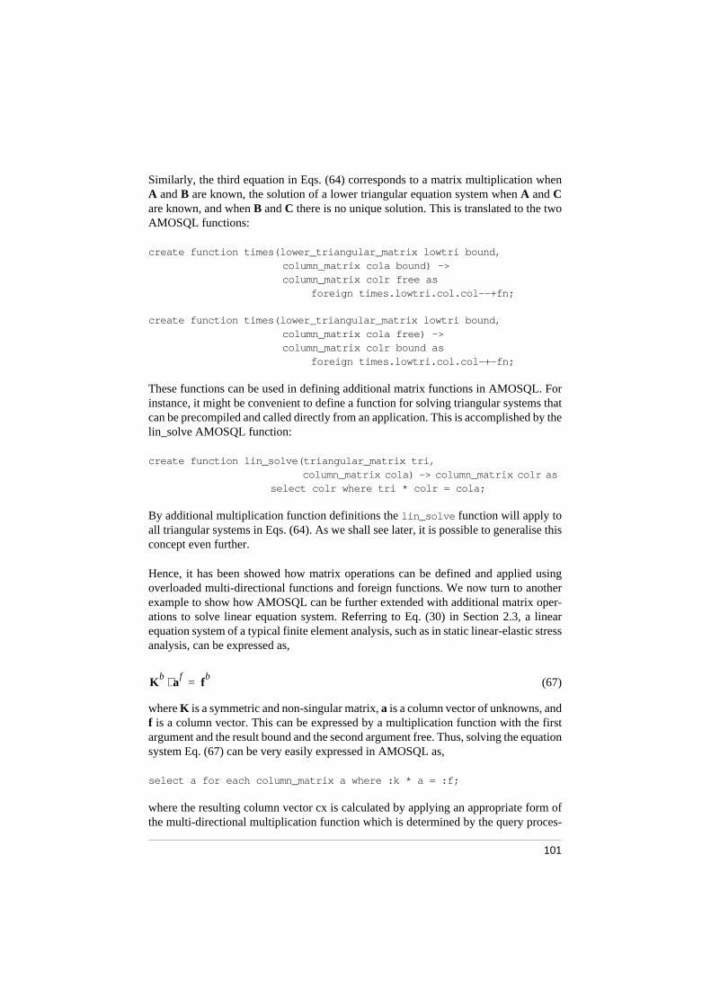
101

Similarly, the third equation in Eqs. (64) corresponds to a matrix multiplication whenA and B are known, the solution of a lower triangular equation system when A and Care known, and when B and C there is no unique solution. This is translated to the twoAMOSQL functions:

create function times(lower_triangular_matrix lowtri bound, column_matrix cola bound) -> column_matrix colr free as

foreign times.lowtri.col.col--+fn;

create function times(lower_triangular_matrix lowtri bound, column_matrix cola free) -> column_matrix colr bound as

foreign times.lowtri.col.col-+-fn;

These functions can be used in defining additional matrix functions in AMOSQL. Forinstance, it might be convenient to define a function for solving triangular systems thatcan be precompiled and called directly from an application. This is accomplished by thelin_solve AMOSQL function:

create function lin_solve(triangular_matrix tri, column_matrix cola) -> column_matrix colr as

select colr where tri * colr = cola;

By additional multiplication function definitions the lin_solve function will apply toall triangular systems in Eqs. (64). As we shall see later, it is possible to generalise thisconcept even further.

Hence, it has been showed how matrix operations can be defined and applied usingoverloaded multi-directional functions and foreign functions. We now turn to anotherexample to show how AMOSQL can be further extended with additional matrix oper-ations to solve linear equation system. Referring to Eq. (30) in Section 2.3, a linearequation system of a typical finite element analysis, such as in static linear-elastic stressanalysis, can be expressed as,

(67)

where K is a symmetric and non-singular matrix, a is a column vector of unknowns, andf is a column vector. This can be expressed by a multiplication function with the firstargument and the result bound and the second argument free. Thus, solving the equationsystem Eq. (67) can be very easily expressed in AMOSQL as,

select a for each column_matrix a where :k * a = :f;

where the resulting column vector cx is calculated by applying an appropriate form ofthe multi-directional multiplication function which is determined by the query proces-

Kb

af⋅ f

b=

102

sor. Looking at this in more detail, the definition the multiplication function for thisbinding pattern involves the application of three additional and simpler multiplicationoperators and a factorisation operator that forms the complete solution of a linear equa-tion system. Again referring to Eqs. (52), (53), and (54) in this section, this solutionprocess can be declaratively expressed by functions corresponding to the equational ex-pressions,

(68)

where U is an upper unit triangular matrix, D is a diagonal matrix, and x and y are col-umn vectors. When K and f are known, the execution order is implicitly given from thebinding patterns. Hence, by defining the operation corresponding to Eq. (67) as the so-lution of Eq. (68), the solution of the a linear equation system can be expressed as theinverse to a single matrix multiplication expression. The query processor will then au-tomatically transform expressions of the form in Eq. (67) to a corresponding represen-tation in Eq. (68). This means that the function for multiplying a symmetric matrix witha column matrix has a straightforward implementation for the bbf binding pattern as,

create function times(symmetric_matrix k bound, column_matrix a bound) -> column_matrix f free as

foreign times.sym.col.col--+fn;

where times.sym.col.col--+fn is the foreign function that should be executed. Forthe bfb binding pattern we should express the transformation of Eq. (67) to Eq. (68)which is accomplished by the following function definition:

create function times(symmetric_matrix k bound, column_matrix a free) -> column_matrix f bound as select a

for each upper_unit_triangular_matrix u, diagonal_matrix d, column_matrix ca, column_matrix cf

where factorise(k) = <u,d> and transpose(u) * cf = f and d * ca = cf and u * a = ca;

Kb

UT( )

fD

fU

f⋅ ⋅=

Ub

af⋅ x

b=

Db

xf⋅ y

b=

UT( )

by

f⋅ fb

=

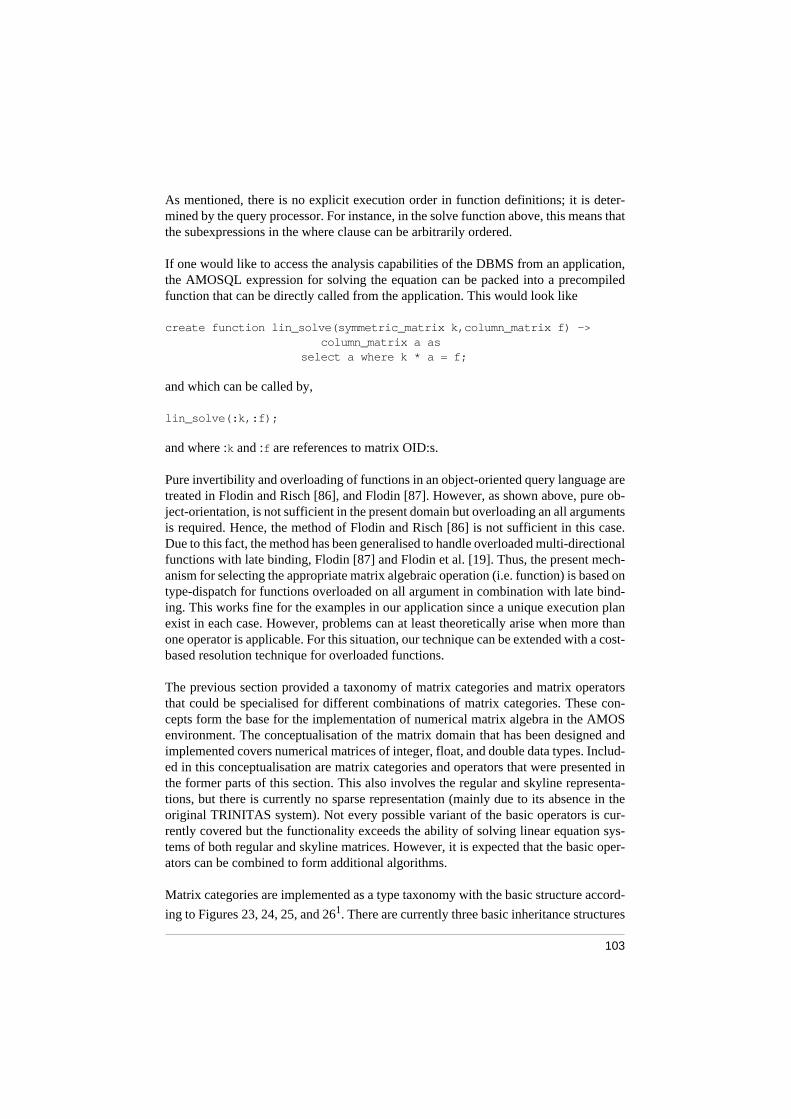
103

As mentioned, there is no explicit execution order in function definitions; it is deter-mined by the query processor. For instance, in the solve function above, this means thatthe subexpressions in the where clause can be arbitrarily ordered.

If one would like to access the analysis capabilities of the DBMS from an application,the AMOSQL expression for solving the equation can be packed into a precompiledfunction that can be directly called from the application. This would look like

create function lin_solve(symmetric_matrix k,column_matrix f) -> column_matrix a as select a where k * a = f;

and which can be called by,

lin_solve(:k,:f);

and where :k and :f are references to matrix OID:s.

Pure invertibility and overloading of functions in an object-oriented query language aretreated in Flodin and Risch [86], and Flodin [87]. However, as shown above, pure ob-ject-orientation, is not sufficient in the present domain but overloading an all argumentsis required. Hence, the method of Flodin and Risch [86] is not sufficient in this case.Due to this fact, the method has been generalised to handle overloaded multi-directionalfunctions with late binding, Flodin [87] and Flodin et al. [19]. Thus, the present mech-anism for selecting the appropriate matrix algebraic operation (i.e. function) is based ontype-dispatch for functions overloaded on all argument in combination with late bind-ing. This works fine for the examples in our application since a unique execution planexist in each case. However, problems can at least theoretically arise when more thanone operator is applicable. For this situation, our technique can be extended with a cost-based resolution technique for overloaded functions.

The previous section provided a taxonomy of matrix categories and matrix operatorsthat could be specialised for different combinations of matrix categories. These con-cepts form the base for the implementation of numerical matrix algebra in the AMOSenvironment. The conceptualisation of the matrix domain that has been designed andimplemented covers numerical matrices of integer, float, and double data types. Includ-ed in this conceptualisation are matrix categories and operators that were presented inthe former parts of this section. This also involves the regular and skyline representa-tions, but there is currently no sparse representation (mainly due to its absence in theoriginal TRINITAS system). Not every possible variant of the basic operators is cur-rently covered but the functionality exceeds the ability of solving linear equation sys-tems of both regular and skyline matrices. However, it is expected that the basic oper-ators can be combined to form additional algorithms.

Matrix categories are implemented as a type taxonomy with the basic structure accord-

ing to Figures 23, 24, 25, and 261. There are currently three basic inheritance structures

104

that rely on multiple inheritance to provide the intended functionality to concrete types.The representation of the three numerical data types are currently modelled by explicittypes, illustrated in Figure 25. In future developments it would be possible (dependenton execution overhead) to treat these representations implicitly by the use of type tem-plates in a similar way to C++, [146]. Then int, float, and double could share the storagemethod and the right data type is accomplished implicitly by casting at access time. Thetype structure that represents mathematical concepts, illustrated in Figure 23, have fur-ther been separated from the matrix representation schemes that have their own typestructure, illustrated in Figure 24. A similar separation is suggested by Chambers andLeavens [147].

Figure 23. The current type taxonomy for representing the mathematical matrix categories.

All matrix types are currently based on one of the numerical array types, described in

1. The type names in the figures have been shortened in some case and the illustrationof the type taxonomy has been slightly compacted for facilitating the overview. Thecomplete type taxonomy can be studied in Appendix B.

square column row

upper tri. lower tri.

rect. matrix

triangularsymmetric

diagonal

lower unit tri.upper unit tri.

105

Section 5.2.4, for their physical representation. They are further implemented as lineararrays, applying a column-order storage sequence. Multiple inheritance is also used forinheriting basic properties from the array types.

As the needs are extended, the type taxonomy can be extended to handle additional rep-resentation schemes and data types as indicated for a sparse representation scheme inFigure 24. It should be noted that it might also be suitable to extend the type taxonomyto handle additional mathematical matrix categories as well. For instance, when the do-main is extended with additional problem categories it can be necessary to distinguish-ing between matrices that are positive definite, positive semi-definite, etc. Whether thetreatment of additional matrix properties should be accomplished by additional sub-types or by another mechanism must be further investigated.

Figure 24. The type taxonomy for representing numerical matrix representation schemes. Regular and skyline matrix schemes are currently implemented, whereas the sparse scheme indicated are not at present included.

Figure 25. The type taxonomy for numerical matrix data types where there are subtypes for integer, float, and double data types of numerical data. The concrete representations are inherited from the corresponding numerical

skyline matrixregular matrix sparse matrix

matrix scheme

float matrixinteger matrix double matrix

matrix type

106

array type that are currently used for the physical representation of all matrix types.

The properties and operations in the matrix domain are implemented by means ofAMOSQL functions. Basic matrix operations that are not specific to matrices are inher-ited from other supertypes, such as array types. An example is the size function that isdefined for the array type. Functions are further multi-directional where it is applicable.The name function can, for instance, be used for retrieving matrix names or for retriev-ing matrices with a given name. There are also several variants of some functions dueto overloading on different function signatures. This is not revealed in the subsequentlist of functions. A more complete list of overloaded foreign functions can be found inAppendix C.

• construct(charstring typename, vector settings) -> boolean

• initialise(matrix mat, vector settings) -> booleanThe initialise function is used for specifying initialisations specific to matrices andis applied by the generic construct function.

• destruct(object obj) -> booleanThe destruct function implements specific matrix behaviour that should be appliedwhen a matrix is destructed by the generic destruct function.

• name(matrix mat) -> charstring aname The name function is a stored attribute that is used for user-defined naming of ma-trices.

• size(matrix mat) -> integer asize The size function derives the size of the matrix that was set at creation time.

• rows(matrix mat) -> integer nrowsThe number of rows of the matrix is held by the stored function rows.

• columns(matrix mat) -> integer nrcolsThe number of columns of the matrix is held by the stored function columns.

• ref(matrix mat, integer indexi, integer indexj) -> number value Matrix elements can be referenced by the ref function where the second and thirdargument specify the indexes of the element that should be determined.

• set(matrix mat, integer indexi, integer indexj, number value) -> booleanThe set function is used for updating matrix elements.

• plus(matrix m1, matrix m2) -> matrix m3 The plus function is a multi-directional function that implements invertible matrixaddition. Alternatively to the prefix notation, the “+” operator can be used in infixnotation.

• minus(matrix m1, matrix m2) -> matrix m3

107

The minus function is a multi-directional function that implements invertible matrixsubtraction. Alternatively to the prefix notation, the “-” operator can be used in infixnotation. Subtraction is defined as the inverse of plus, i.e. the code that implementsplus is reused for the minus function.

• times (matrix m1, matrix m2) -> matrix m3 The times function is a multi-directional function that implements invertible matrixmultiplication. Alternatively to the prefix notation, the “*” operator can be used ininfix notation. Multiplication is overloaded on different function signatures to im-plement efficient operations and for code reuse.

• quotient (matrix m1, number n) -> matrix m2 The quotient function is a multi-directional function that implements invertible ma-trix division where applicable. Alternatively to the prefix notation, the “/” operatorcan be used in infix notation. Currently, the quotient function is not used in the ap-plication.

108

Figure 26. The composite type taxonomy for the matrix domain with individual inheritance structures for the three basic categorisation principles.

• transpose(matrix m1) -> matrix m2 Transposition of matrices that does not do any physical reorganisation, it only cre-ates a new object with a different type without copying data.

• factorise(symmetric_matrix m1) -> <upper_unit_triangular_matrix m2,diagonal_matrix m3> Factorise implements decomposition of symmetric matrices. Furthermore, it is cur-rently implicitly assumed that matrices are nonsingular. Currently the factorise

function implements LDLT decomposition (or Crout decomposition) that divides a

matrix

row vector

column vector

square

symmetric

diagonal

triangular

upper triangular

upper unit triangular

lower triangular

lower unit triangular

matrix scheme

regular

skyline

sparse

matrix representation

imatrix

fmatrix

dmatrix

symmetric skyline imatrix

symmetric skyline dmatrix

symmetric skyline fmatrix

109

symmetric matrix C into three matrices L, D, and U, where L * D * U, L = trans-pose(U), U is an upper unit triangular matrix, D is a diagonal matrix. Here, only Dand U are generated.

• dindex(skyline_matrix m) -> iarray aThe dindex function stores the diagonal index of a skyline matrix to be used by otheroperations for locating specific columns.

Other operators can be expressed in terms of these basic matrix operators, and of course,the current set of base operators can be extended. As an example of the former, a linearcombination of matrices can easily be expressed using the AMOSQL infix notation as,

select m3 for each matrix m3where :a * m1 + :b * m2 = m3;

where :a and :b are reals and :m1 and :m2 are matrices, or by function composition us-ing prefix notation:

select m3 for each matrix m3where plus(times(:a,:m1), times(:b,:m2)) = m3;

This expressibility is accomplished by overloading the times operator on combinationsof number and matrix. Further, expressing this as a function would look like

create function linear_combination(real a, matrix m1, real b, matrix m2) -> matrix as

select a * m1 + b * m2;

5.2.4 The array foreign data source

Many scientific and engineering applications involve one- or multi-dimensional se-quences of numerical data expressing arrays or matrices of numerical values. These areusually used to represent different mathematical concepts, such as scalar-, vector-, ordyadic-valued quantities. Thus, the ability to represent and do computations on se-quences of numerical data is of great importance for scientific and engineering softwaretools. Several commercial “tool kits” for scientific and engineering computations, like

MATLAB 1, MATHCAD2, and HiQ3, support these facts.

Likewise, the database community has emphasised the ability to represent sequences ofnumerical data. This capability can, for instance, be found in commercial products like

Illustra [6] and eBASE4. It has also been developed for research DBMSs including EX-

1. MATLAB is a product of MathWorks, Inc.2. Mathcad is a product of MathSoft, Inc.3. HiQ is a product of National Instruments, Inc.4. eBASE is a product of Universal Analytics, Inc.

110

ODUS [99]. Furthermore, the standard proposals of SQL3 [16] and OQL [17] includedata structures for numerical sequences in their object model. By providing data struc-tures for numerical sequences in a database environment it will be possible to combinethis type of numerical data with other data types, such as simple integer and real numberdata, character strings. Hence, an extended set of data structures are made available forfacilitating modelling and manipulation of the rich set of scientific and engineering da-ta.

In this work, the AMOS object-relational DBMS has been extended with a numericalarray data structure. At the query language level, three different numerical and one-di-mensional, or linear, array types have currently been defined and implemented. The ar-ray types (or classes) are defined for sequences of integers, floats, and doubles, that aredenoted:

• iarray

• farray

• darray

where iarray, farray, and darray represents a fixed sequence of 4-byte integer numbers,4-byte real numbers, and 8-byte real numbers respectively. These three types areformed in a type structure according to Figure 27 where the array type is a subtype ofthe usertypeobject type.

Eight basic operations have currently been defined for arrays at the query language lev-el:

• construct(charstring typename, vector settings) -> boolean

• initialise(array arr, vector settings) -> boolean

• destruct(array arr) -> boolean

• name(array arr) -> charstring aname

• size(array arr) -> integer asize

• ref(array arr, integer index) -> number value

• set(array arr, integer index, number value) -> boolean

where name is a stored function representing an optional name attribute and size is aforeign function that represents the length of the array. The construct and destruct op-erations are general constructor and destructor procedures for implementation of tai-lored creation and deletion operations. The construct operator takes a name of a typeand a vector of initial settings and creates an object of that type. It then applies the ini-tialise operator, overloaded for different types, that defines specific initialisations forthe created object. Finally, the construct operation returns the newly created and initial-ised object.

111

Figure 27. The type hierarchy for numerical arrays where the array type is a subtype of usertypeobject.

The current implementations of the initialise and the construct functions for objects areas follows:

create function initialise( object obj, type tp, vector settings) -> object as

begin/* type-specific initialisations */result obj

end;

create function initialise ( array arr, type arrtype, vector settings) -> array as

beginallocate(arr, arrtype, settings);set name(arr) = vref(settings, 1);result arr

end;

create function construct( charstring typename,vector settings) -> object obj as

begindeclare type tp;set tp = typenamed(typename);set obj = new_object(tp);initialise(obj, tp, settings);result obj

end;

As an example of how tailored constructor functionality can be accomplished, the sec-ond initialise function above is designed for the array type by overloading the initialisefunction for a corresponding array type signature. The values of the size and name at-

iarray farray darray

iarray

112

tributes are extracted from the settings vector and initiated by the allocate and set oper-ations. More specifically, the allocate operation is responsible for allocating a literal ar-ray object (a basic data storage structure) of a specified size and associating it with anobject of type array. The constructor and destructor operations were mainly introducedto provide tailored creation and deletion for array types and subsequent extensions tomatrices and domain-specific types presented in Section 5.3.3. Parallel work on AMOShas generalised the applicability of constructors to any user-defined type [93]. Similarfunctionality is specified in the SQL3 proposal. The ref and the set operator are foreignfunctions for retrieving and updating single array values. Additional retrieval and up-date operators are required as well, but these are still provided by the FEA application.This includes operators for accessing subparts of an array and similar operations on oth-er aggregation data structures based on arrays. Operations of this type are not normallysupported in array representations for databases but are of great importance to engineer-ing applications and are supplied in “tool-kits” such as MATLAB and others. As wehave seen in the previous section, this basic array type structure is further extended byadding subtypes of arrays and by adding operators that are required in specific applica-tions.

Below the query language level, the new array data source is defined by a literal arraydata type. The array data type is complemented by a set of basic operations that are ac-cessible from both LISP and C. Foreign functions, defined at the query language level,are defined by means of operations at this level that operate on literal arrays. Since it ispossible to dereference the array data structure from the literal object, it is possible toimplement critical and kernel array operations as efficiently as in conventional pro-gramming languages.

Hence, as described in Section 4.4, C record templates for the literal array data types aredefined for iarray, farray, and darray. The techniques for defining and registering newstorage data types that were described in the same section have been used. An exampleof the record template for the farray data type (float array) is provided below.

struct farray{ objtags tags;

char filler1[2];int len;char filler2[4];char cont[sizeof(float)];};

The objtags include type information and reference counters for storage management,len is the size of the array, and the last. char declaration is a pointer to the data seg-ment. The basic data structure is of the same type as arrays in C and Fortran.

There are currently five basic operations defined on literal arrays which are implement-ed in C. Here, they are exemplified for float arrays:

• mkfarrayfn(arraysize) creates a literal float array object where the number of ele-

113

ments is determined by arraysize.

• farraysizefn(array) retrieves the size of the literal array object.

• farrayreffn(array, arrayel) retrieves the value of the float, in the literal array object,at the position determined by index.

• setfarrayfn(array, arrayel, elvalue) assigns the float value to the float, in the literalarray object, at the position determined by index

These operations are all implemented in C. They are also registered to LISP using astandardised naming convention and are accessed as mkfarray, farraysize, farrayref,and setfarray.

There is an additional operation:

• floatcont(farray-oid) that returns the dereferenced array of floats (the basic arraydata storage structure) of the literal array object.

The floatcont operation is a C-macro and is a low-level operation that should only beused within other operations to be able operate on and index the basic array data struc-ture.

The numerical array data structures can be further developed to include dynamic arraysand maybe multi-dimensional (at least two-dimensional) arrays. For numerical analysisapplications, you usually use some form of tailored two-dimensional representation ofarrays that takes advantage of domain-specific characteristics to provide more compactrepresentations of multi-dimensional arrays, e.g. skyline matrix representations. This isone major reason behind the decision to use this array representation to implement thematrix representation as discussed in the previous section. The performance for the cur-rent array representation is discussed in a special section, Section 5.4, that treats relatedperformance issues as well.

5.3 FINITE ELEMENT ANALYSIS DOMAIN MODELLING

Domain modelling involves the actual conceptualisation of the FEA domain into con-cepts, relationships, and operations in a high-level and problem-related terminology. Asuitable conceptual level and data representation should be tuned to processing needs.This usually requires that a number of design iterations are performed. Increasing theconceptual level in the analysis, design and implementation of engineering applicationsis an important principle for developing these applications more efficiently. A higherlevel of representation independency and resistance can be obtained if the conceptuali-sation is based on theories and basic principles instead of on application-specific repre-sentations. Further, logical descriptions and representations (such as database schemas)of a domain are more general and reusable than actual physical implementations. As al-ready discussed, query language technology provides the application developer withmodelling capabilities at a higher level than that of a conventional programming lan-

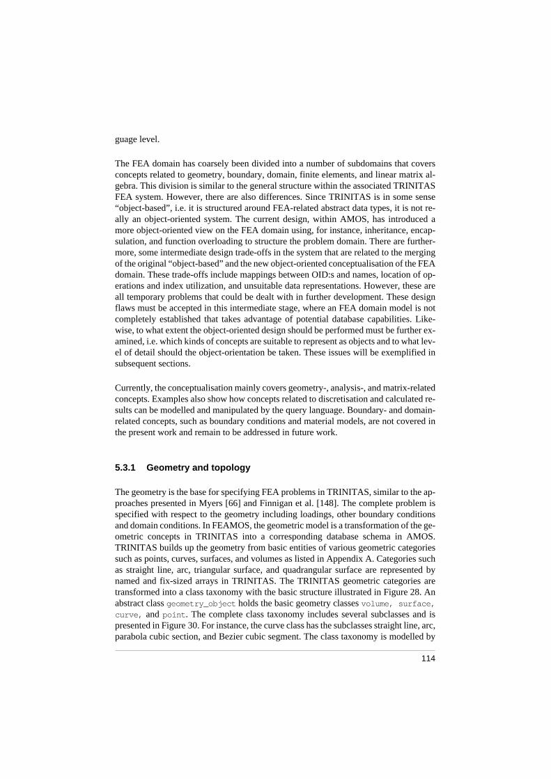
114

guage level.

The FEA domain has coarsely been divided into a number of subdomains that coversconcepts related to geometry, boundary, domain, finite elements, and linear matrix al-gebra. This division is similar to the general structure within the associated TRINITASFEA system. However, there are also differences. Since TRINITAS is in some sense“object-based”, i.e. it is structured around FEA-related abstract data types, it is not re-ally an object-oriented system. The current design, within AMOS, has introduced amore object-oriented view on the FEA domain using, for instance, inheritance, encap-sulation, and function overloading to structure the problem domain. There are further-more, some intermediate design trade-offs in the system that are related to the mergingof the original “object-based” and the new object-oriented conceptualisation of the FEAdomain. These trade-offs include mappings between OID:s and names, location of op-erations and index utilization, and unsuitable data representations. However, these areall temporary problems that could be dealt with in further development. These designflaws must be accepted in this intermediate stage, where an FEA domain model is notcompletely established that takes advantage of potential database capabilities. Like-wise, to what extent the object-oriented design should be performed must be further ex-amined, i.e. which kinds of concepts are suitable to represent as objects and to what lev-el of detail should the object-orientation be taken. These issues will be exemplified insubsequent sections.

Currently, the conceptualisation mainly covers geometry-, analysis-, and matrix-relatedconcepts. Examples also show how concepts related to discretisation and calculated re-sults can be modelled and manipulated by the query language. Boundary- and domain-related concepts, such as boundary conditions and material models, are not covered inthe present work and remain to be addressed in future work.

5.3.1 Geometry and topology

The geometry is the base for specifying FEA problems in TRINITAS, similar to the ap-proaches presented in Myers [66] and Finnigan et al. [148]. The complete problem isspecified with respect to the geometry including loadings, other boundary conditionsand domain conditions. In FEAMOS, the geometric model is a transformation of the ge-ometric concepts in TRINITAS into a corresponding database schema in AMOS.TRINITAS builds up the geometry from basic entities of various geometric categoriessuch as points, curves, surfaces, and volumes as listed in Appendix A. Categories suchas straight line, arc, triangular surface, and quadrangular surface are represented bynamed and fix-sized arrays in TRINITAS. The TRINITAS geometric categories aretransformed into a class taxonomy with the basic structure illustrated in Figure 28. Anabstract class geometry_object holds the basic geometry classes volume, surface,

curve, and point . The complete class taxonomy includes several subclasses and ispresented in Figure 30. For instance, the curve class has the subclasses straight line, arc,parabola cubic section, and Bezier cubic segment. The class taxonomy is modelled by

115

a type and subtype structure in AMOSQL.

Topology relations, i.e. relations among geometric entities such as faces, edges, andvertices , are modelled as functions between basic geometry classes as illustrated inFigure 29. The forks at the end of the relations indicate many-to-many relationships, i.e.for instance that a surface can have many edges and each curve can be an edge to manysurfaces. Since values of normal and multi-valued stored functions in AMOSQL are un-ordered, the topology functions are represented by vectors to accomplish an ordering ofvertices, edges, etc. For example, the function vertex_vector is defined by:

create function vertex_vector(curve c) -> vector as stored;

In addition, a derived vertices function have been defined for accessing each element

more conveniently in ad hoc queries1:

create function vertices(curve c) -> point p as

select element(vertex_vector(c));

The vertices function provides a relation between a curve instance to its definingpoints with the intuitive direction from the curve to the points, but with applicability inboth directions. Spatial coordinate data is defined for the point class where the posi-

tion function stores the x, y, and z coordinates of a point instance. Coordinates can alsobe retrieved by the derived functions x_coordinate, y_coordinate, and z_coordinate.The position function is currently implemented as a tuple of three reals, which causesunnecessary data conversions in manipulating these data. The implementation of theFEAMOS geometry model uses the previously described matrix package in its imple-mentation in AMOS. This has made it possible to use database representations suitablefor numerical processing, and replacing the tuple representation of the coordinates witha matrix representation eliminates the need for data conversions and facilitates numer-ical processing of coordinate data.

In addition, to keep an intermediate correspondence with TRINITAS, a number of at-tributes are currently defined for different geometric categories but might later suit bet-ter in other concept classes. These attributes are located below the dashed lines inFigure 28. There are no absolute truths on how to locate attributes to specific conceptsand this issue will not be discussed in any depth. A good conceptualisation is most cer-tainly based on knowledge about the domain, experience in domain modelling, and aniterative evolution of the design. As an example, the curve type currently has a divi-

sion and a density function implemented. The division function represents thenumber of subdivisions a specific curve is divided into and the density function rep-resents a node density along a curve. Further studies might reveal that it would be moreconvenient to associate these attributes to a mesh concept related to the curve since the

1. It should be noted that an extension of AMOSQL to handle ordered sets, or sequenc-es, can eliminate the need for the vertices function .

116

division and density are, in fact, attributes related to the discretisation of a geometry.However, other issues, such as model complexity and processing efficiency, can influ-ence the outcome of these decisions as well.

Figure 28. Basic type taxonomy for geometry-related concepts in the application domain, where arrows denote is-a (subtype to supertype) relations.

Even if the geometric schema includes those geometric concept classes of TRINITAS,the geometric schema is designed in a general manner to be applicable in other applica-tions as well. There is no application-specific information represented in the basic geo-metric model. Where applicable, relations are established with object identifiers(OID:s) instead of using names and naming conventions. The geometric model can eas-ily be evolved with new geometric concepts or the schema can be changed without af-fecting the application. The application communicates with the general geometry modelthrough a set of derived functions that form a view of the geometry model that can betailored for a specific application. For example, TRINITAS currently uses application-generated names to refer to “objects”. In the geometry model of FEAMOS, these names

Geom. obj.Name

VolumeExists vol.

SurfaceExists sur.

CurveExists curve

PointExists point

Vertices

Exists obj.InitialiseDestruct

Faces Edges

------

Position

Division------N.elementsElement set Element typeN.node elemN.nodesNode setNode deriv.Material

Density

1D VolumeCross section

2D VolumeThickness

3D Volume

X coord.Y coord.Z coord.

Face vector Edge vector Vertex vector

117

are not used for references but they are stored as redundant information in the databaseand used for interfacing between this database and the application.

Figure 29. Topological relations (rectangular symbols) between basic geometry concepts with the intuitive direction indicated by triangular arrowheads.

Operations on geometrical objects are implemented by means of AMOSQL functionsand procedures. TRINITAS operations can be divided into basic operations and com-posite operations. Basic operations include creation and deletion of geometric entitiesas well as operations for accessing and changing their properties. Composite operationsare more complex and usually more domain-oriented operations such as finding specif-ic sets of geometric entities, or calculating geometry-dependent quantities.

Volume

Faces

Surface

Edges

Curve

Vertices

Point

118

Figure 30. The current type taxonomy for the geometric model in FEAMOS.

Since the composite operations partly include basic operations, this initial representa-tion of the geometry model within the database has focused on including the set of basicoperations that can be seen as the actual application interface to the geometry model.When more and more functionality is transferred to the DBMS, this interface will growto incorporate more domain-specific operations. Hence, there are database operations

geometric object

volume

1d volume

constant cross section

triangular section

2d volume

quadrangular sectionpolygon sectiontriangular torusquadrangular toruspolygon torus

3d volume

tetrahedronpentahedronhexahedronextruded polyhedron

surface

triangularquadrangularcylindrical

curve

straight linearcparabola cubic sectionbezier cubic segment

point

polygonic

119

implemented for constructing and destructing geometry objects. For this purpose, itwould be convenient to be able to define tailored constructors and destructors that canbe overloaded. The AMOS system did not permit this kind of definition at the timewhen the geometry model was implemented. However, this was later implemented tobe used for matrices, described in Section 5.2.4. Later again, this functionality has beengeneralised by Werner [93] and implemented in AMOS. Currently, the geometry modelstill uses specialised procedures for creating points, straight lines, etc., but these can lat-er easily be replaced by overloaded constructors. Furthermore, the access functions andthe update procedures have been implemented as derived AMOSQL functions in termsof basic stored functions. In this manner, the application interface forms a view to thedatabase schema supporting a data-independent design.

In FEAMOS, when a geometry is modelled in TRINITAS, an object structure is gener-ated in an AMOS database. The original FORTRAN procedures that handle geometryin TRINITAS have been redesigned to use the AMOS C interface procedures to com-municate with the DBMS. There is no redundant representation of the application mod-el, it exists only within the database. Thus, when an object is manipulated, as for in-stance moving a point in a geometry model on the screen, it implies a direct update ofthe database object.

The modelling of a geometry can be illustrated by means of the example shown inFigure 31. The picture shows a rectangular plate that is fixed on a wall at its left sideand is further exposed to a distributed and uniform pressure load at the upper edge. Inthis case, the geometry model is formed by a number of basic geometric elements, i.e.4 points, 4 straight lines, 1 surface element, and 1 volume element, shown in Figure 32.

This can be expressed in AMOSQL1 as:

create point(name, position) :p1(“p1”, <0.0, 0.0, 0.0>), :p2(“p2”, <0.0, 120.0, 0.0>), :p3(“p3”, <90.0, 120.0, 0.0>), :p4(“p4”, <90.0, 0.0, 0.0>);

create straight_line(name, vertex_vector, division, density) :l1(“l1”, {:p1, :p2}, 3.0, 0.0), :l2(“l2”, {:p2, :p3}, 3.0, 0.0), :l3(“l3”, {:p3, :p4}, 3.0, 0.0), :l4(“l4”, {:p4, :p1}, 3.0, 0.0);

create quadrangular_surface(name, edge_vector) :s1(“s1”,{:l1, :l2, :l3, :l4});

1. To facilitate the interpretation, an interactive style of programming is used the ex-ample in contrast with using the application programming interface for expressingthe same functionality.

120

create quadrangular_section_volume(name, face_vector) :v1(“v1”, {:s1});

These statements create a geometric model where the geometric objects are structuredas illustrated in Figure 33. Through TRINITAS, the model is built up graphically andthe result is illustrated in Figure 34.

Figure 31. A simple physical structure consisting of a fixed plate that is exposed to a distributed and uniform pressure load.

The AMOSQL query language can then be used to formulate queries to the model aboutits structure and content, such as basic geometrical and topological information. For ex-ample the edges of :s1 can be extracted by:

edges(:s1);OID[0x0:765] OID[0x0:766] OID[0x0:767] OID[0x0:764]

Similarly, the edges can be extracted from :v1 by:

edges(faces(:v1));

120

90

121

OID[0x0:765] OID[0x0:766] OID[0x0:767] OID[0x0:764]

Actually, to be sure that an edge will only occur once if it is of several surfaces that form

a volume, the query should be reformulated, using the unique 1 function, as:

unique(edges(faces(:v1)));

If it is common to access the points from other levels than at the curve level, it can beconvenient to overload the vertices function as a derived function on other geometricclasses as well:

create function vertices(volume v) -> point p as

select p for each curve c

where p = unique(vertices(c)) and

c = unique(edges(faces(v)));

Figure 32. Basic geometrical model of the structure in Figure 31 including boundary conditions.

By applying the edges function in the opposite direction, we can find the surface that aspecific curve is a part of:

1. The unique function is an aggregation function that eliminates duplicates from amultiset.

L2

L1

P4 P3

P1 P2

L3

L4 S1, V1

122

select s for each surface s where edges(s) = :l2;

OID[0x0:768]

The edges function is modelled to store object identifiers internally for generality andefficiency reasons. However, the name function can also be applied on each object forname reference. The first of the preceding examples would then look like:

name(edges(:s1));

“L2“ “L3“ “L4“ “L1“

Figure 33. The structure of an instance model of a simple geometric model in FEAMOS.

In addition to basic operations for managing data, the application includes more com-plex and composite operations that form the domain functionality of the application. Asargued at the beginning of this section, there are several factors that influence the deci-sion of where to place operations. Additionally, it might imply a severe redesign of theapplication logic when operations implemented in a conventional and procedural pro-gramming language should be expressed in a database language that is of a more declar-ative nature. Geometric information is involved in many tasks within FEA that arespread all around the application. A redesign at the global level has currently not beenconsidered within FEAMOS, that covers the complete use of geometry information.Nevertheless, a few examples will show how AMOSQL can be used to model morecomplex and composite geometric operations.

v1

s2

l1 l2 l3 l4

p1 p2 p3 p4 p1

Faces

Edges

VerticesVerticesVerticesVertices

123

Operations on geometry to find different sets of boundary objects of the geometry oc-curring frequently. For instance, TRINITAS includes an operation for retrieving thecorners of different geometric entities. In AMOSQL, this is expressed for a quadrangu-lar section in the corners function as:

create function corners(quadrangular_surface qs) -> point as

select p1 for each curve c1, curve c2, point p1

where c1 = edges(qs) and

c2 = edges(qs) and

c1 < c2 and

p1 = vertices(c1) and

p1 = vertices(c2);

Figure 34. The geometry model example modelled in TRINITAS completed with boundary conditions in the form of a fixed boundary and a distributed and uniform load.

Currently, AMOSQL mainly support bag-valued functions. This means that functionsin general return multisets and for obtaining sets the application of additional filtering

124

functions is required. In, for instance, the corners function this has been avoided byreducing the qualifying data sets by replacing the != (not equal to) function by the <

(less than) function. There is a common interest in engineering applications to be ableto handle sets and ordered sets (or sequences), in addition to multisets. AlthoughAMOSQL supports data types for sets and sequences, queries can currently not auto-matically handle and preserve ordering and duplication elimination. A support for han-dling sequences and sets in queries will facilitate the specification of common applica-tion-specific operations where unique and ordered results are desirable. Future incorpo-ration of this functionality in AMOSQL is being considered.

Applying the corner function to our geometry example should return the four cornerpoints of our model as:

select name(corners(s)) for each surface s;“P3“ “P4“ “P2“ “P1“

The compact expressiveness of AMOSQL is illustrated by a comparison with the cor-responding GET_SURFACE_CORNER_POINTS procedure in TRINITAS:

SUBROUTINE GET_SURFACE_CORNER_POINTS(CORNERS,LINES,UNIQUE_POINTS)

INTEGER CORNERS,TYPE,I,J,K,NHITCHARACTER LINES(1)*8,POINTS(4)*8,UNIQUE_POINTS(1)*8,

% END_POINTS(2)*8NHIT = 0DO 10 I=1,CORNERS

CALL GET_LINE(LINES(I),TYPE,POINTS)CALL GET_LINE_END_POINTS(TYPE,POINTS,END_POINTS)DO 20 J=1,2

DO 30 K=1,NHITIF(UNIQUE_POINTS(K).EQ.END_POINTS(J)) GOTO 20

30 CONTINUENHIT = NHIT + 1UNIQUE_POINTS(NHIT) = END_POINTS(J)

20 CONTINUE10 CONTINUE

END

In the TRINITAS procedure the specific surface is implicitly defined by its edges thatare passed as the LINES argument. Here is also an additional argument, CORNERS, thatmust be bound before calling the procedure as exemplified in the GET_SURFACE_CG pro-cedure below.

SUBROUTINE GET_SURFACE_CG(SURFACE_NAME,TYPE,LINES,TP)INTEGER SC(3),TP(2)INTEGER TYPE,I,CORNERS,GET_NO_SURFACE_LINESREAL*4 GC(3),GC0(3)CHARACTER LINES(1)*8,POINTS(20)*8,SURFACE_NAME*8

125

C Get number of surface cornersCORNERS = GET_NO_SURFACE_LINES(SURFACE_NAME,TYPE)

C Get all unique corner pointsCALL GET_SURFACE_CORNER_POINTS(CORNERS,LINES,POINTS)

C Calculate the centre of gravityGC0(1) = 0.GC0(2) = 0.GC0(3) = 0.DO 10 I=1,CORNERS

CALL GET_POINT(POINTS(I),GC)GC0(1) = GC0(1) + GC(1)GC0(2) = GC0(2) + GC(2)GC0(3) = GC0(3) + GC(3)

10 CONTINUEGC0(1) = GC0(1)/CORNERSGC0(2) = GC0(2)/CORNERSGC0(3) = GC0(3)/CORNERSCALL GET_SCREEN_COORDINATE(GC0,SC)TP(1) = SC(1)TP(2) = SC(2)END

Similar observations can be made, as in the previous example, when comparing with

the corresponding functionality expressed in the AMOSQL centroid 1 function:

create function centroid(quadrangular_surface qs) -> <real x,real y,real z> as

select x,y,z where

x = mean(x_coordinate(corners(qs))) and y = mean(y_coordinate(corners(qs))) and z = mean(z_coordinate(corners(qs)));

where mean is an aggregation function that calculates the numerical mean value of itsargument. An application of centroid to our example looks like:

centroid(OID[0x0:768]); <40.,50.,0.>

An additional example shows an AMOSQL function, opposing_curves , for extractingpairs of curves that are opposite for a quadrangular surface.

create function opposing_curves(quadrangular_surface qs) -> <curve c1, curve c2> as

select unique((select c1,c2

1. It should be noted that for a general quadrangular, a more advanced calculation ofthe centroid is required. This functionality is currently absent in TRINITAS.

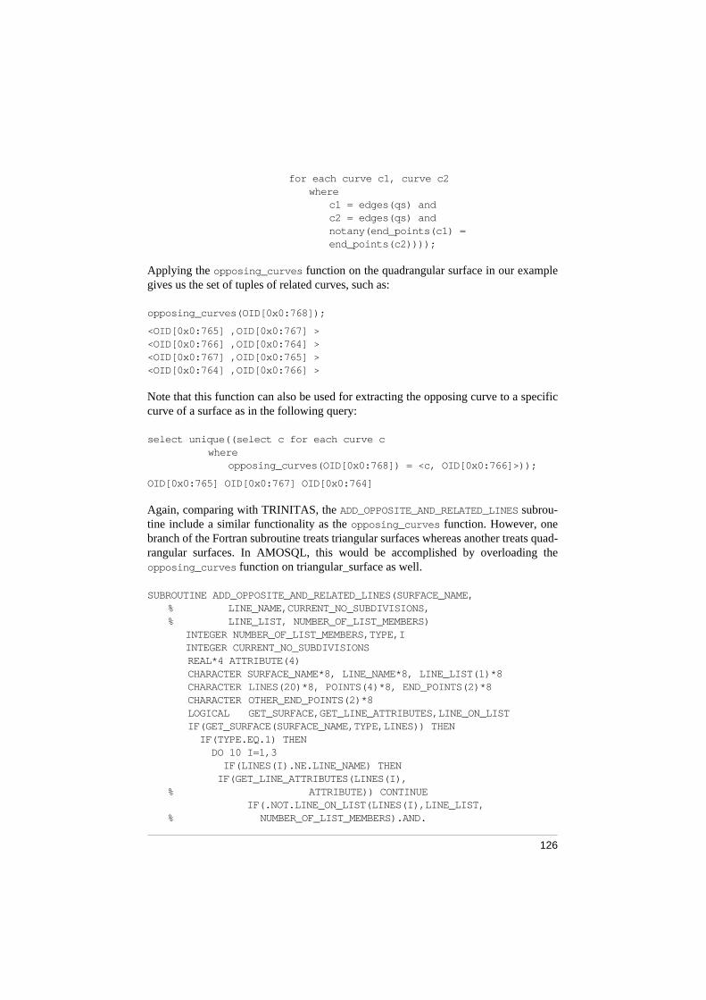
126

for each curve c1, curve c2 where

c1 = edges(qs) and c2 = edges(qs) and notany(end_points(c1) = end_points(c2))));

Applying the opposing_curves function on the quadrangular surface in our examplegives us the set of tuples of related curves, such as:

opposing_curves(OID[0x0:768]);

<OID[0x0:765] ,OID[0x0:767] ><OID[0x0:766] ,OID[0x0:764] ><OID[0x0:767] ,OID[0x0:765] ><OID[0x0:764] ,OID[0x0:766] >

Note that this function can also be used for extracting the opposing curve to a specificcurve of a surface as in the following query:

select unique((select c for each curve c where

opposing_curves(OID[0x0:768]) = <c, OID[0x0:766]>));

OID[0x0:765] OID[0x0:767] OID[0x0:764]

Again, comparing with TRINITAS, the ADD_OPPOSITE_AND_RELATED_LINES subrou-tine include a similar functionality as the opposing_curves function. However, onebranch of the Fortran subroutine treats triangular surfaces whereas another treats quad-rangular surfaces. In AMOSQL, this would be accomplished by overloading theopposing_curves function on triangular_surface as well.

SUBROUTINE ADD_OPPOSITE_AND_RELATED_LINES(SURFACE_NAME,% LINE_NAME,CURRENT_NO_SUBDIVISIONS, % LINE_LIST, NUMBER_OF_LIST_MEMBERS) INTEGER NUMBER_OF_LIST_MEMBERS,TYPE,I INTEGER CURRENT_NO_SUBDIVISIONS

REAL*4 ATTRIBUTE(4)CHARACTER SURFACE_NAME*8, LINE_NAME*8, LINE_LIST(1)*8 CHARACTERLINES(20)*8, POINTS(4)*8, END_POINTS(2)*8 CHARACTEROTHER_END_POINTS(2)*8 LOGICAL GET_SURFACE,GET_LINE_ATTRIBUTES,LINE_ON_LISTIF(GET_SURFACE(SURFACE_NAME,TYPE,LINES)) THEN IF(TYPE.EQ.1) THEN DO 10 I=1,3 IF(LINES(I).NE.LINE_NAME) THEN IF(GET_LINE_ATTRIBUTES(LINES(I),

% ATTRIBUTE)) CONTINUE IF(.NOT.LINE_ON_LIST(LINES(I),LINE_LIST,

% NUMBER_OF_LIST_MEMBERS).AND.

127

% INT(ATTRIBUTE(1)).NE.CURRENT_NO_SUBDIVISIONS) THEN

NUMBER_OF_LIST_MEMBERS = % NUMBER_OF_LIST_MEMBERS + 1

LINE_LIST(NUMBER_OF_LIST_MEMBERS) = LINES(I) END IF END IF

10 CONTINUE ELSE IF(TYPE.EQ.2) THEN CALL GET_LINE(LINE_NAME,TYPE,POINTS) CALL GET_LINE_END_POINTS(TYPE,POINTS,END_POINTS) DO 20 I=1,4 CALL GET_LINE(LINES(I),TYPE,POINTS) CALL GET_LINE_END_POINTS(TYPE,POINTS,

% OTHER_END_POINTS) IF(END_POINTS(1).NE.OTHER_END_POINTS(1).AND.

% END_POINTS(1).NE.OTHER_END_POINTS(2).AND.% END_POINTS(2).NE.OTHER_END_POINTS(1).AND.% END_POINTS(2).NE.OTHER_END_POINTS(2)) THEN

IF(GET_LINE_ATTRIBUTES(LINES(I),% ATTRIBUTE)) CONTINUE

IF(.NOT.LINE_ON_LIST(LINES(I),LINE_LIST,% NUMBER_OF_LIST_MEMBERS).AND.% INT(ATTRIBUTE(1)).NE.CURRENT_NO_SUBDIVISIONS)

THEN NUMBER_OF_LIST_MEMBERS=NUMBER_OF_LIST_MEMBERS+1 LINE_LIST(NUMBER_OF_LIST_MEMBERS) = LINES(I) END IF

END IF20 CONTINUE

END IFEND IFEND

The preceding examples of operations on the geometry mainly considered the retrievalof topologic information, but also included some calculation of geometric information,in terms of the centre of gravity, in the centroid function. Another geometric operation,is to find the nearest point to a given point (or position), by calculating the minimal dis-tance. In TRINITAS, this is accomplished by the FIND_NEAREST_POINT procedure. Thedistance calculation is carried out in the GET_SCREEN_DISTANCE procedure.

LOGICAL FUNCTION FIND_NEAREST_POINT(C,PICKED_POINTS,% NO_PICKED_POINTS,% NEAREST_POINT_NAME, % SCREEN_COORDINATE)

INTEGER SCREEN_COORDINATE(3),C(1),SC(3)INTEGER NPOINTS,I,NO_PICKED_POINTS,JREAL*4 DISTANCE,GET_SCREEN_DISTANCE,MIN_DISTANCE,GC(3)LOGICAL GET_POINT

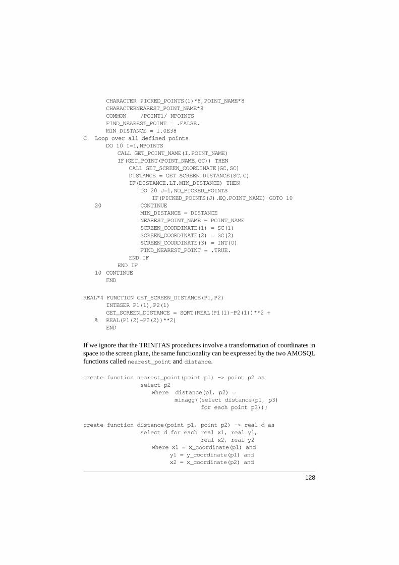
128

CHARACTERPICKED_POINTS(1)*8,POINT_NAME*8CHARACTERNEAREST_POINT_NAME*8COMMON /POINT1/ NPOINTSFIND_NEAREST_POINT = .FALSE.MIN_DISTANCE = 1.0E38

C Loop over all defined pointsDO 10 I=1,NPOINTS

CALL GET_POINT_NAME(I,POINT_NAME)IF(GET_POINT(POINT_NAME,GC)) THEN

CALL GET_SCREEN_COORDINATE(GC,SC)DISTANCE = GET_SCREEN_DISTANCE(SC,C)IF(DISTANCE.LT.MIN_DISTANCE) THEN

DO 20 J=1,NO_PICKED_POINTSIF(PICKED_POINTS(J).EQ.POINT_NAME) GOTO 10

20 CONTINUEMIN_DISTANCE = DISTANCENEAREST_POINT_NAME = POINT_NAMESCREEN_COORDINATE(1) = SC(1)SCREEN_COORDINATE(2) = SC(2)SCREEN_COORDINATE(3) = INT(0)FIND_NEAREST_POINT = .TRUE.

END IFEND IF

10 CONTINUEEND

REAL*4 FUNCTION GET_SCREEN_DISTANCE(P1,P2)INTEGER P1(1),P2(1)GET_SCREEN_DISTANCE = SQRT(REAL(P1(1)-P2(1))**2 +

% REAL(P1(2)-P2(2))**2)END

If we ignore that the TRINITAS procedures involve a transformation of coordinates inspace to the screen plane, the same functionality can be expressed by the two AMOSQLfunctions called nearest_point and distance .

create function nearest_point(point p1) -> point p2 asselect p2

where distance(p1, p2) = minagg((select distance(p1, p3)

for each point p3));

create function distance(point p1, point p2) -> real d as select d for each real x1, real y1,

real x2, real y2 where x1 = x_coordinate(p1) and

y1 = y_coordinate(p1) and x2 = x_coordinate(p2) and

129

y2 = y_coordinate(p2) and d = sqrt((x2*x2-x1*x1) + (y2*y2-y1*y1));

The application of the nearest_point and the distance functions, by means of an ad-ditional test point :pa, in our example looks like:

create point(name, position) :pa(“pa”, <100.0, 100.0, 0.0>);

name(nearest_point(:pa));<“P3”>

distance(:pa, :p3);

<42.4264>

select name(p),distance for each point p, real distance where nearest_point(:pa) = p and

distance = distance(:pa, p);

<“P3”,42.4264>

It should be noted that in the general three-dimensional case the distance and thenearest_point function can be overloaded on lines instead of points. A screen posi-tion can then be viewed as a straight line perpendicular to the screen which makes itpossible to calculate and compare the distances in terms of the actual point coordinatesof the geometry model. This opens the possibility of using spatial indexing techniquesto make the search in the point space more efficient. As the set of points in the pointspace becomes large, spatial indexing techniques can dramatically reduce search effort.However, this issue must be studied in more detail before any specific conclusions canbe drawn. There are other FEA data sets as well where spatial indexing can be advan-tageous. This includes the discretisation of the geometry into mesh data and calculationof quantities, such as stress and displacement fields, distributed over the geometry.Hence, the potential benefit of spatial indexing for different FEA tasks must be evalu-ated to avoid sub-optimizations.

Several spatial indexing techniques are based on a tree representation where the accesscost is dependent on the depth of the tree. An approximated measure of the access cost,Ca, can be expressed in terms of the indexed data set N; we get . This cost

should be compared to the current access cost using linear search (i.e. no indexes) isproportional to N.

There is currently no spatial indexing technique available in AMOS and a future re-search area would be to investigate how spatial indexes could make spatially-relatedqueries more efficient. To be able to make relevant conclusions, this work should prob-ably include comparisons on how indexing, filtering, as well as the location of data andprocessing influence the total processing costs for different operations, as pointed outin Section 5.1.

Ca Nlog∼

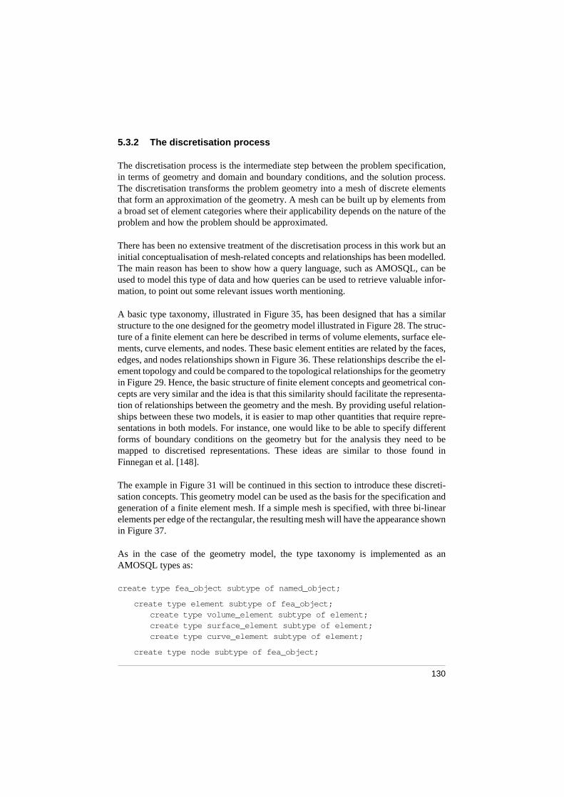
130

5.3.2 The discretisation process

The discretisation process is the intermediate step between the problem specification,in terms of geometry and domain and boundary conditions, and the solution process.The discretisation transforms the problem geometry into a mesh of discrete elementsthat form an approximation of the geometry. A mesh can be built up by elements froma broad set of element categories where their applicability depends on the nature of theproblem and how the problem should be approximated.

There has been no extensive treatment of the discretisation process in this work but aninitial conceptualisation of mesh-related concepts and relationships has been modelled.The main reason has been to show how a query language, such as AMOSQL, can beused to model this type of data and how queries can be used to retrieve valuable infor-mation, to point out some relevant issues worth mentioning.

A basic type taxonomy, illustrated in Figure 35, has been designed that has a similarstructure to the one designed for the geometry model illustrated in Figure 28. The struc-ture of a finite element can here be described in terms of volume elements, surface ele-ments, curve elements, and nodes. These basic element entities are related by the faces,edges, and nodes relationships shown in Figure 36. These relationships describe the el-ement topology and could be compared to the topological relationships for the geometryin Figure 29. Hence, the basic structure of finite element concepts and geometrical con-cepts are very similar and the idea is that this similarity should facilitate the representa-tion of relationships between the geometry and the mesh. By providing useful relation-ships between these two models, it is easier to map other quantities that require repre-sentations in both models. For instance, one would like to be able to specify differentforms of boundary conditions on the geometry but for the analysis they need to bemapped to discretised representations. These ideas are similar to those found inFinnegan et al. [148].

The example in Figure 31 will be continued in this section to introduce these discreti-sation concepts. This geometry model can be used as the basis for the specification andgeneration of a finite element mesh. If a simple mesh is specified, with three bi-linearelements per edge of the rectangular, the resulting mesh will have the appearance shownin Figure 37.

As in the case of the geometry model, the type taxonomy is implemented as anAMOSQL types as:

create type fea_object subtype of named_object;

create type element subtype of fea_object;create type volume_element subtype of element;create type surface_element subtype of element;create type curve_element subtype of element;

create type node subtype of fea_object;

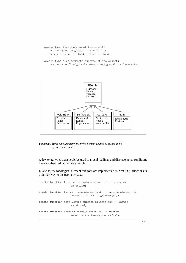
131

create type load subtype of fea_object;create type line_load subtype of load;create type point_load subtype of load;

create type displacements subtype of fea_object;create type fixed_displacements subtype of displacements;

Figure 35. Basic type taxonomy for finite element-related concepts in the application domain.

A few extra types that should be used to model loadings and displacements conditionshave also been added in this example.

Likewise, the topological element relations are implemented as AMOSQL functions ina similar way to the geometry case.

create function face_vector(volume_element ve) -> vector as stored;

create function faces(volume_element ve) -> surface_element asselect element(face_vector(ve));

create function edge_vector(surface_element se) -> vector as stored;

create function edges(surface_element se) -> vector select element(edge_vector(se));

FEA obj.Exist obj.

Volume el.Exists v. el.

Surface el.Exists s. el.

Curve el.Exists c. el.

NodeExists node

Nodes

InitialiseDestruct

Faces Edges Position

Name

Face vector Edge vector Node vector

132

create function edge(surface_element se) -> curve_element asselect element(edge_vector(se));

create function node_vector(element e) -> vector as stored;

create function nodes(element e) -> node as select element(node_vector(e));

Figure 36. Topological relationships between basic FEA element concepts.

It is then possible to populate a database with element and node objects. This is done bycontinuing to populate our geometrical database. Thus, the element structure inFigure 37 can be created by the following AMOSQL statements:

create node (name) :n1 (“n1”), :n2 (“n2”), ... :n16 (“n16”);

create curve_element (name, node_vector) :ce1 (“ce1”, {:n1,:n2}), :ce2 (“ce2”, {:n2,:n3}), ... :ce24 (“ce24”, {:n15,:n16});

Volume el.

Faces

Surface el.

Edges

Curve el.

Nodes

Node

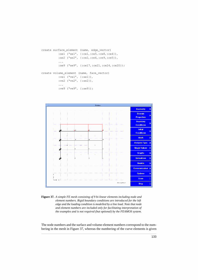
133

create surface_element (name, edge_vector) :se1 (“se1”, {:ce1,:ce5,:ce8,:ce4}), :se2 (“se2”, {:ce2,:ce6,:ce9,:ce5}), ... :se9 (“se9”, {:ce17,:ce21,:ce24,:ce20});

create volume_element (name, face_vector) :ve1 (“ve1”, {:se1}), :ve2 (“ve2”, {:se2}), ... :ve9 (“ve9”, {:se9});

Figure 37. A simple FE mesh consisting of 9 bi-linear elements including node and element numbers. Rigid boundary conditions are introduced for the left edge and the loading condition is modelled by a line load. Note that node and element numbers are included only for facilitating interpretation of the examples and is not required (but optional) by the FEAMOS system.

The node numbers and the surface and volume element numbers correspond to the num-bering in the mesh in Figure 37, whereas the numbering of the curve elements is given

134

in Figure 38. To facilitate the interpretation of the element and node structure an in-stance model for one of the nine elements is given Figure 39. There are actually ninesimilar instance models that share elements and nodes on several levels.

Figure 38. The labels assigned to the curve elements in the mesh example illustrated in Figure 37.

It is now possible to state queries to this database model of the mesh. For instance, thenodes of a curve element can be retrieved:

name(nodes(:ce2));

“n2” “n3”

Another example retrieves the edges of a surface element:

name(edges(:se2));

“ce2” “ce6” “ce9” “ce5”

These basic functions can further be overloaded, as derived functions, on additionaltypes to get a convenient retrieval capability. For instance, the nodes and the edges

functions are here overloaded on additional element types.

create function nodes(surface_element se) -> node n as

select unique(nodes(edges(se)));

create function nodes(volume_element ve) -> node n as

select unique(nodes(edges(faces(ve))));

CE1 CE2 CE3

CE4 CE5 CE6 CE7

CE8 CE9 CE10

CE11 CE12 CE13 CE14

CE15 CE16 CE17

CE18 CE19 CE20 CE21

CE22 CE23 CE24

135

create function edges(volume_element ve) -> curve_element ce as select edges(faces(ve));

With this capability, we can easily retrieve nodes for surface elements and nodes andedges for volume elements.

name(nodes(:se2));“n2” “n3” “n7” “n6”

name(nodes(:ve1));“n1” “n2” “n6” “n5”

name(edges(:ve1));“ce1” “ce5” “ce8” “ce4”

Figure 39. The structure of an instance model for one of the volume elements in the mesh example.

Furthermore, the same functions can be applied in the reverse direction to find out inwhich elements a specific node appears.

select name(ve) for each volume_element ve where nodes(ve) = :n1;“ve1”

select name(ve) for each volume_element ve where nodes(ve) = :n10;“ve4” “ve5” “ve7” “ve8”

ve1

se2

ce1 ce5 ce8 ce4

n1 n2 n6 n5 n1

Faces

Edges

NodesNodesNodesNodes

136

So far, this description has only concerned the mesh structure itself, but it is now timeshow how it can be connected to the geometry. A good idea is to separate the discreti-sation and the geometry as much as possible, which has already accomplished. Further,the discretisation is probably more dependent on the geometry than the opposite. By de-fining functions between mesh and geometry on the mesh concepts, the geometry con-ceptualisation becomes independent of the discretisation conceptualisation. Hence,mesh concepts are tied to the corresponding geometric concepts by the following func-tions.

create function volume(volume_element ve) -> volume as stored;create function surface(surface_element se) -> surface as stored;create function curve(curve_element ce) -> curve as stored;create function point(node n) -> point as stored;

These functions must further be populated by appropriate values.

set volume(:ve1) = :v1;set volume(:ve2) = :v1;...set volume(:ve9) = :v1;

set surface(:se1) = :s1;set surface(:se2) = :s1;...set surface(:se9) = :s1;

set curve(:ce1) = :c1;set curve(:ce2) = :c1;...set curve(:ce18) = :c4;

set point(:n1) = :p1;set point(:n4) = :p2;set point(:n16) = :p3;set point(:n13) = :p4;

Now, relationships across are established and information can be retrieved about theserelationships. For instance, it is possible to retrieve the position of the points that definethe curve that the curve element :ce11 is associated to.

select position(p) for each point p, curve c where curve(:ce11) = c and vertices(c) = p;<10.,70.,0.><10.,30.,0.>

Maybe it would be more interesting to be able to extract information about loading anddisplacement conditions. To show how this can be accomplished a few properties aredefined for line loads and fixed displacements. To be able to define where the load or

137

the fixation should act, a curve function is defined for each concept. For the line loadan additional intensity function is defined to represent the load intensity.

create function curve(line_load l) -> curve as stored;create function intensity(line_load l) -> real as stored;create function curve(fixed_displacements d) -> curve as stored;

Then, a specific load and fixation is created:

create line_load(name, curve, intensity) :ll1(“ll1”, :c3, -1000.0);

create fixed_displacements(name, curve) instances :fd1(“fd1”, :c4);

When the discretised model should be established in an FEA, one would like to knowwhich nodes boundary conditions are acting on. These nodes can be retrieved in ourmodel. For example, the nodes that are influenced by the line load can be retrieved bythe following query:

select distinct 1 name(n) for each node n, curve c,curve_element ce, line_load l

where curve(l) = c and curve(ce) = c and nodes(ce) = n;

“n13” “n14” “n15” “n16”

Similarly, the nodes that are influenced by the fixed line is found through the query:

select distinct name(n) for each node n, curve c,curve_element ce, fixed_displacements fd

where curve(fd) = c and curve(ce) = c and nodes(ce) = n;“n1” “n5” “n9” “n13”

Furthermore, if would be possible to eliminate the node that takes part in both the loadand the fixation:

select distinct name(n) for each node n, curve c,curve_element ce, line_load l

where curve(l) = c and curve(ce) = c and nodes(ce) = n and notany(fixed(n));

“n14” “n15” “n16”

1. The distinct keyword tells the select statement to eliminate duplicates in a simi-lar way to the unique operator.

138

In the preceding query a function, fixed , is used that checks if a specific node is fixedand has the following implementation:

create function fixed(node n) -> node as select n where n = (select distinct m for each node m,

curve c, curve_element ce, fixed_displacements fd

where curve(fd) = c and curve(ce) = c and nodes(ce) = m);

Hence, it has been shown how the query language can be used for extracting informa-tion about the mesh and its relationships to geometry and boundary conditions. Severalof these query examples are much more complicated to express in an ordinary program-ming language. However, the conceptualisation must be further developed to incorpo-rate and handle the different element types provided in TRINITAS as outlined inFigure 40.

Figure 40. Outline of a type taxonomy for finite element mesh concepts.

fea object

element

volume element

surface element

curve element

node

3D element

2D element

1D element

element type

bi-linear quadrangle

linear bar

quadratic lagrangequadratic serendipity

constant strain trianglelinear strain triangle

tri-linear hexahedral

non-linear bar

139

Furthermore, it must be evaluated whether the data representations currently providedin AMOS are efficient enough to support discretisation operations. If more efficientdata representations are required, a similar approach to the matrix data source, de-scribed in Section 5.2.3, might be applicable where foreign and specialised data repre-sentations were implemented and made available from AMOS. For this purpose, itmight be suitable to apply a tree data structure as described in Fenves [39].

Finally, it would be most interesting to investigate if function materialisation techniques[149] could be applied in this context to automatically handle computation and cachingof, for instance, derived topology functions.

5.3.3 Finite element analysis solution algorithms

The ability of the DBMS to solve linear equation systems in the FEA process was oneprimary intention of the design and implementation of the linear algebraic matrix alge-bra package that were described in Section 5.2.

For this reason, the type system of AMOS was extended with a set of matrix typesequipped with a basic set of matrix operations that were transparently made availablein the query language. This ability permitted application-specific domain concepts to begiven a suitable representation that were transparently handled through the query lan-guage. Hence, effective data representations could be provided by the DBMS that elim-inate or minimise low-level data administration such as physically copying and trans-forming data.

The solution algorithms of finite element analysis include procedures for numericallysolving linear equation systems. In the FEAMOS system, these algorithms can be ex-pressed in a very natural and high-level terminology by the built-in package for linearmatrix algebra. Application-specific domain concepts that are to be represented by ma-trices are modelled as subtypes of appropriate matrix types. This makes it possible toexpress the corresponding domain operations in terms of these domain-specific matrixconcepts.

We exemplify this by the solution of the previously stated, Eq. (30), linear equation sys-tem K a = f, where K is the stiffness matrix, a is the displacement vector, and f is theload vector. Using domain-specific types, this solution process can be stated in the fol-lowing manner. According to Figure 41, the stiffness matrix, K, is modelled as a sub-type of the symmetric_matrix type; the displacement vector, a, and the load vector, f,are modelled as subtypes of the column_matrix type. Further, by providing a specificdomain type taxonomy for these domain concepts, domain-specific properties can berepresented independently of the mathematical matrix concepts.

However, the corresponding domain operations must be able to generate the correct re-sult type in order to maintain consistency. In the present case, the solution of the linear

140

equation system is performed by applying the operations that correspond to Eqs. (67),in Section 5.2.3. We see that:

(69)

the factorisation of K should return a diagonal matrix and at least one upper unit trian-gular matrix. If we, for instance, consult Hughes [23], we see that the LDL factorisationproduces a diagonal matrix, D, where the matrix elements have the same unit as the el-

ements of K. Further, for the upper and lower unit triangular matrices, U and UT, theelements are unitless. Continuing with the solution of the upper triangular equation sys-tem,

(70)

this operation should produce a displacement vector a. When considering the bbf bind-ing pattern, this operation should produce a displacement vector x, since U is unitless.Consistently, the next diagonal scaling operation

(71)

should generate a displacement vector x with the bfb binding pattern, whereas the bbfbinding pattern should return a load vector y, due to the multiplication of stiffness ele-ments in D with displacement elements in x. Finally, for the operation that solves thelower triangular system

(72)

a load vector y should be produced since f is a load vector and U is unitless. Conse-quently, the bbf binding pattern for this operation returns a load vector with the presentarguments.

If the original matrix multiplication operations have been carefully designed, they willproduce the correct result type for several cases. For instance, in Eqs. (70) and (72), thecorrect type will be produced since it is deduced from one of the argument or resulttypes. However, when the result type is dependent on combinations of argument and re-sult types, as in Eq. (71), special treatment is needed. In the present case, this functionis overloaded for the domain types signatures. Likewise, the result type of D in the fac-torisation operation, corresponding to Eq. (69), is domain-dependent. Here, this is ac-complished by overloading this operation on K.

By using these basic matrix operations, the solution of the system can be stated inAMOSQL in a very convenient notation. Presuming that a stiffness matrix and a loadvector exist and are bound to the interface variables :k and :f respectively, the

Kb

UT( )

fD

fU

f⋅ ⋅=

Ub

af⋅ x

b=

Db

xf⋅ y

b=

UT( )

by

f⋅ fb

=

141

AMOSQL query for solving the displacements would look like:

select a for each displacement_vector a where :k * a = :f;

Figure 41. The representation of application domain types, such as stiffness, loads, and displacements, as subtypes of matrices in the matrix taxonomy. The taxonomy is here somewhat reduced to simplify the presentation.

The stiffness matrix, K, could have been modelled with either of the available represen-tations, i.e. as a subtype of the regular or skyline matrix schemes that implies a reg-ular or a skyline representation of the equation system. However, this does not changethe expression for the solution algorithm and the system automatically creates matriceswith the appropriate types and selects the correct operations to solve the equation sys-tem. By providing several matrix representations schemes, the application can explicit-

matrix

row vector

column vector

square

upper triangular

upper unit triangular

lower triangular

lower unit triangularmatrix scheme

regular

skyline

sparse

symmetric stiffness regular matrix

fea concepts

stiffness

load

displacement

symmetric

diagonal

triangular

diagonal stiffness matrix

load vector

displacement vector

symmetric stiffness skyline matrix

142

ly choose a suitable representation depending on the problem type, or implicitly, by let-ting the query processor make the decision based on type information or a potential costmodel. The DBMS could also support the derivation of the correct type representationby using a derived type mechanism as described in Werner [93], but this facility wasnot available at the time of this work. Thus, the potential convenience of using derivedtypes must be further evaluated.

If the solution algorithm were embedded within an application, it would be suitable torepresent it as a database function that could be accessed from the application. This isexpressed as follows:

create function lin_solve(symmetric_stiffness_regular_matrix k,load_vector f) -> displacement_vector a as

select a where k * a = f;

and overloaded for the skyline representation:

create function lin_solve(symmetric_stiffness_skyline_matrix k,load_vector f) -> displacement_vector a as

select a where k * a = f;

A small example1 in Figure 42 is used to show how this can be used in problem solving.

The compact representation using skyline matrices is assumed in this example. The cre-ation of the basic matrices and the solution of the corresponding equation system areperformed by the following AMOSQL statements:

set :k = construct(“symmetric_stiffness_skyline_matrix”,{{1.0}, {-1.0,2.0},{-1.0,2.0},{-1.0,2.0}}});

set :i = construct(‘iarray’,{0,2,4,6}); 2

set dindex(:k) = :i;

set :f1 = construct(“load_vector”,{1.0,0.0,0.0,0.0});

set :a = solve(:k,:f1);

print(:a);{4,3,2,1}

1. Normally, matrices are created and updated by calling database functions from theapplication which are inconvenient to use in textual examples. The syntax for inter-active manipulation of matrices is somewhat temporary and has been slightly mod-ified to shorten the presentation of the examples.

2. It is not necessary to create the index array :i of the skyline matrix :k explicitly butthis is the current procedure.

143

It is further possible to express the repetitive solution of the same problem for different

load cases by overloading the solve function on bags1 of load vectors. This would beexpressed as:

create function lin_solve(symmetric_stiffness_skyline_matrix k, bag of load_vector f) ->displacement_vector a as

select a where k * a = element(f);

Figure 42. An example equation system with a 4x4 stiffness matrix, a displacement vector with 4 unknowns, and two load vectors including one non-zero component each.

Combining the load_vector :f1 with another called :f2 into a bag :fseq makes it pos-sible to express the corresponding solution in the following manner:

set :f1 = construct(“load_vector”,{1.0,0.0,0.0,0.0});

set :fseq = {:f1,:f2};

set :aseq = lin_solve(:k,:fseq);

print(:aseq,0);{4,3,2,1}

print(:aseq,1);{8,6,4,2}

It should be noted that, by overloading matrix operations, the domain conceptualisationwill hold independently of how each concept is represented or how the operations areimplemented. As discussed earlier, the declarativeness of the query language makes itpossible to achieve both logical and physical data independence. Since the schema in

1. Actually, one would like to have a sequence of load_vector instead of a bag(or multiset) to preserve order but, as have been pointed out earlier, this capabilityis not currently available in AMOSQL.

1 1– 0 0

1– 2 1– 0

0 1– 2 1–

0 0 1– 2

a1

a2

a3

a4

⋅

1

0

0

0

2

0

0

0

,=

144

our case not only includes data descriptions, but also operator descriptions, this inde-pendence of physical and logical implementation becomes valid for operations too.

For instance, in the present context the solution of a triangular equation system A b = c,where A is a triangular matrix and b and c are column vectors, is expressed inAMOSQL as:

select b for each column_vector b where :A * b= :c;

This expression is independent of how the C-procedure that solves this system is imple-mented which results in physical implementation independency.

Furthermore, by replacing the name of the variables in this expression, the expressionsolves a linear equation system K a = f, where K is a symmetric matrix and a and f arecolumn vectors. However, this solution includes a transformation of the equation sys-tem into a set of simpler equations, according to Eq. (68), that is expressed by anAMOSQL expression. The transformation in Eq. (68) could be replaced by a differenttransformation that also solves the linear equation systems, for example by applying adifferent matrix decomposition method. This does not influence the expression of thesolution in terms of the times operator on the highest level. Hence, a form of logical im-plementation independency is achieved.

In this sense, the term “data independence” might be unsuitable to use in some situa-tions and a more suitable term could, for instance, be physical and logical implementa-tion independence.

Since both structure and process of the application domain can be captured, we canmodel complete parts of the domain knowledge independently of any application.Hence, this provides sharing of domain knowledge among applications and further fa-cilitates its reuse. Furthermore, the ability of the query optimizer to handle domainmodels including concepts, data representations, operators, and cost models that are do-main-dependent, can be viewed as a form of domain compilation. Hence, we have a do-main compiler that uses domain knowledge in the compilation process.

Further work in this area would be to develop corresponding domain models for otherparts of the FEA process, such as calculating element quantities including the elementstiffness in Eq. (32) and the element loads in Eq. (33). The possibility of using matrixalgebraic expressions for this purpose must be studied in more detail.

5.3.4 Result evaluation

The result evaluation activity includes calculation and interpretation of various physicalquantities, such as stresses, displacements, and eigenvalues that is evaluated accordingto some design criteria. As illustrated in Figure 43, TRINITAS supports this evaluationgraphically by facilities for displaying, for instance, stress and displacement fields, sin-

145

gle values, multiple values in graphs. The calculated results are stored in arrays that areaccessed by a set of built-in FORTRAN subroutines. By making various menu-basedselections, the user can activate appropriate routines and display the result.

When the basic array-based data storage of TRINITAS was replaced by a correspond-ing array representation in AMOS, it immediately made all data accessible at the arraylevel from the query language. Without any further conceptual modelling, it was possi-ble to state queries over all data, including calculated analysis results.

Since all data are available at the query language level, the user has numerous capabil-ities to compose queries for retrieving, combining, and transforming data. For instance,queries can be stated for retrieving:

• max and min displacements,

• max and min stresses,

• various weighted quantities such as von Mises stresses, etc., and

• quantities combined with additional constraints.

Figure 43. An example that shows how analysis results can be presented to the user in TRINITAS. The picture includes coloured iso-levels of von Mises stresses, the displacement field, and two single stress values.

146

The following query selects a single value from an array1 of von Mises stresses, wherethe index corresponds to a certain node:

ref(array_named(“VON1 “),0);844.779

If one would like to extract the maximum von Mises stress this query can be extendedto traverse the complete array and then apply the max aggregation operator:

select max((select vonmises for each integer i, integer j, real vonmises

where i = iota(0,j) and j = size(array_named(“VON1 “)) - 1and vonmises = ref(array_named(“VON1 “),i)));

2269.62

Further, it is not necessary to store every type of result in the database. Instead, derivedfunctions can be defined that calculate these measures. The ability to do calculationswithin queries is exemplified in the following ad-hoc query where the previous queryis reformulated in terms of the basic stress components:

select max((select vonmises for each integer i, integer j,

real sigmaxx, real sigmayy, real sigmaxy, real vonmises where j = size(array_named(“VON1 “)) - 1 and

i = iota(0,j) and sigmaxx = ref(array_named(“SXX1 “),i) and sigmayy = ref(array_named(“SYY1 “),i) and sigmaxy = ref(array_named(“SXY1 “),i) and vonmises = sqrt(abs(sigmaxx*sigmaxx +

sigmayy*sigmayy - sigmaxx*sigmayy + 3*sigmaxy*sigmaxy))));

2269.62

Associated information can be retrieved by selecting several results in the same query,as in the subsequent query where the stress value is combined with a number corre-sponding to the node number:

select max((select vonmises,i+1for each integer i, integer j, real vonmises

where i = iota(0,j) and j = size(array_named(“VON1 “)) - 1 and vonmises = ref(array_named(“VON1 “),i)));

<2269.62,83>

1. The array_named function maps a name of an array to an array object.

147

The query results can further be filtered by adding additional constraints in the query.Here, the von Mises stresses that exceed 2000.0 (MPa) are extracted along with thenode numbers.

select vonmises,i+1for each integer i, integer j, real vonmises

where i = iota(0,j) and j = size(array_named(“VON1 “)) - 1 andvonmises = ref(array_named(“VON1 “),i) and vonmises > 2000.0;

<2269.62,83><2128.4,90>

The previous examples showed how the current array representation was directly acces-sible from the query language. In comparison to the original TRINITAS program, theexpressibility for accessing and composing data have increased dramatically in FEA-MOS, even if the queries became a bit clumsy on occasion. In addition, it is not so crit-ical if some relevant evaluation functionality has been overlooked in the implementa-tion. It will be relatively simple to add this through the query language. In TRINITAS,this must be done by implementing some new FORTRAN routines.

As was pointed out, the previous examples implied a rather clumsy and unattractive useof the query language. To get rid of this disadvantage, one could introduce much morestructure within the result information through OO modelling. For instance, by associ-ating the stress components to the nodes, the former queries can be expressed and inter-preted much more conveniently. This can be accomplished as:

create function stresses(node n) -> farray as stored;

As we only consider stress components in the xy-plane, the stresses function storesan array of three reals that can represent the stress components σxx, σxy, and σyy. Thesecan be explicitly referenced and defined by derived functions.

create function sigma-xx(node n) -> real as select ref(stresses,0);

create function sigma-xy(node n) -> real as select ref(stresses,1);

create function sigma-yy(node n) -> real as select ref(stresses,3);

create function vonmises(node n) -> real vm as select sqrt(abs(sigma-xx(n)*sigma-xx(n) +

sigma-yy(n)*sigma-yy(n) - sigma-xx(n)*sigma-yy(n) + 3*sigma-xy(n)*sigma-xy(n)));

148

By structuring the stresses along these lines, the previous query for retrieving the max-imum von Mises stress can now be expressed as:

select max((select vonmises(n) for each node n));

Likewise, the node1 can be retrieved together with the von Mises stress:

select max((select vonmises(n),n for each node n));

Additional constraints can easily be introduced in a similar way to the former example,but here the there is a more direct association to the stress function.

select vm for each node n, real vm where vm = vonmises(n) and vm > 2000.0;

It will also be easy to express queries including additional constraints as in the follow-ing query where von Mises stresses within a certain area are extracted:

select n for each node n where vonmises(n) > 0.0 andx_coordinate(n) > 50.0 and x_coordinate(n) < 70.0 and x_coordinate(n) > 40.0 and y_coordinate(n) < 60.0;

Here, it is presupposed that coordinate functions are defined for nodes.

By overloading stress functions on other types, in addition to nodes, it is possible to se-lect stresses along boundary, curves, or other geometrical sections.

Currently, we have the possibility to directly interact with the FEAMOS databasethrough the query language through a database client, shown in Figure 44. This www-based database client uses a general www-interface implemented in AMOS. Within thiswork we have also discussed and planned to implement functions for displaying the re-sult of a query graphically on the analysis model. This type of display function should,for instance, be able to display a set of nodes that have been filtered out as a result of aquery.

Within this context there are also two database mechanisms that ought to be studied infurther research. As indicated in other areas of FEA, indexes can be of great importancefor supporting efficient processing. FEA results, such as stress and temperature fields,are examples of spatial quantities where spatial indexing techniques could be applied.Furthermore, in studying the issue of whether a stored or a derived representation ofanalysis results is preferable, it should be of interest to evaluate how function material-isation techniques [149] could support these decisions in an automatic manner.

1. Note that the node is here an object and not a number as in the previous example.

149

Figure 44. An illustration of the use of a www-based database client in combination with FEAMOS for providing ad-hoc query capabilities.

Even if the user can get great support from graphics and a query language, as describedhere, the result interpretation is mainly a manual activity. The efficiency and qualitycould probably be increased for this activity by taking advantage of the rule system inAMOS. By defining active rules that interpret the results, parts of the evaluation activitycould probably be automated. The applicability of these ideas requires additional study.

5.4 PERFORMANCE ISSUES

As pointed out earlier in this thesis, performance is of vital importance for FEA appli-cations since large data volumes, and complex and costly operations are involved. It is,moreover, important to attain good performance on the average as well as good scale-up characteristics. Furthermore, for interactive FEA applications it is important that theresponse time is acceptable for the activities that are to be performed.

150

Since this work does not cover a final and complete implementation of an FEA appli-cation, it is not possible to make a complete performance evaluation either. However,the FEAMOS system is complete in the sense that it is possible to perform completeanalyses to demonstrate its current capabilities. This makes it possible compare the per-formance of subactivities in the analysis process where alternative implementationtechniques exist for FEAMOS with respect to TRINITAS.

One of the first performance evaluations made in this work, [7], was to compare the ef-ficiency of FEAMOS and TRINITAS of creating and accessing simple data entities. Amajor reason was to evaluate the interface overhead for accessing the database in FEA-MOS compared to accessing a Fortran array in TRINITAS. The performance test meas-ured the time for the creation of objects including an initialisation (update) of two storedfunctions. This corresponds to point objects, a name attribute, and a position attributewith three coordinates. We also measured the access time for random access of the samenumber of objects including the access of the name and the position function. These re-sults are presented in Figure 45 and Figure 46. The original figures in Orsborn [7], weremeasured with WS-IRiS, [118], and these have later been updated to be valid forAMOS.

Figure 45. A performance comparison between FEAMOS and TRINITAS. The diagram shows the real time for creating point objects and for accessing the position of randomly chosen point objects. The x-axis represents the number of objects and the y-axis the real execution time in seconds.

0

20

40

60

80

100

120

140

0 2000 4000 6000 8000 10000

FEAMOS create

FEAMOS access

TRINITAS create

TRINITAS access

151

It is seen from the diagrams that TRINITAS has quadratic performance curves whilethe FEAMOS curves show a linear behaviour. The improved behaviour is explained bythe lack of dedicated storage structures in TRINITAS and results in a significantly im-proved performance of FEAMOS in comparison to TRINITAS when the amount ofdata increases. TRINITAS performs linear search over the point object set, whereasFEAMOS takes advantage of built-in storage structures of AMOS, such as hash tables,for efficient access. These kinds of storage structures can, of course, also be implement-ed in TRINITAS, which should result in a similar inclination of the TRINITAS per-formance curves. However, Figure 45 illustrates the importance of efficient indexingtechniques to provide good scaling capabilities.

Figure 46. The diagram shows a more detailed view of the previous diagram for creating and accessing point objects that reveals the performance of FEAMOS and TRINITAS for small data sets. The x-axis represents the number of objects and the y-axis the real execution time in seconds.

As seen in Figure 46, TRINITAS performs better than FEAMOS at small sets of pointobjects, i.e smaller than about 150. This is due to the interface overhead in accessing

0

0,1

0,2

0,3

0,4

0,5

0,6

0,7

0 100 200 300 400 500

FEAMOS create

FEAMOS access

TRINITAS create

TRINITAS access

152

the database. Nevertheless, it shows that FEAMOS performs fairly well even with small

data sets1 and the processing performance is no real bottle-neck at these object volumes.

Here it is worth mentioning that a constant access overhead can significantly degradeperformance if the access frequency of application-specific operations is high, for ex-ample, if a large number of small data items are accessed one at a time instead of as awhole. Another example would be when efficient indexing techniques are applied in thedatabase but the data filtering is performed in the application algorithms without index-ing. Hence, efficient representation methods, like indexing techniques, must be appliedintelligently and accompanied by appropriate processing methods and algorithms with-in the application or the database. If an existing application is to take full advantage ofdatabase facilities, such as indexing, this might require that certain application opera-tions must be redesigned. Concerning, the comparison in Figure 45 and Figure 46, itshould further be noted that the access phase is more critical than the creation phasesince it has a higher frequency in a real application situation.

The ability to extend the DBMS with tuned and efficient data representations has beenemphasised here as an important capability for computational database technology.Therefore, it was of interest to evaluate the performance of our array implementation.This has been done by measuring the execution time for decomposing the stiffness ma-trix. This operation concerns the stiffness matrix represented as a single array which isoperated upon by the decomposition method implemented in Fortran (the same baseroutine is used in both FEAMOS and TRINITAS in this comparison).

The outcome of this comparison is graphically presented in Figure 47 and the measuredvalues are provided in Table 1. These show that the FEAMOS array implementation isat least as fast as the corresponding Fortran array in TRINITAS.

The last performance test was made with the intention to test whether it was possiblegain an acceptable performance for real and critical FEA analysis activities. The estab-lishment and solution of the complete linear equation system was chosen as a relevanttest case. No tuning has been made of the interface routines that are involved and sincedatabase access is frequent when establishing the stiffness matrix and load vector, it wasexpected that FEAMOS should perform significantly worse than TRINITAS. The re-sults from these measures are presented in Figure 48 and Table 2, and in Figure 49 andTable 3.

These figures show that in the worst case FEAMOS is about five times slower thanTRINITAS and, at best, FEAMOS is about 15 percent behind. This is significantly bet-ter than was expected considering the fact that the database access in FEAMOS includesome Lisp interpretation as well. Hence, even if these figures do not show any ultimate

1. It should be noted that no extensive exploration of the tuning possibilities of the in-terface has been carried out and it is expected that this could further reduce the in-terface overhead.

153

FEAMOS performance, they indicate that the FEAMOS approach is a promising direc-tion for continued work.

In comparing Figure 48 and Figure 49, it is seen that there is a bigger difference be-tween FEAMOS and TRINITAS in the first diagram than in the second. This is proba-bly due to the fact that the rate between the number of numerical operations and numberof data accesses is higher for problems including quadratic elements then those includ-ing linear elements.

Figure 47. A diagram showing a comparison of the real execution time in FEAMOS and TRINITAS for the decomposition of stiffness matrices of different sizes, reflecting the relative efficiency of the array representation in FEAMOS. The x-axis represents the number of unknowns and the y-axis the real execution time in seconds.

The present work has not included any detailed analysis of storage requirements inFEAMOS compared with the corresponding requirements of TRINITAS. Furthermore,this matter raises additional questions that might need an answer, for instance, which

0

10

20

30

40

50

60

70

0 2000 4000 6000 8000 10000

FEAMOS

TRINITAS

154

parts of data should be stored and what parts can be derived with respect to storage andprocessing requirements. These types of decisions would preferably be delegated to theDBMS. These issues have mainly been left to future research.

Figure 48. These two graphs show the real execution time for establishing and solving complete equation systems for models of linear elements. The x-axis represents the number of unknowns and the y-axis the real execution time in seconds.

Figure 49. The same comparison as in the previous diagram except that the models include quadratic elements. The x-axis represents the number of unknowns and the y-axis the real execution time in seconds.

0,1

1

10

100

1000

1 10 100 1000 10000

FEAMOS

TRINITAS

0,1

1

10

100

1000

1 10 100 1000 10000

FEAMOS

TRINITAS

155

To traditionalists it might be surprising that the performance results showed that theFEAMOS system, including a DBMS, could perform this well. Major contributing fac-tors to these encouraging performance measures of FEAMOS also include the fact thatthe database is embedded (shares the same address space) in the application and that thedatabase is in main-memory. Disk access and process or network communication canseverely slow down the system.

Table 1. Numerical values for the comparison of the real execution time in FEAMOS and TRINITAS for decomposing stiffness matrices of different sizes that were graphically presented in Figure 47.

Table 2. Numerical values for the graphical presentation of solving complete equation systems in Figure 48.

The performance evaluations made so far have compared FEAMOS with TRINITAS,the original FEA program. These comparisons have provided some valuable insight for

ProblemDegrees of

freedomFEAMOS TRINITAS

8x8 144 0,02 0,03

16x16 544 0,30 0,31

32x32 2112 4,15 4,17

64x64 8320 63,54 63,59

ProblemDegrees of


8x8 144 1,69 0,35

16x16 544 6,57 1,21

32x32 2112 27,84 7,50

50x50 5100 83,08 32,91

64x64 8320 156,98 78,34

156

this work and additional evaluations are required in future work. In further studies, itwould also be valuable to make comparisons of both FEAMOS and TRINITAS to com-mercial FEA software.

Table 3. Numerical values for the graphical presentation of solving complete equation systems in Figure 49.

ProblemDegrees of


4x4 144 0,96 0,38

8x8 544 4,46 1,82

16x16 2112 29,55 18,65

25x25 5100 134,59 109,72

32x32 8320 339,27 298,57

157

6 RELATED TECHNOLOGIES

This chapter will review the main alternative implementation technologies that couldbe considered in this context. As reviewed in Chapter 2, object-oriented programming(OOP), database technology, and knowledge-based technologies, have been applied toimplement FEA applications. Within the field of general database technology the mainimplementation alternatives are the relational or OO database technologies discussed inChapter 3.

Another important and related field is the emerging standardisation of specification andexchange of product data within the STEP standard [77]. This standard includes partsthat cover FEA data as well as other related data, such as CAD data.

6.1 IMPLEMENTATION TECHNOLOGIES

Object-oriented programming has been applied in implementing FEA applications byseveral researchers as shown in Section 2. OOP provides OO modelling capabilities,such as objects, attributes, methods, inheritance, and encapsulation. Various OO lan-guages support these capabilities to different degrees. In general, OOP supports physi-cal data independence through encapsulation. In comparison to database technology,encapsulation supports a more limited form of physical data independence since the

158

DBMS also takes advantage of optimization and indexes. Furthermore, the view mech-anism of DBMSs supports logical data independence which is not available in OOP. Forexample, views can take advantage of query optimization whereas a derived attribute inan OOP must be programmed procedurally. The AMOSQL query language extends theOO modelling capabilities with overloaded multi-directional functions that increase thecapabilities of encapsulation and reuse. Further OOP provides programming languageexecution efficiency which is important for the intended types of applications. Suitabledata structures for representing numerical data, such as multi-dimensional arrays, arealso available even if specialised representations must be implemented. The storagemanagement of OOP languages are at a low level with little support for large data sets.OOP languages do not provide any general DBMS facilities, including persistence,transactions, queries, optimization, and so on.

An R DBMS provides complete DBMS capabilities, including a relationally completequery language, database schemas, storage management, transactions, and persistence.On the other hand, the relational modelling paradigm is less suitable than the OO mod-elling paradigm. This can result in more complex schemas for the relational model incomparison to object-oriented schemas [76]. Further, R DBMSs do not support suitabledata structures for collections of numerical data. In addition, there is little or no supportfor adding new data structures. Application-specific operations can sometimes be de-fined as database procedures stored in the database. More complex schemas and the un-availability of numerical data structures and the corresponding operations are contrib-uting factors that can make it hard to accomplish execution efficiency of the same levelas programming languages.

OO DBMSs have modelling capabilities at the same level as OOP languages and canprovide execution efficiency at the same level as well. In addition OO DBMSs providepersistence and limited query and optimization capabilities. However, OO DBMSshave no support for facilities, such as overloaded multi-directional operations providedin AMOS, i.e. they can not handle overloading on all arguments and operations can notbe defined for different binding patterns. Furthermore, as in OOP, there is no supportfor views that reduces the data independence capabilities. Extensibility is also restrictedto user-defined types and operations (methods). Due to the lack of query optimizationis absent, there are no facilities available that correspond to an extensible query proces-sor that can optimize expressions involving application-specific operations.

Earlier experiences, [33] [150] [151] [152], have shown that knowledge-based (KB)implementation techniques usually provide a rich set of modelling capabilities, such asOO modelling variants such as frames, logical formulas, and rules, at least in large hy-brid KB tools. These powerful and flexible modelling capabilities are also a drawbacksince there is no uniform standard for expressing application knowledge. This is espe-cially apparent when there is a need for exchanging data with other applications. Theimpedance mismatch between the data modelling capabilities of the application and theKB tool makes data exchange hard. Furthermore, KB tools normally rely on heuristicsearch techniques that are less efficient in comparison to query optimization techniques

159

found in DBMSs. Hence, DBMSs have better scalability performance in comparison toKB-tools. However, several mechanisms from knowledge-based systems have beenadopted by the database field and adapted to the efficiency requirements of DBMSs[153]. For example, several DBMSs support constraints, rules, and triggers [107].

These were some general comparisons among alternative implementation technologies;however, to be able to make indisputable conclusions in specific situations real imple-mentations must be compared.

6.2 THE STEP STANDARD AND THE EXPRESS LANGUAGE

An emerging international standard aims to deal with the modelling and exchange ofproduct data. The International Standard ISO 10303 “Industrial Automation Systemsand Integration - Product Data Representation and Exchange”, ISO [77], that is usuallyreferred to as STEP, has the objective to

“provide a neutral mechanism capable of describing product datathroughout the life cycle of a product, independent from any particularsystem”.

STEP should provide an “Esperanto” for management of product information inde-pendent of the discipline involved and where different levels of usage could range fromthe application-specific to the inter-enterprise level. ISO 10303 is organized in a seriesof parts, where the series involves: overview, description methods, implementationmethods, conformance testing methodology and framework, integrated generic re-sources, integrated application resources, application protocols, and abstract testsuites. The overview series describes the structure and contents of the standard and thedescription method’s series includes the description of the formal data description lan-guage EXPRESS, described in Schenk and Wilson [154], and also graphical represen-tation notations, e.g. by means of EXPRESS-G. Further, the implementation method’sseries intends to specify different implementation techniques for realizing data sharing,including physical file exchange, application programming interfaces, and database im-plementations. The conformance testing methodology and framework together with theabstract test suites define the requirements and testing procedures to apply to an imple-mentation to judge if it is in conformance with the ISO 10 303 application protocol. Theintegrated generic resources, integrated application resources, and application protocolsinclude the actual conceptual schemas for product information. For example, there isone part of integrated application resources that specifies the requirements for exchang-ing FEA information, [78].

STEP usage could be applied at several levels and there is currently a convention withfour implementation levels for defining a STEP system based on its type of data sharing:

160

1. file exchange,

2. working form (structured data in memory),

3. database, and

4. knowledge base.

The first release of STEP includes the specification of the level 1 file format for dataexchange. Further, the central ingredients in STEP include:

1. the EXPRESS language, used to specify the

2. conceptual schemas,

3. SDAI – the STEP data access interface, together with

4. the physical file exchange structure.

These ingredients make it possible to specify, represent, and exchange product informa-tion in a formalized and standardized way, independent of the system, software or dis-cipline involved. Thus, two different systems must be able to represent the same typesof product data they would like to exchange.

The idea of a standard for representing and communicating product information is ofgreat importance for the development and efficiency of enterprise and engineering in-formation management. It simplifies the management and communication of productinformation in an inter-enterprise or -organisation situation as well as within enterpris-es. A standard will also make industry less dependent on certain software or hardwarevendors and thus stimulate further evolution of product management systems.

It is, however, important that a standard like STEP continuously evolves and has theaim to integrate future requirements of knowledge management. Then if a standard isflexible and extensible it can support and not hinder the development of product infor-mation management of an enterprise.

There is currently no support within STEP for communicating product information bymeans of a query language. This could, however, be included in a later version of STEPwhere the database implementations of STEP are addressed. A query language mightsimplify the representation of application protocols which might be seen as views of theproduct model. The SDAI might also be represented in a query language taking advan-tage of general mechanisms for data management currently provided by advanced da-tabase management systems.

161

7 SUMMARY

7.1 CONCLUSIONS

This work covers database technology for FEA applications. The potential of OR data-base technology in this context has been studied and evaluated by implementing FEA-MOS, an FEA application integrated with an OR DBMS. The development of the FEA-MOS prototype system has meant that about 5000 lines of C code, and 5000 lines ofAMOSQL and Lisp code, have been implemented together with some additional For-tran code. At the same time a number of Fortran routines have been eliminated fromTRINITAS. Certain areas have been studied in more detail than others and this selectionhas mainly been based on the convenience from an implementation perspective ratherthan giving priority to specific issues. In areas where additional database facilities needto be implemented or where the implementation has not reached a mature state, the dis-cussion and conclusions are based on simplified implementations.

We have presented an architecture for an FEA application that combines an existingFEA program with an OR DBMS. The present approach provides positive effects onboth the external and the internal level. Externally, the mediator approach can support,for example, data exchange and transformation, data and operator sharing, data distri-bution, concurrency control among applications and data sources in an EIS system. Byembedding an extensible and main-memory resident OR DBMS in the application, im-mediate access is gained to general database capabilities such as storage management,

162

data modelling, query language, query processing, and transaction processing. Domain-specific data management can be supplied without sacrificing execution efficiency.

More specifically,

• The FEAMOS approach, an original idea of using main-memory resident, extensi-ble, and OR database technology for FEA, has been introduced.

• An architecture for FEAMOS has been designed that tightly integrates the FEA ap-plication with the embedded DBMS. Architectural considerations, such as the influ-ence of data representations and processing location on the overall efficiency havebeen discussed.

• The architecture of a mediator-based global EIS system incorporating the FEAMOSsystem has been outlined. It has been shown how the architecture of the mediatorsystem can support sharing, exchange, and combination of data and processingamong EIS applications and data sources.

• The applicability of the domain model concept that provides the application withdomain modelling, compilation, and optimization capabilities of an OR query lan-guage has been demonstrated. The benefits of query language modelling and ad hocqueries have been shown for various FEA activities. Additional benefits of usingdomain models that include easier access through a query language, better data de-scriptions (such as schemas), and ad hoc query processing have been presented.Hence, it is not necessary to re-implement low-level dedicated data structures suchas indexes for each new system. Such a reimplementation not only duplicates im-plementation efforts but, as our example shows, may prove less efficient than thehighly optimized data management provided by an embedded DBMS. Domainmodels can also form a base for mediation of domain information among applica-tions and data sources in an EIS system. For example, by providing access to otherdatabases, such as relational DBMSs described in [8] and [123], from the domainmodel it is possible to build models and ad hoc queries that combine data from otherdatabases.

• AMOS has been extended with foreign data sources for numerical matrix algebraand basic array representations. Specific capabilities of AMOSQL to handle over-loaded and multi-directional foreign functions provide a convenient mechanism forexpressing and implementing domain-specific operations as found in numerical ma-trix algebra. This technique provides a more powerful capability of abstraction andreuse in comparison to pure object-orientation. The matrix data source takes advan-tage of these capabilities for implementing and using type-based function dispatch-ing for selecting appropriate matrix operations. An extension of these facilities toinclude domain-specific optimization techniques, including dynamic query optimi-zation, to optimize the execution of matrix expressions has also been outlined.

• It has further been shown that the FEAMOS approach provides high processing ef-ficiency for application-critical operations, due to the availability of well-fitted and

163

tailored main-memory data representations and operations within AMOS. Process-ing efficiency is, however, further dependent on such issues as query optimization,data indexing and filtering, and an appropriate selection of data representation andprocessing location.

• A number of additional database technologies have been identified as being impor-tant for supporting efficient domain modelling and are acknowledged as potentialtopics for future research as described in Section 7.2.

The key database technologies that form the basis for this work are object-relational,extensible and main-memory database technologies. The extensibility should furthercover the query language, the query processor, and the storage manager:

• The DBMS is object-relational due to the modelling and extensibility capabilities ofthe query language including overloaded and multi-directional functions.

• Extensibility of the query language provides domain-specific modelling of data andoperations. The query processor also needs to be extensible to be able to cope withoptimization and cost models for domain-specific foreign operations. Furthermore,the storage manager must be extensible to allow for incorporating tailored data rep-resentations, such as specialised matrix schemas.

• Main-memory is a prerequisite for being able to use the embedded DBMS approachand for supporting high processing efficiency.

Performance measures and comparisons between the original TRINITAS system andthe integrated FEAMOS system show that the integrated system can provide competi-tive performance. The added DBMS functionality can be supplied without any majorperformance loss. In fact, under certain conditions the integrated system outperformsthe original system and in general the DBMS provides better scaling performance.However, a full exploitation of the potential of the DBMS can only be accomplished byintelligent and careful design that takes advantage of DBMS facilities for filtering andaccessing data in application operations.

It is argued here that the suggested architecture can form a promising alternative for thedesign and implementation of FEA applications and similar scientific and engineeringapplications. The present approach provides positive effects on both the external andthe internal level. It facilitates integration of, or communication with, an engineeringapplication with other parts of a global EIS system. By embedding a lightweight andextensible MM DBMS in an application you get a standardized query language for rep-resenting, managing, and exchanging domain data as well as access to generic softwarefacilities for implementation of engineering applications without sacrificing executionefficiency. It will then be possible to achieve a global improvement in the efficiency ofFEA software from the point of view of the developer, the maintainer, and the user. Itmight further be expected that this will result in the increased life-time of data and soft-ware and that the analysis quality can be enhanced.

Generally, database technology can play a similar and important role in the implemen-

164

tation of scientific and engineering applications of tomorrow, as it is currently doing inadministrative applications. Specifically, we believe that database technology adapta-ble to the requirements of engineering applications such as OR DBMSs will play an im-portant role in this area.

7.2 FUTURE WORK

A broad spectrum of potential research topics arises for future research within this field.A number of specific topics have been pointed out throughout this thesis.

From the FEA perspective, several of the ideas in this work can be further developed.The geometry representation could be extended with more advanced geometry repre-sentations, for example the ability to handle solids in the query language. The inclusionof more complex operations in the existing geometry model is also of interest, especial-ly in combination with spatial indexing techniques.

As shown in Section 5.3.2, a query language can be highly convenient for expressingand extracting logically related data which exist in an FEA mesh and its relations to ge-ometry, boundary conditions, and equation system. A more general applicability ofthese ideas is expected to provide improved results for the modelling of FEA data. Tosupport the efficient treatment of various relationships, it would be of interest to studyfunction materialisation techniques.

The work on the data source for numerical matrix algebra has revealed several futureresearch topics, including optimization of matrix algebraic expressions, a combinationof main-memory and secondary storage matrix representations, and the ability to ex-press more complex algorithms in the query-language-based matrix algebra. This alsoincludes the ability to express additional parts of the analysis process, such as calculat-ing element stiffnesses and load components, and assembling the global stiffness ma-trix.

In the evaluation of analysis results, the ad hoc query capability can provide a powerfuland flexible mechanism that can add functionality to conventional and “hard-coded”postprocessors. An issue for further research would be to investigate how the query lan-guage could be extended with graphical presentation primitives, as suggested in the the-sis, to support the evaluation of large and distributed (spatially or temporally) data sets.The field of geographical information systems can probably provide valuable experi-ence in this matter. The application of various data indexing techniques to provideprocessing efficiency is also a potential research area in this context.

Furthermore, future research in database technology for FEA applications should alsoconsider the possibility of making comparisons with commercial FEA software, espe-cially in the context of processing efficiency.

In general, it is of interest to study how more complex operations can be described in

165

declarative query languages, such as AMOSQL. It has here been suggested that the ex-tension of AMOSQL to preserve the uniqueness of sets and the order of sequences inquery expressions should be investigated. For instance, it is expected that this can facil-itate the formulation of geometry-related operations and queries.

From the DBMS perspective, optimization techniques and cost models for domain-spe-cific operations should be further investigated. This includes the optimization of queryexpressions involving matrix operations and also more problem-related knowledge thattakes advantage of certain problem characteristics to guide the execution.

Again, the applicability of general indexing techniques, such as spatial indexes, in FEAand provided by the DBMS need further investigation. Another research area of interestis the potential capability to use function materialisation techniques that could includecost models for storage space and processing and for handling the computation of func-tion values. For instance, if the geometry discretisation operation could be supported bya mechanism of this kind, the FEA mesh could automatically be recomputed if the ge-ometry has been changed since the last time mesh data were accessed.

The application of rules in FEA for controlling the analysis process or for automatic re-sult evaluation have also been discussed in this work, but needs further study. However,earlier work by the author [152] has shown how rules in knowledge-based systems canbe applied for similar purposes.

Using conventional database transactions and long-running transactions, such as sagas[155], to control the FEA process and database consistency has not been treated in thiswork but needs to be addressed if DBMS facilities such as concurrency and recoveryare to be supported.

In another area, product data management, some activities have already been per-formed, Orsborn [120] [121]. An important ingredient within this area is the STEPstandard [77] and we are currently engaged in providing AMOS with an EXPRESS [79]interface. This will, for example, provide a base for exchanging FEA data with otherSTEP-based applications.

Finally, other areas of interest include applying temporal query capabilities to expressdynamic FEA problem classes, distributed database technology for storage and process-ing of FEA data, and query language-supported parallelisation of FEA processing.

167

8 REFERENCES

1. French, J. C., Jones, A. K., and Pfaltz, J. L., “Summary of the Final Report of the NSFWorkshop on Scientific Database Management”, SIGMOD Record, v. 19 n. 4, December1990, p. 32-40.

2. IEEE Computer Society, “The Bulletin of the Technical Committee on Data Engineering”(TCDE), Special Issue on Scientific Databases, v. 93 n. 2, 1993.

3. Maier, D. and Vance, B., “A Call to Order”, Proceedings of the Twelfth ACM SIGACT-SIGMOD-SIGART Symposium on Principles of Database Systems, Washington, DC,May 1993, p. 1-16.

4. DBMS, “A New Direction in DBMS”, Interview with Michael R. Stonebraker, DBMS, v.7 n. 2, February 1994, p. 50-60.

5. Frank, M., “Object-Relational Hybrids”, DBMS, v. 8 n. 8, July 1995, p. 46-56.

6. Stonebraker, M, and Moore, D., “Object-Relational DBMSs: The Next Great Wave”, Mor-gan Kaufmann Publishers, Inc., 1996.

7. Orsborn, K., “Applying Next Generation Object-Oriented DBMS for Finite Element Anal-ysis”, Proceedings of the 1st International Conference on Applications of Databases(ADB94), Vadstena, June 20-22, 1994, p. 215-233.

8. Fahl, G., Risch, T., and Sköld, M., “AMOS - An Architecture for Active Mediators”, TheInternational Workshop on Next Generation Information Technologies and Systems(NGITS’ 93), Haifa, Israel, June 28-30, 1993, p. 47-53.

168

9. Flodin, S., Karlsson, J., Orsborn, K., Risch, T., Sköld, M., and Werner, M., “AMOS Us-ers’s Guide”, EDSLAB, Linköping University, Linköping, March 1994.

10. Torstenfelt, B., Allestam, H., and Klarbring, A., “Shape Optimization Implemented in anObject-Oriented Finite Element Program Environment”, 6th Nordic Seminar on Computa-tional Mechanics, Linköping, 1993.

11. Torstenfelt, B., “An Integrated Graphical System for Finite Element Analysis”, User’sManual Version 2.0, LiTH-IKP-R-737, Linköping University, Linköping, January 1993.

12. Wiederhold, G., Risch, T., Rathmann, P., DeMichiel, L., Chaudhuri, S., Lee, B. S., Law,K. H., Barsalou, T., and Quass, D., “A Mediator Architecture for Abstract Data Access”,Tech. report STAN-CS-90-1303, Stanford University, Stanford, February, 1990.

13. Wiederhold, G. “Mediators in the Architecture of Future Information Systems”, IEEEComputer, March 1992, p.38-49.

14. Risch, T. and Wiederhold, G. “Building Adaptive Applications Using Active Mediators”,Proceedings of Database and Expert Systems Applications (DEXA ‘91), 1991.

15. Lyngbaek, P., “OSQL: A Language for Object Databases”, HPL-DTD-91-4, Hewlett-Packard Company, January 1991.

16. Melton, J. (ed.), ANSI SQL3 Papers SC21 N9463 - SC21 N9467, ANSI SC21 Secretariat,New York, U.S.A., 1995.

17. Cattell, R. G. G. (ed.), “The Object Database Standard: ODMG-93, Release 1.2”, MorganKaufmann Publishers, Inc., 1994.

18. Orsborn, K. and Risch, T., “Next Generation of O-O Database Techniques in Finite Ele-ment Analysis”, Proceedings of the 3rd International Conference on Computational Struc-tures Technology (CST96), Budapest, Hungary, August 21-23, 1996, p. 121-136.

19. Flodin, S., Orsborn, K., and Risch, T., “Using Multi-Method Queries in Finite ElementAnalysis”, submitted to the 13th International Conference on Data Engineering, Birming-ham, U.K., April 7-11, 1997.

20. Ottosen, N. and Petersson, H. “Introduction to the Finite Element Method”, Prentice HallInternational Ltd., 1992.

21. Becker, E. B., Carey, G. F., and Oden, J. T., “Finite Elements: An Introduction”, Prentice-Hall, Inc., v. 1, Texas Finite Element Series, 1981.

22. Reddy, J. N., “An Introduction to the Finite Element Method”, MacGraw-Hill, Inc., 1985.

23. Hughes, J. T. H. “The Finite Element Method: Linear Static and Dynamic Finite ElementAnalysis”, Prentice Hall International Ltd., 1987.

24. Chalfan, K. M., “An Integration Tool for Life-Cycle Engineering”, Knowledge Represen-tation, 1986, p. 592-595.

25. Alsina, J., Fielding, J., and Morris, A., “ADROIT - An Expert System for Aircraft Design”,Aerogram, v. 4 n. 5, May 1987, p. 2-5.

26. Mitchell, A. R., Bryan, S. S., and Hall, M. D., “Design Engineering Technologies for Aer-ospace Vehicles”, Tech. report American Institute of Aeronautics and Astronautics, Inc.,1987.

27. Abelson, H., Eisenberg, M., Halfant, M., Katzenelson, J., Sacks, E., Sussman, G. J., Wis-

169

dom, J., and Yip, K., “Intelligence in Scientific Computing”, Communications of theACM, v. 32 n. 5, May 1989, p. 546-562.

28. Forde, B. W. R., Russell, A. D., and Stiemer, S. F., “Object-Oriented Knowledge Frame-works”, Engineering with Computers, v. 5, 1989, p. 79-89.

29. Ahmed, S., Wong, A., Sriram, D., and Logcher, R., “Object-Oriented Database Manage-ment Systems for Engineering: A Comparison”, Journal of Object-Oriented Programming,v. 5 n. 3, June 1992, p. 27-44

30. Eastman, C.M., “The Contribution of Data Modeling to the Future Development of CAD/CAM Databases”, Proceedings of the 1991 ASME International Computers in EngineeringConference and Exposition, Santa Clara, CA, USA, 1991 August 18-22. Published in En-gineering Databases: An Enterprise Resource, ASME, New York, NY, USA, 1991, p. 49-54.

31. Beck, R., Cue, R., and Schricker, V., “Engineering Databases - Current Technology andFuture Directions”, Proceedings of the 1992 Pressure Vessels and Piping Conference, NewOrleans, LA, USA, 1992 June 21-25. Published in Computer Technology - 1992 - Advanc-es and Applications, ASME, Pressure Vessels and Piping Division, PVP v. 234, New York,NY, USA, 1992, p. 73-82.

32. Samaras, G., Spooner, D., and Hardwick, M., “Query Classification in Object-OrientedEngineering Design Systems”, Computer-Aided Design, v. 26 n. 2, February 1994, p. 127-136.

33. Mackerle, J. and Orsborn, K., “Expert Systems for Finite Element Analysis and Design Op-timization - A Review”, Engineering Computations, v. 5 n. 2, 1988, p. 90-102.

34. Forde, B. W. R. and Stiemer, S. F., “Knowledge-Based Control for Finite Element Analy-sis”, Engineering with Computers, v. 5 n. 3-4, 1989, p. 195-204.

35. Ramirez, M. R. and Belytschko, T., “An Expert System for Setting Time Steps in DynamicFinite Element Programs”, Engineering with Computers, v. 5 n. 3-4, 1989, p. 205-219.

36. Shephard, M. S., Baehmann, P. L., Georges, M. K., and Korngold, E. V., “Framework forthe Reliable Generation and Control of Analysis Idealizations”, Computer Methods in Ap-plied Mechanics and Engineering, v. 82, 1990, p. 257-280.

37. Tworzydlo, W. W. and Oden, J. T., “Towards an Automated Environment in Computation-al Mechanics”, Computer Methods in Applied and Engineering, v. 104, 1993, p. 87-143.

38. Baugh, J. W., and Rehak, D. R., “Object-Oriented Design of Finite Element Programs”,Computer Utilization in Structural Engineering Proceedings of the Sessions at StructuresCongress ‘89, San Francisco, CA, USA, May 1-5, 1989, p. 91-100.

39. Fenves, G. L., “Object-Oriented Programming for Engineering Software Development”,Engineering with Computers, v. 6, 1990, p. 1-15.

40. Forde, B. W. R., Foschi, R., and Stiemer, S. F., “Object-Oriented Finite Element Analysis”,Computers & Structures, v. 34 n. 3, 1990, p. 355-374.

41. Filho, J. S. R. A., and Devloo, P. R. B., “Object-Oriented Programming in Scientific Com-putations: the Beginning of a New Era”, Engineering Computations, v. 8, 1991, p. 81-87.

42. Dubois-Pelerin, Y., Zimmermann, T., and Bomme, P., “Object-Oriented Finite ElementProgramming: II. A Prototype Program in Smalltalk”, Computer Methods in Applied andEngineering, v. 98, 1992, p. 361-397.

170

43. Williams, J. R., Lim, D., and Gupta, A., “Software Design of Object Oriented Discrete El-ement Systems”, Proceedings of the Third International Conference on ComputationalPlasticity, Barcelona, Spain, April 6-10, 1992, p. 1937-1947.

44. Scholz, S. -P., “Elements of an Object-Oriented FEM++ Program in C++”, Computers &Structures, v. 43 n. 3, May 1992, p. 517-529.

45. Baugh, J. W. and Rehak, D. R., “Data Abstraction in Engineering Software Development”,Journal of Computing in Civil Engineering, v. 6 n. 3, July 1992, p. 282-301.

46. Mackie, R. I., “Object Oriented Programming of the Finite Element Method”, InternationalJournal for Numerical Methods in Engineering, v. 35 n. 2, August 1992, p. 425-436.

47. Ross, T. J., Wagner, L. R., and Luger, G. F., “Object-Oriented Programming for ScientificCodes. II: Examples in C++”, Journal of Computing in Civil Engineering, v. 6 n. 4, October1992, p. 497-514.

48. Raphael, B. and Krishnamoorthy, C. S., “Automating Finite Element Development UsingObject Oriented Techniques”, Engineering Computations, v. 10 n. 3, June 1993, p. 267-278.

49. Yu, G. and Adeli, H., “Object-Oriented Finite Element Analysis Using EER Model”, Jour-nal of Structural Engineering, v. 119 n. 9, September 1993, p. 2763-2781.

50. Hoffmeister, P., Zahlten, W., and Krätzig, W. B., “Object-Oriented Finite Element Mode-ling”, Proceedings of the 5th International Conference on Computing in Civil and BuildingEngineering (V-ICCCBE), Anaheim, CA, USA. Published by ASCE, New York, USA,1993, p. 537-544.

51. Arruda, R. S., Landau, L., and Ebecken, N. F. F., “Object-Oriented Structural Analysis ina Graphical Environment”, In Artificial Intelligence and Object-Oriented Approaches forStructural Engineering, Topping, B. H. V. and Papdrakakis, M. (eds.), Civil-Comp Press,1994, p. 129-138.

52. Devloo, P. R. B., “Efficiency Issues in an Object-Oriented Programming Environment”, InArtificial Intelligence and Object-Oriented Approaches for Structural Engineering, Top-ping, B. H. V. and Papdrakakis, M. (eds.), Civil-Comp Press, 1994, p. 147-151.

53. Eyheramendy, D. and Zimmermann, T., “Object-Oriented Finite Element Programming:Beyond Fast Prototyping”, In Artificial Intelligence and Object-Oriented Approaches forStructural Engineering, Topping, B. H. V. and Papdrakakis, M. (eds.), Civil-Comp Press,1994, p. 121-127.

54. Gajewski, R. R., “An Object-Oriented Approach to Finite Element Programming”, In Ar-tificial Intelligence and Object-Oriented Approaches for Structural Engineering, Topping,B. H. V. and Papdrakakis, M. (eds.), Civil-Comp Press, 1994, p. 107-113.

55. Ju, J. and Hosain, M. U., “Substructuring Using an Object-Oriented Approach”, In Artifi-cial Intelligence and Object-Oriented Approaches for Structural Engineering, Topping, B.H. V. and Papdrakakis, M. (eds.), Civil-Comp Press, 1994, p. 115-120.

56. Shepherd, D. A., and Lefas, I. D., “The Use of an Object-Oriented Language in the Devel-opment of Structural Engineering Programs”, In Artificial Intelligence and Object-Orient-ed Approaches for Structural Engineering, Topping, B. H. V. and Papdrakakis, M. (eds.),Civil-Comp Press, 1994, p. 153-157.

57. Langtangen, H. P., “DIFFPACK: Software for Partial Differential Equations”, Tech. report

171

STF33 A94020, SINTEF, Oslo, Norway, March, 1994.

58. Cardona, A., Klapka, I., and Geradin, M., “Design of a New Finite Element Environment”,Engineering Computations, v. 11, 1994, p. 365-381.

59. Zeglinski, G. W., Han, R. P. S., and Aitchison, P., “Object Oriented Matrix Classes for Usein a Finite Element Code Using C++”, International Journal for Numerical Methods in En-gineering, v. 37, 1994, p. 3921-3937.

60. Lu, J., White, D. W., Chen, W. -F., and Dunsmore, H E., “A Matrix Class Library in C++for Structural Engineering Computing”, Computers & Structures v. 55 n. 1, 1995, p. 95-111.

61. Grant, P. W., Sharp, J. A., Webster, M. F., and Zhang, X., “Some Issues in a FunctionalImplementation of a Finite Element Algorithm”, 6th International Conference on Function-al Programming Languages and Computer Architectures, Copenhagen, June 1993, p. 12-17.

62. Yeh, C. -P., Fulton, R. E., and Peak, R. S., “A Prototype Information Integration Frame-work for Electronic Packaging”, ASME Winter Annual Meeting, Atlanta, GA, USA, 1991December 1-6, Published by ASME, New York, NY, USA, 91-WA-EEP-43, 1991, p. 1-8.

63. Felippa, C. A., “Implementation of Scientific Data Management in Computational Me-chanics: Personal Experiences”, In “State-of-the Art Surveys on Computational Mechan-ics”, ISBN: 0-7918-0303-1, 1989, p. 469-491.

64. Dopker, B., Murray, P., and Choong, F. N., “Object Oriented Data Base and ApplicationManagement System for Integrated”, Interdisciplinary Mechanical System Simulation,Published in Mechanical systems analysis, design and simulation, ASME, Design engi-neering division, DE v. 3(3), New York, NY, USA, 1989, p. 81-87.

65. Santana, O., Chia, B. T., Coulomb, J. L., and Iafrate, J. P., “Data Bases for CAD Applica-tions”, Third Biennial Conference on Electromagnetic Field Computation, Washington,DC, USA, 1988 December 12-14. Published in IEEE Transactions on Magnetics v. 25 n.4, July 1989, p. 2956-2958.

66. Myers, K. W., “New Tools for FEA. Solving the Data Management Problem”, Finite Ele-ment Analysis, Computer Applications, and Data Management - Presented at the 1990Pressure Vessels and Piping Conference, Nashville, TN, USA, 1990 June 17-21. Publishedin ASME, Pressure Vessels and Piping Division, PVP v. 185, New York, NY, USA, 1990,p. 37-41.

67. Xingjian, Y., “Database Design Technique for Finite Element Analysis”, Second WorldCongress on Computational Mechanics - WCCM II, Stuttgart, Germany, 1990 August 27-31. Published in Computer Methods in Applied Mechanics and Engineering v. 91 n. 1-3,October 1991, p. 1357-1364.

68. Spainhour, L. K., Patton, E. M., Burns, B. P., Rasdorf, W. J., and Collier, C. S., “Computer-Aided Analysis System with DBMS Support for Fiber-reinforced Thick Composite Mate-rials”, Proceedings of the 1991 ASME International Computers in Engineering Conferenceand Exposition, Santa Clara, CA, USA, 1991 August 18-22. Published in Engineering Da-tabases: An Enterprise Resource, ASME, New York, NY, USA, 1991, p. 37-48.

69. Krishnamoorthy, C. S. and Umesh, K. R., “Adaptive Mesh Refinement for Two-dimen-sional Finite Element Stress Analysis”, Indian Inst. of Technology, Madras, India. Pub-lished in Computers and Structures v. 48 n. 1, July 1993, p. 121-133.

172

70. Pepper, D. W. and Marino, J. A., “Object Oriented Relational Database for Assessing Ra-dioactive Material Transport”, Proceedings of the 4th Annual International Conference onHigh Level Radioactive Waste Management, Las Vegas, NV, USA. Published by ASCE,New York, NY, USA, 1993, p. 1187-1193.

71. Magnin, H. and Coulomb, J. L., “Towards a Distributed Finite Element Package for Elec-tromagnetic Field Computation”, 5th Biennial IEEE Conference on Electromagnetic FieldComputation, Claremont, CA, USA. Published in IEEE Transactions on Magnetics v. 29n. 2, March 1993, p. 1923-1926.

72. Yang, J. and Yang, N., “A Brief Review of FEM Software Technique”, Advances in Engi-neering Software v. 17 n. 3, 1993, p. 195-200.

73. Baker, P., “Integrated Approach to Finite Element Analysis of Advanced Composite Struc-tures”, Computer-Aided Design, v. 21 n. 7, September 1989, p. 441-446.

74. Felippa, C. A., “Database Management in Scientific Computing - I. General Description”,Computers and Structures, v. 10 n. 1, 1979, p. 53-61.

75. Bergman, G., Oldenburg, M., and Jeppsson, P., “Integration of a Product Design Systemand Nonlinear Finite Element Codes via a Relational Database”, Engineering Computa-tions, v. 12, 1995, p. 439-449.

76. Ketabchi, M. A., Mathur, S., Risch, T., and Chen, J., “Comparative Analysis of RDBMSand OODBMS: A Case Study”, IEEE Computer Soc. International Conference 35, SanFrancisco, 1990. Digest of papers/Compcon spring 90, February 26 - March 2, 1990, p.528-537.

77. ISO 10303-1, “Product Data Representation and Exchange - Part 1: Overview and Funda-mental Principles”, ISO 10303-1, International Organization for Standardization, 1992.

78. ISO 10303-104, “Part 104 - Integrated Application Resources: Finite Element Analysis”,ISO 10303-104, International Organization for Standardization, 1992.

79. ISO 10303-11, “Part 11 - Description Methods: The EXPRESS Language Reference Man-ual”, ISO 10303-11, International Organization for Standardization, 1992.

80. Elmasri, R. and Navathe, S. B., “Fundamentals of Database Systems”, 2nd ed., The Ben-jamin/Cummings Publishing Company, Inc., 1994.

81. Loomis, M. E. S., “The Database Book”, Macmillan Publishing Company, 1990.

82. Melton, J. and Simon, A. R., “Understanding the New SQL: a Complete Guide”, MorganKaufmann Publishers, Inc., 1993.

83. Date, C. J., “An Introduction to Database Systems”, v. 1, 5th ed., Addison-Wesley Publish-ing Company, Inc., 1990.

84. Tsichritzis, D. and Klug, A. (eds.), “The ANSI/X3/SPARC DBMS Framework”, AFIPSPress, 1978.

85. Cattell, R. G. G., “Object Data Management: Object-Oriented and Extended RelationalDatabase Systems”, Addison-Wesley Publishing Company, Inc., 1991 (reprinted with cor-rections 1992).

86. Flodin, S. and Risch, T., “Processing Object-Oriented Queries with Invertible Late BoundFunctions”, Proceedings of the 1995 Conference on Very Large Databases, September1996, p. 335-344.

173

87. Flodin, S., “Efficient Management of Object-Oriented Queries with Invertible Late BoundFunctions”, Licentiate Thesis LiU-Tek-Lic 1996:03, Linköping University, Linköping,February, 1996.

88. Atkinson, M., Bancilhon, F., DeWitt, D., Dittrich, K., Maier, D., and Zdonik, S., “The Ob-ject-Oriented Database System Manifesto”, In Kim, W., Nicolas, J-.M., and Nishio, S.,(eds.), Proceedings of the First International Conference on Deductive and Object-Orient-ed Databases (DOOD), Elsevier Science Publishers, Amsterdam, 1989, p. 40-57.

89. Stonebraker, M, Rowe, L. A., Lindsay, B., Gray, J., Carey, M., Brodie, M., Bernstein, P.,and Beech, D., “Third-Generation Database System Manifesto”, SIGMOD Record, v. 19n. 3, September 1990, p. 31-44.

90. Kim, W. “Modern Database Systems: The Object Model, Interoperability, and Beyond”,Addison-Wesley Publishing Company, 1995.

91. Carey, M. (ed.), Special issue on extensible database systems, Database Engineering, v. 10n. 2, June 1987.

92. Carey, M. and Haas, L., “Extensible Database Management Systems”, SIGMOD Record,v. 19 n. 4, December 1990, p. 54-60.

93. Werner, M., “Multidatabase Integration Using Polymorphic Queries and Views”, Licenti-ate Thesis LiU-Tek-Lic 1996:11, Linköping University, Linköping, March 1996.

94. McPherson, J. and Pirahesh, H., “An Overview of Extensibility in Starburst”, Database En-gineering, v. 10 n. 2, June 1987, p. 92-99.

95. Stonebraker, M., Anton, J., and Hirohama, M., “Extendability in Postgres”, Database En-gineering, v. 10 n. 2, June 1987, p. 76-83.

96. Goldhirsh, D. and Orenstein, J., “Extensibility in the PROBE Database System”, DatabaseEngineering, v. 10 n. 2, June 1987, p. 84-91.

97. Woelk, D. and Kim, W., “An Extensible Framework for Multimedia Information Manage-ment”, Database Engineering, v. 10 n. 2, June 1987, p. 115-121.

98. Batory, D. S., “Principles of Database Management System Extensibility”, Database Engi-neering, v. 10 n. 2, June 1987, p. 100-106.

99. Carey, M. and DeWitt, D., “An Overview of the EXODUS Project”, Database Engineer-ing, v. 10 n. 2, June 1987, 107-114.

100. Dewitt, D. J., Katz, R. H., Olken, F., Shapiro, L. D., Stonebraker, M. R., and Wood, D.,“Implementation Techniques for Main Memory Database Systems”, SIGMOD Record, v.14 n. 2, 1984, p. 1-8.

101. Eich, M. H. (ed.), “Main-Memory Databases: Current and Future Research Issues (fore-word)”, Special section on main-memory databases, IEEE Transactions on Knowledge andData Engineering, v. 4 n. 6, December 1992.

102. Garcia-Molina, H.and Salem, K. “Main-Memory Database Systems: an Overview”, IEEETransactions on Knowledge and Data Engineering, v. 4 n. 6, December 1992, p. 509-516.

103. Litwin, W., and Risch, T., “Main Memory Oriented Optimization of OO Queries UsingTyped Datalog with Foreign Predicates”, IEEE Transactions on Knowledge and Data En-gineering, v. 4 n. 6, December 1992, p. 517-528.

104. Listgarten, S. and Neimat, M-.A., “Modeling Costs for a MM-DBMS”, Proceedings of the

174

1st International Workshop on Real-Time Databases: Issues and Applications, NewportBeach, CA, USA, March 7-8, 1996, p. 77-83.

105. Heytens, M., Listgarten, S., Neimat, M.-A., and Wilkinson, K., “Smallbase: A Main-Mem-ory DBMS for High-Performance Applications”, Research report, Database TechnologyDepartment, Hewlett-Packard Laboratories, September 1995.

106. Özsu, M. T. and Valduriez, P., “Principles of Distributed Database Systems”, Prentice-Hall, Inc., 1991.

107. Widom, J. and Ceri, S., “Active Database Systems: Triggers and Rules for Advanced Da-tabase Processing”, Morgan Kaufmann Publishers, Inc., 1996.

108. Risch, T., and Sköld, M., “Active Rules Based on Object-Oriented Queries”, IEEE DataEngineering (special issue on active databases), v. 15 n. 1-4, December, 1992, p. 27-30.

109. Sköld, M., “Active Rules Based on Object Relational Queries - Efficient Change Monitor-ing Techniques”, Licentiate Thesis LiU-Tek-Lic 1994:38, Linköping University,Linköping, September 1994.

110. Sköld, M. and Risch, T., “Using Partial Differencing for Efficient Monitoring of DeferredComplex Rule Conditions”, Proceedings of the 12th International Conference on Data En-gineering (ICDE’96), New Orleans, Louisiana, February 26 - March 1, 1996, 392-401.

111. Korth, H. F. and Silberschatz, A. “Database System Concepts”, 2nd ed., McGraw-Hill,Inc., 1991.

112. Ullman, J. D., “Principles of Database and Knowledge-Base Systems”, v. 1, Computer Sci-ence Press, Inc., 1988.

113. Arikawa, M., Kawakita, H., and Kambayashi, Y., “Dynamic Maps as Composite Views ofVaried Geographic Database Servers”, Proceedings of the 1st International Conference onApplications of Databases (ADB94), Vadstena, Sweden, June 20-22, 1994, p. 142-157.

114. Kemp, G. J. L., Jiao, Z., Gray, P. M. D., and Fothergill, J. E., “Combining Computationwith Database Access in Biomolecular Computing”, Proceedings of the 1st InternationalConference on Applications of Databases (ADB94), Vadstena, Sweden, June 20-22, 1994,p. 317-335.

115. Chandra, R. and Segev, A., “Using Next Generation Databases to Develop Financial Ap-plications”, Proceedings of the 1st International Conference on Applications of Databases(ADB94), Vadstena, Sweden, June 20-22, 1994, p. 190-203.

116. Moss, E. (ed.), Special issue on emerging object query standards, IEEE Data Engineering,v. 17 n 4., December, 1994.

117. Bancilhon, F., Delobel, C., and Kanellakis, P. (eds.), “Building an Object-Oriented Data-base System: The Story of O2”, Morgan Kaufmann Publishers, Inc., 1992.

118. Fishman, D. H., Annevelink, J., Chow, E. Connors, T., Davis, J. W., Hasan, W. Hoch, C.G., Kent, W., Leichner, S., Lyngbaek, P., Mahbod, B., Neimat, M. A., Risch, T., Shan, M.C., and Wilkinson, W. K., “Overview of the Iris DBMS”, in Kim, W., Lochovsky, F. H.(eds.): Object-Oriented Concepts, Databases, and Applications, ACM Press, Addison-Wesley, 1989, p. 219-250.

119. Shipman, D. W., “The Functional Data Model and the Data Language DAPLEX”, ACMTODS, v. 6, n. 1, March 1981, p. 140-173.

175

120. Orsborn, K., “Modeling of Product Data Using an Extensible O-O Query Language”,LiTH-IDA-R-93-15, Linköping University, Linköping, May 1993.

121. Orsborn, K., “Management of Product Data Using an Extensible Object-Oriented QueryLanguage”, accepted at the Sixth International Conference on Data and Knowledge Sys-tems for Manufacturing and Engineering (DKSME ‘96), Tempe, Arizona, October 24-25,1996.

122. Takizawa, M., “Distributed Database System JDDBS”, JARECT Computer Science &Technologies 7, OHMSHA & North Holland, 1983, p. 262-283.

123. Fahl, G., “Object Views of Relational Data in Multidatabase Systems”, Licentiate ThesisLiU-Tek-Lic 1994:32, Linköping University, Linköping, June 1994.

124. Fahl, G. and Risch, T., “Query Processing Over Object Views of Relational Data“, (to bepublished in VLDB Journal).

125. Karlsson, J. S., An Implementation of Transaction Logging and Recovery in a Main Mem-ory Resident Database System, Masters Thesis LiTH-IDA-Ex-94-04, Department of Com-puter and Information Science, Linköping University, Linköping, Sweden, 1995.

126. Näs, J., “Randomized optimization of object-oriented queries in a main-memory databasemanagement system”, Masters Thesis LiTH-IDA-Ex-93-25, Department of Computer andInformation Science, Linköping University, Linköping, Sweden, 1993.

127. Abiteboul, S., and Bonner, A., “Objects and Views”, Proceedings of the ACM SIGMODConference, 1991, p. 238-247.

128. Flodin, S., Karlsson, J., Risch, T., Sköld, M., and Werner, M., “AMOS System Manual”,EDSLAB, Linköping University, Linköping, June 1996.

129. Anderson, E., Bai, Z., Bischof, C., Demmel, J., Dongarra, J., Du Croz, J., Greenbaum, A.,Hammarling, S., McKenny, A., Ostrouchov, S., and Sorensen, D., “LAPACK Users’Guide”, Society for Industrial and Applied Mathematics (SIAM), Philadelphia, PA, 1995.

130. Dongarra, J. J., Pozo, R., and Walker, D. W., “An Object-Oriented Design for High Per-formance Linear Algebra on Distributed Memory Architectures”, Proceedings of the Ob-ject-Oriented Numerics Conference (OONSKI), Sunriver, Oregon, May 26-27, 1993.

131. Dongarra, J. J., Pozo, R., and Walker, D. W., “LAPACK++: A Design Overview of Object-Oriented Extensions for High Performance Linear Algebra”, Proceedings of Supercomput-ing ‘93, IEEE Press, 1993, p. 162-171.

132. Barton, J. J. and Nackman, L. R., “Wrapping LAPACK in Objects”, C++ Report, v. 7 n. 5,June 1995, p. 50-53.

133. Sarawagi, S. and Stonebraker, M., “Efficient Organization of Large Multidimensional Ar-rays”, Proceedings of 1994 IEEE 10th International Conference on Data Engineering, Hou-ston, TX, USA, 14-18 February, 1994. p. 328-36.

134. Maier, D. and Hanson, D. M., “Bambi Meets Godzilla: Object Databases for ScientificComputing”, Proceedings of the Seventh International Working Conference on Scientificand Statistical Database Management, Charlottesville, Virginia, USA, September 28-30,1994, p. 176-184.

135. Vandenberg, S. L. and DeWitt, D. J., “Algebraic Support for Complex Objects with Ar-rays, Identity, and Inheritance”, Proceedings of the 1991 ACM SIGMOD InternationalConference on Management of Data, Denver, Colorado, June 1991, p. 158-167.

176

136. Libkin, L., Machlin, R., and Wong, L., “A Query Language for Multidimensional Arrays:Design, Implementation, and Optimisation Techniques”, Proceedings of the 1996 ACMSIGMOD International Conference on Management of Data, Montreal, Quebec, Canada,June 4-6, 1996. p. 228-239

137. Rotem, D. and Zhao, J. L., “Extendible Arrays for Statistical Databases and OLAP Appli-cations”, Proceedings of the Eight International Conference on Scientific and StatisticalDatabase Management, Stockholm, Sweden, June 18-20, 1996, p. 108-117.

138. Seamons, K. E., Chen, Y., Winslett, M., and Cho, Y., “Persistent Array Access Using Serv-er-Directed I/O”, Proceedings of the Eight International Conference on Scientific and Sta-tistical Database Management, Stockholm, Sweden, June 18-20, 1996, p. 98-107.

139. Golub, G. H. and van Loan, C. F., “Matrix Computations”, 2nd ed., The John Hopkins Uni-versity Press, 1989.

140. Carey, G. F. and Oden, J. T., “Finite Elements: Computational Aspects”, Prentice-Hall,Inc., v. 3, Texas Finite Element Series, 1984.

141. Cook, R. D., “Concepts and Applications of Finite Element Analysis”, 3rd ed., John Wiley& Sons, Inc., 1989.

142. Wolniewicz, R., and Graefe, G., “Algebraic Optimization of Computations over ScientificDatabases”, Proceedings of the 19th VLDB Conference, Dublin, Ireland, August 24-27,1993, p. 13-24.

143. Wyle, C. R. and Barret, L. C., “Advanced Engineering Mathematics”, 5th ed., MacGraw-Hill, 1985.

144. Råde, L. and Westergren, B., “Beta: Mathematics Handbook”, 2nd ed., Studentlitteraturand Chartwell-Bratt, 1990.

145. Cole, R. L., and Graefe, G., “Optimization of Dynamic Query Evaluation Plans”, SIG-MOD, 1994, p. 150-160.

146. Stroustrup, B., “The C++ Programming Language”, 2nd ed., Addison-Wesley Publ.Comp., 1993.

147. Chambers, C. and Leavens, G. T., “Typechecking and Modules for Multimethods”, ACMTransactions on Programming Languages and Systems, v. 17 n. 6, November 1995, p. 805-843.

148. Finnigan, P. M., Kela, A., and Davis, J. E., “Geometry as a Basis for Finite Element Auto-mation”, Engineering with Computers v. 5, 1989, p. 147-160.

149. Kemper, A., Kilger, C., and Moerkotte, G., “Function Materilization in Object Bases: De-sign, Realization, and Evaluation”, IEEE Transactions on Knowledge and Data Engineer-ing, v. 6 n. 4, August 1994, p. 587-608.

150. Orsborn, K., “Integration of Deeper Models for Fracture Analysis into Xfrac”, LiTH-IKP-R-542, Linköping University, Sweden, 1988.

151. Orsborn, K., “Using Knowledge-Based Techniques in Systems for Structural Design.Computers & Structures v. 40, n. 5, 1991, p. 1203-1211.

152. Orsborn, K. “Structural Design Systems Using Knowledge-Based Techniques: Applica-tions to Damage Tolerance Design of Aircraft Structures” Licentiate Thesis n. 400,Linköping University, Sweden, October, 1993.

177

153. Brodie, M. L. and Mylopoulos, J. (eds.), “On Knowledge Base Management Systems: In-tegrating Artificial Intelligence and Database Technologies”, Springer-Verlag, 1986.

154. Schenk, D. A. and Wilson, P. R., “Information Modeling: The EXPRESS Way”, OxfordUniversity Press, Inc., 1994.

155. Garcia-Molina, H. and Salem, K., “Sagas”, Proceedings of ACM SIGMOD 1987 AnnualConference, San Francisco, May 27-29, 1987, p. 249-259.

179

APPENDIX A: TRINITAS CONCEPTS

The subsequent list cover the main FEA-related concepts currently represented inTRINITAS. It is not claimed that this list is complete since TRINITAS is continuouslydeveloped and additional functionality is added.

GEOMETRY CONCEPTS

point

curve

straight linecircular segmentparabolabezier cubic segment

surface

triangularquadrangularpolygon

180

volume

1D cylinder2D constant thickness

triangularquadrangularplane polygon

axi triangular torusaxi quadrangular torusaxi polygonic torus

3D tetrahedron3D pentahedron3D hexahedron3D extruded polyhedron

DOMAIN PROPERTY CONCEPTS

materiallinear elastic isotropic

BOUNDARY PROPERTY CONCEPTS

forcepoint loadline loadsurface loadvolume loadnodal load

fixed displacementsfixed pointfixed linefixed surfacefixed node

prescribed displacementsprescribed pointprescribed lineprescribed surfaceprescribed node

fixed temperaturetemperature on lines

181

convective heat transfer on lines

fixed flux on lines

MESH CONCEPTS

2D linear bar2D nonlinear bar2D constant strain triangle2D linear strain triangle2D bilinear quadrangle2D quadratic lagrange2D quadratic serendipity3D trilinear hexahedral

TIME CONCEPTS

time domaintime intensity function

ANALYSIS CLASS CONCEPTS

linear static stress analysis

optimization

minimum weightmaximum stiffnessmin(max) stress

linear buckling analysis

linear dynamic stress analysis

eigenvaluetransient analysis

steady state thermal analysis

transient thermal analysis

nonlinear static stress analysis

phase transformation analysis

182

quench simulation

EVALUATION CONCEPTS

node valuesreaction force displacement applied load sigma xx sigma yy sigma xy von mises

graph

entity along line sequence of nodes function of time versus another entity external unit

183

APPENDIX B: FEAMOS DOMAIN MODEL

This list provides an overview to the important parts of the current FEA domain modelin FEAMOS.

GENERAL TYPES

named_object;

GENERAL FUNCTIONS

name

construct

initiate

destruct

exist_object

get_object_type

object_named

remove_object

rename_object

coerce

objects_to_names

names_to_objects

184

GEOMETRIC TYPES

geometric_objectvolume

D_1_volumeconstant_cross_section_volume

D_2_volumetriangular_section_volumequadrangular_section_volumepolygon_section_volumetriangular_torus_volumequadrangular_torus_volumepolygon_polygon_volume

D_3_volumetetrahedron_volumepentahedron_volumehexahedron_volumeextruded_polyhedron_volume

surfacetriangular_surfacequadrangular_surfacecylindrical_surfacepolygon_surface

curvestraight_lineparabola_cubic_sectionbezier_cubic_segmentarc

point

GEOMETRY FUNCTIONS

Volume functions

exists_volumevolume_namedface_vectorfacesget_face_vectorset_face_vectorno_of_elementsno_of_nodeselement_set_namenode_set_namenodes_per_elementmaterial_namethicknesscross_sectionnode_derivatives

185

element_typeget_volume_attributesset_volume_attributesinitiatecreate_triangular_volumecreate_quadrangular_volumecreate_polygon_volumeremove_volume

Surface functions

exists_surfacesurface_namededge_vectoredgesget_edge_vectorset_edge_vectorinitiatecreate_triangular_surfacecreate_quadrangular_surfacecreate_cylindrical_surfacecreate_polygon_surfaceremove_surface(charstring ch) -> boolean

Curve functions

exists_curvecurve_namedget_curve_typevertex_vectorverticesget_vertex_vectorset_vertex_vectordivisionget_divisionset_divisiondensityget_densityset_densitycreate_straight_linecreate_parabola_cubic_sectioncreate_bezier_cubic_segmentcreate_arcremove_curve

Point functions

exists_pointpoint_named

186

positionget_positionset_positionx_coordinatey_coordinatez_coordinatecreate_pointremove_point

FINITE ELEMENT TYPES

fea_objectelement

volume_elementsurface_elementcurve_element

nodeload

line_loadpoint_load

displacementsfixed_displacements

FINITE ELEMENT FUNCTIONS

Mesh functions

face_vectorfacesedge_vectoredgesedgesnode_vectornodesvolumesurfacecurvepoint

Load functions

curveintensity

Displacement functions

curve

187

ARRAY TYPES

arrayiarrayfarraydarray

ARRAY FUNCTIONS

constructinitialisedestructnamearray_namedsizerefset

MATRIX TYPES

This overview of matrix types are slightly compacted is a view that shows the numberof types for each basic matrix type, representation scheme, and matrix data type. Matrixnames have been shortened to make the overview simpler.

rectangular matrixregular

imatrix...

fmatrixrowcolumnsquare

symmetricdiagonal

triangularupper triangular

upper unit triangularlower triangular

lower unit triangulardmatrix

...

skylineimatrix

...fmatrix

quadraticsymmetrictriangular

188

upper triangularupper unit triangular

lower triangularlower unit triangular

dmatrix...

sparse imatrix

...fmatrix

...dmatrix

...

MATRIX FUNCTIONS

constructinitialisedestructnamesizerefsetrowscolumnsplusminustimesquotienttransposefactorise

dindex (for skyline matrices)

TRINITAS MATRIX TYPE

trinitas_matrix

TRINITAS MATRIX FUNCTIONS

constructinitiaterowscolumnsformatprecisionget_trinitas_matrix_attributes

189

APPENDIX C: FEAMOS FOREIGN FUNCTIONS

This appendix presents an overview of the existing implementations of foreign func-tions for different binding patterns for the matrix data source. Where overloaded func-tion implementations exist for different matrix schemes it is indicated. In addition, func-tions are overloaded, when relevant, for different matrix data types. These variants arenot included in this list.

PLUS

MINUS

derived AMOSQL function

Arectb Brect

b+ Crect

f=

Arectb Brect

f+ Crect

b=

Arectf Brect

b+ Crect

b=

Arectb Brect

b– Crect

f=

190



TIMES

Regular representation

Arectb Brect

f– Crect

b=

Arectf Brect

b– Crect

b=

ab Brect

b⋅ Crectf

=

ab Brect

f⋅ Crectb

=

Arectb Brect

b⋅ Crectf

=

Adiagb Bcol

b⋅ Ccolf

=

Adiagb Bcol

f⋅ Ccolb

=

Auptrib Bcol

b⋅ Ccolf

=

Auptrib Bcol

f⋅ Ccolb

=

Auputrib Bcol

b⋅ Ccolf

=

Auputrib Bcol

f⋅ Ccolb

=

Adiagb Buptri

b⋅ Cuptrif

=

Adiagb Buputri

b⋅ Cuputrif

=

191

Skyline representation

Asymb Bcol

b⋅ Ccolf

=

Asymb Bcol

f⋅ Ccolb

=

Alowtrib Bcol

b⋅ Ccolf

=

Alowtrib Bcol

f⋅ Ccolb

=

Alowutrib Bcol

b⋅ Ccolf

=

Alowutrib Bcol

f⋅ Ccolb

=

Alowtrib Buptri

b⋅ Csymf

=

Alowutrib Buputri

f⋅ Csymb

=

Auptrib Bcol

b⋅ Ccolf

=

Auptrib Bcol

f⋅ Ccolb

=

Auputrib Bcol

b⋅ Ccolf

=

Auputrib Bcol

f⋅ Ccolb

=

Adiagb Buptri

b⋅ Cuptrif

=

Adiagb Buputri

b⋅ Cuputrif

=

192

QUOTIENT

TRANSPOSE


Asymb Bcol

b⋅ Ccolf

=

Asymb Bcol

f⋅ Ccolb

=

Alowtrib Bcol

b⋅ Ccolf

=

Alowtrib Bcol

f⋅ Ccolb

=

Alowutrib Bcol

b⋅ Ccolf

=

Alowutrib Bcol

f⋅ Ccolb

=

Alowtrib Buptri

b⋅ Csymf

=

Alowutrib Buputri

f⋅ Csymb

=

Arectb

bb⁄ Crect

f=

Auptrib Blowtri

f↔

Auptrif Blowtri

b↔

Auputrib Blowutri

f↔

Auputrif Blowutri

b↔

193






The same variants as for the regular representation

FACTORISE



The same variant as for the regular representation

Alowtrib Buptri

f↔

Alowtrif Buptri

b↔

Alowutrib Buputri

f↔

Alowutrif Buputri

b↔

Asymb Buputri

f Cdiagf→

195

INDEX

A

AMOS 59

architecture 63

AMOSQL 70array 108attribute 37

collection 37

complex 37

derived 37

invertible 37

reference 37

simple 37

authorisation 31

B

backup 31binding pattern 70, 74boundary condition 11, 15

C

class 38collection attribute 37command interpreter 63complex attribute 37composite object 37computational database technology 2,

78concurrency 31concurrency control 33configuration 38cost hint 75Crout decomposition 85

D

datamodel 30, 32

persistent 32

data definition language 53data dictionary 30data independence

logical 32

physical 32

data manipulation language 53data model

relational 35

database 29database language 30, 32, 52database management system 29

active 44

hierarchical 34

main-memory 59

network 35

object-oriented 38

object-relational 39, 59

relational 35

database management systems 1

active 44

distributed 43

database method 37database system 29database technology

computational 2, 78

engineering 45

extensible 2, 40

main-memory 42

object 36

object-oriented 2

object-relational 2

scientific 45

declarative 53dereferencing 73derived attribute 37discretisation 11, 129disk manager 66displacement vector 11, 138

196

distribution transparency 44domain compilation 143domain conceptualisation 3domain condition 11domain model 4, 60domain relational calculus 54dynamic optimization 95

E

early binding 38element 11

isoparametric 18

embedded query interface 73engineering information system 1essential boundary condition 15execution plan interpreter 65EXPRESS 25, 159

F

fast-path interface 73FEAMOS 77

architecture 79

finite element 18finite element analysis 3, 9

functional programming 24

knowledge-based techniques 24

object-oriented programming 24

relational database 24

software 22

finite element method 9foreign data source 65foreign function 74

overloaded 75

foreign function interface 74function 67

derived 68

foreign 68, 74

multi-directional 70, 74

overloaded 69

procedure 68

stored 68

function materialisation 147, 165

G

generalisation 38

I

impedance mismatch 32

indexes 32

inheritance 38

multiple 38

integrator 61

integrity constraint 31, 33

invertible attribute 37

L

late binding 38

LDLT decomposition 85

load vector 11, 18, 138

locator 61

logging 33

logical object manager 65

M

main-memory 3

main-memory database technology 42

matrix 86

regular 89

skyline 89

sparse 90

mediator 60

memory manager 65

mesh 11

method 37

monitor 61

multi-directional foreign function 74

multiple inheritance 38

197

N

name server 61natural boundary condition 15node 11, 19nonprocedural 53

O

object 36, 67object handle 73object identity 36object views 69operator overloading 38optimizer 65OQL 57overloaded 69overloaded foreign function 75overloading 38overriding 38

P

physical object manager 65polymorphism 38, 69

ad hoc 38

procedural 53

Q

queryad hoc 31

predefined 31

query language 30, 52

R

recovery 31recovery manager 67reference attribute 37regular matrix 89relation 35relational algebra 53

relational calculus 54

relationally complete 55

resolvent 70

rule 33, 44

rule manager 64

S

schema 30

schema manager 64

SDAI 160

simple attribute 37

skyline matrix 89

sparse matrix 90

spatial indexing 128, 147

SQL 55

SQL3 57

STEP 25, 159

stiffness matrix 11, 18, 138

storage definition language 53

storage type 75

structured complex object 37

system catalogue 30

T

table 35

three-schema architecture 33

transaction 33

transaction manager 66

transaction processing 33

transactions 31

translator 61

TRINITAS 25

tuple relational calculus 54

type 37, 67

U

unstructured complex object 37

198

V

version 38view definition language 53views 32

Department of Computer and Information ScienceLinköping Institute of Technology

PhD theses(Linköping Studies in Science and Technology Dissertations)

No 14 Anders Haraldsson: A Program Manipu-lation System Based on Partial Evalua-tion, 1977, ISBN 91-7372-144-1.

No 17 Bengt Magnhagen: Probability BasedVerification of Time Margins in Digital De-signs, 1977, ISBN 91-7372-157-3.

No 18 Mats Cedwall: Semantisk analys av proc-essbeskrivningar i naturligt språk, 1977,ISBN 91-7372-168-9.

No 22 Jaak Urmi: A Machine Independent LISPCompiler and its Implications for IdealHardware, 1978, ISBN 91-7372-188-3.

No 33 Tore Risch: Compilation of Multiple FileQueries in a Meta-Database System1978, ISBN 91-7372-232-4.

No 51 Erland Jungert: Synthesizing DatabaseStructures from a User Oriented DataModel, 1980, ISBN 91-7372-387-8.

No 54 Sture Hägglund: Contributions to the De-velopment of Methods and Tools for In-teractive Design of ApplicationsSoftware, 1980, ISBN 91-7372-404-1.

No 55 Pär Emanuelson: Performance Enhance-ment in a Well-Structured Pattern Match-er though Partial Evaluation, 1980, ISBN91-7372-403-3.

No 58 Bengt Johnsson, Bertil Andersson: The Hu-man-Computer Interface in CommercialSystems, 1981, ISBN 91-7372-414-9.

No 69 H. Jan Komorowski: A Specification of anAbstract Prolog Machine and its Applica-tion to Partial Evaluation, 1981, ISBN 91-7372-479-3.

No 71 René Reboh: Knowledge EngineeringTechniques and Tools for Expert Systems,1981, ISBN 91-7372-489-0.

No 77 Östen Oskarsson: Mechanisms of Modifi-ability in large Software Systems, 1982,ISBN 91-7372-527-7.

No 94 Hans Lunell: Code Generator Writing Sys-tems, 1983, ISBN 91-7372-652-4.

No 97 Andrzej Lingas: Advances in MinimumWeight Triangulation, 1983, ISBN 91-7372-660-5.

No 109 Peter Fritzson: Towards a Distributed Pro-gramming Environment based on Incre-mental Compilation, 1984, ISBN 91-7372-801-2.

No 111 Erik Tengvald: The Design of Expert Plan-ning Systems. An Experimental Opera-tions Planning System for Turning, 1984,ISBN 91-7372-805-5.

No 155 Christos Levcopoulos: Heuristics for Mini-mum Decompositions of Polygons, 1987,ISBN 91-7870-133-3.

No 165 James W. Goodwin: A Theory and Systemfor Non-Monotonic Reasoning, 1987, ISBN91-7870-183-X.

No 170 Zebo Peng: A Formal Methodology forAutomated Synthesis of VLSI Systems,1987, ISBN 91-7870-225-9.

No 174 Johan Fagerström: A Paradigm and Sys-tem for Design of Distributed Systems,1988, ISBN 91-7870-301-8.

No 192 Dimiter Driankov: Towards a Many Val-ued Logic of Quantified Belief, 1988, ISBN91-7870-374-3.

No 213 Lin Padgham: Non-Monotonic Inherit-ance for an Object Oriented KnowledgeBase, 1989, ISBN 91-7870-485-5.

No 214 Tony Larsson: A Formal Hardware De-scription and Verification Method, 1989,ISBN 91-7870-517-7.

No 221 Michael Reinfrank: Fundamentals andLogical Foundations of Truth Mainte-nance, 1989, ISBN 91-7870-546-0.

No 239 Jonas Löwgren: Knowledge-Based De-sign Support and Discourse Manage-ment in User Interface ManagementSystems, 1991, ISBN 91-7870-720-X.

No 244 Henrik Eriksson: Meta-Tool Support forKnowledge Acquisition, 1991, ISBN 91-7870-746-3.

No 252 Peter Eklund: An Epistemic Approach toInteractive Design in Multiple InheritanceHierarchies,1991, ISBN 91-7870-784-6.

No 258 Patrick Doherty: NML3 - A Non-Monoton-ic Formalism with Explicit Defaults, 1991,ISBN 91-7870-816-8.

No 260 Nahid Shahmehri: Generalized Algorith-mic Debugging, 1991, ISBN 91-7870-828-1.

No 264 Nils Dahlbäck: Representation of Dis-course-Cognitive and ComputationalAspects, 1992, ISBN 91-7870-850-8.

No 265 Ulf Nilsson: Abstract Interpretations andAbstract Machines: Contributions to aMethodology for the Implementation ofLogic Programs, 1992, ISBN 91-7870-858-3.

No 270 Ralph Rönnquist: Theory and Practice ofTense-bound Object References, 1992,ISBN 91-7870-873-7.

No 273 Björn Fjellborg: Pipeline Extraction for VLSIData Path Synthesis, 1992, ISBN 91-7870-880-X.

No 276 Staffan Bonnier: A Formal Basis for HornClause Logic with External PolymorphicFunctions, 1992, ISBN 91-7870-896-6.

No 277 Kristian Sandahl: Developing KnowledgeManagement Systems with an Active ExpertMethodology, 1992, ISBN 91-7870-897-4.

Department of Computer and Information ScienceLinköping Institute of Technology

PhD theses(Linköping Studies in Science and Technology Dissertations)

No 281 Christer Bäckström: ComputationalComplexity of Reasoning about Plans,1992, ISBN 91-7870-979-2.

No 292 Mats Wirén: Studies in Incremental Natu-ral Language Analysis, 1992, ISBN 91-7871-027-8.

No 297 Mariam Kamkar: Interprocedural Dy-namic Slicing with Applications to De-bugging and Testing, 1993, ISBN 91-7871-065-0.

No 302 Tingting Zhang: A Study in Diagnosis UsingClassification and Defaults, 1993, ISBN 91-7871-078-2.

No 312 Arne Jönsson: Dialogue Management forNatural Language Interfaces - An Empiri-cal Approach, 1993, ISBN 91-7871-110-X.

No 338 Simin Nadjm-Tehrani: Reactive Systemsin Physical Environments: CompositionalModelling and Framework for Verifica-tion, 1994, ISBN 91-7871-237-8.

No 371 Bengt Savén: Business Models for Deci-sion Support and Learning. A Study of Dis-crete-Event Manufacturing Simulation atAsea/ABB 1968-1993, 1995, ISBN 91-7871-494-X.

No 375 Ulf Söderman: Conceptual Modelling ofMode Switching Physical Systems, 1995,ISBN 91-7871-516-4.

No 383 Andreas Kågedal: Exploiting Groundnessin Logic Programs, 1995, ISBN 91-7871-538-5.

No 396 George Fodor: Ontological Control, De-

scription, Identification and Recoveryfrom Problematic Control Situations,1995, ISBN 91-7871-603-9.

No 413 Mikael Pettersson: Compiling Natural Se-mantics, 1995, ISBN 91-7871-641-1.

No 414 Xinli Gu: RT Level Testability Improvementby Testability Analysis and Transforma-tions, 1996, ISBN 91-7871-654-3.

No 416 Hua Shu: Distributed Default Reasoning,1996, ISBN 91-7871-665-9.

No 429 Jaime Villegas: Simulation Supported In-dustrial Training from an OrganisationalLearning Perspective - Developmentand Evaluation of the SSIT Method, 1996,ISBN 91-7871-700-0.

No 431 Peter Jonsson: Studies in Action Planning:Algorithms and Complexity, 1996, ISBN91-7871-704-3.

No 437 Johan Boye: Directional Types in LogicProgramming, 1996, ISBN 91-7871-725-6.

No 439 Cecilia Sjöberg: Activities, Voices andArenas: Participatory Design in Practice,1996, ISBN 91-7871-728-0.

No 448 Patrick Lambrix: Part-Whole Reasoning inDescription Logics, 1996, ISBN 91-7871-820-1.

No 452 Kjell Orsborn: On Extensible and Object-Relational Database Technology for Fi-nite Element Analysis Applications, 1996,ISBN 91-7871-827-9.

O N EXTENSIBLE AND OBJECT RELATIONAL … · volve complex models and analysis methods in...

Documents

Transcript of O N EXTENSIBLE AND OBJECT RELATIONAL … · volve complex models and analysis methods in...