O, CFCs, HCFCs…),
28
1
Transcript of O, CFCs, HCFCs…),

1

The globally averaged net effect of human activities from
1750 to 2011 has been one of warming, with a radiative
forcing of +2.29 [+1.13 to +3.33] W m-2 [IPCC 2013
SPM]. This includes the strong warming effect of
greenhouse gases (CO2, CH4, N2O, CFCs, HCFCs…),
including low level ozone, and black carbon aerosols. The
heating is partially offset by cooling, primarily from
Sulphate aerosols, including their direct effect and
indirect influence on clouds, but also including modified
surface reflectance (albedo) from land use changes and a
small net cooling effect from stratospheric ozone
depletion. Changes in solar radiation have contributed
only very slightly to this anthropogenic warming. The
most uncertain radiative forcing agents are the cooling
effect from Sulphate aerosols.
2

3
If one wishes to understand, detect and eventually
predict the human influence on climate, one needs
to understand the system that determines the
climate of the Earth and of the processes that lead
to climate change.

Clouds scatter sunlight and absorb and re-emit infra-red
radiation so therefore can influence the surface
temperature through heating or cooling effects. Surface
temperature can also affect clouds through altering the
stability of the atmosphere for example. This means that
feedbacks are possible in which changes in surface
temperature are either amplified dampened down by the
effect of clouds. If clouds respond to a changes in surface
temperature, they will alter the energy balance either to
add to the temperature change or counteract it. This is an
example of a feedback process (akin to the amplification
of electronic signals such that you get feedback when the
microphone is too close to the speakers).
4

5
The Earth’s climate is an interactive system consisting of
five major components: the atmosphere, the hydrosphere
(liquid water), the cryosphere (ice/snow), the land surface
and the biosphere. These are all forced or influenced by
various external forcing mechanisms, the most important
of which is the Sun.
Many physical, chemical and biological interaction
processes occur among the various components of the
climate system on a wide range of space and time scales,
making the system extremely complex. Although the
components of the climate system are very different in
their composition, physical and chemical properties,
structure and behaviour, they are all linked by fluxes of
mass, heat and momentum: all subsystems are open and
interrelated.

6
The balance between the solar heating and longwave radiative
cooling across the planet lead to a circulation of the
atmosphere and ocean which further modify the radiation
balance. These two factors, combined with the distribution of
land and oceans and the rotation of the Earth, generate our
weather patterns, the characteristics of which when sampled
over many years describe the climate zones on Earth.
Understanding how our weather patterns are caused involves
detailed representation of all the component parts of the
climate system and how they interact with one another; this
understanding is crucial in being able to predict climate
change. One of the most important involves the global cycle
of water, from evaporation over the ocean, transport in the
gaseous phase of water vapour through the atmosphere,
condensation as water droplets (or ice formation) and
precipitation (including rain, snow, hail, etc) to the surface
and transport across the surface through rivers or glaciers
eventually back to the oceans.

7
Any change, whether natural or anthropogenic, in
the components of the climate system and their
interactions, or in the external forcing, may result in
climate variations.

8
A climate model is a simplified representation of the
Earth and all its component parts. The strengths of using a
computer model are the relative speed of computation and
the ability to deconstruct the workings of the system into
its component parts, thereby aiding understanding.
Although these models are based on physics combined
with observations of the real world, they are only
approximations and constantly require checking to see
that their predictions are physically sensible. A climate
model can range from a simple “zero dimensional” energy
balance model (e.g. Arrhenius) up to a fully coupled
atmosphere-ocean-biosphere model (e.g. Hadley Centre
models).

9
In 1895, Arrhenius presented a paper to the Stockholm
Physical Society titled, “On the Influence of Carbonic
Acid in the Air upon the Temperature of the Ground.”
This article described an energy budget model that
considered the radiative effects of carbon dioxide
(carbonic acid) and water vapour on the surface
temperature of the Earth, and variations in atmospheric
carbon dioxide concentrations. These are still used today
but contrasting types and complexities of models are used
to tackle different questions.

10
Weather Prediction by Numerical Process: In 1922,
suitable fast computing was unavailable. Richardson
described his ideas thus :-
“After so much hard reasoning, may one play with a fantasy?
Imagine a large hall like a theatre, except that the circles and
galleries go right round through the space usually occupied by the
stage. The walls of this chamber are painted to form a map of the
globe. The ceiling represents the north polar regions, England is in
the gallery, the tropics in the upper circle, Australia on the dress
circle and the antarctic in the pit.
A myriad computers are at work upon the weather of the part of
the map where each sits, but each computer attends only to one
equation or part of an equation. The work of each region is
coordinated by an official of higher rank. Numerous little "night
signs" display the instantaneous values so that neighbouring
computers can read them. Each number is thus displayed in three
adjacent zones so as to maintain communication to the North and
South on the map…..” (Richardson 1922)

11
Edward Lorenz pioneered chaos theory (although did not
coin the phrase). He used a primitive computer model to
simulate wave like patterns in the atmosphere,
corresponding to our weather and found that minute
variations in the initial values of variables in his three
variable computer weather model (c. 1960) would result
in grossly divergent weather patterns. This sensitive
dependence on initial conditions came to be known as the
butterfly effect. While chaotic weather patterns are
difficult to predict beyond 10 days, changes in mean
conditions are potentially more predictable since they
depend not so much on the initial conditions but more on
the physical processes, such as cloud physics.

12
Approximating the basic equations of the atmosphere in computer code allows the huge amount of computational power to calculate the motions of the atmosphere and approximate the (known) important processes of the Earth-atmosphere system.
In Numerical Weather Prediction, a key to achieving accurate predictions is, in addition to resolving as many of the important processes as practicable, to prescribe accurate initial conditions. This is achieved by assimilating all the best observational data in near-real time.
In other words, if you start your forecast off with inaccurate weather patterns, the forecast will be poor. Combining the model global coverage with observations to create an accurate start point ensures the best possible forecasts. If the model is poor, the forecasts will quickly become poor.

13
Sophisticated computer models have been developed by
thousands of scientists over periods of decades that
approximate the important components of the Earth’s
environment. These models are used to forecast weather
evolution and predict how changes in natural and man-
made influences on the environment alter future climate.
The animation (click on “OLR Animation”) showed that
weather forecast models are good at representing the large
weather systems at middle latitudes but are not so good at
resolving the convective processes in the tropics which
are acting at smaller spatial scales than can easily be
resolved in global models.

14
In order to estimate climate change, we have to build a
mathematical model of the complete climate system. Firstly,
the atmosphere; the way it circulates, the processes that go on
in it, such as the formation of clouds and the passage of
terrestrial and solar radiation through it. Secondly, the ocean,
because there is a constant exchange of heat, momentum and
water vapour between the ocean and atmosphere and because in
the ocean there are very large currents which act to transport
heat and salt. In fact, the ocean does about half the work of the
climate system in transporting heat between the equator and the
poles. Thirdly, the land, because it affects the flow of air over
it, and is important in the hydrological (water) cycle. In
addition, we model the cryosphere; ice on land and sea. All of
these components of the climate system interact to produce the
feedbacks which determine how climate will change in the
future.

15
The climate model is a mathematical description of the
Earth’s climate system, broken into a number of grid
boxes and levels in the atmosphere, ocean and land, as
shown above. At each of these grid points in the
atmosphere (for example) equations are solved which
describe the large-scale balances of momentum, heat and
moisture. Similar equations are solved for the ocean.
Processes such as convective storms are smaller than the
model grid boxes and so must be approximated using
“parametrizations”. These parametrizations are developed
and tested using observations and also finer scale models
such as cloud resolving models.

The atmospheric part of the third Met Office Hadley
Centre coupled ocean-atmosphere climate model,
HadGEM2 has a grid of 1.25° latitude x 1.875° longitude,
and has 60 vertical levels in the atmosphere. The ocean
model has 40 vertical levels and a grid size of 1° latitude
x longitude up to 1/3°. In all, there are over ten million
grid points in the model (atmosphere and ocean with more
in the soil and ice sheets). At each of these grid points
equations are solved every model time step (about 15
minutes) throughout a model experiment which may last
250 or, in some cases, 1000 years. The latest version
(HadGEM3) is run at a higher resolution. It isn’t
necessarily better though! Regional models run at much
higher space resolution but due to the computational cost,
it is difficult to run these globally at present.
16

Comprehensive climate models are based on physical
laws represented by mathematical equations that are
solved using a three-dimensional grid over the globe. For
climate simulation, the major components of the climate
system must be represented in sub-models (atmosphere,
ocean, land surface, cryosphere and biosphere), along
with the processes that go on within and between them.
The ultimate aim is to model as much as possible of the
whole of the Earth’s climate system so that all the
components can interact and, thus, the predictions of
climate change will continuously take into account the
effect of feedbacks among components. The Figure above
shows the past, present and possible future evolution of
climate models.
17

18
How much the climate will change in the future depends upon two
factors: how much greenhouse gas emissions grow, and how sensitive
the climate system is to these emissions. The rate of climate change is
also determined by these factors and how rapidly heat is up-taken by
the deep oceans. We predict future climate change in a number of
stages, shown above. Projections of future emissions are deduced from
separate models which take into account population growth, energy use,
economics, technological developments, and so forth. Having obtained
projections of how emissions will change these emissions are applied to
climate models which through physical and chemical interactions leads
to a simulated 3-dimensional structure of atmospheric concentrations.
The resulting heating and cooling effects will be calculated and the
circulation of the atmosphere and ocean and its thermal and physical
properties will respond to the heating and cooling effects. Following on
from the climate change prediction, the impacts of climate change, on
socio-economic sectors such as water resources, food supply and
flooding, can be calculated.

19
The additional heating of the climate system which would
occur if the concentration of CO2 in the atmosphere was
doubled, is about 3.7 Wm-2 (so 3.7 additional Joules of
energy for each of the 510 trillion square metres that
cover the globe). In a simple world this would ultimately
warm the surface by about 1 °C. The prediction of climate
change is complicated by the fact that, once climate
change starts, there will be consequences (vicious cycles
or feedbacks) in the climate system which can act to
either enhance or reduce the size of the warming.
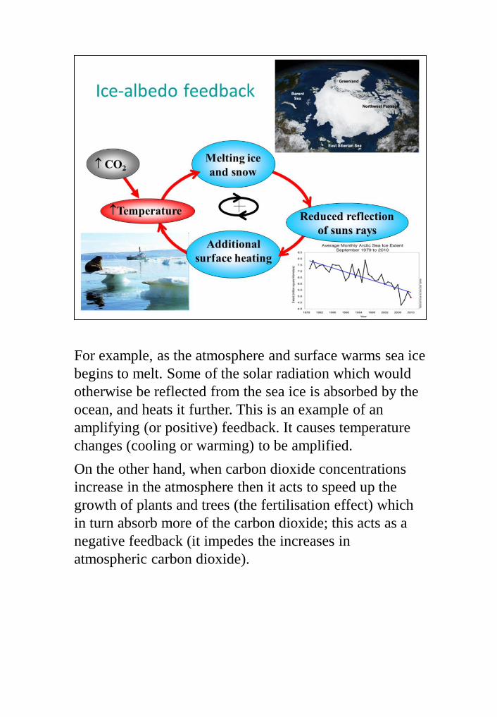
For example, as the atmosphere and surface warms sea ice
begins to melt. Some of the solar radiation which would
otherwise be reflected from the sea ice is absorbed by the
ocean, and heats it further. This is an example of an
amplifying (or positive) feedback. It causes temperature
changes (cooling or warming) to be amplified.
On the other hand, when carbon dioxide concentrations
increase in the atmosphere then it acts to speed up the
growth of plants and trees (the fertilisation effect) which
in turn absorb more of the carbon dioxide; this acts as a
negative feedback (it impedes the increases in
atmospheric carbon dioxide).

21
The strongest positive (amplifying) feedback that is
known to operate involves the invisible gaseous water
vapour which fills the atmosphere. As the atmosphere
warms it will also be able to ‘hold’ more water vapour.
Water vapour itself is a very powerful greenhouse gas,
and the water vapour feedback is one of the better
understood and most powerful positive feedbacks which
roughly doubles the amount of warming or cooling caused
by a radiative forcing compared to the case in which no
water vapour feedback operated.

22
There are many of these feedbacks, both positive and
negative, which we do not fully understand. This lack of
understanding is the main cause of the uncertainty in
climate response to a particular emissions scenario of the
future; this applies in particular to changes in clouds
which we will return to later.
To assess the accuracy of model predictions, the realism
of these feedback processes must be evaluated using
observations. For example, the water vapour feedback is
relatively well understood because it has been
demonstrated that water vapour near the surface in the
atmosphere increases by around 7% for every degrees C
rise in temperatures, in line with theoretical
considerations and with model projections.

Atmosphere-only and fully coupled climate models are
able to reproduce the observed variations in column
integrated water vapour and its dependence on surface
temperature over the oceans. Integrated water vapour is a
key variable since it affects:
- Precipitation over convective regions
- Radiative cooling of the atmosphere to the surface
- Global precipitation through a combination of the above
- Strongly positive water vapour feedback
Column integrated water vapour is mostly determined by
moisture in the lower troposphere while changes in
moisture throughout the middle and upper troposphere
are more important for water vapour feedback so it is
important to ensure that models accurately capture
changes in water vapour at these levels too.

Climate models (and weather forecast models) are
continually being evaluated and improved through
comparisons with observations and other types of models.
24

By prescribing scenarios in which atmospheric
constituents change in response to human-related
emissions and changes in natural forcing agents such as
the sun or volcanos, experiments can be made with
climate models to see how well they reproduce the past
climate and then what they project for future climate.

As we have already outlined, natural factors include a
chaotic variability of climate due largely to interactions
between atmosphere and ocean, changes in the output of
the Sun and changes in the optical depth of the
atmosphere from volcanic emissions. Climate models
have been driven by changes in all these natural factors,
and it simulates changes in global temperature shown by
the blue band in the slide above. This clearly does not
agree with observations, particularly in the period since
about 1970 when observed temperatures have risen by
about 0.5 °C, but those simulated from natural factors
have hardly changed at all.
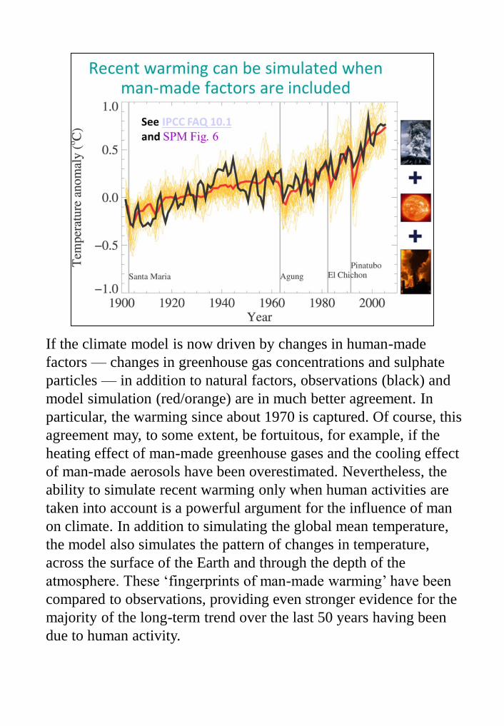
If the climate model is now driven by changes in human-made
factors — changes in greenhouse gas concentrations and sulphate
particles — in addition to natural factors, observations (black) and
model simulation (red/orange) are in much better agreement. In
particular, the warming since about 1970 is captured. Of course, this
agreement may, to some extent, be fortuitous, for example, if the
heating effect of man-made greenhouse gases and the cooling effect
of man-made aerosols have been overestimated. Nevertheless, the
ability to simulate recent warming only when human activities are
taken into account is a powerful argument for the influence of man
on climate. In addition to simulating the global mean temperature,
the model also simulates the pattern of changes in temperature,
across the surface of the Earth and through the depth of the
atmosphere. These ‘fingerprints of man-made warming’ have been
compared to observations, providing even stronger evidence for the
majority of the long-term trend over the last 50 years having been
due to human activity.
28
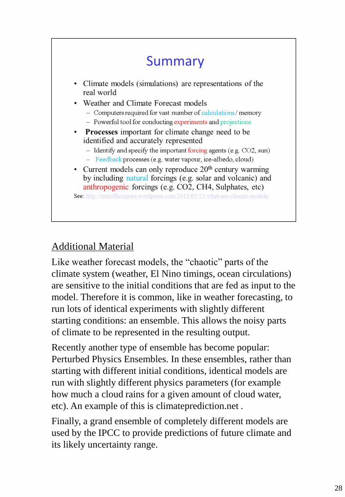
Additional Material
Like weather forecast models, the “chaotic” parts of the
climate system (weather, El Nino timings, ocean circulations)
are sensitive to the initial conditions that are fed as input to the
model. Therefore it is common, like in weather forecasting, to
run lots of identical experiments with slightly different
starting conditions: an ensemble. This allows the noisy parts
of climate to be represented in the resulting output.
Recently another type of ensemble has become popular:
Perturbed Physics Ensembles. In these ensembles, rather than
starting with different initial conditions, identical models are
run with slightly different physics parameters (for example
how much a cloud rains for a given amount of cloud water,
etc). An example of this is climateprediction.net .
Finally, a grand ensemble of completely different models are
used by the IPCC to provide predictions of future climate and
its likely uncertainty range.