NUREG/CR-3046, Vol. 4, 'COBRA/TRAC -A Thermal-Hydraulics ... · NUREG/CR-3046 PNL-4385 Vol. 4 R4...
232
NUREG/CR-3046 PNL-4385 Vol. 4 COBRA/TRAC - A Thermal-Hydraulics Code for Transient Analysis of Nuclear Reactor Vessels and Primary Coolant Systems Developmental Assessment and Data Comparisons Prepared by M. J. Thurgood, T. E. Guidotti, G. A. Sly, J. M. Kelly, R. J. Kohrt, K. R. Crowell, C. A. Wilkins, J. M. Cuta, S. H. Bian Pacific Northwest Laboratory Operated by Battelle Memorial Institute Prepared for U.S. Nuclear Regulatory Commission
Transcript of NUREG/CR-3046, Vol. 4, 'COBRA/TRAC -A Thermal-Hydraulics ... · NUREG/CR-3046 PNL-4385 Vol. 4 R4...

NUREG/CR-3046PNL-4385Vol. 4
COBRA/TRAC - A Thermal-HydraulicsCode for Transient Analysisof Nuclear Reactor Vesselsand Primary Coolant SystemsDevelopmental Assessment and Data Comparisons
Prepared by M. J. Thurgood, T. E. Guidotti, G. A. Sly,J. M. Kelly, R. J. Kohrt, K. R. Crowell,C. A. Wilkins, J. M. Cuta, S. H. Bian
Pacific Northwest LaboratoryOperated byBattelle Memorial Institute
Prepared forU.S. Nuclear RegulatoryCommission

NOTICE
This report was prepared as an account of work sponsored by an agency of the United StatesGovernment. Neither the United States Government nor any agency thereof, or any of theiremployees, makes any warranty, expressed or implied, or assumes any legal liability of re-sponsibility for any third party's use, or the results of such use, of any information, apparatus,product or process disclosed in this report, or represents that its use by such third party wouldnot infringe privately owned rights.
Availability of Reference Materials Cited in NRC Publications
Most documents cited in NRC publications will be available from one of the following sources:
1. The NRC Public Document Room, 1717 H Street, N.W.Washington, DC 20555
2. The NRC/GPO Sales Program, U.S. Nuclear Regulatory Commission,Washington, DC 20555
3. The National Technical Information Service, Springfield, VA 22161
Although the listing that follows represents the majority of documents cited in NRC publications,it is not intended to be exhaustive.
Referenced documents available for inspection and copying for a fee from the NRC Public Docu-ment Room include NRC correspondence and internal NRC memoranda; NRC Office of Inspectionand Enforcement bulletins, circulars, information notices, inspection and investigation notices;Licensee Event Reports; vendor reports and correspondence; Commission papers; and applicant andlicensee documents and correspondence.
The following documents in the NUREG series are available for purchase from the NRC/GPO SafesProgram: formal NRC staff and contractor reports, NRC-sponsored conference proceedings, andNRC booklets and brochures. Also available are Regulatory Guides, NRC regulations in the Code ofFederal Regulations, and Nuclear Regulatory Commission Issuances.
Documents available from the National Technical Information Service include NUREG seriesreports and technical reports prepared by other federal agencies and reports prepared by the AtomicEnergy Commission, forerunner agency to the Nuclear Regulatory Commission.
Documents available from public and special technical libraries include all open literature items,such as books, journal and periodical articles; and transactions. Federal Register notices, federal andstate legislation, and congressional reports can usually be obtained from these libraries.
Documents such as theses, dissertations, foreign reports and translations, and non-N RC conferenceproceedings are available for purchase from the organization sponsoring the publication cited.
Single copies of NRC draft reports are available free upon written request to the Division of Tech-nical Information and Document Control, U.S. Nuclear Regulatory Commission, Washington, DC20555.
Copies of industry codes and standards used in a substantive manner in the NRC regulatory processare maintained at the NRC Library, 7920 Norfolk Avenue, Bethesda, Maryland, and are availablethere for reference use by the public. Codes and standards are usually copyrighted and may bepurchased from the originating organization or, if they are American National Standards, from theAmerican National Standards Institute, 1430 Broadway, New York, NY 10018.
GPO Printed copy price: - $7.50

NUREG/CR-3046PNL-4385Vol. 4R4
COBRA/TRAC- A Thermal-HydraulicsCode for Transient Analysisof Nuclear Reactor Vesselsand Primary Coolant SystemsDevelopmental Assessment and Data Comparisons
Manuscript Completed: November 1982Date Published: March 1983
Prepared byM. J. Thurgood, T. E. Guidotti, G. A. Sly,J. M. Kelly, R. J. Kohrt, K. R. CrowellC. A. Wilkins, J. M. Cuta, S. H. Bian
Pacific Northwest LaboratoryRichland, WA 99352
Prepared forDivision of Accident EvaluationOffice of Nuclear Regulatory ResearchU.S. Nuclear Regulatory CommissionWashington, D.C. 20555NRC FIN B2391


ABSTRACT
The COBRA/TRAC computer program has been developed to predict thethermal-hydraulic response of nuclear reactor primary coolant systems to smalland large break loss-of-coolant accidents and other anticipated transients.The code solves the compressible three-dimensional, two-fluid, three-fieldequations for two-phase flow in the reactor vessel. The three fields are thevapor field, the continuous liquid field, and the liquid drop field. A five-equation drift flux model is used to model fluid flow in the primary systempiping, pressurizer, pumps, and accumulators. The heat generation rate of thecore is specified by input and no reactor kinetics calculations are includedin the solution. This volume documents the major data comparisons made withCOBRA/TRAC during the process of code development. These data comparisonswere extremely useful in detecting programming errors and definingdeficiencies in the code's physical models. The data comparisons presented inthis volume document the results obtained on developmental versions of thecode. A separate document will be released at a later date containing datacomparisons run on the final released version of the code.
iii


CONTENTS
ACKNOWLEDGEMENTS .............. .................................... . xix
l.O INTRODUCTION ............... o..... ooo................ ........ ...... 1.
2.0 DATA COMPARISONS PERFORMED WITH DEVELOPMENTAL VERSIONS OFCOBRA/TRAC -................... ...... ..... .... ... .... . ...... 2.1
2.1 DARTMOUTH COUNTERCURRENT FLOW TUBE FLOODINGEXPERIMENTS..... ..... . . . . ... . . . .. . . ......... o - o - o - o - - 2.3
2.1.1 Description of Experiment ....... . .......... ..... 2.3
2.1.2 COBRA/TRAC Model ... o .......... .. o.o...o....... .. .. 2.4
2.1.3 Discussion of Results.............................2.6
2.2 NORTHWESTERN UNIVERSITY ORIFICE PLATE FLOODINGEXPERIMENT*** - -*..... ...... ....... .... .... .... o.o .. .. 2.8
2.2.1 Description of Experiment. .................. .. ... . 2.8
2.2.2 COBRA/TRAC Model Description........... ............ 2.9
2.2.3 Discussion of Results...... ... ..... ..... .... . ... 2.10
2.3. CREARE 1/15th SCALE DOWNCOMER ECC BYPASSEXPERIMENTSo ........... o o.................... o....... ..... 2.11
2.3.1 Description of Experiment. ..... ................. 2.12
2.3.2 COBRA/TRAC Model Description.. ..... ... ............ 2.13
2.3.3 Discussion ofResults. ........................ o...2.14
2.4 BATTELLE COLUMBUS 2/15ths SCALE DOWNCOMERTRANSIENT ECC BYPASS EXPERIMENT......................... 2.15
2.4.1 Description of Experiment........... ............ 2.18
2.4.2 COBRA/TRAC Model Description........... ..... ..... 2.19
2.4.3 Discussion of Results.. .......................... 2.22
2.5 FEBA FORCED BOTTOM REFLOOD EXPERIMENT.......... ........ 2.25
2.5.1 Description of Experiment ................... o.... 2.25
2.5.2 COBRA/TRAC Model Description.....................2.29
v

2.5.3 Discussion of Results.............. ....... 2.31
2.6 FLECHT LOW FLOODING RATE COSINE TEST SERIES ............. 2.37
2.6.1 Description of Experiment........................ 2.37
2.6.2 COBRA/TRAC Model Description .............. 239
2.6.3 Discussion of Results ............................ 2.43
2.7 STANDARD PROBLEM NO. 9 .................................. 2.50
2.7.1 Experimental Descriptiobn ......................... 2.57
2.7.2 COBRA/TRAC Model Description...................... 2.60
2.7.3 Discussion of Results........* ..................2.62
2.8 NRU NUCLEAR FUEL ROD FORCED REFLOOD EXPERIMENT .......... 2.74
2.8.1 Experimental Description .......................... 2.74
2.8.2 COBRA/TRAC Model Description ............. . ....... 2.78
2.8.3 Discussion of Results ............................ 2.80
2.9 PKL GRAVITY REFLOOD EXPERIMENT K9 ...................... 2.91
2.9.1 Description of Experiment ...... 2.........2.91
2.9.2 COBRA/TRAC Model Description ..................... 2.93
2.9.3 Discussion of Results ............................ 2..95
2.10 CYLINDRICAL CORE TEST FACILITY GRAVITY REFLOOD ........ 2.105
2.10.1 Description of Experiment ..................... 2.105
2.10.2 COBRA/TRAC Model Description .................. 2.108
2.10.3 Discussion of Results ......................... 2.108
2.11 NORTHWESTERN UNIVERSITY COUNTERCURRENT FLOWFILM CONDENSATION EXPERIMENT .......................... 2.122
2.11.1 Description of Experiment ...................... 2.122
2.11.2 COBRA/TRAC Model Description .................. 2.124
2.11.3 Discussion of Results ......................... 2.126
vi

2.12 RPI FLAT PLATE PHASE DISTRIBUTION EXPERIMENT ........... 2.127
2.12.1 Description of Experiment ...................... 2.127
2.12.2 COBRA/TRAC Model Description .................. 2.129
2.12.3 Discussion of Results ......................... . 2.129
2.13 BENNETT TUBE CRITICAL HEAT FLUX EXPERIMENTS ............ 2.136
2.13.1 Description of Experiment ..................... 2.136
2.13.2 COBRA/TRAC Model Description .................. 2.137
2.13.3 Discussion of Results ......................... 2.138
2.14 FRIGG FORCED CONVECTION TESTS ........... ............. 2.151
2.14.1 Description of Experiment ..................... 2.151
2.14.2 COBRA/TRAC Model Description .................. 2.152
2.14.3 Discussion of Results .................... *.... 2.153
2.15 FRIGG NATURAL CIRCULATION TESTS .............. ......... 2.157
2.15.1 Description of Experiment ..................... 2.157
2.15.2 COBRA/TRAC Model Description .................. 2.159
2..15.3 Discussion of Results ......................... 2.159
2.16 SEMISCALE MOD3 TEST S-07-6 ............................. 2.164
2.16.1 Description of Experiment ..................... 2.164
2.16.2 COBRA/TRAC Model Description .................. 2.165
2.16.3 Discussion of Results ...... .................... 2.169
2.17 SEMISCALE MOD2A TEST S-UT-2 ............................ 2.173
2.17.1 Description of Experiment. ................ .... 2.173
2.17.2 COBRA/TRAC Model Description .................. 2.176
2.17.3 Discussion of Results ....................... 2.178
2.18 WESTINGHOUSE UPPER HEAD DRAIN TEST ..................... 2.188
2.18.1 Description of Experiment .... .. ... ..... .... 2.188
vii
2.18.2 COBRA/TRAC Model Description .................. 2.189
2.18.3 Discussion of Results ......... ..... ...... 2.190
REFERENCES ........ .............................. ........... .R.1
APPENDIX A ............................................... A.1
viii

FIGURES
2.1-1 Experimental Setup for Flooding in Large Tubes ................... 2.5
2.1-2 Liquid Penetration in 2-in. Tube ................................ 2.7
2.1-3 Liquid Penetration in 10-in. Tube ............................... 2.7
2.2-1 COBRA/TRAC Model of Northwestern University CCFL ExperimentalFacility ....................................... . ................ 2.9
2.2-2 Liquid Penetration - DBUBMAX = Hydraulic Diameter .............. 2.11
2.2-3 Liquid Penetration - DBUBMAX = 2*(hydraulic diameter) .......... 2.12
2.3-1 Schematic of CREARE Downcomer Vessel ........................... 2.13
2.3-2 COBRA/TRAC Model of CREARE Downcomer ........................... 2.14
2.3-3 Downcomer Penetration Curve - Saturated ECC Water at 30 GPM.....2.16
2.3-4 Downcomer Penetration Curve - Saturated ECC Water at 120 GPM...2.16
2.3-5 Downcomer Penetration Curve - Subcooled ECC Water at 30 GPM .... 2.17
2.3-6 Downcomer Penetration Curve - Subcooled ECC Water at 120 GPM...2.17
2.4-1 Diagram of Battelle Columbus 2/15th Scale Downcomer Vessel ..... 2.19
2.4-2 COBRA/TRAC Model of BCL Downcomer ............................. 2.20
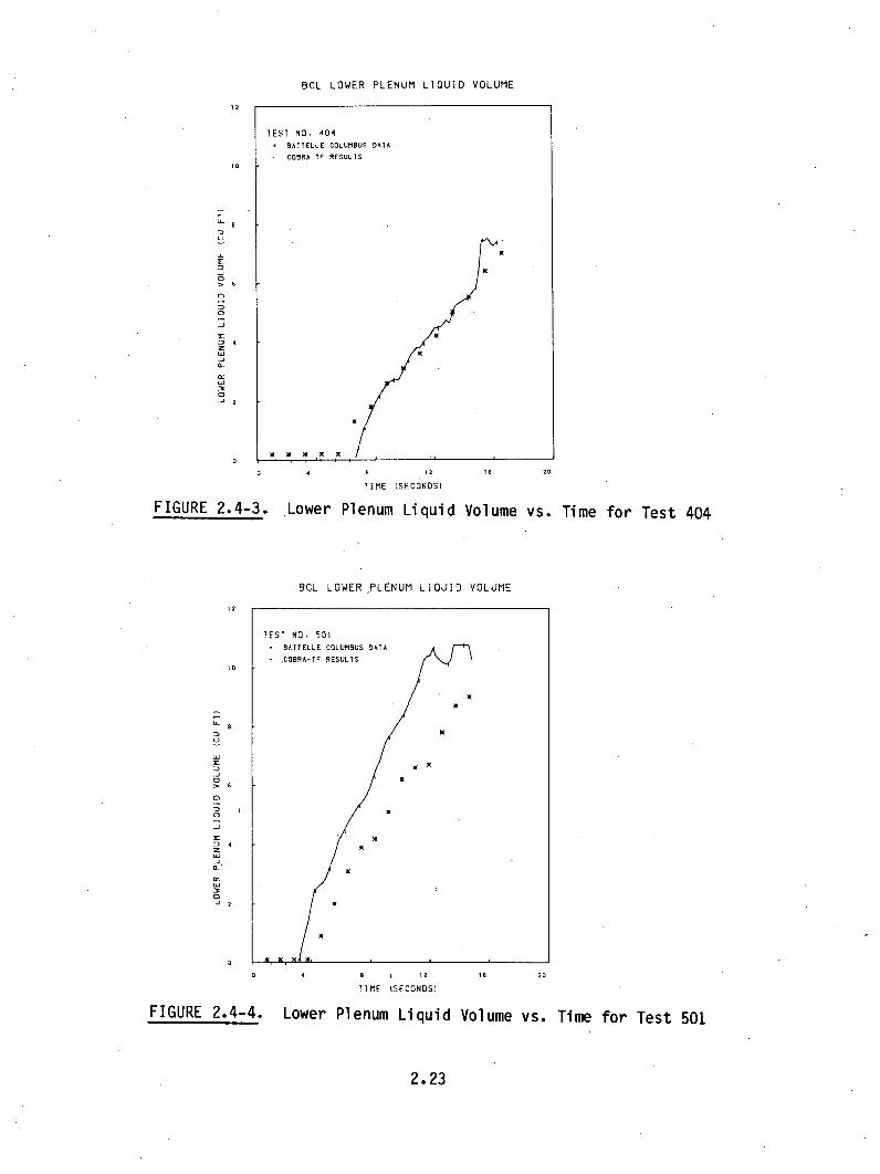
2.4-3 Lower Plenum Liquid Volume vs. Time for Test 404 ............... 2.23
2.4-4 Lower Plenum Liquid Volume vs. Time for Test 501 ............... 2.23
2.4-5 Lower Plenum Pressure vs. Time for Test 501 .................... 2.24
2.4-6 Net Condensation Rate in the Vessel vs. Time for Test 404 ...... 2.24
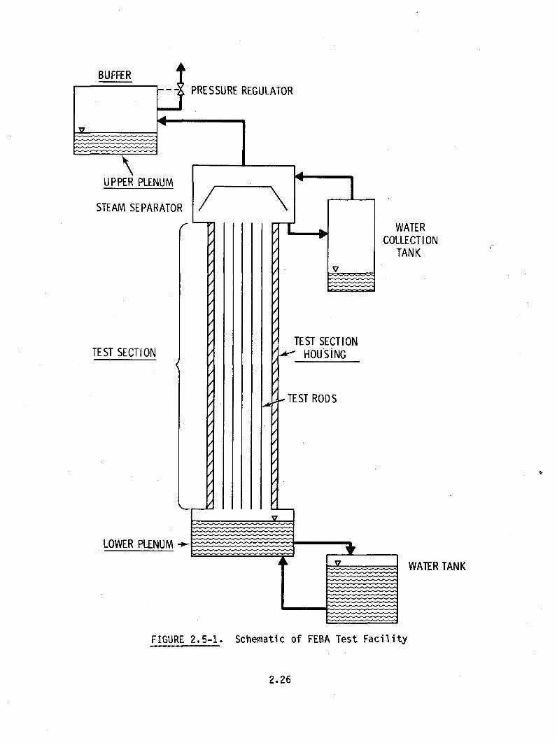
2.5-1 Schematic of FEBA Test Facility ................................ 2.26
2.5-2 Cross Section of FEBA 5x5 Test Section Bundle RepresentativeHeater Rod ..................................................... 2.28
2.5-3 Axial Power Profile and Grid Spacer Locations for FEBA
Test Section ........................... ............... ....... 2.28
2.5-4 Power Decay Curve for FEBA Test Run 216 ........................ 2.29
2.5-5 COBRA/TRAC Model of FEBA.Test Section .......................... 2.30
2.5-6 COBRA/TRAC Initial Rod Temperatures vs. Axial Position ......... 2.32
ix
2.5-7 Test Section Axial Power Profile and COBRA/TRAC Model of theAxial Power Profile ............................................ 2.32
2.5-8 COBRA/TRAC Predicted Rod Temperatures at 0.8m for FEBATest 216 ........................... ............................ 2.33
2.5-9 COBRA/TRAC Predicted Rod Temperatures at 1.3m for FEBATest 216 ....................................................... 2.33
2.5-10 COBRA/TRAC Predicted Rod Temperatures at 1.9m for FEBATest 216 ....................................................... 2.34
2.5-11 COBRA/TRAC Predicted Rod Temperatures at 2.4m for FEBATest 216 ....................................................... 2.34
2.5-12 COBRA/TRAC Predicted Rod Temperatures at 3.0m for FEBATest 216 ....................................................... 2.35
2.5-13 COBRA/TRAC Predicted Rod Temperatures at 3.5m for FEBATest 216 ............................... ....... ................ 2.35
2.5-14 Collapsed Liquid Level vs. Time for FEBA Test 216 .............. 2.36
2.6-1 FLECHT Test Bundle Cross Section ............................... 2.38
2.6-2 FLECHT Test Section Axial Power Profile and Grid Elevations .... 2.39
2.6-3 COBRA/TRAC Model of FLECHT Test Section ........................ 2.41
2.6-4 Temperature at 2-ft Elevation - FLECHT 00904 ................... 2.44
2.6-5 Temperature at 4-ft Elevation - FLECHT 00904 ................... 2.44
2.6-6 Temperature at 6-ft Elevation - FLECHT 00904 ................... 2.45
2.6-7 Temperature at 7-ft Elevation - FLECHT 00904 ................... 2.45
2.6-8 Temperature at 9-ft Elevation - FLECHT 00904 ................... 2.46
2.6-9 Temperature at 10-ft Elevation - FLECHT 00904 ................ 2.46
2.6-10 Vapor Fraction at 0 to 2-ft Elevation for FLECHT 00904 ......... 2.47
2.6-11 Vapor Fraction at 2 to 4-ft Elevation for FLECHT 00904 ........ 2.47
2.6-12 Vapor Fraction at 4 to 6-ft Elevation for FLECHT 00904 ......... 2.48
2.6-13 Vapor Fraction at 6 to 8-ft Elevation for FLECHT 00904 ......... 2.48
2.6-14 Vapor Fraction at 8 to 10-ft Elevation for FLECHT 00904 ........ 2.49
2.6-15 Vapor Fraction at 10 to 12-ft Elevation for FLECHT 00904 ....... 2.49
X

2.6-16
2.6-17
2.6-18
2.6-19
2.6-20
2.6-21
2.6-22
2.6-23
2.6-24
2.6-25
2.6-26
2.6-27
Temperature at
Temperature at
Temperature at
Temperature at
Temperature at
Temperature at
Temperature at
Vapor Fraction
Vapor Fraction
Vapor Fraction
Vapor Fraction
Vapor Fraction
2-ft Elevation--FLECHT 04444 .................... 2.51
4-ft Elevation--FLECHT 04444 .................... 2.51
6-ft Elevation--FLECHT 04444 .................... 2.52
7-ft Elevation--FLECHT 04444 .................... 2.52
8-ft Elevation--FLECHT 04444 .................... 2.53
9-ft Elevation--FLECHT 04444 .................... 2.53
10-ft Elevation..FLECHT 04444 ................... 2.54
at 0 to 2-ft ElIevation--FLECHT 04444 ............ 2.54
at 2 to 4-ft Elevation--FLECHT 04444 ............ 2.55
at 4 to 6-ft Elevation--FLECHT 04444 ............ 2.55
at 6 to 8-ft Elevation--FLECHT 04444............2.56
at 8 to 10-ft Elevation--FLECHT 04444 ........... 2.56
2.6-28 Vapor Fraction at 10 to 12-ft Elevation--FLECHT 04444 .......... 2.57
2.7-1 FLECHT-SEASET Bundle Cross-Section ............................. 2.58
2.7-2 FLECHT-SEASET Axial Power Profile and Grid Locations ........... 2.59
2.7-3 COBRA/TRAC Model of FLECHT-SEASET for Standard Problem No. 9...2.61
2.7-4 Temperatures at 2-ft Elevation for Low Reflood Rate(Test 31805) ................................................... 2.63
2.7-5 Temperatures at 4-ft Elevation for Low Reflood Rate(Test 31805) ................................................... 2.63
2.7-6 Temperatures at 6-ft Elevation for Low Reflood Rate(Test 31805) ................................................... 2.64
2.7-7 Temperatures at 11-ft Elevation for Low Reflood Rate(Test 31805) ................................................... 2.64
2.7-8 Temperatures at 11'ft Elevation for Low Reflood Rate
(Test 31805) ........ ........................................... 2.65
2.7-9 Vapor Fraction at 0 to 1-ft Elevation for Low Reflood Rate(Test 31805) ................................................... 2.65
2.7-10 Vapor Fraction at 1 to 2-ft Elevation for Low Reflood Rate.(Test 31805) ................................................... 2.66
xi

2.7-11 Vapor(Test
2.7-12 Vapor(Test
2.7-13 Vapor(Test
2.7-14 Vapor(Test
2.7-15 Vapor(Test
2.7-16 Vapor(Test
2.7-17 Vapor(Test
2.7-18 Vapor(Test
2.7-19 Vapor(Test
2.7-20 Vapor(Test
Fraction at 2- to 3-ft Elevation for Low Reflood Rate31805) at 3 to 4 Elvto.o.o................. .... 2.66
Fraction at 3 to 4-ft Elevation for Low Reflood Rate31805)o ..............at 5to.t........ E a n r w f d2t67
Fraction at 4 to 5-ft Elevation for Low Reflood Rate31805) .........a to8-...ft.Ele. ....vatio...... f wodRee i2.67
Fraction at 5 to 6-ft Elevation for Low Reflood Rate31805) .................t....... 9 ................ v..... ... 2.68
Fraction at 6 to 7-ft Elevation for Low Reflood Rate31805) ...... .................................... ....... 2.68
Fraction at 7 to 8-ft Elevation for Low Reflood Rate31805) .................. o*.................. ... ............ 2.69
Fraction at 8 to 9-ft Elevation for Low Reflood Rate31805) ..... o......... . . . . . . . . . . . . . . . . . . .2 6
Fraction at 9 to lO-ft Elevation for Low Reflood Rate31805) ............. .. ............... ...* ... e ... o . *... .... ... 2.70
Fraction at 10 to 11-ft Elevation for Low Reflood Rate31805) ............. e......... ... ... .... o...............*.... 2.70
Fraction at 11 to 12-ft Elevation for Low Reflood Rate31805) ........... 0... ........ ...... .. .... 0........ . *... ... .2.71
2.7-21 Temperatures at 2-ft Elevation for High Reflood Rate(Test 31701) ..... .............................................. 2.71
2.7-22 Temperatures at 4-ft Elevation for High Reflood Rate(Test 31701) .................. ................................ 2.72
2.7-23 Temperatures at 6-ft Elevation for High Reflood Rate(Test 31701) ...................... .............................. 2.72
2.7-24 Temperatures at lO-ft Elevation for High Reflood Rate(Test 31701) ................................................... 2.73
2.7-25 Temperatures at 11-ft Elevation for High Reflood Rate(Test 31701) ........................... ................ ... ..... 2.73
2.8-1 Vertical Test Train Configuration for NRU Reflood Experiments..2.75
2.8-2 NRU Test Bundle Cross-Section .................................. 2.76
2.8-3 COBRA/TRAC Model of NRU Test Section ................ . ...... 2.79
2.8-4 Temperatures at the 1.12-ft Elevation (Test PTH110) ............ 2.81
xii
2.8-5
2.8-6
2.8-7
2.8-8
2.8-9
2.8-10
2.8-11
2.8-12
2.8-13
2.8-14
2.8-15
2.8-16
2.8-17
2.8-18
2.8-19
2.8-20
2.9-1
2.9-2
2.9-3
2.9-4
2.9-5
2.9-6
2.9-7
2.9-8
2.9-9
2.9-10
Temperatures
Temperatures
Temperatures
Temperatures
Temperatures
Temperatures
Temperatures
Temperatures
Temperatures
Temperatures
Temperatures
Temperatures
.Temperatures
Temperatures
Temperatures
at the 3.0-ft Elevation (Test PTH110) ............. 2.81
at the 4.0-ft Elevation (Test PTH110) ............. 2.82
at the 5.0-ft Elevation (Test PTH110) ............. 2.82
at the 6.0-ft Elevation (Test PTH110) ............. 2.83
at the 7-ft Elevation (Test PTH110) ............... 2.83
at the 8.0-ft Elevation (Test PTH110) ............. 2.84
at the 10.0-ft Elevation (Test PTH110)...........2.84
at the 1.12-ft Elevation (Test TH214)............. 2.86
at the 3.0-ft Elevation (Test TH214).............. 2.86
at the 4.0-ft Elevation (Test TH214) ... o..........2.87
at the 5.0-ft Elevation (Test TH214). ........... 2.87
at the 6.0-ft Elevation (Test TH214).............. 2.88
at the 7-ft Elevation (Test TH214)................2.88
at the 8.0-ft Elevation (Test TH214).............. 2.89
at the 10.0-ft Elevation (Test TH214)............. 2.89
Collapsed Liquid Level vs. Time (Test TH214) ................... 2.90
Diagram of PKL System .......................................... 2.92
COBRA/TRAC Model of PKL Test Facility..•........................ 2.94
Schematic of COBRA/TRAC Model of PKL Pressure Vesseland Downcomer . . . . . ........................... ... ##.......... 2.94
Pressure in the Upper Plenum (Channels 5-8) .................... 2.96
Pressure in the Break Pipe..................................... 2.96
Collapsed Water Level in the Core .............................. 2.98
Flow Rate in the Downcomer (Averaged Over Length ofChannel 10) .................................................... 2.98
Flow Rate in the Downcomer at the Lower Boundary Node .......... 2.99
Rod Surface Temperature at Level 1 ............................. 2.99
Rod Surface Temperature at Level 2 ............................ 2.100
xiii

2.9-11 Rod Surface Temperature at Level 3 ............................ 2.100
2.9-12 Rod Surface Temperature at Level 4 ............................. 2.101
2.9-13 Rod Surface Temperature at Level 42 ........................... 2.101
2.9-14 Rod Surface Temperature at Level 51 ........................... 2.102
2.9-15 Rod Surface Temperature at Level 7 ............................ 2.102
2.9-16 Quench Front Envelope .......................................... 2.103
2.9-17 Void Fraction in the Core, (Channel 3, Nodes 3-5) ............. 2.103
2.9-18 Void Fraction in the Core, (Channels 3-4, Node 5-9,2) ......... 2.104
2.9-19 Void Fraction in the Core ..................................... .2.104
2.10-1 Schematic of Cylindrical Core Test Facility ...... ............ 2.106
2.10-2 Diagram of CCTF Pressure Vessel ............................... 2.109
2.10-3 Cross-Section of CCTF Core ..................................... 2.110
2.10-4 Axial Power Profile and Thermocouple Elevations for Heater Rodsin CCTF Core .................................................. 2.111
2.10-5 Schematic of COBRA/TRAC Model of CCTF ......................... 2.113
2.10-6 Vessel Mesh for CCTF .......................................... 2.113
2.10-7 Differential Pressure in the Lower Plenum ..................... 2.114
2.10-8 Differential Pressure Between the 0 and 2-ft Elevationsin the Core ................................................... 2.114
2.10-9 Differential Pressure Between 2 and 4-ft Elevationsin the Core ................................................... 2.115
2.10-10 Differential Pressure Between 4 and 5-ft Elevationsin the Core .................. .. ........ ........... 2.115
2.10-11 Differential Pressure Between 6 and 8-ft Elevationsin the rere in.the..... Uppe .. .................... 2.116
2.10-12 Differential Pressure Between 8 and lO-ft Elevations.in the Core ... ... .... .... o. .......... .... ... .... .... ... ... 2.116
2.10-13 Differential Pressure Between 10 and 12-ft Elevationsin the Core .........- o........ o............... ................ oo 2.117
2.10-14 Differential Pressure in the Upper Plenum ............. Io.o.....2.17
xiv

2.10-15 Temperature at 0.38 m Elevation .............................. 2.118
2.10-16 Temperature at 1.015 m Elevation ............................. 2.118
2.10-17 Temperature at 1.83 m Elevation .............................. 2.119
2.10-18 Temperatureat2.44m Elevation .............................. 2.119
2.10-19 Temperature at 3.05 m Elevation .............................. 2.120
2.11-1 Vertical Test Apparatus for CounterCurrent Flow FilmCondensation Experiments ............... . ..................... 2.123
2.11-2 COBRA/TRAC Model for NWU CCFF Condensation Tests ............. 2.125
2.11-3 Steam Flow Rate as a Function of Axial Position ........... *...2.126
2.12-1 RPI Phase Separation Experimental Apparatus .................. 2.128
2.12-2 COBRA/TRAC Model of the RPI Phase Separation ExperimentTest Section . . . . . . . . . . . . . . . . .*. . . . .. ..2.130
2.12-3 Void Distribution for RPI Test #8 Predicted by COBRA/TRAC withoutthe Turbulence Model ......................................... 2.131
2.12-4 Void Distribution for RPI Test #10 Predicted by COBRA/TRAC withoutthe Turbulence Model ....................................... o.2.132
2.12-5 Void Distribution for RPI Test #8 Predicted by COBRA/TRAC withthe Turbulence Model ..... . .............................................. 2.133
2.12-6 Void Distribution for RPI Test #10.Predicted by COBRA/TRAC withthe Turbulence Model ............................................ 2.134
2.13-1 COBRA/TRAC Mesh for Bennett Tests ............................ 2.138
2.13-2 Entrained Liquid in Bennett Test No. 5373 ......... ........... 2.140
2.13-3 Bennett Test Critical Heat Flux vs. Equilibrium Quality(at Mass Flux = 2.84x10⁶ lbm/hr-ft 2 ) ........................ , 2.141
2.13-4 Bennett Test Critical 9eat Flux vn. Equilibrium Quality(at Mass Flux = 1.OxlO lbm/hr-ft) ......................... 2.141
2.13-5 Bennett Test Critical Hgat Flux vs, Equilibrium Quality(at Mass Flux = 0.49xi0 lbm/hr-ft ) ......................... 2.142
2.13-6 Bennett Test Critical Heat Flux vs. Equilibrium Quality
(at Mass Flux 5 0.29xi06 Tbm/hr-ft2) ......................... 2.142
2.13-7 Bennett Test 5359 Axial Temperature Profile .................. 2.145
2.13-8 Bennett Test 5336 Axial Temperature Profile .................. 2.145
xv
2.13-9 Bennett Test 5273 Axial Temperature Profile ................... 2.146
2.13-10 Bennett Test 5250 Axial Temperature Profile .................. 2.146
2.13-11 Bennett Test 5294 Axial Temperature Profile ................ 2.147
2.13-12 Bennett Test 5313 Axial Temperature Profile .................. 2.147
2.13-13 Bennett Test 5310 Axial Temperature Profile .................. 2.148
2.13-14 Bennett Test 5379 Axial Temperature Profile .................. 2.148
2.13-15 Bennett Test 5397 Axial Temperature Profile .................. 2.149
2.14-1 Simplified Diagram of FRIGG Forced Convection Loop ........... 2.152
2.14-2 COBRA/TRAC Model of FRIGG Forced Convection Loop ............. 2.153
2.14-3 FRIGG Forced Convection Test 313018 .......................... 2.155
2.14-4 FRIGG Forced Convection Test 313020 ........................... 2.155
2.14-5 FRIGG Forced Convection Test 313016 .......................... 2.156
2.15-1 Simplified Diagram of FRIGG Natural Circulation Loop ......... 2.158
2.15-2 COBRA/TRAC Model of FRIGG Natural Circulation Loop ........... 2.160
2.15-3 FRIGG Natural Circulation Test 313030 ........................ 2.162
2.15-4 FRIGG Natural Circulation Test 313034 ........................ 2.162o
2.15-5 FRIGG Natural Circulation Test 313037..................... 2.163
2.15-6 FRIGG Natural Circulation Mass Velocities.................... 2.163
2.16-1 COBRA/TRAC Model of Semiscale MOD3 System .................... 2.166
2.16-2 COBRA/TRAC Model of Semiscale Pressure Vessel and Downcomerfor Test S-07-6 .. .................... o ... - .................... 2.168
2.16-3 Upper Plenum Pressure ................ .............. . ........ . 2.170
2.16-4 Density at Top of Core ......... & ................ ........ .... . .2.170
2.16-5 Density in Upper Head ....................................... 2.171
2.17-1 Semiscale MOD2A System for Small Break LOCA ................. 2.174
2.17-2 Detail of Small Break Orifice in Test S-UT-2 ................. 2.175
2.17-3 COBRA/TRAC Model of Semiscale MOD2A System .................... 2.177
xvi

2.17-4 COBRA/TRAC Model of Semiscale Pressure Vessel and Downcomerfor Test S-UT-2 .............................................. 2.179
2.17-5 COBRA/TRAC Noding of Break Nozzle ............................ 2.180
2.17-6 System Pressure ................................................ 2.182
2.17-7 Collapsed Liquid Level in Semiscale Downcomer Pipe.......... 2.183
2.17-8 Collapsed Liquid Level in Semiscale Core ..................... 2.183
2.17-9 Collapsed Liquid Level in Upper Head ......................... 2.184
2.17-10 Upper Head Fluid Temperature ................................. 2.184
2.17-11 Rod Temperature at the Core Mid-Plane ........................ 2.185
2.17-12 Rod Temperature Near Top of Core ............................. 2.185
2.18-1 COBRA/TRAC Model of Westinghouse Upper Head Test Section ..... 2.190
2.18-2 Westinghouse Drain Test #5; Upper Head Liquid Levelvs. Time ..................................................... 2.191
2.18-3 Westinghouse Drain Test #5; Fluid Temperature at Top of SupportColumns Westinghouse.rain.Test.#5 P at T of.Guide..u.....2.191
2.18-4 Westinghouse Drain Test #5; Pressure at Top of Guide Tube .... 2.192
xvii

TABLES
2.1 Battelle Columbus 2/15th Scale Downcomer Test Conditions ......... 2.21
2.2 Reverse Core Steam Flow Rate Ramps for BCL 2/15th ScaleDowncomer Tests .................................................. 2.21
2.3 Boundary Conditions for FEBA Test 216 ............................ 2.29
2.4 Initial Conditions for FLECHT Cosine Series Tests ................ 2.40
2.5 FLECHT Initial Cladding Temperatures .............................. 2.42
2.6 Test Parameters for Standard Problem"No. 9 ....................... 2.59
2.7 Initial Design Parameters for NRU Tests PTH110 and TH214 ......... 2.77
2.8 Component Scaled Dimensions for Cylindrical CoreTest Facility ................................................... 2.107
2.9 Summary of Conditions for CCTF Test C1-2.............. ...... 2.112
2.10 Execution Speeds and Average Time Steps for Calculations of RPI
Phase Separation Tests ....... . ................ o .... *.... .. .... 2.136
2.11 Summary of Bennett Test Conditions and Results of Dryout
Point Calculations .....ry ofF ocd.ovcto .es.od................. 2.139
2.12 Summary of FRIGG Forced Convection Test Conditions .............. 2.154
2.13 Summary of FRIGG Natural Circulation Test Conditions ............ 2.160
2.14 Initial Conditions for Semiscale Test S-07-2 .................... 2.1692.15 Initial Conditions for Semiscale Test S-UT-2 .................... 2.182
xviii

ACKNOWLEDGEMENTS
COBRA/TRAC is the result of the efforts of a number of people. We wish
to acknowledge the main contributors and to express our appreciation to those
who have offered their advice and suggestions.
The main contributors to the) program are listed below.
Fluid Dynamics:
Heat Transfer
Turbulence Model
Graphics and Programming:
Simulations:
One-Dimensional Components
and Code Architecture:
M. J. Thurgood, T. L. George, and
T. E. Guidotti
J. M. Kelly, R. J. Kohrt
K.'R. Crowell
A. S. Koontz
K. L. Basehore, S. H. Bian, J. M. Cuta,
R. J. Kohrt, G. A. Sly and
C. A. Wilkins
Members of the TRAC-PlA Code Development
Group at LANL
We wish to thank Dr. S. Fabic of the U.S. Nuclear Regulatory Commission
for his patience, support and suggestions during this large undertaking. We
also wish to thank Drs. Tong, Shotkin, Han and Zuber of the U.S. Nuclear
Regulatory Commission and members of the Advanced Code Review Group for their
many helpful suggestions. We also express our gratitude to our manager,
Dr. D. S. Trent, for his support, and Cathy Darby and Peggy Snyder for their
lead roles in typing this report.
xix


COBRA/TRAC - A THERMAL-HYDRAULICS CODE FOR TRANSIENT ANALYSIS
OF NUCLEAR REACTOR VESSELS AND PRIMARY COOLANT SYSTEMS
VOLUME 4: DEVELOPMENTAL ASSESSMENT AND DATA COMPARISONS
1.0 INTRODUCTION
The COBRA/TRAC computer program was developed to predict the
thermal-hydraulic response of nuclear reactor primary coolant systems to small
and large break loss-of-coolant accidents and other anticipated transients.
It is derived from the merging of COBRA-TF and TRAC-PD2 (Ref. 1).
The COBRA-TF computer code provides a two-fluid, three-field
representation of two-phase flow. Each field is treated in three-dimensions
and is compressible. The three fields are, continuous vapor, continuous
liquid and entrained liquid drops. The conservation equations for each of the
three fields and for heat transfer from and within the solid structures in
contact with the fluid are solved using a semi-implicit finite-difference
numerical technique on an Eulerian mesh. COBRA-TF features extremely flexible
noding for both the hydrodynamic mesh and the heat transfer solution. This
flexibility enables modeling of the wide variety of geometries encountered in
vertical components of nuclear reactor primary systems.
TRAC-PD2 is a systems code designed to model the behavior of the entire
reactor primary system. It features special models for each component in the
system. These include accumulators, pumps, valves, pipes, pressurizers, steam
generators and the reactor vessel. With the exception of the reactor vessel,
the thermal-hydraulic response of the components to transients is treated with
a five-equation drift flux representation of two-phase flow. The TRAC vessel
component is somewhat restricted in the geometries modeled and cannot treat
the entrainment of liquid drops from the continuous liquid phase directly.
The TRAC vessel module has been removed and COBRA-TF implemented as the
new vessel component. The resulting code is COBRA/TRAC. The vessel component
in COBRA/TRAC has both the extended capabilities provided by the three-field
representation of two-phase flow and the flexible noding. The code was
1.1
assessed against a variety of two-phase flow data from experiments conducted
to simulate important phenomena anticipated during postulated accidents and
transients in light water reactors.
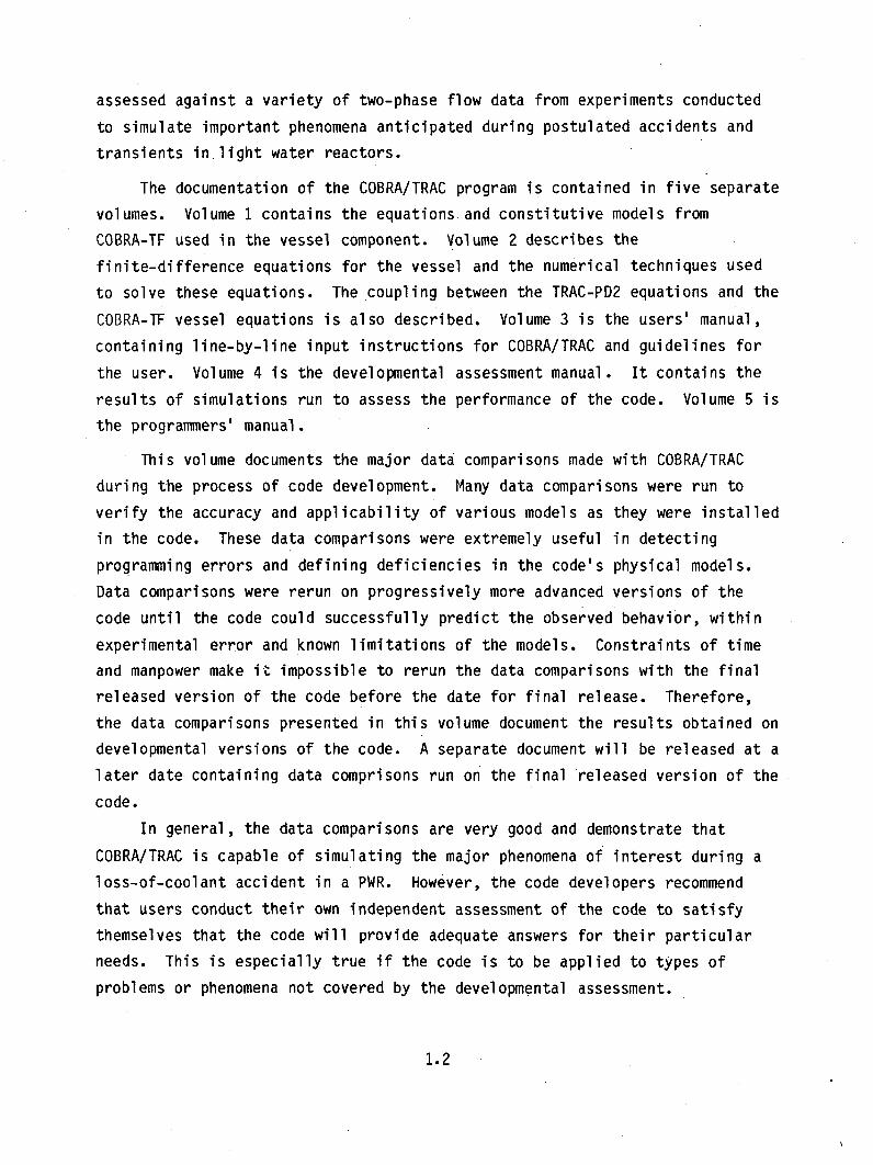
The documentation of the COBRA/TRAC program is contained in five separate
volumes. Volume 1 contains the equations and constitutive models from
COBRA-TF used in the vessel component. Volume 2 describes the
finite-difference equations for the vessel and the numerical techniques used
to solve these equations. The coupling between the TRAC-PD2 equations and the
COBRA-TF vessel equations is also described. Volume 3 is the users' manual,
containing line-by-line input instructions for COBRA/TRAC and guidelines for
the user. Volume 4 is the developmental assessment manual. It contains the
results of simulations run to assess the performance of the code. Volume 5 is
the programmers' manual.
This volume documents the major data comparisons made with COBRA/TRAC
during the process of code development. Many data comparisons were run to
verify the accuracy and applicability of various models as they were installed
in the code. These data comparisons were extremely useful in detecting
programming errors and defining deficiencies in the code's physical models.
Data comparisons were rerun on progressively more advanced versions of the
code until the code could successfully predict the observed behavior, within
experimental error and known limitations of the models. Constraints of time
and manpower make it impossible to rerun the data comparisons with the final
released version of the code before the date for final release. Therefore,
the data comparisons presented in this volume document the results obtained on
developmental versions of the code. A separate document will be released at a
later date containing data comprisons run on the final released version of the
code.
In general, the data comparisons are very good and demonstrate that
COBRA/TRAC is capable of simulating the major phenomena of interest during a
loss-of-coolant accident in a PWR. However, the code developers recommend
that users conduct their own independent assessment of the code to satisfy
themselves that the code will provide adequate answers for their particular
needs. This is especially true if the code is to be applied to types of
problems or phenomena not covered by the developmental assessment.
1.2

2.0 DATA COMPARISONS PERFORMED WITH DEVELOPMENTAL VERSIONS OF COBRA/TRAC
This section discusses the data comparisons made during the development
of COBRA/TRAC. The great majority were run on later versions of the code,
notably cycles 8, 10 and 11 (the released version is cycle 13). (See
Appendix A for a description of code cycles.)
The developmental assessment simulations fall into three main categories:
- basic tests
- separate effects tests
- integral systems tests
These tests include a large variety of two-phase flow and heat transfer
phenomena important in reactor safety. The code has been compared with data
for the following phenomena:
countercurrent flow limiting (CCFL)
downcomer ECC bypass with condensation, hot wall and transient effects
top and bottom reflood
condensation
phase separation (lateral void drift)
CHF and post-CHF
subcooled boiling
natural circulation
nucleate boiling (axial void profile and two-phase AP)
uncoveri ng/recovery
upper head draining
system simulations
The basic tests performed include:
RPI phase distribution
University of Houston tube CCFL
Dartmouth tube CCFL
NWU orifice plate CCFL
Bennett CHF and post-CHF heat transfer
NWU condensation on a falling liquid film
2.1
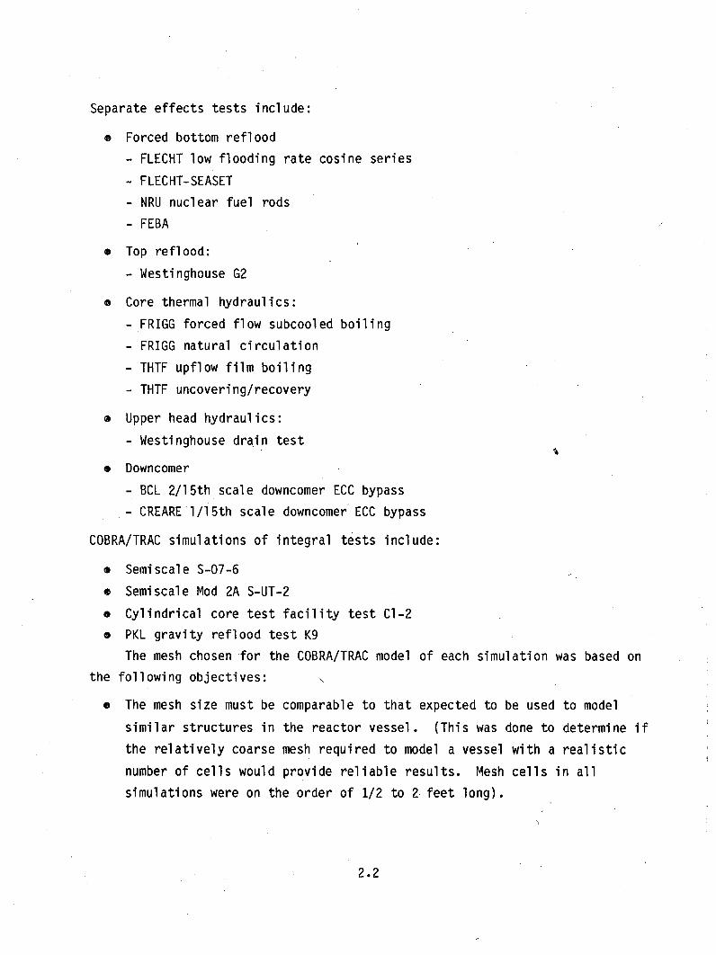
Separate effects tests include:
" Forced bottom reflood
- FLECHT low flooding rate cosine series
- FLECHT-SEASET
- NRU nuclear fuel rods
- FEBA
* Top reflood:
- Westinghouse G2
" Core thermal hydraulics:
- FRIGG forced flow subcooled boiling
- FRIGG natural circulation
- THTF upflow film boiling
- THTF uncovering/recovery
" Upper head hydraulics:
- Westinghouse drain test
" Downcomer
- BCL 2/15th scale downcomer ECC bypass
- CREARE 1/15th scale downcomer ECC bypass
COBRA/TRAC simulations of integral tests include:
* Semiscale S-07-6
" Semiscale Mod 2A S-UT-2
* Cylindrical core test facility test Cl-2
* PKL gravity reflood test K9
The mesh chosen for the COBRA/TRAC model of each simulation was based on
the following objectives:
* The mesh size must be comparable to that expected to be used to model
similar structures in the reactor vessel. (This was done to determine if
the relatively coarse mesh required to model a vessel with a realistic
number of cells would provide reliable results. Mesh cells in all
simulations were on the order of 1/2 to 2 feet long).
2.2
" A sufficient number of mesh cells must be used to model the physical
geometry of the experiment and to capture the dominant physical
phenomena. (In most simulations, a one-dimensional mesh was sufficient.)
" The number of mesh cells must be minimized to reduce computation costs as
much as possible while maintaining a sufficient degree of accuracy.
The selection of a mesh that satisfies these criteria requires the code
user to exercise his judgment. Experience and familiarity with the modeling
techniques used in COBRA/TRAC will be helpful, but the user may also have to
experiment with different meshes before selecting the most suitable one for a
given problem.
The meshes chosen for the simulations contained in this document are the
result of the experienced judgment of the code developers and early users.
They should be used as guidelines in setting up models for other
simulations. They should not be considered as perfect nor as an all-inclusive
list of possible meshes.
2.1 DARTMOUTH COUNTERCURRENT FLOW TUBE FLOODING EXPERIMENTS
Simulations were made of the Dartmouth College (Ref. 2) air-water
countercurrent flow flooding experiments in vertical tubes. There were three
main objectives in performing these simulations. First and foremost was to
evaluate the physical models for entrainment of drops from a falling liquid
film by the countercurrent vapor (or in this case, air) flow. Secondly, this
data provided a means to evaluate the models for interfacial shear between the
air and liquid film. Finally, this simulation provided experience in
determining the best mesh to model a liquid pool above a tube or orifice.
2.1.1 Description of Experiment
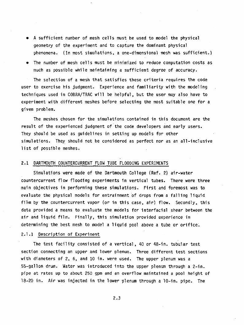
The test facility consisted of a vertical, 40 or 48-in. tubular test
section connecting an upper and lower plenum. Three different test sections
with diameters of 2, 6, and 10 in. were used. The upper plenum was a
55-gallon drum. Water was introduced into the upper plenum through a 2-in.
pipe at rates up to about 250 gpm and an overflow maintained a pool height of
18-20 in. Air was injected in the lower plenum through a 10-in, pipe. The
2.3
liquid penetration rate was determined by measuring the liquid accumulation
rate in the lower plenum. A schematic of the test section is shown in
Figure 2.1-1.
The experimental procedure was as follows:
" Airflow was set at a high enough value to stop all liquid penetration
into the flooding tube.
" The water supply was then turned on, and a liquid pool was allowed to
form in the upper plenum.
" Airflow was decreased, allowing water to penetrate the tube.
* Water accumulation in the lower plenum was measured.
* Airflow was checked for constancy.
2.1.2 COBRA/TRAC Model
In reactor safety applications, injected cooling water must penetrate
tubes or orifice plates against countercurrent steam flow. The accumulation
of water above tie plates results in the formation of a liquid pool. It is
therefore essential to model the flow in the liquid pool correctly to obtain
accurate inlet conditions for the flooding tube or orifice. The most
important aspects to model are the velocity and void fraction distributions in
the pool. When a high-velocity vapor enters a pool from a tube or orifice, it
can be expected that a high-velocity, high-void fraction region will exist in
the pool directly above the tube or orifice, while the fluid in the pool
surrounding the inlet tube or orifice remains at low velocity and low void
fraction. One might expect a two-phase jet consisting of vapor and water
drops at higher vapor velocities or water and vapor bubbles at lower vapor
velocities. Liquid in the two-phase jet above the inlet should be rising
while that surrounding the inlet may be falling.
The void and velocity distribution in the pool can be modeled by
two-fluid computer codes if a sufficiently small mesh is used to resolve the
gradients. However, this would require a very large number of mesh cells to
model the liquid pool in the upper plenum of a PWR, which has several vapor
jets entering the pool through orifices in the top nozzles of the fuel
assemblies.
2.4

UPPER PLENUM
AIR COMPRESSOR LOWER WATERPLENUM DRAINAGE
FIGURE 2.1-1. Experimental Setup for Flooding in Large Tubes
The optional subchannel formulation of the momentum equation and
channel-splitting capability available in COBRA/TRAC can be used to model the
pool with a reasonable number of nodes. This is done by modeling the pool in
each region of the upper plenum with two subchannels; one for the area
directly above the holes and the other for the area surrounding the holes.
The channel directly above the holes has the same flow area and hydraulic
diameter as the holes. This provides a two-region model of the pool, that has
been successfully used to predict CCFL in a variety of geometries.0
The test section was modeled with a single column 10 mesh cells high.
The bottom two mesh cells were used to model the collection of water in the
lower plenum. The upper plenum was modeled with two columns of mesh cells
(i.e., two channels). One channel was located directly above the test section
and had the same flow area and hydraulic diameter as the tube. The second
channel modeled the flow area in the remainder of the upper plenum. The
subchannel formulation of the momentum equation was used for the cross-flow
between these two channels. Air was modelled with steam at a suitable pressure
(-30 psi) to give a density equivalent to that of the air used in the
2.5

experiment. (This was done because only the equation of state for steam, not
air, is available in the code.) The steam was injected into the third mesh
cell of the lower plenum. Water was injected in the first cell of the upper
plenum. The overflow was modeled with a pressure boundary condition in the
fourth cell of the upper plenum, which provided the correct liquid head in the
pool. A node length of 6 in. was used in this simulation.
2.1.3 Discussion of Results
Experimental results were presented on plots of dimensionless gas flux,*1/2, 1j*/2,(1g )I, as a function of dimensionless liquid penetration flux, (J /
where for the ith phase:
1/2 (2.1)
EgD(pf - pg)]i12[gDg
where D is the diameter of the test section, j is the phase superficial
velocity, g is the acceleration of gravity and p is the density.
COBRA/TRAC predictions of the 2-in. tube experimental results are shown
in Figure 2.1-2. The comparison is quite reasonable. At high airflow rates,
film stability and entrainment in the test section or at the tube inlet
limited the rate at which liquid could penetrate to the lower plenum. At
lower airflow rates, liquid penetration was limited by the bubbly flow in the
pool above the test section inlet. COBRA/TRAC predictions of the 10-in, tube
experimental data are shown in Figure 2.1-3. The comparison is very
reasonable and the limiting behavAor was similar to that for the 2-in. test
section.
This simulation was run on cycle 8 of COBRA/TRAC. Significant deviations
in the prediction would be unlikely if the simulation were rerun on the final
code version. Some minor changes in the interpolation between the small and
large bubble flow regimes may affect the results as may the modification of
the unstable film friction factor.
2.6

lin10 o 2 IN. PIPE -
SINGLE SET OF MEASUREMENTS
* COBRA-TF PREDICTION~Ju°I
0.6c..J
* 0'
0.4%0 ý
Nl~0.2
0 . I I II I . . . .
0 0.2 0.4 0.6
* 1/2f
0.8 1.0
FIGURE 2.1-2. Liquid Penetration in 2-in. Tube
1.0
0.8
cmJ
0.6
0.4
0.2
o DATA 101N. PIPE
* COBRA-TF PREDICTION
• I II I I, I I I0
0 0.2 0.4 0.6 0.8 1.0
i*if
1/2
FIGURE 2.1-3. Liquid Penetration in 10-in. Tube
2.7
2.2 NORTHWESTERN UNIVERSITY ORIFICE PLATE FLOODING EXPERIMENT
Air-water countercurrent flow experiments in a vertical test section
containing an orifice plate were conducted at Northwestern University
(Ref. 3). The experiments studied the penetration of liquid through the holes
of the orifice plate against the upflow of air. This experiment was simulated
with COBRA/TRAC to assess the applicability of the nodalization developed for
a liquid pool above a tube (described in Section 2.1) to the pool above an
orifice plate. This simulation demonstrated the capability to predict the
correct liquid penetration through the orifice plate at various air (vapor)
velocities.
2.2.1 Description of Experiment
The experimental test section consisted of a vertical, rectangular box
made of brass with a Lexan front and back to allow observation of the flow
during the experiment. An orifice plate divided the test section into an
upper and lower section. Air was injected into the lower section at a
specified rate while water was injected into the upper section. The water was
injected through a vertical tube that was sealed off on the end and had
several small holes drilled around its perimeter to minimize the effects of
momentum of the injected liquid. Orifice plates with various hole sizes and
numbers of holes were investigated. An overflow pipe was connected to the
upper plenum to maintain a constant pool height. An air outlet pipe was
connected above that. A schematic of the test facility is shown in
Figure 2.2-1.
Experiments were performed for different orifice plates, liquid injection
nozzle elevations, and water flow rates. The experimental procedure was as
follows:
* Water flow was initiated in the upper plenum.
" Air flow was adjusted to the desired rate.
" The liquid penetration rate was measured.
The procedure was repeated with higher air flow rates.
2.8

WATER FLOW
AIRPRESSURE
OVERFLOWPRESSURE
ORIFICE PLATE
00000 ,AIRFLOW
0000000000
15 HOLE
FIGURE 2.2-1. COBRA/TRAC Model of Northwestern University CCFL ExperimentalFacility
2.2.2 COBRA/TRAC Model Description
A test containing an orifice plate with fifteen 10.5 mm holes arranged in
a 3x5 rectangular array was selected for this simulation. The liquid pool
above the orifice plate was modeled with two columns of mesh cells using a
subchannel approximation for the lateral flow between the two. This was done
to model the void and velocity profiles in the pool as described in
Section 2.1. The first channel had a flow area equal to the total area of the
15 holes and a hydraulic diameter equal to the diameter of a single hole. The
second channel modeled the area surrounding the holes. A node length of 5 in.
was used.
Two channels were used below the orifice plate. The lower one served as
a liquid collection volume, and the top one modeled the region below the
orifice plate into which air was injected. Liquid was injected into the fifth
axial node in the upper plenum. Since the liqiud was injected from the side,
it was assumed for the COBRA/TRAC model that the injected fluid had no
vertical component of momentum.
2.9

2.2.3 Discussion of Results
Experimental results were presented on plots of dimensionless gas flux,g*I/2 *I/2whrH as a function of dimensionless liquid penetration flux, H* 1
for the ith phase
H Pi 1/2 iHi = (2.2)
1 [gW8 (pt - Pg)]I/Z
where W8 is a characteristic dimension that is an interpolation between DH
used in J scaling and the wave length of the Taylor instability,
{/[g(Pf - P )]}I/2, used in k* scaling.
The following definitions hold for the above equation:
W = DHI-*) [a/g (Pf-P )]*/2 (2.3)
= tanh [(K DH) (Ah)/AT)] (2.4)
DH = hydraulic diameter of the hole in the perforated plateH*
= interpolation function between J and k scaling
Ah = total area of holes in perforated plate
AT = total area of test cross section
K = wave number (plate thickness/2)
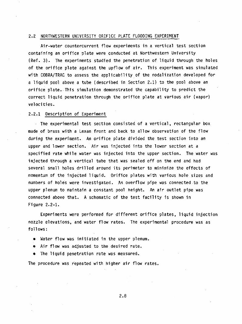
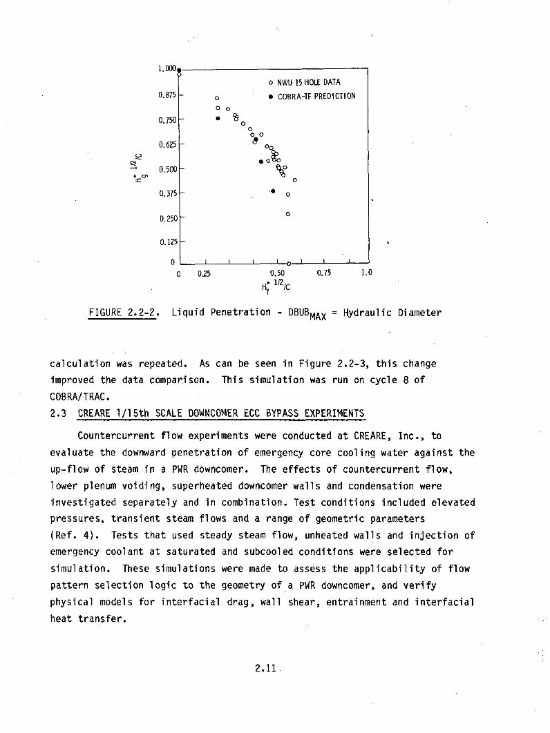
COBRA/TRAC data predictions are shown in Figure 2.2-2. The predictions
are quite reasonable, with bubbly flow in the pool limiting liquid penetration
at all vapor velocities. At lower vapor velocities less liquid penetration
was predicted than was measured experimentally.
The bubble size is limited in the calculation to the hydraulic diameter
of the holes. With holes located so close together it is probable that
bubbles coalesced and that larger bubble diameters are possible. The limit on
bubble sizes was arbitrarily set to twice the hole diameter and the
2.10
S 0.500 -
0
0.375 - 0
0.250 0
0.125
0 00 025 0.50 0.75 1.0
H 112/CHf
FIGURE 2.2-2. Liquid Penetration - DBUBMAX = Hydraulic Diameter
calculation was repeated. As can be seen in Figure 2.2-3, this change
improved the data comparison. This simulation was run on cycle 8 of
COBRA/TRAC.
2.3 CREARE 1/15th SCALE DOWNCOMER ECC BYPASS EXPERIMENTS
Countercurrent flow experiments were conducted at CREARE, Inc., to
evaluate the downward penetration of emergency core cooling water against the
up-flow of steam in a PWR downcomer. The effects of countercurrent flow,
lower plenum voiding, superheated downcomer walls and condensation were
investigated separately and in combination. Test conditions included elevated
pressures, transient steam flows and a range of geometric parameters
(Ref. 4). Tests that used steady steam flow, unheated walls and injection of
emergency coolant at saturated and subcooled conditions were selected for
simulation. These simulations were made to assess the applicability of flow
pattern selection logic to the geometry of a PWR downcomer, and verify
physical models for interfacial drag, wall shear, entrainment and interfacial
heat transfer.
2.11.

1.000
o NWU 15 HOLE DATA
0.875 - 0 COBRA-TF PREDICTION0 0O
0.750 -00 0
0.625 o
0.500
0.375
0.250 0
0.125
0 I I I o I I I
0 0.25 0.50 0.75 1.0
H* 1/2/CHf
FIGURE 2.2-3. Liquid Penetration - DBUBMAX= 2* (hydraulic diameter)
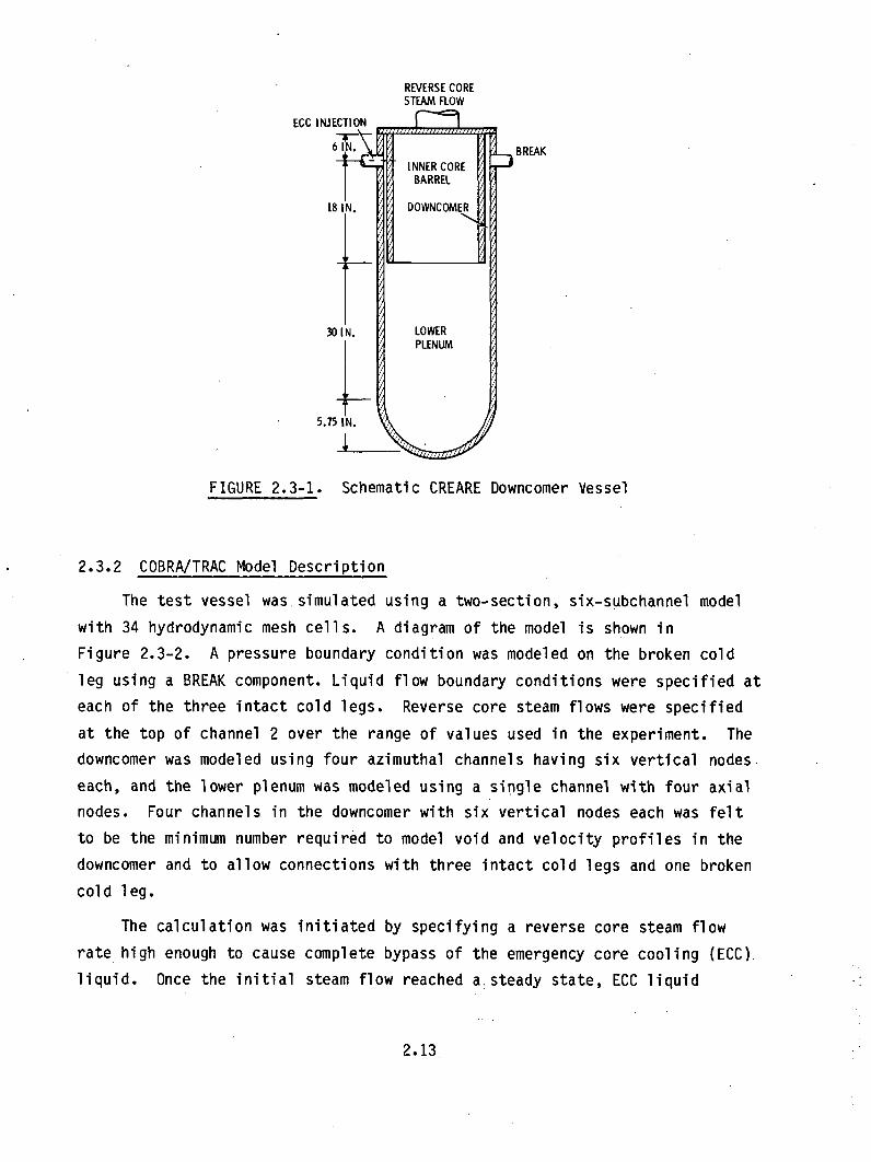
2.3.1 Description of Experiment
The test apparatus consisted of a cylindrical vessel containing a
1/15-scale PWR downcomer and an extended lower plenum. Figure 2.3-1 shows a
diagram of the test section. The downcomer gap and circumference were 0.5 in.
and 34.6 in., respectively. Three intact cold legs and one broken cold leg
were connected to the top of the downcomer. Emergency core cooling water was
injected into each of the three intact cold legs. The broken cold leg was
connected to a separator. Steam was injected in the top of the vessel on the
inside of the core barrel to simulate reverse core steam flow.
Tests were run by first injecting a constant steam flow rate through the
vessel, purging the vessel of air, and then injecting water at a constant rate
through the intact cold legs into the downcomer. The flow was then allowed to
achieve dynamic equilibrium, and the liquid penetration rate into the lower
plenum was measured. This procedure was repeated at different steam flow
rates for each liquid injection rate and temperature, covering the range from
complete bypass of the injected liquid out the broken cold leg to complete
penetration of the liquid into the lower plenum.
2.12
REVERSE CORESTEAM FLOW
ECC INJECTION• . BREAK6 IN. INNER CORE BRA
BARREL
18 IN. DOWNCOMER
30 I N. LOWER
PLENUM
5.75 IN.
FIGURE 2.3-1. Schematic CREARE Downcomer Vessel
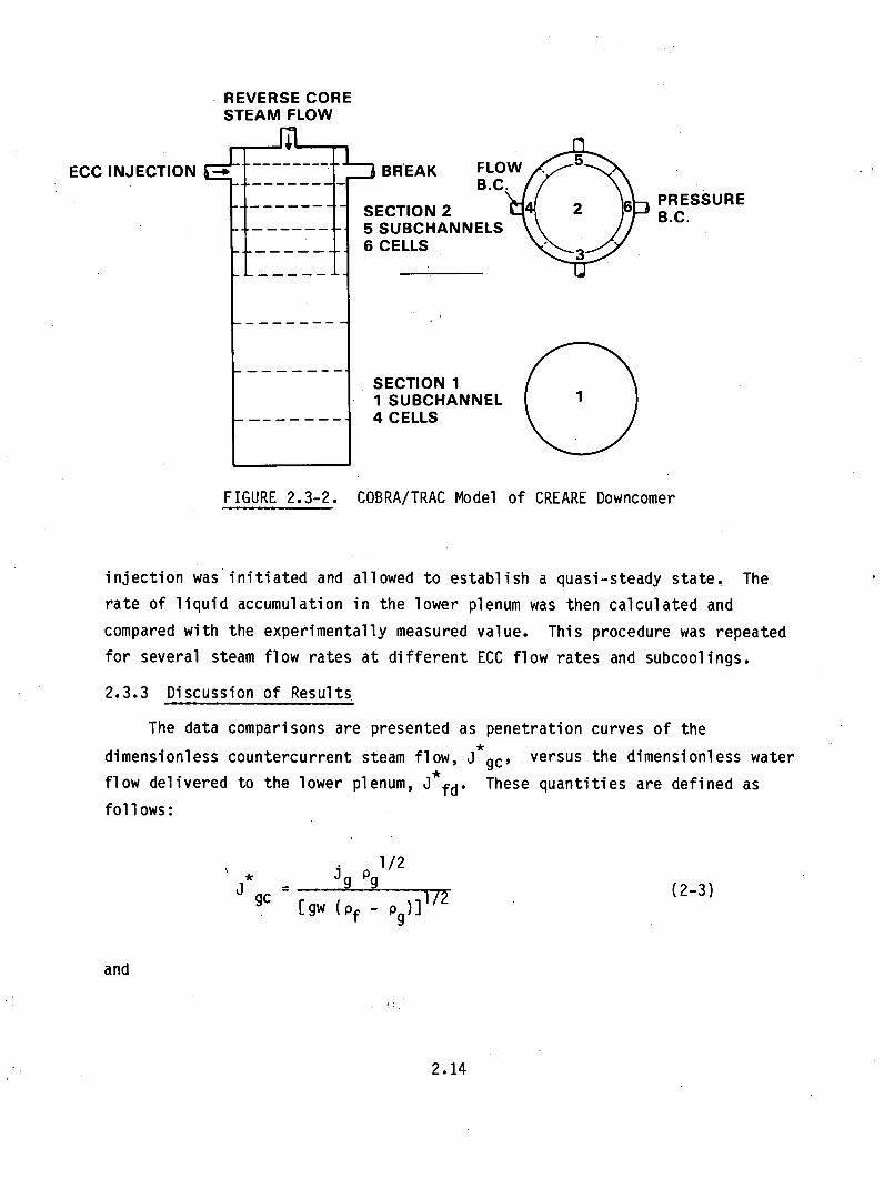
2.3.2 COBRA/TRAC Model Description
The test vessel was simulated using a two-section, six-subchannel model
with 34 hydrodynamic mesh cells. A diagram of the model is shown in
Figure 2.3-2. A pressure boundary condition was modeled on the broken cold
leg using a BREAK component. Liquid flow boundary conditions were specified at
each of the three intact cold legs. Reverse core steam flows were specified
at the top of channel 2 over the range of values used in the experiment. The
downcomer was modeled using four azimuthal channels having six vertical nodes
each, and the lower plenum was modeled using a single channel with four axial
nodes. Four channels in the downcomer with six vertical nodes each was felt
to be the minimum number required to model void and velocity profiles in the
downcomer and to allow connections with three intact cold legs and one broken
cold leg.
The calculation was initiated by specifying a reverse core steam flow
rate high enough to cause complete bypass of the emergency core cooling (ECC)
liquid. Once the initial steam flow reached a steady state, ECC liquid
2.13
ECC INJECTION '
REVERSE COISTEAM FLOW
7 BREAKFLOWB.C.
4-4 SECTION 25 SUBCHANNELS6 CELLS
SECTION 11 SUBCHANNEL4 CELLS
PRESSUREB.C.
FIGURE 2.3-2. COBRA/TRAC Model of CREARE Downcomer
injection was initiated and allowed to establish a quasi-steady state. The
rate of liquid accumulation in the lower plenum was then calculated and
compared with the experimentally measured value. This procedure was repeated
for several steam flow rates at different ECC flow rates and subcoolings.
2.3.3 Discussion of Results
The data comparisons are presented as penetration curves of the
dimensionless countercurrent steam flow, J *gc, versus the dimensionless water
flow delivered to the lower plenum, J*fd" These quantities are defined as
fol lows:
,c = pg1/2
[gw (Pf - Pg)]I(2-3)
and
2.14

if jf 1f/2* fp (2-4)
Ifd [gw (Pf 9)]1/2(-
where jg and jf are the vapor and liquid volumetric fluxes at the base of the
downcomer, pg and pf are the vapor and liquid densities, and w is the downcomer
ci rcumference.
Figures 2.3-3 and 2.3-4 show the penetration curves for ECC injection of
saturated water at injection rates of 30 and 120 gpm, respectively. At 30
gpm, the experimental data indicate that complete bypass occurs for
dimensionless steam flows greater than 0.18, partial penetration between 0.18
and 0.04, and complete penetration below 0.04. COBRA/TRAC slightly
overpredicts the penetration rate; however, this data comparison is
acceptable. The data comparison for the 120 gpm penetration curve is good.
Liquid begins to penetrate the downcomer at J*fd = 0.18 with COBRA/TRAC
slightly underpredicting the filling rate until a transition occurs at
J*fd = 0.11. This occurred as the liquid reached the bottom of the downcomer
on the side opposite the break, allowing a sudden increase in liquid
penetration.
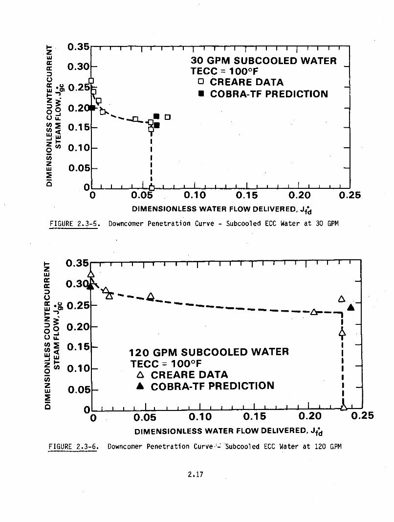
These saturated ECC penetration curves assessed the code's ability to
predict the momentum transfer in the downcomer. The subcooled ECC injection
tests assessed the condensation heat transfer in the downcomer. Figures 2.3-5
and 2.3-6 show the penetration curves when liquid at 100°F(~1150 F subcooled)
is injected at 30 and 120 gpm. At both flow rates COBRA/TRAC predicts the
transition from complete bypass to complete penetration very well. Partial
penetration at high ECC subcoolings is actually a time average of periods of
complete bypass and periods of complete penetration (periodic downcomer
filling and dumping). These simulations were run with cycle 8.
2.4 BATTELLE COLUMBUS 2/15th SCALE DOWNCOMER TRANSIENT ECC BYPASS EXPERIMENT
Two transient Battelle Columbus downcomer tests were simulated. These
experiments were part of the Steam-Water Mixing and System Hydrodynamics
program conducted at Battelle in Columbus, Ohio (Ref. 5,6,7). The purpose was
2.15

0.30
0.25
~ ' 0.2oO.O 0.1
LU
ZoU• 0.100jý
30 GPM SATURATED WATER
rICREARE DATAACOBRA-TF PREDICTION
A
A
A
A0.05
00 0.02 0.04
DIMENSIONLESS WATER0.06
FLOW DELIVERED, Jfd*0.08
FIGURE 2.3-3. Downcomer Penetration Curve - Saturated ECC Water at 30 GPM
-j
U-
fI-
Ln
V-)
C-j
L/,
cm
0.4
0.3
120 G PM SATURATED WATER
A CREARE DATA
A COBRA-TF PREDICTION
AAA
I A II II AlI
0.2
0.1
U
0.05 0.10 0.15 0.20 0.25
DIMENSIONLESS WATER FLOW DELIVERED JfI'd
FIGURE 2.3-4. Downcomer Peneltration Curve - Saturated ECC Water at 120 GPM
2.16
Ui
L),,=
I,.z0
C.J
0o
z
Ui
0.35
0.30 -
0.2 5
'I i II I IIII I I I I j II ,
30 GPM SUBCOOLED WATERTECC = 100OF
o CREARE DATA* COBRA-TF PREDICTION
0-lU-
wj
0.20no
0.15-
0.10 -IIIII0.05
0 0.05I I . , , I I I a a I I I I I I
0.10 0.15 0.20 0.25DIMENSIONLESS WATER FLOW DELIVERED, Jf*
FIGURE 2.3-5. Downcomer Penetration Curve - Subcooled ECC Water at 30 GPM
I-
z0
I-z0
z0j
0.35 ,,
0 .3 (*%
0.25-
0.20
I I 1 1 1I 1 1 1i f l - 1 - - -I-i--1 I
0-IU.
wI-Co
-~A
0.15k
0.101-
120 GPM SUBCOOLED WATERTECC = 100OFA CREARE DATAA COBRA-TF PREDICTION
IIIIIII0.05 I
I
n I II
0.250 0.05 0.10 0.15 0.20DIMENSIONLESS WATER FLOW DELIVERED, Jfd
FIGURE 2.3-6. Downcomer Penetration Curve-.: 'Subcooled ECC Water at 120 GPM
2.17

to study the interactions between steam and the ECC fluid within the primary
system. Of particular interest here are the tests concerned with the ECC
bypass behavior in the downcomer annulus. These calculations assessed
COBRA/TRAC's ability to predict the combined effects of ramped reverse core
steam flow, subcooled emergency core cooling (ECC) water, and hot walls on the
ECC bypass behavior during countercurrent flow in a downcomer.
2.4.1 Description of Experiment
The test vessel was a 2/15th-scale PWR downcomer with an extended lower
plenum. Four cold legs were arranged in a 600 to 120' orientation with a hot
leg plug (7.84 in. O.D.) located in the center of the two 1200 arcs. Each of
the three intact cold legs modeled the loop piping from the steam generator
exit to the vessel and included the pump suction piping and a simulated
pump. The broken cold leg discharged into a pressure controlled containment
tank. The principle dimensions of the vessel are shown in Figure 2.4-1. The
downcomer was 41 in. high, had a circumference of 72.6 in. and a downcomer gap
,width of 1.23 in.
Steam was injected in the top of the vessel at a prescribed rate. It
flowed into the lower plenum, up the downcomer and out the broken leg to the
containment vessel. ECC water was injected at a constant rate in each of the
intact loops. Depending on the instantaneous steam and ECC flow rate, the
subcooling of the ECC water and the initial temperature of the downcomer
walls, liquid would either bypass the downcomer and be carried by the steam
out the break or penetrate the downcomer and flow into the lower plenum.
Because the tests all had decreasing steam ramps, the behavior was initially
complete bypass, then as the steam flow rate decreased, partial bypass and
finally complete penetration to the lower plenum.
2.18

CORESTEAM
ECC INJECTION
BREAK
41. 0"
S21. 89" - -
• 24. 35 ..
40.25"
FIGURE 2.4-1. Diagram of Battelle Columbus 2/15-th Scale Downcomer Vessel
The test procedure used in the ramped steam flow rate, hot wall tests was
as follows:
" Using steam, the vessel was heated to the required wall temperature.
* The ECC water injection rate and initial reverse core steam flow rate
were established by routing these flows to the ECC supply tank and
containment vessel, respectively.
" Simultaneously, the steam and ECC flows were switched to the vessel and
the decreasing steam ramp was initiated.
Pressures, temperatures and liquid levels were recorded during the tests.
2.4.2 COBRA/TRAC Model Description
The COBRA/TRAC vessel nodalization to model the BCL downcomer test is
shown in Figure 2.4-2. It consists of 57 hydrodynamic cells in 9 channels and
2 sections. Section 1 models the lower plenum using 1 channel and 4 axial
levels spaced 10 in. apart. Channel 2 models the region beneath the downcomer
and connects to channels 4 through 9 above. Section 2 models the downcomer
2.19

CORESTEAM FILL
ECC
BREAK INJECTION
fB REA K FILL
-SECTION 296
7 SUBCHANNELS
7 LEVELS
8FILL
SECTION 1
2 SUBCHANNELS 2
4 LEVELS
FIGURE 2.4-2. COBRA/TRAC Model of BCL Downcomer
and inner core barrel using 7 axial cells, each 6 in. high. The reverse core
steam flow rate versus time was specified at the top of channel 3 using a mass
flow rate boundary condition. ECC injection rates in the sixth level of
channels 5, 6 and 8 were also specified using boundary conditions. The
pressure boundary condition at the broken cold leg was modeled using PIPE and
BREAK components. The hot leg plugs were simulated by applying zero flow rate
boundary conditions at each face of the sixth hydrodynamic cell in channels 4
and 7. Six channels were used in the downcomer to model velocity and void
profiles, the four cold leg connections and the hot leg plugs.
The physical structure of the test section was modeled with 12 rods, each
representing a fraction of the downcomer circumference seen by the channels.
The conduction heat transfer model was used to calculate the effects of stored
energy in the vessel and downcomer walls.
Two tests, 404 and 501, were simulated. Table 2.1 summarizes the test
conditions. The ramps used on the reverse core steam flow rate (Ref. 7) are
given in Table 2.2. Test 501 was run at a higher pressure and initial wall
2.20
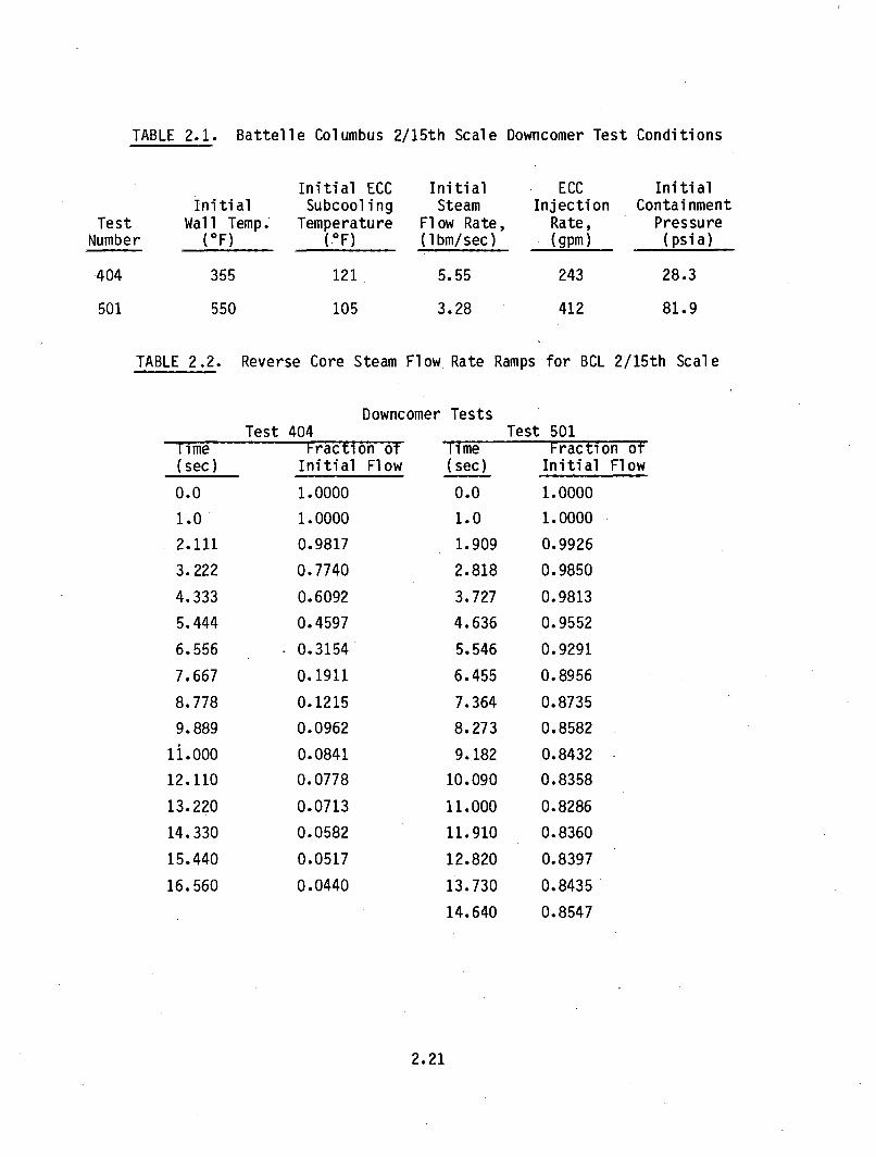
TABLE 2.1. Battelle Columbus 2/15th Scale Downcomer Test Conditions
TestNumber
404
501
InitialWall Temp.'
(OF)
355
550
Initial ECCSubcooling
Temperature(OF)
121
105
InitialSteam
Flow Rate,(lbm/sec)
5.55
3.28
ECCInjection
Rate,(gpm)
243
412
InitialContainment
Pressure(psia)
28.3
81.9
TABLE 2.2. Reverse Core Steam Flow Rate Ramps for BCL 2/15th Scale
Downcomer TestsTest 404
I ime(sec)
0.0
1.0
2.111
3.222
4.333
5.444
6.556
7.667
8.778
9.889
1i.000
12.110
13. 220
14. 330
15.440
16. 560
Mrcf-ion OTInitial Flow
1.0000
1.0000
0.9817
0.7740
0.6092
0.4597
0.3154
0.1911
0.1215
0.0962
0.0841
0.0778
0.0713
0.0582
0.0517
0.0440
time(sec)
0.0
1.0
1.909
2.818
3.727
4.636
5.546
6.455
7.364
8.273
9.182
10.090
11.000
11.910
12.820
13.730
14.640
Test 501Frraction o-
Initial Flow
1.i0000
1.0000
0.9926
0.9850
0.9813
0.9552
0.9291
0.8956
0.8735
0.8582
0.8432
0.8358
0.8286
0.8360
0.8397
0.8435
0.8547
2.21

temperature than 404. It also had a larger ECC injection rate, and a smaller
steam flow rate. Therefore, it should allow a faster filling rate than
test 404.
2.4.3 Discussion of Results
Figures 2.4-3 and 2.4-4 show the lower plenum liquid volume versus time
for the ramped steam hot wall tests 404 and 501. (ECC injection began at 1
sec.) The data comparison is good. COBRA/TRAC predicted the initial delay
time to within 1 sec. The filling rate for test 404 was in excellent
agreement. A slightly higher filling rate occurred in test 501, because the
containment pressure used in COBRA/TRAC was too high. During periods of
condensation, the containment pressure was greater than the lower plenum
pressure and reverse break flow was predicted.
The condensation led to flow oscillations in the downcomer. During
periods of condensation the pressure in the lower plenum decreased and the
rate of liquid delivery increased. This is shown in Figure 2.4-5 a plot of
the lower plenum pressure, and Figure 2.4-6, a graph of the net condensation
rate in the vessel. For example, the condensation rate at 15 sec is high
(nearly 6.0 Ibm/sec), while the pressure is low (about 18 psia). This caused
the lower plenum filling rate to increase as shown in Figure 2.4-3. As the
condensation increased and decreased, the rate of liquid delivery to the lower
plenum oscillated.
Most of the delivery occurred on the side of the downcomer opposite the
broken cold leg. Starting from the bottom of the downcomer and moving up, the
flow pattern was: film flow, then inverted pool where the liquid fraction
typically increased from 0.05 to 0.8, and finally bubbly flow. Generally, the
farther around the downcomer circumference from the break, the lower the
transition to inverted pool occurred. As a result, the film to bubble
interface was tilted with the lower side opposite the broken cold leg.
COBRA/TRAC's predictions of the lower plenum filling rate agrees well
with the data. This implies that the physical models for phase interfacial
drag and heat transfer in the film, inverted pool and bubbly flow regimes are
properly representing the ECC bypass behavior in the downcomer. This
simulation was run on cycle 8 of COBRA/TRAC.
2.22
BCL LOWER PLENUM LIQUID VOLUME
12
10
SD
11SD
>6
:2 4
0:
3
*-~ 2
4 9 12 16 20
TiME (SECONDS)
Lower Plenum Liquid Volume vs. Time.for Test 404FIGURE 2.4-3.
BCL LOWER PLENUM LIQUID VOLUME
12
10
SD
8 9 12 16 20
TIME (SECONDS)
FIGURE 2.4-4. Lower Plenum Liquid Volume vs. Time for Test 501
2.23

BCL LOWER PLENUM PRESSURE
45
40
35
25
a
20
; 5
1'? 20TIME (SECONDS)
FIGURE 2.4-5. Lower Plenum Pressure vs. Time for Test 404
BCL CONDENSATION RATE VS. TIME
0.0
-3 6.5M
4.5
3.0
1.5
8 12
TIME (SECONDS)
16 20
FIGURE 2.4-6. Net Condensation Rate in the Vessel vs. Time for Test 404
2.24

2.5 FEBA FORCED BOTTOM REFLOOD EXPERIMENT
Forced flow bottom reflood experiments were performed in the Flooding
Experiments in Blocked Arrays (FEBA) test assembly in Karlsruhe, West Germany
(Ref. 8,9). The purpose of these experiments was to determine the effects of
grid spacers and flow blockages on reflood heat transfer. This was done by
performing a series of tests with different grid spacer and blockage
configurations. These included tests with normal grid spacers, tests with a
single grid spacer removed, and tests with sleeve blockages attached to heater
rods.
The test with normal grid spacers and no blockage was simulated with
COBRA/TRAC to assess the models used for reflood heat transfer and reflood
hydrodynamics.
2.5.1 Description of Experiment
The FEBA test facility, shown schematically in Figure 2.5-1, was
originally designed to simulate idealized reflood conditions in a German PWR
core with constant forced bottom reflood, system pressure and test section
geometry. The experimental test loop consisted of a lower plenum, a test
section with a 5x5 electrically heated rod bundle, an upper plenum, buffer
tank and associated piping.
During test operations, coolant was pumped from a storage tank into the
lower plenum of the test assembly. The water was regulated at a prescribed
level in the lower plenum and the heater rod and housing were heated to the
prescribed initial temperatures. Reflood water injection was then
initiated. Water entering the test section generated vapor as a result of
heat transfer from the heated rods. Steam and entrained water droplets were
transported upward through the test section and impinged on a steam/water
separator in the upper plenum. The separated water droplets were moved away
from the top o1 the heated length, reducing the amount of water fallback into
the test section. The steam flowed through the steam/water separator and into
a steam buffer tank. The buffer tank regulated the system pressure and exit
steam temperature. A square test section housing enclosed the test section
and connected the lower plenum to the upper pl~enum. The housing was insulated
to reduce heat losses to the environment.
2.25
BUFFERPRESSURE REGULATOR
UPPER PLENUM
STEAM SEPARATOR
WATERCOLLECTION
TAN K
TEST SECTIONTEST SECTION
- HOUSING
TEST RODS
LOWER PLENUM
WATER TANK
FIGURE 2.5-1. Schematic of FEBA Test Facility
2.26

The test section consisted of a 5x5 square array of electrical heater
rods. A cross-sectional view of the test section and one represe'ntative
heater rod are shown in Figure 2.5-2. The test section wall thickness was
6.5 mm. The rod pitch was 14.3 mm. The rod outside cladding diameter was
10.75 mm with a diametral clad thickness of 2.1 mm. The outside diameter of
the heater element was 8.55 mm. The upper ends of the heater rods were bolted
to the top of the test assembly while the lower ends were allowed to hang
free, permitting axial movement. Horizontal movement and/or bowing of the
rods was restricted by seven typical KWU-PWR grid spacers every 545 mm and
centered on the test section midplane.
The electrical heater rods were constructed of spiral-wound heating
elements embedded in magnesium oxide insulators. The cosine power profile of
nuclear fuel was approximated by a seven-step power profile. The length of
each power step and the peak-to-average power factors are shown in
Figure 2.5-3.
The test assembly was initially heated by radiation from the heater rods
for about 2 hours prior to reflood. During this heat-up phase the heater rods
were at a low power level and surrounded by stagnant steam. These test
conditions were maintained until the desired peak cladding temperatures were
reached.
Reflood was initiated after the cladding temperatures reached the
required initial temperature. Water was injected into the lower plenum with a
constant flow rate of 3.5 cm/sec, an inlet temperature of 40°C, and at a
pressure of 4 bars. When the rising water reached the lower end of the heated
length, the rod power was increased to the ANS + 20% decay heat level
corresponding to 40 seconds after scram. The power was then decreased
according to the ANS +20% curve during the remainder of the test. The
temporal power decay curve used for test run 216, normalized to Po, where Po
was the peak power at time zero is shown in Figure 2.5-4. The initial test
parameters for test 216 have been tabulated in Table 2.3.
2.27

HATE RD TEST HOUSINGHEATER RODS TEST HOUSING~X \NXNNXX~~3NNNNNXNN\NN\NNN.~\N\N\N
CLADDING (NICR 80/20) K O(ooo000000000000000000HEATING ELEMENT (NICR
80/20 SPIRAL WOUND
FIGURE 2.5-2. Cross Section of FEBARepresentative Heater
Test Section 5x5 Bundle andRod
75
375-
775-
1375 -
E •
2022•5
2675 -
3275
3675
39754114
2025mm
FIGURE 2.5-3. Axial Power Profile andSection
Grid Spacer Locations for FEBA Test
2.28

0.'055
0.050
0.045
PtPo 0.040
0.035
0.030
0.025
ANS + 20 POWER DECAY CURVE
40 sec. AFTER SCRAM
- ANS + 20 VALUES
- EXTRAPOLATED VALUES
s/
J III IiI I I I
0 100 200 300 400 500 600 700
TIME
FIGURE 2.5-4. Power Decay Curve for FEBA Test Run 216
TABLE 2.3. Boundary Conditions for FEBA Test 216
Initial peak rod temperature
Peak rod power
Constant flow rate
Inlet coolant temperature
System pressure
8000C
0.8 kW/ft
3.5 cm/sec400C
4 bars
2.5.2 COBRA/TRAC Model Description
The FEBA test facility was modeled with three components: a one-
dimensional vessel component with mass injection at the bottom boundary; a
PIPE component connected to the top of the vessel; and a BREAK component
connected to the pipe. The COBRA/TRAC nodalization schematic is shown in
Figure 2.5-5. The vessel component modeled the lower plenum, test section and
upper plenum. The total fluid flow area (38.9 cm2 ) was modeled using four
channels; one channel for the lower plenum and three for the heated length and
2.29
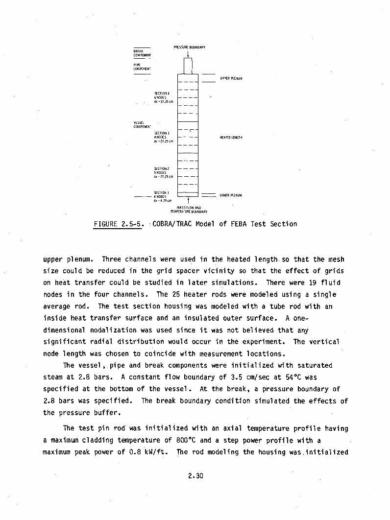
PRESSURE BOUNDiBREAKCOMPONENT
PI PECOMPONENT
SECTION 46 NODE S --dx -27.25cm
VESSELCOMPONENT
SECTION34 NODES -dx - 27.25 cm
SECTIONO - -5 NODESdx-27.25c- cm
SECTION I-- _ 4 NODES
dx - 4.25 cm T
MASS hLOW AN[TEMPERATURE BOUNI
FIGURE 2.5-5. "COBRA/TRAC M,
UPPER PLENUM
HEATED LENGTH
LOWER PLENUM
DARY
odel of FEBA Test Section
upper plenum. Three channels were used in the heated length. so that the mesh
size could be reduced in the grid spacer vicinity so that the effect of grids
on heat transfer could be studied in later simulations. There were 19 fluid
nodes in the four channels. The 25 heater rods were modeled using a single
average rod. The test section housing was modeled with a tube rod with an
inside heat transfer surface and an insulated outer surface. A one-
dimensional nodalization was used since it was not believed that any
significant radial distribution would occur in the experiment. The vertical
node length was chosen to coincide with measurement locations.
The vessel, pipe and break components were initialized with saturated
steam at 2.8 bars. A constant flow boundary of 3.5 cm/sec at 540C was
specified at the bottom of the vessel. At the break, a pressure boundary of
2.8 bars was specified. The break boundary condition simulated the effects of
the pressure buffer.
The test pin rod was initialized with an axial temperature profile having
a maximum cladding temperature of 800 0 C and a step power profile with a
maximum peak power of 0.8 kW/ft. The rod modeling the housing wasinitialized
2.30
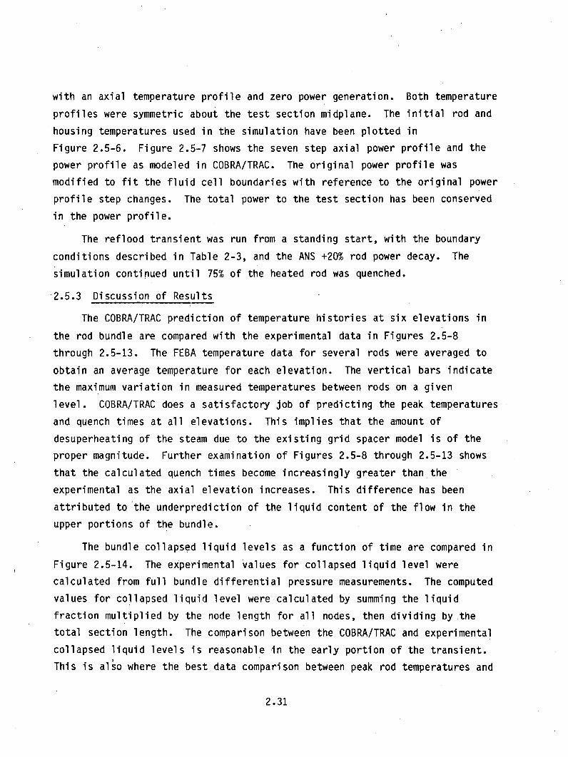
with an axial temperature profile and zero power generation. Both temperature
profiles were symmetric about the test section midplane. The initial rod and
housing temperatures used in the simulation have been plotted in
Figure 2.5-6. Figure 2.5-7 shows the seven step axial power profile and the
power profile as modeled in COBRA/TRAC. The original power profile was
modified to fit the fluid cell boundaries with reference to the original power
profile step changes. The total power to the test section has been conserved
in the power profile.
The reflood transient was run from a standing start, with the boundary
conditions described in Table 2-3, and the ANS +20% rod power decay. The
simulation continued until 75% of the heated rod was quenched.
2.5.3 Discussion of Results
The COBRA/TRAC prediction of temperature histories at six elevations in
the rod bundle are compared with the experimental data in Figures 2.5-8
through 2.5-13. The FEBA temperature data for several rods were averaged to
obtain an average temperature for each elevation. The vertical bars indicate
the maximum variation in measured temperatures between rods on a given
level. COBRA/TRAC does a satisfactory job of predicting the peak temperatures
and quench times at all elevations. This implies that the amount of
desuperheating of the steam due to the existing grid spacer model is of the
proper magnitude. Further examination of Figures 2.5-8 through 2.5-13 shows
that the calculated quench times become increasingly greater than the
experimental as the axial elevation increases. This difference has been
attributed to the underprediction of the liquid content of the flow in the
upper portions of the bundle.
The bundle collapsed liquid levels as a function of time are compared in
Figure 2.5-14. The experimental values for collapsed liquid level were
calculated from full bundle differential pressure measurements. The computed
values for collapsed liquid level were calculated by summing the liquid
fraction multiplied by the node length for all nodes, then dividing by the
total section length. The comparison between the COBRA/TRAC and experimental
collapsed liquid levels is reasonable in the early portion of the transient.
This is also where the best data comparison between peak rod temperatures and
2.31

400
W / • AMEASURED DATA PTS. FROM FEBA DATA\O EXTRAPOLATE DATA (BEST ESTIMATE)
//
200
HEATED LENGTH b(127.5--*4027.5 mm)
0 I I0000 2000 . 3000 4000 5000
DI STANCE FROM BOTTOM OF TEST SECTION (mm)
FIGURE 2.5-6. COBRA/TRAC Initial Rod Temperatures vs. Axial Position
AXIAL FLUID NO0(S ORIGINAL P707 R PROFILE COBRA-IF P77 VER PROFILE
E.NO OF 22MULATID LENGTH
2m0.0[ - .27--Z2.5 RB 0.426
S277.5- o. .n
N O 0.7 272. 5 mm 0.887
SC6227 24 545R m42,0
H4EATED LNGYH172.5772 27
1500 207.571,175
252 222.5 R 0.27
0 D8
542- 272.5 R. I.n72
35 4 "0.6 157 0.65
o 2.5 0.0 0.5 1.0
AXI&1 NODE 7W . P•I2 m272
FIGURE 2.5-7. Test Section Axial Power Profile and COBRA/TRAC Model of the
Axial Power Profile
2.32

1000
800
L.,0
I-2wU
600
FEBA TEST 216COBRA-TF @ 0.85mFEBA DATA @ 0.79m
0=- 0 %
w, I
-IIIII
LL0
1832
1652
1472
1292
1112
932
752
572
392
212
000
0
wi
Ui-
4i400
200
n
-100 0 100 200 300
TIME, SEC.
400 500 6(
FIGURE 2.5-8. COBRA/TRAC Predicted Rod Temperatures at 0.8m for FEBA Test 216
U.0
LU
I-
4U
1000
800
600
400
1832
1652
1472
1292
1112
932
752
572
392
212
0
U-0
Uj
4i
2 0 0
0-100
FIGURE 2.5-§.
0 100 200 300 400
TIME, SEC.
COBRA/TRAC Predicted Rod Temperatures
500 600
at 1.3m for FEBA Test 216
2.33

1000 1832
800
00
LU
LU
600
400
1652
1472
1292 O
w
1112 •
932
752 0.
572 U'
392
212
0
200
0--100 0 100 200 300
TIME,SEC.400 500 600
FIGURE 2.5-10. COBRA/TRAC Predicted Rod TemperaturesTest 216
at 1.9m for FEBA
C.0
LU
CL
LUI
1000
800
600
400
1832FEBA TEST 216
- COBRA-TF @ 2.35m -1652/" - FEBA DATA @ 2.44m 1472
-1292 u.0
-1112 L
932
- 752 LU
- 572 LU
-- 392
-.- 212
I I 00 100 200 300 400 500 600
TIME, SEC
200
0-100
FIGURE 2.5-11. COBRA/TRAC Predicted Rod TemperaturesTest 216
at 2.4m for FEBA
2.34

C.)0
LI-
1000
800
600
400
2 0 0 v
0-100
FIGURE 2.5-12.
1832FEBA TEST 216
-COBRA-TF @ 2.90m - 1652FEBA DATA @ 2.97m/-Z-•'•,,,,•_ 1472
.1292
0 ,1112
0 -\ 932w
1752
o-. I0 -.572
- 392I-- IC,, 0---- -0-o--O 212-212
I I i I I 00 100 200 300 400 500 600
TIME, SEC.
COBRA/TRAC Predicted Rod Temperatures at 3.Om for FEBATest 216
1832FEBA TEST 216COBRA-TF @ 3.44m 1652
FEBA DATA @ 3.51m -1472
-1292
. - 111200 932
U-
752U-0 572I-0
S-392I- I
212_ _I I I I 0
0 100 200 300 400 500 600
TIME, SEC.
COBRA/TRAC Predicted Rod Temperatures at 3.5m for FEBATest 216
LL0
LI-
Q-0
w
0.I
wl
1000
800
Soo
600
400
U.0
wi
c-
4rwA(.wI-
200
-100
FIGURE 2.5-13.
2.35

5m
4m
2
0
a0
-I
0C-,
3m
2m
im
00 100 200 300
TIME (sec)
400 500 600
FIGURE 2.5-14. Collapsed Liquid Level vs. Time for FEBA Test 216
quench times occur. The computed liquid level drops significantly below the
measure level later in time, when the calculated temperatures are higher than
the experimental values.
The actual quench time for six axial elevations has also been included in
Figure 2.5-14. By comparing these quench times with the collapsed liquid
level, it could be concluded that'a significant amount of water existed above
the quench front in the experiment at all elevations, while less water content
was predicted by COBRA/TRAC. It should also be noted that the closer the
quench times are to the computed liquid level, the closer the computed peaktemperatures and quench times are to the experimental values.
Since the amount of liquid in the test section is underpredicted, the
quench time will be later. This effect is seen in the temperature plots. The
results of this and other reflood simulations indicate that more work needs to
be done on defining the froth region above the quench front. The froth region
is a transition region between the bubbly flow below the quench front and the
dispersed droplet flow above the quench front.
2.36

Although some discrepancies have been noted between the predicted and
experimental results, a satisfactory job was done of predicting the peak
temperatures and quench times in the test section. A better prediction of the
liquid level would probably improve the prediction of the quench times in the
upper portions of the bundle.
This simulation was run on cycle 8.
2.6 FLECHT LOW FLOODING RATE COSINE TEST SERIES
COBRA/TRAC has been run against a number of forced flow bottom reflood
tests with a variety of constant flooding rates. The runs presented here,
FLECHT 00904 and FLECHT 04444, (Ref. 10,11) evaluate COBRA/TRAC's thermal and
hydraulic calculational capabilities against a medium and a high constant
flooding rate bottom reflood test. The purpose of these simulations was to
assess the heat transfer selection logic, heat transfer correlations, rezoning
heat transfer logic, interfacial heat transfer for dispersed flow, interfacial
drag correlations for hot wall and normal flow regimes and the reflood
entrainment rate model.
2.6.1 Description of Experiment
There were two major objectives in the FLECHT (Full Length Emergency
Cooling Heat Transfer) low flooding rate cosine tests. The first was to
provide experimental data for use in reflood model development. The second
was to evaluate the heat transfer capabilities of a PWR emergency core cooling
system during a postulated loss-of-coolant accident. Only the test section
was modeled with COBRA/TRAC, using known inlet and outlet boundary conditions
from system measurements. The remainder of the system was not modeled.
The FLECHT low floodir'g rate cosine test series rod bundle, shown in
Figure 2.6-1, consisted of 91 electrical heater rods arranged in a 10x10
square array, simulating a quarter section of a 15x15 PWR fuel assembly. The
rod diameter was 0.422 in. and the rod pitch was 0.563 in. The bundle
contained eight control rod thimbles of 0.545 in. O.D. and one instrument tube
of 0.463 in. O.D. The test section was enclosed by a square housing with
internal cross sectional dimensions of 5.889 x 5.889 in. and a wall thickness
of 0.02 in. Horizontal movement and/or bowing of the heater rods was
2.37

TEST HOUS
INSTRUMENT-.TUBE
HEATERRODS
CONTROLROD THIMBLE
SINGTEST ELEMENT
*_CONTROL ROD THIMBLE
0000000 00OOQOOO0OOO•
,000000,0000/ 00000001`10000000000005000090003000ý00000000000000000000
ooooo000000/
FIGURE 2.6-1. FLECHT Test Bundle Cross Section
restricted by eight typical Westinghouse PWR grid spacers located at 20.5 in.
intervals, starting at the beginning of the heated length.
The electrical heater rods in the test section were constructed of a
spiral-wound heating element embedded in a magnesium oxide insulator. A
seven-step power profile approximated a chopped cosine power profile. The
power profile and locations of the eight grid spacers are shown in
Figure 2.6-2.
Prior to the start of reflood, the test assembly was heated by radiation
from the heater rods and by external strip heaters. These test conditions
were maintained until the desired initial cladding and housing temperature
distributions were achieved. During this heat-up phase the heater rods were
surrounded by stagnant steam. When the desired axial cladding and housing
temperature profiles were reached, the housing strip heaters were shut off and
reflood was initiated at the predetermined flow rate, temperature and
pressure. When the water reached the bottom of the heated length the rod
power followed the ANS +20% decay heat rate for zero time delay after a
2.38
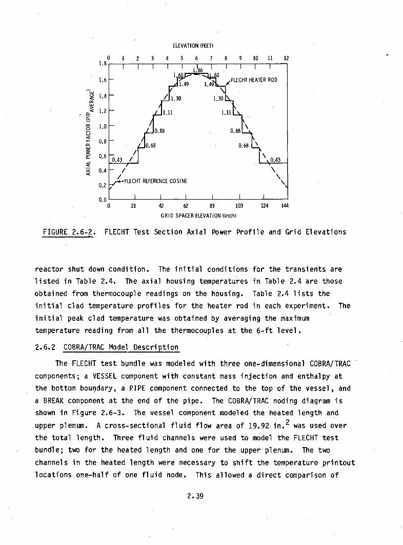
ELEVATION (FEET)
0 1 2 3 4 5 6 7 8 9 10 11 121.8 7 1 .1• ý6 1 1 1 1
1.6 1.49 1.49 FLECHT HEATER ROD
<0 1.4 /
< 1.2
0 1.0
' 0.8
0 . 0.43 0.40.4-/
FLECHT REFERENCE COSINE0.2
0 21 42 62 83 103 124 144
GRID SPACER ELEVATION (inch)
FIGURE 2.6-2. FLECHT Test Section Axial Power Profile and Grid Elevations
reactor shut down condition. The initial conditions for the transients are
listed in Table 2.4. The axial housing temperatures in Table 2.4 are those
obtained from thermocouple readings on the housing. Table 2.4 lists the
initial clad temperature profiles for the heater rod in each experiment. The
initial peak clad temperature was obtained by averaging the maximum
temperature reading from all the thermocouples at the 6-ft level.
2.6.2 COBRA/TRAC Model Description
The FLECHT test bundle was modeled with three one-dimensional COBRA/TRAC
components; a VESSEL component with constant mass injection and enthalpy at
the bottom boundary, a PIPE component connected to the top of the vessel, and
a BREAK component at the end of the pipe. The COBRA/TRAC noding diagram is
shown in Figure 2.6-3. The vessel component modeled the heated length and
upper plenum. A cross-sectional fluid flow area of 19.92 in. 2 was used over
the total length. Three fluid channels were used to model the FLECHT test
bundle; two for the heated length and one for the upper plenum. The two
channels in the heated length were necessary to shift the temperature printout
locations one-half of one fluid node. This allowed a direct comparison of
2.39

TABLE 2.4. Initial Condition for FLECHT Cosine Series Tests
Medium Flooding Rate High Flooding RateRun No. 00904 Run No. 04444
Upper Plenum 40 58Pressure (psia)
Initial Clad Temperature 998 1815at 6 ft (°F)
Rod Peak Power (kW/ft) 0.85 1.22
Flooding Rate (in./sec) 1.48 5.8
Coolant Temperature (OF) 128 155
Initial HousingTemperatures (°F)
0 ft 135 2732 ft 396 4334 ft 562 5335.5 ft 594 5556 ft 606 6176.5 ft 540 5097 ft 533 5107.5 ft 533 5068 ft 539 50410 ft 409 44112 ft 277 295lower plenum 115 150upper plenum 282 358
predicted temperatures to the experimental temperatures for all locations
above the 2-ft elevation, while keeping the bottom node at the bottom of the
experimental heated length. There were 14 fluid nodes in the vessel
component. A one-dimensional mesh was used in the test section since radial
distributions were believed to be insignificant. The node length was chosen
to allow comparison with measured data and yet maximize the time step size
allowed by the Courant limitations.
The 91 electrical heater rods were modeled by one average rod with the
average properties of all the heater rods. The test section housing was
modeled with a second rod with an inside heat transfer surface and an
2.40

PRESSURE BOUNDARYBREAK
COM PONENT
PI PECOM PONENT
SECTION 31 NODE 14 UPPER PLENUM
dx = 12 IN.
13
12
11
10
9
VESSEL SECTION 2COMPONENT 11 NODES 8
dx - 12 IN. HEATED LENGTH12 FEET
7
6
5
4
3SECTION 12 NODES
dx -9 IN. 1
tMASS FLOW & TEMPERATURE
BOUNDARY
FIGURE 2.6-3. COBRA/TRAC Model of FLECHT Test Section
2.41

insulated outer surface. The test rod was initialized with the axial power
profile shown in Figure 2.6-2 and the axial cladding temperature profile shown
in Table 2.5. The values in Table 2.5 were obtained by averaging all the
initial thermocouple readings (for a given elevation) presented in WCAP-8651
(Ref. 10). The housing was initialized with the axial temperature profile
presented in Table 2.4 and zero power generation. The vessel, pipe and break
components were initialized with saturated steam at the upper plenum pressure
and zero flow. A constant inlet flow and enthalpy boundary was applied at the
bottom of the vessel component. A pressure equal to the upper plenum pressure
given in Table 2.4 was specified for the break component at the top of the
vessel.
The reflood transient was run from a standing start with the initial
conditions mentioned above and the ANS +20% power decay curve as a forcing
function on the power level. The simulation continued until all levels in the
heated section were quenched.
TABLE 2.5. FLECHT Initial Cladding Temperatures
Elevation (Ave)ft
0.0
0.5
1.0
1.5
2.0
3.0
4.0
6.0
6.5
7.0
8.0
9.0
10.0
11.0
12.0
Medium Reflood RateRun No. 00904
OF
270
404
447
500
614
760
893
994
975
945
879
744
636
420
277
High Reflood RateRun No. 04444
OF
516
730
760
769
1031
1293
1557
1742
1716
1638
1507
1170
931
628
277
2.42
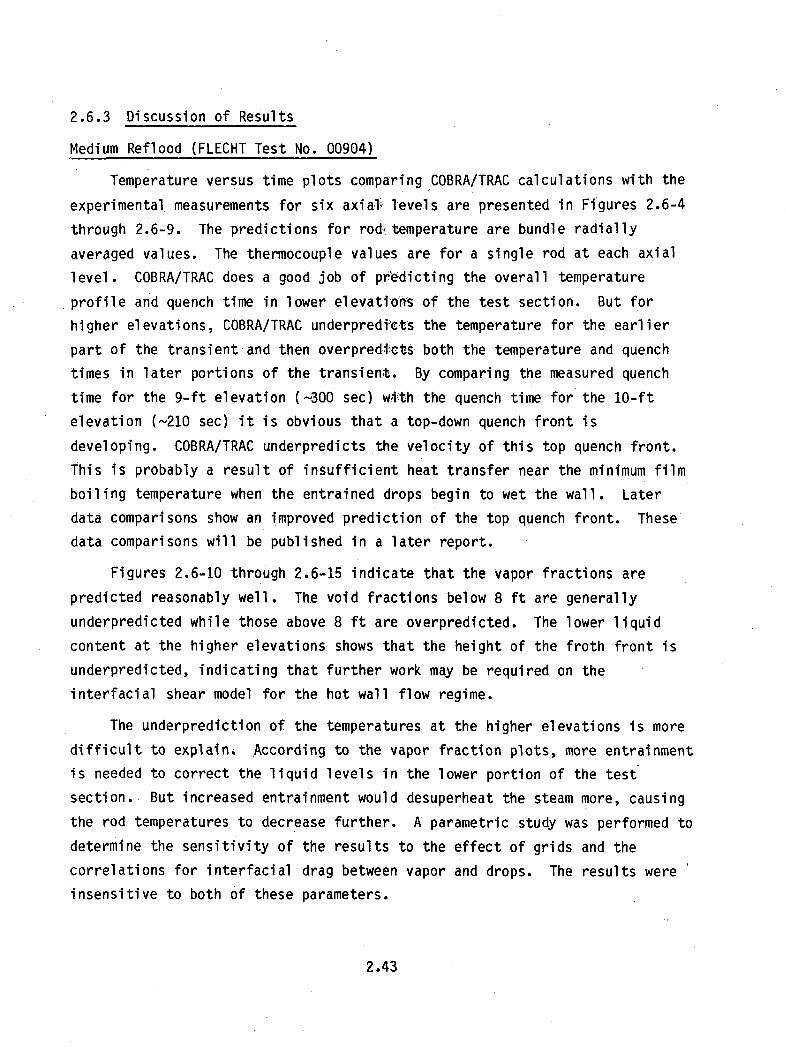
2.6.3 Discussion of Results
Medium Reflood (FLECHT Test No. 00904)
Temperature versus time plots compalring COBRA/TRAC calculations with the
experimental measurements for six axial levels are presented in Figures 2.6-4
through 2.6-9. The predictions for rod&temperature are bundle radially
averaged values. The thermocouple values are for a single rod at each axial
level. COBRA/TRAC does a good job of predicting the overall temperature
profile and quench time in lower elevatiohs of the test section. But for
higher elevations, COBRA/TRAC underprediet's the temperature for the earlier
part of the transient and then overpredilcts both the temperature and quench
times in later portions of the transient. By comparing the measured quench
time for the 9-ft elevation (~300 sec) with the quench time for the 10-ft
elevation (~210 sec) it is obvious that a top-down quench front is
developing. COBRA/TRAC underpredicts the velocity of this top quench front.
This is probably a result of insufficient heat transfer near the minimum film
boiling temperature when the entrained drops begin to wet the wall. Later
data comparisons show an improved prediction of the top quench front. These
data comparisons will be published in a later report.
Figures 2.6-10 through 2.6-15 indicate that the vapor fractions are
predicted reasonably well. The void fractions below 8 ft are generally
underpredicted while those above 8 ft are overpredicted. The lower liquid
content at the higher elevations shows that the height of the froth front is
underpredicted, indicating that further work may be required on the
interfacial shear model for the hot wall flow regime.
The underprediction of the temperatures at the higher elevations is more
difficult to explain. According to the vapor fraction plots, more entrainment
is needed to correct the liquid levels in the lower portion of the test
section. But increased entrainment would desuperheat the steam more, causing
the rod temperatures to decrease further. A parametric study was performed to
determine the sensitivity of the results to the effect of grids and the
correlations for interfacial drag between vapor and drops. The results were
insensitive to both of these parameters.
2.43

FLECHU COSINE SERIES TESTS
RUW N0 NO -009064-------
PEAK POWER 0.85 KW/FTREFLOOD RATE 1.48 IN/SEC
1600
r
U
U-
QrS
1200
... FLECHT-DATA 2 FT.-÷- COBRA-TF PREDICTION
1 . I m Il::1
800.
400.
G.0 60 120 180 240 300 360
TIME (SECONDS)
FIGURE 2.6-4.
2000
RUN
1600
1200
0
Temperature at 2-ft Elevation - FLECHT 00904
0 60 120 180 240 300 3c0
'IME (SFCONDS)
Temperature at 4-ft Elevation - FLECHT 00904FIGURE 2.6-5.
2.44
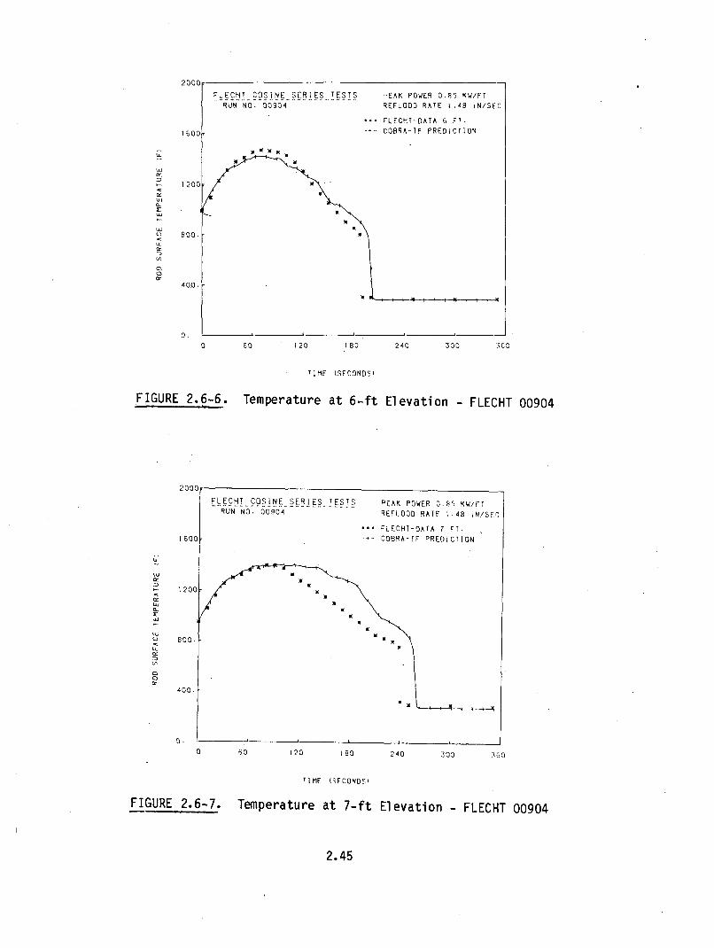
r4
Li-
0.60 120 180 240 300 5GO
TIME (SECONDS)
FIGURE 2.6-6.
2000
7L E(RU
1600
cc
- 1200
Boo.
Temperature at 6-ft Elevation - FLECHT 00904
0 60 120 180 240 200 30G
TIME (SECONDS,
FIGURE 2.6-7. Temperature at 7-ft Elevation - FLECHT 00904
2.45

2 r)r)n
RLECHT COSINESERIES TESTSRUN NO. 00904
'EAK POWER 0.25 KW/FT
REFLOOD RATE 1.48 IN/SEC
1600k
nr
cc
0r
12001
. FLECHT-DATA 9 PT.
COBRA-TF PREDICTION
800.
400.-
0 60 120 180 240 300 3cO
TIME (SECONDS)
FIGURE 2.6-8. Temperature at 9-ft Elevation - FLECHT 00904
PLECHT COSINE SERIES TESTSRUN A0. 00904
OEAK POWER O.R5 KW/FT
REFLOOD RATE 1.48 iN/SFC
., LECHT-DATA 10 PT..-- C0EORA-TF PREDICTION1600
W-rJ
0J
0q
1200
800.
400.
EKEKENIE
0.
0 60 120 180 240 300 3O0
TIME (SECONDS1
FIGURE 2.6-9. Temperat'dre at 10-ft Elevation - FLECHT 00904
2.46

1 .25
FLECHT COSINE SERIES TESTS
RUN NO. 00904
PEAK POWER 0.85 KW/FT
REFLOOD RATE 1.48 IN/SEC
... FLECHj-DATA 0-2 FT.- COBRA-TF PREDICTION.0of
0.75
0
0L
0.50
0.
0.
25ý
9 a
rin0 60 120 180 240 300 360
TIME (SECONDS)
Vapor Fraction at 0 to 2-ft Elevation for FLECHT 00904FIGURE 2.6-10.
I1.25,
.NLECHT COSINE.SERIES TESTSRUN NO. 030904
-EAK POWER 0.85 KW/FTREFLOOD RAIE 1.48 IN/SEC
- PLECHT-DATA 2-4 FT.- COBRA-IF PREDICTION
0.-75
E
M
0
Cro_
03
0L
0. 501
0.
0.
25
S 60 120 180 240 300 360
TIME (SECONDS)
FIGURE 2.6-11 Vapor Fraction at 2 to 4-ft Elevation for FLECHT 00904
2.47

0-
0•
60 120 18B 240 300 363
TIME (SECONDSJ
FIGURE 2.6-12. Vapor Fraction at 4 to 6-ft Elevation for FLECHT 00904
0
0_
0=
0 60 120 180 240 300 360
TIME (SECONDS)
Vapor Fractionz at 6 to 8-ft Elevation for FLECHT 00904FIGURE 2.6-13.
2.48
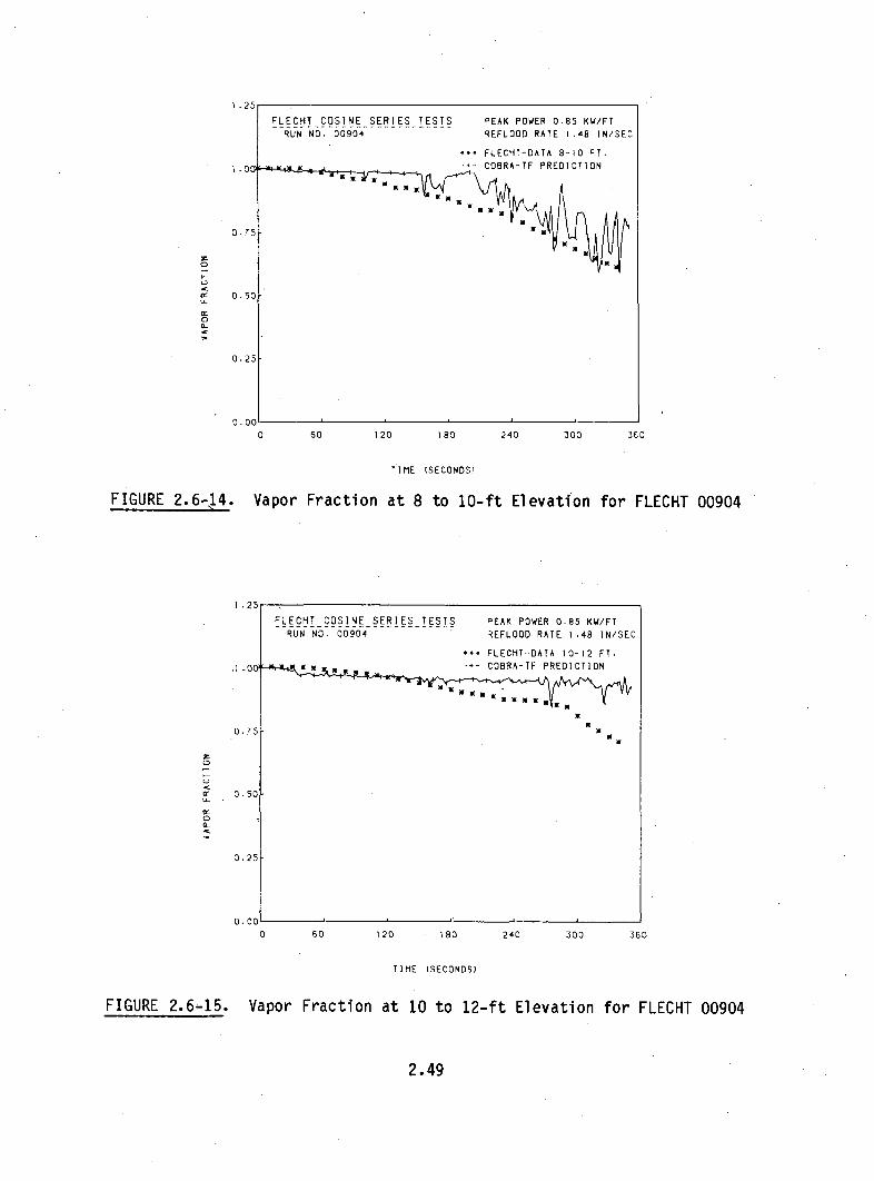
I .
RLECHT COSINESERIESTESTSRUN NO. 00904
'EAK POWER 0.85 KW/FT
REFLOOD RATE 1.48 IN/SEC
1 .00
0.75
... FLECHT-DATA 8-10 rT.
COBRA-TF PREDICTION
7-C_)
(_
0.50
0.25
q - r)nI0 60 120 180 240 300 360
TIME (SECONDS)
FIGURE 2.6-14. Vapor Fraction at 8 to 10-ft Elevation for FLECHT 00904
1 .25
.1 .00
0. 75
RLECHT COSINESERIES TESTSRUN NO. 00904
PEAK POWER 0.85 KW/FT
REFLOOD RATE 1.48 IN/SEC
. FLECHT-DATA 10-12 FT.
COBRA-TF PREDICTION
0c0-03CL
0. 50
0.25
Q. 00
0 60 120 180 240 300 360
TIME (SECONDS)
FIGURE 2.6-15. Vapor Fraction at 10 to 12-ft Elevation for FLECHT 00904
2.49
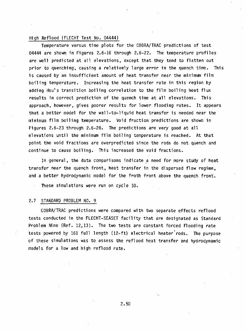
High Reflood (FLECHT Test No. 04444)
Temperature versus time plots for the COBRA/TRAC predictions of test
04444 are shown in Figures 2.6-16 through 2.6-22. The temperature profiles
are well predicted at all elevations, except that they tend to flatten out
prior to quenching, causing a relatively large error in the quench time. This
is caused by an insufficient amount of heat transfer near the minimum film
boiling temperature. Increasing the heat transfer rate in this region by
adding Hsu's transition boiling correlation to the film boiling heat flux
results in correct prediction of the quench time at all elevations. This
approach, however, gives poorer results for lower flooding rates. It appears
that a better model for the wall-to-liquid heat transfer is needed near the
minimum film boiling temperature. Void fraction predictions are shown in
Figures 2.6-23 through 2.6-28. The predictions are very good at all
elevations until the minimum film boiling temperature is reached. At that
point the void fractions are overpredicted since the rods do not quench and
continue to cause boiling. This increased the void fractions.
In general, the data comparisons indicate a need for more study of heat
transfer near the quench front, heat transfer in the dispersed flow regime,
and a better hydrodynamic model for the froth front above the quench front.
These simulations were run on cycle 10.
2.7 STANDARD PROBLEM NO. 9
COBRA/TRAC predictions were compared with two separate effects reflood
tests conducted in the FLECHT-SEASET facility that are designated as Standard
Problem Nine (Ref. 12,13). The two tests are constant forced flooding rate
tests powered by 161 full length (12-ft) electrical heater'rods. The purpose
of these simulations was to assess the reflood heat transfer and hydrodynamic
models for a low and high reflood rate.
2.50

0cc
0.
50 100 150 200 250 300
TIME (SFCONDS'
FIGURE 2.6-16. Temperature at 2-ft Elevation--FLECHT 04444
3000
RLECHT COSINE SERIES TESTSRUN NO. 04444
PEAK POWER 1 .2 KW/FT
REFLOOD RATE 5.P N/SE.C
...- LECHT-DATA 4 FT.
COBRA/TF PREDICTION
AVE. ROD TEMP.2400k
LU
1 Book
1 2o00
"M.
600.
0.0 50 100 150 200 250 300
TIME (SECONDS'
Temperature at 4-ft Elevation--FLEOHT 04444FIGURE 2.6-17.
2.51

Ul
0.
So 100 ISO 200 250 '30
TIME (SFCDNDS.
FIGURE 2.6-18. Temperature at 6-ft Elevation--FLECHT 04444
RLECHT COSINE SERIES TESTSRUN NO. 04444
PEAK POWER 1.22 KW/FTSEFLOOD RATE 5.R IN/SFC
... FLECHT-DATA 7 FT.
COBRA/IF PREDICTION
AVE. ROD TEMP.2400O
Lu
lqooý
E
IEE
WE
EE
E WE
12001
600.
X X~ xwE
0.
0 50 100 150 200 250 300
TIME (SFCONDS'
FIGURE 2.6-19. Temperature at 7-ft Elevation--FLECHT 04444
2.52

0
(r
050 100 150 200 ,S50 300
TIME 1SFCONDSI
FIGURE 2.6-20. Temperature at 8-ft Elevation--FLECHT 04444
RUNCHT COSINESERIES.TESTS
RUN NO. 044t4
PEAK POWER i.z2 KW/FT
REFLOOD RATE 5.P iN/SEC
• ILECHT-DATA 9 WT.
COBRA/TF PREDICTION
AVE. ROD TEMP.2400F
ST
r
ST
0
I 800k
12004
600.-
K KEEN
00 50 100 150 2 3 250 300
FIGURE 2.6-21.TIME (ICECONDS'
Temperature at 9-ft Elevation--FLECHT 04444
2.53

RULECHT. C0iNE SERIES TESTS
RUN NO. OA444
PEAK POWER I.- KW/FT
REFLOOD RATE 5.P iN/SFC
., LECHT-DATA 10 9T.
COBRA/TF PREDiCTiON
AVE. ROD TEMP.2400V
a:
0~
at
0
at
1800k
I200o
K KM K K
600.
1C.00.
0 50 100 150 200
T1ME ýEFCONDS'
FIGURE 2.6-22. Temperature at 10-ft Elevation--FLECHT 04444
-4 1 1 -
FLENT NCOSINE.SERIES E4TSRUN NO. 04444
PEAK POWER 1.22 KW/FT
REFLOOD RATE 5.8 IN/SEC
. FLECHT-DATA 0-2 FT.- COBRA-TF PREDICTION1 .00
0.75
0
0:
0. 50
0.25
U. 00 1
0 50 100 150 200 250 300
TIME (SECONDS)
FIGURE 2.6-23. Vapor Fraction at 0 to 1-ft Elevation--FLECHT 04444
2.54
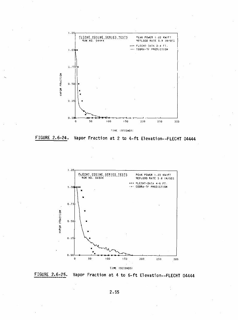
I •
FLECHT COSINE SERIES TESTS
RUN14 'NO . 0-4-4-44- - - - - - -PEAK POWER 1.22 KW/FT
REFLOOD RATE 5.8 IN/SEC
. FLECHI-DATA 2-4 FT.- COBRA-TF PREDICTION
1 .00
0.75
0.50 -U
z
0 I
0.251 *
0.00O0 50 100 150 200 250 300
TIME (SECONDS)
Vapor Fraction at 2 to 4-ft Elevation--FLECHT 04444FIGURE 2.6-24.
I •^•
I .00
R
mm
UCHT COSINE.SERIESTESTS.UN NO. 04444
PEAK POWER 1.22 KW/FTREFLOOD RATE 5.8 IN/SEC
. FLECHT-DATA 4-6 FT.--- COBRA-TF PREDICTION
0.75
0
W_0CL
0 .50 X
0 .25j
0. OC-0 50 00 1 50 200 250 300
TIME (SECONDS)
FIGURE 2.6-25. Vapor Fraction at 4 to 6-ft Elevation--FLECHT 04444
2.55
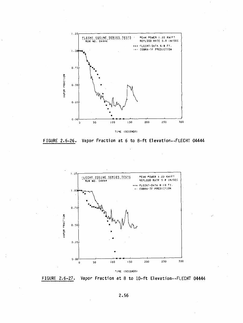
U-
0 50 100 150 200 250 300
TIME (SECONDS)
FIGURE 2.6-26.
1 .25
1.00
0.75
z
cr 0.50
w
Vapor Fraction at 6 to 8-ft Elevation--FLECHT 04444
0 50 100 150 200 250 300
TIME (SECONDS)
FIGURE 2.6-27. Vapor Fraction at 8 to 10-ft Elevation--FLECHT 04444
2.56

1 .25
FLECHT COSINE SERIES TESTS PEAK POWER 1.22 KW/FTS'NO. 04444 - -- REFLOOD RATE 5.8 IN/SEC
..., FLECHT-DATA 10-12 FT.
1.00 -- COBRA-TF PREDICTION
0. 75 mllu •
o Ko
0.50
0CL
0.25
0.00. K
0 50 100 150 200 250 300
']MIE (SECONDS)
FIGURE 2.6-28. Vapor Fraction at 10 to 12-ft Elevation--FLECHT 04444
2.7.1 Experimental Ddscription
A diagram of the FLECHT-SEASET test bundle is shown in Figure 2.7-1. The,
test section consisted of 161 electrical heater rods arranged in a square
pitch with dimensions comparable to 17x17-in. PWR fuel rod arrays. The rod
diameter was 0.374 in. and the rod pitch was 0.496 in. The bundle also
contained 16 control rod guide tubes of 0.484 in. diameter and 8 solid filler
.rods. The triangular filler rods reduced the excess flow area to within 5% ofthe power/flow area ratio of a PWR fuel assembly. The test section wasenclosed by a cylindrical stainless steel housing and was connected to an
upper and lower plenum. The housing has an inside diameter of 7.625 in. and
was insulated from the outside air to reduce the heat losses to the
environment. The bundle flow area was 23.945 in.2. The upper ends of both
the housing and test rods were bolted to the top of the test assembly. The
lower ends were allowed to hang free permitting axial movement. Horizontal
movement and/or bowing of the heater rods was restricted by 8 typical PWR grid
spacers located at 20.5 in. intervals, starting at the beginning of the heated
length.
2.57

SOLID FILLER
,•, 00000(
°0%0°8008000;~oo88oo 8\00 OOOQO0O0[
I000c?8o
HEATER ROD
FIGURE 2.7-1. FLECHT-SEASET Bundle Cross-Section
The electrical heater rods were constructed of a sp~iral-wound heating
element embedded in a magnesium oxide insulator. A chopped cosine power
profile was approximated by a seven-step power profile. The length of each
power step and the peak to average power factors are shown in Figure 2.7-2
along with the location of the 8 grid spacers.
The test assembly was initially heated by radiation from the heater rods
for more than an hour prior to reflood. During this heat-up phase the rods
were surrounded by stagnant steam and all rods had a constant peak power of
0.8 kW/ft. These conditions were maintained until the desired peak clad
temperature of 16000F was obtained. Water was injected into the lower plenum
with a constant flow rate, an inlet temperature of 1270F, and a pressure of 40
psia. When the rising water reached the beginning of the heated length, the
constant rod power was converted to the ANS +20% decay heat rate for the
reflood portion of a LOCA. The initial test parameters for both the high and
low flooding rate experiments have been tabulated in Table 2.6.
The initial temperatures for all axial levels were computed by averaging
the thermocouple temperatures at a given elevation. Two heater rods were
2.58

ELEVATION (FEET)
0 1 2 3 4 5 6 7 8 9 10 11 121.8
1.6
1.4
!a 1.2
1.0
0 0.8
0 0.6
0.4
0.2
00 21 42 62 83 103 124 144
GRID SPACER ELEVATION (inch)
FIGURE 2.7-2. FLECHT-SEASET Axial Power Profile and Grid Locations
TABLE 2.6. Test Parameters for Standard Problem No. 9
High Flooding(Run No. 31701)
Low Flooding(Run No. 31805)
Forced injectionrate into bundle
Pressure attop of bundle
Injection watertemperature
Initial power at6 ft elevation
Initial rodtemperatures (ave)
6 in./sec 0.8 in./sec
40 psia 40 psia
127 0F127 0F
0.7 kW/ft 0.7 kW/ft
02468
1012
ftftftftftftft
430°F747°F1275°F1561 0 F1327 0F836 0 F600°F
02468
1012
ftftftftftftft
430°F751 0 F1274 0F1560 0 F1324 0 F839 0 F600°F
2.59
inoperative during the entire transient, therefore the rod temperature in the
immediate vicinity of the unpowered rods and those near the housing were
eliminated from the initial temperature averaging.
2.7.2 COBRA/TRAC Model Description
The FLECHT-SEASET test assembly was modeled with three COBRA/TRAC
components; a one-dimensional VESSEL component with mass injection at the
bottom boundary, a PIPE component connected to the top of the vessel, and a
BREAK component on the end of the pipe. The COBRA/TRAC nodalization is shown
in Figure 2.7-3. The vessel component modeled the heated length and upper
plenum. A fluid flow area of 24.16 in. 2 was used for the simulation. (This
area was calculated from pretest information and was approximately 0.6%
greater than the actual flow area of 23.945 in.2.) The vessel was modeled
using three channels, two for the heated length and one for the upper
plenum. Two channels in the heated length were necessary to match the
COBRA/TRAC temperature output locations with those presented in the
experimental data. There were 14 fluid nodes in the vessel component. The
159 functioning heater rods were modeled with one average rod. The test
section housing was modeled by a tube rod with an inside heat transfer surface
and an insulated outer surface. A one-dimensional mesh was used since it was
thought that no significant radial profiles existed in the experiment. This
turned out to be an erroneous assumption for the low flooding test since
significant radial vapor temperature distributions were measured in the
experiment.
The COBRA/TRAC heater rod was initialized with the axial temperature
profile of Table 2.6 and the axial power profile of Figure 2.7-2. The peak
power was 0.7 kW/ft. The housing was initialized with the axial temperature
profile and zero power generation. The vessel, pipe and break components were
initialized with saturated steam at 40 psia. A constant flow boundary
condition of 127°F water was specified at the bottom of the vessel. At the
break, a pressure boundary of 40 psia was specified.
The reflood transient was run from a standing start, with the initial
conditions listed in Table 2.6 and the ANS +20% power decay curve. The
simulation continued until all levels of the heated section were quenched.
2.60

BREAK PRESSURE BOUNDARY
COM PONENT
PIPECOM PONENT
SECTION 3I NODE 14 UPPER PLENUM
dx = 12 IN.
13
12
11
joI.0
9
VESSEL SECTION 2COMPONENT 11 NODES 8
dx - 12 IN. - HEATED LENGTH12 FEET
7
6
5
4
3SECTION 1 22 NODES
dx = 9 IN.
tMASS FLOW & TEMPERATURE
BOUNDARY
FIGURE 2.7-3. COBRA/TRAC Model of FLECHT-SEASET for Standard Problem No. 9
2.61

2.7.3 Discussion of Results
Low Reflood (FLECHT-SEASET Test No. 31805)
Temperature versus time plots comparing the COBRA/TRAC predictions at the
various axial levels are shown in Figures 2.7-4 through 2.7-8. Temperatures
calculated by COBRA/TRAC are compared to the measurements for one rod (this
was the only data available). The temperature plots show that COBRA/TRAC does
a good job of predicting the temperatures in the lower end of the test
section, but temperatures are underpredicted in the higher elevations. More
recent simulations have shown that radial temperature distributions have a
significant effect on clad temperatures in the upper part of the bundle and a
much better data comparison can be obtained by using more than one channel to
model the test section. Void fraction comparisons are shown in Figures 2.7-9
through 2.7-20. The predictio~ns are very good at all elevations, indicating
that the models for liquid entrainment and interfacial shear are reasonably
accurate.
High Reflood (FLECHT-SEASET Test No. 31701)
Temperatures versus time plots comparing the COBRA/TRAC prediction at the
measured data at five axial levels are presented in Figures 2.7-21 through
2.7-25 No experimental data were available for this report, but they seem to
follow the same general trends as those for FLECHT 04444 (Section 2.6), a test
with approximately the same test conditions. The higher reflood rate,
(6 in./sec) quenches all elevations in less than 150 seconds. If the same
trends as those for FLECHT 04444 hold for the FLECHT-SEASET high reflood rate,
COBRA/TRAC should be able to predict the peak temperatures at all elevations,
but with an increasing overprediction for quench times at the higher axial
elevations. The quench time predictions would probably improve if the
simulation was rerun with the heat transfer improvements to the minimum film
boiling temperature region.
These simulations were run on cycle 10 of COBRA/TRAC.
2.62
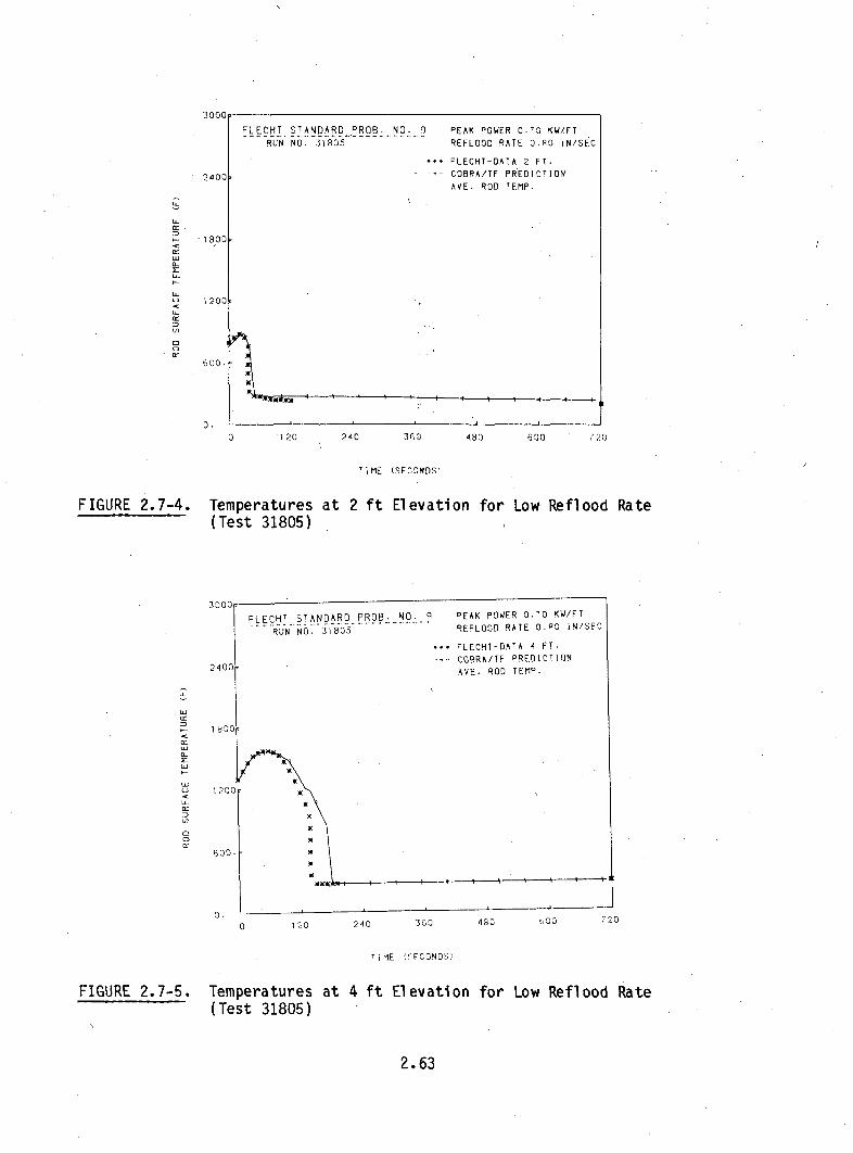
.100 cl
24001
0W
W
ft.
1 800ý
FLECHT STANDARD PROB..N.O-. 9 PEAK POWER 0.70 KW/FTRUN NO. 31805 REFLOOD RATE D.A0 iN/SEC
- LECHT-DATA 2 FT.
COBRA/TF PREDICTION
AVE. ROD TEMP.
F •
1200
600,
t
0 120 240 360 480 600 '20
TIME ISECONDS)
FIGURE 2.7-4. Temperatures(Test 31805)
at 2 ft Elevation for Low Reflood Rate
3000f
FLECHT STANDARD PROB. NO. .q PEAK POWER 0.'0 KW/FTRUN NO. 31805 REFLOOD RATE D.A0 iN/SEC
FLECHT-DATA 4 FT.COBRN/TF PREDICTIONAVE. ROD TEMP.2400
.-
U-
a:
0
0r
I 8001
1200 YA
600.
¶
10 200 4 8 0C 2 0
TiME C'FICONDS.
FIGURE 2.7-5. Temperatures at 4 ft Elevation for Low Reflood Rate(Test 31805)
2.63
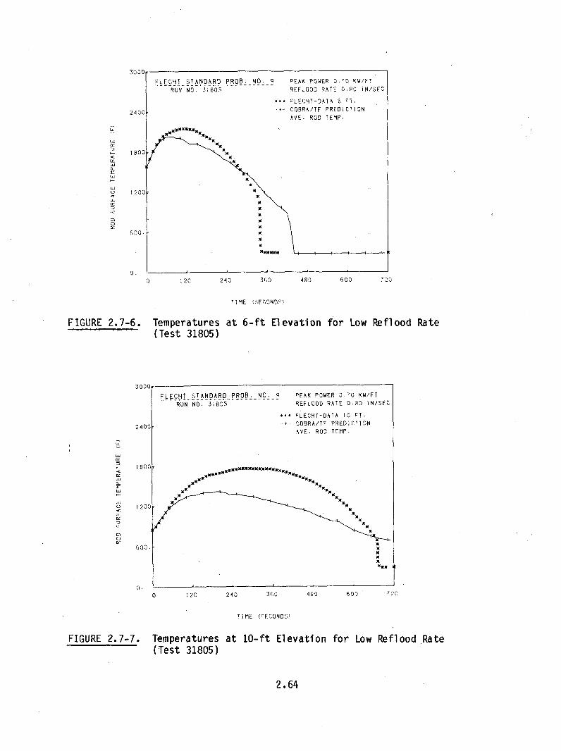
0-
:D
C
0.
0 120 240 3G0 480 600 720
TIME U2ECONDOý
FIGURE 2.7-6. Temperatures at 6-ft Elevation(Test 31805)
for Low Reflood Rate
I
FLECHT STANDARD PROB. NO qRUN NO. 31805
PEAK POWER 0.'0 KW/FTREFLOOD RATE 0.60 !N/SEC
2404
0~
CDW-
1800
.. ,, LECHT-DATA 10 FT.-+-COBRA/TF PREDICTION
AVE. ROD TEMP.
xx N(X)Nx
X )K WX Xx x
1 200
600-
0.0 120 240 3GO 480 600 720
TIME (fECONDSI
FIGURE 2.7-7. Temperatures(Test 31805)
at 10-ft Elevation for Low Reflood Rate
2.64
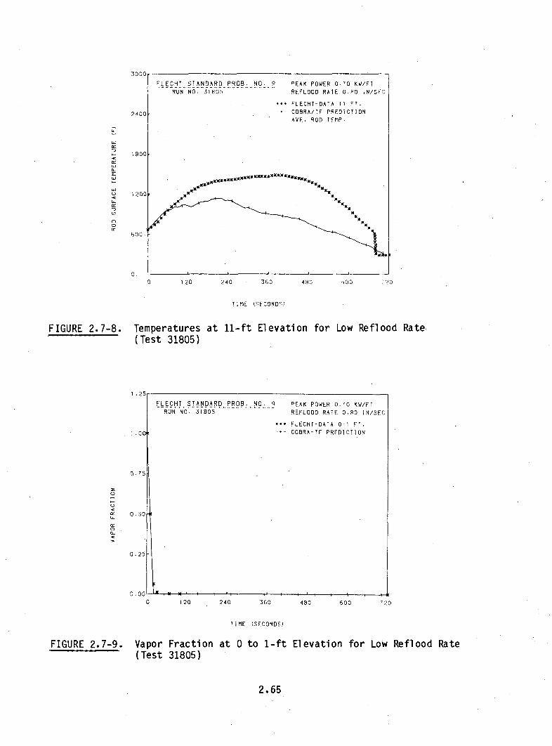
uJ
2,
0C
120 240 360 480 '0 0 120
TIME (SECONDV.
FIGURE 2.7-8. Temperatures(Test 31805)
at 11-ft Elevation for Low Reflood Rate.
FLERUT STANDARD PROB. NO.RUN NO. 31805
PEAK POWER 0.'0 KW/FTREFLOOD RATE 0.80 IN/SEC
... FLECHT-DATA 0-i FT.- COBRA-TF PREDICTION1 .00
0.75
M
0
CL
0.50
0.25
UU .- - i . i 4 -
0 120 240 360 480 600 720
TIME (SECONDS)
FIGURE 2.7-9. Vapor Fraction(Test 31805)
at 0 to 1-ft Elevation for Low Reflood Rate
2.65

I I25.
z•a-
0L
0-
FLECH. STANDARD PROB. NO. 9 PEAK POWER o.'o KW/FTRUN NO. 31805 REFLOOD RATE 0.80 !N/SFC
... PLECHT-DATA 1-2 FT.1 .0 -. COBRA-TF PREDiCTION
0.75 m
0.50
0.25
0.000 120 240 360 480 600 720
TIME (SECONDS)
FIGURE 2.7-10. Vapor Fraction at(Test 31805)
1 to 2-ft Elevation for Low Reflood Rate
1 .25
1 .00
0. 75
FLECHT STANDARD PROB. NO.39
RUN NO. 31805PEAK POWER 0.70 KW/FT
REFLOOD RATE O.R0 iN/SEC
... FLECHT-DATA 2-3 FT.'.-- COBRA-TF PREDICTION
0
L:
a:0.50
3K
Ix
0.25
-.- j.-- .
0 120 240 360 480 600 720
TIME (SECONDS?
FIGURE 2.7-11. Vapor Fraction at 2 to 3-ft Elevation(No. 31805)
for Low Reflood Rate
2.66

I .
0.
0a-
0.
0.
0.120 240 360 480 6300
TIME (SFCONDS.
FIGURE 2.7-12.
a:a-.
Vapor Fraction(Test 31805)
at 3 to 4-ft Elevation for Low Reflood Rate
0.",
0. (
0,251
120 240 360 480 ,00
'IME (E CONOND
FIGURE 2.7-13. Vapor Fraction at 4 to 5-ft Elevation(Test 31805)
for Low Reflood Rate
2.67
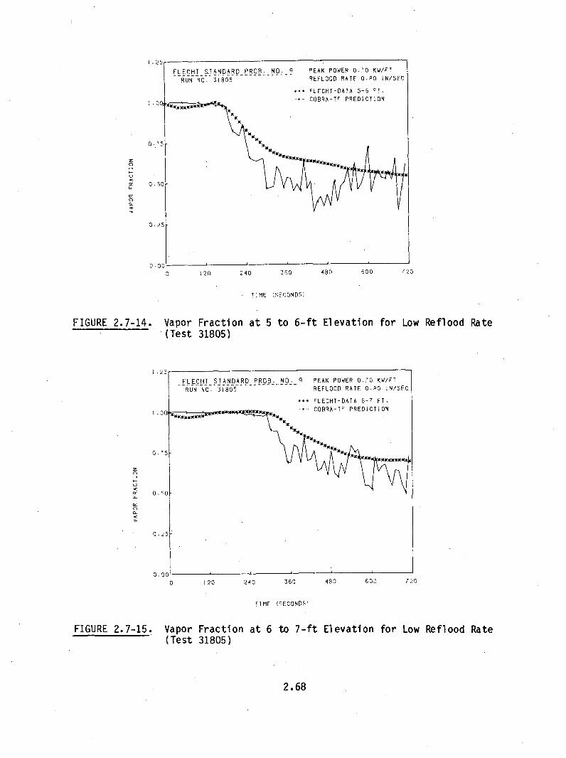
. 2 5f
0.
C-
0.120 240 360 480 600 720
TIME (SECONDS'
FIGURE 2.7-14.
0
a-
Vapor Fraction at 5 to 6-ft Elevation for Low Reflood Rate(Test 31805)
0 120 240 360 480 600 720
TIME (SECONDS'
FIGURE 2.7-15. Vapor Fraction at 6(Test 31805)
to 7-ft Elevation for Low Reflood Rate
2.68

-FLECHI .STANDA.RD .PROB-. NO-.- P EAK POWER 0.'0 KW/FT
RUN NO. 31805 REFLOOD RATE OGPO iN/SEC
... rLECHT-DATA 7-8 :T.
S..COBRA-TF PREDICTIONEl u. - . i
V-ý
0 . 75
2:
0
0
0 . 0
0. 25
0.00.120 240 3c0 430 600
T1ME ISECONDS'
FIGURE 2.7-16.
2:0
Vapor Fraction at 7(Test 31805)
to 8-ft Elevation for Low Reflood Rate
0 120 240 360 480 630 720
TIME (SECONDSI
FIGURE 2.7-17. Vapor Fraction(Test 31805)
at 8 to 9-ft Elevation for Low Reflood Rate
2.69

- 2 5 rFLECHT STANDARD PROB. NO. q PEAK POWER 0.70 KW/FT
RUN NO. 31805 REFLOOD RATE ORO iN/SEC
. FLECHT-DATA 9-10 FT.
0. '51
0
CL
,U0.
0 .25
Ub0 120 240 300 480 600 720
TIME (SFCONDS;
FIGURE 2.7-18. Vapor Fraction(Test 31805)
at 9 to 10-ft Elevation for Low Reflood Rate
1 .25
FLECHT STANDARD PTRUd N NO.- 3-1-80-5------
OB. NO. q PEAK POWER 0. 0 KW/FT
REFLOOD RATE 0R0 IN/SFC
... FLECHT-DATA 10-11 FT.• • . "+- A-.I P•ED1CTJON
. 0 -1 ------------
0CL
0. -
0.,
0. '10 . 1 20 240 300 480 600 720
TIME (SECONODS1
FIGURE 2.7-19. Vapor Fraction(Test 31805)
at 10 to 11-ft Elevation for Low Reflood Rate
2.70
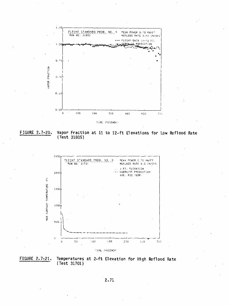
- --r
1 .O0
0. '5
FLECH. STANDA RD PROB. NO. Q PEAK POWER 0-'0 KW/FTRUN NO. Z31805 REFLOOD RATE O.PO iN/SEC
rLECHT-DATA 11-12 FT.
E1PRloci
cc
0'C
0.,0
0.251
FIGURE 2.7-20.
w
0,-00! 1
0 1 20 240 300 480 600
TIME I'EC0NDF?
Vapor Fraction at 11 to 12-ft Elevations for L(Test 31805)
2500
LECHT ..STANDARDPROB.O...NO..• PEAK POWER 0.10 KW/FT
RUN NO. 31701 REFLOOD RATE 6.0 IN/SFC
. FT. ELEVATION
2000, COBRA/TF PREDICTIONAVE. ROD TEMP.
1500
1000
500.
.ow Reflood Rate
v-
0 50 100 150 200 250 333
T1ME 6F,.CONDT'
FIGURE 2.7-21. Temperatures at 2-ft Elevation for(Test 31701),
High Reflood Rate
2.71

C-
00r
0.
0 50 100 I50 200 250 300
TIME (IFCONDS'
FIGURE 2.7-22. Temperatures(Test 31701)
at 4-ft Elevation for High Reflood Rate
2 ýQOF
RLECHNT STANDARD PROB. NO.RUN NO. 3170i
PEAK POWER 0.'0 KW/FT
REFLOOD RATE 6.0 iN/SF(
2000k
C FT. ELEVATION
COBRA/TF PREDICTION
AVE. ROD TEMP.
Ujw
cc
1500
IO000O
500o.
s 50 100 150 200, 250 300
TIME (7FCONDS'
FIGURE 2.7-23. Temperatures at 6-ft(Test 31701)
Elevations for High Reflood Rate
2.72

,ýOuuý
RN SN.0TANDARDPROB.NO.RUN NO. 31701
PEAK POWER 0.'0 KW/FT
REFLOOD RATE 6.0 iN/SFr
R rT. ELEVATION
COBRA/TF PREDICTION
AVE. ROD TEMP.2004
CL
0r
10
500.
0 50 .100 1 50 200 250 :300
TiME (F.FC0NDF'
FIGURE 2.7-24. Temperatures(Test 31701)
at 8-ft Elevation for High Reflood Rate
ý,.,)nn,
RLECH 0STANDARD PROB. NO.RUN NO. 31701
PEAK POWER 0.'0 KW/FT
REFLOOD RATE 6.0 iN/SFC
2000C
a-I_
0W-
1 500ý
iO FT. ELEVATION
COBRA/TF PREDICTIONAVE. ROD TEMP.
1 000
500.
0.
0 50 100 150 200 250 300
TIME (SECONDS'
FIGURE 2.7-25. Temperatures at 10-ft Elevation(Test 31701)
for High Reflood Rate
2.73

2.8 NRU NUCLEAR FUEL ROD FORCED REFLOOD EXPERIMENT
This LOCA test series was run in the National Research Universal (NRU)
reactor at Chalk River, Ontario, Canada. The tests were conducted by PNL for
the NRC to evaluate the thermal-hydraulic and mechanical deformation behavior
of a full-length nuclear rod bundle during the heatup, reflood, and quench
phases of a loss-of-coolant accident (LOCA). Two tests, PTH110 and TH214,
(Ref. 14,15) were selected for COBRA/TRAC simulation to assess the
applicability of the heat transfer and hydrodynamic models in the code
(including the fuel rod gap conductance model) to reflood in nuclear fuel
bundles. Test PTH110 was a constant forced bottom reflood experiment and test
TH214 was a variable flow rate bottom %reflood experiment. These two tests are
representative of the approximately '55 experimental tests conducted in the NRU
facility.
2.8.1 Experimental Description
The NRU test train was 30 ft 1-1/2 in. in length and consisted of six
major sections; the inlet region, test bundle, shroud, outlet region, hanger
and closure head. The entire test train was inserted into a 25-ft pressure
tube inside the NRU reactor. The closure region provided the pressure
boundary between the test train and the NRU pressure tube. A schematic of the
NRU test train is shown in Figure 2.8-1. The hanger tube suspended the test
bundle and shroud from the closure head. The 14-ft long stainless steelshroud, constructed from two halves clamped together at 7-in. intervals,
supported the test bundle.
The fuel bundle consisted of a 6x6 segment of a 17x17 PWR assembly design
with the four corner rods removed for easier insertion in the shroud. A
cross-section of the test section is shown in Figure 2.8-2 The outer ring of
16 rods plus the corner rods of the next inner ring served as guard rod
heaters during the tests. The central 11 rods and instrument thimble (inside
the dotted line in Figure 2.8-2) arranged in a cruciform pattern were the test
rods of interest. All rods were unpressurized for both tests. The nuclear
fuel rods had a cladding O.D. of 0.379 in. and pellet diameter of 0.325 in.
The rod-to-rod pitch was 0.502 in. and the chopped cosine power profile had a
peak power of 0.55 kW/ft at the 6-ft elevation.
2.74

APPROXIMATELYNRU ELEV (482'-01)
CLOSURE
TEST HANGER TUBE
-BULK OUTLET TEMPERATUREINDI CATORS
FLUX MONITORS
NRU ELEV (467'-0")
FUELBUNDLE
NRU ELEV (455'-W")
SHROUD
CLADDING THERMOCOUPLESAT VARIOUS LOCATIONS ON FUEL RODS
'BULK INLET TEMPERATUREINDICATORS
APPROXIMATELYNRU ELEV (452'-0")
FIGURE 2.8-1. Vertical Test Train Configuration for NRU Reflood Experiments
2.75

PRESSURE TUBETE STT 0
'~FUEL RODE 0 Q 0100 SHROUD
GUARD T(HOMBoo,FUEL ROD :O00 e0K
-4.070"
FIGURE 2.8-2. NRU Test Bundle Cross-Section
Horizontal movement and/or bowing was restricted by seven typical PWR
grid spacers at 21-in, intervals, starting at the beginning of the heated
length. The shroud was insulated on the outer surface to reduce the amount of
heat loss to the environment.4
The experimental test conditions were obtained in two steps: a steady-
state phase and a transient phase. During the steady-state phase, the rod
power was slowly increased to the desired value for the particular test while
the dry steam coolant flow rate was decreased to produce a peak cladding
temperature of 8000F., The steady-state conditions were maintained at these
values until the thermocouple readings stabilized. The transient was then
initiated. The steam coolant flow was stopped as quickly as possible, then
reflood was started at the desired flow rate. The time period between steam
shut-off and reflood initiation was an adiabatic heatup period and was allowedto continue until the specified maximum peak cladding temperature wasreached.
When the injected water reached the bottom of the heated length of the
fuel rods, a quench front formed with significant vapor generation. The steam
2.76

and entrained water droplets flowing through the test section provided
adequate cooling for the test assembly. This two-phase mixture of steam and
droplets continued out the top of the heated length and into the hanger
region. Here the drops de-entrained and a top-down quench front could develop
if the right conditions existed. The de-entrained liquid remained directly
above the test bundle and could fall back into the bundle if the vapor
velocities were sufficiently low. Reflood was continued until all levels ofthe heated length had quenched. The test parameters for PTH110 and TH214
(Ref. 16,17) have been tabulated in Table 2.7.
TABLE 2.7. Initial and Boundary Conditions for NRU Tests PTH110 and TH214
PTH110 TH214
Initial Peak Rod Temp.(Start of Transient) OF 848 800
Peak Rod Power kW/ft 0.55 0.55
Reflood Rate in./sec Constant Variable (computer(Duration Time) sec 2.1 controlled)
2.18 for (54) sec1.42 for (15) sec0.89 for (24) sec1.36 for (16) sec0.54 for (136) sec0.74 for (14) sec0.51 for (72) sec
Inlet CoolantTemperature OF -100 -127
Reflood Delay Time sec 32 7
System Pressure psia 40 40
2.77
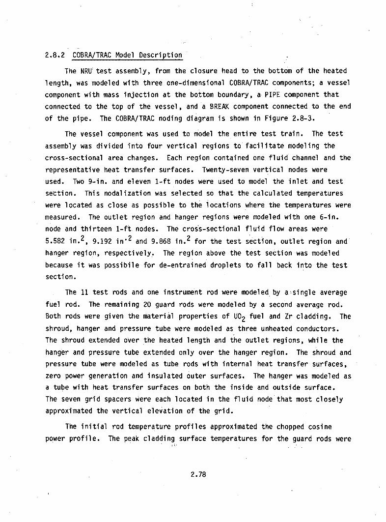
2.8.2 COBRA/TRAC Model Description
The NRU: test assembly, from the closure head to the bottom of the heated
length, was modeled with three one-dimensional COBRA/TRAC components; a vessel
component with mass injection at the bottom boundary, a PIPE component that
connected to the top of the vessel, and a BREAK component connected to the end
of the pipe. The COBRA/TRAC noding diagram is shown in Figure 2.8-3.
The vessel component was used to model the entire test train. The test
assembly was divided into four vertical regions to facilitate modeling the
cross-sectional area changes. Each region contained one fluid channel and the
representative heat transfer surfaces. Twenty-seven vertical nodes were
used. Two 9-in. and eleven 1-ft nodes were used to model the inlet and test
section. This nodalization was selected so that the calculated temperatures
were located as close as possible to the locations where the temperatures were
measured. The outlet region and hanger regions were modeled with one 6-in.
node and thirteen 1-ft nodes. The cross-sectional fluid flow areas were
5.582 in.2, 9.192 in"2 and 9.868 in. 2 for the test section, outlet region and
hanger region, respectively. The region above the test section was modeled
because it was possibile for de-entrained droplets to fall back into the test
section.
The 11 test rods and one instrument rod were modeled by alsingle average
fuel rod. The remaining 20 guard rods were modeled by a second average rod.
Both rods were given the material properties of U02 fuel and Zr cladding. The
shroud, hanger and pressure tube were modeled as three unheated conductors.
The shroud extended over the heated length and the outlet regions, while the
hanger and pressure tube extended only over the hanger region. The shroud and
pressure tube were modeled as tube rods with internal heat transfer surfaces,
zero power generation and insulated outer surfaces. The hanger was modeled as
a tube with heat transfer surfaces on both the inside and outside surface.
The seven grid spacers were each located in the fluid node that most closely
approximated the vertical elevation of the grid.
The initial rod temperature profiles approximated the chopped cosine
power profile. The peak cladding surface temperatures for the guard rods were
2.78

BREAKCOMPONENT
PI PECOMPONENT
VESSELCOMPONENT
13 NODESdx = 12 IN.
1 NODEdx =6 IN.
11 NODESdx =12 IN.
2 NODESdx = 9 IN.
PRESSURE BOUNDARY
I27
26
25
24.
23:..
22 1222120
19
18
17
1615
CLOSURE HEAD REGION
HANGER REGION
OUTLET REGION
TEST REGION
14.-.13 1312
11
10
9_ 8 "
7
65
43 - - 1
MASS FLOW ANDTEMPERATURE BOUNDARY I NLET REGION
FIGURE 2.8-3. COBRA/TRAC Model of NRU Test Section
2.79

1321°F for test PTH11O and 990VF for test TH214. The peak central test rod
temperatures were initialized at 1330°F for test PTH110 and 945 0 F for TH214.
The shroud temperature increased linearly from the 275 0 F at the inlet region
to 595 0 F at the outlet region, and the hanger and pressure tube temperatures
were initialized at the test bundle outlet steam temperature of 596 0 F.
The vessel, pipe and break were all initialized with saturated steam at
40 psia. A constant average power with a chopped cosine power profile was
applied to all rods. The appropriate flow boundary conditions were applied at
the bottom of the vessel component. The simulation was run until all
elevations had quenched.
2.8.3 Discussion of Results
Constant Reflood Rate Test (PTH110)
Figures 2.8-4 through 2.8-11 show the computed and experimental guard rod
temperatures plotted versus time for eight axial locations. The NRU
temperature data was averaged for all guard rod thermocouples at a particular
axial location. Where the axial node locations in the computational model did
not coincide exactly with axial temperature measurement locations, the
COBRA/TRAC results were compared to the nearest thermocouple locations. In
all cases the measured locations were within 4 to 6 in. of the computed
levels. Computations for the 7-ft elevation were compared against
measurements at both the 6.4-ft and 8.1-ft elevations. The COBRA/TRAC 7-ft
values for temperatures and quench time were of the proper magnitude.
At nearly all elevations the prediction is within 50OF of the average
guard rod peak temperature and within 100*F of the individual rod temperature,
over the heated length. Exceptions to this are the 6-ft elevation, (compared
in Figure 2.8-8 to the 6.36-ft NRU data) and the prediction at the 10-ft
elevation, (compared in Figure 2.8-11 to the 9.86-ft NRU data) where the
predicted temperatures differ somewhat from the NRU data. The early quench
predicted at the 6-ft elevation is probably due to using a lower elevation in
the calculation than the thermocouple's position, because comparisons at both
the 5-ft and 7-ft elevations are very good. The inability to predict the
2.80

U-
Lu
c?
0 50 100 150 200 • 250 300
TIME (SECONDS)
FIGURE 2.8-4. Temperatures at the 1.12-ft Elevation (Test PTH110)
NRU UNPRESSURI2EO TESTRUN NO. PTH~lO
PEAK POWER O.S5 KW/FTREFLOOD RATE VARIABLE
2000
U?
0~i2,
1 500
1000
500
*.. NRU-DATA 3.3 FT.COBRA-TF 3.0 FT. ELEV.
AVE. GUARD ROD TEMP.
Sli M i Mw mw il( m Il N. jl M I(W
E
0a 50 100 150 200 250 300
TIME (SECONDSI
FIGURE 2.8-5. Temperatures at the 3.0-ft Elevation (Test PTH110)
2.81

NRU UNPRESSURIZED TESTRUN NO. PTH11O
PEAK POWER 0.55 KW/FT
REFLOOD RATE VARIABLE
... NRU-DATA 4.03 FT.
COBRA-TF 4.0 FT. ELEV.
AVE. GUARD ROD TEMP.2000V
w
uJ
n
0C
1500
1000
0
WN
w
)K
N
0 50 100 150 200 250 300
TIME (SECONDS)
FIGURE 2.8-6.
2500
2000
U-
- 1500
1000
0Ir.
Temperatures at the 4.0-ft Elevation (Test PTH11O)
50 100 150 200 250 300
TIME (SECONDS)
FIGURE 2.8-7. Temperatures at the 5.0-ft Elevation (Test PTH11O)
2.82

L:
Ujir
cr0j
(1
0 50 100 150 200 250 300
TIME (SECONDS,
FIGURE 2.8-8.
2500-
2000
U-
an
1- 1500
LLJU,
COO0c
c:
Temperatures at the 6.0-ft Elevation (Test PTH110)
00 50 100 150 200 250 300
TIME (SECONDS)
FIGURE 2.8-9. Temperatures at the 7-ft Elevation (Test PTH110)
2.83

U-
LU
wSU
C5
B
0r
00 50 100 150 200 250 300
TIME (SECONDS)
FIGURE 2.8-10. Temperatures at the 8.0-ft Elevation (Test PTH110)
NRUNUNPRESSURIOZEDTESTRUN NO. PTH110
PEAK POWER 0.55 KW/FTREFLOOD RATE VARIABLE
• NRU-DATA 9.86 FT.-.- COBRA-TF 10.0 FT. ELEV.
AVE. GUARD ROD TEMP.2000F
US
CL
1500 NNNNNN~N
MN
NN
NN
NN
1000
500 -
00 so 100 150 200 250 300
TIME (SECONDS)
FIGURE 2.8-11. Temperatures at the 10.0-ft Elevation (Test PTH110)
2.84

quench time and temperature at the 10-ft elevation has been attributed to the
absence of an accurate top-down quench model. A recent simulation using an
improved top quench front model shows a markedly improved comparison at the
10 ft elevation. This simulation will be presented in a later report.
As was seen in the temperature profiles, COBRA/TRAC predicts the quench
times for all elevations, except the 10-ft elevation, to within 10 to 15 sec
of the NRU predictions. The results presented above are excellent for bottom
reflood and quenching in a nuclear fuel bundle.
Variable Reflood Rate Test (TH214)
The plots of computed and experimental rod temperatures versus time for
the same 8 axial locations as for test PTH110 are presented in Figures 2.8-12
through 2.8-19. As was the case with PTH110, all the NRU data is average
guard rod information. COBRA/TRAC underpredicts the temperature profile and
quench times in the 3- to 5-ft region ( Figures 2.8-13 through 2.8-15). The
code underpredicts the peak temperatures while overpredicting the quench time
for the 6-ft elevation (Figure 2.8-16). The uncertainty in the magnitude of
the rapidly varying inlet flow rate and temperature is partially responsible
for the poor data comparison in the test region below 6 ft.
Figure 2.8-17 compares the 7-ft prediction against the 6.4-ft and the
8.1-ft NRU test results. The fact that the 6.4-ft elevation quenched and 8.1-
ft elevation did not quench indicates that the quench front stabilized
somewhere between the two data locations. Therefore, if the COBRA/TRAC inlet
condition was different than actual inlet conditions, a stable quench front
would occur at a different location. By comparing the COBRA/TRAC results for
the 6-ft to the 7-ft elevation, it appears that the predicted quench front
stablized closer to the 6-ft elevation rather than the 6.5 to 8.0-ft elevation
presented by the data. Even though the quench front location was
underpredicted, this had little effect on the temperatures above the 7-ft
elevation, which would indicate that the entrainment rate and interfacial heat
transfer is of the proper order of magnitude. Figures 2.8-17 through 2.8-19
show that the predictions are within 10% of the experimental data out to 250
sec, at which point the reactor was scrammed.
2.85

9501
NRU UNPRESSURIZEDNTESTRUN NO. TH1214
PEAK POWER 0.95 KW/FT
REFLOOD RATE VARIABLE
. NRU-DATA 1.1 FT.
COBRA-TF 1.12 FT. ELEV.
AVE. GUARD ROD TEMP.20001
U-
wUj
00r
1 500-
I0001-
500 I
N
00 50 100 150 200 250 300
TIME (SECONDS)
FIGURE 2.8-12. Temperatures at the 1.12-ft Elevation (Test TH214)
91nr
NRU UNPRESSURIZEDNT. 2RUN NO. TK214
PEAK POWER 0.S5 KW/FT
REFLOOD RATE VARIABLE
NRU-DATA 3.6 FT.
COBRA-TF 3.0 FT. ELEV.
AVE. GUARD ROD TEMP.2000O
Uj
ac-
w
C-
0fr
1500-
I 000,
ENDN N
N
N500
00 50 100 150 200 250 300
TIME (SECONDS)
FIGURE 2.8-13. Temperatures at the 3.0-ft Elevation (Test TH214)
2.86
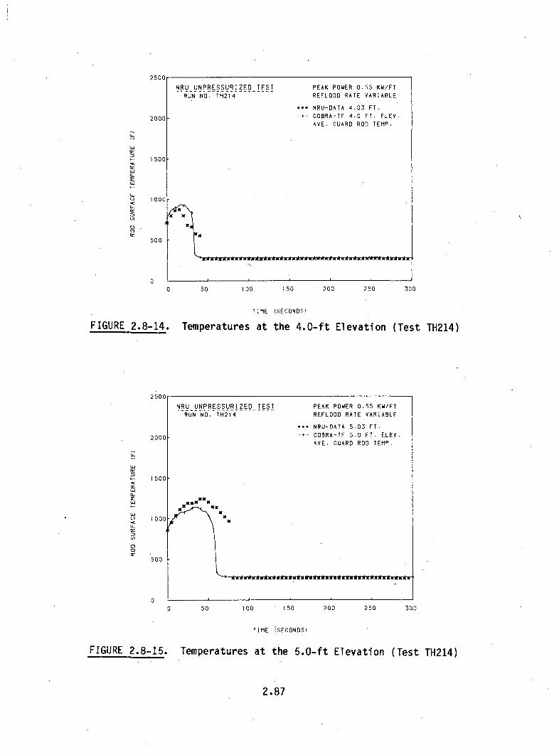
IL
IL
tIL
IL
I-)
IL
00 50 100 150 200 250 300
Ti1ME (SECONDS
Temperatures at the 4.0-ft Elevation (Test TH214)FIGURE 2.8-14.
CL
Ui
0
50 100 150 200 250 300
TIME (SECONDS)
FIGURE 2.8-15. Temperatures at the 5.0-ft Elevation (Test TH214)
2.87

NRU UNPRESSURIZED TEST,RU NO. H
PEAK POWER 0.55 KW/FTREFLOOD RATE VARIABLE
2000
E
LU.
Uj
0Or
1500
... NRU-DATA 6.36 FT.
"÷- COBRA-TF 6.0 FT. ELEV.
kVE. GUARD ROD TEMP.
XMIE 'K wx 'w~ m
N(X, W
l000
500
00 50 100 150 200 250 300
TIME (SECONDS)
FIGURE 2.8-16. Temperatures at the 6.0-ft Elevation (Test TH214)
ýq flC
NRU UNPRESSURIZED TESTRUN 61NO. -- TH-2-1 4
PEAK POWER 0.55 KW/FT
REFLOOD RATE VARIABLE
2000
U-A
U.'
Uj
(-
*.. NRU-DATA 6.4 - 8-. FT.COBRA-TF 7.0 FT. ELEV.AVE. GUARD ROD TEMP.
1500
500
00 50 100 150 200 250 300
TIME (SECONDS)
FIGURE 2.8-17. Temperatures at the 7-ft Elevation (Test TH214)
2.88

NRUUNPRESSURIZNO.TH2RUN NO. TH214
PEAK POWER 0.95 KW/FTREFLOOD RATE VARIABLE
2000ý
cr
0cr.
• NRU-DATA 8.il FT.COBRA-TF 8.0 FT. ELEV.AVE.' GUARD ROD TEMP.
I500ý
1005
500 F
a0 50 100 150 200 250 300
TIME (SECONDS)
FIGURE 2.8-18. Temperatures at the 8.0-ft Elevation (Test TH214)
NRU UNPRESSURIZED TESTRUN NO. TH214
PEAK POWER 0.55 KW/FT
REFLOOD RATE VARIABLE
2000C
UJtsJ0-
U-
. NRU-DATA 9.R6 FT.
COBRA-TF 10.0 FT. ELEV.
kVE. GUARD ROD TEMP.
1500F
IOOC
500 F
0
0 50 100 150 200 250
TIME (SECONDS)
FIGURE 2.8-19. Temperatures at the 10.0-ft Elevation (Test TH214)
2.89
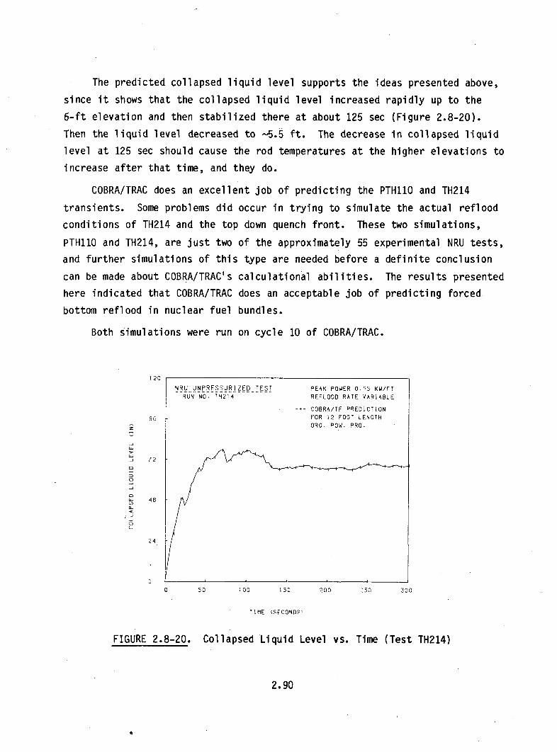
The predicted collapsed liquid level supports the ideas presented above,
since it shows that the collapsed liquid level increased rapidly up to the
6-ft elevation and then stabilized there at about 125 sec (Figure 2.8-20).
Then the liquid level decreased to -5.5 ft. The decrease in collapsed liquid
level at 125 sec should cause the rod temperatures at the higher elevations to
increase after that time, and they do.
COBRA/TRAC does an excellent job of predicting the PTH110 and TH214
transients. Some problems did occur in trying to simulate the actual reflood
conditions of TH214 and the top down quench front. These two simulations,
PTH110 and TH214, are just two of the approximately 55 experimental NRU tests,
and further simulations of this type are needed before a definite conclusion
can be made about COBRA/TRAC's calculational abilities. The results presented
here indicated that COBRA/TRAC does an acceptable job of predicting forced
bottom reflood in nuclear fuel bundles.
Both simulations were run on cycle 10 of COBRA/TRAC.
1 20
NRU UNPRESSURIZED TEST PEAK POWER O.S5 KW/FTRUN NO. TH214 REFLOOD RATE VARIABLE
-.- COBRA/TF PREDICTION96 FOR 12 FOOT LENGTH
ORG. POW. PRO.
. 72
0
48
02
0_24
0 0 100 150 200 .50 300
TIME kF(CONODS
FIGURE 2.8-20. Collapsed Liquid Level vs. Time (Test TH214)
2.90
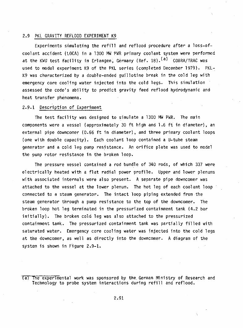
2.9 PKL GRAVITY REFLOOD EXPERIMENT K9
Experiments simulating the refill and reflood procedure after a loss-of-
coolant accident (LOCA) in a 1300 MW PWR primary coolant system were performed
at the KWU test facility in Erlangen, Germany (Ref. 18 ).(a) COBRA/TRAC was
used to model experiment K9 of the PKL series (completed December 1979). PKL-
K9 was characterized by a double-ended guillotine break in the cold leg with
emergency core cooling water injected into the cold legs. This simulation
assessed the code's ability to predict gravity feed reflood hydrodynamic and
heat transfer phenomena.
2.9.1 Description of Experiment
The test facility was designed to simulate a 1300 MW PWR. The main
components were a vessel (approximately 30 ft high and 1.6 ft in diameter), an
external pipe downcomer (0.66 ft in diameter), and three primary coolant loops
(one with double capacity). Each coolant loop contained a U-tube steam
generator and a cold leg pump resistance. An orifice plate was used to model
the pump rotor resistance in the broken loop.
The pressure vessel contained a rod bundle of 340 rods, of which 337 were
electrically heated with a flat radial power profile. Upper and lower plenums
with associated internals were also present. A separate pipe downcomer was
attached to the vessel at the lower plenum. The hot leg of each coolant loop
connected to a steam generator. The intact loop piping extended from the
steam generator through a pump resistance to the top of the downcomer. The
broken loop hot leg terminated in the pressurized containment tank (4.2 bar
initially). The broken cold leg was also attached to the pressurized
containment tank. The pressurized containment tank was partially filled with
saturated water. Emergency core cooling water was injected into the cold legs
at the downcomer, as well as directly into the downcomer. A diagram of the
system is shown in Figure 2.9-1.
(a) The experimental work was sponsored by the. German Ministry of Research andTechnology to probe system interactions during refill and reflood.
2.91
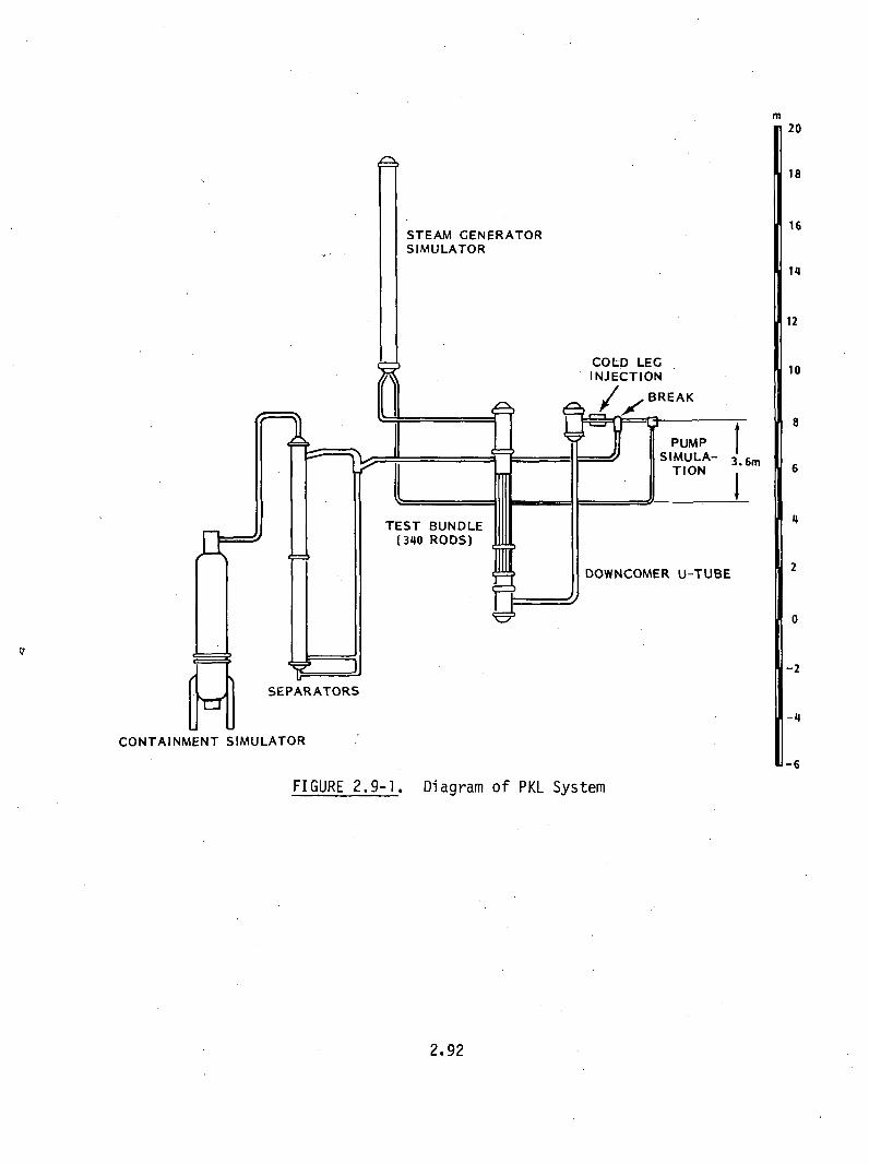
m
STEAM GENERATORSIMULATOR
COLD LEGINJECTION
BREAK
20
18
16
14
12
10
8
6
4
2
0
-2
-4
-6
TEST BUNDLE(340 RODS)
DOWNCOMER U-TUBE
SEPARATORS
CONTAINMENT SIMULATOR
FIGURE 2.9-I. Diagram of PKL System
2.92

2.9.2 COBRA/TRAC Model Description
A COBRA/TRAC system component schematic for PKL-K9 is illustrated in
Figure 2.9-2. The vessel and downcomer were modeled with the vessel component
(component 1). The hot and cold leg pipes and the steam generators were
simulated with the appropriate one-dimensional components.
A detailed diagram of the COBRA/TRAC model of the pressure vessel and
downcomer is shown in Figure 2.9-3. This part of the facility was modeled
with the three-dimensional vessel component. The vessel component contained
five vertical sections. Section one modeled the bottom half of the lower
plenum and the downcomer pipe connection. Section two modeled the top half of
the lower plenum and the corresponding piece of the downcomer. The core and
downcomer were simulated by sections three and four. Section five modeled the
upper plenum and the top of the downcomer. Fourteen channels in five sections
provided 82 mesh cells. One average heater rod, with a heated length of
12.67 ft located in core channels 3 and 4 (14.79 ft), was used to model the
337 heated rods in the core. A one-dimensional nodalization was used to
minimize computation time. The vertical node length was chosen to coincide
with measurement locations.
The three coolant loops of PKL-K9 were modeled with two equivalent loops
that consisted of the flow area of the three loops. The broken cold leg
(pipe 7) and the broken hot leg (pipe 4) were connected to break components 6
and 5 respectively. These break components modeled the containment pressure
history described in the PKL documents (Ref. 18, 19 and 20). The intact cold
leg (pipe 10), ECC injection, and broken cold leg (pipe 7) connect to the
downcomer at nodes 4, 5, and 6, as illustrated in Figure 2.9-3. This
configuration simulated the PKL-K9 test where ECC injection was into the
intact loop cold legs.
The initial conditions for fluid state and rod temperatures were obtained
from the PKL documents (Ref. 18,19). The vessel, the primary sides of the
steam generators, and all pipes were initially filled with saturated steam.
The secondary sides of the steam generators were filled with water to a height
of 7.5 m. Initial flows in the system were zero. The initial vessel pressure
was set to the specified pressure of 4.6 bars.
2.93

BR
#/COMPONENT NUMBERS
FIGURE 2.9-2. COBRA/TRAC Model of PKL Test Facility
BROKEN
UPPER
UPPER T
HOT LEG - -------
PLENUMI L ----AE - -- - --
IE PL AT -O-
CORE
LOWER TIE PLATE-)-
.4-
SBROKEN:..~COLD LEG
-•• ECC INJECTION
COLD LEGINTACT~
HOT -
LEG
DOWNCOMER
14 13LOWER PLENUM
1
FIGURE 2.9-3. Schematic of COBRA/TRAC Model of PKL Pressure Vessel andDowncomer
2.94
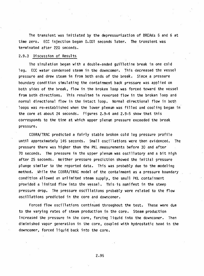
The transient was initiated by the depressurization of BREAKs 5 and 6 at
time zero. ECC injection began 0.001 seconds later. The transient was
terminated after 220 seconds.
2.9.3 Discussion of Results
The simulation began with a double-ended guillotine break in one cold
leg. ECC water condensed steam in the downcomer. This decreased the vessel
pressure and drew steam in from both ends of the break. Since a pressure
boundary condition simulating the containment back pressure was applied on
both sides of the break, flow in the broken loop was forced toward the vessel
from both directions. This resulted in reversed flow in the broken loop and
normal directional flow in the intact loop. Normal directional flow in both
loops was re-established when the lower plenum was filled and cooling began in
the core at about 24 seconds. Figures 2.9-4 and 2.9-5 show that this
corresponds to the time at which upper plenum pressure exceeded the break
pressure.
COBRA/TRAC predicted a fairly stable broken cold leg pressure profile
until approximately 145 seconds. Small oscillations were then evidenced. The
pressure there was higher than the PKL measurements before 30 and after
70 seconds. The pressure in the upper plenum was oscillatory and a bit high
after 25 seconds. Neither pressure prediction showed the initial pressure
plunge similar to the reported data. This was probably due to the modeling
method. While the COBRA/TRAC model of the containment as a pressure boundary
condition allowed an unlimited steam supply, the small PKL containment
provided a limited flow into the vessel. This is manifest in the steep
pressure drop. The pressure oscillations probably were related to the flow
oscillations predicted in the core and downcomer.
Forced flow oscillations continued throughout the test. These were due
to the varying rates of steam production in the core. Steam production
increased the pressure in the core, forcing liquid into the downcomer. Then
diminished vapor generation in the core, coupled with hydrostatic head in the
downcomer, forced liquid, back into the core.
2.95

500
400
w
z
w
ccC,,
0.
zwU-j(L
300
E EN
-H E
R
PKL DATA
COBRA-TRAC PREDICTION
I I I I I I _ _
200
100
UII
00 50 100 150 200 250 300TIME (seconds)
350
FIGURE 2.9-4. Pressure in the Upper Plenum (Channels 5-8)
500
400
LU
w
0.
Fw
3000.
"" PKL DATA
--- COBRA-TRAC PREDICTION
III I I I
200
100
0 0 50 100 150 200 250 300 350TIM E (seconds)
FIGURE 2.9-5. Pressure in the Break Pipe
2.96

Collapsed water level'measurements agreed well with the PKL reported data
(Figure 2.9-6) but following 150 seconds the water level appeared low.
The downcomer mass flow rate also oscillated. Figures 2.9-7 and 2.9-8
show downcomer flow rates in channel 10, the former averaged over the entire
channel while the latter was taken at the lower node boundary. (The PKL
measurement was at a similar location.) It appears that the COBRA/TRAC
prediction follows the correct trend.
Clad temperature profiles at several elevations in the core are shown in
Figures 2.9-9 through 2.9-15. Peak clad temperatures occur about 25 seconds
after the start of the transient. This was when the lower plenum was filled
with water and the bottom of the core was beginning reflood. Quench fronts
through level four (--6.4 ft) were well predicted by COBRA/TRAC. Above level 4
the code underpredicted the heat transfer associated with top down quenching
and consequently did not predict quench time at these elevations. A plot of
the quench front envelope is shown in Figure 2.9-16.
The void fractions, shown Figures 2.9-17 through 2.9-19, also
fluctuated. The severe oscillations may have been driven by the critical heat
flux switching logic. The damping effects of a turbine flow meter in the
power part of the downcomer possibly should have been modeled with a loss
coefficient.
In summary, COBRA/TRAC predicted the temperature profiles in PKL in the
lower half of the core well. It had difficulty with quench front in the core
upper half because it did not correctly predict the falling film heat
transfer. It is believed that the new top quench front model will improve
data comparisons in the upper half of the core. Upper plenum pressure, break
pressure and collapsed water level in the core predictions agreed fairly well
with the measured data. Something is awry in the void fraction and downcomer
velocity predictions. This simulation was run on cycle 10 of COBRA/TRAC.
2.97

10.
xI-
W-JF-0(
r0
0)
E
-J
-j
TIME(seconds)
FIGURE 2.9-6. Collapsed Water Level in the Core
WC,,
w
0
z
0
zI-
0-jU.
100
60
20
-20
-60
-1000 50 100 150 200 250 300 350
TIME (seconds)
FIGURE 2.9-7. Flow Rate in the Downcomer (Averaged Over Length of Channel 10)
2.98

c3U)
LUw
LU
o
(3
zLU0
k-
C._
zL
100
60
20
-20
-60
-1000 50 100 150 200 250 300 350
TIME (seconds)
FIGURE 2.9-8. Flow Rate in the Downcomer (at the Lower Boundary Node)
4 f rJfI JLU I
800
U-
D
0
ir
0
I-
LU
LI-
600
T/C 185
- PKL DATA LEVEL 1 (0.492 ft)
--- COBRA/TRAC PREDICTION
I I I I I I
400
200
j*'
0 50 100 150 200 250 300 350
TIME (seconds)
FIGURE 2.9-9. Rod Surface Temperature at Level 1
2.99
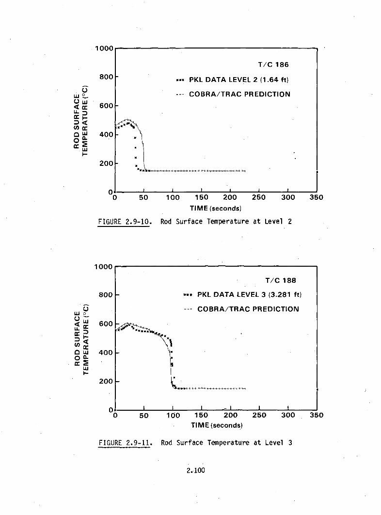
10 V,•.
800 F
LU
LL(n
0
LUcc
ILl
I-
600 -
T/C 186
• PKL DATA LEVEL 2 (1.64 ft)
COBRA/TRAC PREDICTION
I a I I
400
200
A I II I I I I I
I
0 50 100 150 200 250 300 350
TIME (seconds)
Rod Surface Temperature at Level 2FIGURE 2.9-10.
1000
800
UiwLA
C,,
0
0
LU
0.
LU
600
T/C 188
w=* PKL DATA LEVEL 3 (3.281 ft)
COBRA/TRAC PREDICTION
W I II-
400
200
IJ A - -
0 50 100 150 200 250 300 350TIME (seconds)
FIGURE 2.9-11. Rod Surface Temperature at Level 3
2.100

1000
800
00.
I--
600
T/C 191
* PKL DATA LEVEL 4 (6.398 ft)
--- COBRA/TRAC PREDICTION
S. ...........
400
200
n I |
0 50 100
FIGURE 2.9-12. Ro
1000r
150 200 250 300TIME (seconds)
d Surface Temperature at Level 4
350
800
wo
u.•
0 a.
I-
600
T/C 193
m PKL DATA LEVEL 42 (8.465 ft)
COBRA/TRAC PREDICTION
Mgm
I I tI l
400
200
1A0 0 50 100 150 200
TIME (seconds)
250 300 350
FIGURE 2.9-13. Rod Surface&'Temperature at Level 42
2.101

1000
(L
I-
LU
0X
800
600
400
200
JULY 20, 1981T/C 195
... PKL DATA LEVEL 51(10.335 FT.)
--- COBRA/TRAC
PREDICTION
'Il
I'
00 50 100 150 200 250 300 350
TIME (seconds)
w
IL
wu.I-w
C.
uJ.U--
LU
a0
xI:
FIG
1000
800
600
400
200
URE 2.9-14.
JULY 20, 1981
T/C 198
. PKL DATA LEVEL 7 (12.303 FT.)
COBRA/TRAC PREDICTION
INHmN - •W
Rod Surface Temperature at Level 51
1000 50 100 150 200 250 300 350
TIME (seconds)
FIGURE 2.9-15. Rod Surface Temperature at Level 7
2.102

PKL REFILL AND REFLOOD TEST K9
10
8
U--
z0
6
4
2
0
6.398 ft.LEVEL .4'
4.314 ft.LEVEL 33.28 ft.LEVEL 2
1.64 ft.LEVEL 1
0 50 100 150 200 250 300 350
TIMAE (SECONDS)
FIGURE 2.9-16. Quench Front Envelope
1.00
0.80
z01'- 0.60U
J.)LL
2 0.400
0.20
0.000 50 100 150 200 250 300 350
TIME (seconds)
FIGURE 2.9-17. Void Fraction in the Core, (Channel 3, Nodes 3-5)
2.103
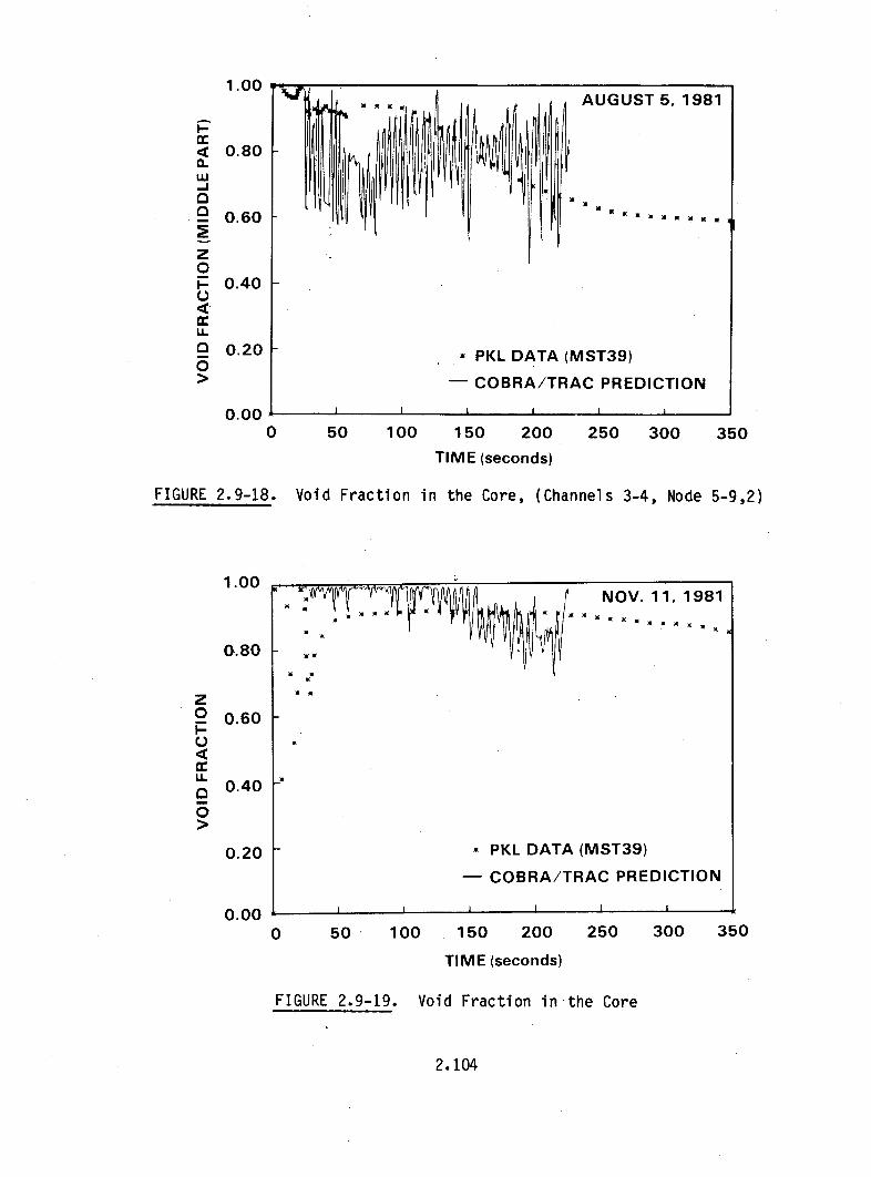
P
h-CL
0
z0
LL.
a0U-
1.00
0.80
0.60
0.40
0.20
0.000 50 100 150 200
TIME (seconds)
250 300 350
FIGURE 2.9-18. Void Fraction in the Core, (Channels 3-4, Node 5-9,2)
1.00
0.80
C.)
g0
0.60
0.40
0.20
0.000 50 100 150 200
TIME (seconds)
250 300 350
FIGURE 2.9-19. Void Fraction in the Core
2.104

2.10 CYLINDRICAL CORE TEST FACILITY GRAVITY REFLOOD EXPERIMENT C1-2
A COBRA/TRAC simulation of a gravity feed reflood experiment conducted in
the JAERI cylindrical core test facility (CCTF) (Ref. 21) was made to assess
the code's ability to predict gravity feed reflood transients. This
simulation tested the code's ability to predict the system transient response
and feedback to the thermal-hydraulic behavior of the core during reflood.
Steam binding caused by steam flow through the hot legs, steam generators and
pumps occurred in the test and was modeled in COBRA/TRAC. The effects of
evaporation of drops carried over from the core into the steam generators, de-
entrainment of liquid drops in the upper plenum, downcomer filling behavior,
and transient carryover and reflood in the core were also modeled.
2.10.1 Description of Experiment
The large-scale experiment CCTF test C1-2 (Run 011) was chosen for this
simulation. The CCTF was designed to model a full-height core section and the
intact and broken loops of a PWR. The facility contained a nonnuclear core of
2000 electrically heated fuel rod simulators arranged in a rectangular array
and placed within a cylindrical vessel. The test vessel included a downcomer,
lower plenum, core region and upper plenum with associated internals. The
intact loop represented the three intact loops of a PWR and included a steam
generator and pump simulator with associated piping.' The broken loop also
contained a steam generator and pump simulator. The test was initiated by
turning on the power to the core with the vessel filled with steam except for
0.86 m of saturated water in the lower plenum. The rods heated up virtually
adiabatically in the core's steam environment. Fifty-three seconds after
power was applied to the fuel rod simulators, accumulator injection into the
lower plenum was initiated. When the liquid level reached the bottom of the
core at 69 sec, the accumulator injection was switched to the cold leg for the
remainder of the transient. The core power decay was initiated at 67 sec. At
78 sec, accumulator injection ended and low pressure coolant injection (LPCI)
was initiated. All heater rods were quenched by 588' sec.
A schematic of the CCTF system is shown in Figure 2.10-1. The scaled
dimensions for the various components of the system are provided in
Table 2.8. The CCTF dimensions are compared to the dimensions of a PWR to
2.105

STEAM SUPPLY LINE
I
STEAMSUPPLY
ACC LINE CONTAINMENT TANK-I
FIGURE 2.10-1. Schematic of Cylindrical Core Test Facility

TABLE 2.8. Component Dimensions of Cylindrical Core Test Facility
COMPONENT PWR JAERI RATIO
PRESSURE VESSEL
Vessel Inside Diameter (mm) 4394 1084
Vessel Thickness (mm) 216 90
Core Barrel Outside Diameter (mm) 3874 961(mm) 3760 929
Thermal Shield Outside Diameter (mm) 4170Thermal Shield Inside Diameter (mm) 4030Downcomer Length (mm) 6066 6066 1/1Downcomer Gap (mm) 114.3 61.5Downcomer Flow Area (i 2 ) 4.23 0.197 1/21.44Lower Plenum Volume (m3 ) 29.6 1.38 1/21.44Upper Plenum Volume (m3 ) 43.6 2.04 1/21.44
FUEL (HEATER ROD) ASSEMBLYNumber of Bundles (--) 193 32Rod Array (--) 15 x 15 8 x 8Rod Heater Length (mm) 3660 3660 1/1Rod Pitch (mm) 14.3 14.3 1/1Fuel Rod Outside Diameter (mm) 10.72 10.7 1/1Thimble Tube Diameter (mm) 13.87 13.8 1/1Instrument Tube Diameter (mm) 13.87 13.8 1/1Number of Heater Rods (--) 39372 1824 1/21.58Number of Nonheating Rods (--) 4053 224 1/18.09Core Flow Area (M2) 5.29 0.25 1/21.2Core Fluid Volume (in) 7.95 0.813 1/21.2
PRIMARY LOOPHot Leg Inside Diameter (mm) 736.6 155.2 1/4.75Hot Leg Flow Area (m2 ) 0.426 0.019 1/22.54Hot Leg Length (mm) 3940 3940 1/1Pump Suction Inside Diameter (mm) 787.4 155.2 1/5.07
Pump Suction Flow Area (m2 ) 0.487 0.019 1/25.77Pump Suction Flow Length (mm) 7950 7950 1/1
2.107

give an idea of the modeling scale. The dimensions for the vessel are shown
in Figure 2.10-2. The configuration of the rods in the core are shown in
Figure 2.10-3. The core is divided into the three main power zones: low,
intermediate and high. The lower power zone consists of zones M2 through M4
shown in Figure 2.10-3. The intermediate power zone consists of zones M6
through M9, and M5 is the high power zone. The axial power profile is shown
in Figure 2.10-4 along with the locations of rod thermocouples. The test
conditions are summarized in Table 2.9.
2.10.2 COBRA/TRAC Model Description
A diagram of the COBRA/TRAC model of CCTF is shown in Figure 2.10-5. the
system was modeled with appropriate one-dimensional components for the intact
and broken loops, including steam generators.
The CCTF vessel was modeled using a one-dimensional representation of the
core, lower plenum, downcomer and upper plenum. A diagram of the vessel model
is shown in Figure 2.10-6. The flow paths through orifices, support columns
and guide tubes in the upper plenum were also modeled. Twelve 1-ft long nodes
were used in the core and downcomer. The heater rods were modeled using a
single average rod heat transfer model. The thermal capacitance of the vessel
and core barrel wall were modeled with heat slabs to obtain the effects of hot
walls on downcomer penetration. The pump flow resistances were modeled by
specifying a constant loss coefficient at the appropriate locations in the
loop piping. ECC water injection was modeled using fill components in the
cold leg piping. The containment was modeled by specifying a constant
pressure at the end of the broken cold leg and hot leg piping.
2.10.3 Discussion of Results
An oscillatory reflood behavior was computed throughout the test. The
period of the oscillation was on the order of 2 sec. The amplitude of the
oscillation was largest at the initiation of reflood and diminished as the
transient proceeded.
Comparisons between predictions and the experimental data are shown in
Figures 2.10-7 through 2.10-19. Figures 2.10-7 through 2.10-14 show
2.108
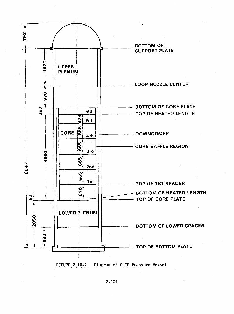
BOTTOM OFSUPPORT PLATE
LOOP NOZZLE CENTER
BOTTOM OF CORE PLATE
- TOP OF HEATED LENGTHL
L DOWNCOMER
CORE BAFFLE REGION
d
TOP OF 1ST SPACER
BOTTOM OF HEATED LENGTHTOP OF CORE PLATE
M
BOTTOM OF LOWER SPACER
s -L TOP OF BOTTOM PLATE
Diagram of CCTF Pressure VesselFIGURE 2.10-2.
2.109

SYMBOLS
• HIGH POWER HEATER ROD[ MEDIUM POWER HEATER FF] LOW POWER HEATER ROD
NON-HEATING ROD
FIGURE 2.10-3.
NAME OF POWER ZONES
Cross Section of CCTF Core
2.110

3.5
3.0
2.5
z04.
U.IwU
2.0
1.5
MIDPLANE
1.0
0.5
0
0
w w w~,,I- I- I-
U Uw 4
(--JLMo ()
0 0.5 1.0 1.5AXIAL POWER PROFILE (Q/QAv)
FIGURE 2.10-4. Axial Power Profile and Thermocouple Elevations for HeaterRods in CCTF Core
2.111

TABLE 2.9. Summary of Conditions for CCTF Test (1-2)
1. TEST TYPE: TEST C1-2 (CCTF MAIN TEST NO. 20)2. TEST NUMBER: RUN 011 3. DATE: July 4, 19794. POWER: A: TOTAL: 9.36 MW; B:LINEAR: 1.4 KW/M5. RELATIVE RADIAL POW:R7 PE
A: ZONE: A B CB: RATIO: 1.07 : 1.0 : 0.82
6. AXIAL POWER SHAPE: CHOPPED COSINE7. PRESSURE (KG/CM 2 a):
A: SYSTEM: 2.07* , B: CONTAINMENT 2.06C: STEAM GENRTOR SCONDARY: 50
8. TEMPERATURE (DEG.C):A: DOWNCOMER WALLS 187 , B: VESSEL INTERNALS 120C: PRIMARY PIPING ALL'118 D: LOWER PLENUM LI0UTITE: ECC LIQUID 39 , F: STEAM GENERATOR SECID'A- 263G: CORE TEMPERTUR AT ECC INITIATION 506
9. ECC INJECTION TYPE: CA: COLD LEG, B: LOWER PLENUM, C: LOWER PLENUM + COLD LEG
10. PUMP K-FACTOR: -15 (UNCERTAIN)11. ECC FLOW RATFS AND DURATION:
A: ACCUMULATOR 264 Ma/HR FROM 0 TO 25 SECONDSB: LPCI 9 M3 /HR FROM2Srdr7 SECONDSC: ECC INJLCTI1F n LOWER PLEI -- FROM0T-- TO 16 SECONDS
(VALVE OPENING AND CLOSING TIMES ARE TTUDJU'rT-FrHE INJECTIONDURATION)
12. INITIAL WATER LEVEL IN LOWER PLENUM: 0.86 M.13. POWER CONTROL: ANS x 1.2 + ACTINIDE (-•--F C AFTER SCRAM)14. EXPECTED BOCREC TIME FROM ECC INITIATION 12 SEC15. EXPECTED PEAK TEMPERATURE AT BOCREC 600 T7
* Since system pressure drops below containment pressure in initial stages ofECC injection, condensation in the vessel was set to zero when this occurredto simulate air intake from containment.
2.112

PIPE
O JUNCTION
ED COMPONENT NUMBER
FIGURE 2.10-5. Schematic of COBRA/TRAC Model of CCTF
GUIDE TUBES
AND ORIFICESSUPPORT COLUMN
AND STUBS
DOWNCOMER
4
2
.. .. j I- '.---
13 13 1 14 1 I 14-- --- I--- L-
- I I _- ----- 16---
s
2~
UPPER PLENUM
UPPER TIE PLATE
CORE
LOWER CORESUPPORT PLATE REGION
LOWER PLENUM
1 CHANNEL NUMBERS
FIGURE 2.10-6. Vessel Mesh for CCTF
2.113

0.020
o. 0.016
ci 0.012LU
0.008z
LL 0.004
E5
0 000 0 00 0
0 CCTF DATA
COBRA/TRAC PREDICTION
0.000 I I I
0 100 200 300
TIME (sec)
400 500 600
FIGURE 2.10-7.
0.01 I-
Differential Pressure in the Lower Plenum
(U
cr
U)LU
-J
zUJ
UJU.
0.008
0.006
0.004
0.002
0.000 100 200 300 400 500 600
TIME (seconds)
FIGURE 2.10-8. Differential Pressure Between the 0 and 2-ft Elevations in theCore
2.114

0U
LU
cc
z
LUL-
0.01
0.008
0.006
0.004
0.002
0.00
0 100 200 300TIME (sec)
400 500 600
FIGURE 2.10-9. Differential Pressure Between 2Core
and 4-ft Elevations in the
0U
cc
Ch
5z
0Ucc
U.U-
a
0.01
0.008
0.006
0.004
0.002
0.00
0 100 200 300 400 500 600
TIME (seconds)
FIGURE 2.10-10. Differentialin the Core
Pressure Between the 4 and 6-ft Elevations
2.115
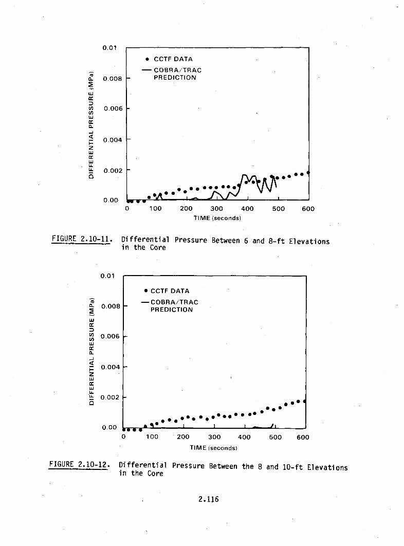
0.01
0.0080.
-JUi
zUJ
U-
LL
0 .006 I-
* CCTF DATA
COBRA/TRACPREDICTION
0 .0 @0000 • .
oo 0O 0 ••
0.004
0.002 -
0.00 _ • -- __ a m ! Im i i
0 100 200 300 400
TIME (seconds)
500 600
FIGURE 2.10-11. Differential Pressure Between 6 andin the Core
8-ft Elevations
0.01
CL
wLU
Cn
U,
0--J
n-z
U-LL
* CCTF DATA
- COBRA/TRACPREDICTION0.008 h
0.006
0.004
0.002 k0 4
00.000
* ~. 000000
* 00*00 0 000
0.00 I - I aI
0 W W 100 200 300 400 500 600
TIME (seconds)
FIGURE 2.10-12. Differential Pressure Between the 8 and 10-ft Elevationsin the Core
2.116
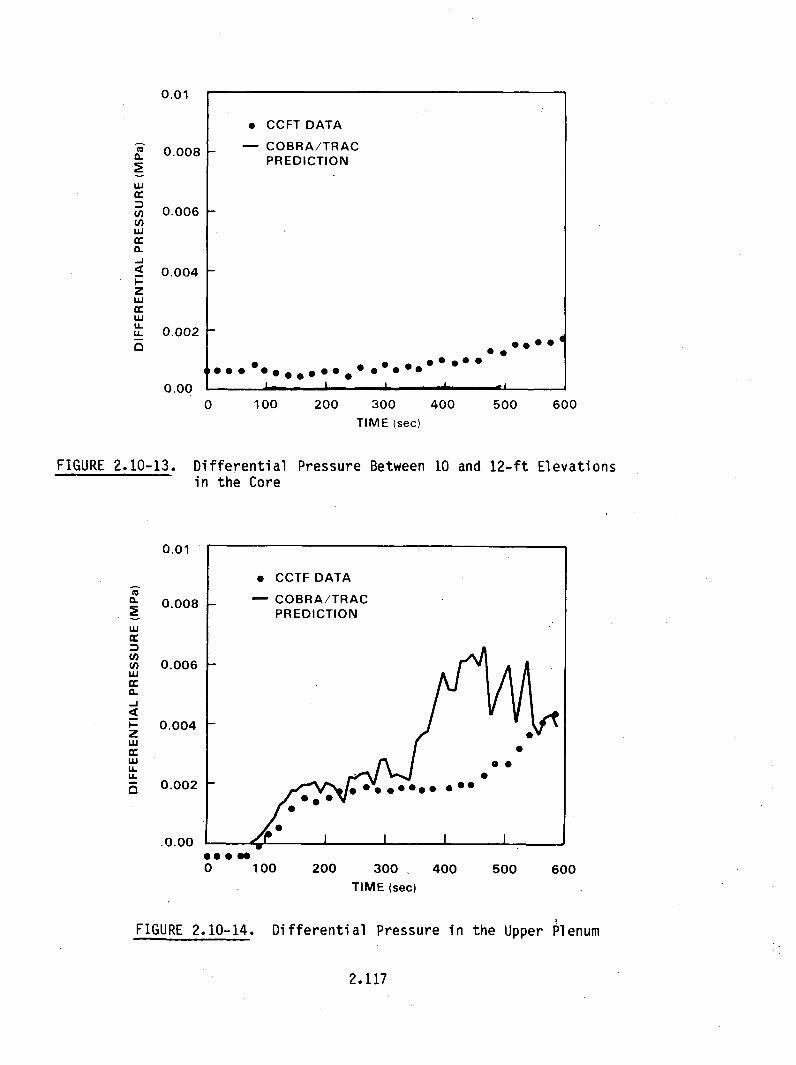
0.01
CL
0.
U)
LU
zW
LU
U-
0.008
0.006
0.004
0.002
o CCFT DATA
COBRA/TRACPREDICTION
0000
1000 0 00000000 0 00 000 00 00 0'-- . • I g
0.000 100 200 300 400
TIME (sec)
500 600
FIGURE 2.10-13. Differential Pressure Betweenin the Core
10 and 12-ft Elevations
0.01
(L
a-
U).U
w0~
F-
W
z
wU.U-
0.008
0.006
0.004
0.002
'0.00.**o.
0 100 200 300
TIME (sec)400 500 600
FIGURE 2.10-14. Differential Pressure in the Upper Plenum
2.117
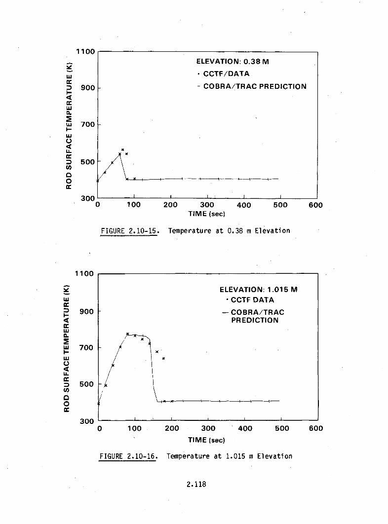
1100
2
,Ui
I--
U.
0
I-
U)4LL
900
ELEVATION: 0.38 M
CCTF/DATA
- COBRA/TRAC PREDICTION
700
500
300'0
I I I I I
100 200 300TIME (sec)
400 500 600
FIGURE 2.10-15. Temperature at 0.38 m Elevation
1100
9
LU
I-
4<€
I--
LU
L.
00
ELEVATION: 1.015 M
• CCTF DATA
COBRA/TRACPREDICTION
900
700
500
3000 100 200 300 400 500
TIME (sec)
600
FIGURE 2.10-16. Temperature at 1.015 m Elevation
2.118
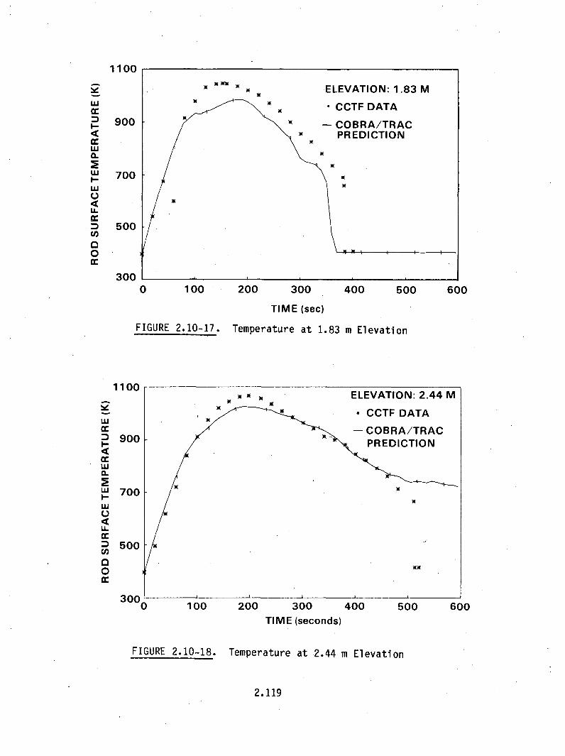
1100
ELEVATION: 1.83 M
CCTF DATA
900 g- COBRA/TRAC- PREDICTION
wU.
0.
c c 7 0 0 1
C-)U-
S500
0
3 0 0,,,,,
0 100 200 300 400 500 600
TIME (sec)
FIGURE 2.10-17. Temperature at 1.83 m Elevation
1100 1 1 ELEVATION: 2.44 M,,,E •/•• • •CCTF DATA
- COBRA/TRAC
900 PREDICTIONc-w0.
W 700
w
D 500
a x0
0 100 200 300 400 500 600
TIME (seconds)
FIGURE 2.10-18. Temperature at 2.44 m Elevation
2.119

1100
9ELEVATION: 3.05 Mw - CCTF DATA
D 900 - COBRA/TRACI- PREDICTION
w 700w /.U-
• 500
C,,0
3000 100 200 300 400 500 600
TIME (sec)
FIGURE 2.10-19. Temperature at 3.05 m Elevation
comparisons of predicted differential pressures in the lower plenum, core and
upper plenum. (Comparisons with downcomer differential pressures are not
shown. These data were used to obtain a corrected ECC injection rate since
discussion with other investigators indicated that the reported values may be
in error. The temperature of the injected water was also uncertain since
there appears to have been segments of piping filled with saturated water
between the ECC water supply and the simulated reactor vessel. This caused a
significant period of saturated water injection into the vessel before
subcooled water actually reached it. The fill rates and temperatures were
corrected to account for these uncertainties. The flows were corrected based
on the downcomer filling rate, so any comparison between the code predictions
of the downcomer liquid level (AP) and the measured data would be, of
necessity, very good.)
Differential pressures for the lower plenum are shown in Figure 2.10-7.
The prediction is slightly higher than the data due to the difference in
location between the pressure taps and computational mesh cell centers.
Otherwise, the comparison is very good and indicates that the lower plenum
filled at the right time and at about the right rate.
2.120

Comparisons of differential pressures (void fractions) in the core are
shown in Figures 2.10-8 through 2.10-13. The comparisons below 6 ft are all
good, indicating that the interfacial shear and vapor generation models are
predicting about the right void fraction in the core. The computed liquid
level is much more oscillatory than the data indicates. The oscillation has a
period of about 2 sec. The plotting interval used to generate Figure 2.10-8
was too large (10 sec) to show theocorrect period for the oscillation, but the
general magnitude is about right. Very large oscillations occur shortly after
water first enters the core. The magnitude diminishes later on in the
transient. It is uncertain whether oscillations of such magnitude actually
occurred in the test and the measurement system was not able to detect them,
or if heat transfer or flow regime transitions in COBRA/TRAC are responsible
for generating them. It is likely that the answer is somewhere in between.
Work is in progress to understand exactly what the driving mechanism for the
oscillations are, to see if they are physical or numerical.
The differential pressure in the top portions of the core indicate that
COBRA/TRAC may be under-predicting the liquid content of the flow in the
core. The differential pressures for the upper plenum are shown in
Figure 2.10-14. The liquid level in the upper plenum is well predicted out to
about 320 sec. At that point a sudden increase in the differential pressure
is predicted that is not seen in the data. Part of this increase is caused by
the liquid level reaching and submerging the hot leg outlets. The remainder
is caused by excessive carryover from the core. This comparison indicates
that the liquid carryover and de-entrainment in the upper plenum were
correctly predicted during the first 320 sec of the transient.
Heater rod surface temperature comparisons are shown for five elevations
in the core in Figures 2.10-15 through 2.10-19. Predictions at the four lower
elevations are very good both on-peak clad temperature and quench time. The
peak temperatures are slightly underpredicted at the middle two elevations.
This may be the result of excessively large flow oscillations. The peak clad
temperature of the highest elevation, shown in Figure 2.10-19, is predicted
but the turnaround time is overpredicted and the rod is cooling too slowly.
This is probably a result of the underprediction of the liquid content of the
.flow at this elevation.
2.121

2.11 NORTHWESTERN UNIVERSITY COUNTERCURRENT FLOW FILM CONDENSATION EXPERIMENT
This simulation analyzed the steam-water countercurrent condensation
tests (Ref. 22) in a vertical test section at Northwestern University. The
experimental tests investigated the condensation rates for countercurrent flow
in a vertical channel approximately 3/20th the size of a nuclear reactor
downcomer. The simulations of the Northwestern experiment were initiated to
assess the interfacial heat transfer and drag coefficient equations used for
countercurrent film flow.
2.11.1 Description of Experiment
The major components of the test facility (test section, upper and lower
plenums) were designed and constructed of aluminum and transparent
polycarbonate. A diagram of the test section and adjoining entrance and exit
plenums is shown in Figure 2.11-1. The test section dimensions were 3.81 cm
wide, 38.1 cm deep, and 96.5 cm high. The upper plenum consisted of a water
inlet plenum designed to form a liquid film on the test section wall and a
steam exit plenum. The steam entrance and water exit plenums were
incorporated into a lower plenum. The design of the steam entrance plenum
assured a uniform flow distribution.
There were six steam flow measurement stations within the test
facility. They were located in the inlet and outlet steam feed tubes and at
30.48-cm intervals within the active portion of the test section starting
2.54 cm above the lower plenum connection flange. The steam flow rates were
measured using a steam venturi for the measurements outside the test section
and with heated pitot tubes within the test section. The water flow rates
were measured only at the entrance and exit of the test facility by means of
flow meters. The inlet and exit temperatures of both the steam and water were
also measured.
The tests were performed from set initial flow conditions at a pressure
of 1 atmosphere and with the test section tilted 7 degrees from vertical. The
test section was tilted to reduce the effects produced by flow down the edges
of the flow channel. Forty-nine tests were run varying the steam flow from
0.074 to 0.084 kg/s, the water flow from 0.80 to 1.78 kg/s, and the
2.122

STEAM OUT*
WATER IN
50 IN.TESTSECTION
MEASUREMSTATIONS
FIGURE 2.11-1. VerCoI
STEAM IN
tical Test Apparatus for Countercurrent Flow Filmndensation Experiments
2.123

temperature of the incoming water from 35 to 710C. An attempt was made to
keep the inlet steam temperature constant throughout the test series but it
also varied from 129.9 to 141.6 0 C.
Prior to each test the test section was preheated with steam flow. After
preheating, a steady two-phase flow was established throughout the test
section. This was accomplished by adjusting the water flow and temperature to
the desired values for a given run and then adjusting the steam flow rate and
temperature to their prescribed values. Once a steady-state condition was
established, ten 20-sec steam flow data scans were performed over the 3.30 cm
steam flow width. Upon completion of the data scans, a computer compiled and
calculated the integrated mass flow rate for each pitot tube, the average
steam and water temperatures at the entrance and exit locations. The local
heat transfer coefficient at the pitot tube locations was also computed from
the measured data.
2.11.2 COBRA/TRAC Model Description
Figure 2.11-2 shows a detailed noding diagram for this problem. The
system was modeled using 7 components and 6 junctions. The vessel component
contained two channels with 3 and 11 fluid nodes in the lower and upper
channels. The lower channel was added only as a water accumulation plenum and
did not exist on the actual test section. The steam and water were injected
by FILLS 1 and 3 into the simulated test section at the appropriate
elevations. The steam exited through PIPE 6, which was connected to the top
of the second vessel channel. A water flow boundary condition was imposed at
the bottom of channel one to drain away the excess water accumulation if
necessary. A one-dimensional nodalization was used in this simulation to test
the film flow correlations within a mesh cell.
The entire test system, except for the water fill and pipe, was
initialized to the inlet steam conditions for experimental test case no. 1..
The water and pipe fill were initialized at their respective values. At time
zero both the steam and water flow were initiated and the system achieved a
steady-state condition after about 2.5 sec. Condensation was set to zero in
the three lower channel nodes. This was done because in the actual experiment
these water accumulation nodes did not exist.
2.124

STEAMBREAK-- I1ýPRESSURE
BOUNDARY
WATERFILL
FLOWE*~*l i~irE A OiJ
® COMPONENTS
XF ] JUNCTIONS
50oin.VESSEL
STEAM
~ FILL
FLOWBOUNDARY
ZERO FLOWBOUNDARY
FIGURE 2.11-2. COBRA/TRAC Model for NWU CCFF Condensation Tests
2.125
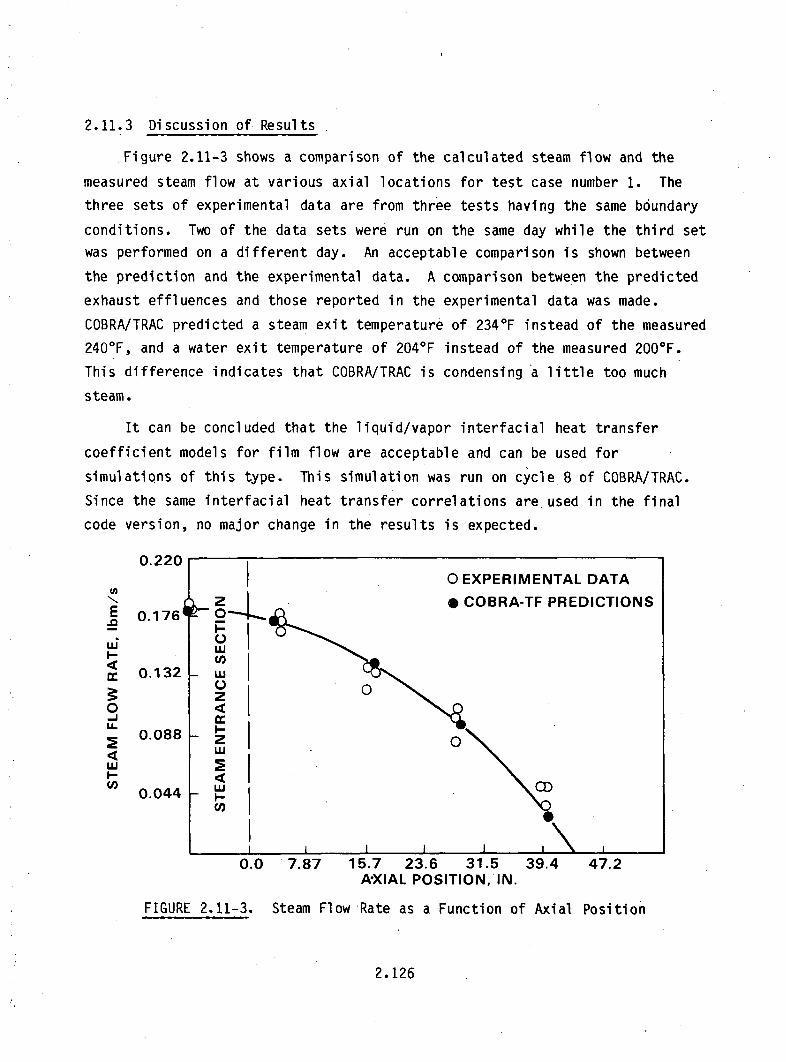
2.11.3 Discussion of Results
.Figure 2.11-3 shows a comparison of the calculated steam flow and the
measured steam flow at various axial locations for test case number 1. The
three sets of experimental data are from three tests having the same boundary
conditions. Two of the data sets were run on the same day while the third setwas performed on a different day. An acceptable comparison is shown between
the prediction and the experimental data. A comparison between the predicted
exhaust effluences and those reported in the experimental data was made.
COBRA/TRAC predicted a steam exit temperature of 234°F instead of the measured
240 0 F, and a water exit temperature of 204 0 F instead of the measured 2000 F.
This difference indicates that COBRA/TRAC is condensing a little too much
steam.
It can be concluded that the liquid/vapor interfacial heat transfer
coefficient models for film flow are acceptable and can be used for
simulations of this type. This simulation was run on cycle 8 of COBRA/TRAC.
Since the same interfacial heat transfer correlations are used in the final
code version, no major change in the results is expected.
0.2200 EXPERIMENTAL DATA
z 9" COBRA-TF PREDICTIONSE 0.176
IdL III1i
r~0.132 w
0.00.088 - 0w0
0.044 - uCD
~ I 0
0.0 7.87 15.7 23.6 31.5 39.4 47.2A#XIAL POSITION, IN.
FIGURE 2.11-3. Steam Flow Rate as a Function of Axial Position
2.126

2.12 RPI FLAT PLATE PHASE DISTRIBUTION EXPERIMENT
Simulations have been run for two experiments in the Rensselear
Polytechnic Institute (RPI) phase separation series (Ref. 23). The purpose of
these simulations was to test the ability of the code, with a three-
dimensional turbulence model, to predict the void distribution in a
recirculating two-dimensional, two-phase flow.
One of the most difficult aspects of a multidimensional turbulent two-
phase flow to predict accurately is the phase distribution. Experiments
(Ref. 24,25) have shown that the dispersed phase tends to migrate to regions
of high continuous-phase turbulent intensity. It has been theorized (Ref. 26)
that the turbulent normal stresses are primarily responsible for this
behavior. Thus, it appears that any code used for phase distribution
predictions needs a reasonable turbulence model.
The turbulence model currently available in COBRA/TRAC is a three-
dimensional mixing length model. The mixing length is variable and parametric
values must be supplied by the user. Both-the turbulent (Reynolds) stresses
and the turbulent heat flux are included in the model, as well as the.viscous
shear stresses.
2.12.1 Description of Experiment
The experimental apparatus, shown in Figure 2.12-1, consisted of a two-
dimensional thermoplastic test section, measuring 1/2 in. x 12 in. x 36 in.
An air-water mixture was injected at the bottom and withdrawn from outlets
near the top. Steady-state tests were conducted with various flowrates and
inlet qualities. Runs were made both with and without 24 simulated fuel rods
of 1/4 in. diameter and 1/2 in. pitch. In addition, the mass withdrawal
method was varied: in some cases all mass was removed from one side of the
test section; in others it was equally split between the two horizontal
outlets. The local void fraction was measured 'at 20 locations in the test
section using a gamma densitometer system.
2.127
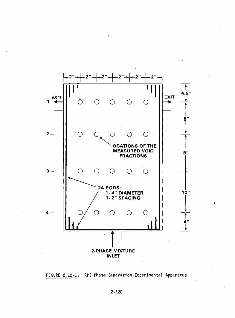
Ir- ý"
II I II IEXIT1 4-
2-
3-
4-
EXIT0 0 0 0 0
0 0 1Q 0 0 0
LOCATIONS OF THEMEASURED VOID
FRACTIONS
4.5"
8"
9,,
0 0 0
24
0 0
DIAMETERSPACING
R11
OD./4"/22"
14),,
0 0 0 0
II P' III 4"
-L-2-HSIXTR
2-PHASE MIXTUREINLET
FIGURE 2.12-1. RPI Phase Separation Experimental Apparatus
2. 128

Two of the symmetric runs with rods in were chosen for initial
simulation. These runs had the same inlet quality but different flow rates.
RPI Test # 8:A = 206.53 Ibm/min, x = 0.257%
RPI Test # 10: m = 318.82 Ibm/min, x = 0.257%
The quality 0.257 corresponds to an inlet void fraction of approximately 0.6.
2.12.2 COBRA/TRAC Model Description
The COBRA/TRAC model is shown in Figure 2.12-2. Since the experiments
being simulated were symmetric, only half of the test section was modeled.
The vessel component, a short PIPE and a BREAK were used. The vessel mesh was
comprised of 12 levels with five cells on each level for a total of
60 computational cells. This mesh was chosen to minimize the number of mesh
cells while providing sufficient resolution of velocity and void profiles
necessary for the computation of the turbulent shear stresses.
The air and water mixture was simulated using saturated steam and water
at 40.7 psia. At this pressure the gas/liquid density ratio is the same as in
the actual experiment. Boundary conditions for the simulations were flow and
enthalpy at the inlet and pressure at the break. Each simulation was run as a
transient from a standing start with initially no vapor in the test section.
The mass flow rate was ramped from zero to its full value in 0.2 sec and the
transient continued until the change in the dependent variables was
sufficiently small to indicate that a steady state had been achieved.
2.12.3 Discussion of Results
Simulation results for the steady-state void fraction distribution are
presented in Figures 2.12-3 through 2.12-6. Void profiles are shown for the
four axial locations where data were taken. The solid curves give the
experimental results and the dashed lines are the code prediction.
Figures 2.12-3 and 2.12-4 show results obtained without using the turbulence
model while Figures 2.12-5 and 2.12-6 depict the same simulations with the
turbulence model.
Figure 2.12-3 shows results from RPI test #8, which had the lower flow
rate. The experimental results clearly show the affinity of the vapor phase
2.129

1 1PLANE OF2 - SYMMETRY
INLET
0 4 ®®®FIGURE 2.12-2. COBRA/TRAC Model of the RPI Phase Separation Experiment Test
Section
2.130
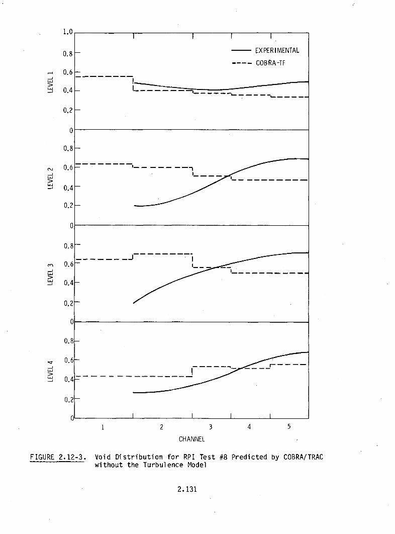
12 3 4 5
CHANNEL
Void Distribution for RPI Test #8 Predicted by COBRA/TRACwithout the Turbulence Model
FIGURE 2.12-3.
2.131

1.0 I
0.8 EXPERIMENTAL
COBRA-TF0.6
LU-~-
__- 0.4 I__
0.2
0
0.8
0.6.-J
LU
__ 0.4
0.2
0
-I0.8 -...
evn 0.6
-j 0.4
0.2
0
0.8 I
'IT 0.6LU
LU
0.4
0.2
1 2 3 4 5
CHANNEL
FIGURE 2.12-4. Void Distribution for RPI Test #10 Predicted by COBRA/TRACwithout the Turbulence Model
2.132

.J,,J
LJ-j
CJ
L.J
LUJ-j
1.0
0.8
0.6
0.4
0.2
0
0.8
0.6
0.4
0.2
0
0.8
0.6
0.4
0.2
0
0.8
0.6
0.4
0.2
0
.- J
LUlLU
_J
._J
12 3 4 5
CHANNEL
FIGURE 2.12-5. Void Distribution forthe Turbulence Model
RPI Test #8 Predicted by COBRA/TRAC with
2.133

1.0
0.8
0.6
0.4
- EXPERIMENTAL
COB RA-TF
*1
LUI-,J
0.2H
0
.-J
-,J__j
0.8
0.6
0.4
--------
0.2h
0
0.8 H
_-J
Uj-j
0.6
0.4 ..........................
0.2H
0
0.81-
_.JLIU
-J
0.6"
0.4
0.21-
I I
1 2 3 4 5
CHANNEL
FIGURE 2.12-6. Void Distribution for RPI Test #10 Predicted by COBRA/TRACwith the Turbulence Model
2.134

for the highly turbulent region near the jet centerline. At level 4, near the
bottom of the test section, the computed results show the correct trend, but
the profile is more uniform than the experimental profile. The prediction is
worse at levels 2 and 3 where the computed solution shows too much vapor on
the left side of the test section and not enough on the jet axis. The
prediction at level 1, near the top of the test section, is fairly good,
although the values near the jet centerline should be higher.
COBRA/TRAC results for test #10, which has the higher flowrate, are shown
in Figure 2.12-4. The experimental results show slightly flatter void
profiles than in test #8, but the trend toward maximum void fraction at the
jet centerline is still obvious. The code prediction without turbulence
modeling shows just the opposite t~rend, greatly overpredicting the amount of
vapor on the outlet side of the test section.
Figure 2.12-5 shows the code prediction with the turbulence model for
test #8. The turbulence model has improved the results significantly,
especially at levels 1, 3 and 4. Even at level 2, where the prediction is not
quite as good, the code at least predicts the correct trend toward maximum
void fraction at the jet centerline. This simulation was performed using a
mixing length of 0.25 in. in channels 1 through 4, and a value of 0.5 in. in
channel 5. Trials with a single constant value of 0.3 in. gave similar
results, but the prediction at levels 1 and 2 was not as good.
Code predictions for test #10 with turbulence are given in Figure 2.12-6
which shows results obtained for a constant mixing length of 0.33 in.
Comparison of Figure 2.12-6 with Figure 2.12-4 shows a marked improvement at
all axial levels when turbulence is used.
The steady state was attained after three seconds of transient time for
all runs. The execution speeds and average time step sizes for the four runs
are given in Table 2.10.
In summary, COBRA/TRAC uses a three-dimensional turbulence model based on
mixing length theory. The simulations presented above indicate that the model
can significantly improve calculations where detailed phase distribution
information is desired and reasonably fine noding is justified. Although the
2.135

TABLE 2.10. Execution Speeds and Average Time Steps for Calculations of RPIPhase Separation Tests
Execution Speed Average Time StepRUN (sec/At-cell) (sec/At)
RPI-8 (no turbulence) 3.90(10)- 3 6.06(10)-3
RPI-10 (no turbulence) 3.86(10)- 3 4.38(10)-3
RPI-8 (with turbulence) 4.04(10)- 3 5.57(10)-3
RPI-10 (with turbulence) 3.97(10)- 3 3.95(1o)-3
model can easily accommodate a spatially varying mixing length, the results
given in this report were obtained using a constant value for the entire test
section, except near the jet axis. It is reasonable to assume that additional
experimentation with a variable mixing length could further improve the
calculation. This simulation was run on cycle 10 of COBRA/TRAC.
2.13 BENNETT TUBE CRITICAL HEAT FLUX EXPERIMENTS
Experiments investigating dryout and post-CHF heat transfer (Ref. 27)
were simulated to assess the code's ability to calculate both the dryout point
and heat transfer to dispersed flow beyond the dryout point. (The dryout
point is defined as the axial location where liquid is no longer in contact
with the tube wall.) Since heat transfer to a vapor droplet mixture is much
lower than heat transfer to continuous liquid, the dryout point can be
identified by a sharp increase in wall temperature. COBRA/TRAC's calculation
of liquid film dryout is compared to the dryout point measured in the Bennett
Tests (indicated by a sharp increase in wall temperature) and to the dryout
point predicted by the Biasi CHF correlation.
2.13.1 Description of Experiment
The Bennett Tests were a series of experiments carried out in the Harwell
High Pressure Two Phase Heat Transfer Loop. The main objectives of the tests
were to measure surface temperature profiles in the region beyond the dryout
point and to investigate the behavior of the dryout interface.
2.136

An electrically heated Nimonic alloy tube served as the test section.
The tube was 0.497 in. I.D., 0.625 in. O.D., and 19 ft long, Nimonic alloy
was used because of its low temperature coefficient of electrical resistivity,
which provided a nearly uniform heat flux with large axial temperature
variation. The tube geometry eliminated the problems encountered with spacers
and offered a more straightforward means of comparison with theoretical
model s.
To prepare for each test the system was brought to the specified pressure
(nominally 1000 psia) and inlet temperature with the test section power just
below that required for CHF. The power was then increased until the top-most
thermocouple showed a rapid increase in temperature, indicating CHF.
Conditions were allowed to reach steady state. The temperatures, power, flow
and exit pressure were recorded by a data logging system. The power was again
increased until the next thermocouple exhibited a rapid increase in
temperature. The readings were taken again. This procedure was repeated
until the maximum temperature of the rod approached 14000 F. Power was then
decreased and readings made as each successive thermocouple exhibited a rapid
decrease in temperature.
2.13.2 COBRA/TRAC Model Description
A simple COBRA/TRAC model was used to simulate the Harwell Loop for this
series of experiments. The model consisted of a PIPE, a BREAK and a VESSEL
component. A diagram of the model is shown in Figure 2.13-1.
The vessel component modeled the test section of the Harwell Loop. The
vessel consisted of 20 cells in three vertically connected channels.
Channels 1 and 2, each containing nine 1-ft long cells, modeled the heated
length. A rod of tube geometry with heat transfer to the fluid on the inside
surface simulated the heated Nimonic tube. Properties of the Nimonic 80A
alloy used in the simulation do not change with temperature. Material
properties were not important in this simulation since the tests were at
steady state and the only parameter of interest was the wall surface
temperature. A uniform power profile was used in both the axial and radial
directions. Channel 3 of the vessel, with two 1-ft cells, provided the exit
length and was connected to the pipe component.
2.137
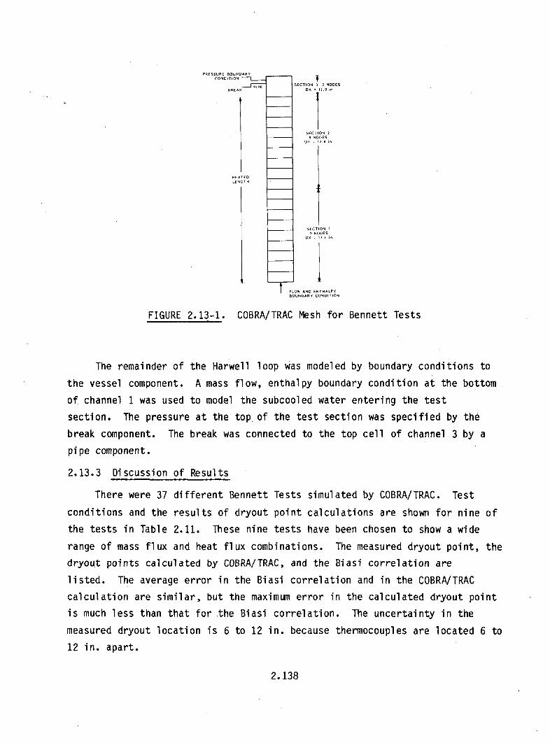
PRESSURE BOUNDARYCONDITION
BREAK
HEATEDLENGTH
SECTION 3 2 NODESDX ý 12 .0 i
SECTION 29 NODES
SECTION II NODES
DO - 12.0 m,
FLOW AND ENTRALPYBOUNDARY CONDITION
FIGURE 2.13-1. COBRA/TRAC Mesh for Bennett Tests
The remainder of the Harwell loop was modeled by boundary conditions to
the vessel component. A mass flow, enthalpy boundary condition at the bottom
of channel 1 was used to model the subcooled water entering the test
section. The pressure at the top of the test section was specified by the
break component. The break was connected to the top cell of channel 3 by a
pipe component.
2.13.3 Discussion of Results
There were 37 different Bennett Tests simulated by COBRA/TRAC. Test
conditions and the results of dryout point calculations are shown for nine of
the tests in Table 2.11. These nine tests have been chosen to show a wide
range of mass flux and heat flux combinations. The measured dryout point, the
dryout points calculated by COBRA/TRAC, and the Biasi correlation are
listed. The average error in the Biasi correlation and in the COBRA/TRAC
calculation are similar, but the maximum error in the calculated dryout point
is much less than that for the Biasi correlation. The uncertainty in the
measured dryout location is 6 to 12 in. because thermocouples are located 6 to
12 in. apart.
2.138

TABLE 2.11. Summary of Bennett TestCal cul ations
Conditions and Results of Dryout Point
Test
5359
5336
5273
5250
5294
5313
5310
5379
5397
Mass Fl u(Ml b/hr-ft)
0.29
0.49
0.75
1.00
1.44
1.87
1.88
2.80
3.82
Heat Flux(MBtu/hr- ft2)
0.173
0.260
0.292
0.290
0.348
0.381
0.358
0.542
0.584
DryoutLocation
(in)
140
140
140
164
164
170
185
140
164
Avg error =
Max error =
Error (AZ)Biasi COBRA-IF
-20 - 8
-44 - 8
- 8 +26
+ 4 +16
+ 4 +16
+10 +10
+19 + 7
- 8 +16
-24 + 4
15.7 12.3
44 26
COBRA/TRAC uses the Biasi correlation for CHF when the mass flux is
greater than 30 gm/cm2 -sec and the flow regime is not annular film flow. In
the Bennett tests the liquid does form an annular film on the tube surface.
Instead of limiting the heat flux by the Biasi correlation, COBRA/TRAC uses
forced convection to the liquid film until the film is completely vaporized or
entrained. The results shown in Table 2.11 indicate that the film dryout
approach is an improvement over the Biasi correlation, at least for film
dryout CHF.
The entrainment rate is important in determining dryout of a liquid
film. COBRA/TRAC uses separate models for entrainment and de-entrainment that
result in a net entrainment rate. Figure 2.13-2 shows the effect of
entrainment on film dryout in test no. 5373. The entrained liquid fraction
increases rapidly at 6 to 8 ft from the bottom of the heated length indicating
a large positive entrainment rate. The entrainment rate decreases gradually
as the entrained liquid becomes a large fraction of the total liquid mass from
2.139

4 f•
.u TOTAL LIQUID
E 0.8-•••A&'-=•A0. A AAA A
wj AS0.6-
A
0.j 0.4 A--- ENTRAINED LIQUIDU.
40.2-
0 A I I I II I I
4 6 8 10 12 14 16 18 20 22AXIAL LOCATION (ft)
FIGURE 2.13-2. Entrained Liquid in Bennett Test No. 5373
8 to 12 ft. From 13 ft to the dryout point at 16 ft, continuous liquid has
become a small fraction of the total liquid mass flow. The de-entrainment
rate is larger than the entrainment rate and liquid droplets are deposited on
the liquid film.. Net de-entrainment near the dryout point of the annular film
is typical of all the Bennett Tests.
The COBRA/TRAC calculation of CHF is compared with the Biasi correlation
and the Bennett Test measurements as a function of equilibrium quality at the
dryout point in Figures 2.13-3 through 2.13-6. In each figure, measured data,
COBRA/TRAC calculations and a line representing the Biasi correlation are
plotted for a series of tests at a single mass flux.
Equilibrium quality for each of the Bennett experiments was calculated as
fol lows:
2.140
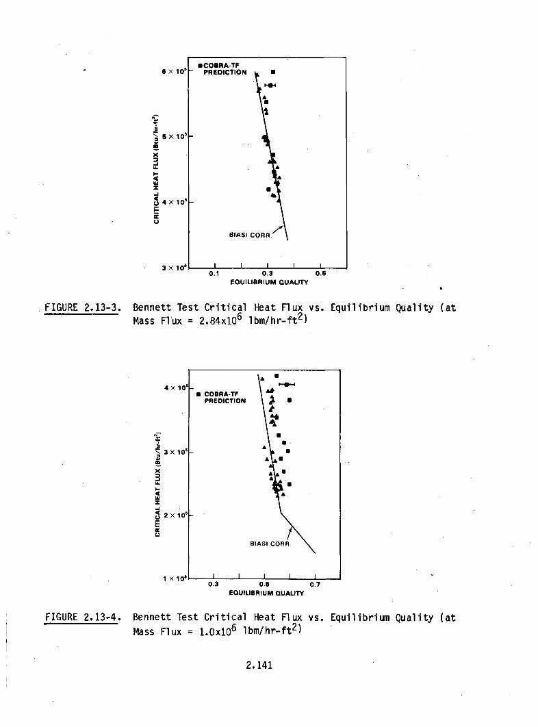
6 X 10⁵
U.,-SX 0Z
Xh3
U.
3 X 10⁵
5
•COBRA-TF- PREDICTION a
A
A
A
BIASI COR R.:'A
I I I I IV -
0.1 0.3EQUILIBRIUM QUALITY
0.5
FIGURE 2.13-3. Bennett Test CriticalMass Flux = 2.84x10⁶
Heat Flux vs. Equilibrium Quality (at1 bm/hr-ft
2 )
U
4 X 10'
3 3X 10'
UL.
I 2X10³
a COBRA-TF -PREDICTION
A'
A
A
BIASI CORR.
0.3 0.5EQUILIBRIUM QUALITY
0.7
FIGURE 2.13-4. Bennett Test Critical Heat Flux
Mass Flux = 1.0x10⁶ lbm/hr-ft 2 )vs. Equilibrium Quality (at
2.141

4 X 10,
0 COBRA-TF PREDICTION
a
J3X 105
X
U. ALX
.4
-.j 2 X 10⁵
* A
,41
BIASI COARR
lX 10 1 I 1 1 10.5 0.7 0.9
EQUILIBRIUM QUALITY
FIGURE 2.13-5. Bennett Test Critical Heat Flux vs. Equilibrium Quality atMass Flux = 0.49x10 6 lbm/hr-ft 2 )
II CORA-TF PREDICTION
~2X10 I I
X 4l
R*AA A A
L.
1X 10⁵
U
BIASI CORR.
0.7 0.8 0.9 1.0EQUILIBRIUM QUALITY
FIGURE 2.13-6. Bennett Test Critical Heat Flux vs. Equilibrium Quality (atMass Flux = 0.29xj0 6 lbm/hr-ft 2 )
2.142

mvao =q"Pw LX = v w (2.5)eq mtotal mtotal Ah
where Xeq = equilibrium quality at the dryout point
m vapor= vapor mass flow rate at the dryout point (lb/hr)
mtotal = total mass flow rate (lb/hr)
q"= heat flux (Btu/hr-ft 2 )
Pw= wetted perimeter of the tube (ft)
L = distance from bottom of heated length to dryout point (ft)
Ah= change in enthalpy from test section inlet to saturated steam
at dryout point (Btu/lb)
This equation is valid since the test section is at steady state and the
heat flux is uniform over the length of the tube. The largest uncertainty in
the equation is the location of the dryout point. In this analysis, dryout is
assumed to occur halfway between the thermocouple indicating a sharp increase
in temperature and the thermocouple immediately below it. Most dryout points
occur at or above 140 in. from the bottom of the heated length in a region of
the test section where thermocouples are less than 6 in. apart so that the
uncertainty in equilibrium quality is less than 5%.
The COBRA/TRAC quality is simply the mass flow rate of vapor divided by
the total mass flow rate at the dryout point. The dryout point is defined as
halfway between the first axial node in dispersed flow film boiling and the
axial node immediately below it. Dryout, therefore, always occurs at a cell
boundary. The mass flow rates from the fluid cells above and below were
linearly averaged to get mass flow at the cell boundary. The uncertainty due
to the axial node size was indicated on each of the four plots by an error bar
on one of the calculated data points.
According to Biasi, CHF is a function of mass flux, pressure, hydraulic
diameter and quality. A discontinuity in slope is present in the Biasi
correlation prediction because the correlation uses the maximum of two
equations. One equation is for low quality and the other for high quality
CHF. The Biasi correlation is described in detail in Volume 1, Section 4.2 of
the COBRA/TRAC manual.
2.143
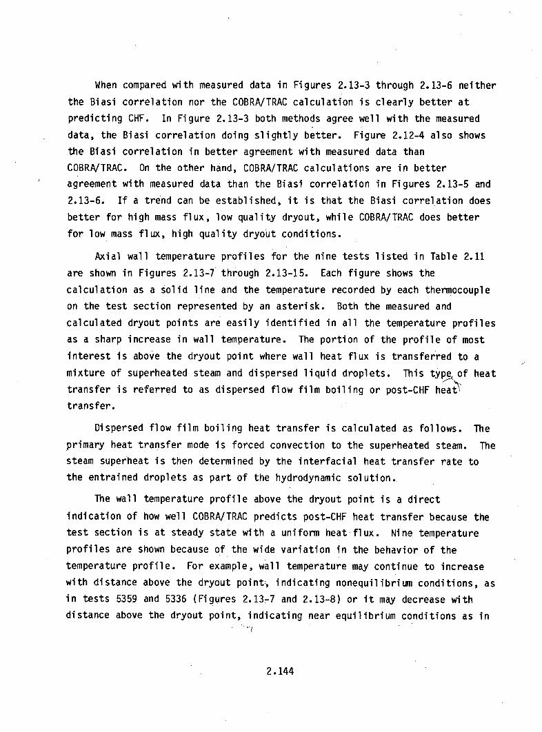
When compared with measured data in Figures 2.13-3 through 2.13-6 neither
the Biasi correlation nor the COBRA/TRAC calculation is clearly better at
predicting CHF. In Figure 2.13-3 both methods agree well with the measured
data, the Biasi correlation doing slightly better. Figure 2.12-4 also shows
the Biasi correlation in better agreement with measured data than
COBRA/TRAC. On the other hand, COBRA/TRAC calculations are in better
agreement with measured data than the Biasi correlation in Figures 2.13-5 and
2.13-6. If a trend can be established, it is that the Biasi correlation does
better for high mass flux, low quality dryout, while COBRA/TRAC does better
for low mass flux, high quality dryout conditions.
Axial wall temperature profiles for the nine tests listed in Table 2.11
are shown in Figures 2.13-7 through 2.13-15. Each figure shows the
calculation as a solid line and the temperature recorded by each thermocouple
on the test section represented by an asterisk. Both the measured and
calculated dryout points are easily identified in all the temperature profiles
as a sharp increase in wall temperature. The portion of the profile of most
interest is above the dryout point where wall heat flux is transferred to a
mixture of superheated steam and dispersed liquid droplets. This typeeof heat
transfer is referred to as dispersed flow film boiling or post-CHF heat•
transfer.
Dispersed flow film boiling heat transfer is calculated as follows. The
primary heat transfer mode is forced convection to the superheated steam. The
steam superheat is then determined by the interfacial heat transfer rate to
the entrained droplets as part of the hydrodynamic solution.
The wall temperature profile above the dryout point is a direct
indication of how well COBRA/TRAC predicts post-CHF heat transfer because the
test section is at steady state with a uniform heat flux. Nine temperature
profiles are shown because of the wide variation in the behavior of the
temperature profile. For example, wall temperature may continue to increase
with distance above the dryout point, indicating nonequilibrium conditions, as
in tests 5359 and 5336 (Figures 2.13-7 and 2.13-8) or it may decrease with
distance above the dryout point, indicating near equilibrium conditions as in
2.144

zw0.z
4
4
216
180
144
108
72
36
0
300
FIGURE 2.13-7
500 700 900 1100 1300 1500
WALL TEMPERATURE (DEG F)
Bennett Test 5359 Axial Temperatu'
1700
re Profile
a
z
z
4
216
180
144
108
72
•DATAS COBRA/TRAC PREDICTION
36
A
300 500 700 900 1100 1300 1500- 1700
WALL TEMPERATURE (DEG F)
FIGURE 2.13-8. Bennett Test 5336 Axial Temperature Profile
2.145
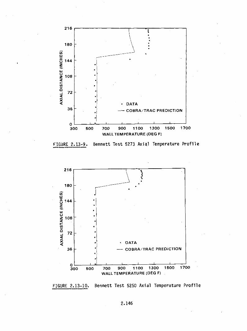
216
180
w5i
o 144z
wUz 108
4
_j 72
4
36
300 5'
FIGURE 2.13-9.
0D) 700 900 1100 1300 1500 1700WALL TEMPERATURE (DEG F)
Bennett Test 5273 Axial Temperature Profile
216
180
w
.144z
z 108I--
. 72
4x
36
01300 500 700 900 1100 1300 1500
WALL TEMPERATURE (DEG F)
1700
FIGURE 2.13-10. Bennett Test 5250 Axial Temperature Profile
2.146

216
180
U)
o 144z
L)Z 108
03
• 72
4
36
0300 5
FIGURE 2.13-11.
0(0 700 900 1100 1300 1500 1700WALL TEMPERATURE (DEG F)
Bennett Test 5294 Axial Temperature Profile
216
180
LU03X 144
zUj
z 108
I-U)
- 72
36
0300 500 700 900 1100 1300 1500' 1700
WALL TEMPERATURE (DEG F)
FIGURE 2.13-12. Bennett Test 5313 Axial Temperature Profile
2.147
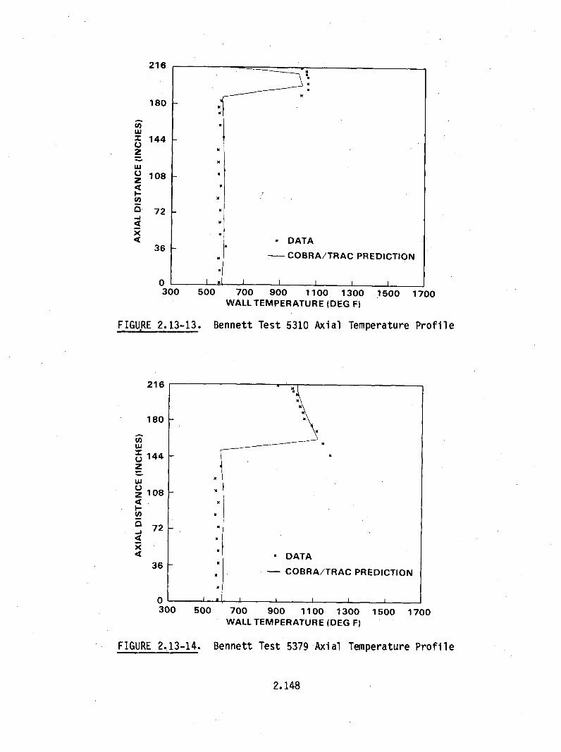
216
180
w
X 144U
IU
( 108z
72.--
• 72 K
X K - DATA36K 6 - COBRA/TRAC PREDICTION
0 I300 500 700 900 1100 1300 1500 1700
WALL TEMPERATURE (DEG F)
FIGURE 2.13-13. Bennett Test 5310 Axial Temperature Profile
216 -
180
uJ
144 K
z
wKz 108
O 72 "
x< DATA
36 K3 • COBRA/TRAC PREDICTION
0 I I 1300 500 700 900 1100 1300 1500 1700
WALL TEMPERATURE (DEG F)
FIGURE 2,13-14. Bennett Test 5379 Axial Temperature Profile
2.148

216
180
u 144Z
LU,4.L)
I,-
72
DATA36- 3- COBRA/TRAC PREDICTION
0 -300 500 700 900 1100 1300 1500 1700
WALL TEMPERATURE (DEG F)
FIGURE 2.13-15. Bennett Test 5397 Axial Temperature Profile
tests 5379 and 5397 (Figures 2.13-14 and 2.13-15). The wall temperature may
increase and then decrease as in tests 5250, 5294, and 5313 (Figures 2.13-10,
2.13-11 and 2.13-12) or remain relatively constant as in test 5273 and 5310
(Figures 2.13-9 and 2.13-13). Generally, COBRA/TRAC calculates wall
temperatures that are too low and decrease too much with axial distance from
the dryout point, except for tests 5379 and 5397. The maximum difference
between measured and calculated post-dryout wall temperature is 220 0 F in
test 5273. The behavior that COBRA/TRAC has the most trouble simulating is
increasing and then decreasing temperature above the dryout point. The code
completely misses the increasing part of the profile and predicts a
temperature gradually decreasing with distance above the dryout point.
The post-CHF wall temperature is dependent on vapor superheat.
Superheat, in turn, is a function of the dryout point, droplet size, slip
velocity and the interfacial heat transfer correlation. The fact that
calculated wall temperatures are too low and decrease too rapidly indicates
that an excessive amount of interfacial heat transfer is leading to a low
vapor temperature. Similar results have been noted in the upper elevations of
2.149

the FLECHT reflood tests with low flooding rate. COBRA/TRAC simulation of the
Bennett Tests has shown that the film dryout approach is an improvement over
the Biasi correlation for predicting the dryout location when annular film
flow is present. Using forced convection to the liquid film and not limiting
heat flux to the CHF calculated by the Biasi correlation has reduced the
average error and significantly reduced the maximum error in calculating
dryout location. Plotting CHF as a function of equilibrium quality has shown
that the calculation is sometimes better and sometimes inferior to the Biasi
correlation. A clear choice cannot be made as to which method predicts the
dryout equilibrium quality more reliably.
The Bennett test simulations also have shown that post-dryout heat
transfer is a difficult process to model. Wide variation in the behavior of
the wall temperature profiles indicate that some refinement of the dispersed
flow film boiling heat transfer regime is required to reduce uncertainty in
the calculated wall temperature profile.
2.150
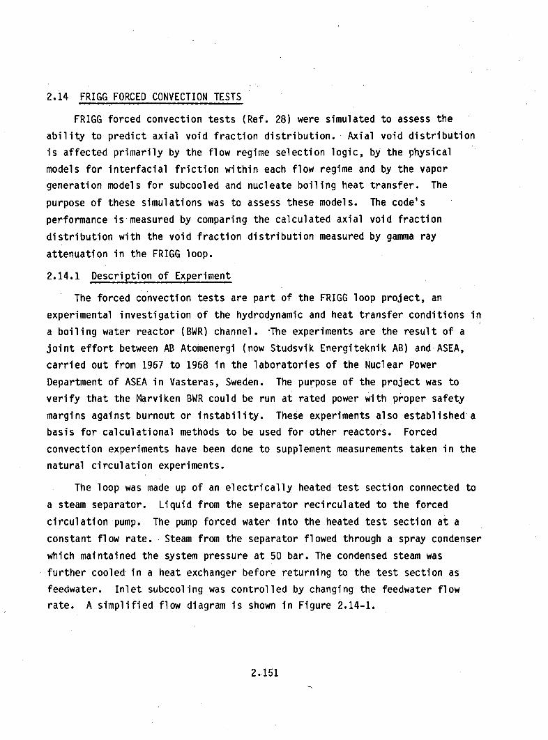
2.14 FRIGG FORCED CONVECTION TESTS
FRIGG forced convection tests (Ref. 28) were simulated to assess the
ability to predict axial void fraction distribution. Axial void distribution
is affected primarily by the flow regime selection logic, by the physical
models for interfacial friction within each flow regime and by the vapor
generation models for subcooled and nucleate boiling heat transfer. The
purpose of these simulations was to assess these models. The code's
performance is measured by comparing the calculated axial void fraction
distribution with the void fraction distribution measured by gamma ray
attenuation in the FRIGG loop.
2.14.1 Description of Experiment
The forced convection tests are part of the FRIGG loop project, an
experimental investigation of the hydrodynamic and heat transfer conditions in
a boiling water reactor (BWR) channel. -The experiments are the result of a
joint effort between AB Atomenergi (now Studsvik Energiteknik AB) and ASEA,
carried out from 1967 to 1968 in the laboratories of the Nuclear Power
Department of ASEA in Vasteras, Sweden. The purpose of the project was to
verify that the Marviken BWR could be run at rated power with proper safety
margins against burnout or instability. These experiments also established a
basis for calculational methods to be used for other reactors. Forced
convection experiments have been done to supplement measurements taken in the
natural circulation experiments.
The loop was made up of an electrically heated test section connected to
a steam separator. Liquid from the separator recirculated to the forced
circulation pump. The pump forced water into the heated test section at a
constant flow rate. Steam from the separator flowed through a spray condenser
which maintained the system pressure at 50 bar. The condensed steam was
further cooled in a heat exchanger before returning to the test section as
feedwater. Inlet subcooling was controlled by changing the feedwater flow
rate. A simplified flow diagram is shown in Figure 2.14-1.
2.151

FIGURE 2.14-1. Simplified Diagram of FRIGG Forced Convection Loop
The test section consisted of a uniformly heated 36-rod cluster with a
4.4-m heated length. The heater rod diameter was 13.8-mm and an unheated
center rod of 20 mm outer diameter was present. Prototypic reactor grid
spacers were used.
A gamma ray attenuation device measured the void fraction in the test
section. The device was mounted on an elevator to measure void fraction as a
function of axial level. The standard error of the measurements was 2.5%.
2.14.2 COBRA/TRAC Model Description
The COBRA/TRAC model for the forced circulation FRIGG loop consisted of
three components: a vessel, a pipe and a break. The vessel contained two
vertical channels with 14 fluid nodes. A schematic diagram of the model is
shown in Figure 2.14-2. A one-dimensional mesh was used and code predictions
are compared to the bundle average void fraction at each axial level.
Forced circulation flow into the bottom of the heated length was provided
by a vessel boundary condition. The boundary condition specified the enthalpy
and mass flow rate of water into the first node of the vessel. Section 1 of
2.152

BREAK __-TS 2.00' SECTI(
I 13 2 NOD
12
11
10
9
VESSEL 8
7 14.35' SECTI(12 NOI
6
5
4
3
2
MASS FLOW, ENTHALPYBOUNDARY CONDITION
)N 2ES
)N 1DES
FIGURE 2.14-2. COBRA/TRAC Model of FRIGG Forced Convection Loop
the vessel modeled the heated length of the test section. The fluid nodes
were thermally connected to an average rod simulating the 36 heater rods.
Loss coefficients were used to model the eight grid spacers in eight of the
fluid nodes of section 1. Section 2 of the vessel modeled the area of the
test section above the heated length. At the top of the section a pipe
connected the vessel to a break component. The break component modeled the
pressure boundary condition imposed on the test section by the remainder of
the FRIGG loop.
2.14.3 Discussion of Results
Test conditions of the FRIGG forced circulation tests simulated by
COBRA/TRAC are summarized in Table 2.12. The tests are identified by numbers
313020, 313018 and 313016. (These are code numbers of the steady state void
distribution measurements reported in Appendix 1 of the FRIGG loop project
documentation.) Inlet subcooling, inlet mass velocity, and total power were
experimentally measured. The COBRA/TRAC input parameters in Table 2.12 are
calculated from the measured quantities.
2.153

TABLE 2.12. Summary of FRIGG Forced Circulation Test Conditions
Test Number
313020 313018 313016
Inlet Subcooling (°C) 22.4 3.7 19.3
*Inlet Enthalpy (Btu/lbm) 448.34 487.92 454.71
Inlet Mass Velocity (kg/m 2 -sec) 1159 1124 1208
*Inlet Mass Flow rate (lbm/sec) 36.81 35.70 38.37
Total Power (kW) 4415 4390 2910
*Linear Heat Rate (kW/ft) 8.544 8.495 5.631
*Denotes parameters used in COBRA/TRAC input
A comparison of calculated and measured axial void distribution for each
of the FRIGG runs simulated is shown in Figures 2.14-3, 2.14-4 and 2.14-5.
The difference between measured and calculated void fraction is less than 5%.
In test 313018, liquid enters the test section only 3.7 0C subcooled.
According to COBRA/TRAC calculations, subcooled boiling takes place only in
the first node of the heated length. Vapor generation in the remainder of the
test section is due to nucleate boiling. Assuming that the subcooled boiling
model provides reliable results for the first node, agreement between
calculated and measured void distribution indicates proper calculation of the
flow regime and interfacial drag forces. Figure 2.14-3 shows how well the
calculated and measured axial void distribution agree.
In test 313020, the inlet subcooling is increased to 22.4 0 C. COBRA/TRAC
calculates a transition from subcooled to nucleate boiling seven feet from the
bottom of the heated length. The plot of void fraction as a function of axial
distance in Figure 2.14-4 shows a rapid increase of void fraction with axial
distance at the seven-foot level. This simulation indicates that the
subcooled boiling model combined with the subcooled liquid interfacial heat
transfer model, flow regime map, and interfacial shear models accurately
predict the void fractions in a boiling channel.
2.154

16
LL0
Oz
LL aW WUIz4
4W
12
8
4
MASS FLUX: 1124 Kg/sec M 2
EXIT QUALITY: 15.6
SUBCOOLING: 3.7 DEG C
HEAT FLUX: 64.3 W/cm2
- DATA
-COBRA-TF PREDICTION
n0.00 0.20 0.40 0.60 0.80
CHANNEL AVERAGE VOID FRACTION
1.00
FIGURE 2.14-3. FRIGG Forced Convection Test 313018
16
U-0
0
0
0
U-
x
C.)
o4
5-
zw
wx-
12
8
4
MASS FLUX; 1159 Kg/sec M 2
EXIT QUALITY: 9.6
SUBCOOLING: 22.4 DEG C
HEAT FLUX: 64.6 W/cm 2
DATA
- COBRA-TF PREDICTIONI I II
u0.00 0.20 0.40 0.60 0.80
CHANNEL AVERAGE VOID FRACTION1.00
FIGURE 2.14-4. FRIGG Forced Convection Test 313020
2.155
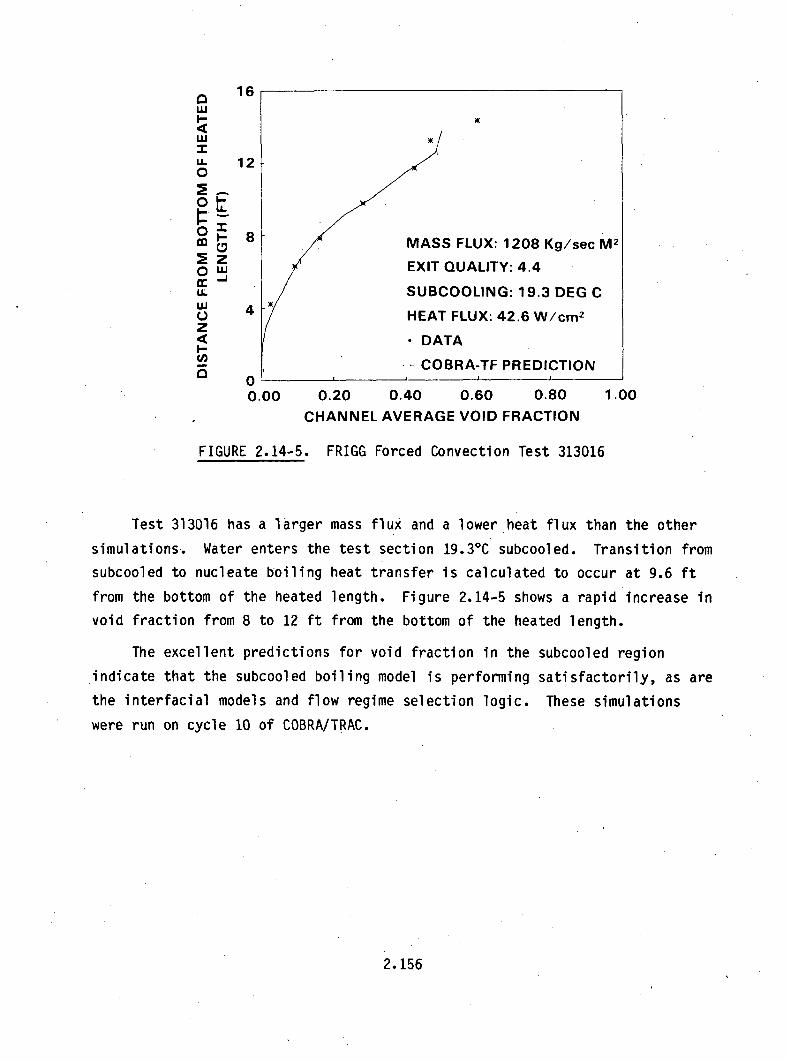
16
02
LL
LLUz
12
zU.
I-
)K
A
MAS!
EXIT
SUBC
HEAT
D r)SIA
4
S FLUX: 1208 Kg/sec M 2
E UALITY: 4.4
S OOLING: 19.3 DEG C
FLUX: 42.6 W/cm 2
[A
BRA-TF PREDICTION.- COl
0000.00 0.20 0.40 0.60 0.80
CHANNEL AVERAGE VOID FRACTION
1.1
FIGURE 2.14-5. FRIGG Forced Convection Test 313016
Test 313016 has a larger mass flux and a lower heat flux than the other
simulations. Water enters the test section 19.3 0C subcooled. Transition from
subcooled to nucleate boiling heat transfer is calculated to occur at 9.6 ft
from the bottom of the heated length. Figure 2.14-5 shows a rapid increase in
void fraction from 8 to 12 ft from the bottom of the heated length.
The excellent predictions for void fraction in the subcooled region
indicate that the subcooled boiling model is performing satisfactorily, as are
the interfacial models and flow regime selection logic. These simulations
were run on cycle 10 of COBRA/TRAC.
2.156

2.15 FRIGG NATURAL CIRCULATION TESTS
COBRA/TRAC simulations of FRIGG (Ref. 28) natural circulation experiments
have been done to assess the code's ability to calculate axial void
distribution in the heated length, two-phase flow pressure drop and the
natural circulation flow rate. The calculated axial void distribution is
compared to the void distribution measured by gamma ray attentuation.
COBRA/TRAC's calculation of two-phase flow pressure drop is assessed by
comparing measured and calculated inlet flow rate as a function of rod
power. In natural circulation the inlet flow rate is determined by the force
balance between the driving head in the downcomer and pressure losses in the
heated length. Hydrostatic and single-phase pressure losses are well
understood and have been tested in other simulations. Comparing the measured
and calculated inlet flow rate determines the credibility of the two-phase
flow pressure drop models used in COBRA/TRAC.
2.15.1 Description of Experiment
The FRIGG Loop project is an experimental investigation of hydrodynamic
and heat transfer conditions in a boiling water reactor (BWR) channel. The
experiments are the result of a joint project between AB Atomenergi and ASEA,
carried out from 1967 to 1968 in the ASEA laboratories in Vasteras, Sweden.
The purpose of the project was to establish a basis for calculational methods
to verify that BWR's can be operated at rated power with proper safety margins
against burnout or instability.
The loop is made up of an electrically heated rod bundle connected to a
steam separator. Liquid from the separator recirculates through the downcomer
to the bottom of the rod bundle. Steam from the separator is condensed in a
spray condenser and cooled in a heat exchanger before returning to the top of
the downcomer as feedwater. Inlet subcooling is controlled by the loop heat
exchanger. The loop pressure of 50 bar is maintained by the spray
condenser. Water from the downcomer flows into the heated length by natural
circulation. A diagram of the loop is shown in Figure 2.15-1.
The axial void distribution is measured by gamma ray attentuation. An
elevator is used to move the device along the length of the rod bundle. A
2.157

SEPARATOR CONDENSER
0
LU
LU HEAT EXCHANGE~CHANGE
Z.>
LU t.-u oNATURAL
• m .- =CIRCULATION BRANCH-LU
+ FORCED
CIRCULATION BRANCH
ELECTRCAFEED WATER
HEATER
FIGURE 2.15-1. Simplified Flow Diagram of FRIGG Natural Circulation Loop
2.158

venturi meter with fast response measures mass velocity in the downcomer.
Local pressure is measured in the separator with a calibrated manometer.
2.15.2 COBRA/TRAC Model Description
A diagram of components in the COBRA/TRAC model is shown in
Figure 2.15-2. The test section and separator are modeled by the VESSEL
component. The downcomer and feedwater inlet are modeled using TEE and FILL
components.
The vessel component consists of 8 channels and a total of 28 cells.
Channels 4 through 8 model the separator. The two-phase mixture from the test
section flows through the gap between channels 6 and 7. Continuous liquid and
liquid droplets fall into channel 5 and recirculate through the downcomer.
The test section is modeled by vessel channels 1, 2, and 3. One rod,
simulating the 36-rod bundle, is thermally connected to channel 2. Heat
transfer to the grid spacers and vessel wall is neglected.
The 8 grid spacers in the heated length are modeled by a loss coefficient
in each of the 8 cells of channel 2. A loss coefficient is also used in
channel 3 to account for area changes in the upper tie plate.
Two boundary conditions are used to specify the rest of the loop. A
pressure-enthalpy boundary condition at the top of the vessel models the
connection to the condenser of the FRIGG loop. Feedwater into the downcomer
is modeled by a FILL component. The FILL specifies the flow rate and
temperature of the feedwater.
2.15.3 Discussion of Results
Table 2.13 summarizes the test conditions simulated by COBRA/TRAC. The
test numbers used are code names of the steady state void distribution
measurements reported in Appendix 1 of (Ref. 28). Test numbers 313030A,
313030B and 313030C refer to a series of simulations with conditions similar
to test 313030. Each simulation in the series has a different rod power,
which yields inlet mass velocity as a function of rod heat flux.
2.159

PRESSURE, ENTHALPYBOUNDARY CONDITION
3 CELLS 8.
3 CELLS FILLI GAP 6 7 1 COMPONENT
4 CELLS 4 5
2CELLS 3 VESSEL
COMPONENT
TEECOMPONENT
8 CELLS 21 ROD
I CELL
FIGURE 2.15-2. COBRA/TRAC Model of FRIGG Natural Circulation Loop
TABLE 2.13. Summary of FRIGG Natural Circulation Test Conditions
FeedwaterTemperature Heat Fl ux Rod Power
Test # (OK) (W/cm 2 ) (kw/ft)
313037 506 43.90 5.8086
313034 *446 21.98 2.9040
313030 519 66.70 8.8291
313030A 519 90.0 11.88
313030B 519 30.0 3.96
313030C 519 10.0 1.32
2.160

Calculated vapor void fraction is compared to measured data as a function
of axial distance for tests 313030, 313034 and 313037 in Figures 2.15-3,
2.15-4 and 2.15-5. The maximum difference between calculated and measured
void fraction is 20% at four meters from the bottom of the heated length in
test 313037. Standard error in the measured data is reported as 2.5%.
Generally the code calculates a void fraction curve that fits the measured
data well.
A comparison between measured and calculated mass velocity as a function
of rod power is shown in Figure 2.15-6. The four calculated data points in
the figure correspond to test numbers 313030, 313030A, 313030B, and 313030C.
The estimated accuracy in measured mass velocity is ±20 kg/m 2 S. COBRA/TRAC
calculations at 30.0, 66.6, and 90.0 W/cm2 agree well with the measured
data. The maximum difference between calculated and measured mass velocity is
80 kg/m2s at a heat flux of 10 W/cm2 . Mass velocity changes rapidly with heat
flux around 10 W/cm2 and a difference of 80 kg/mi2s is considered reasonable.
At a heat flux of 90 W/cm2 the liquid film in contact with the heater rod
-has become unstable. COBRA/TRAC assumes an unstable film exists when the
pressure differential acting over the crest of a wave exceeds the surface
tension holding the wave to the film. The calculated inlet mass velocity at
90 W/cm2 is extremely sensitive to the model used for interfacial friction
when an unstable film is present.
The friction factor used in COBRA/TRAC for unstable films is the maximum
of a film flow correlation by Henstock and Hanratty (Ref. 29) and five times
the stable film friction factor recommended by Wallis (Ref. 30). The value of
five times the stable film friction factor is derived from experimental
observation of pressure drop for stable and unstable films (Ref. 31). At the
onset of instability, the system pressure drop increases suddenly. The change
is due to increased roughness of the liquid film caused by large, unstable
waves on the film surface. The Henstock and Hanratty correlation by itself
fails to predict the sudden increase in pressure drop at the onset of
instability. When compared to the measured values in Figure 2.15-6, the
COBRA/TRAC correlation for unstable film friction factor results in less than
a 3% error in mass velocity.
2.161

16
LUJ-j12
LUj
ILL
0
m
LI-
UJj
Xm
.UBCOOLING% 4.4 DEGCHEAT FLUXt 66.7 W/CM**2
DATACOBRA-TF PREDICTION
0.00 0 .'20 0 .40 0 .C 0 .330 1 .00
CHANNEL AVERAGE VOID FRACTION
FIGURE 2.15-3.
a:
zLJ
12
LLJ
LU
LL
0m
X:
Cr 4IL.
LU(0
z9
FRIGG Natural Circulation Test 313030
0
SUBCOOLING1 J.6 DEGC.HEAT FLUXý 22.0 W/CM**2
DATACOBRA-TF PREDICTION
0.00 0.20 0.40 0.,0 0.R33
CHANNEL AVERAGE VOID FRACTION
FIGURE 2.15-4. FRIGG Natural Circulation Test 313034
2.162
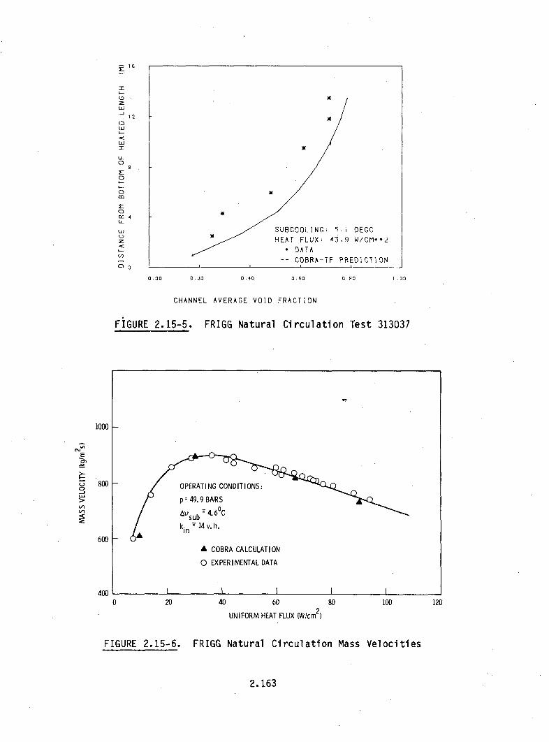
Q6
m
-ij-j 12
U-0)
0
Li-
7-"
V)
)K
)K
SUBCOOLINGý 5.i DEGCHEAT FLUX: A3.9 W/CM.*2
DATACOBRA-TF PREDICTION
0.00 0.20 0.40 0.60
CHANNEL AVERAGE VOID FRACTION
0.RO
FIGURE 2.15-5. FRIGG Natural Circulation Test 313037
1000
E
(- 8000 -JX
600
4000 20 40 60 80 100
UNIFORM HEAT FLUX (W/cm2
FIGURE 2.15-6. FRIGG Natural Circulation Mass Velocities
120
2.163

These results indicate that the methods used for modeling interfacial
shear, two-phase wall shear, two-phase form losses, entrainment and subcooled
boiling are adequate for a boiling channel. These simulations were run on
cycle 10 of COBRA/TRAC.
2.16 SEMISCALE MOD3 TEST S-07-6
Test Series 7 in the Semiscale Mod 3 configuration was performed to
investigate blowdown and reflood transients. Test S-07-6 (Ref. 32) was a 200%
cold leg break with emergency coolant injection in the intact cold leg. The
entire primary system was modeled for the simulation of test S-07-6. The
purpose of the simulation was to demonstrate the capability of the COBRA/TRAC
code to calculate the flow and heat transfer in the system during the blowdown
and reflood transient.
2.16.1 Description of Experiment
The semiscale MOD-3 system consisted of a pressure vessel with simulated
reactor internals, (including 25-rod core and external downcomer assembly) and
two complete primary loops. The intact loop, (which simulated three loops of
a 4-loop plant) consisted of a steam generator, pump and pressurizer. The
broken loop consisted of a steam generator, pump and rupture assembly on the
piping for the inlet cold leg to the downcomer. The primary ECC system was
modeled with high and low pressure injection pumps on the intact loop, and an
ECC accumulator isolated by a pressure activated check valve. The rupture
assembly vented the break to a pressure suppression tank pressurized to
0.25 MPa that simulated the containment.
The initial conditions for the test simulated steady-state reactor
operating conditions. The transient was initiated by subjecting the system to
a double-ended cold leg break. At initiation of blowdown, power to the
primary pumps was reduced and the pump speed was regulated to simulate
coastdown. Power to the electrically heated core was controlled to simulate
the ANS +20% power decay curve. The ECC system was activated at appropriate
times in the transient. The high pressure coolant injection pumps were
started at 3 seconds (at a system pressure of 15.21 MPa) and ran throughout
the test. The low pressure injection° pumps were activated at 31.5 seconds
2.164

after blowdown (at a system pressure of 1.0 MPa). The accumulator check valve
opened at 19 seconds after blowdown, and emptied ECC water into the intact
loop cold leg.
The performance of the system during test S-07-6 was monitored with 235
detectors, with an effective sample rate of 1.917 points per second. Data was
taken for fluid temperature, material temperature, pressure, volumetric flow
rate and density throughout both loops and within the pressure vessel and
external downcomer. The transient lasted -460 seconds.
2.16.2 COBRA/TRAC Model Description
The Semiscale system was modeled in COBRA/TRAC with 29 components.(a)
The model consisted of an intact loop, a broken loop, the ECC system and the
pressure vessel and downcomer. The pressure vessel and downcomer were modeled
with the VESSEL component, and the rest of the system was modeled with the
one-dimensional components.
A diagram of the one-dimensional system components is shown in
Figure 2.16-1. The intact loop model consisted of the hot leg (TEE 1) with
the pressurizer (PRIZER5) attached to the tee branch, a steam generator
(STGEN2, with secondary modeled by FILL 30 and BREAK 31), piping between the
steam generator and pump (PIPE3), a Semiscale pump (PUMP4), and the cold leg,
(TEE9). The ECC components connect to the intact cold leg through the tee
branch. The ECC components were modeled by an accumulator (ACCUMl8), a
pressure-controlled valve (VALVE32), piping from the accumulator to the cold
leg (TEEI6), and piping from the low pressure and high pressure injection
pumps (TEEI7). The injection pumps were modeled as simple mass sources
(FILL33 and FILL34).
(a) The published references for the semiscale system do not provide enoughdata on the physical characteristics of the system to construct anadequate model for COBRA/TRAC. The input data describing the one-dimensional components of the system was obtained from a TRAC-PlA inputdeck. The vessel and downcomer was• mo~deled in COBRA/TRAC using dataobtained from working drawings of the semiscale system.
2.165

2- BREAK 29
0I-4
LUzLU0
4LUI-U,
VALVE 32
TEE 16
FILL33
HIGH PRESSUREINJECTION
zLu
FILL 34LOW PRESSURE
INJECTION
I.-
PUMP8
_Q7BREAK 42TEE 7 f -\
PIPE 41
O FILL 28
PIPE 12
BREAK 26
PIPE10 /\
PRESSUREt VESSEL !:
PIPE 3
TEE 1
FIGURE 2.16-1. COBRA/TRAC Model of Semiscale MOD 3 System
The broken loop model consisted of the hot leg pipe (PIPE12), a steam
generator (STGENll, with-secondary modeled by FILL28 and BREAK29), piping from
the steam generator to the pump (PIPElO), a Semiscale pump (PUMP8), and piping
between the pump outlet and the break assembly (TEE7). The pump side of the
break assembly was modeled with a pipe (PIPE41) and a break (BREAK42); the
downcomer side of the break assembly was modeled with a separate pipe and
break (PIPE6 and BREAK26).
The vessel component modeled the pressure vessel and downcomer with the
multisection channel-splitting logic. A diagram of the VESSEL model is shown
in Figure 2.16-2. The model consists of 36 channels in 10 axial sections.
There are 116 computational cells in the component. The fluid volumes and
flow areas are modeled at values as close as possible to the actual volumes
and flow areas in the Semiscale vessel and downcomer. The heater rods in the
core and the solid structures in contact with the fluid are modeled using the
heat conductor models in the VESSEL module. A one-dimensional mesh is used
except in regions where more channels are required to allow piping connections
or to allow convection paths.
Test S-07-6 began from a steady-state condition intended to simulate a
reactor at full power. The system pressure was at 15.21 MPa, with the core
generating 1.97 MWth, and the system was at equilibrium. The simulation was
run in a steady-state configuration (i.e., without the ECCS components and
with the break assembly modeled as an unbroken straight pipe) for 20 seconds
until the calculation achieved stable equilibrium conditions consistent with
the test initial conditions. Table 2.14 compares measured steady-state test
conditions with the calculated conditions at 20.0 seconds, just before
blowdown was initiated.
2.167

38396 IN.
SECTION 1036
360 IN. 6
S I IOUN
2 3031
1 1 21
22
15
2t11162___ ! 216 IN.
SECTION 619281N.,
SECTION 5 18 N
0SECTION4
I 36 IN.SECTION 3-- - 24 IN.SECTION 2
1? IN.
SECTION 1 Q2FIGURE 2.16-2. COBRA/TRAC Model of Semiscale Pressure Vessel
for Test S-07-6and Downcomer
2.168

TABLE 2.14. Initial Conditions for'Semiscale Test S-07-6
Parameter Test Value COBRA/TRAC Value (at 20 seconds)
Core power (MW) 1.97 1.94
System Pressure (MPa) 15.21 (2163 psia) 16.82 (2393 psia)
Cold leg temperature (K)Intact loop 559 559Broken loop 558 562
Hot leg temperature (K)Intact loop 594.3 593.7Broken loop 593.9 593.5
Loop TemperatureDifference (K)
Intact loop 35.3 34.6Broken loop 35.9 31.4
Core volumetricflow rate (1/sec) 14.26 13.16
The blowdown was initiated by restarting the calculation with the broken
loop cold leg component replaced by the break components modeled as shown in
Figure 2.16-1 and the ECCS components added to the intact loop. Forcing
functions on core power and the pump speed values were used to model the core
power and pump behavior in the transient.
The steam generator secondaries were isolated at the initiation of
blowdown. This was somewhat difficult to model accurately with the TRAC steam
generator module. Even though the main feedwater was shut off, the secondary
side of the steam generators continued to recirculate, providing an unknown,
but not insignificant, secondary flow rate for heat transfer. This was
modeled by providing a reduced but nonzero flow in the FILLs modeling the
steam generator secondaries.
2.16.3 Discussion of Results
Results for the first 70 seconds of the calculation for S-07-6 are shown
in Figures 2.16-3, 2.16-4 and 2.16-5. (In these graphs, the solid line is the
calculation, the asterisks show the data points.) Figure 2.16-3 is a plot of
2.169

2500
2000
U,
1500w
1000w
500
00 10 20 3
TI MI0 40 50 60 70IE (seconds)
Upper Plenum PressureFIGURE 2.16-3.
1000
800
E", 600
I--
400zLU0
200
o 0 10 20 30 40TIME (seconds)
50 60 70
FIGURE 2.16-4. Density at Top of Core
2.170

1000
* DATA
800 -. CODRA!'TRAC Predictien
E K
\ 600
7n400-
wLU
200
00 10 20 30 40 50 60 70
TIME (seconds)
FIGURE 2.16-5. Density in Upper Head
the calculated pressure in the vessel upper plenum versus the measurements
obtained in the experiment. In the blowdown portion of the transient, the
calculation follows the data very well. After 40 seconds, however, errors in
the input caused too much vapor to be generated by heat transfer from the hot
walls in the downcomer, and the pressure was too high. Figure 2.16-4 is a
plot of the density calculated at the top of the core-heated length compared
with the measured values. The calculation is in good agreement with the
data. A similar plot for density in the vessel upper head (Figure 2.16-5) is
also in agreement with the data.
These results indicate that the COBRA/TRAC code is capable of calculating
accurately the behavior of a system undergoing severe blowdown transients.
Good data comparisons require that the system geometry and operating
conditions be modeled correctly.
Developing an accurate and efficient model of the Semiscale system has
proved to be nearly as important as solving the equations in the code
correctly. The large heat transfer surface area-to-volume ratio makes the
2.171
system extremely sensitive to small errors in the modeling input, and the
inadequate documentation of the Semiscale system has made construction of an
accurate model difficult.
The results for the blowdown portion of the transient (i.e., out to
40 seconds) show that the code is calculating the two-phase hydrodynamics
quite well. Later on, however, when the behavior in the downcomer is
dominated by heat transfer from the walls, inaccuracies in the modeling result
in the wrong heat transfer coefficients, and the calculation no longer matches
the data. This simulation was run on cycle 10 of COBRA/TRAC.
2.172

2.17 SEMISCALE MOD2A TEST S-UT-2
Test S-UT-2 performed on Semiscale MOD-2A (Ref. 33) was designed to
simulate the transient behavior of a scaled PWR system under a small break
LOCA (SBLOCA) condition and to study the effects of having emergency core
coolant (ECC) injected into the upper head. Test S-UT-2 was a small (10%)
communicative cold leg break loss-of-coolant experiment performed with upper
head injection. The data from this test was intended for use in assessment of
computer codes developed for full-scale PWR transient calculations.
The purpose of the computer simulation of test S-UT-2 was two-fold. It
verified the capability to model an integrated system with all representative
loop components of a PWR present. In addition, it permitted study of the
capability to predict the system response during a SBLOCA and the effects of
upper head injection (UHI) on core behavior.
2.17.1 Description of Experiment
The MOD-2A system was designed as a small-scale model of the primary
system of a four-loop PWR nuclear generating plant. The system incorporated
the major components of a PWR, including steam generators, vessel, pumps,
pressurizer and loop piping. The intact loop was scaled to simulate three
loops in a PWR, while a broken loop simulated the single loop in which a break
was postulated to occur. Geometric similarity was maintained between a PWR
and MOD-2A, (e.g., in the design of a 25-rod, full-length (3.66-m)
electrically heated core, a full length upper head and upper plenum, the
component layout, and relative elevations of various components). Equipment
in the upper head of the MOD-2A vessel was designed to simulate the fluid flow
paths found in a PWR with the capability of injecting ECC into the upper head.
A diagram of the Semiscale Mod-2A system, as configured for Test S-UT-2,
is shown in Figure 2.17-1 with major components identified. The break was
located in the broken loop cold leg between the pump and the vessel and was
communicative in nature. The break orifice is shown in detail in
Figure 2.17-2. The break size was 0.228 cm2 , which is volumetrically scaled
to represent 10% of the area of a cold leg pipe in a PWR. In order to be
2.173

Type II steam generator(intact loop)
Type II steam generator(broken loop)
Pressuresuppressiontank Hot leg
Pressurizer
leg
Pump suction
Break assembly
PressuresuppressionheaderPump suction
Vessel downcomer
FIGURE 2.17-1. Semiscale MOD-2A System for Small Break LOCA
2.174

F10,144
I2.5-0
All dimensions in cm
FIGURE 2.17-2. Detail of Small Break Orifice in Test S-UT-2
representative of an orifice-like break in a PWR pipe, the orifice was
designed as sharp-edged with a length-to-diameter ratio of 0.27.
Internally heated electric rods are used to simulate the nuclear rods of
a PWR. The rods are geometrically similar to nuclear rods with a heated
length of 3.66 m and an outside diameter of 1.072 cm. The axial power profile
for the rods has a step cosine shape with a 1.55 peak-to-average power
factor. Twenty-three heated rods were powered uniformly. Two diagonal rods
were unpowered. The total core power was 1.91 MW which yielded a maximum
linear heat generation rate of 35.19 kW/m. Penetrations into the upper head
consist of a perforated ECC injection tube, a bypass line from the top of the
downcomer, a simulated control rod guide tube, and two simulated support
columns.
The test was initiated from steady state conditions by rupturing discs
downstream of the break orifice to breach the system pressure boundary.
Transient core power control and the intact and broken loop pump speed
controllers were initiated by a pressure trip 1 sec after the pressurizer
2.175

pressure reached 12.41 MPa. The pressure suppression system (PSS) tank
pressure was held initially at 1030 kPa, then ramped down to 280 kPa from 50
to 90 sec and held there for the remainder of the test. (This was done to
keep the downstream drag screen measurement within range while keeping the
flow choked at the break orifice.) Both intact and broken loop steam
generator feedwater and steam valves were sequenced to close 1 sec after the
pressurizer pressure reached 12.41 MPa.
The system pressure decreased continuously throughout the test. The
high-pressure injection system (HPIS) pump began injecting ambient temperature
water into the intact loop cold leg 2 sec after rupture. The system voided
from the upper elevations downward, and by 200 sec the loops had cleared of
liquid while liquid remained in the vessel and downcomer below the cold leg
elevation. Between 30 and 90 sec, water in the pump suction of each loop
formed a seal, preventing steam flow around the loops. This caused a
depression of the vessel liquid level and a brief period of dryout and minor
temperature excursions throughout most of the core. These hot spots were
re-wet after the loop seals voided.
When the pressure dropped to 2.98 MPa at 345 sec, the intact loop
accumulator began injecting water into the cold leg. Heater rod cladding
temperatures followed system saturation temperature until the end of the
test. The low pressure injection system (LPIS) began injecting water at
2395 sec at a system pressure of 1.15 MPa.
2.17.2 COBRA/TRAC Model Description
Figure 2.17-3 shows the COBRA/TRAC model of the semiscale MOD-2A system
used for Test S-UT-2. The intact and broken loops and the upper head
injection systems were represented by one-dimensional components. The
pressure vessel and downcomer was represented by a VESSEL component. The high
pressure and low pressure injection systems were modeled as mass sources by
two FILL components. The UHI system and intact loop accumulator were modeled
by the ACCUM components. The steam generator model includes the primary side
U-tube and the secondary side tube region. The steam separator, steam dome
and downcomer were not explicitly modeled due to the limitation of the one-
dimensional component steam generator model. To provide a reasonable
2.176

ACCUM 38BREAK 29
JUN 22
BREAK 31
VALVE 35JUN 36
JUN 39
PI PE 37
FILL 28
JUN21,
PRIZER 5
JUN 20 23 JUN ? + + JUN 3PI PE 12 JUN 9
-~1
JUN 19 JUN 13 JUN 5
JUNPIPE 10 JUN 31 JUN
PIPE 3
BREAK 26FILL 34(H?IS)
DOWNCONiLRTEE 17 JUN'
35VALVE 32
ACCUM 18
FIGURE 2.17-3. COBRA/TRAC Model of Semiscale MOD2A System

secondary side boundary condition, the feedwater flow rates and temperatures
were adjusted to account for the recirculation flow. Steam discharge pressure
histories were set to the measured values to minimize the errors associated
with the heat transfer characteristics between the primary and secondary
loops, since the downcomer and steam separator were not explicitly modeled.
Figure 2.17-4 shows the detailed noding diagram of the vessel
component. The vessel is divided into 10 vertical sections. Section 1 models
the lower plenum which contains two channels (1 and 2) separated by a gap
(GI). Channel 1 is an annular volume that connects to the downcomer and
channel 2 is directly below the core.
Sections 2 and 3 model the core inlet and lower part of the downcomer.
Section 2 contains channels 3 and 4 and rods 3 and 4. The rods are modeled to
account for heat transfer through the metal walls and insulation liners.
Section 4 contains the vessel core, the heated rods inside the core and the
downcomer. Section 5 models the upper core plate. Sections 6, 7 and 8 model
the upper plenum, downcomer inlet and downcomer bypass line. The two support
columns are modeled by a single channel (channeis 15, 21 and 30 stacked one on
top the other through sections 6, 7 and 8). Channel 15 communicates with the
core at the lower end of the support column, and channel 30 with the upper
head at the upper end. The guide tube is modeled by stacking channels 14, 20,
29 and 33. It also communicates with the core at the lower end. Its open
upper end is inside the upper head.
Sections 9 and 10 model the upper head. Channels 35 and 38 represent the
upper head injection (UHI) tube. The tube is perforated to allow water from
the UHI accumulator to be injected into the upper head. These openings are
modeled by gaps 4 and 5.
Except through guide tube and support columns, there is no connection for
fluid flow between channels 27 and 34. The noding for the break nozzle is
shown in Figure 2.17-5.
2.17.3 Discussion of Results
With the given core power level, pressurizer saturation temperature, pump
speed and steam generator secondary boundary conditions as input, the
calculation was started. Steady-state conditions were assumed to be
2.178
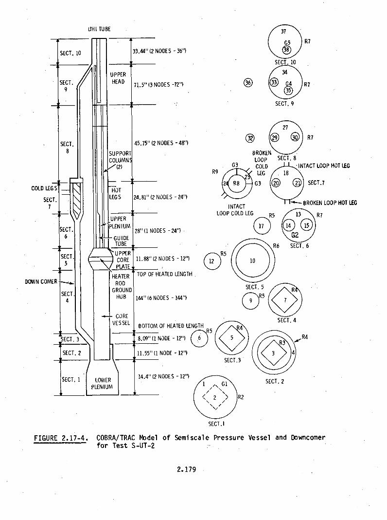
UHI TUBE
SECT. 10
SECT..9
aR7
33.44" (2 NODES - 36")
UPPERHEAD
SECT.8
COLD LEGS
SECT.7
DOWN COMER
SE CT.
SUPPORTCOLUMNS
(2)
HOTLEG S
JjUPPERPLENIUM
GUIDETUBE
U PPER- CORE
PLATE
71.5" (3 NODES -72")
45.75" (2 NODES -48")
24.81" (2 NODES - 24!')
28" (1 NODES - 24")
11.88" (2 NODES - 12") C12
TOP OF HEATED LENGTH
144" (6 NODES - 144")
BOTTOM OF HEATED LENGTH
8.09" (1 NODE 12") ,jR
11.55" (1 NODE - 12")
14.4" (2 NODES - 12")
27
® ®R7
BROKENLOOP SECT. 8COLD -INTACT LOOP HOT LEG
R.LEG 18
2 G3 G3 SECT.7
I"NTACT BROKEN LOOP HOT LEGLOOP COLD LEG R5 13 R7
1 G 2
,-~- R R6 SECT. 6
R7
SECT. 9
SECT.4
HEATERROD
GROUNDHUB
4COREVESSEL
SECT. 3
SECT. 2
SECT. 1 LOWERPLEN I UM
SECT.3
Q/I G I"< E2> R2
SECT. I
SECT. 2
FIGURE 2.17-4. COBRA/TRAC Model offor Test S-UT-2
Semiscale Pressure Vessel and Downcomer
2.179
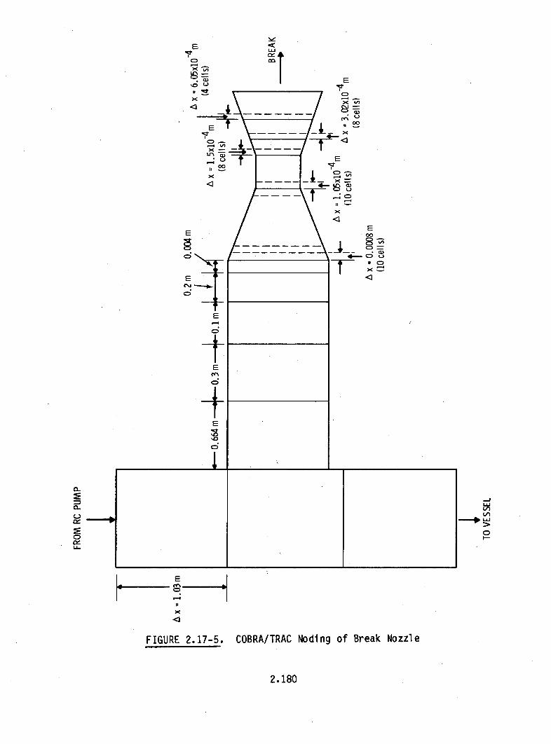
E <xE
x L;
1'
C X
E
E
o..-
5X=
00
0CD
(-C)
E
FIGURE 2.17-5. COBRA/TRAC Noding of Break Nozzle
2.180
established when all major parameters reached steady values. The steady-state
parameters established before the blowdown was started are listed in
Table 2.15.
The calculated steady-state values do not exactly match the measured
values. It is believed that the discrepancies were caused by the modeling of
the steam generators. The steam generators were modeled without the steam
separator and downcomer, therefore errors in the computed recirculation rate
caused errors in the prediction of the temperature drop across the U-tubes.
This caused errors in the core enthalpy and flow rate. The system pressure
mismatch was apparently caused by the pressurizer modeling.
After steady-state conditions were established, *the blowdown was
started. The calculated results are given in Figures 2.17-6 through 2.17-12.
Figure 2.17-6 gives the system pressure as a function of time. The
calculated pressure follows the initial rapid depressurization with reasonable
accuracy. After the initial depressurization, the curve starts to diverge
gradually from the measured values, and the calculation gives a higher
pressure as the transient progresses. This deviation is due to an incorrect
prediction of the break mass flow rate predicted by TRAC.
Figure 2.17-7 gives the collapsed liquid level in the vessel downcomer as
a function of time. The shift relative to the measured data is probabily due
to too much heat transfer from the steam generator secondary to the primary
side; i.e., higher system pressure, which suppresses the core liquid level
through hot leg connections and keeps the downcomer liquid high for a longer
period. However, the decrease of downcomer liquid level from pump seal
clearing and subsequent liquid level equalization with the core were predicted
in the calculated results.
The pump suction clearing occurred at about 120 sec for the broken loop
and 230 sec for the intact loop; compared to about 90 sec for both loops from
measurements. This also contributed to the delayed behavior of the downcomer
liquid level history.
2.181

TABLE 2.15. Initial Conditions for Semiscale Test S-UT-2
COB RA/TRACValue (at 20s)
TestValue
System pressure (psia)
Core inlet flow (Ibm/s)
Core AH (Btu/lbm)
Intact loop steamgenerator primaryside AT (K)
Broken loop steamgenerator primaryside AT (K)
2310
21.4
82.6
28.8
2250
23.2
78.2
34.1
31.635.0
15.0
0.
CD,wh0.
10.0
5.0
0.0 L0 100 200
TIME (s)300
FIGURE 2.17-6. System Pressure
2.182

U
-J
ww-Ja50
600
500
400
300
200
100
0
COLD LEGCENTER LINE
(
0 100 200 300TIME (s)
FIGURE 2.17-7. Collapsed Liquid Level in Semiscale Downcomer Pipe
400
LU
cc
0
z
-Jw
w.-J(a5,0,
350
300
250
200
150
100
0 100 200TIME (s)
300
FIGURE 2.17-8. Collapsed Liquid Level in Semiscale Core
2.183

Uj
-j
-LI
w
(w(.D.
300
250
200 -
150
100
50
000
FIGURE 2.17-9.
100 200 300TIME (s)
Collapsed Liquid Level in Upper Head
w
I-
w
560
540
520
500
480
4600 100 200
TIME (s)
FIGURE 2.17-10. Upper Head Fluid Temperature
300
2.184

ý, 640w 6 2 0
600Ir 580
560 _._..-540
I= 520 -
<€500u THERMCOUPLE THV* C2 + 321
Z 480 - COBRA/TRAC AVERAGE RODwc 460L)440 0 10 20 30
TIME (s)
FIGURE 2.17-11. Rod Temperature at the Core Mid-Plane
680
660 THERMOCOUPLE THV*
S640 C4 + 187
620; THERMOCOUPLE THV*
1B1 + 183x < /COBRA/TRAC5j•-600
-540-
520-
0 100 200 300TIME (s)
FIGURE 2.17-12. Rod Temperature Near Top of Core
2.185
Figure 2.17-8 gives the core liquid level as a function of time.
COBRA/TRAC calculated more liquid in the core than the test showed because of
the higher heat transfer from the steam generators and the delayed pump
suction clearing. In addition, the core level recovery due to clearing of
pump suction occurred late in the transient. The higher liquid level from the
beginning of blowdown up to 100 sec is mainly due to the slower blowdown
caused by high energy input from the steam generators and a poor break flow
prediction. Figure 2.17-9 gives the upper head liquid level. In this region,
the calculation follows the measurements reasonably well. The higher system
pressure resulted in a slower and longer drain of the upper head accumulator
(the accumulator injection was terminated at about 185 sec instead of the
measured 140 sec), causing the delayed drop shown in the curve.
Figure 2.17-10 gives the upper head fluid temperature as a function of time.
The temperatures were plotted for the fluid at 122 cm above the bottom of the
upper head. Condensation due to the cold UHI water and subsequent heatup due
to the steam upflow from the guide tube are illustrated by the repeated
fluctuations in the fluid temperature. The fluid temperature after UHI was
terminated essentially followed the saturation temperature curve. Because of
the higher system pressure, the fluid temperature is also higher during this
period.
Figures 2.17-11 and 1.17-12 give the heater rod clad temperatures at two
different elevations, one at about the mid-plane, another close to the
outlet. Comparisons were made between an average rod as calculated by
COBRA/TRAC and thermocouple measurements of selected rods. Again the trend is
consistent with the calculated higher system pressure. In the thermocouple
measurements some rods experienced dryout and others did not. The code
calculation for the average rod did not show dryout. There are two possible
causes for this inconsistency. The CHF correlations in the code may not be
adequate for the calculations of the dryout heat transfer. This, however, is
unlikely because the code has been tested on other sample cases and showed
good comparison on rod temperature calculations under similar conditions.
Another possibility is that because of the calculated slower blowdown there
was a sufficient inventory of liquid inside the core to prevent the dryout
from occurring.
2.186

Different cell arrangements in the break nozzle were tested. Some with
more cells than the one presented in Figure 2.17-5, some with less. All of
them gave about the same amount of break flow during the initial stage of
blowdown. Therefore, the prediction of break flow is a result of modeling
deficiencies in the TRAC implicit pipe component and not in the nodalization
at the break.
It was found that lowering the secondary feedwater temperature in the
steam generator (below Tsat) increased the core maximum uncovery. In the
current one-dimensional steam generator model, the feedwater temperature input
is fixed rather than a function of time, and the recirculation flow is input
rather than consistently calculated. The inaccuracies this introduced in the
calculation may have caused the calculated core liquid level to differ from
the measured value. °
In general, given the constraints of modeling the steam generators and
the break flow the results from the COBRA/TRAC calculation produced the
correct trends of the data. Important phenomena such as pump suction
clearing, upper head condensation and heatup, the downcomer liquid level
equalization, and the core liquid level recovery, were demonstrated by the
calculation. The shifted (with respect to time) behavior of different
components all could be explained by the heat transfer deviations from
secondary to primary loops due to the steam generator model and by the error
in the calculated break mass flow rate.
To correct the deficiency caused by the simplified steam generator model,
the same simulation has been repeated with the one-dimensional steam generator
model replaced by a three-dimensional model using the VESSEL module. The
VESSEL module is capable of explicitly simulating the steam generator
downcomer, the steam dome and the steam separator. With this improvement, the
heatbalance between the primary and secondary loops during transient should
be calculated more accurately. A new break model has also been implemented
that should provide an improved prediction of break mass flow. Results of
this more recent calculation will be reported in a different document. This
simulation was run on cycle 8.
2.187

2.18 WESTINGHOUSE UPPER HEAD DRAIN TEST
The Westinghouse Drain Test facility was designed to simulate the upper
head of a pressurized water reactor (PWR) vessel with upper head injection
(UHI). A COBRA/TRAC simulation of the drain test assessed the code's ability
to predict upper head draining in a UHI system. Performance was evaluated by
comparing the calculated draining rate, temperature and pressure with
experimentally measured proprietary data. The results of this simulation were
used to develop the model for the upper head for simulation of a PWR vessel
with UHI.
2.18.1 Description of Experiment
The UHI reactor vessel was designed to deliver water to the upper head of
the'vessel during a loss-of-coolant accident. The objective of the
Westinghouse Drain Test was to demonstrate that the upper head will drain of
water. Designers predict that the hydrostatic head forces water from the
upper head into the core. At the same time, steam flows from the core and
upper plenum through the control rod guide tubes to the upper head of the
vessel.
The Westinghouse Drain Test facility consisted of a full-scale PWR guide
tube with the upper plenum, upper head volume and support columns to simulate
the vessel on a per guide tube basis. Two pipes were used as the support
columns. The pipes were orificed to simulate one full-scale and one-half
scale support column since a PWR vessel contains one and one-half support
columns per guide tube. A steam chamber simulated the upper plenum of the
core during the reflood stage of a loss-of-coolant accident. Saturation
conditions were maintained by a continuous flow of steam through the
chamber. A check valve in the exhaust line prevented air from entering the
test section during testing.
The upper head and support columns were initially filled with subcooled
water. A plug valve at the top of the guide tube and flapper valves at the
bottom of the support columns were opened simultaneously to begin the test.
Water from the upper head drained through the support column to the upper
plenum as steam from the upper plenum rose through the guide tube to the top
2.188
of the upper head. The test was terminated when the water level in the upper
head reached the top of the support columns.
2.18.2 COBRA/TRAC Model Description
Although only the vessel component was needed in this simulation a PIPEcomponent is required in every COBRA/TRAC model. The pipe in this model
connected a FILL component to the top of the vessel component. A zero
velocity boundary condition on the FILL component prevented flow through the
pipe. The net effect of the PIPE component was to add 0.03% to the volume of
the upper head.
Thermal non-equilibrium was an important feature in this simulation
because saturated steam comes into contact with subcooled water at the top of
the guide tube. Heat transfer to the wall of the vessel was ignored. The
carbon steel test section was heated with steam flow before each test, and the
test was completed in a relatively short period of time. Heat transfer
between the wall and the fluid was negligible.
The COBRA/TRAC model of the Westinghouse Drain Facility consisted of
28 cells in five channels. A schematic diagram of the model is shown in
Figure 2.18-1. Channels 1 and 3 model the guide tube. Area changes due to
intermediate guide plates were modeled by loss coefficients. The loss
coefficients used were calculated from the area change, thickness of orifice
and hydraulic diameter of the channel. The full and half-scale support
columns were combined into channel 2. The flow area of the channel was the
sum of the flow areas for the two support column tubes.
Since two support columns were being modeled by one channel, the loss
coefficients for the support columns were combined. Each support column had
an experimentally measured loss coefficient. The loss coefficient for input
was calculated to produce the same pressure drop for the same total mass flow
through the two support columns. Channels 4 and 5 modeled the upper head. A
pressure and enthalpy boundary condition below channels 1 and 2 modeled the
steam chamber of the test facililty.
2.189

+ 52 CELLS
_t • UPPER HEAD
6 CELLS 3
GUIDE TUBE
8 CELLS 2
1 •SUPPORT COLUMN
P(t), H(t) j UPPER PLENUM
FIGURE 2.18-1. COBRA/TRAC Model of Westinghouse Upper Head Test Section
2.18.3 Discussion of Results
COBRA/TRAC calculations of drain rate, temperature at the top of the
support columns, and pressure at the top of the guide tube are compared with
measured data from the Westinghouse Drain Test in Figures 2.18-2, 2.18-3 and
2.18-4. (The numbers have been removed from the axes because the information
is proprietary.)
Drain rate is reported as upper head fluid level versus time in
Figure 2.18-2. The maximum difference between calculated and measured fluid
level is 3% of the initial level at the beginning of the transient.
Approximately half of the difference is accounted for by a small amount of
liquid that fell into the guide tube at the beginning of the transient.
Liquid fell into the guide tube because the orifice at the top of the guide
tube was modeled by a loss coefficient without an area reduction. The loss,
coefficient provided the right pressure drop, but the velocity was wrong. The
calculated vapor velocity out the top of the guide tube was much lower than
that in the experiment. The lower velocity allowed a small amount of
2.190
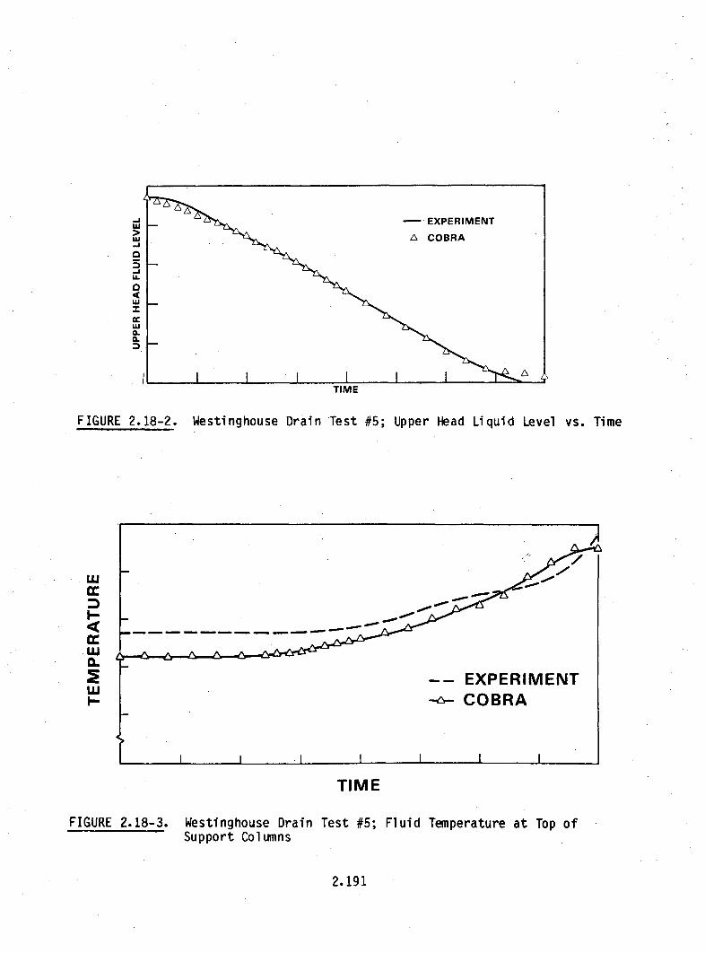
-iLU
IxU-
CL
FIGURE 2.18-2.
wj
I-j
Wj
TIME
Westinghouse Drain Test #5; Upper Head Liquid Level vs. Time
TIME
FIGURE 2.18-3. Westinghouse Drain Test #5; Fluid Temperature at Top ofSupport Columns
2.191

...... . ... ... A..
uwc A -EXPERIMENT
COBRA
TIME
FIGURE 2.18-4. Westinghouse Drain Test #5; Pressure at Top of Guide Tube
liquid to fall into the guide tube. An area variation can be used to model
the orifice, but the increase in vapor velocity would severely limit the time
step size.
Figure 2.18-3 shows the fluid temperature at the top of the support
columns as a function of time. The maximum difference between measured and
calculated temperature is 5°F at test initiation. The reason for the
difference is a 10°F temperature gradient from the top to the bottom of the
upper head. COBRA/TRAC was initialized with the average upper head liquid
temperature. The temperature at the top of the support columns was actually
5°F higher than the average temperature. The calculated temperature
approached the measured temperature as the transient proceeded.
Pressure at the top of the guide tube is shown in Figure 2.18-4. The
calculation of pressure over the first third of the transient does not agree
with the measured pressure. The maximum difference between measured and
calculated values is 21%. The difference is caused by the location of the
pressure measuring device in the upper head. The pressure tap was located at
the top of the upper head directly above the support columns. COBRA/TRAC
2.192

computes the pressure above the guide tube as an average over the entire area
of the upper head. Since saturated steam was condensing in the subcooled
liquid of the upper head it is likely that a local pressure in the upper head
is considerably different than an averaged value.
The liquid level was below the top of the guide tube in the final two-
thirds of the transient. Condensation no longer played a significant role in
determining the pressure above the guide tube. Figure 2.18-4 shows that when
the liquid level fell below the top of the guide tube the measured and calcu-
lated pressures above the guide tube agreed well. The maximum difference
between measured and calculated pressure above the guide tube in the final
two-thirds of the transient was less than 2%.
The calculation of drain rate, pressure and temperature in the upper head
agrees well with measured data from the Westinghouse Drain Test. These
results indicate that the model used in this simulation can predict the
behavior of upper head draining in the simulation of a complete PWR with UHI.
2.193

REFERENCES
1. Liles, D. R., et al., Los Alamos Scientific Laboratory, "TRAC-PD2, AnAdvanced Best Estimate Computer Program for PWR LOCA Analysis," USNRReport NUREG/CR-2054, April 1981.
2. Lovell, T. W.,"The Effect of Scale on Two-Phase Countercurrent FlowFlooding in Vertical Tubes," M.S. Thesis, Thayer School of Engineering,Dartmouth College, Hanover, New Hampshire, June 1977.
3. Hsieh C., S. G. Bankoff, R. S. Tankin and M. C. Yuen, "CountercurrentAir/Water and Steam/Water Flow above a Perforated Plate," Final Report,NUREG/CR-1808, Northwestern University, November 1980.
4. Crowley, C. J. and J. A. Block and C. N. Cary, Downcomer Effects in a1/15-Scale PWR Geometry, Experimental Data Report, CREARE, Inc.,NUREG-0281, 1977.
5. Carbiener, W. A., et al., Steam-Water Mixing and System HydrodynamicsProgram Quarterly Progress Report, July 1 - September 30, 1971, BMI-NUREG-1987, Battelle-Columbus Laboratories, Columbus, Ohio, 1977.
6. Carbiener, W. A., et al., Steam-Water Mixing and System HydrodynamicsProgram, Quarterly Progress Report, January 1 - March 31, 1977, BMI-NUREG-1972, Battelle Columbus Laboratories, Columbus, Ohio, 1977.
7. Collier, R. P., et al., Steam-Water Mixing and System HydrodynamicsProgram, Quarterly Progress Report, July 1 - September 30, 1977,NUREG/CR-0526, BMI-2011, Battelle-Columbus Laboratories, Columbus, Ohio,1978.
8. Rust, K. and P. Ihle, Warmeubergang und Kuhlmittelstromung beim Flutenblockierter Anordnungen, Kernforschungszentrum Karlsruhe, Republic ofWest Germany, 1980.
9. Ihle, P., Flooding Experiments in Blocked Arrays, FEBA, Recent Resultsand Future Plans, presented at the Eighth Water Reactor Safety Research.Information Meeting, October 27-31, 1980, Gaithersburg, Maryland, 1980.
10. Rosal, E. R., L. E. Hochreiter, and M. F. McGuire,ý "FLECHT Low FloodingRate Cosine Test Series Data Report," WCAP-8651, Westinghouse ElectricCorporation, 1975.
11. Rosal, E. R., C. E. Conway, and M. C. Kocpinevich, "FLECHT Low FloodingRate Skewed Test Series Data Report," WCAP-9108, Westinghouse ElectricCorporation, 1977.
12. Phillips, L. E., letter to U. S. Standard Problem Participantstransmitting "Standard Problem No. 9 (FLECHT-SEASET) SpecificationReport." Nuclear Regulatory Commission, 1979.
R.1
13. Hochreiter, L. E., et al., Power FLECHT-SEASET Unblocked Bundle, Forcedand Gravity Reflood Task: Task Plan. Report. NRC/EPRl/WestinghouseReport No. 3, 1978.
14. Mohr, C. L., et al., "Prototypic Thermal-Hydraulic Experiment in NRU toSimulate Loss-of-Coolant Accidents," PNL-3681 NUREG/CR-1882, PacificNorthwest Laboratory, Richland, Washington, 1980.
15. Mohr, C. L., et al., "Loss-of-Coolant Accident Simulations in theNational Research Universal Reactor, Safety Analysis Report," PNL-3093NUREG/CR-1208, Pacific Northwest Laboratory, Richland, Washington, 1981.
16. Banner, J. 0., et al., Materials Test-2 LOCA Simulation in the NRUReactor. NUREG/CR-2509, PNL-4155. Pacific Northwest Laboratory,Richiand, Washington. Prepared for.. U.S. Nuclear Regulatory Commission,1982.
17. Russcher, G. E., et al., LOCA Simulation in the NRU Reactor: MaterialsTest-i. NUREG/CR-2152, PNL-3835. Pacific Northwest Laboratory,Richiand, Washington, Prepared for the U.S. Nuclear RegulatoryCommission, 1981.
18. Brand, B., R. Kirmse, and W. Winkler, Refill and Reflood Experiment in aSimulated PWR Primary System (PKL). Specification, 1979. OECD-CSNI LOCAStandard Problem No. 10. Kraftwerk Union Report R513.
19. Brand, B., R. Mandl, and H. Schmidt, PKL Refill and Reflood ExperimentSelected Results from Test K9, 1979, Kraftwerk Union Report R51/22/79.
20. Kirmse, R. E., Status of PKL Activities. Presented at 6th Meeting of theCSNI Working Group on Emergency Core Cooling in Water Reactors, 1979.
21. Hirano, K., et al., "Quick-Look Report on Large Scale Reflood Test-2 -CCTF C1-2 (Run 011)," JAERI-memo 8530, Japan Atomic Energy ResearchInstitute, October 1979.
22. Cook, D. H., Local Condensation Rates for the Countercurrent StratifiedFlow of Steam and Water in a Vertical Chann6l, M. S. Thesis, NorthwesternUniversity, Evanston, Illinois, 1979.
23. Lahey, R. T. Jr., Two-Phase Phenomena in Nuclear Reactor Technology.Quarterly Progress Report No. 8, NUREG/CR-0418, Rensselaer PolytechnicInstitute, Troy, New York, 1978.
24. Serizawa, A., et al., "Turbulent Structure of Air-Water Bubbly Flow-II.Local Properties." Int. J. Multiphase Flow. 2(3):235-246, 1976.
25. Lahey, R. T. Jr., et al., Subchannel and Pressure Drop Measurements in aNine-Rod Bundle for Diabatic and Adiabatic Conditions. Technical ReportNo. GEAP-13049, General Electric Company, San Jose, California, 1970.
R.2

26. Sim, S. K., Analysis of Phase Distribution Mechanisms in Turbulent Two-Phase Pipe Flow. M. S. Thesis, Rensselaer Polytechnic Institute, Troy,New York, 1977.
27. Bennett, A. W., et al., Heat Transfer to Steam-Water Mixtures Flowing inUniformly Heated Tubes in Which the Critical Heat Flux has BeenExceeded. UKAEA Report No. AERE-R5373, 1967.
28. Nylund, 0., et al., Hydrodynamic and Heat Transfer Measure on a FullScale Simulated 36-Rod Marviken Fuel Element with Uniform Heat FluxDistribution. ASEA and AB Atomenergl Report FRIGG-2, R4-447/RTL-1007,1968.
29. Henstock, W. H., and T. J. Hanratty, "The Interfacial Drag and the Heightof the Wall Layer in Annular Flows." AIChE Journal, Vol. 22, No. 6,pp. 990-1000, 1976.
30. Wallis, G. B., "Annular Two-Phase Flow, Part I: Simple Theory," Journalof Basic Engineering, (March 1970).
31. Dukler, A. E., Flow Regime Transitions for Vertical Upward Gas LiquidFlow: A Preliminary Approach Through Physical Modeling. NUREG-0214,Progress Report, 1977.
32. Esparza, V., et al., Experiment Data Report for Semiscale MOD-3 IntegralBlowdown and Reflood Heat Transter Test S-O7-6 (Baseline Test Series),NUREG/CR-0467, IREE-122b, EG&G Idaho, Inc., Idaho National EngineeringLaboratory, prepared for U.S. Nuclear Regulatory Commission and U.S.Department of Energy, January 1979.
33. Blakely, J. E. et al., "Quick Look Report for Semiscale MOD-2A TestS-UT-2", EG&G-SEMI-5333, Idaho National Engineering Laboratory, 1981.
R.3


APPENDIX A
DESCRIPTION OF CODE VERSIONS

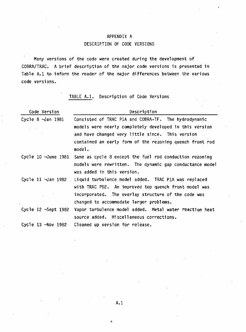
APPENDIX A
DESCRIPTION OF CODE VERSIONS
Many versions of the code were created during the development of
COBRA/TRAC. A brief description of the major code versions is presented in
Table A.1 to inform the reader of the major differences between the various
code versions.
TABLE A.1. Description of Code Versions
Code Version
Cycle 8 -Jan 1981
Cycle 10 -June 1981
Cycle 11 -Jan 1982
Cycle 12 -Sept 1982
Cycle 13 -Nov 1982
Description
Consisted of TRAC PlA and COBRA-TF. The hydrodynamic
models were nearly completely developed in this version
and have changed very little since. This version
contained an early form of the rezoning quench front rod
model.
Same as cycle 8 except the fuel rod conduction rezoning
models were rewritten. The dynamic gap conductance model
was added in this version.
Liquid turbulence model added. TRAC PlA was replaced
with TRAC PD2. An improved top quench front model was
incorporated. The overlay structure of the code was
changed to accommodate larger problems.
Vapor turbulence model added. Metal water reaction heat
source added. Miscellaneous corrections.
Cleaned up version for release.
A.1

NUREG/CR-3046 Vol. 4PNL-4385R4
DISTRIBUTION
No. ofCopies
OFFSITE
No. ofCopies
ONSITE
335 U.S. Nuclear RegulatoryCommi ssi on
Division of TechnicalInformation and DocumentControl
7920 Norfolk AvenueBethesda, MD 20014
5 James HanU.S. Nuclear Regulatory
Commission7915 Eastern Ave.M/S 1130-SSSilver Spring, MD 20910
50 Pacific Northwest Laboratory
Mj Thurgood (43)Publishing Coordination (2)Technical Information ED (5)
Di st-I


NRC FORM 335 1. REPORT NUMBER (Ausied by OOC)U.S. NUCLEAR REGULATORY COMMISSION111-811 BIBLIOGRAPHIC DATA SHEET NUREG/CR-3046, Vol. 4
4, TITLE A N D SUBTITLE (Add Volume No., if appropriare) 2. (Leave blank)COBRA/ TRAC - A Thermal Hydraulics Code for T-ransientAnalysis of Nuclear Reactor Vessels and Primary Coolant 3. RECIPIENT'S ACCESSION NO.Systems - Vol. 4: Developmental Assessment and Data
7. AUTHOR(S) S .H. Bian .5. DATE REPORT COMPLETEDM.J. Thurgood, T.E. Guidotti, G.A. Sly, J.M. Kelly, MONTH IYEARR.J. Kohrt, K.R. Crowell, C.A. Wilkins, J.M. Cuta, November 1982
9. PERFORMING ORGANIZATION NAME AND MAILING ADDRESS (include Zip Code) DATE REPORT ISSUED
Pacific Northwest Laboratory MONTH IY9ARPO Box 999 March .1983Richland, Washington 99352 6. tLeave Wank)
8. (Leave blank)
12. SPONSORING ORGANIZATION NAME AND MAILING ADDRESS (Include Zip Code) 10. PROJECT/TASK/WORK UNIT NO.
Division of Accident EvaluationOffice of Nuclear Regulatory Research 11. FIN NO.U.S. Nuclear Regulatory Commission FIN B2391Washington, DC 20555
1. TYPE OF REPORT PERIOD COVERED (Inclusive dAes)Computer Code Manual I
15. SUPPLEMENTARY NOTES 14. (Leave olanki
16. ABSTRACT (200 words or less)The COBRA/TRAC computer program has been developed to predict the thermal-hydraulicresponse of nuclear reactor primary coolant systems to small and large break loss-of-coolant accidents and other anticipated transients. The code solves the compressiblethree-dimensional, two-fluid, three-field equations for two-phase flow in the reactorvessel. The three fields are the vapor field, the continuous liquid field, and theliquid drop field. A five-equation drift flux model is used to modelfluid flow in theprimary system piping, pressurizer, pumps, and accumulators. The heat generation rateof the core is specified by input and no reactor kinetics calculations are includedin the solution. This volume documents the major data comparisons made with COBRA/TRAduring the process of code development. These data comparisons wereextremely usefuldetecting programming errors and defining deficiencies in the code's physical models.The data comparisons presented in this volume document the resultsobtained ondevelopmental versions of the code. A separate document will be released at a laterdate containing data comparisons run on the final released version of the code.
17. KEY WORDS AND DOCUMENT ANALYSIS 17a. DESCRIPTORS
17b. IDENTIFIERS;OPEN-ENDED TERMS
18. AVAILABILITY STATEMENT 19ýJSEJURITY JLASa (This rPOPrt) 21. NO. OF PAGES
Unlimited (This o.geJ 22. PRICE
S
NRC FORM 335 11-.81)
* U.S. GOVERNMENT PRINTING OFFICE: 1983-381-297:3011


UNITED STATESNUCLEAR REGULATORY COMMISSION
WASHINGTON, D.C. 20555
FOURTH-CLASS MAILPOSTAGE & FEES PAID
USNRCWASH. 0 C
PERMIT No G76
OFFJCIAL BUSINESSPENALTY FOR PRIVATE USE. $300