Numerically safe lower bounds for the Capacitated Vehicle

Routing Problem ∗

Ricardo Fukasawa1 and Laurent Poirrier1

1Department of Combinatorics & Optimization, , University of Waterloo, Waterloo, ON,Canada N2L 3G1 , {rfukasawa,lpoirrier}@uwaterloo.ca

May 13, 2016

Abstract

The resolution of integer programming problems is typically performed via branch-and-bound. Nodes of the branch-and-bound tree are pruned whenever the corresponding subprob-lem is proven not to contain a solution better than the best solution found so far. This is a keyingredient for achieving reasonable solution times. However, since subproblems are solved infloating-point arithmetic, numerical errors can occur, and may lead to inappropriate pruning.As a consequence, optimal solutions may be cut off. We propose several methods for avoidingthis issue, in the special case of a branch-cut-and-price formulation for the Capacitated Vehi-cle Routing Problem (CVRP). The methods are based on constructing dual feasible solutionsfor the LP relaxations of the subproblems and obtaining, by weak duality, bounds on theirobjective function value. Such approaches have been proposed before for formulations with asmall number of variables (dual constraints), but the problem becomes more complex whenthe number of variables is exponentially large, which is the case in consideration. We showthat, in practice, besides being safe, our bounds are stronger than those usually employed,obtained with unsafe floating-point arithmetic plus some heuristic tolerance, all of this at anegligible computational cost. We also discuss some potential advantages and other uses ofour safe bounds derivation.

1 Introduction

Mixed-integer programming (MIP) is a fundamental tool in operations research. Great progresshas been made in MIP solvers like CPLEX (see [20]), to the point that MIPs are nowadaysoften used as subroutines for other problems (as an example see [13]). It is now common foreven problems with hundreds of thousands of variables and constraints to be considered easy(see [23]).

However, most MIP solvers work with floating-point (FP) arithmetic, which implies thatsome of the decisions that are taken by the algorithms implemented within them can beincorrect. This is due to the intrinsic numerical errors that accompany FP arithmetic ([17]).

Some recent works ([30, 12]) have shown that indeed these numerical errors can lead tocommercial solvers returning incorrect solutions. They highlight some of the potential con-sequences that these can have. To give an idea of one such issue, when correctness of an

∗Fukasawa was supported by NSERC Discovery Grant RGPIN-05623. Poirrier was supported by Early Re-searcher Award ER11-08-174

1

approach relies on obtaining a truly optimal solution (for instance generation of local cuts,see [4]), then the whole approach may be invalid if one does not have a true optimal solution.

Several approaches have been proposed to deal with these computational errors in differentcomponents of a MIP solver. For instance, [2] discuss the exact solution of linear programs, [7]and [10] address numerical safety in the context of cutting planes, while [29] and [27] tacklethe issue of obtaining safe bounds for MIPs. The works in [9] and [8] deal with the design ofa full exact MIP solver.

In this work we focus our attention on obtaining numerically safe dual bounds for linearprogramming relaxations of a MIP formulation of the Capacitated Vehicle Routing Problem(CVRP). In other words, we want to obtain dual bounds that are valid even in the presenceof the numerical errors in FP arithmetic.

The main difference between this work and the previous ones cited above is that all thoseapproaches have been proposed for MIPs with a fixed (and not too big) number of variables.Such approaches, however, are not applicable to formulations that are solved via columngeneration inside a branch-and-price or branch-and-cut-and-price framework, which are themost successful types of formulations for the CVRP and several other routing problems. Theonly other work that we are aware of that deals with numerically safe bounds within a columngeneration-based framework is the one in [18] in the context of the graph coloring problem.

We note that, in principle, to obtain a lower bound for a MIP, all one needs to do is obtainan optimal solution to its LP relaxation, which can be provided by any floating point LPsolver. However, as mentioned before, in presence of numerical errors, optimality may be hardto verify. Nonetheless, a lower bound may still be obtained if the dual solution returned is atleast feasible for the dual of the LP relaxation. One problem is that even dual feasibility is notguaranteed for the solution given by the solver. But more importantly, in the context of columngeneration, what the LP solver returns is a potentially optimal dual solution to a restrictedversion of the problem and one must use it to find violated dual constraints (columns withnegative reduced costs) to add those to the LP and iterate. This is what makes the problemof obtaining safe dual bounds particularly challenging in the context of column generation.

After this discussion, we highlight the main contributions of our work, which are thefollowing:

1. We show how the numerically safe bounds proposed in [18] can be computed within thecontext of the CVRP.

2. In addition to the approach proposed in [18], we propose several different approaches tocomputing such safe bounds, that are particular to the structure of the formulation ofthe CVRP (but can be nicely adapted to different variants of the problem as well). Weshow that these new safe bounds are in practice better than the safe bounds proposedby [18].

3. We discuss other applications of obtaining those safe bounds and perform extensivecomputational experiments to draw empirical conclusions.

The outline of the paper is as follows. In Section 2 we introduce the CVRP and theformulation under consideration, including the pricing used for column generation. Section 3discusses how to obtain valid lower bounds given an approximately feasible dual solution.While all the above sections deal with results assuming no numerical errors occur, they buildthe basic necessary results that enable us to obtain numerically safe bounds even in the presenceof numerical errors. Section 4 discusses such results. Computational experiments are presentedin Section 5, and a conclusion is left for Section 6.

2 The Capacitated Vehicle Routing Problem formulation

Let G = (V,E) be an undirected graph with vertices V = {0, 1, . . . , n}. Vertex 0 representsthe depot, and each remaining vertex i represents a client with an associated positive demand

2

di. The set of client vertices is denoted by V+ = {1, . . . , n}. Each edge e ∈ E has a positivelength `e. Given G and two positive integers (K and C), the Capacitated Vehicle RoutingProblem (CVRP) consists of finding routes for K vehicles satisfying the following constraints:(i) each route starts and ends at the depot, (ii) each client is visited by a single vehicle, and(iii) the total demand of all clients in any route is at most C. The goal is to minimize thesum of the lengths of all routes. This classical NP-hard problem is a natural generalizationof the Traveling Salesman Problem (TSP), and has widespread application itself. The CVRPwas first proposed by [11] and has received close attention from the optimization communitysince then.

We will use the following notation throughout the paper. Whenever we refer to an undi-rected edge from i to j, we use ij. For any S ⊆ V , we use δ(S) := {uv ∈ E : u ∈ S, v /∈ S}.Also, we use δ(v) to represent δ({v}).

Given a set S ⊆ V+, let d(S) be the sum of the demands of all vertices in S. Also, letr(S) = dd(S)/Ce. A classical formulation for the CVRP uses xe to represent the number oftimes a vehicle traverses edge e. Then the CVRP can be formulated as

min∑e∈E

lexe

s.t.∑e∈δ(i)

xe = 2 ,∀ i ∈ V+ (1)

∑e∈δ(0)

xe = 2 ·K (2)

∑e∈δ(S)

xe ≥ 2 · r(S) ,∀S ⊆ V+ (3)

xe ≤ ue ,∀ e ∈ Exe ≥ 0 ,∀ e ∈ Ex ∈ ZE ,

where ue = 2 if e ∈ δ(0) and ue = 1 otherwise. Constraints (1) state that each client is visitedonce by some vehicle, whereas (2) states that K vehicles must leave and enter the depot.Constraints (3) are rounded capacity inequalities, which require all subsets to be served byenough vehicles.

We will actually consider a more general formulation by replacing the constraints (3) bya generic set of cuts (αk)Tx ≥ αko , for all k ∈ κ, which can include the cuts (3), but alsomany other cuts including framed capacity, strengthened comb, multistar, partial multistar,generalized multistar and hypotour cuts (see [24, 26]), or even branching constraints.

Alternatively, a formulation with an exponential number of columns can be obtained bydefining variables (columns) that correspond to q-routes. A q-route is a walk i0i1i2 . . . iL with

i0 = iL = 0, i1, i2, . . . , iL−1 ∈ V+ and∑L−1k=1 dik ≤ C. Let q1, . . . , qp be the set of all possible

q-routes. Moreover, let qej be the number of times edge e appears in the q-route qj . Then

we can define a variable λj for every q-route qj . By using the equation xe =p∑j=1

qej · λj and

substituting xe in the above formulation, we get the following Dantzig-Wolfe formulation:

min∑pj=1

(∑e∈E leq

ej

)λj

s.t.∑pj=1

(∑e∈δ(i) q

ej

)λj = bi ,∀i ∈ V∑p

j=1

(∑e∈E α

keqej

)λj ≥ αk0 ,∀k ∈ κ∑p

j=1 qejλj ≤ ue ,∀e ∈ Eλj ≥ 0 ,∀j ∈ {1, . . . , p} ,

(DWM)

where bi = 2K if i is the depot and bi = 2 otherwise, and ue = 2 if e ∈ δ(0) and ue = 1otherwise. Note that we omit here the integrality constraints for the sake of conciseness. The

3

details on how a solution to this LP can be embedded within a branch-and-bound frameworkto obtain an exact algorithm are described in [14].

The dual of (DWM) is

max∑i∈V

biωi +∑k∈κ

αk0πk +∑e∈E

ueρe

s.t.∑i∈V

( ∑e∈δ(i)

qej

)ωi +

∑k∈κ

(∑e∈E

αkeqej

)πk +

∑e∈E

qejρe ≤(∑e∈E

leqej

),

∀j ∈ {1, . . . , p}ω free, π ≥ 0, ρ ≤ 0.

(DW-DUAL)

Since (DWM) is an LP with an exponential number of variables, one needs to performcolumn generation. The pricing problem is solved by dynamic programming and is describedin the next section.

We note that the most recent and most successful approaches to solving the CVRP (e.g. [3,6, 28]) are based on using more complex structures instead of q-routes in (DWM). Here, wechoose to use q-routes since:

1. it is simpler and easier to present in terms of notation,

2. the purpose of this article is not to solve larger instances of the CVRP, but to present aconcept and development that can be applied to branch-cut-price approaches to it andother related problems, and

3. the results we present here can be easily generalized to those other more complex struc-tures.

2.1 Dynamic programming

The pricing of q-routes is a thoroughly studied topic (see e.g. [21]). However, we describe itsbasics here since some of our results will be easier to understand based on this exposition. Wealso use it to discuss how to solve the pricing problem despite arithmetic errors later on.

Given a basis of (DWM), the task of the pricing step is to find columns with a negativereduced cost, or prove that all reduced costs are nonnegative. Equivalently, we want to find con-straints of (DW-DUAL) that are violated by the dual solution associated to that basis, or provethat all constraints are satisfied. Besides bound constraints π ≥ 0 and ρ ≤ 0, (DW-DUAL) hasone constraint for every j ∈ {1, . . . , p}. Introducing slack variables sj ≥ 0, these constraintscan be written

∑i∈V

∑e∈δ(i)

qej

ωi +∑k

(∑e∈E

αkeqej

)πk +

∑e∈E

qejρe + sj =

(∑e∈E

leqej

),

for all j ∈ {1, . . . , p}. Note that the slack sj corresponds in (DWM) to the reduced cost of thevariable λj . We can find the value of the smallest sj by solving the problem minj∈{1,...,p}{sj},i.e.,

minj∈{1,...,p}

∑e∈E

leqej −

∑i∈V

∑e∈δ(i)

qej

ωi −∑k

(∑e∈E

αkeqej

)πk −

∑e∈E

qejρe

= min

j∈{1,...,p}

∑e∈E

le − ∑i:e∈δ(i)

ωi −∑k

αkeπk − ρe

qej

= min

j∈{1,...,p}

{∑e∈E

ceqej

}, (4)

4

where we define the reduced cost ce of an edge as

ce := le −∑

i:e∈δ(i)

ωi −∑k

αkeπk − ρe. (5)

The expression (4) corresponds to finding a minimum cost q-route in a graph with edge costsce, for e ∈ E. This problem is solved adopting a dynamic programming approach, storing,for every (i, d), a minimum cost route from the depot to node i ∈ V+ with a vehicle carryinga load d. Routes are computed for increasing d ∈ {0, . . . , C}. A minimum cost route is thenfound by taking a minimum over all (i, d), each time adding the return edge i0. In practice,all routes with a negative cost can be added as new columns.

Note that a similar approach can be used for different definitions of q-routes, like forinstance if we forbid small cycles, or more generally for any state space relaxation of theelementary shortest path problem. Then, multiple routes are stored for each (i, d), along withsome set U of vertices already visited (see [21]).

We denote by −∆ the cost of the q-route found above, i.e. the smallest (possibly mostnegative) reduced cost of a column of (DWM) for the current basis. We use this slightlycounterintuitive notation for now to be compatible with later discussion where we will focuson ∆ as being the maximum violation of a constraint in (DW-DUAL). Note that we can easilycompute a slightly more fine-grained information. Specifically, for any node i ∈ V+, we cancompute a shortest q-route whose return edge is i0, by taking the minimum over all d for ifixed. Also, since the edge costs ce are symmetric, a shortest q-route that ends with edge i0 isalso a shortest q-route that starts with edge 0i. In other words, we are computing

∆e := − minj : qej≥1

∑f∈E

cfqfj

, (6)

for e ∈ δ(0), or in terms of the slack variables, ∆e := −minj:qej≥1{sj}. We will see in Section 3.2that this additional information can be exploited to compute stronger safe bounds.

3 Bound correctors

The pricing problem presented in Section 2.1 returns to us a most negative reduced cost columnin (DWM). Equivalently, it provides a most violated constraint of (DW-DUAL) together withits violation ∆ > 0. In this section we will see how to use that information to directly obtainvalid dual bounds for (DWM).

Consider a general primal-dual linear programming pair:

min cTxs.t. Ax ≥ b

x ≥ 0(P)

max bT ys.t. ATj y ≤ cj ,∀j = 1, . . . , p

y ≥ 0(D)

As mentioned in the introduction, a key requirement of any LP-based branch-and-boundmethod is to be able to obtain valid lower bounds for problems of type (P) by means of a dualfeasible solution to (D). However, what modern LP solvers return as candidate dual variablesmay not even satsify that condition. In this section, we tackle the problem of obtaining lowerbounds for (P) based on a solution y that is almost feasible for (D). This will be a keyingredient for us to be able to compute numerically safe lower bounds. Note, however, thatthroughout this section we will assume that all calculations are made without errors. Lateron, we will describe how numerically safe lower bounds can be obtained even when arithmeticerrors are present, based on the results of this section.

5

Formally, suppose that y ≥ 0 is such that ATj y ≤ cj+∆ for some ∆ ≥ 0 and all j = 1, . . . , p.

If ∆ = 0, then bT y is a trivial lower bound for (P) and we are done. Now if ∆ > 0, since yis not necessarily dual feasible, then we cannot say that bT y is a valid dual bound. However,under some conditions, one can construct from y a dual feasible solution y′ and then computea valid lower bound bT y′.

We now present several different approaches to compute such valid lower bounds.

3.1 Scaling approach

[18] proposed the approach of setting y′ = αy for some 0 < α < 1 to guarantee that y′ isdual feasible. One implicit requirement for this approach to work is that the constraints inthe dual (D) are in ≤ format and that the right-hand-side is strictly positive for all dualconstraints.

Suppose that, for some ∆ > 0, the dual vector y ≥ 0 is such that ATj y ≤ cj + ∆ for allj = 1, . . . , p. Also, let cmin = min

j=1,...,pcj . Then, we can set y′ = cmin

cmin+∆ y and we have, for all

j = 1, . . . , p, that

ATj y′ =

cmincmin + ∆

ATj y ≤cmin

cmin + ∆(cj + ∆) ≤ cj

cj + ∆(cj + ∆) = cj .

The resulting dual bound will then be cmincmin+∆b

T y. Note that the scaling factor does notaffect the sign of any dual variable, so as long as the original dual variables have the correctsigns, then the scaled dual variables also do. Using the same logic, this approach can beapplied if there are other sign restrictions on the dual variables, provided that the originalvariables y satisfy those sign restrictions.

Note that for the case of the CVRP, (DW-DUAL) satisfies the required conditions that allconstraints are in ≤ format and the right-hand side is strictly greater than zero. Furthermore,it is easy to compute cmin since the right-hand sides of the dual constraints are the costs ofeach q-route. The cheapest possible q-route consists of twice the cheapest edge out of thedepot (going from the depot to that particular customer and back).

This leads to the following Proposition.

Proposition 1. Let (ω, π, ρ) ∈ RV × Rκ+ × RE− and let ∆ ≥ 0 be the largest violation of anyconstraint of (DW-DUAL) by (ω, π, ρ). Then,

2lf2lf + ∆

(∑i∈V

biωi +∑k∈κ

αk0 πk +∑e∈E

ueρe

)(7)

is a valid lower bound for (DWM), where f := arg min{le : e ∈ δ(0)}.

3.2 Using the dual variables corresponding to primal bound con-straints

A second approach for correcting dual infeasibilites was proposed in [1]. When we have upperbounds on all primal variables, the primal/dual problems become:

min cTxs.t. Ax ≥ b

−x ≥ −ux ≥ 0

(PB)

max bT y − uT ρs.t. ATj y − ρ ≤ cj ,∀j = 1, . . . , p

y ≥ 0(DB)

The approach in [1] notes that one can simply check if each constraint is violated, and if so,increase the corresponding ρj by the violation amount. The price we pay for this adjustment

6

is a reduction in the value of the dual bound by uj times the violation amount. In particular,when uj = 1, which is the case for several combinatorial optimization problems, the violationpenalty with this approach is moderate.

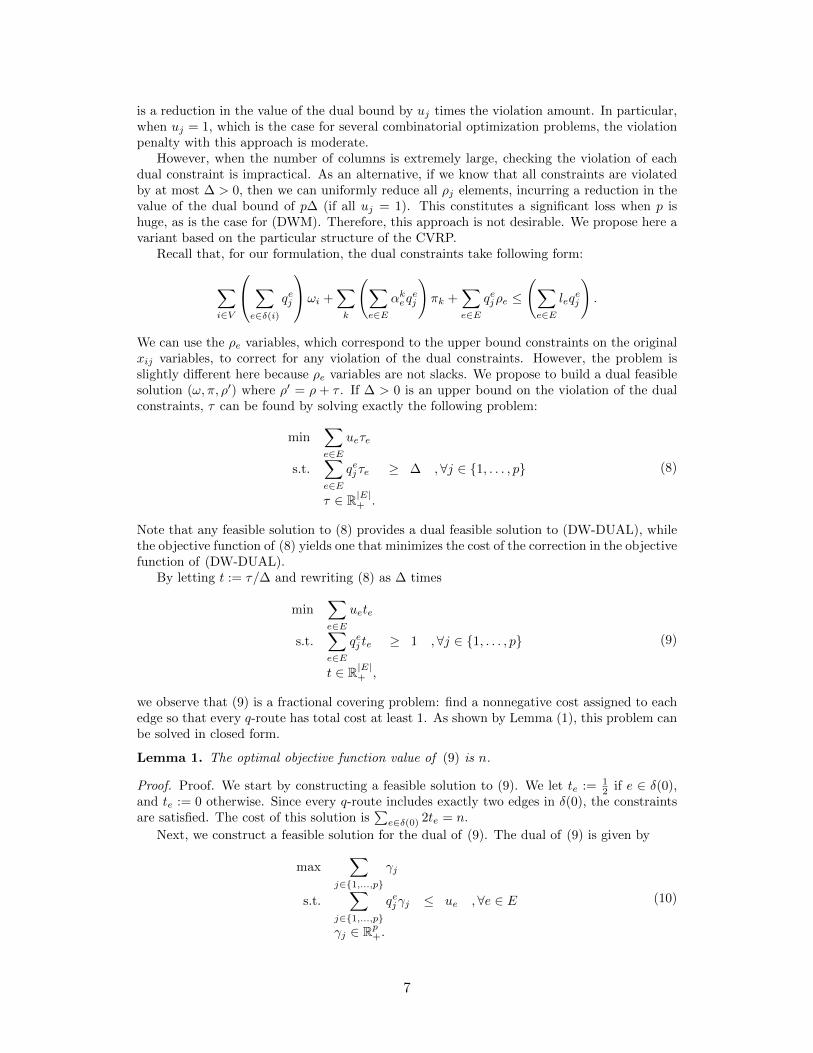
However, when the number of columns is extremely large, checking the violation of eachdual constraint is impractical. As an alternative, if we know that all constraints are violatedby at most ∆ > 0, then we can uniformly reduce all ρj elements, incurring a reduction in thevalue of the dual bound of p∆ (if all uj = 1). This constitutes a significant loss when p ishuge, as is the case for (DWM). Therefore, this approach is not desirable. We propose here avariant based on the particular structure of the CVRP.

Recall that, for our formulation, the dual constraints take following form:

∑i∈V

∑e∈δ(i)

qej

ωi +∑k

(∑e∈E

αkeqej

)πk +

∑e∈E

qejρe ≤

(∑e∈E

leqej

).

We can use the ρe variables, which correspond to the upper bound constraints on the originalxij variables, to correct for any violation of the dual constraints. However, the problem isslightly different here because ρe variables are not slacks. We propose to build a dual feasiblesolution (ω, π, ρ′) where ρ′ = ρ + τ . If ∆ > 0 is an upper bound on the violation of the dualconstraints, τ can be found by solving exactly the following problem:

min∑e∈E

ueτe

s.t.∑e∈E

qej τe ≥ ∆ ,∀j ∈ {1, . . . , p}

τ ∈ R|E|+ .

(8)

Note that any feasible solution to (8) provides a dual feasible solution to (DW-DUAL), whilethe objective function of (8) yields one that minimizes the cost of the correction in the objectivefunction of (DW-DUAL).

By letting t := τ/∆ and rewriting (8) as ∆ times

min∑e∈E

uete

s.t.∑e∈E

qej te ≥ 1 ,∀j ∈ {1, . . . , p}

t ∈ R|E|+ ,

(9)

we observe that (9) is a fractional covering problem: find a nonnegative cost assigned to eachedge so that every q-route has total cost at least 1. As shown by Lemma (1), this problem canbe solved in closed form.

Lemma 1. The optimal objective function value of (9) is n.

Proof. Proof. We start by constructing a feasible solution to (9). We let te := 12 if e ∈ δ(0),

and te := 0 otherwise. Since every q-route includes exactly two edges in δ(0), the constraintsare satisfied. The cost of this solution is

∑e∈δ(0) 2te = n.

Next, we construct a feasible solution for the dual of (9). The dual of (9) is given by

max∑

j∈{1,...,p}

γj

s.t.∑

j∈{1,...,p}

qejγj ≤ ue ,∀e ∈ E

γj ∈ Rp+.

(10)

7

The optimization problem (10) is fractional packing problem: assign costs to each q-routesuch that the total cost of any edge is at most ue. We set γj := 1 if route j goes from thedepot to some node i and immediately back to the depot. There are exactly n such q-routes.Otherwise, γj := 0. For an edge e /∈ δ(0), the left-hand side of the constraint will be zero. Foran edge e ∈ δ(0), we have ue = 0, and exactly two q-routes with γj = 1 will use that edge,yielding

∑j∈{1,...,p} q

ejγj = 2 ≤ ue.

We now have a primal feasible solution and a dual feasible solution to (9) with value n.By strong duality, those solutions are optimal.

We can thus construct a feasible (and optimal) solution to (8) with value n∆, which leadsto the following proposition.

Proposition 2. Let (ω, π, ρ) ∈ RV × Rκ+ × RE− and let ∆ > 0 be the largest violation of anyconstraint of (DW-DUAL) by (ω, π, ρ).

Then, (∑i∈V

biωi +∑k∈κ

αk0 πk +∑e∈E

ueρe

)− n∆ (11)

is a valid lower bound for (DWM).

3.2.1 Tightening the bound in (11):

By analyzing the dynamic programming algorithm in a bit more detail, one slightly tighterlower bound is obtained through the following refinement. Recall that in (6), we defined∆e := −minj:qej≥1{sj}, for all e ∈ δ(0). That is, ∆e is the largest violation of any dualconstraint corresponding to a q-route that includes the edge e.

We now have a relaxed version of (8), that describes exactly the problem of finding aminimal cost corrector τ

min∑e∈E

ueτe

s.t.∑e∈E

qej τe ≥ −sj ,∀j ∈ {1, . . . , p}

τ ∈ R|E|+ .

(12)

Guided by Lemma 1, we derive the following result:

Lemma 2. There exists a feasible solution to (12) with objective function value∑e∈δ(0) ∆e.

Proof. Proof. We construct a feasible solution to (12) by letting τe := 12∆e if e ∈ δ(0), and

τe := 0 otherwise. For all j, the left-hand side of the constraints becomes∑e∈δ(0)

qej1

2∆e =

1

2

(∆d + ∆f

),

for some d, f ∈ δ(0) such that d 6= f and qdj = qfj = 1, or d = f and qdj = qfj = 2. Using thedefinition of ∆e, we get

1

2

(∆d + ∆f

)=

1

2

(− mink:qdk≥1

{sk} − mink:qfj≥1

{sk}

)≥ 1

2(−sj − sj) = −sj ,

showing the feasibility of the solution τ . Its cost is∑e∈δ(0) ue

12∆e =

∑e∈δ(0) ∆e.

This leads to the following proposition.

8

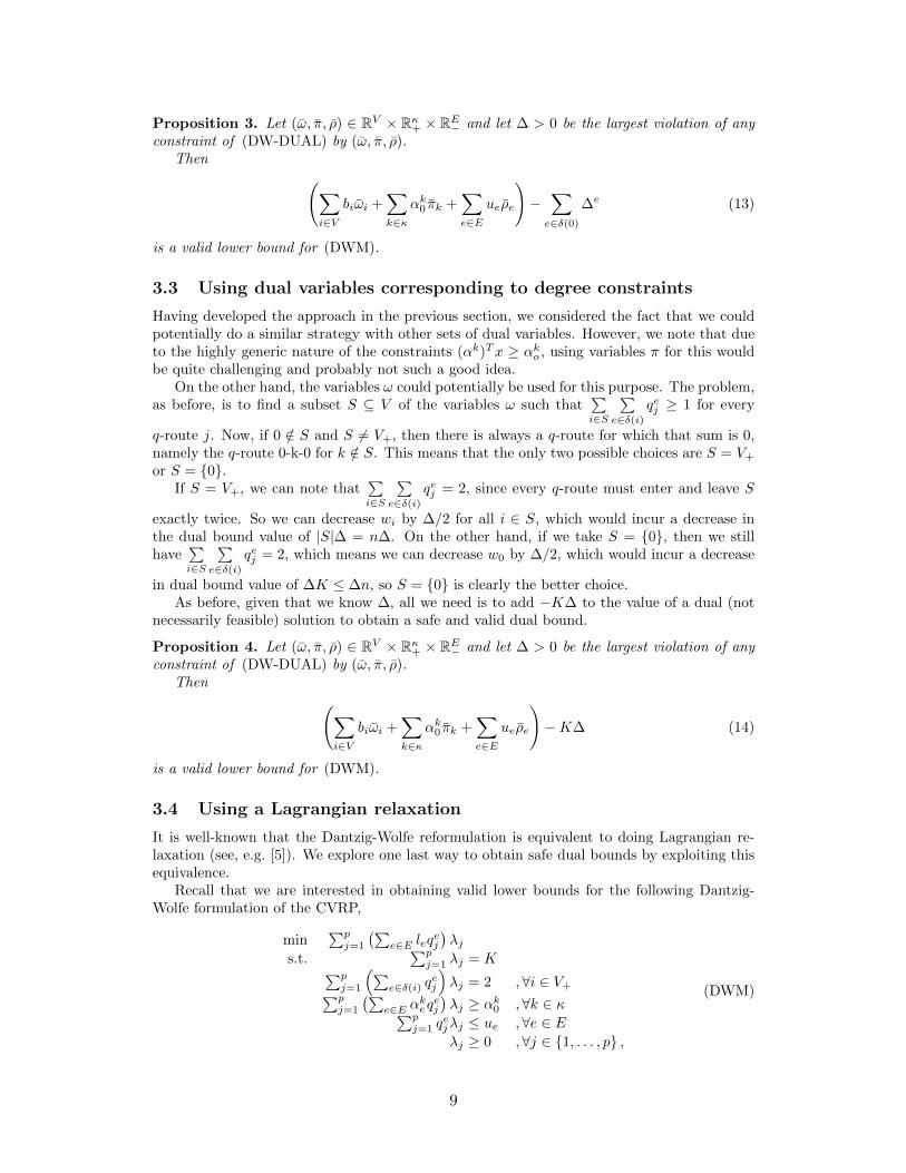
Proposition 3. Let (ω, π, ρ) ∈ RV × Rκ+ × RE− and let ∆ > 0 be the largest violation of anyconstraint of (DW-DUAL) by (ω, π, ρ).

Then (∑i∈V

biωi +∑k∈κ

αk0 πk +∑e∈E

ueρe

)−∑e∈δ(0)

∆e (13)

is a valid lower bound for (DWM).

3.3 Using dual variables corresponding to degree constraints

Having developed the approach in the previous section, we considered the fact that we couldpotentially do a similar strategy with other sets of dual variables. However, we note that dueto the highly generic nature of the constraints (αk)Tx ≥ αko , using variables π for this wouldbe quite challenging and probably not such a good idea.

On the other hand, the variables ω could potentially be used for this purpose. The problem,as before, is to find a subset S ⊆ V of the variables ω such that

∑i∈S

∑e∈δ(i)

qej ≥ 1 for every

q-route j. Now, if 0 /∈ S and S 6= V+, then there is always a q-route for which that sum is 0,namely the q-route 0-k-0 for k /∈ S. This means that the only two possible choices are S = V+

or S = {0}.If S = V+, we can note that

∑i∈S

∑e∈δ(i)

qej = 2, since every q-route must enter and leave S

exactly twice. So we can decrease wi by ∆/2 for all i ∈ S, which would incur a decrease inthe dual bound value of |S|∆ = n∆. On the other hand, if we take S = {0}, then we stillhave

∑i∈S

∑e∈δ(i)

qej = 2, which means we can decrease w0 by ∆/2, which would incur a decrease

in dual bound value of ∆K ≤ ∆n, so S = {0} is clearly the better choice.As before, given that we know ∆, all we need is to add −K∆ to the value of a dual (not

necessarily feasible) solution to obtain a safe and valid dual bound.

Proposition 4. Let (ω, π, ρ) ∈ RV × Rκ+ × RE− and let ∆ > 0 be the largest violation of anyconstraint of (DW-DUAL) by (ω, π, ρ).

Then (∑i∈V

biωi +∑k∈κ

αk0 πk +∑e∈E

ueρe

)−K∆ (14)

is a valid lower bound for (DWM).

3.4 Using a Lagrangian relaxation

It is well-known that the Dantzig-Wolfe reformulation is equivalent to doing Lagrangian re-laxation (see, e.g. [5]). We explore one last way to obtain safe dual bounds by exploiting thisequivalence.

Recall that we are interested in obtaining valid lower bounds for the following Dantzig-Wolfe formulation of the CVRP,

min∑pj=1

(∑e∈E leq

ej

)λj

s.t.∑pj=1 λj = K∑p

j=1

(∑e∈δ(i) q

ej

)λj = 2 ,∀i ∈ V+∑p

j=1

(∑e∈E α

keqej

)λj ≥ αk0 ,∀k ∈ κ∑p

j=1 qejλj ≤ ue ,∀e ∈ Eλj ≥ 0 ,∀j ∈ {1, . . . , p} ,

(DWM)

9

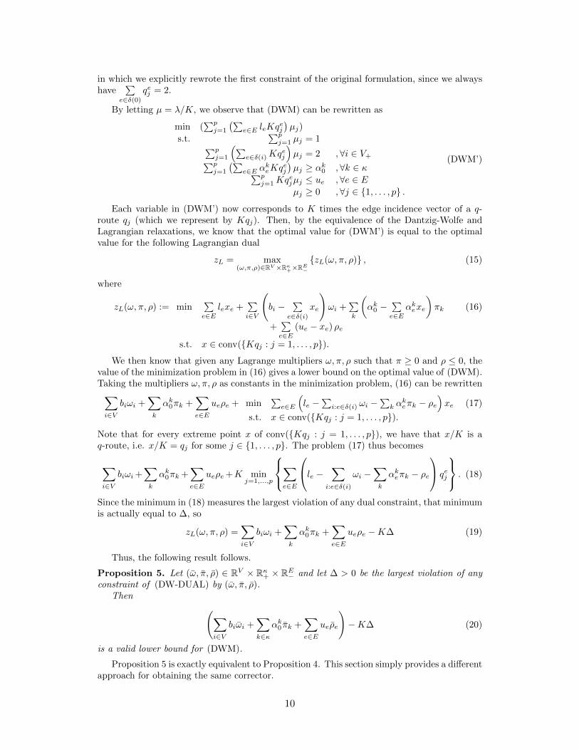
in which we explicitly rewrote the first constraint of the original formulation, since we alwayshave

∑e∈δ(0)

qej = 2.

By letting µ = λ/K, we observe that (DWM) can be rewritten as

min (∑pj=1

(∑e∈E leKq

ej

)µj)

s.t.∑pj=1 µj = 1∑p

j=1

(∑e∈δ(i)Kq

ej

)µj = 2 ,∀i ∈ V+∑p

j=1

(∑e∈E α

keKq

ej

)µj ≥ αk0 ,∀k ∈ κ∑p

j=1Kqejµj ≤ ue ,∀e ∈ Eµj ≥ 0 ,∀j ∈ {1, . . . , p} .

(DWM’)

Each variable in (DWM’) now corresponds to K times the edge incidence vector of a q-route qj (which we represent by Kqj). Then, by the equivalence of the Dantzig-Wolfe andLagrangian relaxations, we know that the optimal value for (DWM’) is equal to the optimalvalue for the following Lagrangian dual

zL = max(ω,π,ρ)∈RV ×Rκ+×RE−

{zL(ω, π, ρ)} , (15)

where

zL(ω, π, ρ) := min∑e∈E

lexe +∑i∈V

(bi −

∑e∈δ(i)

xe

)ωi +

∑k

(αk0 −

∑e∈E

αkexe

)πk

+∑e∈E

(ue − xe) ρe

s.t. x ∈ conv({Kqj : j = 1, . . . , p}).

(16)

We then know that given any Lagrange multipliers ω, π, ρ such that π ≥ 0 and ρ ≤ 0, thevalue of the minimization problem in (16) gives a lower bound on the optimal value of (DWM).Taking the multipliers ω, π, ρ as constants in the minimization problem, (16) can be rewritten∑i∈V

biωi +∑k

αk0πk +∑e∈E

ueρe + min∑e∈E

(le −

∑i:e∈δ(i) ωi −

∑k α

keπk − ρe

)xe

s.t. x ∈ conv({Kqj : j = 1, . . . , p}).(17)

Note that for every extreme point x of conv({Kqj : j = 1, . . . , p}), we have that x/K is aq-route, i.e. x/K = qj for some j ∈ {1, . . . , p}. The problem (17) thus becomes

∑i∈V

biωi+∑k

αk0πk +∑e∈E

ueρe+K minj=1,...,p

∑e∈E

le − ∑i:e∈δ(i)

ωi −∑k

αkeπk − ρe

qej

. (18)

Since the minimum in (18) measures the largest violation of any dual constraint, that minimumis actually equal to ∆, so

zL(ω, π, ρ) =∑i∈V

biωi +∑k

αk0πk +∑e∈E

ueρe −K∆ (19)

Thus, the following result follows.

Proposition 5. Let (ω, π, ρ) ∈ RV × Rκ+ × RE− and let ∆ > 0 be the largest violation of anyconstraint of (DW-DUAL) by (ω, π, ρ).

Then (∑i∈V

biωi +∑k∈κ

αk0 πk +∑e∈E

ueρe

)−K∆ (20)

is a valid lower bound for (DWM).

Proposition 5 is exactly equivalent to Proposition 4. This section simply provides a differentapproach for obtaining the same corrector.

10

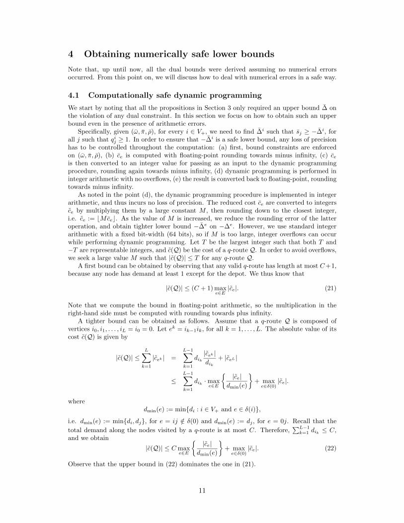
4 Obtaining numerically safe lower bounds

Note that, up until now, all the dual bounds were derived assuming no numerical errorsoccurred. From this point on, we will discuss how to deal with numerical errors in a safe way.

4.1 Computationally safe dynamic programming

We start by noting that all the propositions in Section 3 only required an upper bound ∆ onthe violation of any dual constraint. In this section we focus on how to obtain such an upperbound even in the presence of arithmetic errors.

Specifically, given (ω, π, ρ), for every i ∈ V+, we need to find ∆i such that sj ≥ −∆i, forall j such that qij ≥ 1. In order to ensure that −∆i is a safe lower bound, any loss of precisionhas to be controlled throughout the computation: (a) first, bound constraints are enforcedon (ω, π, ρ), (b) ce is computed with floating-point rounding towards minus infinity, (c) ceis then converted to an integer value for passing as an input to the dynamic programmingprocedure, rounding again towards minus infinity, (d) dynamic programming is performed ininteger arithmetic with no overflows, (e) the result is converted back to floating-point, roundingtowards minus infinity.

As noted in the point (d), the dynamic programming procedure is implemented in integerarithmetic, and thus incurs no loss of precision. The reduced cost ce are converted to integersce by multiplying them by a large constant M , then rounding down to the closest integer,i.e. ce := bMcec. As the value of M is increased, we reduce the rounding error of the latteroperation, and obtain tighter lower bound −∆e on −∆e. However, we use standard integerarithmetic with a fixed bit-width (64 bits), so if M is too large, integer overflows can occurwhile performing dynamic programming. Let T be the largest integer such that both T and−T are representable integers, and c(Q) be the cost of a q-route Q. In order to avoid overflows,we seek a large value M such that |c(Q)| ≤ T for any q-route Q.

A first bound can be obtained by observing that any valid q-route has length at most C+1,because any node has demand at least 1 except for the depot. We thus know that

|c(Q)| ≤ (C + 1) maxe∈E|ce|. (21)

Note that we compute the bound in floating-point arithmetic, so the multiplication in theright-hand side must be computed with rounding towards plus infinity.

A tighter bound can be obtained as follows. Assume that a q-route Q is composed ofvertices i0, i1, . . . , iL = i0 = 0. Let ek = ik−1ik, for all k = 1, . . . , L. The absolute value of itscost c(Q) is given by

|c(Q)| ≤L∑k=1

|cek | =

L−1∑k=1

dik|cek |dik

+ |ceL |

≤L−1∑k=1

dik ·maxe∈E

{|ce|

dmin(e)

}+ maxe∈δ(0)

|ce|.

wheredmin(e) := min{di : i ∈ V+ and e ∈ δ(i)},

i.e. dmin(e) := min{di, dj}, for e = ij /∈ δ(0) and dmin(e) := dj , for e = 0j. Recall that the

total demand along the nodes visited by a q-route is at most C. Therefore,∑L−1k=1 dik ≤ C,

and we obtain

|c(Q)| ≤ C maxe∈E

{|ce|

dmin(e)

}+ maxe∈δ(0)

|ce|. (22)

Observe that the upper bound in (22) dominates the one in (21).

11

Taking into account that |bλc| < |λ|+ 1 for all λ ∈ R, and that dmin(e) ≥ 1 for all e ∈ E,we replace ce with bMcec to obtain the expression

|c(Q,M)| ≤ C maxe∈E

{|bMcec|dmin(e)

}+ maxe∈δ−(0)

|bMcec|

≤ C maxe∈E

{M |ce|+ 1

dmin(e)

}+ maxe∈δ−(0)

(M |ce|+ 1)

≤ C

(M max

e∈E

{|ce|

dmin(e)

}+ 1

)+M max

e∈δ−(0)|ce|+ 1

≤ CM maxe∈E

{|ce|

dmin(e)

}+M max

e∈δ−(0)|ce|+ C + 1 ≤ T.

It is thus safe to choose any M such that

M ≤ (T − C − 1)/

(C max

e∈E

{|ce|

dmin(e)

}+ maxe∈δ−(0)

|ce|). (23)

By computing M under the appropriate rounding modes (rounding up all operations onthe denominator of the fraction and rounding down all other operations), one can guaranteethe validity of such upper bound, even with FP arithmetic.

4.2 Tying it all together

The first immediate use of the correctors described in Propositions 1, 2, 3, 4 and 5 is, aspreviously stated, to compute numerically safe lower bounds for (DWM).

In order to do so, we use a numerically safe upper bound ∆ as described in Section 4.1in place of ∆. Then, for individual arithmetic operations, we make sure to obtain appropri-ate bounds on the result: upper bounds if that result is subtracted or is in a denominator;lower bounds bounds otherwise. This is achieved by controlling the “rounding mode” of theprocessor, as detailed below in Section 4.3.

For example, to compute the bound (7), we first compute an upper bound on 2lf + ∆

by rounding errors up on the sum, then compute the lower bound on2lf

2lf+∆by performing

the division while rounding errors down, and finally do all remaining sums and multiplicationrounding down. In the end, we get a value guaranteed to be lower than the value in (7) andhence still a valid lower bound for (DWM). We refrain from detailing how safe bounds can becomputed for all other propositions, since the operations are analogous. Using this approach,each of those bounds is easily computable in a numerically safe way to ensure it is valid,regardless of arithmetic errors.

In addition, there are other potential advantages to using those propositions. One well-known issue when dealing with column generation-type algorithms is dealing with tolerancesto determine when the column generation process has converged. If these tolerances are notchosen well enough, one may end up with a suboptimal solution to (DWM) and thus withan invalid lower bound for the current node of the branch-and-bound tree. Furthermore, onemay also be faced with cycling, a situation in which the pricing algorithm concludes that somecolumns have a negative reduced cost, but the LP solver decides that they should not enter thebasis, due to rounding errors or tolerances. Then, the LP solver will not make any iterationand thus not change the dual variables, yielding exactly the same columns to be generated overand over. These issues create the need for a careful calibration of column generation tolerances,in conjunction with the tolerances of the LP solver. However, with the Propositions 1-5 inhand, one can simply abort column generation at any point and still get a valid dual bound,regardless of whether true convergence is attained.

This last point can be exploited even further and used to our advantage within a branch-and-bound context. For instance, even without the issues of tolerances, when performing

12

column generation, we need to wait until convergence occurs to be able to obtain a valid dualbound. However, it is often the case that the initial column generation iterations are verycheap (as they are usually performed by fast heuristics) and the final ones are more expensive.Therefore, if we can avoid the final column generation iterations, we would be able to savesome time. In particular, if we compute the dual bound proposed in Propositions 1-5 and ittells us that the current node can be pruned, we can exit early; we do not need to run columngeneration until full convergence.

4.3 Implementation details

The result of an operation in floating-point arithmetic may not be representable in the chosenfloating-point format, in our case 64-bits IEEE-754 double precision ([19]). Then, it is roundedto a nearby representable number. By default, it is rounded to the nearest representablefloating-point value, which could be smaller or larger. But in order to perform safe arithmetic,we need to control the direction of the rounding. For example, we obtain safe lower boundsby always rounding towards minus infinity. Since C99, the standard C library provides afunction fesetround() to change the rounding mode for the current thread ([22]). However,the support for changing the rounding mode is absent in LLVM ([25], as of version 3.5.0), andexperimental in GCC (as of version 4.9.2). Specifically, the optimizer pass of GCC is not awarethat the rounding mode can be changed. It thus allows arithmetic operations to be reorderedaround calls to fesetround() and other functions affecting floating-point arithmetic ([16, 15]).For instance, the following two snippets of code may (and, in our experience, will) compileinto the same assembly output:

fesetround(FE DOWNWARD);

x = 1.0 / a;

fesetround(FE TONEAREST);

y = 1.0 / a;

fesetround(FE DOWNWARD);

fesetround(FE TONEAREST);

x = 1.0 / a;

y = 1.0 / a;

To the best of our knowledge, there is no reliable way to impose an ordering on arithmeticoperations to the compiler. However, there exist a variety of tools to enforce an ordering onmemory access. For instance, the following code

fesetround(FE DOWNWARD);

compute x and y();

fesetround(FE TONEAREST);

behaves as expected as long as the function compute x and y() is defined in a different com-pilation unit (thus does not risk being inlined). Indeed, the compiler must preserve thecall order, in case compute x and y() accesses memory that depends on the side effects offesetround(FE DOWNWARD), or in case fesetround(FE TONEAREST) has a dependency on theside effects of compute x and y(). Since this method introduces the inconvenient need for hav-ing related code spread over different files, we describe several workarounds in Appendix A.

5 Computational experiments

Our code is based on the existing CVRP solver developed in [14], to which we added thesafe bound computing methods described in Section 3. The only major modification to theprevious code concerns the dynamic programming procedure. As noted in Section 4.1, weneed dynamic programming to return exact results for an integer input. Consequently, thedynamic programming code was rewritten to use standard 64-bit integers in all computations.The linear programming problems are solved using CPLEX 12.6.

13

We present four different experiments. The first is intended to verify whether the new im-plementation of a safe dynamic programming procedure introduces any performance penalty.The second evaluates potential performance gains arising from the use of safe bounds. Thethird compares safe bounds with their unsafe counterparts, and tests whether unsafe or inef-ficient branching/pruning decisions were taken by the unsafe code. The fourth compares thestrength of the three different bounds developed in Section 3.

5.1 Performance of safe dynamic programming

The dynamic programming routine implements the method from [21] for finding shortest q-routes, with elimination of short cycles. A traditional variant of the code uses floating pointnumbers for edge costs, and a safe variant uses integers. Two additional steps are necessary inits safe variant: conversion of the input edge costs from floating-point into integers, and theconversion the output q-route lengths from integer into floating-point values. In this section,we measure whether those conversions or the use of integers in computations presents anyoverhead. Both variants are run on an Intel Core i5 3210M processor with 8Gb of memory.The compiler is GCC 4.9.2 and the OS kernel is Linux 3.19.5. For this test, we use the sameinstances as [14], but limit to problems with less than 50 clients. This decision was madefor practical reasons: we measure running times in this test, and running several instances inparallel would affect the accuracy of the measurements.

The results are presented in Table 1. Columns cols and time represent the total numberof columns generated across all nodes of the BCP algorithm and the total running time, foreither the safe or the unsafe/traditional variant of the code. The geometric means are reportedfor each column over all instances in the table. For some instances, we observe large variationsbetween the two variants, both in number of columns generated and in running time. Thisis not surprising since slightly different solution paths may induce branch-and-bound trees ofwidely varying sizes. However, the numbers are very similar for most instances. In geometricmean, the safe code lead to the generation of 1051.1 columns per instance, while the unsafecode involved 1026.8 columns. The associated running times, also in geometric mean, are5.008 seconds and 4.154 seconds, respectively. While it appears that the safe code is slightlyslower on average, the difference in computational cost is certainly not prohibitive.

5.2 Safe bounds and column generation

The test in the previous section measures the compound effect of two differences between thesafe and unsafe variants of our code. On the one hand, the safe variant has some overhead. Onthe other hand, as mentioned in Section 4.2, safe bounds let us interrupt column generationearlier in some cases. The test in this section intends to determine the effect of the latter. Itis performed on the same computer and with the same instances as the previous test, and itsresults are shown in Table 2.

Here, whenever we determine that column generation could be interrupted early (i.e. beforeconvergence), we start a timer and proceed until convergence is obtained. This way, we obtainan estimation of how many columns and how much time would be spared by interruptingcolumn generation early, represented in the second and fourth columns of Table 2, respectively.Note that this is only an estimation, since columns that are avoided by early interruption maybe needed later in other nodes of the branch-and-bound tree.

Note that in this experiment, column generation is interrupted only when the safe boundguarantees that the current node can be pruned. Our technique could let us stop the procedureat any earlier point with a valid (yet weaker) bound, in order to compute branch-and-boundnodes faster, at the risk of evaluating more nodes. However, this would require further finetuning of our branch-and-cut-and-price framework, and is beyond the scope of this paper.

We observe that the early-exit strategy lets us avoid generating some columns in almostall instances. But the computing time associated with generating those columns remainsmarginal, around 1% for most instances. This is consistent with the corresponding gains in

14

safe unsafe safe unsafeInstance nBB cols time (s) nBB cols time (s) Instance nBB cols time (s) nBB cols time (s)A-n32-k5 1 817 0.405 1 819 0.378 B-n43-k6 13 1611 26.625 12 1858 30.614A-n33-k5 1 715 0.303 1 715 0.251 B-n44-k7 1 1552 0.965 1 1634 1.049A-n33-k6 5 666 6.721 4 695 4.434 B-n45-k5 7 2609 103.405 4 2545 69.317A-n34-k5 3 949 3.627 3 943 3.152 B-n45-k6 5 1828 15.819 4 1847 14.720A-n36-k5 11 1379 38.002 7 1197 15.279 E-n13-k4 1 51 0.027 1 51 0.012A-n37-k5 32 3199 116.026 6 1668 29.394 E-n22-k4 1 240 0.088 1 240 0.073A-n37-k6 50 1420 58.441 76 2673 93.742 E-n23-k3 1 925 5.029 1 943 5.576A-n38-k5 19 2432 62.683 18 2760 55.337 E-n30-k3 1 2668 2.773 1 2583 2.915A-n39-k5 7 1627 18.813 7 1668 17.514 E-n31-k7 3 631 3.045 3 619 3.067A-n39-k6 9 1643 19.781 9 1480 19.069 E-n33-k4 1 1556 3.602 1 1534 3.555A-n44-k6 3 1136 7.678 3 1126 6.903 F-n45-k4 1 6421 47.302 1 5840 39.677A-n45-k6 70 3837 293.958 55 3426 176.184 P-n16-k8 4 65 0.170 4 65 0.167A-n45-k7 50 2300 94.880 72 3563 154.411 P-n19-k2 1 506 0.231 1 506 0.228A-n46-k7 2 1531 5.600 2 1572 11.525 P-n20-k2 3 625 4.113 3 592 4.065A-n48-k7 168 5803 549.395 25 1733 60.152 P-n21-k2 1 520 0.227 1 520 0.269B-n31-k5 1 1013 0.448 1 1013 0.400 P-n22-k2 2 615 5.369 2 615 5.344B-n34-k5 14 1471 34.509 14 1298 39.387 P-n22-k8 1 109 0.039 1 109 0.027B-n35-k5 1 1593 0.635 1 1655 0.623 P-n23-k8 1 143 0.032 1 143 0.029B-n38-k6 7 1303 19.619 7 1284 19.590 P-n40-k5 2 1300 9.234 2 1300 9.194B-n39-k5 2 2099 10.955 1 1978 1.271 P-n45-k5 21 1939 105.038 26 2367 177.198B-n41-k6 3 1513 11.111 3 1452 12.186

geom. mean 3.8 1051.1 5.008 3.4 1026.8 4.154

Table 1: Computing time for safe and unsafe DP

the safe code being insufficient to compensate for the overhead, in Table 1. However, Table 2confirms that the technique is useful in practice, although not much.

5.3 Safe bounds and unsafe bounds

The primary aim of this paper is to ensure that the pruning of branch-and-bound nodes isperformed safely, i.e. without any risk of improper pruning, and without the need for arbitrarytolerances. We now examine the safe lower bounds that we obtain, in comparison to the unsafebounds previously used in the code.

In order to obtain a fair comparison, for every branch-and-bound node, we first compute abound zu in floating-point arithmetic, then use the safe variant of the code to compute a safebound zs. For zu, as is standard practice, a small value ε is subtracted from the LP boundcomputed in FP arithmetic, to account for FP rounding errors. For the safe bound, we usethe maximum (i.e. strongest) of the safe bounds developed in Propositions 1-5.

In Table 3, we count for each of zs and zu, in how many nodes the bound was stronger. Webreak ties in favor of the unsafe bound since, as the safe bound incurs an overhead, we wantto understand when our method is strictly preferable. Therefore, the number represented inthe zs column represents the number of nodes for which zs > zu, and the number in the zu

column represents the number of nodes for which zs ≤ zu. The column “nBB” denotes thetotal number of branch-and-bound nodes. In the first group of columns, zu is computed usinga threshold of ε = 10−6, the value used by [14]. In the second group of columns, zu is computedwith ε = 10−9, in order to illustrate the importance of the choice of ε in an unsafe code. Insome cases, the difference between zs and zu is large enough to result in different branchingdecisions being taken depending on which is used as a bound. If that is the case with zs > zu,it means that the unsafe code performed unnecessary branching. If it happens with zu ≥ zs,the unsafe code might have performed unsafe pruning, although it may also be explained bythe safe bound being too weak. The number of branch-and-bound nodes for which such eventoccurred is indicated between parenthesis when it is not zero.

The test was run on a computer with 48 AMD Opteron 6176 processor cores and 256Gbof memory. The compiler is GCC 4.4.7 and the OS kernel is Linux 2.6.32. For this test,

15

total late total late total late total lateInstance cols cols time (s) time (s) Instance cols cols time (s) time (s)A-n32-k5 817 4 0.400 0.010 B-n43-k6 1611 336 26.322 0.932A-n33-k5 715 0.301 B-n44-k7 1552 4 0.902 0.017A-n33-k6 666 22 4.764 0.046 B-n45-k5 2609 145 93.644 0.601A-n34-k5 949 22 3.662 0.072 B-n45-k6 1888 120 15.457 0.411A-n36-k5 1610 48 46.791 0.189 E-n13-k4 51 0.024A-n37-k5 1614 98 18.500 0.289 E-n22-k4 240 0.073A-n37-k6 1391 383 56.109 0.963 E-n23-k3 925 5.042A-n38-k5 2445 161 50.018 0.460 E-n30-k3 2668 35 2.777 0.111A-n39-k5 1627 167 18.162 0.314 E-n31-k7 631 16 3.031 0.043A-n39-k6 1643 81 18.605 0.237 E-n33-k4 1556 10 3.403 0.204A-n44-k6 1136 24 7.160 0.099 F-n45-k4 6421 35 45.725 1.526A-n45-k6 3091 367 229.066 1.771 P-n16-k8 65 0.121A-n45-k7 2282 528 78.265 1.702 P-n19-k2 506 0.281A-n46-k7 1531 29 5.408 0.097 P-n20-k2 625 27 4.015 0.044A-n48-k7 5049 1465 416.991 6.209 P-n21-k2 520 0.205B-n31-k5 1013 11 0.393 0.019 P-n22-k2 615 21 5.250 0.044B-n34-k5 1484 189 34.382 0.470 P-n22-k8 109 0.028B-n35-k5 1593 0.601 P-n23-k8 143 0.024B-n38-k6 1428 212 23.984 0.521 P-n40-k5 1300 84 8.634 0.220B-n39-k5 2099 46 10.816 0.120 P-n45-k5 1952 574 116.066 2.342B-n41-k6 1513 39 10.731 0.135

Table 2: Early-exit in column generation

we use all the instances from [14]. Some instances did not terminate within 500 hours:F-n135-k7.vrp, M-n200-k16.vrp, M-n200-k17.vrp, while others exhaust the available mem-ory: B-n50-k8.vrp, B-n64-k9.vrp, B-n78-k10.vrp, E-n101-k8.vrp, M-n151-k12.vrp. Par-tial results are reported for those instances, on the branch-and-bound nodes that were pro-cessed.

Our results indicate that zs is stronger than the zu in the overwhelming majority of thenodes, despite being a safe bound. This is the case even when zu is computed with thedangerously small tolerance ε = 10−9. However, in our tests, the difference between zs andzu was never large enough to let the safe code prune nodes that the unsafe code could notprune. It must be noted that the objective function of most instances is integer, or can bemade integer by multiplying it by a small power of ten. As a consequence, most LP boundscan be rounded up before being compared to the incumbent solution, rendering small errorsharmless whenever the LP bound is far from an integral value.

On the other hand, with ε = 10−6, zu was rarely stronger than zs, and also never ledto the unsafe code performing dangerous pruning. It is thus unlikely that the optimality ofsolutions reported in [14] is affected by FP errors. The conclusions differ for ε = 10−9 however,with unsafe pruning occurring in four distinct instances (A-n60-k9, B-n68-k9, B-n78-k10,M-n121-k7). This tends to validate the choice of 10−6 for ε.

5.4 Comparison of safe bounds

In this section, we compare the bound correctors developed in Section 3. We reuse the datagenerated in the experiment of the previous section, but this time count for the number ofnodes in which each was the strongest. Table 4 shows such numbers. Again, “nBB” denotesthe total number of branch-and-bound nodes. We denote by zrho the bound resulting fromProposition 3, by zsc the one from Proposition 1, and by zLag the one from Propositions 5and 4. Whenever a bound is strictly stronger than the others for a number of nodes, that

16

ε = 10−6 ε = 10−9 ε = 10−6 ε = 10−9

Instance nBB zs zu zs zu Instance nBB zs zu zs zu

A-n32-k5 0 0 0 0 0 B-n68-k9 4428 4428 0 4345 83 (1)A-n33-k5 0 0 0 0 0 B-n78-k10 3449 3449 0 3185 264 (4)A-n33-k6 3 3 0 3 0 E-n101-k14 4331 4329 2 4247 84A-n34-k5 4 4 0 4 0 E-n101-k8 3190 3177 13 3088 102A-n36-k5 6 6 0 6 0 E-n13-k4 0 0 0 0 0A-n37-k5 4 4 0 4 0 E-n22-k4 0 0 0 0 0A-n37-k6 62 62 0 62 0 E-n23-k3 0 0 0 0 0A-n38-k5 30 30 0 30 0 E-n30-k3 0 0 0 0 0A-n39-k5 4 4 0 4 0 E-n31-k7 1 1 0 1 0A-n39-k6 8 8 0 8 0 E-n33-k4 0 0 0 0 0A-n44-k6 2 2 0 2 0 E-n51-k5 2 2 0 2 0A-n45-k6 10 10 0 10 0 E-n76-k10 1726 1726 0 1693 33A-n45-k7 59 59 0 59 0 E-n76-k14 4381 4381 0 4356 25A-n46-k7 1 1 0 1 0 E-n76-k7 1093 1092 1 1089 4A-n48-k7 165 165 0 160 5 E-n76-k8 311 311 0 301 10A-n53-k7 9 9 0 9 0 F-n135-k7 3 2 1 2 1A-n54-k7 45 45 0 44 1 F-n45-k4 0 0 0 0 0A-n55-k9 9 9 0 9 0 F-n72-k4 14 14 0 12 2A-n60-k9 615 615 0 600 15 (1) M-n101-k10 1 1 0 1 0A-n61-k9 174 174 0 166 8 M-n121-k7 70 69 1 59 11 (2)A-n62-k8 85 85 0 83 2 M-n151-k12 585 582 3 307 278A-n63-k10 377 377 0 370 7 M-n200-k16 58 58 0 6 52A-n63-k9 1083 1083 0 1035 48 M-n200-k17 554 550 4 94 460A-n64-k9 304 304 0 304 0 P-n101-k4 30 30 0 29 1A-n65-k9 10 10 0 10 0 P-n16-k8 3 3 0 3 0A-n69-k9 517 516 1 513 4 P-n19-k2 0 0 0 0 0A-n80-k10 84 84 0 80 4 P-n20-k2 2 2 0 2 0B-n31-k5 0 0 0 0 0 P-n21-k2 0 0 0 0 0B-n34-k5 10 10 0 10 0 P-n22-k2 1 1 0 1 0B-n35-k5 0 0 0 0 0 P-n22-k8 0 0 0 0 0B-n38-k6 3 3 0 3 0 P-n23-k8 0 0 0 0 0B-n39-k5 0 0 0 0 0 P-n40-k5 1 1 0 1 0B-n41-k6 2 2 0 2 0 P-n45-k5 23 23 0 23 0B-n43-k6 12 12 0 12 0 P-n50-k10 172 172 0 172 0B-n44-k7 0 0 0 0 0 P-n50-k7 4 4 0 4 0B-n45-k5 6 6 0 6 0 P-n50-k8 264 264 0 264 0B-n45-k6 2 2 0 2 0 P-n51-k10 22 22 0 22 0B-n50-k7 1 1 0 1 0 P-n55-k10 950 950 0 945 5B-n50-k8 10969 10968 1 10774 195 P-n55-k15 697 697 0 690 7B-n51-k7 214 214 0 214 0 P-n55-k7 1110 1110 0 1104 6B-n52-k7 8 8 0 8 0 P-n55-k8 104 104 0 104 0B-n56-k7 3 3 0 3 0 P-n60-k10 40 40 0 40 0B-n57-k7 11 11 0 10 1 P-n60-k15 20 20 0 20 0B-n57-k9 7 7 0 7 0 P-n65-k10 23 23 0 23 0B-n63-k10 14900 14895 5 14785 115 P-n70-k10 1475 1475 0 1447 28B-n64-k9 7998 7998 0 151 7847 P-n76-k4 85 84 1 77 8B-n66-k9 88 88 0 85 3 P-n76-k5 1670 1665 5 1645 25B-n67-k10 142 142 0 135 7

Table 3: Comparison of safe and unsafe bounds

17

number is indicated between parenthesis.As shown in Table 4, zsc was never strictly stronger than the other safe bounds in our

experiments. The strongest bound was most often zrho, but zLag was strictly stronger thanzrho in many cases. It is thus clear that none of zLag and zrho dominates the other. They areboth useful and complement each other in a safe code.

6 Conclusion

We propose several methods to obtain safe lower bounds for LP relaxations of the CapacitatedVehicle Routing Problem (CVRP). We then describe how these methods can be exploited inpractice. In particular, since we solve CVRP instances by column generation, we describe a safeimplementation of the dynamic programming procedure employed in the pricing step. Finally,we perform computations to compare the resulting bounds to those traditionally computedwith floating-point arithmetic and arbitrary tolerances. The first method is based on a scalingapproach proposed by [18] for graph coloring problems. However, the resulting bound is weakin practice. Three other methods are derived from ideas by [1] for the Travelling SalesmanProblem, and we adapt them to accommodate for column generation in the CVRP. The lastmethod is simply an alternate derivation of one of the bounds obtained previously, and isbased on a specific Lagrangian relaxation of the CVRP formulation.

In practice, the bounds obtained with our methods are in most cases stronger than thosecomputed with traditional floating-point arithmetic, in addition to being safe. Moreover, theycan be computed even when column generation has not converged yet. As a result, we caninterrupt column generation earlier in some cases. Our computations show that this techniqueyields a modest reduction in the cost of column generation, compensating in part for the smalloverhead of safe computations.

ACKNOWLEDGMENT: We would like to thank Laura Sanita and Ahmad Abdi for theirassistance with the problem (9).

References

[1] David Applegate, Robert E. Bixby, Vasek Chvatal, and William J. Cook. The TravelingSalesman Problem, A computational study. 2006.

[2] David Applegate, William J. Cook, Sanjeeb Dash, and Daniel Espinoza. Exact solutionsto linear programming problems. Operations Research Letters, 35(6):693–699, 2007.

[3] Roberto Baldacci, Aristide Mingozzi, and Roberto Roberti. New route relaxation andpricing strategies for the vehicle routing problem. Operations Research, 59(5):1269–1283,2011.

[4] Vasek Chvatal, William Cook, and Daniel Espinoza. Local cuts for mixed-integer pro-gramming. Mathematical Programming Computation, 5(2):171–200, 2013.

[5] Michele Conforti, Gerard Cornuejols, and Giacomo Zambelli. Integer Programming.Springer, 2014.

[6] Claudio Contardo and Rafael Martinelli. A new exact algorithm for the multi-depot vehi-cle routing problem under capacity and route length constraints. Discrete Optimization,12:129–146, 2014.

[7] William J. Cook, Sanjeeb Dash, Ricardo Fukasawa, and Marcos Goycoolea. Numericallysafe gomory mixed-integer cuts. INFORMS Journal of Computing, 21(4):641–649, 2009.

[8] William J. Cook, Thorsten Koch, Daniel Steffy, and Kati Wolter. An exact rationalmixed-integer programming solver. In Oktay Gunluk and Gerhard Woeginger, editors,IPCO, Lecture notes in computer science, volume 6655, pages 104–116, 2011.

18

zbest = zbest =Instance nBB zrho zsc zLag Instance nBB zrho zsc zLag

A-n32-k5 0 0 0 0 B-n68-k9 4428 (3806) 3857 0 (571) 622A-n33-k5 0 0 0 0 B-n78-k10 3449 (2991) 3000 0 (449) 458A-n33-k6 3 (1) 2 0 (1) 2 E-n101-k14 4331 (4152) 4162 0 (169) 179A-n34-k5 4 (1) 1 0 (3) 3 E-n101-k8 3190 (2077) 2080 1 (1110) 1113A-n36-k5 6 (3) 4 0 (2) 3 E-n13-k4 0 0 0 0A-n37-k5 4 (2) 2 0 (2) 2 E-n22-k4 0 0 0 0A-n37-k6 62 (29) 36 0 (26) 33 E-n23-k3 0 0 0 0A-n38-k5 30 (16) 20 0 (10) 14 E-n30-k3 0 0 0 0A-n39-k5 4 2 0 (2) 4 E-n31-k7 1 (1) 1 0 0A-n39-k6 8 (5) 7 0 (1) 3 E-n33-k4 0 0 0 0A-n44-k6 2 (1) 1 0 (1) 1 E-n51-k5 2 1 0 (1) 2A-n45-k6 10 (6) 7 0 (3) 4 E-n76-k10 1726 (1396) 1412 0 (314) 330A-n45-k7 59 (31) 37 0 (22) 28 E-n76-k14 4381 (4143) 4152 0 (229) 238A-n46-k7 1 (1) 1 0 0 E-n76-k7 1093 (705) 719 0 (374) 388A-n48-k7 165 (145) 151 0 (14) 20 E-n76-k8 311 (222) 234 0 (77) 89A-n53-k7 9 (5) 6 0 (3) 4 F-n135-k7 3 (1) 1 0 (2) 2A-n54-k7 45 (31) 40 1 (5) 14 F-n45-k4 0 0 0 0A-n55-k9 9 (4) 7 0 (2) 5 F-n72-k4 14 0 0 (14) 14A-n60-k9 615 (488) 493 0 (122) 127 M-n101-k10 1 (1) 1 0 0A-n61-k9 174 (145) 152 0 (22) 29 M-n121-k7 70 (33) 35 0 (35) 37A-n62-k8 85 (64) 69 0 (16) 21 M-n151-k12 585 (503) 504 0 (81) 82A-n63-k10 377 (299) 301 0 (76) 78 M-n200-k16 58 (54) 54 0 (4) 4A-n63-k9 1083 (937) 941 0 (142) 146 M-n200-k17 554 (538) 538 0 (16) 16A-n64-k9 304 (249) 255 1 (49) 55 P-n101-k4 30 (2) 2 0 (28) 28A-n65-k9 10 (8) 9 0 (1) 2 P-n16-k8 3 (1) 3 0 2A-n69-k9 517 (432) 443 0 (74) 85 P-n19-k2 0 0 0 0A-n80-k10 84 (75) 78 0 (6) 9 P-n20-k2 2 1 0 (1) 2B-n31-k5 0 0 0 0 P-n21-k2 0 0 0 0B-n34-k5 10 (3) 3 0 (7) 7 P-n22-k2 1 0 0 (1) 1B-n35-k5 0 0 0 0 P-n22-k8 0 0 0 0B-n38-k6 3 (2) 2 0 (1) 1 P-n23-k8 0 0 0 0B-n39-k5 0 0 0 0 P-n40-k5 1 0 0 (1) 1B-n41-k6 2 (2) 2 0 0 P-n45-k5 23 (15) 15 0 (8) 8B-n43-k6 12 (1) 4 0 (8) 11 P-n50-k10 172 (151) 164 0 (8) 21B-n44-k7 0 0 0 0 P-n50-k7 4 (2) 3 0 (1) 2B-n45-k5 6 (2) 2 0 (4) 4 P-n50-k8 264 (231) 242 1 (22) 33B-n45-k6 2 1 0 (1) 2 P-n51-k10 22 (20) 20 0 (2) 2B-n50-k7 1 0 0 (1) 1 P-n55-k10 950 (889) 916 0 (34) 61B-n50-k8 10969 (7821) 7898 1 (3071) 3148 P-n55-k15 697 (685) 691 0 (6) 12B-n51-k7 214 (137) 144 0 (70) 77 P-n55-k7 1110 (869) 900 0 (210) 241B-n52-k7 8 (4) 5 0 (3) 4 P-n55-k8 104 (83) 95 0 (9) 21B-n56-k7 3 (3) 3 0 0 P-n60-k10 40 (30) 36 0 (4) 10B-n57-k7 11 (8) 8 0 (3) 3 P-n60-k15 20 (12) 18 0 (2) 8B-n57-k9 7 (7) 7 0 0 P-n65-k10 23 (16) 19 0 (4) 7B-n63-k10 14900 (13908) 13977 0 (923) 992 P-n70-k10 1475 (1346) 1364 0 (111) 129B-n64-k9 7998 (7055) 7061 0 (937) 943 P-n76-k4 85 (13) 14 0 (71) 72B-n66-k9 88 (76) 76 0 (12) 12 P-n76-k5 1670 (669) 686 1 (984) 1001B-n67-k10 142 (115) 118 0 (24) 27

Table 4: Strongest safe bounds

19

[9] William J. Cook, Thorsten Koch, Daniel Steffy, and Kati Wolter. A hybrid branch-and-bound approach for exact rational mixed-integer programming. Mathematical Program-ming Computation, 5:305–344, 2013.

[10] Gerard Cornuejols, Francois Margot, and Giacomo Nannicini. On the safety of gomorycut generators. Mathematical Programming Computation, 5:345–395, 2013.

[11] George Dantzig and John Ramser. The truck dispatching problem. Management Science,6:80–91, 1959.

[12] Daniel G. Espinoza. On Linear Programming, Integer Programming and Cutting Planes.PhD thesis, School of Industrial and Systems Engineering, Georgia Institute of Technol-ogy, March 2006.

[13] Matteo Fischetti and Andrea Lodi. Local branching. Mathematical Programming, 98(1–3):23–47, 2003.

[14] Ricardo Fukasawa, Humberto Longo, Jens Lysgaard, Marcus Poggi de Aragao, MarceloReis, Eduardo Uchoa, and Renato F. Werneck. Robust branch-and-cut-and-price for thecapacitated vehicle routing problem. Mathematical Programming, 106(3):491–511, 2006.

[15] GCC Bugzilla. Optimization breaks floating point exception flag reading. Accessed April15, 2015. https://gcc.gnu.org/bugzilla/show_bug.cgi?id=29186, 2006.

[16] GCC Bugzilla. Optimization generates incorrect code with -frounding-math option. Ac-cessed April 15, 2015. https://gcc.gnu.org/bugzilla/show_bug.cgi?id=34678, 2008.

[17] David Goldberg. What every computer scientist should know about floating-point arith-metic. ACM Computing Surveys (CSUR), 23(1):5–48, 1991.

[18] Stephan Held, William J. Cook, and Edward C. Sewell. Maximum-weight stable sets andsafe lower bounds for graph coloring. Mathematical Programming Computation, 4:363–381, 2012.

[19] IEEE. IEEE standard for binary floating-point arithmetic. Institute of Electrical andElectronics Engineers, New York, 1985. Standard 754–1985.

[20] IBM ILOG. CPLEX 12.6, 2013. http://www.ilog.com/products/cplex.

[21] Stefan Irnich and Daniel Villeneuve. The shortest-path problem with resource constraintsand k-cycle elimination for k ≥ 3. INFORMS Journal on Computing, 18(3):391–406,January 2006.

[22] ISO/IEC. Programming languages – C. International Organization for Standardization,1999. Standard ISO/IEC 9899:1999.

[23] Thorsten Koch, Tobias Achterberg, Erling Andersen, Oliver Bastert, Timo Berthold,Robert E. Bixby, Emilie Danna, Gerald Gamrath, Ambros M. Gleixner, Stefan Heinz,Andrea Lodi, Hans Mittelmann, Ted Ralphs, Domenico Salvagnin, Daniel E. Steffy, andKati Wolter. MIPLIB 2010. Mathematical Programming Computation, 3(2):103–163,2011.

[24] Adam Letchford, Richard Eglese, and Jens Lysgaard. Multistars, partial multistars andthe capacitated vehicle routing problem. Mathematical Programming, 94:21–40, 2002.

[25] LLVM Bugzilla. Clang/LLVM don’t support C99 FP rounding mode pragmas. AccessedMay 24, 2015. https://llvm.org/bugs/show_bug.cgi?id=8100, 2010.

[26] Jens Lysgaard, Adam Letchford, and Richard Eglese. A new branch-and-cut algorithmfor the capacitated vehicle routing problem. Mathematical Programming, 100:423–445,2004.

[27] Arnold Neumaier and Oleg Shcherbina. Safe bounds in linear and mixed-integer lineearprogramming. Mathematical Programming, 99:283–296, 2004.

[28] Diego Pecin, Artur Pessoa, Marcus Poggi, and Eduardo Uchoa. Improved branch-cut-and-price for capacitated vehicle routing. In Integer programming and combinatorialoptimization, pages 393–403. Springer, 2014.

20

[29] Daniel Steffy and Kati Wolter. Valid linear programming bounds for exact mixed-integerprogramming. INFORMS Journal on Computing, 25(2):271–284, 2013.

[30] Daniel E. Steffy. Topics in exact precision mathematical programming. PhD thesis, Schoolof Industrial and Systems Engineering, Georgia Institute of Technology, 2008.

A Implementation details for setting rounding mode

Technically, the workaround developed in Section 4.3 amounts to introducing a compiler mem-ory barrier between the call to fesetround() and the subsequent arithmetic operations toenforce a specific ordering. In C, function calls act as compiler memory barriers as long asthe compiler cannot see the function definition. They present two advantages over manuallyinserting a memory barrier (e.g. with asm volatile("" : : : "memory"); in GCC).Firstly, function calls are portable and specified by the standard. Secondly, memory barriershave no impact on local variables (even if they are stored on the stack) unless a pointer to themis taken previously in the execution flow. Implementing arithmetic operations in a separatefunction ensures that no local variables could escape our memory ordering constraints.

Several alternatives to a function call are possible.One may create a no-operation function touch(double *) defined outside of the compi-

lation unit, to which we pass pointers to the local variables involved. Equivalently, we cancreate a wrapper fesetround wrapper() for fesetround() that takes a variable number ofarguments, to which we pass those same pointers.

int touch(double *v)

{}

int fesetround wrapper(int mode, ...)

{return(fesetround(mode));

}

In both cases, the function does not modify its arguments, but this method forces thecompiler to store them to memory. Since the call to fesetround() acts as a compiler memorybarrier, it produces the desired outcome. In the case of the wrapper function, the over-head could be limited to the storage of local variables to memory by inlining the code offesetround() in the wrapper function. Examples follow.

fesetround(FE DOWNWARD);

touch(&a)

x = 1.0 / a;

touch(&x)

fesetround(FE TONEAREST);

touch(&a)

y = 1.0 / a;

fesetround wrapper(FE DOWNWARD, &a);

x = 1.0 / a;

fesetround wrapper(FE TONEAREST, &x, &a);

y = 1.0 / a;

A second possibility is to use an identity function self(double) which returns its argu-ment. In this case, local variables may not need to be stored to memory if the ABI permitsargument passing through registers (as is the case in x86 64), but the function calls to self()

cannot be avoided.

fesetround(FE DOWNWARD);

x = self(1.0 / self(a));

fesetround(FE TONEAREST);

y = self(1.0 / self(a));

21

Finally we can create a safe double class and define all its operator methods in a separatecompilation unit. This approach has most overhead (constructors and destructors will becalled as well as operator methods), but it requires less caution from its user.

safe double b = a;

fesetround(FE DOWNWARD);

safe double x = 1.0 / b;

fesetround(FE TONEAREST);

safe double y = 1.0 / b;

It is not perfect however, as care must be taken with implicit casts. In the followingexample indeed,

fesetround(FE DOWNWARD);

safe double x = 1.0 / (double)a;

the division may be performed before the call to fesetround(), since only the result of 1.0

/ (double)a is cast to safe double.

22