Numerical Study of Erosion of the Internal Wall of Sales ...

Numerical Study of Erosion of the Internal Wall of Sales Gas Piping by Black Powder

Particles

by

Ahmed Saud Al-Haidari

A thesis submitted to College of Engineering at

Florida Institute of Technology

in partial fulfillment of the requirements

for the degree of

Master of Science

in

Mechanical Engineering

Melbourne, Florida

December, 2016

We the undersigned committee hereby approve the attached thesis, “Numerical Study of

Erosion of the Internal Wall of Sales Gas Piping by Black Powder Particles ” by Ahmed

Saud Al-Haidari.

_________________________________________________

Dr. Ju Zhang

Associate Professor

Mechanical and Aerospace Engineering

_________________________________________________

Dr. Kunal Mitra

Professor

Biomedical Engineering

_________________________________________________

Dr. Ersoy Subasi

Assistant Professor

Engineering System

_________________________________________________

Dr. Hamid Hefazi

Professor and Department Head

Mechanical and Aerospace Engineering

iii

Abstract

Numerical Study of Erosion of the Internal Wall of Sales Gas Piping by Black Powder

Particles.

Author: Ahmed Saud Al Haidari

Advisor: Ju Zhang, Ph. D.

Micro particles, primarily from iron, can wreak havoc on a Sales Gas System. For

example, the transport of particles with the gas flow can cause erosion damage to the

piping system, lead to the release of toxic gasses, and interrupt the operation.

The objective of the current work is to examine the erosion rate (ER) in an existing Sales

Gas Piping System by simulating different black powder particles sizes and considering

variable operation conditions. An elbow-shaped pipe spool is used to determine the area of

maximum destruction. It will help the designer, engineer and operation personnel to predict

the ER and will also define the erosion limit.

A previously damaged piping system was the focus of this study in which black powder

(BP), a product of internal corrosion, was evident in the Sales Gas pipeline. This study

focuses on real environmental conditions for one of the Sales Gas plants in Saudi Aramco.

Numerical study was performed to model the virtual environment of the system.

Verification and validation were conducted. Numerical simulations were then performed

with boundary conditions closely corresponding to those for the daily operation of the

system. In particular, the driving mechanism, pressure drops, representative to operation

iv

condition were specified. The results of the simulations are then compared to the actual

measured erosion reading.

Various pressure drops are explored along with different BP particle sizes. It is found that,

the ER of the Sales Gas system increases with pressure drop, BP particle size, and Sales

Gas velocity. The ER increases by an average factor of about 2 as the pressure drops is

increased by a factor of two.

An empirical relation between the ER and the particle size and pressure drop was extracted

from the simulation results. In addition, the region of maximum erosion is normally at the

outer radius of the elbow for particle sizes larger than 75 µm with Stokes number > 1.

Where for smaller particles < 20 µm with Stokes number < 1, the region of maximum

erosion is at the inlet and outlet of the pipe spools.

v

Table of Contents

Abstract .............................................................................................................................. iii

List of Figures .................................................................................................................... vii

List of Tables ....................................................................................................................... ix

Acknowledgement ................................................................................................................ x

1 Introduction ................................................................................................................. 1

1.1 Motivation ........................................................................................................... 1

1.2 Purpose of Research and Approach ................................................................. 1

2 Literature Review ....................................................................................................... 3

2.1 Introduction ........................................................................................................ 3

2.2 Black Powder ...................................................................................................... 3

2.3 Materials Properties ........................................................................................... 6

2.4 Effect of Fluid Properties................................................................................... 9

2.4.1 Temperatures.................................................................................................... 9

2.4.2 Density and Viscosity ...................................................................................... 9

2.4.3 Interaction Between Flow and Particles ......................................................... 10

2.4.4 Laminar Versus Turbulent ............................................................................. 10

2.5 Effects of Particle Properties ........................................................................... 10

2.5.1 Particle Impact Velocity ................................................................................ 10

2.5.2 Particle Impact Angle .................................................................................... 10

2.5.3 Particle Size and Shape .................................................................................. 11

2.5.4 Number of Simulated Particle ........................................................................ 12

2.5.5 Coefficients of Restitution ............................................................................. 13

3 Computational Approaches ..................................................................................... 15

3.1 CFD Flow Modeling ......................................................................................... 15

3.1.1 Turbulence Modeling ..................................................................................... 16

3.1.2 Near-Wall Treatment ..................................................................................... 16

3.2 Discrete Phase Modeling (DPM) ..................................................................... 17

vi

3.2.1 Particle Turbulent Dispersion ........................................................................ 18

3.3 Erosion Prediction Formulae .......................................................................... 18

3.3.1 Fluent Default Erosion Model........................................................................ 19

3.3.2 Vieira Model .................................................................................................. 20

4 Methodology .............................................................................................................. 21

4.1 Methodology ..................................................................................................... 21

4.1.1 Simulation Configuration ............................................................................... 21

4.1.1.1 Flow Domain Geometry ................................................................................... 21

4.1.2 Grid Convergence Study ................................................................................ 22

4.1.3 Boundary Conditions ..................................................................................... 24

4.1.4 Solver Setting ................................................................................................. 25

5 Results and Discussion .............................................................................................. 26

5.1 Validation Modeling ......................................................................................... 26

5.2 Grid Resoulation Study ................................................................................... 27

5.2.1 Effect of Number of Simulated Particles ....................................................... 28

5.3 Parametric Study .............................................................................................. 29

5.3.1 Particle Size ................................................................................................... 29

5.3.2 Empirical Relation for Erosion Rate .............................................................. 33

5.3.3 Effect of Particles Size on the Location of Maximum Erosion ..................... 34

5.3.4 Reynolds Number .......................................................................................... 42

5.3.5 Fluid Velocity ................................................................................................ 42

5.4 Future Work ..................................................................................................... 43

Conclusion .......................................................................................................................... 44

References ........................................................................................................................... 45

vii

List of Figures

Figure 2-1. A deposition of BP particles caused an operation interruption to the system and

affected the quality of the products delivered to customers. Taken from Sherik [6]. ... 4

Figure 2-2. Sample of BP particles extracted from the Sales Gas system. Taken from

Sherik [6]. ..................................................................................................................... 5

Figure 2-3. Three pinholes found on 20” pressure control valve. Taken from Sherik and El-

Saadawy [7] .................................................................................................................. 5

Figure 2-4. Erosion wear rates for brittle and ductile materials. Taken from Finnie [11]. .... 7

Figure 2-5. Comparison of erosion between (Al) and (AL2O3) eroded by 127 µm SiC.

Taken from Ritter [13]. ................................................................................................. 8

Figure 2-6. Relation between the ER and particle diameter. Taken from Bahadur and

Badruddin [21]. ........................................................................................................... 11

Figure 2-7. ER as a function of number of simulated particles for elbow fitting. Taken from

Chen et al [20]. ............................................................................................................ 12

Figure 2-8. ER as a function of number of simulated particles for tee fitting. Taken from

Chen et al [20]. ............................................................................................................ 13

Figure 3-1. The two approaches for Near-Wall Treatments. Taken from Fluent [25]. ....... 17

Figure 4-1. Configuration of the modeling geometries. ...................................................... 22

Figure 4-2. The numerical configuration in Fluent. ............................................................. 22

Figure 4-3. Mesh utilized in the study. ................................................................................ 23

Figure 4-4. Mesh for the inlet face. ..................................................................................... 24

Figure 4-5. Mesh at the vicinity of wall............................................................................... 24

Figure 5-1. Comparison of ER between Vieira et al model (left) and the current model

(right). ......................................................................................................................... 26

Figure 5-2. The primary and secondary wear location in pipe bend similar to Njobuenwu

and Fairweather [3]. .................................................................................................... 27

Figure 5-3. ER as a function of particles the number of simulated particles. ...................... 29

Figure 5-4. ER as a function of BP particle size and different ΔP. ...................................... 30

viii

Figure 5-5. ER as a function of sand particle size. .............................................................. 33

Figure 5-6. 3-D Surface plot for the ER versus particles size and pressure drop. ............... 34

Figure 5-7. The destruction of erosion for 300 µm BP particles. ER is in (kg/m2-s). ......... 35


Figure 5-9. The destruction of erosion for 90 µm BP particles. ER is in (kg/m2-s). ........... 36


Figure 5-11. The destruction of erosion for 20 µm BP particles (1). ER is in (kg/m2-s). .... 37







Figure 5-18. The destruction of erosion for 0.1 µm BP particles. ER is in (kg/m2-s). ........ 41

Figure 5-19. Relation between the ER and the Sales Gas velocity. ..................................... 43

ix

List of Tables

Table 5-1. Grid resolution study. ΔP = 0.25 psi. ................................................................. 28

Table 5-2. ER for different BP particle sizes for ΔP = 0.25 and 0.5 psi cases. ................... 31

Table 5-3. ER for different BP particles sizes for ΔP = 1 and 1.25 psi cases. ..................... 32

x

Acknowledgement

The thesis becomes a reality with the contribution of many folks to whom I am extremely

grateful.

All praise due to Almighty Allah the lord of the world who bestowed me with the strength,

wisdom and knowledge to complete my thesis.

My sincere gratitude toward my advisor Dr. Ju Zhang for his endless guidance,

encouragement, and enlightenment to complete this thesis. Also, toward my committee

members, Dr. Kunal Mitra and Dr. Ersoy Subasi, for their advice, suggestions and time.

To my parents for their limitless love, support and motivation.

To my beloved and supportive wife Mashail and loveable sons Abdulrahman and Yousuf

who supported me to pursue this undertaking.

To my scholarship sponsor Saudi ARAMCO who lightened my financial burden.

Finally, to my friends who stood by my side.

1

1 Introduction

1.1 Motivation

The Black Powder (BP) particle formation in the Sales Gas pipeline has attracted the

attention of researchers, designers and operators of pipeline networks for the last decade

due to the erosion impact of BP particles in transmission pipeline systems, plant piping

systems, filters, vessels and fuel burners. BP can reduce the life cycle of system and disturb

plant operation. Researchers and designers had proposed several methodologies to mitigate

the BP formation and to extract it out of the systems. Elsaadawy and Sherik [1] examined

the relation between the BP distribution and pipe diameter for pipeline network. However,

there is no study addresses the effect of BP particle sizes on internal damage of plant

piping system. The current study represent an effort to fill this gap based on real operation

conditions for one of the Sales Gas plants at Saudi Aramco in the Middle East. In addition,

it predicts the ER and determines the location of the maximum erosion. Also, it predicts the

lifetime of the piping system with variation of the operation conditions and offers a handy

empirical formula to calculate the ER due to the change in particle sizes and pressure

drops. Thus, required scope of work for non-destructive test (NDT) to validate the integrity

of the piping can be minimized.

1.2 Purpose of Research and Approach

The purpose of research is to study the effect of particle size of BP, pressure drop, and

Sales Gas velocity on erosion in a selected elbow-shaped pipe spool. Additionally, the

effect of Stokes number on the location of erosion is examined. The CFD simulations are

performed to investigate the problem, and ANSYS-Fluent was chosen to be the software to

simulate the flow in three-dimensions. Moreover, a comparison with recently published

2

paper by Erosion / Corrosion Research Center at the University of Tulsa validated against

the work by Vieira [2] and Njobuenwu and Fairweather [3] were conducted to lend the

capability to set up the numerical model.

Several commercial CFD software such ANSYS Fluent, ANSYS CFX, AUTODESK,

STAR-CCM+, and OpenFOAM were utilized to predict erosion. Zhang [4] compared the

two frequently used software, i.e., the CFX version 4 and Fluent version 6. He concluded

that Fluent 6 demonstrated more reliable erosion pattern. Convergence can be achieved

easily on unstructured grid. Indeed, there had been a lot of enhancements to both software

in the last decade. Here, we will used Fluent 17.

This thesis is organized into five chapters. The first chapter introduces the motivation

behind this numerical study. The second chapter goes through a literature review of

experimental results of erosion. In addition, Chapter Two defines some of the concepts

utilized in the research methodology. Chapter Three sheds light on the CFD simulation

framework and the three main stages used to predict erosion. Chapter Four discusses the

research methodology and validation model. Chapter Five demonstrates the results of the

simulation prediction and discusses the effect of various parameters on ER.

3

2 Literature Review

2.1 Introduction

Erosion damage has attracted the attention of researchers for several decades in order to

minimize the destruction effects. Not only can erosion wear piping and fitting, but it also

causes a sudden release of internal fluid or toxic gas. Erosion defined as mechanical wear

phenomena caused by the relative motion of fluid to the pipe wall and particles. There are

several ways to mitigate erosion. For instance, in a piping network, erosion is regulated by

adjusting fluid velocity, reducing the turbulence of flow by streamlines the piping

geometries, selecting more resistant materials for pipe, and finally filtering particle from

fluid.

In order to understand the practical side of the present work, this chapter offers reasons

behind BP particles generation and composition as well as discusses the major factors in

erosion prediction and mitigation in literature. Those factors are related to pipe surface

materials, fluid properties, and particle properties.

2.2 Black Powder

The BP particles are generated as a product of internal corrosion in a non-coated Sales Gas

pipeline while transporting the gas. The gas composition determines the BP’s compound

according to Sherik [5], [6]. Sherik analyzed the Sales Gas BP composition and found that

it is consisted of the Iron Sulfides (FeS), Iron Oxides “magnetite” (Fe3O4) and Iron Oxide-

Hydroxides (FeOOH). The presence of condensed moisture containing oxygen (O2),

hydrogen sulfide (H2S) and carbon dioxide (CO2) in carbon steel non-coated pipeline

configures the BP compositions. Figure 2-1 shows the deposition of BP particles caused an

operation interruption to the system and affected the quality and quantity of the products

delivered to the customers.

4

Likewise, Figure 2-2 shows a sample of BP particles extracted from the Sales Gas system

during routine maintenance. Based on field survey, the size of the particle is relatively

small and commonly less than 15 micrometer. In addition, other particle sizes found range

from 1-100 micrometers and the particles are generally dry. In the meantime, three

pinholes found on the 20” pressure control valve (PCV) caused a releasing of the Sales

Gas, as shown in Figure 2-3. The large pressure drop in the PCV caused the BP particles to

strike the valve body and to develop the pinholes. Those massive quantities of BP were

produced after operates system for a period less than a year where the total length of the

supply line is nearly 1100 km.

Figure 2-1. A deposition of BP particles caused an operation interruption to the system and

affected the quality of the products delivered to customers. Taken from Sherik [6].

5

Figure 2-2. Sample of BP particles extracted from the Sales Gas system. Taken from Sherik

[6].

Figure 2-3. Three pinholes found on 20” pressure control valve. Taken from Sherik and El-

Saadawy [7]

Based on a literature review for BP particle size, the diameter ranges from 0.1 to 300 µm

where the common particle sizes range from 3-20 µm. Sherik [6] shows that BP has

average hardness of 585 Vickers hardness number (VHN). Khan and Al-Shehhi [7] wrote a

detailed literature review of BP in the industry. Sherik and El-Saadawy [8] studied black

powder erosion in Sales gas. Filali et al [9] tracked the dispersion of BP in one dimensions

6

and found that particles of sizes < 1 µm were carried with the flow easily where particles

of sizes ˃1 µm tend to settle in the pipe forming BP beds. In addition, they found that the

deposition rate of BP increases with increasing surface roughness.

2.3 Materials Properties

Researchers have found that the erosion damage of the particles on metallic pipe is

influenced by the properties of the surface material of the pipe and the properties of the

impact particles. Finnie [10] demonstrated the first analytical approach and concluded that

the motion of the fluid particle and behavior of the wall surface when it struck by a particle

determine the wear location. Admittedly, surface roughness caused an increase in the

turbulence of fluid flow and accelerates the rate of erosion. Finnie [10] also evaluated the

influence of particle velocity and the angle of maximum impact for materials based on

failure criteria. Finnie [10], [11] developed an understanding of the mechanisms of material

removal in ductile and brittle solids. He concluded that the difference in the angle of

maximum impact on ductile materials and brittle materials leads to the different location of

maximum damage.

Finnie [10], [11] developed the relation between ER versus the particle impact angle of

attack and the surface properties of materials where it include hardness, roughness,

elasticity and metallurgy (brittle or ductile). By investigating the erosion mechanism,

different behaviors were observed. Figure 2-4 shows the different of erosion behaviors for

brittle and ductile materials, as noted by Finnie [10], [11], Sheldon and Finnie [12] and

Ritter [13].

7

Figure 2-4. Erosion wear rates for brittle and ductile materials. Taken from Finnie [11].

Based on the curves developed by Sheldon and Finnie [12] and Ritter [13], it is found that

there is a dramatic difference in the response of ductile and brittle materials when

examining the weight loss due to erosion as a function of the angle of particle impact.

Finnie [11] pointed out the scale of ordinate differs by a factor of ten between ductile

materials (Al) and brittle materials (Al2 O3). Figure 2-5 shows comparison of an ER

between Aluminum and Aluminum Oxide materials at a different angle of impingement

eroded by Silicon Carbide (SiC) particles with 127 µm diameter and 152 m/s velocity as

reported by Ritter [13].

8

Figure 2-5. Comparison of erosion between (Al) and (AL2O3) eroded by 127 µm SiC. Taken

from Ritter [13].

Due to the difference in the cutting mechanism between brittle and ductile material, the

findings below were observed.

When the fluid particle strikes the surface of brittle materials, the impact load will start to

crack the material bond continuously until a crack forms. The plastic deformation of

material surface depends on hardness properties. Greater particle impact angles lead to

higher ER for brittle material since the striking particles will removed the chips produce by

the plastic deformation. There is relatively little plastic deformation of the brittle materials

and the cracks are considered unstable which expand with time even without increasing the

applied stress.

In the case of ductile materials, the low particle impact angles lead to a high ER. The

maximum value is reached at an angle between 20º-30º with a virtually linear profile

before the maximum. After that, the ER will start to decrease with impact angles, then the

wear will be a result of the deformation of the material rather than an erosion mechanism.

9

Finnie [5] believes that the plastic deformation is the dominant mechanism for the cutting

analysis.

2.4 Effect of Fluid Properties

2.4.1 Temperatures

Up to the present time, it is not clear if the fluid temperature affects the ER. In general,

researchers, such Smeltzer et al [14], found that the ER is smaller at higher temperatures.

In contrast, researchers such as Jones et al [15] concluded that it is uncertain that the

increase in temperature contributed to the slight difference in ER.

2.4.2 Density and Viscosity

Fluid with low density and viscosity tends to carry particles that travel in straight lines with

the flow. It will strike the wall when there is a change in the flow direction. On the

contrary, particles are carried by the flow rather than striking the pipe wall when density

and viscosity of the fluids are high. This is because the drag force acting on the particle

increases. As a result, gas flow is more likely to have particulate erosion compared to

liquid flow.

The dimensionless number “Stokes Number” is defined to characterize the independence

of particles from the carrier. It is utilized to quantify the amplitude of particle response to

the drag by its carrier fluid. When the Stokes number is lower than (<1), the particle

follows the flow streamlines and rarely strike pipe wall as per Fluent Multiphase Modeling

[16]. In contrast, when Stokes number is (>1), the particle gains some independence from

the flow stream. The Stokes number is calculated using equation (2-1) per Friedlander and

Johnstone [17].

St =ρpdp

2u

18 μ D , (2-1)

10

where 𝜌𝑝 and 𝑑𝑝 are the particle density and diameter, µ the viscosity and u the velocity of

fluid and D is the characteristic length of the pipe.

2.4.3 Interaction Between Flow and Particles

Sales gas systems which generally run at high velocities are more susceptible to erosion

than liquid systems, due to the much lower density and viscosity of gas. With low-velocity

gas, the particles are trapped at the pipe wall for both steady and unsteady flow and are

flushed away with high flow velocity. The interaction between the fluid and particles

causes exchange of heat and momentum between them. Nuguyen et.al [18] shows the

particle–particle interaction changes the erosion mechanism. So, it is important to consider

both the particle-flow interaction and the particle-particle interaction.

2.4.4 Laminar Versus Turbulent

The fluctuations of the velocity field of a turbulence flow enhance mixing of momentum

and energy between the flow and particles, and thus increases the ER. Indeed, turbulent

flow will transfer a higher momentum to the particles causing meal loss as per Duan et al

[19].

2.5 Effects of Particle Properties

The effect of wall material properties and fluid properties on the ER were discussed in the

previous sections. Next, the effects of particle properties will be discussed.

2.5.1 Particle Impact Velocity

ER is proportional to particle impact velocity as shown in Chen et al [20]. The relation is

expressed as 𝑣𝑛 where 𝑣 is the velocity and n is a power factor normally varies between 2

and 3.

2.5.2 Particle Impact Angle

Finnie [10] [11] developed an earlier relation between the ER and the impact angle of

attack and surface material properties, as mentioned above in Figure 2-4, where the

11

maximum erosion is at an impact angle between 20°-30° for ductile materials. In contrast,

the maximum erosion for brittle materials increases proportionally to the impact angle then

drop at 80°.

2.5.3 Particle Size and Shape

Bahadur and Badruddin [21] compared the results between two different types of particles,

i.e Silicon Carbide ( SIC ) and Aluminum Oxide (Al2O3). They found that the ER increased

linearly at the first stage, then remained nearly constant at the second stage as shown in

Figure 2-6. The Al2 O3 has a density of nearly 3950 kg/m3 and hardness of 2000 VHN

where as the SIC has a density of almost 3210 kg/m3 and hardness of 3000 VHN.

Figure 2-6. Relation between the ER and particle diameter. Taken from Bahadur and

Badruddin [21].

Particle shape also affects ER and a shape coefficient can be defined. It equals to unity for

sharp, 0.53 for semi-round and 0.2 for fully-round particle as defined by Erosion/Corrosion

Research Center at University of Tulsa’s in Chen et al [20]. We can notice that sharp and

semi-round particles cause more erosion than fully round particles.

12

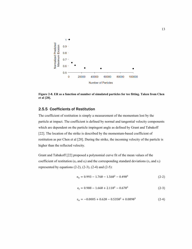
2.5.4 Number of Simulated Particle

The number of particle striking the surface influences the ER until the ER becomes

independent of it. Chen et al [20] showed that the predicted ER is independent of number

of simulated particle when the number is larger than 20,000 for an elbow fitting shown in

Figure 2-7 and for tee fitting as well as shown in Figure 2-8.

Figure 2-7. ER as a function of number of simulated particles for elbow fitting. Taken from

Chen et al [20].

13

Figure 2-8. ER as a function of number of simulated particles for tee fitting. Taken from Chen

et al [20].

2.5.5 Coefficients of Restitution

The coefficient of restitution is simply a measurement of the momentum lost by the

particle at impact. The coefficient is defined by normal and tangential velocity components

which are dependent on the particle impingent angle as defined by Grant and Tabakoff

[22]. The location of the strike is described by the momentum-based coefficient of

restitution as per Chen et al [20]. During the strike, the incoming velocity of the particle is

higher than the reflected velocity.

Grant and Tabakoff [22] proposed a polynomial curve fit of the mean values of the

coefficient of restitution (en and et) and the corresponding standard deviations (ɛn and ɛt)

represented by equations (2-2), (2-3), (2-4) and (2-5):

en = 0.993 − 1.76θ − 1.56θ2 − 0.49θ3 (2-2)

et = 0.988 − 1.66θ + 2.11θ2 − 0.67θ3 (2-3)

εn = −0.0005 + 0.62θ − 0.535θ2 + 0.089θ3 (2-4)

14

εt = 0 + 2.15θ − 5.02θ2 + 4.05θ3 − 1.085θ4 (2-5)

Forder et al [23] showed that the particle incoming angle has a significant effect on the

coefficient of restitution and proposed the following equations (2-6) and (2-7).

en = 0.988 − 078θ + 0.19θ2 − 0.024θ3 + 0.0027θ4 (2-6)

et = 1 − 0.78θ + 0.84θ2 − 0.21θ3 + 0.028θ4 − 0.022θ5 (2-7)

15

3 Computational Approaches

In the last decade, CFD modeling was dramatically increased for use in the prediction of

the wear damage in order to determine the system performance before adapting or after

executing the systems. Researchers conducted experiments to enhance the database for

CFD validation. By numerically solving the fluid flow equations and particle equations, the

CFD method creates a simulation model that represents behavior of flow in real

environment. For example, AEA Technology [24] developed CFX software, which was

one of the early CFD to predict erosion.

The procedure of CFD modeling essentially involves three main stages; 1) flow modeling,

2) particle modeling using Discrete Phase Model (DPM), and 3) erosion prediction

calculations. These three main stages in CFD modeling will be discussed in this chapter.

3.1 CFD Flow Modeling

The mass and momentum conservation are given by equations (3-1), (3-2) and (3-3) in

reference to Fluent [25], [26].

∂

∂t( αqρq) + ∇. ( αqρq vq ) = ∑ ( mpq − mqp)

np=1 (3-1)

∂

∂t( αqρq vq ) + ∇ ∙ (αqρqvq vq ) = −αq∇p + ∇ ∙ τq + αqρq g + ∑( R pq + mpqv pq − mqpv qp)

n

p=1

+

( F q + F lift,q + F wl,q + F vm,q + F td,q) (3-2)

��𝒒 = 𝛂𝐪𝛍𝐪(𝛁 �� 𝐪 + 𝛁 �� 𝑻𝐪) + 𝛂𝐪 (𝝀𝒒 −𝟐

𝟑 𝛍𝐪) 𝛁 ∙ �� 𝐪�� (3-3)

16

where (��𝑝𝑞) is the mass transfer from (p→ q), ( 𝛼𝑞) is the phase volume fraction, (𝜌𝑞) the

density of phase, (𝑣𝑞 ) is the velocity of phase (q), ��𝑞 is the phase stress-strain tensor

represented by (��𝑞 = 𝛼𝑞), µq is the shear viscosity of phase, 𝜆𝑞, F q is external body force,

F lift,q is the lift force, F wl,q is the wall lubrication force, F vm,q is the virtual mass force,

F td,q is the turbulent dispersion force, R pq is the interaction force between phases, p is the

pressure shared by all phases and v pqis the interphase velocity between the two phases.

3.1.1 Turbulence Modeling

A number of turbulence models are available in Fluent such as the Spalart-Allmaras model,

k- ɛ models, k-ω models, Reynolds stress model (RSM) and Large Eddy simulation model

(LES). In this study, we used RSM.

There is a trade-off between accuracy and computational cost for each of these models.

From Spalart-Allmaras to Large Eddy simulation models, the accuracy and computational

cost increase.

Fluent [25] comments on the choice of turbulence that; “The choice of turbulence model

will depend on considerations such as the physics encompassed in the flow, the established

practice for a specific class of problem, the level of accuracy required, the available

computational resources, and the amount of time available for the simulation”.

3.1.2 Near-Wall Treatment

The near-wall treatment for turbulence substantially influences the precision of numerical

solutions due to for example large gradient at wall.

For the precision of numerical solutions, the affordable Y+ value in general is (Y+ ≈ 30).

Fluent offers two approaches in order to resolve near wall region. The first approach is

called Wall Function Approach and the second called Near-Wall Model Approach. Fluent

[25] shows the difference between the two approaches in Figure 3-1. The mesh plays a

significant role to resolve the effect in Near-Wall Model Approach.

17

Fluent offers the following wall function approaches: Standard Wall Functions, the

Scalable Wall Functions, Non-Equilibrium Wall Functions and Enhanced Wall treatment.

In this study, we used the Scalable Wall Functions.

Figure 3-1. The two approaches for Near-Wall Treatments. Taken from Fluent [25].

Accuracy will increase moving from Standard Wall Functions to Enhanced Wall Treatment

as will the cost of computation.

3.2 Discrete Phase Modeling (DPM)

The particles that are carried with the fluid are simulated using Discrete Phase Modeling

(DPM) technique in Fluent as the second phase in order to simulate the particle trajectories

and interactions. DPM correctly handles particle movement in association with fluid using

Lagrangian tracking scheme.

The Lagrangian DPM model follows Euler-Lagrange approach as per Fluent Theory guide

[25] ” The fluid phase is treated as a continuum by solving the Navier-Stokes equations,

while the dispersed phase is solved by tracking a large number of particles, bubbles, or

18

droplets through the calculated flow field. The dispersed phase exchange momentum,

mass, and energy with the fluid phase”.

A number of factors related to the injection material properties, such as diameter, velocity,

and total flow rate, can limit the use of DPM when the volume fraction greatly exceeds 10–

12%. In that case, a Multiphase Models method is used instead of the DPM.

When there is an exchange of momentum or heat between the fluid and particle, Fluent

offers the ability to include or exclude those effects by using: Coupled or Uncoupled DPM.

If the particles influence the flow solution, then the Coupled DPM will used. If not,

uncoupled DPM is preferred. In this study, we used Coupled DPM.

3.2.1 Particle Turbulent Dispersion

Tracking particles in a turbulent flow requires consideration of turbulent dispersion of the

particles. Fluent offers two models to predict the dispersion: Stochastic Tracking and

Cloud Tracking. The Stochastic Tracking is based on mean flow velocity and instantaneous

fluctuation in the turbulent velocity. On the other hand, the Cloud Tracking is based

tracking the on the statistical evolution of cloud of particles about mean trajectory as per

Fluent [25]. In this study, we used Stochastic Tracking.

3.3 Erosion Prediction Formulae

In the last two decades, the Erosion/Corrosion Research Center (E/CRC) at the University

of Tulsa has contributed significantly to the area of erosion prediction in general and

developed an empirical form of ER ( Ahlert [27], Mclaury [28], [29], [30], [31] [31] [32] ).

There are several empirical erosion equations. For instance, Zhang [4] published an erosion

prediction equation for liquid flow with sand using Inconel 625 wall material. Oka [33],

[34] published an empirical erosion equation with air flow for three different wall

materials; Aluminum, Carbon Steel, and Stainless Steels. In addition, Oka used three types

of particles: Angular SiO2, SiC and Glass Beads.

19

Most of the empirical model for erosion prediction in the literature generally takes the

following form in equation (3-4).

ER = K f(∅)vpn (3-4)

Where (ER) is the erosion rate of the target material, K is the constant depending on the

target property, particle shape, particle hardness and is mainly obtained through

experiments. f(∅) is a dimensionless function of the impact angle, vp is the velocity of the

particle, and n is the material-dependent index.

This section discussed the way that Fluent considers the erosion formula and an erosion

empirical formula recently published by Vieira et al [2]. The formula by Vieira et al is

assumed for BP in Sales Gas in the current work.

3.3.1 Fluent Default Erosion Model

The ER in ANSYS Fluent [25] is given by the following equation (3-5)

ER = ∑Cd vp

n f(θ) m

Aface

N particlesp=1 (3-5)

Where �� is defined as the particle mass flow rate, Cd particle diameter function, A face

surface area of face, f(∅) is a dimensionless function of the impact angle and N Particles is the

number of particles.

Those values are incorporated in Fluent by using either Custom Field Function (CFF) or

User Defined Function (UDF). CFF was utilized to represent the value in the form of

constant, polynomial, piecewise polynomial or piecewise linear relation, while UDF uses C

programming language to incorporate the erosion equation. CFF is considered relatively

simple approach while UDF enhances the capability to control the variable in more

complicated forms. In this study, we use UDF.

20

3.3.2 Vieira Model

Vieira et al [2] is the latest published empirical erosion prediction formula by the

Erosion/Corrosion Research Center (E/CRC) at the University of Tulsa, Oklahoma. The

model was found specifically for flow of air with sand particles. The wall materials was

Stainless Steel 316 and the flow domain was an elbow-shaped pipe spool.

The Vieira et al formula’s are given by Equations (3-6) and (3-7).

𝐸𝑅 = 2.16 × 10−8 𝐹𝑠 × 𝑣𝑝2.41 × 𝑓(𝜃) (3-6)

𝑓(𝜃) = 0.65(𝑠𝑖𝑛𝜃)0.15(1 + 1.48(1 − 𝑠𝑖𝑛𝜃))0.85 (3-7)

Based on Scanning Electron Microscope (SEM) analysis for the sand particles utilized in

their research, the particle sharp factor for 300 and 150 μm equals 1 and 0.5, respectively.

In this study, we used Vieira et al formula where we assumed BP impact angle, particle

diameter function and the material-dependent index are similar to those of sand. The Shape

factor is assumed to be 1 for all particles.

21

4 Methodology

The methodology for the study will be discussed in this chapter.

4.1 Methodology

In order to study the internal damage of the plant piping system by BP, Fluent ANSYS was

selected as the primary simulation tool of the study. The study is based on real operation

conditions for one of the Sales Gas plant in Saudi Aramco and the cases studied use these

real operational conditions. It focuses on modeling erosion phenomena in a selected pipe

spool with a 90º degree elbow bend matching the configuration in the field. Fittings, such

as the bended elbow, can change the particle flow direction and may cause significant

erosion damage. These fittings can experience the highest ER. The effects of variation in

stream velocity, pressure drops, in addition to the change in particle size are examined.

Validation studies were conducted by comparing to previous result.

4.1.1 Simulation Configuration

Numerical set up will be introduce in the following sections.

4.1.1.1 Flow Domain Geometry

The selected pipe spool considered in the study is as follows: The geometries consist of a

straight inlet followed by a 90º elbow with curvature radius of r/D=1.5. The pipe outside

diameter (OD) is 30 inches with an inlet and outlet length of 45 inches as shown in

Figure 4-1 and Figure 4-2.

22

Figure 4-1. Configuration of the modeling geometries.

Figure 4-2. The numerical configuration in Fluent.

4.1.2 Grid Convergence Study

Structured grid with hexahedral shape mesh was selected. In order to capture the velocity

gradients near the wall, in the vicinity of the pipe wall the grid was greatly refined by

adding more grid points there. This process helps to increase the resolution in the vicinity

23

of the wall and also lowers the Y+ value. Two more important quality measurements for the

grid are skewness and orthogonal quality. Skewness determines how much the generated

mesh cell and elements differ from an ideal mesh cell or element. Skewness is scaled from

0 to 1, where the closer the value is to 0, the better quality is has the cell. On the other

hand, the Orthogonal Quality (OQ) of a cell closer to 1 indicates better cell quality. Both

Figure 4-3, Figure 4-4 and Figure 4-5 show the mesh utilized in the grid independence

study where the mesh is greatly refined in the vicinity of the pipe wall.

Figure 4-3. Mesh utilized in the study.

24

Figure 4-4. Mesh for the inlet face.

Figure 4-5. Mesh at the vicinity of wall.

4.1.3 Boundary Conditions

Pressure at the inlet and the outlet are specified as the boundary conditions. The pressure

differences are chosen such that the velocity of the gas represents those observed in the

operational condition in the plant. Four pressure differences between ∆𝑃 the inlet and

outlet pipe are considered 0.25, 0.5, 1 and 1.25 psi. The turbulent intensity selected is 5%,

25

and the turbulent viscous ratio (the ratio between the turbulent viscosity and the molecular

viscosity) is 10 as recommended by Fluent [25]for internal flow.

4.1.4 Solver Setting

The flow was assume to be steady state flow. The turbulent viscosity model is the

Reynolds Stress Model (RSM) with linear pressure strain and scalable wall functions for

the near wall treatment. To account for the interaction between the particles and turbulent

eddies, the Discrete Phase Model (DPM) with 10 Continuous Phase Iterations per DPM.

The maximum value of sharp factor of 1 is considered. The maximum number of step

tracking is 500,000. The mass flow rate of particle injection is 0.0024 kg/sec injected

normal into the inlet face with speed matching the flow speed at the field condition.

The particle turbulent dispersion is stochastic tracking with a discrete random walk model

and a random eddy lifetime to consider the interaction between particles and turbulent

eddies. The number of particles tracked in this study was 22,358. To substantiate the study

findings, the erosion model was activated to calculate the ER. The Sales Gas fluid is an

isothermal gas with a density ρ of 21.02 kg/m3 and a viscosity μ of 1.33e–05 Pa·s based on

a sample from the field. The pipe material used was carbon steel with a density of 7850

kg/m3, and the BP density is 5150 kg/m3 (El-Saadawy and Sherik [1]). The solution

methods based on pressure-velocity coupling is used. The residual tolerance was set to 10-

4. The pressure interpolation scheme was set as standard, the momentum scheme was

second-order upwind, and turbulent kinetic energy and the turbulent dissipation rate were

calculated with first order upwind.

The latest empirical erosion prediction formula by Vieira et al [2] was utilized as the UDF

in the calculation of ER.

26

5 Results and Discussion

In this chapter, the two validation models will be discussed and we will present the result

of the grid resolution study. In addition, the behavior of ER as we change the particle size,

number, Sales Gas velocity, and pressure drops will discussed. We will also examine the

effect of Stokes and Reynold numbers.

5.1 Validation Modeling

Verification and validation were conducted by reproducing previous result by Vieira et al

[2] and Njobuenwu and Fairweather [3].

Figure 5-1 shows the comparison of the contours of ER between the Vieira et al model and

the current model. A similar erosion prediction with V-shaped pattern seen in Vieira was

reproduced here with slight difference in the magnitude of erosion. The air fluid is an

isothermal with a density ρ of 1.2 kg/m3 and a viscosity μ of 1.8e–05 (kg/m-s). The pipe

material used was Stainless steel 316 with a density of 7990 kg/m3, and the sand density is

2650 kg/m3.

Figure 5-1. Comparison of ER between Vieira et al model (left) and the current model (right).

27

Figure 5-2 shows the maximum primary and secondary wear location in a pipe bend

studied in Njobuenwu and Fairweather [3] model. A similar normalized erosion pattern

with primary and secondary wear location seen in Njobuenwu and Fairweather [3] was

reproduced here with slight difference in the location of maximum secondary wear.

Figure 5-2. The primary and secondary wear location in pipe bend similar to Njobuenwu and

Fairweather [3].

5.2 Grid Resolution Study

Four different mesh sizes were chosen with an approximate factor of two difference in the

total number of node and element between each of them, and with a Y+ factor of a half

difference between each mesh. The number of particles used was nearly 22,358 and the

velocity of fluid and particles is17.6 m/s. The pipe diameter is 0.762 m (30 inches) and the

particle diameter is 3 µm. The boundary condition setting represent the current operation

condition for Sales Gas piping associated with debris of BP. Table 5-1 shows the result of

the grid resolution study for the case of ΔP = 0.25 psi.

0

0.2

0.4

0.6

0.8

1

1.2

0 20 40 60 80 100

No

rmal

ised

Ero

sio

n (

E/E

max

)

Bend Angle (degree)

Secondary

Primary

28

Table 5-1. Grid resolution study. 𝚫𝐏 = 0.25 psi.

No Mesh size Mesh quality ER

No. of

Node

No. of

Element

Skewness quality Orthogonal quality Y+ AWA

(mm/year)

Max Min. Avg. Max Min. Avg.

1 232,704 227,430 0.505 2.17e-2 5.49e-2 0.999 0.796 0.994 80.7 0.014

2 501,676 492,756 0.633 1.45e-2 4.64e-2 0.999 0.588 0.995 41.8 0.013

3 958,566 943,888 0.599 1.06e-2 4.49e-2 0.999 0.661 0.994 22.9 0.012

4 4,668,768 4,618,768 0.616 3.16e-3 3.71e-2 0.999 0.617 0.996 11.5 0.011

From the study, we found convergence is approximately first order. So, for this study, a

mesh size of 377,190 nodes and 370,504 elements are chosen with a Y+ equal to 30. The

mesh average skewness is 4.7524e-02, and the average orthogonal quality is 0.9951.

Noted that, the simulated ER is fairly close to the measured ER from the field and the

difference is about 28%. Also note here, the simulation target a specific operation

condition with ER measure from field.

5.2.1 Effect of Number of Simulated Particles

Chen et al [20] showed that the predicted ER is independent of the number of simulated

particles when the number is larger than 20,000 for an air flow with sand particles. In the

current work, a similar pattern is observed for the Sales Gas with the BP particles. Thus,

Figure 5-3 shows the independence of ER on the number of particle when the number is

larger than 20,000.

29

Figure 5-3. ER as a function of particles the number of simulated particles.

5.3 Parametric Study

Parametric studies will be presented in this section. The effect of particle size, Sales Gas

velocity, and pressure drops will be examined. The effect of Stokes and Reynolds numbers

will also be discussed.

5.3.1 Particle Size

Figure 5-4 shows that the ER increases with the BP particle size. A steep rise was noticed

as the particle size is increased from 0.1 to 3 µm, followed by a slight decrease and then

increase as particle size changed from 3 µm to 300 µm for the cases of ΔP of more than

0.25 psi. The highest increase of the ER is nearly 14%, 11%,8%,8% for the cases of

(0.25,0.5,1.0 and 1.25) respectively with a factor of 2 increase in the particle size. The case

of 0.25 psi is representative of the normal operational conditions of the system, and the

0.0124

0.0124

0.0125

0.0125

0.0126

0.0126

2,000 22,000 42,000 62,000 82,000 102,000

Ero

sio

n R

ate

(mm

/yea

r)

Number of Simulated Particles

30

maximum simulated ER, is 0.029 mm/year for particles of size of 300 µm. If there is

deposition on the line due to either accumulations of BP or other reasons, the cases 0.5, 1

and 1.25 pressure drops can occurred.

Figure 5-4. ER as a function of BP particle size and different ΔP.

Oil and gas industry set an acceptable erosion allowance once debris was anticipated to be

transported with the fluid. American Petroleum Institute (API) and other societies offer

guidelines for erosion limit to be considered by pipe designers. The pipe designer shall

predict the erosion behavior and determine the minimum required pipe thickness. Erosion

limit such as 1.6 mm, 3.0 mm or 6 mm are usually considered. In the Sales Gas piping, the

designer chooses 1.6 mm, which is sufficient based on our finding for the 30-year life cycle

of a pipe for the majority of 0.25 and 0.5 psi cases. Table 5-2 summarizes the ER for

different particle sizes for ΔP =0.25 and 0.5 psi cases.

0.00

0.02

0.04

0.06

0.08

0.10

0.12

0.14

0.16

0.18

0.20

1.00E-08 5.00E-05 1.00E-04 1.50E-04 2.00E-04 2.50E-04 3.00E-04

Ero

sion R

ate

(mm

/yea

r)

Particles Size ( m)

1.25 psi

1 psi

0.5 psi

0.25 psi

31

Table 5-2. ER for different BP particle sizes for 𝚫𝐏 = 0.25 and 0.5 psi cases.

Particle Size (m) ER in (mm/year)

0.25 0.5

3.00E-04 0.0293 0.0646

1.50E-04 0.0243 0.0522

9.00E-05 0.0220 0.0457

7.50E-05 0.0213 0.0439

3.75E-05 0.0182 0.0386

2.00E-05 0.0147 0.0330

1.88E-05 0.0144 0.0326

1.00E-05 0.0143 0.0329

9.38E-06 0.0142 0.0329

4.69E-06 0.0136 0.0338

3.00E-06 0.0132 0.0344

2.34E-06 0.0121 0.0324

1.00E-06 0.0060 0.0177

1.00E-07 0.0045 0.0111

Table 5-3 presents the ER for different BP particle sizes for 1 and 1.25 psi cases. It is seen

that for 3 µm particles, the life cycle of the erosion allowance of the pipeline is reduced to

20 & 14 years for the case of 1 and 1.25 psi, respectively. Also, Increasing the pressure

drop by a factor of two can increase the ER by an average factor of 2.32.

32

Table 5-3. ER for different BP particles sizes for 𝚫𝐏 = 1 and 1.25 psi cases.

Particle Size (m) ER in (mm/year)

1 1.25

3.00E-04 0.1465 0.1909

1.50E-04 0.1171 0.1520

9.00E-05 0.1018 0.1322

7.50E-05 0.0972 0.1262

3.75E-05 0.0867 0.1134

2.00E-05 0.0780 0.1028

1.88E-05 0.0771 0.1026

1.00E-05 0.0771 0.1017

9.38E-06 0.0780 0.1032

4.69E-06 0.0861 0.1138

3.00E-06 0.0880 0.1159

2.34E-06 0.0864 0.1161

1.00E-06 0.0526 0.0736

1.00E-07 0.0273 0.0359

To examine the effect of particle density, simulation were performed with different particle

density. A similar trend was observed for the relation between ER and particle size for

different pressure drops for sand particles with a density of 7990 kg/m3 as shown in

Figure 5-5.

33

Figure 5-5. ER as a function of sand particle size.

5.3.2 Empirical Relation for Erosion Rate

Based on the simulation data, a simple empirical relation for ER can be delivered as given

in equation (5-1).

ER = 0.4377 × 𝑑𝑝 0.1508 × ΔP 1.211 (5-1)

where ER is the Erosion Rate in (mm / year), 𝑑𝑝 is the particle diameter in (m) and ΔP is

the pressure drop in psi. The empirical correlation explains 99.24% of the total variation in

the data and the regression coefficients are obtained by nonlinear least squares regression

using Matlab [35]. Figure 5-6 shows the relation between the ER and the particle size and

pressure drops in 3D surface plot along with the simulation data.

0

0.02

0.04

0.06

0.08

0.1

0.12

0.14

0.16

1.00E-08 1.00E-04 2.00E-04 3.00E-04

Ero

sio

n R

ate

(mm

/yea

r)

Particles Size

1 psi

0.5 psi

34

Figure 5-6. 3-D Surface plot for the ER versus particles size and pressure drop.

5.3.3 Effect of Particles Size on the Location of Maximum Erosion

The locations of maximum destruction in the elbow vary with particle size. Since particle

of larger sizes tend to move more independently from the air flow, they collide with fitting

such as elbow or tee strongly. Figure 5-7, Figure 5-8, Figure 5-9 and Figure 5-10 show the

location of area with maximum destruction for 300, 150, 90 and 75 µm particle. It can be

seen, when Stokes number is large, particle gain some independence from the flow stream

and strike the elbow as flow changes direction as per Friedlander and Johnstone [17].

35

Figure 5-7. The destruction of erosion for 300 µm BP particles. ER is in (kg/m2-s).


36



37

Unlike for larger particle. When particles are of smaller sizes such as 20 and 10 µm, the

flow stream and the area of maximum ER is at the outlet of the pipe spool. It clearly that

particle rebounds at the elbow and causes damage at different location. Figure 5-11,

Figure 5-12, Figure 5-13 and Figure 5-14 show that the maximum area of ER is at the

outlet of the pipe spool. Thus, at lower Stokes number, the particle starts to follow the flow

streamlines.

Figure 5-11. The destruction of erosion for 20 µm BP particles (1). ER is in (kg/m2-s).

38



39


For even smaller particles and lower Stokes number, erosion tend to be more dispersed, as

shown in Figure 5-15, Figure 5-16, Figure 5-17 and Figure 5-18. The magnitude of the ER

is however relatively small for low-pressure drops.

40

:



41


Figure 5-18. The destruction of erosion for 0.1 µm BP particles. ER is in (kg/m2-s).

42

5.3.4 Reynolds Number

Reynolds number is widely used to classify the flow type. As particle size increases, the

ER increases too. In DPM, Reynolds number is defined as per equation (5-2)

Re =ρ dp|up−u|

μ (5-2)

where u is the fluid phase velocity, up is the particle velocity, µ is the molecular viscosity

of the fluid, ρ is the density of fluid and dpis the particle diameter.

5.3.5 Fluid Velocity

To provide guideline for the plant operator to avoid high erosion rate and avoiding the

reduction of the life cycle of the system, the data are also plotted in terms of ER as a

function of the velocity of Sales Gas as shown in Figure 5-19. At low SG velocity, the ER

for most of the particle size is lower than the designed ER for the system. Where at high

velocity, the ER is higher than the designed ER. Noted that, the particle sizes of 3 µm and

smaller have magnitude of ER similar to 37 µm. Because particles smaller than 3 µm is

allowed to convey with SG. So, should pay attention to this result.

43

Figure 5-19. Relation between the ER and the Sales Gas velocity.

5.4 Future Work

A couple of experimental studies can be conducted for the calibration of the parameters of

erosion model in equations (3-6) and (3-7) and particle shape factor. As a result, a unique

ER equation specifically for the flow of Sales Gas with BP can be obtained. In addition,

the effects of erosion by BP particle can be studied further in different sections of pipeline

network, starting from the gas compressor that pushes the flow through the pipeline to the

cyclone separator vessels, filtration vessels, valves, different pipe fittings and fuel burners.

Not only can the ER be identified, but also the area of maximum destruction, required

erosion limit, and the life cycle of critical equipment can be predicted.

0

0.02

0.04

0.06

0.08

0.1

0.12

0.14

0.16

0.18

0.2

15 20 25 30 35 40 45

Ero

sio

n R

ate

(mm

/yea

r)

Velocity (m/s)

300 µm

150 µm

90 µm

75 µm

37 µm

20 µm

18 µm

10 µm

9.4 µm

4.7 µm

3 µm

2.3 µm

1 µm

0.1 µm

designed ER

for the system

44

Conclusion

In this study, the impact of BP particle size on the ER in Sales Gas piping system is

examined. The study helps the design engineer, maintenance personal, inspector and

operational personnel to predict the ER and the area of maximum destruction at normal and

disrupt operation condition. It also offers a handy empirical formulae to be utilized by plant

engineers and inspector to predict the ER based on the particle sizes and pressure drops.

Indeed, ER increases with the increase of the pressure drops, BP particles size and the

Sales Gas velocity. Thus, operating the Sales Gas system at lower possible velocity and

minimize the pressure drop in the pipe helps to lower the ER.

45

References

[1] E. Elsaadawy and A. Sherik, "Pipe diameter does not affect black powder

distribution, erosion," Oil Gas J, vol. 110, pp. 104-110, July, 2012.

[2] R. Vieira, A. Mansouri, B. McLaury and S. Shirazi, "Experimental and

computational study of erosion in elbows due to sand particles in air flow," Powder

Technology,, vol. 288, p. 339–353, January, 2016.

[3] D. Njobuenwu and M. Fairweather, "Modelling of pipe bend erosion by dilute

particle suspensions," Computers and Chemical Engineering, vol. 42, pp. 235-247,

2012.

[4] Y. Zhang, E. Reuterfors, B. McLaury, S. Shirazi and E. Rybicki, "Comparison of

computed and measured particle velocities and erosion in water and air flows," Wear,

vol. 263, p. 330–338, September, 2007.

[5] A. M. Sherik, "Black Powder-1: Study examines sources, makeup in dry gas

systems," Oil and Gas Journal, vol. 106, p. 54–59, August 2008.

[6] A. M. Sherik, "Black powder in sales gas transmission pipelines," Saudi Aramco,

vol. Fall, pp. 2-10, 2007.

[7] S. Khan and M. Al-Shehhi, "Review of black powder in gas pipelines - an industrial

perspective," J. Nat. Gas Sci. Eng 25, vol. 25, pp. 66-76, 2015.

[8] A. Sherik and E. El-Saadawy, "Erosion of control valves in gas transmission lines,"

Mater. Perform., vol. 52, no. 5, pp. 70-73, May 2013.

[9] A. Filali, L. Khezzar, M. Alshehhi and N. Kharoua, "A One-D approach for

modeling transport and deposition of Black Powder particles in gas network,"

Journal of Natural Gas Science and Engineering, vol. 28, pp. 241-253, January,

2016.

46

[10] I. Finnie, "Erosion of surfaces by solid particles," Wear, vol. 3, no. 2, pp. 87-103,

1960.

[11] I. Finnie, "Some reflections on the past and future of erosion," Wear, vol. 186–187,

pp. 1-10, July 1995.

[12] G. Sheldon and I. Finnie, "On the ductile behavior of nominally brittle materials

during erosive cutting," Trans. ASME, vol. 888, pp. 387-392, 1966.

[13] J. Ritter, Erosion of Ceramic Materials, Zurich, Switzerland: Trans. Tech

Publications, 1992.

[14] C. Smeltzer, M. Gulden and W. Compton, "Mechanisms of the erosion of metals by

solid particles," Journal of Basic Engineering, vol. 19, pp. 639-654, September 1970.

[15] M. Jones and R. Lewis, "Solid Particle Erosion of a Selection of Alloy Steels," in

Proceedings of the 5th International Conference on Erosion by Liquid and Solid

Impact, September, 1979.

[16] ANSYS, "Multiphase Modeling using ANSYS Fluent," ANSYS, December 15,

2015..

[17] S. Friedlander and H. Johnstone, "Deposition of suspended particles from turbulent

gas streams.," Industrial Eng. Chem, vol. 49, pp. 1151-1156, 1957.

[18] V. Nguyen, Q. Nguyen, C. Lim, Y. Zhang and B. Khoo, "Effect of air-borne

particle–particle interaction on materials erosion," Wear, Vols. 322-323, pp. 17-31,

2015.

[19] C. Duan and V. Karelin, Abrasive Erosion and Corrosion of Hydraulic Machinery.,

vol. 2, London: Imperial College Press, 2002.

[20] X. Chen, B. McLaury and S. Shirazi, "Application and experimental validation of a

computational fluid dynamics CFD based erosion prediction model in elbows and

plugged tees," Computer & Fluids, vol. 33, p. 1251–1272, December, 2004.

[21] R. Badruddin and S. Bahadur, "Erodent particle characterization and the effect of

particle size and shape on erosion," Wear, vol. 138, p. 189–208, June 1990.

47

[22] G. Grant and W. Tabakoff, "Erosion Prediction in Turbomachinery Resulting from

Environmental Solid Particles," Journal of Aircraft,, vol. 12, pp. 471-478, 1975.

[23] A. Forder, M. Thew and D. Harrison, "Numerical investigation of solid particle

erosion experienced within oilfield control valves," Wear, vol. 216, pp. 184-193,

April, 1998.

[24] A. Technology, CFX 4.2 Flow Solver, Oxfordshire, U.K: AEA Technology Inc,

1997.

[25] ANSYS, ANSYS Theory guide, Release 17.0, ANSYS, Inc, 2016.

[26] ANSYS, ANSYS User Manual, Release 17.0, ANSYS, Inc, 2016.

[27] K. Ahlert, "Effects of particle impingement angle and surface wetting on solid

particle erosion of AISI 1018 steel," Department of Mechanical Engineering, The

University of Tulsa, 1994.

[28] B. S. McLaury, Predicting solid particle erosion resulting from turbulent fluctuations

in oilfield geometries, Tulsa: The University of Tulsa, 1996.

[29] B. S. McLaury and S. A. Shirazi, "An alternate method to API RP 14E for predicting

solids erosion in multiphase flow," Journal of Energy Resources Technology, vol.

122, p. 115–122, May, 2000.

[30] J. K. Edwards, B. S. McLaury and S. Shirazi, "Supplementing a CFD code with

erosion prediction capabilities," in ASME Fluids Engineering Division Summer

Conference, Washington DC, June 21–25, 1998.

[31] J. K. Edwards, B. S. McLaury and S. A. Shirazi, "Modeling solid particle erosion in

elbows and plugged tees," Journal of Energy Resources Technology,, vol. 123, p.

277–284, June, 2001.

[32] B. S. McLaury, A model to predict solid particle erosion in oil field geometries,

Tulsa: The University of Tulsa, 1993.

[33] Y. Oka, K. Okamura and T. Yoshida, "Practical estimation of erosion damage caused

by solid particle impact Part 1," Wear, vol. 259, pp. 95-101, July –August, 2005.

48

[34] Y. Oka and T. Yoshida, "Practical estimation of erosion damage caused by solid

particle impact Part 2," Wear, vol. 259, pp. 102-109, July –August, 2005.

[35] T. MathWork, MATLAB 2016 R, Natick, Massachusetts, United States: The

MathWorks, Inc, 2016.

Numerical Study of Erosion of the Internal Wall of Sales ...

Documents

Transcript of Numerical Study of Erosion of the Internal Wall of Sales ...