Numerical studies of transition in wall-bounded ﬂows Ori...

Numerical studies of transition in wall-bounded flows

by

Ori Levin

December 2005Technical Reports from

KTH MechanicsSE-100 44 Stockholm, Sweden

Typsatt i AMS-LATEX.

Akademisk avhandling som med tillstand av Kungliga Tekniska Hogskolan iStockholm framlagges till offentlig granskning for avlaggande av teknologiedoktorsexamen fredagen den 16:e december 2005 kl 10.15 i sal F3, F-huset,Kungliga Tekniska Hogskolan, Lindstedsvagen 26, Stockholm.

c©Ori Levin 2005

Universitetsservice US-AB, Stockholm 2005

Numerical studies of transition in wall-bounded flows

Ori Levin 2005

KTH MechanicsSE-100 44 Stockholm, Sweden

Abstract

Disturbances introduced in wall-bounded flows can grow and lead to transitionfrom laminar to turbulent flow. In order to reduce losses or enhance mixingin energy systems, a fundamental understanding of the flow stability and tran-sition mechanism is important. In the present thesis, the stability, transitionmechanism and early turbulent evolution of wall-bounded flows are studied.The stability is investigated by means of linear stability equations and thetransition mechanism and turbulence are studied using direct numerical sim-ulations. Three base flows are considered, the Falkner–Skan boundary layer,boundary layers subjected to wall suction and the Blasius wall jet. The stabil-ity with respect to the exponential growth of waves and the algebraic growthof optimal streaks is studied for the Falkner–Skan boundary layer. For thealgebraic growth, the optimal initial location, where the optimal disturbance isintroduced in the boundary layer, is found to move downstream with decreasedpressure gradient. A unified transition prediction method incorporating the in-fluences of pressure gradient and free-stream turbulence is suggested. Thealgebraic growth of streaks in boundary layers subjected to wall suction is cal-culated. It is found that the spatial analysis gives larger optimal growth thantemporal theory. Furthermore, it is found that the optimal growth is largerif the suction begins a distance downstream of the leading edge. Thresholdsfor transition of periodic and localized disturbances as well as the spreading ofturbulent spots in the asymptotic suction boundary layer are investigated forReynolds number Re = 500, 800 and 1200 based on the displacement thicknessand the free-stream velocity. It is found that the threshold amplitude scaleslike Re−1.05 for transition initiated by streamwise vortices and random noise,like Re−1.3 for oblique transition and like Re−1.5 for the localized disturbance.The turbulent spot is found to take a bullet-shaped form that becomes moredistinct and increases its spreading rate for higher Reynolds number. TheBlasius wall jet is matched to the measured flow in an experimental wall-jetfacility. Both the linear and nonlinear regime of introduced waves and streaksare investigated and compared to measurements. It is demonstrated that thestreaks play an important role in the breakdown process where they suppresspairing and enhance breakdown to turbulence. Furthermore, statistics fromthe early turbulent regime are analyzed and reveal a reasonable self-similarbehavior, which is most pronounced with inner scaling in the near-wall region.

Descriptors: Boundary layer, suction, wall jet, streaks, waves, periodic dis-turbance, localized disturbance, turbulent spot, algebraic growth, exponentialgrowth, stability, transition thresholds, transition prediction, PSE, DNS.

Preface

This thesis considers the disturbance growth, transition and turbulent evolu-tion of wall-bounded flows. The thesis is divided in two parts, the first part isa short introduction to the field and a summary of the following papers. Thepapers are re-set in the present thesis format and included in the second partof the thesis.

Paper 1. Levin, 0. & Henningson, D. S. 2003 Exponential vs algebraicgrowth and transition prediction in boundary layer flow. Flow, Turbulence and

Combustion 70, 183–210.

Paper 2. Bystrom, M. G., Levin, 0. & Henningson, D. S. 2005 Optimaldisturbances in suction boundary layers. Submitted in a revised version.

Paper 3. Levin, 0., Chernoray, V. G., Lofdahl, L. & Henningson,

D. S. 2005 A study of the Blasius wall jet. Journal of Fluid Mechanics 539,313–347.

Paper 4. Levin, 0., Davidsson, E. N. & Henningson, D. S. 2005 Tran-sition thresholds in the asymptotic suction boundary layer. Physics of Fluids,In press.

Paper 5. Levin, 0. 2005 Turbulent spots in the asymptotic suction boundarylayer.

Paper 6. Levin, 0., Herbst, A. H. & Henningson, D. S. 2005 Earlyturbulent evolution of the Blasius wall jet. Submitted.

iv

PREFACE v

Division of work between authors

The first paper deals with the energy growth of eigenmodes and non-modaloptimal disturbances in the Falkner–Skan boundary layer with favorable, zeroand adverse pressure gradients. The numerical codes are based on alreadyexisting codes at KTH Mechanics. The numerical implementations needed forthis work were performed by Ori Levin (OL). The development of the theoryas well as the writing of the manuscript itself were both carried out by OL withsome assistance from Dan Henningson (DH).

The second paper is devoted to the energy growth of non-modal optimaldisturbances in boundary layers subjected to wall suction. The numerical codefor the spatial analysis is the same as for paper 1 with new subroutines forthe base flow. The work was performed by Martin Bystom (MB) as part ofhis Master Thesis with OL as the advisor. The writing was done by MB withsome assistance from OL and DH.

The third paper is a numerical and experimental study of the stability ofthe Blasius wall jet. The work is a cooperation between KTH Mechanics andThermo and Fluid Dynamics at Chalmers University of Technology (TFD).The numerical codes for the linear analysis are the same as for paper 1 withnew subroutines for the base flow. The Direct Numerical Simulations were per-formed with a numerical code, already in use for many research projects. Thecode is based on a pseudospectral technique and is developed originally by An-ders Lundbladh and DH. The numerical implementations needed for this workwere performed by OL. The experimental work was done by Valery Chernoray(VC) at TFD. The writing was carried out by OL with some assistance fromVC, Lennart Lofdahl at TFD and DH.

The fourth paper deals with energy thresholds for transition in the asymp-totic suction boundary layer disturbed by streamwise vortices, oblique wavesand noise. The numerical code for the temporal simulations is the same as forpaper 3 with minor implementations by OL in order to account for the massflux through the wall. The work was performed by OL and Niklas Davidsson(ND) and the writing was done by OL and ND with some advise from DH.

The fifth paper is on the thresholds for transition of localized disturban-ces, their breakdown to turbulence and the development of turbulent spots inthe asymptotic suction boundary layer. The numerical code for the temporalsimulations is the same as for paper 4. All the work was carried out by OLwith some advise from DH.

The sixth paper is devoted to the early turbulent evolution of the Blasiuswall jet. The numerical code for the spatial simulation, carried out by OL, isthe same as for paper 3. All the figures and animations were prepared by OL.The analysis of the statistics was performed by OL and Astrid Herbst (AH).The writing was done by OL and AH with some advise from DH.

Contents

Abstract iii

Preface iv

Part 1. Summary 1

Chapter 1. Introduction 3

Chapter 2. Weak disturbances 7

2.1. Waves 7

2.2. Streaks 8

2.3. Growth of weak disturbances 9

2.3.1. Linear disturbance equations 10

2.3.2. Algebraic growth 11

2.3.3. Exponential growth 12

2.4. Application to the Falkner–Skan boundary layer 12

2.4.1. Comparison of algebraic and exponential growth 12

2.4.2. Transition prediction based on linear theory 14

2.5. Application to boundary layers with wall suction 17

2.5.1. Suction boundary layers 17

2.5.2. Algebraic growth 18

2.6. Application to the Blasius wall jet 21

2.6.1. Comparison of linear theory with experiments 21

Chapter 3. Strong disturbances 23

3.1. Numerical method and disturbance generation 23

3.2. DNS of the Blasius wall jet 24

3.2.1. Spectral analysis 24

3.2.2. Flow structures 25

3.2.3. Subharmonic waves and pairing 28

3.3. DNS of the asymptotic suction boundary layer 28

vii

viii CONTENTS

3.3.1. Energy thresholds for periodic disturbances 28

3.3.2. Amplitude thresholds for localized disturbances 32

Chapter 4. Turbulence 35

4.1. The essence of turbulence 35

4.2. Spots in the asymptotic suction boundary layer 36

4.3. Turbulence statistics of the Blasius wall jet 39

Chapter 5. Conclusions 42

Acknowledgment 44

Bibliography 45

Part 2. Papers 49

Paper 1. Exponential vs algebraic growth and transition

prediction in boundary layer flow 53

Paper 2. Optimal disturbances in suction boundary layers 83

Paper 3. A study of the Blasius wall jet 105

Paper 4. Transition thresholds in the asymptotic suction

boundary layer 151

Paper 5. Turbulent spots in the asymptotic suction

boundary layer 177

Paper 6. Early turbulent evolution of the Blasius wall jet 201

Part 1

Summary

CHAPTER 1

Introduction

A solid material possesses the property of rigidity, implying that it can with-stand moderate shear stress without a permanent deformation. A true fluid,on the other hand, is by definition a material with no rigidity at all. Subjectedto shear stress, no matter how small this stress may be, a fluid is bound tocontinuously deform. The fluids that all of us are most familiar with are wa-ter and air. Water is a liquid, while air is a gas, but that distinction is lessimportant than might be imagined when it comes to fluid dynamics.

A fluid flow is usually defined as either laminar or turbulent. The laminarflow is characterized by an ordered, layered and predictable motion while theturbulent state consists of a chaotic, swirly and fluctuating motion. The differ-ence between the two kinds of motions can easily be visualized in the kitchenwhile pouring water from the tap. If the tap is opened only a bit, the waterthat flows from the faucet is smooth and glassy, because the flow is laminar.When the tap is opened further, the flow speed increases and the water all ofa sudden becomes white with small bubbles, accompanied by a louder noise.The jet of water has then become irregular and turbulent and air is mixed intoit. The same phenomenon can be seen in the smoke streaming upward intostill air from a burning cigarette. Immediately above the cigarette, the flowis laminar. A little higher up, it becomes rippled and diffusive as it becomesturbulent.

The two above everyday examples illustrate the effect of flow speed anddistance on the cause of turbulence. As the flow velocity or the characteristiclength of the flow problem increases, small disturbances introduced in the flowamplify and the laminar flow break down to turbulence. This phenomenon iscalled transition. There is one more quantity affecting the state of the flow,namely the viscosity of the fluid. For sufficiently large viscosity, motions thatwould cause turbulence are damped out and the flow stays laminar. For exam-ple, it is very hard to get the flow from a bottle of sirup to become turbulentsince the viscosity of sirup is very high. Air with its considerably lower viscositybecomes turbulent very easily.

The basic difference between laminar and turbulent flows was dramaticallydemonstrated by Osborne Reynolds in a classical experiment at the hydraulicslaboratory of the Engineering Department at Manchester University. Reynolds(1883) studied the flow inside a glass tube by injecting ink at the centerline ofthe pipe inlet. At low flow rates, the flow stayed laminar and the dye stream

3

4 1. INTRODUCTION

was observed to follow a well-defined straight path inside the tube. As theflow rate was increased, at some point in the tube, the dye streak broke upinto a turbulent motion and spread throughout the cross section of the tube.He found that the value of a dimensionless parameter, now called Reynoldsnumber, Re = Ud/ν, where U is the mean velocity of the water through thetube, d the diameter of the tube and ν the kinematic viscosity of the water,governs the transition from laminar to turbulent flow. Reynolds made it clear,however, that there is no single critical value of Re, above which the flowbecomes unstable and transition may occur. The whole matter is much morecomplicated and very sensitive to disturbances from the surroundings enteringthe pipe inlet. In fact, transition and its triggering mechanisms are even todaynot fully understood.

In a laminar flow, the shear stresses are smaller than in a turbulent flowand as a consequence, the friction drag over the surface of a wing is much lower.On the other hand, a laminar flow can not stay attached to the upper surfaceof a wing as far downstream as a turbulent flow since the pressure increasesdownstream. Instead, laminar separation occurs resulting in the formation ofa wake and increased pressure drag. However, for a turbulent flow, separationis delayed due to the mixing provided of the chaotic motion and the total dragforce decreases. That is also the reason why golf balls have dimples over thesurface, to enforce turbulence and a smaller wake behind it. Due to the excellentmixing of a turbulent flow, it is required in chemical reactors and combustionengines. In some applications, it is important to keep the flow laminar andin others to enforce turbulence. Therefore an increased understanding of thetriggering mechanisms of transition from laminar to turbulent flow and itsforegoing amplification of introduced disturbances is important.

For transition to take place, some part of the flow has to be unstable to in-troduced disturbances. Such flows usually possess some kind of velocity shear,like the boundary layer and the free shear layer shown in figure 1.1. The bound-ary layer is the flow, in the lower part of the figure, over the horizontal flat platesubjected to a uniform oncoming flow with velocity U0. Due to viscosity, theflow velocity varies from zero at the wall to the free-stream velocity a distanceof the boundary layer thickness above the wall. The free shear layer, in theupper part of the figure, evolves from the difference in the streamwise velocitybelow the vertical wall and behind it. The streamwise velocity varies from themaximum velocity U0 below the shear flow to zero above it. The thickness ofthe shear layers grow as the flow develops downstream. The combined flow fieldin figure 1.1 and the downstream interaction of the shear layers are defined asthe Blasius wall jet.

The whole transition process consists of three stages: receptivity, distur-bance growth and breakdown. In the receptivity stage, disturbances are initi-ated in the part of the flow where velocity shear is present. Typical sources fromwhich disturbances can enter the shear flow are free-stream vortical structures,free-stream turbulence, acoustic waves, and for the case of wall-bounded shear

1. INTRODUCTION 5

x

y

U0

Figure 1.1. Wall-bounded and free shear layer flow that to-gether form a wall jet.

flows, surface roughness and vibrations. Once a disturbance is introduced inthe shear flow, it may grow or decay according to the stability characteristics ofthe base flow (the undisturbed flow field). When the disturbances are yet weakcompared to the base flow, one can study linearized stability equations to de-termine the disturbance growth. In fact, the linear mechanisms are responsiblefor any disturbance energy growth, while the nonlinear effects only redistributeenergy among different frequencies and scales of the flow (Henningson 1996).As the disturbances amplify, nonlinear effects start to be important and thedistortion of the base flow begins to be apparent. The disturbances usuallysaturate when they have reached a large enough amplitude and a new laminarbase flow, which normally is unstable to new disturbances, is established. Inthis stage, the usually rapid final nonlinear breakdown begins, followed by amultitude of scales and frequencies typical for a turbulent flow.

One way to stabilize a boundary layer and keep it laminar is to applysuction at the wall. As more suction that is applied the more persistent toincoming disturbances the boundary layer becomes. But the cost is the energyrequired to maintain the suction and an increased friction drag as the shearstress at the wall increases. If too much suction is applied, the friction dragcan in fact exceed the value for a turbulent boundary layer. The optimalperformance is the balance between retaining the flow laminar while keepingthe energy consumption as low as possible. When uniform suction is used,the downstream growth of the boundary layer thickness changes and the flowevolves to a boundary layer with constant thickness, given that it is free fromdisturbances. Such a flow is defined as an asymptotic suction boundary layer.

In the present thesis, the disturbance growth, transition mechanism andearly turbulent evolution of wall-bounded flows are studied. Three cases ofbase flows are considered:

6 1. INTRODUCTION

(i) The Falkner–Skan boundary layer, which is the boundary layer over aflat plate with a favorable, zero or adverse streamwise pressure gradient.This flow is a good approximation to what can be found in parts ofthe boundary layer over a wing in flight. Over the front part of awing, the pressure decreases downstream and the pressure gradient issaid to be favorable. A short distance behind the leading edge, thepressure receives its lowest value and the pressure gradient is close tozero. Downstream, the pressure starts to increase again, what is definedas an adverse pressure gradient. The case with zero pressure gradientis also called Blasius boundary layer.

(ii) Boundary layers subjected to wall suction are appropriate flows to studyif you are interested of stabilizing the flow over a wing. Both the semisuction boundary layer where constant suction is applied a distancedownstream of the leading edge of a flat plate and the asymptotic suctionboundary layer are studied. The latter case is the simplest boundarylayer with wall suction and its flow profile is an analytical solution tothe equations governing incompressible fluid motion.

(iii) The Blasius wall jet is the most unstable flow of the three studied cases.Laminar wall jets break down very easily with a rapid transition process.Most applications concern turbulent wall jets where they serve as coolingof gas turbine blades and combustion chambers and boundary layercontrol on wings and flaps to prevent turbulent separation.

In Chapter 2, the growth of weak disturbances are investigated by meansof linearized disturbance equations. Both waves propagating in the directionof the flow and steady streaks orientated in the streamwise direction are con-sidered. In Chapter 3, the behavior and breakdown of strong disturbances arestudied by the use of direct numerical simulations (DNS) of the Navier–Stokesequations. The disturbances considered are streamwise propagating waves,streamwise elongated streaks, oblique waves, random noise and localized dist-urbances. In Chapter 4, the development of turbulent spots is investigated aswell as turbulence statistics computed with direct numerical simulations. InChapter 5, the main conclusions are summarized.

CHAPTER 2

Weak disturbances

2.1. Waves

The prediction of the stability of a given flow and the amplification of weak dist-urbances have been of interest to the fluid dynamics community for more thana century. An equation for the evolution of a disturbance, linearized around amean velocity were first derived by Reyleigh (1880) for parallel inviscid flow. Healso derived the criterion that for an unstable mode to exist in an inviscid flow,the mean velocity profile has to possess an inflection point. Fjørtoft (1950)later derived that a necessary condition for instability is that the inflectionpoint has to be a maximum (rather than a minimum) of the shear stress. Thetraditional stability-analysis technique for viscous flow, independently derivedby Orr (1907) and Sommerfeld (1908), is to solve the eigenvalue problem of theOrr–Sommerfeld (OS) equation, which is the linearized stability equation basedon the assumption of parallel flow with wave-like disturbances. The unstableeigenmodes are historically referred to as Tollmien–Schlichting (TS) waves, af-ter the work of Tollmien (1929) and Schlichting (1933), usually taking the formof exponentially growing two-dimensional waves. In fact, Squire (1933) statedthat parallel shear flows first become unstable to two-dimensional waves at avalue of the Reynolds number that is smaller than any value for which unstablethree-dimensional waves exist. The stability of such waves depends on theirfrequency and the Reynolds number of the flow.

The effect of streamwise pressure gradients on the stability of boundarylayers were studied by Pretsch (1941), who carried out stability calculationsof the Falkner–Skan family. It was found that boundary layers subjected toadverse pressure gradients are more unstable and that accelerated flows areless unstable to two-dimensional waves than the Blasius boundary layer. Thefirst successful experimental study of TS-waves was carried out by Schubauer& Skramstad (1947) who showed that wave disturbances may occur naturallyin a Blasius boundary layer over a flat plate. They also confirmed the stronginfluence of the pressure gradient on the stability predicted by theory.

The application of wall suction is dramatically changing the stability of aboundary layer. Hocking (1975) modified the OS-equation in order to accountfor uniform suction. He found the critical Reynolds number (the lowest Rey-nolds number for unstable modes to exist) to be two orders of magnitude larger

7

8 2. WEAK DISTURBANCES

for the asymptotic suction boundary layer than that for the Blasius boundarylayer.

The streamwise amplitude function of TS-waves in boundary layers hasone large peak in the boundary layer and normally one smaller peak in thefree stream. For wall jets, one more peak can be found. The temporal linearstability of a wall jet was examined theoretically by Chun & Schwarz (1967)by solving the OS-equation. The streamwise velocity fluctuation was found toexhibit two large peaks, one peak on each side of the wall-jet core and onesmaller peak in the ambient flow. Bajura & Szewczyk (1970) performed hot-wire measurements in an air wall jet and found that the amplification rate ofthe peak in the outer shear layer is larger, and hence, the instability of the walljet is controlled by the outer region. By solving the OS-equation, Mele et al.

(1986) clarified the existence of two unstable modes in the wall jet. One mode,unstable at low disturbance frequencies, shows the highest amplitude close tothe inflection point in the outer region of the wall jet, while the other mode,unstable at higher frequencies, attains the highest amplitude close to the wall.They concluded that the inviscid instability in the outer region governs thelarge-scale disturbances while the viscous instability governs the small-scaledisturbances in the near-wall region.

The drawback of the assumption of parallel flow in the OS-problem isthat it does not account for the growth of the thickness of a shear layer asthe flow develops downstream. The idea of solving the parabolic evolution ofdisturbances in non-parallel boundary layers was first introduced by Floryan &Saric (1979) and later also by Hall (1983) for steady Gortler vortices. Bertolottiet al. (1992) developed the method of parabolic evolution of eigenmodes inboundary layers and derived the parabolized stability equations (PSE). Themethod is computationally very fast and has been shown to be in excellentagreement with DNS and experiments (see e.g. Hanifi 1995).

2.2. Streaks

In low disturbance environments, the transition in boundary layers is usuallypreceded by the exponential growth and breakdown of TS-waves. However,exponential instability involving unstable eigenmodes is not the only transitionscenario. For a sufficiently large disturbance amplitude, algebraic non-modalgrowth can lead to so-called bypass transition, not associated with exponentialinstabilities. At a moderate or high lever of free-stream turbulence, many ex-perimentalists have observed streaky structures, taking the form of elongatedstreamwise structures with narrow spanwise scales and much larger stream-wise scales. This type of disturbance is historically denoted as the Klebanoffmode after the boundary-layer experiments of Klebanoff (1971). More recentexperiments displaying streaky structures in boundary layers, subjected to var-ious levels of free-stream turbulence, have been performed by e.g. Westin et al.

(1994) and Matsubara & Alfredsson (2001).

2.3. GROWTH OF WEAK DISTURBANCES 9

Ellingsen & Palm (1975) performed linear stability analysis of inviscidchannel flow. They showed that finite three-dimensional disturbances with-out streamwise variation can lead to instability, even though the basic velocitydoes not possess any inflection point. The instability leads to an increase lin-early with time of the streamwise disturbances, producing alternating low andhigh velocity streaks. Landahl (1980) demonstrated that all parallel inviscidshear flows can be unstable to three-dimensional disturbances, which lead toa growth of the disturbance energy at least as fast as linearly in time. Thephysical interpretation of the formation of streaks is the lift-up effect, i.e. thatfluid elements initially retain their horizontal momentum when displaced in thewall-normal direction, hence causing a streamwise disturbance.

Andersson et al. (1999) solved the linear stability equations for the Bla-sius boundary layer, taking the non-parallel effects into account, to optimizethe input disturbance at the leading edge giving rise to the largest disturbanceenergy gain at the final downstream location. By going to the limit of largeReynolds number, it was shown that the optimal initial disturbance consistsof streamwise vortices developing into streamwise streaks with zero frequency.The results agreed remarkably well with experimental data produced by Westinet al. (1994), irrespective of the absent optimization procedure in the experi-ments.

Since the asymptotic suction boundary layer is such stable to TS-waves,the formation and breakdown of streaks are the most likely transition sce-nario. The first measurements of streaks in a fully developed asymptotic suc-tion boundary layer subjected to free-stream turbulence were performed byFransson & Alfredsson (2003). The experimental results were also comparedto the streaks evolving from optimal disturbances calculated by means of linearstability equations in the temporal framework (Fransson & Corbett 2003). Thealgebraic growth was found to be less but of the order of that occurring in theBlasius boundary layer. On the other hand, algebraically exited disturbanceswere shown to persist longer in the asymptotic suction boundary layer.

Wall jets are very unstable to two-dimensional waves and bypass transitiondue to breakdown of streaks is not likely. On the other hand, three-dimensionaldisturbances are needed, yet of a very small level, for breakdown of the wavesto happen. Therefore, the presence of streaks in the unstable upper shear layerof the wall jet may enhance transition to turbulence.

2.3. Growth of weak disturbances

Waves and streaks are associated with different scales. Waves propagating inthe downstream direction have a wavelength in the order of the thickness of theshear layer while streaks usually have much larger streamwise scales. The resultis that the corresponding frequency is much larger for waves than for streaks.The opposite is true for the associated spanwise scales, which are narrow forstreaks and much larger for waves. Yet, the exponential growth of waves and


the algebraic growth of streaks can be described by a common set of stabilityequations.

2.3.1. Linear disturbance equations

Consider an incompressible wall-bounded flow over a flat plate, such as theboundary layer and the wall jet illustrated in figure 1.1. Fluid is blown tangen-tially along a wall and shear layers are growing downstream. When workingwith such flows subjected to weak disturbances, the boundary-layer scalingsare appropriate. Thus, the streamwise coordinate x is scaled with an arbitrarydistance l from the leading edge, while the wall-normal and spanwise coor-dinates y and z, respectively, are scaled with the boundary-layer parameterδ =

√

νl/Ul, where ν is the kinematic viscosity of the fluid and Ul is the undis-turbed streamwise velocity in the free stream above the boundary layer and inthe wall jet core, at the location l. In the case of a boundary layer with zeropressure gradient, the free-stream velocity is constant, thus Ul = U0, whereU0 is the free-stream velocity at the leading edge. The streamwise velocityU is scaled with Ul, while the wall-normal and spanwise velocities V and W ,respectively, are scaled with Ul/Reδ, where Reδ = Ulδ/ν. The pressure P isscaled with ρU2

l /Re2δ, where ρ is the density of the fluid, and the time t is

scaled with l/Ul.

We want to study the linear stability of the flow at a high Reynolds num-ber. The incompressible Navier–Stokes equations are linearized around thetwo-dimensional steady base flow

(

U(x, y), V (x, y), 0)

to obtain the stabilityequations for the spatial evolution of three-dimensional time-dependent dist-urbances

(

u(x, y, z, t), v(x, y, z, t), w(x, y, z, t), p(x, y, z, t))

. The disturbances,which are scaled as the base flow, are assumed to be periodic in the spanwisedirection and in time and are decomposed into an amplitude function withweak streamwise variation and a phase function as

f = f(x, y) exp(

iReδ

∫ x

x0

α(x) dx + iβz − iωt)

, (2.1)

where f = (u, v, w, p)T . The complex streamwise wavenumber α captures thefast wave-like variation of the modes and is therefore scaled with 1/δ but α itselfis assumed to vary slowly with x. The real spanwise wavenumber β and the realangular frequency ω are scaled in a consistent way with z and t, respectively.By introducing (2.1) in the linearized Navier–Stokes equations, the parabolizedstability equations can be written

∂f

∂x= Lf , (2.2)

where L is a linear operator. The initial conditions and the boundary conditionsare specified for the disturbance velocities. The boundary conditions are, no-slip conditions at the wall and homogeneous conditions far above the wall. Thestate equation (2.2) is integrated in the downstream direction from the locationx0, where initial conditions are specified, to the location x1. The solution may

2.3. GROWTH OF WEAK DISTURBANCES 11

be written in an input-output formulation

f1 = Af0, (2.3)

where A is a linear operator. The disturbance growth is measured by theincrease of the kinetic disturbance energy E, which depends on x, β, ω and theReynolds number of the flow.

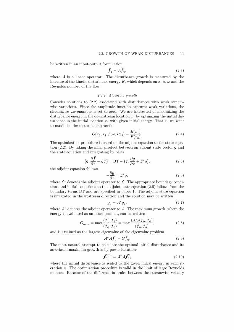
2.3.2. Algebraic growth

Consider solutions to (2.2) associated with disturbances with weak stream-wise variations. Since the amplitude function captures weak variations, thestreamwise wavenumber is set to zero. We are interested of maximizing thedisturbance energy in the downstream location x1 by optimizing the initial dis-turbance in the initial location x0 with given initial energy. That is, we wantto maximize the disturbance growth

G(x0, x1, β, ω,Reδ) =E(x1)

E(x0). (2.4)

The optimization procedure is based on the adjoint equation to the state equa-tion (2.2). By taking the inner product between an adjoint state vector g andthe state equation and integrating by parts

(

g,∂f

∂x− Lf

)

= BT −(

f ,∂g

∂x+ L∗g

)

, (2.5)

the adjoint equation follows

−∂g

∂x= L∗g, (2.6)

where L∗ denotes the adjoint operator to L. The appropriate boundary condi-tions and initial conditions to the adjoint state equation (2.6) follows from theboundary terms BT and are specified in paper 1. The adjoint state equationis integrated in the upstream direction and the solution may be written

g0 = A∗g1, (2.7)

where A∗ denotes the adjoint operator to A. The maximum growth, where theenergy is evaluated as an inner product, can be written

Gmax = max(f1, f1)

(f0, f0)= max

(A∗Af0, f0)

(f0, f0), (2.8)

and is attained as the largest eigenvalue of the eigenvalue problem

A∗Af0 = Gf0. (2.9)

The most natural attempt to calculate the optimal initial disturbance and itsassociated maximum growth is by power iterations

fn+1

0 = A∗Afn

0 , (2.10)

where the initial disturbance is scaled to the given initial energy in each it-eration n. The optimization procedure is valid in the limit of large Reynoldsnumber. Because of the difference in scales between the streamwise velocity


and the velocities in the cross-flow plane, the maximum growth is obtained forinitial disturbances with a zero streamwise component resulting in streamwisestreaks with negligible cross-flow components. Furthermore, a growth that areindependent of Reynolds number can be defined as

G = limRe

δ→∞

G

Re2δ(2.11)

2.3.3. Exponential growth

Consider solutions to (2.2) associated with wave-like disturbances, i.e. where αin the phase function is not equal to zero. As both the amplitude function andthe phase function depend on x, one more equation is required. We requireboth the amplitude function and the wavenumber α to change slowly in thestreamwise direction, and specify a normalization condition on the amplitudefunction

∫ ∞

0

(

u∂u

∂x+

v

Re2δ

∂v

∂x+

w

Re2δ

∂w

∂x

)

dy = 0, (2.12)

where bars denote complex conjugate. The Reynolds number appears due tothe different scaling of streamwise and cross-flow velocities. Other conditionsare possible and are presented in Bertolotti et al. (1992). The normalizationcondition specifies how much growth and sinusoidal variation are representedby the amplitude function and the phase function, respectively. The initialcondition is taken as the least stable eigenfunction from parallel theory withcorresponding eigenvalue α(x0). The exponential growth is maximized in thesense that the envelope of the most amplified eigenmode is calculated.

2.4. Application to the Falkner–Skan boundary layer

In the first paper, the stability of the Falkner–Skan boundary layer to expo-nentially growing waves and non-modal streaks is analyzed. A comparison ofthe algebraic growth with the exponential growth is performed and a unifiedtransition prediction method based on available experimental data is suggested.

2.4.1. Comparison of algebraic and exponential growth

Linear stability analysis is performed with the Falkner–Skan boundary layeras the base flow. The acceleration of the free-stream velocity driven by thepressure gradient is described by the Hartree parameter βH in the formula-tion of a similarity solution. The stability of optimal disturbances and ex-ponentially growing waves are examined for three base flows with favorable,zero and adverse pressure gradients. The corresponding Hartree parametersare βH = 0.1, 0,−0.1. Figure 2.1 shows the stremwise velocity profiles andthe downstream growth of the boundary layer thickness for the three cases.The dashed lines show Blasius boundary layer with zero pressure gradient andtherefore also constant free-stream velocity. The solid lines show the acceler-ated flow with favorable pressure gradient and a thinner boundary layer. The

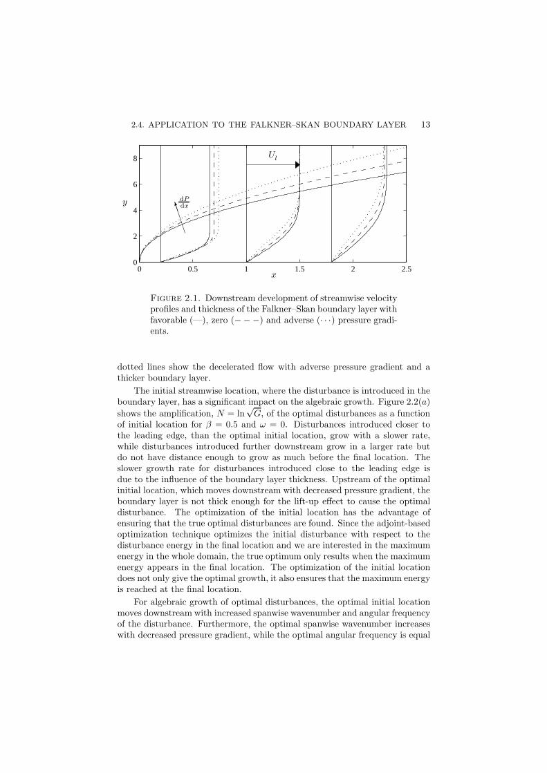
2.4. APPLICATION TO THE FALKNER–SKAN BOUNDARY LAYER 13

0 0.5 1 1.5 2 2.50

2

4

6

8

x

y

Ul

BB

BBMdPdx

Figure 2.1. Downstream development of streamwise velocityprofiles and thickness of the Falkner–Skan boundary layer withfavorable (—), zero (−−−) and adverse (· · ·) pressure gradi-ents.

dotted lines show the decelerated flow with adverse pressure gradient and athicker boundary layer.

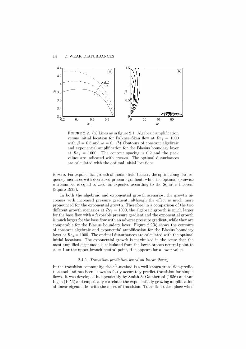
The initial streamwise location, where the disturbance is introduced in theboundary layer, has a significant impact on the algebraic growth. Figure 2.2(a)

shows the amplification, N = ln√G, of the optimal disturbances as a function

of initial location for β = 0.5 and ω = 0. Disturbances introduced closer tothe leading edge, than the optimal initial location, grow with a slower rate,while disturbances introduced further downstream grow in a larger rate butdo not have distance enough to grow as much before the final location. Theslower growth rate for disturbances introduced close to the leading edge isdue to the influence of the boundary layer thickness. Upstream of the optimalinitial location, which moves downstream with decreased pressure gradient, theboundary layer is not thick enough for the lift-up effect to cause the optimaldisturbance. The optimization of the initial location has the advantage ofensuring that the true optimal disturbances are found. Since the adjoint-basedoptimization technique optimizes the initial disturbance with respect to thedisturbance energy in the final location and we are interested in the maximumenergy in the whole domain, the true optimum only results when the maximumenergy appears in the final location. The optimization of the initial locationdoes not only give the optimal growth, it also ensures that the maximum energyis reached at the final location.

For algebraic growth of optimal disturbances, the optimal initial locationmoves downstream with increased spanwise wavenumber and angular frequencyof the disturbance. Furthermore, the optimal spanwise wavenumber increaseswith decreased pressure gradient, while the optimal angular frequency is equal


0 20 40 600

0.5

1

1.5

0.2 0.4 0.6 0.83.2

3.4

3.6

3.8

4

4.2

4.4(a) (b)

x0

N

ω

β�

dPdx

Figure 2.2. (a) Lines as in figure 2.1. Algebraic amplificationversus initial location for Falkner–Skan flow at Reδ = 1000with β = 0.5 and ω = 0. (b) Contours of constant algebraicand exponential amplification for the Blasius boundary layerat Reδ = 1000. The contour spacing is 0.2 and the peakvalues are indicated with crosses. The optimal disturbancesare calculated with the optimal initial locations.

to zero. For exponential growth of modal disturbances, the optimal angular fre-quency increases with decreased pressure gradient, while the optimal spanwisewavenumber is equal to zero, as expected according to the Squire’s theorem(Squire 1933).

In both the algebraic and exponential growth scenarios, the growth in-creases with increased pressure gradient, although the effect is much morepronounced for the exponential growth. Therefore, in a comparison of the twodifferent growth scenarios at Reδ = 1000, the algebraic growth is much largerfor the base flow with a favorable pressure gradient and the exponential growthis much larger for the base flow with an adverse pressure gradient, while they arecomparable for the Blasius boundary layer. Figure 2.2(b) shows the contoursof constant algebraic and exponential amplification for the Blasius boundarylayer at Reδ = 1000. The optimal disturbances are calculated with the optimalinitial locations. The exponential growth is maximized in the sense that themost amplified eigenmode is calculated from the lower-branch neutral point tox1 = 1 or the upper-branch neutral point, if it appears for a lower value.

2.4.2. Transition prediction based on linear theory

In the transition community, the eN -method is a well known transition-predic-tion tool and has been shown to fairly accurately predict transition for simpleflows. It was developed independently by Smith & Gamberoni (1956) and vanIngen (1956) and empirically correlates the exponentially growing amplificationof linear eigenmodes with the onset of transition. Transition takes place when

2.4. APPLICATION TO THE FALKNER–SKAN BOUNDARY LAYER 15

the amplitude of the most amplified disturbance reaches eN times its initial am-plitude. The eN -method does not account for the receptivity process. However,Smith & Gamberoni (1956) and van Ingen (1956) reported, after analyzing datafrom a large number of low-disturbance experiments, that the amplification be-tween 8 and 11 fairly well describes the onset and end of the transition region.They also concluded that those values decrease with increasing free-stream tur-bulence. A modification of the eN -method in order to account for free-streamturbulence was proposed by Mack (1977). The free-stream turbulence levelTu was correlated to the amplification N by comparing the transition Rey-nolds number ReT from experimental flat-plate boundary layer data collectedby Dryden (1959) with parallel linear stability theory for the Blasius boundarylayer. Mack (1977) suggested the following relation for the amplification attransition

N = −8.43 − 2.4 lnTu, (2.13)

which he claimed is valid in the range 0.1 % < Tu < 2 %. For a free-streamturbulence level less than 0.1 %, he mentioned that the dominant disturbancesource is thought to be wind-tunnel noise rather than turbulence.

Andersson et al. (1999) made an attempt at prediction of bypass transitiondue to algebraic growth by correlating the transition Reynolds number and thefree-stream turbulence level

ReTTu = K, (2.14)

where K should be constant for free-stream turbulence levels in the range1 % < Tu < 5 %. By comparison of different experimental studies, the constantwas chosen as K = 12.

Other empirical transition-prediction correlations involving the effects offree-stream turbulence and streamwise pressure gradient have been developed.van Driest & Blumer (1963) postulated that transition occurs when the maxi-mum vorticity Reynolds number reaches a critical value, to be correlated withthe pressure gradient and free-stream turbulence level. In the case of zero pres-sure gradient, their formula correlated with experiments agrees well with (2.14).Another example is a model of Abu-Ghannam & Shaw (1980), which gives theReynolds number based on the momentum thickness θ, at the start and endof the transition region. The only inputs to the model are the free-stream tur-bulence level and the pressure gradient parameter λθ = (θ2/ν)∂Ul/∂x. Moreadvanced transition prediction and studies of the transition phenomena itselfcan be made by numerical simulations such as the nonlinear PSE technique(e.g. Hein et al. 1999) and DNS.

The transition model of Andersson et al. (1999) can be complemented withthe addition of base flows with various pressure gradients. The model is basedon three assumptions.

1. Assume that the initial disturbance energy is proportional to the free-stream turbulence energy

E(x0) ∝ Tu2, (2.15)


for isotropic turbulence with the free-stream turbulence level defined as

Tu =√

u′2/Ul. Here u′ is the fluctuating streamwise velocity in thefree stream and the overbar denotes the temporal mean.

2. Assume that the initial disturbance grows with the optimal rate

E(x1) = GE(x0) = GRe2δE(x0). (2.16)

3. Assume that transition occurs when the final energy reaches a specificvalue ET , regardless of the pressure gradient of the base flow

E(x1) = ET . (2.17)

Combining assumptions (2.15–2.17) yields the transition model

ReTTu =k√G, (2.18)

where k should be constant. Using the same correlation as Andersson et al.

(1999) and the optimal growth in the Blasius boundary layer gives k = 0.70.This model differs from the one of Andersson et al. (1999) in the sense thatthe growth is optimized over the initial location and the disturbances does notevolve from the leading edge.

The influence of free-stream turbulence on the generation of TS-waves isnot conclusive. In fact, Boiko et al. (1994) made experiments on the behaviorof controlled TS-waves, introduced by means of a vibrating ribbon, in a bound-ary layer subjected to Tu = 1.5 %. The measured amplification rates for thewaves in the presence of the turbulence generating grid were smaller than forregular TS-waves, and damping set in further upstream than in the absenceof the turbulence generating grid. Thus, we make the simple assumption thattransition resulting from exponentially growing disturbances occurs at N = 8,the dashed line in figure 2.3(a), irrespective of the free-stream turbulence level.

Figure 2.3(b) shows the transition Reynolds number based on the resultsfrom the linear stability analysis and the transition model discussed above forfree-stream turbulence. The straight part of the lines represents the transitionReynolds number for exponentially growing modal disturbances and the curvedpart represents bypass transition. For high free-stream turbulence levels, tran-sition occurs as a result of the breakdown of streaky structures and for lowfree-stream turbulence levels as a result of exponentially growing disturbances.The cross-over point occurs where the bypass-transition model predicts a highertransition Reynolds number than for the exponentially growing disturbances.According to the model, bypass transition occurs in the Blasius boundary layer(dashed lines) for a free-stream turbulence level higher than 0.76 %. Similarresults have been found in experiments. Suder et al. (1988) found in their ex-periment that the bypass mechanism prevailed for free-stream turbulence levelsof 0.65 % and higher. Kosorygin & Polyakov (1990) suggested that TS-wavesand streaks can coexist and interact for free-stream turbulence levels up toapproximately 0.7 %. However, the model does not account for the interactionbetween TS-waves and streaks.

2.5. APPLICATION TO BOUNDARY LAYERS WITH WALL SUCTION 17

103

0

1

2

3

4

5

6

0.5 1 1.5 2 2.5 3

2

4

6

8(a) (b)

Tu

N

ReT

Tu�

��+dPdx

Figure 2.3. (a) Predicted amplification at transition versusfree-stream turbulence level given in percent for algebraic (—)and exponential (−−−) growth. Model of Mack (1977) (· · ·).(b) Lines as in figure 2.1. Predicted transition contour in theReT -Tu plane with the turbulence level given in percent. Ex-perimental data for the Blasius boundary layer from Matsub-ara & Alfredsson (2001) (M) and Roach & Brierley (1992) (◦).Numerical data from Yang & Voke (1991) (

�).

2.5. Application to boundary layers with wall suction

In the second paper, a comparison of the algebraic growth of spatially devel-oping streaks in the asymptotic suction boundary layer and the semi suctionboundary layer is done. The difference between spatial and temporal theory isalso considered.

2.5.1. Suction boundary layers

In the boundary-layer experiment of Fransson & Alfredsson (2003), suction wasapplied through a plate of porous material. However, the leading-edge part ofthe flat plate was made of an impermeable material allowing the boundary layerto develop and grow downstream until it reaches the porous plate. Downstreamof this position, the flow undergoes an evolution from the Blasius profile towardsthat of the asymptotic suction boundary layer, which have a constant boundarylayer thickness. The semi suction boundary layer, where uniform suction isapplied from the distance l downstream of the leading edge of a flat platecan be calculated with the boundary-layer equations. Figure 2.4 shows thedisplacement thickness of the calculated flow compared with measurementsfrom Fransson & Alfredsson (2003). In order to avoid a discontinues jump inthe suction rate with a corresponding kink in the development of the boundarylayer thickness, the suction is smoothly increased from zero to its full valueover a short distance, see the zoom-up in figure 2.4. On the right-hand side offigure 2.4, the profile of the asymptotic suction boundary layer is shown. It is


0 1 2 3 4 5 6 7 80

0.5

1

1.5

2

2.5

3

3.5

4

y

x

U

δ1

��7

Figure 2.4. Calculated displacement thickness of the semisuction boundary layer compared with measurements (•) fromFransson & Alfredsson (2003). The zoom-up shows the start-ing position of abruptly (− − −) and smoothly (—) appliedsuction. On the right-hand side, the profile of the asymptoticsuction boundary layer is shown.

an analytical solution to the Navier–Stokes equations and can be written as

U(y) = U0 [1 − exp(−y∗V0/ν)] , V = −V0, (2.19)

where y∗ is the dimensional wall-normal coordinate and −V0 is the suctionvelocity. The analytical solution allows the displacement thickness to be calcu-lated exactly, δ1 = ν/V0, and the Reynolds number based on the displacementthickness to be expressed as the velocity ratio, Reδ

1

= U0/V0. Thus, for this

flow it is natural to use the displacement thickness as the length scale. However,if we choose l = Reδ

1

δ1 it follows that δ = δ1 and accordingly Reδ = Reδ1

. In

the experiment of Fransson & Alfredsson (2003), the suction was applied from360 mm downstream of the leading edge and the suction Reynolds number wasReδ

1

= 347.

2.5.2. Algebraic growth

Fransson & Corbett (2003) performed temporal stability analysis of the as-ymptotic suction boundary layer and compared the spanwise scales of optimallygrowing streaks with those observed in the experiment of Fransson & Alfredsson(2003). Here, a twofold improvement is done by performing a spatial stabil-ity analysis of the semi suction boundary layer. Fransson & Corbett (2003)

2.5. APPLICATION TO BOUNDARY LAYERS WITH WALL SUCTION 19

−30 −20 −10 0 10 20 300

5

10

−30 −20 −10 0 10 20 300

5

10

15

20

−30 −20 −10 0 10 20 300

5

10

15

20

25

(a)

(b)

(c)

y

y

y

z

Figure 2.5. Optimal disturbances in the semi suction bound-ary layer at Reδ

1

= 347. (a) 0 ≤ x ≤ 2. (b) 0 ≤ x ≤ 6.

(c) 0 ≤ x ≤ 10.

found that the optimal disturbance has the spanwise wavenumber β = 0.53.With spatial analysis, the optimal growth is 16 % higher corresponding to adisturbance with spanwise wavenumber β = 0.52.

The suction boundary layers are studied over nine streamwise intervals,starting at x0 = 0 and with suction from x = 1 to the end of the interval. Thelength of the interval is varied by changing the end position from x1 = 2 tox1 = 10 in steps of one. The optimal disturbance at the initial position takesthe form of streamwise aligned vortex pairs, as seen in figure 2.5, which showsthe optimal disturbances in the semi suction boundary layer at Reδ

1

= 347 for

three intervals. It can be seen that the vortex cores of the optimal disturbancemove upward and the vortices grow in size when the streamwise interval isprolonged. Thus, the optimal spanwise wavenumber decreases as the intervalis prolonged. Furthermore, the corresponding optimal growth decreases withincreased interval and the optimal angular frequency is zero.


0 0.5 10

0.5

1

x 10−3

0 0.5 10

1

2

3

4

x 10−4

0 0.5 10

1

2

x 10−4

0 0.5 1 1.5 20

0.5

1

1.5

x 10−3

0 2 4 60

2

4

x 10−4

0 5 100

1

2

x 10−4

(a) (b)

(c) (d)

(e) (f)

G

G

G

β x

Figure 2.6. Comparison of algebraic growth in the asymp-totic suction boundary layer (− − −) and the semi suctionboundary layer (—) at Reδ

1

= 347. (a, b) 0 ≤ x ≤ 2.

(c, d) 0 ≤ x ≤ 6. (e, f) 0 ≤ x ≤ 10.

Figure 2.6 shows a comparison of the optimal growth versus spanwisewavenumber and streamwise coordinate, with the optimal spanwise wavenum-ber, between the semi suction boundary layer and the asymptotic suctionboundary layer. It reveals that for the shortest interval, the semi suctionboundary layer gives a 25 % higher optimal growth than for the asymptoticsuction boundary layer. The optimal growth also occurs at a lower spanwisewavenumber. Studying the growth as function of streamwise coordinate, weconclude that the reason for the difference in growth is the contribution fromthe Blasius profile at the beginning of the interval. However, the differences ingrowth and optimal spanwise wavenumber decrease as the interval is prolonged.

2.6. APPLICATION TO THE BLASIUS WALL JET 21

2.6. Application to the Blasius wall jet

In the third paper, the Blasius wall jet is constructed and matched to anexperimental set-up. The stability of the flow to eigenwaves and non-modalstreaks is analyzed and compared to the experiments.

2.6.1. Comparison of linear theory with experiments

Linear stability analysis is performed with the Blasius wall jet as the baseflow. The stability of optimal disturbances and exponential growing waves isexamined and compared to measurements performed in the wall-jet facility atChalmers University of Technology. The base flow is matched to the experi-ment with the maximum outlet velocity U0 = 15.4 m s−1, corresponding to theReynolds number Reδ = 173. Due to growing boundary layers in the experi-mental nozzle, a virtual slot is placed the distance l = 29 mm upstream of theexperimental nozzle opening and the virtual slot height is b∗ = 2.06 mm cor-responding to the non-dimensional value b = 12.3. A comparison of the baseflow with the measured hot-wire data is shown in figure 2.7(a). The agree-ment increases downstream of the nozzle opening. The largest disagreementis observed in the upper part of the wall jet. This is due to a jump of theboundary conditions that occur on the top lip of the nozzle as the flow leaves,resulting in a kink of the experimental velocity profile. However, with increaseddownstream distance, the influence of the nozzle disappears.

The stability analysis reveals a very high instability of the flow to two-dimensional eigenmodes and a rather high instability to non-modal streaks.The waves are triggered by a loudspeaker in the experiment and the frequencywas chosen close to the natural dominating flow frequency, namely 1221 Hzcorresponding to ω = 14.4. Both in the experiment and in the computation,the most amplified frequency decreases with increased streamwise location.Figure 2.7(b) shows a comparison of the computed streamwise amplitude dis-tribution and the measurement at the location x = 1.55. The measurementwas performed with three different forcing amplitudes, 0.3 %, 1.1 % and 1.7 %,measured at x = 1.55, and the agreement in the results between the differentforcing amplitudes indicates the linearity of the disturbance. The disturbancehas a very typical shape and the peak in the shear-layer region is in antiphaseto the peak near the wall. The deviation between the linear stability analysisand the experiment in the upper part of the wall jet is because the waves in theexperiment are not fully developed eigenmodes so close to the nozzle opening,however, the agreement improves downstream.

The computed optimal disturbance consists of streamwise vortices devel-oping into streamwise streaks. Between two vortices, the flow is either movingupward or downward. Where the flow is moving upward between two vortices,high-momentum fluid is moved up from the jet core, producing a high-velocitystreak in the shear-layer region of the wall jet. In the boundary-layer region,a weak low-velocity streak is formed below the high-velocity streak, since theupward motion of fluid there carries low-momentum fluid from the wall region.


0 0.5 10

5

10

15

20

25

30

0 0.5 10

5

10

15

20

25

30

0 0.5 10

5

10

15

20

25

30(a) (b) (c)

U |u| |u|

y

Figure 2.7. Comparison of computations (—) and measure-ments of the Blasius wall jet at x = 1.55 for Reδ = 173.The disturbance amplitudes are normalized with their max-imum value. (a) Computed and measured (◦) base flow.(b) Streamwise wave amplitude for ω = 14.4. The disturbanceare triggered in the experiment by a loudspeaker and have theamplitudes 0.3 % (◦), 1.1 % (

�) and 1.7 % (M). (c) Streamwise

streak amplitude. The optimal disturbance are calculated forβ = 0.211, ω = 0, x0 = 0.403 and x1 = 1.55. The experimen-tal results are taken from three spanwise scales correspondingto β = 0.176 (◦), β = 0.218 (

�) and β = 0.264 (M).

The opposite motion results, half a wavelength away, where the flow is movingdownward between two vortices, producing a low-velocity streak in the shear-layer region and a weak high-velocity streak in the boundary-layer region. Infigure 2.7(c), the resulting normalized streak from the optimal disturbance,calculated for β = 0.211, ω = 0, x0 = 0.403 and x1 = 1.55 is compared withthe measured streaks with spanwise scales β = 0.264, 0.218 and 0.176. In theexperiment, the streaks are introduced in the flow by periodically distributedroughness elements that are located onto the top lip of the nozzle. Both in thecomputation and in the experiment, the streak remains very similar for differ-ent spanwise wavenumber β. The same is true in the computation for differentinitial location, x0.

CHAPTER 3

Strong disturbances

3.1. Numerical method and disturbance generation

In the present chapter as well as the next one, all simulations of the flowsare performed by solving the Navier–Stokes equations directly. That is, theequations governing incompressible fluid motion are numerically solved withoutany simplifying assumptions. This requires that all the relevant scales of theflow must by resolved and results in large computational efforts, both in termsof memory and effective time of the calculation.

The in-house numerical code at KTH Mechanics (Lundbladh et al. 1999)uses spectral methods to solve the three-dimensional time-dependent incom-pressible Navier–Stokes equations. All velocities and lengths are scaled by thefree-stream velocity and the displacement thickness at the inlet of the compu-tational box, respectively. The time, frequency and wavenumbers are scaledcorrespondingly. The discretization in the streamwise and spanwise directionsmakes use of Fourier series expansions, which enforces periodic solutions. Thediscretization in the wall-normal direction is represented with Chebyshev poly-nomial series. A pseudospectral treatment of the nonlinear terms is used. Thetime advancement used is a second-order Crank–Nicolson method for the lin-ear terms and a four-step low-storage third-order Runge–Kutta method for thenonlinear terms. Aliasing errors arising from the evaluation of the convectiveterms are removed by dealiasing by padding and truncation using the 3/2-rulewhen the FFTs are calculated in the wall-parallel planes. In the wall-normaldirection, it has been found that increasing the resolution is more efficient thanthe use of dealiasing.

At the wall, a no-slip boundary condition is specified and at the upperboundary, a generalized boundary condition is applied in Fourier space withdifferent coefficients for each wavenumber. The condition represents a poten-tial flow solution decaying away from the upper edge of the computational box.This condition decreases the required box height by damping the higher fre-quencies rather than forcing the disturbance velocities to a rapid decay. In thehorizontal directions, periodic boundary conditions are used.

For spatially growing flows such as the Falkner–Skan boundary layer andthe Blasius wall jet, a fringe region (Nordstrom et al. 1999) is added in thedownstream end of the computational domain to fulfill the necessary periodic

23

24 3. STRONG DISTURBANCES

boundary condition in the streamwise direction, required by the spectral dis-cretization. In this region, the flow is smoothly forced to the desired inflowsolution. When studying parallel flows, such as the asymptotic suction bound-ary layer with periodic or localized disturbances, the advantage of omitting thefringe region can be used.

The present numerical implementation provides several possibilities for dis-turbance generation. Disturbances can be included in the flow by a body force,by blowing and suction at the wall through non-homogeneous boundary condi-tions and by adding them in the initial velocity field. When a fringe region ispresent, disturbances can be forced in it and thereby be included in the desiredinflow solution.

3.2. DNS of the Blasius wall jet

In the third paper, waves and streaks are introduced in the Blasius wall jet andthe nonlinear interaction and transition process are studied by means of DNS.

3.2.1. Spectral analysis

Waves and streaks from the linear stability calculations (figure 2.7) are excitedin the DNS. The amplitudes, which are chosen to obtain a similar transitionscenario as in the experiment, are prescribed in the beginning of the computa-tional box to 0.1 % and 3 % of the wall-jet core velocity, respectively.

A convenient way to study the nonlinear interaction between the wavesand the streaks is to look at the energy development of the Fourier componentsshown in figure 3.1. The velocity components are Fourier transformed in timeand in the spanwise direction and (ω1, β1) denotes the frequency and spanwisewavenumber, each normalized with the corresponding fundamental frequencyand wavenumber. Thus, the waves and the streaks are represented by (1, 0)and (0, 1), respectively, and are shown as black solid lines. Before nonlinearinteraction sets in, the modes amplify in agreement with the linear theory asobserved in the beginning of the computational box, where the waves growexponentially and the streaks have an algebraic growth. The results fromthe PSE are shown as circles and the agreement is excellent. Close to thenozzle opening, the two-dimensional effects are dominating over the strongerforced stationary streaks. At about x = 30 to 40, nonlinear effects begin tobe apparent when energy is transferred to the modes (1, 1), (2, 0) and (2, 1).Further downstream, the streak mode (0, 1) is decaying and a dip in the energycan be observed at approximately x = 55. At this location, the wave mode (1, 0)starts to saturate and an abrupt change of the breakdown process happens,namely, an exponential growth of the streak mode.

Flows such as free shear layers and wall jets can undergo pairing of thefundamental vortex rollers as a result of a subharmonic instability. In order toasses whether the pairing mode (1/2, 0) is present in the simulation, the energycontent in this subharmonic frequency is evaluated and shown as the gray linein figure 3.1. However, since this mode is not forced (in the fringe region),

3.2. DNS OF THE BLASIUS WALL JET 25

0 20 40 60 80 100 12010

−6

10−4

10−2

100

x

E (0, 1)

(1, 0)

(1, 1)

(2, 0)

-(2, 1)

HHHHY

(0, 2)HHHHY

(1, 2)(2, 2)

� (1/2, 0)

Figure 3.1. Energy in different Fourier modes (ω1, β1) fromthe DNS. Initially excited wave and streak modes (black solidlines). Nonlinearly generated modes (dashed and dotted lines).Pairing mode (gray line) grows up from numerical noise. Re-sults from the PSE (◦) are shown for comparison.

but only grows out of numerical noise, its amplitude is small. Upstream ofthe location where nonlinear interactions set in, the amplification rate of thesubharmonic mode is about half of the fundamental one. This is consistentwith linear theory, indicating that an eigenmode is born. At about x = 55, theamplification rate doubles as a result of nonlinear effects. However, the energycontent in this mode stays at least one magnitude below the exponentiallygrowing streak mode.

3.2.2. Flow structures

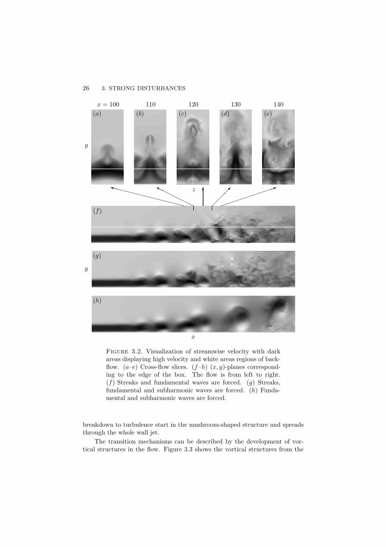
Structures appearing in the flow can be visualized and contribute to an in-creased understanding of the transition process. In figure 3.2, the streamwisevelocity is visualized, where dark areas display high velocity and white areasshow regions of backflow. Figures 3.2(a–e) show cross-flow slices from stream-wise locations indicated in the figure. The high-velocity streak is lifted up fromthe shear-layer region forming a mushroom-shaped structure. Such structureshave also been observed by, for example, Wernz & Fasel (1996, 1997) and Gogi-neni & Shih (1997). Figure 3.2(f) shows the (x, y)-plane through the middleof the low-velocity streak (the edges of the cross-flow slices). Counterclockwiserotating rollers are moving with the wave troughs in the outer shear layer.Slightly downstream of each shear-layer roll-up, clockwise rotating rollers inthe boundary layer exist, associated with small regions of separated flow. The


x = 100 110 120 130 140

(a) (b) (c) (d) (e)

y

z

XXXXXXXXXXXXy

HHHHHHY 6

��

��

��1

(f)

(g)

(h)

y

x

Figure 3.2. Visualization of streamwise velocity with darkareas displaying high velocity and white areas regions of back-flow. (a–e) Cross-flow slices. (f–h) (x, y)-planes correspond-ing to the edge of the box. The flow is from left to right.(f) Streaks and fundamental waves are forced. (g) Streaks,fundamental and subharmonic waves are forced. (h) Funda-mental and subharmonic waves are forced.

breakdown to turbulence start in the mushroom-shaped structure and spreadsthrough the whole wall jet.

The transition mechanisms can be described by the development of vor-tical structures in the flow. Figure 3.3 shows the vortical structures from the

3.2. DNS OF THE BLASIUS WALL JET 27

x

y

z

Figure 3.3. Vortex visualization using the same instanta-neous data as in figures 3.2(a–f)

same instantaneous data as the visualizations shown in figures 3.2(a–f). Span-wise rollers are formed in the wave troughs in the outer shear layer and movedownstream. In the boundary layer close to the wall beneath the wave crests,counter-rotating rollers are formed. In the presence of streaks, the shear-layerrollers are sinuously modified with the boundary-layer rollers deforming in theopposite direction. Vortex ribs are formed in the braids of the waves, extendingfrom the top of the shear-layer roller to beneath the previous one. Such rib vor-tices have been observed in many experimental and computational studies ofmixing layers (e.g. Bernal & Roshko 1986; Lasheras et al. 1986; Metcalfe et al.

1987; Schoppa et al. 1995). The vortex ribs follow the upward flow between twoneighboring shear-layer rollers and are associated with the mushroom-shapedstructures ejected from the wall jet into the ambient flow. The tail legs ofthe vortex ribs, generated one fundamental period earlier, separate and form avortex ring around the upcoming vortex ribs and additional counter-rotatingvortex rings are created preceding breakdown to turbulence.


3.2.3. Subharmonic waves and pairing

The primary instability in inflectional base flows such as free shear layers andwall jets is a strong inviscid exponential instability resulting in the roll-upof waves into strong spanwise vortices. These two-dimensional vortices canexperience two different types of secondary instability. For low initial three-dimensional excitation, the secondary instability is subharmonic and associatedwith vortex pairing, like that observed by Bajura & Catalano (1975). If theinitial three-dimensional excitation is large enough, a three-dimensional sec-ondary instability is predominant, which suppresses the vortex pairing (see e.g.Metcalfe et al. 1987).

In order to determine the role of pairing in the Blasius wall jet, the sub-harmonic disturbance is studied. The Orr–Sommerfeld mode with half thefrequency of the fundamental one is forced in the DNS. Apart from the simula-tion showed in figure 3.2(f), where streaks and fundamental waves are excited,two additional simulations are performed, one with streaks, fundamental andsubharmonic waves forced in the flow (figure 3.2g) and the other with only thefundamental and subharmonic waves and noise in the initial field (figure 3.2h).When the subharmonic waves are not forced, the pairing mode is weak, as isalso seen in the energy content of the corresponding Fourier mode (1/2, 0) infigure 3.1. In this case pairing does not occur. On the other hand, when thesubharmonic waves are forced, the pairing mode is stronger and can be seenas the staggered pattern of the vortex rollers in the outer shear layer. In theabsence of streaks, pairing occurs between rollers in the outer shear layer aswell as in the boundary layer. The pairing originates from the subharmonicwave displacing one vortex to the low-velocity region and the next to the high-velocity region. The vortex traveling in the high-velocity region overtakes theslower vortex in the low-velocity region, and pairing appears. However, inthe presence of streaks, pairing is suppressed and breakdown to turbulence isenhanced.

3.3. DNS of the asymptotic suction boundary layer

The numerical code does not allow for non-zero mean mass flow through thelower and upper boundaries. However, the wall-normal suction in the asymp-totic suction boundary layer can be moved from the boundary condition to thegoverning equations. Hence, instead of solving the Navier–Stokes equations forthe wall-normal velocity V with the boundary condition V = −V0, the samesolution can be obtained by solving for V − V0 with the boundary conditionV = 0.

3.3.1. Energy thresholds for periodic disturbances

In the fourth paper, energy thresholds for bypass transition in the asymptoticsuction boundary layer are studied by means of DNS. The growth and break-down of streaks triggered by streamwise vortices (SV) and oblique waves (OW)are investigated as well as the development of random noise (N).

3.3. DNS OF THE ASYMPTOTIC SUCTION BOUNDARY LAYER 29

Three transition scenarios are investigated where the disturbances are in-troduced in the initial field and allowed to evolve temporally. Because the dist-urbances are assumed to be periodic in the horizontal directions and the baseflow is parallel, the fringe region can be omitted. In scenario (SV), the initialflow field consists of two counter-rotating streamwise vortices. These vorticesproduce streaks by the lift-up effect as time proceeds. Transition can take placeif the streak amplitude becomes sufficiently large for secondary disturbancesto amplify and break down. In scenario (OW), the initial flow field consists oftwo superposed oblique waves with equal and opposite angle to the streamwisedirection. The pair of growing waves interact nonlinearly and streamwise vor-tices are created. This is essentially a different and quicker way of triggeringgrowth of streaks, which in turn are subjected to secondary instability. Thestreamwise vortices and oblique waves are added in the form

u = u(y) exp(iαx+ iβz), (3.1)

where the amplitude function u(y), with given horizontal wavenumbers (α, β),is optimized over a specified time period (Corbett & Bottaro 2000; Frans-son & Corbett 2003). In scenario (N), the initial flow field consists of three-dimensional random noise added to the base flow. The thresholds for transitionare expressed in terms of the energy density of the initial disturbance, thus theinitial disturbance energy E0 divided by the volume � of the computationalbox.

The streamwise vortices are optimized for (α, β) = (0, 0.53) over a timeperiod of 300. The horizontal lengths of the computational box are 2π/β, whichcorresponds to one spanwise wavelength of the optimal disturbance. Apartfrom the streamwise vortices, the initial condition consists of a small amountof random noise, which is necessary to set off a secondary instability. Theflow pattern of the simulation for Re = 800 and E0/� = 3 · 10−5 is shownin figure 3.4(a, b), where the streamwise velocity is visualized in a horizontalplane (with two box lengths in each direction) at y = 2. As can be seenin figure 3.4(a) that shows the state at t = 700, a secondary instability hasdeveloped and deforms the streaks in a sinuous manner with a streamwisewavelength equal to the computational box length. Figure 3.4(b) shows thebreakdown of the streaks at t = 820.

The oblique waves are optimized for (α, β) = (0.265,±0.265) over a timeperiod of 75. Hence, they are oriented 45◦ to the free-stream direction. Thehorizontal lengths of the computational box are twice as large as for scenario(SV) in order to fit one streamwise and spanwise wavelength of the obliquewaves. The same random noise as for scenario (SV) is added to the initialfield, although it is not necessary for secondary instability to occur. The flowpattern of the simulation for Re = 800 and E0/� = 1 · 10−5 is shown infigure 3.4(c, d), where the size of the horizontal plane at y = 2 is equal to thehorizontal size of the computational box. In the initial stage, the pair of obliquewaves interact with each other and streamwise vortices with half the spanwisewavelength are created. As a result, two spanwise wavelengths of streaks can


(a) (b)

(c) (d)

x x

z

z

Figure 3.4. Visualization of periodic disturbances in the as-ymptotic suction boundary layer for Re = 800 in a horizontalplane at y = 2 of size: 23.71 × 23.71. Dark and light areasshow regions of high and low streamwise velocity, respectively,and the flow is from left to right. Scenario (SV) at (a) t = 700and (b) tT = 820. Scenario (OW) at (c) t = 600 and(d) tT = 731.

be seen in figure 3.4(c) that shows the state at t = 600. In the presence of theoblique modes, the secondary instability is of the varicose type with horizontalwavelengths equal to these of the oblique waves, and thus also of the horizontaldimensions of the computational box. Figure 3.4(d) shows the breakdown ofthe streaks at t = 731.

The Reynolds number based on the mean friction velocity, Reτ , provides agood measure of when transition to turbulence appears. Transition is defined toappear when the friction velocity Reynolds number exceeds a certain criticalvalue. This value is chosen to be 26, 38 and 50 for Reynolds number 500,800 and 1200, respectively. Examples of the evolution of the friction velocityReynolds number are shown in figure 3.5(a), which shows one case from each


0 500 1000

30

35

40

45

0 500 1000 1500 2000

10−5

10−4

10−3

103

10−6

10−4

(a) (b)

(c)

Re tT

E0/�

t

Reτ

E0/�

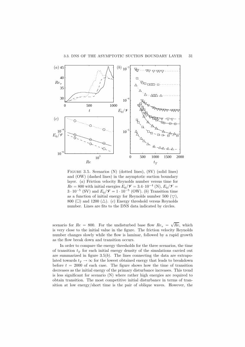
Figure 3.5. Scenarios (N) (dotted lines), (SV) (solid lines)and (OW) (dashed lines) in the asymptotic suction boundarylayer. (a) Friction velocity Reynolds number versus time forRe = 800 with initial energies E0/� = 3.4 ·10−4 (N), E0/� =3 · 10−5 (SV) and E0/� = 1 · 10−5 (OW). (b) Transition timeas a function of initial energy for Reynolds number 500 (5),800 (�) and 1200 (4). (c) Energy threshold versus Reynoldsnumber. Lines are fits to the DNS data indicated by circles.

scenario for Re = 800. For the undisturbed base flow Reτ =√Re, which

is very close to the initial value in the figure. The friction velocity Reynoldsnumber changes slowly while the flow is laminar, followed by a rapid growthas the flow break down and transition occurs.

In order to compare the energy thresholds for the three scenarios, the timeof transition tT for each initial energy density of the simulations carried outare summarized in figure 3.5(b). The lines connecting the data are extrapo-lated towards tT → ∞ for the lowest obtained energy that leads to breakdownbefore t = 2000 of each case. The figure shows how the time of transitiondecreases as the initial energy of the primary disturbance increases. This trendis less significant for scenario (N) where rather high energies are required toobtain transition. The most competitive initial disturbance in terms of tran-sition at low energy/short time is the pair of oblique waves. However, the


−25 −20 −15 −10 −5 0 5 10 15 20 25−15

−10

−5

0

5

10

15

z

x

Figure 3.6. Contours of wall-normal velocity, at y = 1, of alocalized disturbance consisting of two counter-rotating vortexpairs with the scales lx = 10, ly = 1.0 and lz = 5.5. Black andgray lines display positive and negative values, respectively.

obtained energy thresholds must be considered as an upper bound, since onlyone disturbance configuration is simulated in each case.

It is difficult to define the energy threshold as a function of Reynolds num-ber for growing boundary layers as the local Reynolds number changes with theboundary layer thickness. In parallel flows, however, such as the asymptoticsuction boundary layer, the Reynolds number based on the boundary layerthickness is constant and therefore the procedure to find the energy thresh-old is straightforward. The energy thresholds for transition, extracted fromfigure 3.5(b) (where the lines approach the time 2000), are plotted for theirrespective Reynolds number in figure 3.5(c). The values from the DNS aredisplayed by circles and the lines represent least square fits of the formulaE0 ∝ Reγ . The obtained energy thresholds for the three transition scenariosscale with Reynolds number as Re−2.6 (OW), Re−2.1 (SV) and Re−2.1 (N).

3.3.2. Amplitude thresholds for localized disturbances

In the fifth paper, amplitude thresholds for transition from localized distur-bances to turbulent spots are studied with DNS. The localized disturbanceis superposed to the asymptotic suction boundary layer in the initial velocityfield. The type of disturbance is centered around a pair of oblique waves, inthe streamwise-spanwise wavenumber plane, consisting of two counter-rotatingvortex pairs, see figure 3.6. In terms of a stream function, it is defined by

ψ = Axy3z exp (−x2 − y2 − z2), (3.2)


Figure 3.7. A growing localized disturbance in the asymp-totic suction boundary layer. Typical vortex structures (green)are visualized together with their associated velocity normalto the wall (red indicating upward moving fluid and blue fluidmoving downward). The dark regions at the wall show areasof increased friction.

where x = x/lx, y = y/ly and z = z/lz. The velocity components are given by(u, v, w) = (0,−ψz, ψy) and normalized so that the amplitude A is given by themaximum absolute value of the wall-normal disturbance velocity. This type ofinitial disturbance can be experimentally reproduced with the down-up motionof a membrane at the wall and has been used in earlier studies of transientgrowth and transition in channel flows (Henningson et al. 1993) and boundarylayers (Breuer & Haritonidis 1990; Breuer & Landahl 1990; Bech et al. 1998).

The initial disturbance develops into a hairpin vortex aligned with thestreamwise direction. Its legs are close to the wall at the trailing edge ofthe disturbance while the head is located higher up and further downstream.Between the legs, an upward motion is present. On each side of the head,counter-rotating structures develop. Figure 3.7 shows an instant of a developinglocalized disturbance and the friction distribution at the wall (the figure wasoriginally prepared for the book ‘KTH in Your Pocket 2005’ and appears on itscover). The head is detached as a result of vortex stretching and a new head isformed in its place. This head detachment continues as time proceeds. Spiralvortices appear at the counter-rotating structures on each side. Later, the flowpattern becomes complex with many hairpin and spiral vortices characterizinga young turbulent spot.

Amplitude thresholds for transition from a localized disturbance to a tur-bulent spot is investigated by a numerous of direct numerical simulations. Ifthe initial amplitude of the disturbance exceeds a certain threshold value, AT ,transition occurs. Simulations are carried out with varied initial amplitudes ofthe localized disturbance at the Reynolds numbers 500, 800 and 1200. Whenevaluating whether transition occurs or not, the disturbance energy, extremevalues of velocity and vorticity components and visual examinations of the


0 500 10000

10

20

30

40

50

103

100

101

(a) (b)

E

t

AT

Re

Figure 3.8. (a) Evolution of disturbance energy at Re =500 and A = 0.046 (solid line), 0.045 (dashed line) and 0.044(dotted line). (b) Threshold amplitude as function of Reynoldsnumber. The circles correspond to the lowest amplitudes fromthe DNS that lead to transition. The black line is a least squarefit to the data corresponding to AT = 6.36 · 104Re−1.54. Thegray line indicates the critical Reynolds number of 367.

flow field are taken into account. Figure 3.8(a) shows the evolution of thedisturbance energy for three initial amplitudes close to the threshold value atRe = 500. In this case, transition occurs for the amplitudes A = 0.045 and0.046 but not for 0.044 for which the disturbance energy and flow extremevalues decay after the initial transient growth.

The circles in figure 3.8(b) summarizes the amplitude thresholds takenas the lowest amplitudes for which transition is attained in the DNS beforet = 1000 for the three Reynolds numbers. The black line is the least square fitto the data and for this range of Reynolds numbers, the threshold amplitude isfound to scale asRe−1.5. An attempt of finding the critical Reynolds number fortransition initiated of the localized disturbance is also carried out. Simulationsare performed with an initial amplitude of the localized disturbance of 0.1 andvaried Reynolds numbers. Relaxation of the localized disturbance appears forRe = 367 or below. This value is indicated in figure 3.8(b) as the thick grayline.

CHAPTER 4

Turbulence

4.1. The essence of turbulence

As was mentioned in the Introduction, turbulent flow is characterized by achaotic, swirly and fluctuating motion, like the white jet of water from thekitchen tap. Turbulence is unpredictable in its nature, because a very smalldifference in the initial conditions, causes a completely different solution at alater instant. An example of this sensitivity on initial conditions is the Butter-fly Effect, an expression coined after the work by Lorenz (1963), that the flapof a butterfly’s wings will create a disturbance that in the chaotic motion ofthe atmosphere will become amplified and eventually change the weather. Asa result, it is impossible to predict the weather, one can only compute possi-ble outcomes of how the weather will be. That is actually what is done, themeteorological institutes perform one simulation with initial conditions basedon weather observations, then additional simulations are done with slightlydisturbed initial conditions in order to test the sensitivity and thereof the reli-ability of the forecast.

If we consider the white turbulent flow from the kitchen tap again, and takea photograph with a very short shutter time, we will see a picture of all thefluctuations with lots of small bubbles in it. If we take one more photograph, itwill look different. On the other hand, if we take a photograph with a very longshutter time, we will see a diffusive smooth picture showing the mean behaviorof the jet of water. Now we do not need to take another photograph, becauseit will look the same. In applications one is not usually interested in knowingall the details about the fluctuations of the flow, but rather satisfied with theinfluence of the turbulence on the averaged flow. For this purpose we dividethe total flow into an average and a fluctuating component

ui = Ui + u′i, p = P + p′, (4.1)

where Ui denotes the mean velocity and u′i the fluctuation. The index denoteseither one of the three spatial directions. As well as one can take the averagein time, as the photograph taken with a very long shutter time, one can takethe average in either of the spatial directions what ever is convenient for theparticular flow case. In the case of the jet of water, it is convenient to averagein time and in the azimuthal direction, but not in the streamwise or the radialdirections.

35

36 4. TURBULENCE

By introducing (4.1) into the Navier–Stokes equations and taking the av-erage, we receive the Reynolds average equations governing the mean flow.These equations include the effect of the turbulence through the Reynoldsstress u′iu

′j, where the line denotes average. Because of this additional stress,

the Reynolds average equations involve more unknowns than equations and cannot be solved directly. This closure problem implies that the Reynolds stresscomponents have to be modeled and thereof be expressed in the mean flowvariables. However, in the present thesis, the total flow is computed by solvingthe Navier–Stokes equations and no modeling is needed.

4.2. Spots in the asymptotic suction boundary layer

In the fifth paper, the development of turbulent spots in the asymptotic suctionboundary layer is studied using DNS. In natural transition, the breakdown toturbulence typically starts in isolated regions initiated by disturbances presentin the laminar flow. These turbulent spots grow in size as they propagate down-stream and merge together to form a fully developed turbulent flow. Turbulentspots and their development in channel flows and boundary layers have beeninvestigated extensively both experimentally (Riley & Gad-el-Hak 1985) andnumerically (Mathew & Das 2000). But, until now, nothing has been reportedon turbulent spots in the asymptotic suction boundary layer. However, numer-ical simulations of turbulent spots in the asymptotic suction boundary layer arefruitful as the temporal approach allows us to choose a shorter computationaldomain than the distance the spot actually propagates.

The turbulent spot is triggered by a localized disturbance that is introducedin the initial velocity field in the form of two counter-rotating vortex pairs, seefigure 3.6. When it breaks down, the turbulence spreads in the streamwiseand lateral directions as the spot propagates downstream. The growth of itsheight is, however, very small. Figures 4.1 and 4.2 show the turbulent spotsin the asymptotic suction boundary layer at Reynolds number 500 and 800,respectively. The streamwise disturbance velocity in the wall-parallel plane aty = 1 and the (x, y)-plane along the centerline are visualized with dark and lightregions displaying high and low values, respectively. The length of the planesis 300 while the width and height show the entire spanwise and wall-normalextend of the computational box, respectively. A corresponding visualizationof a turbulent spot for Reynolds number 1200 is shown in figure 4.3, where thelength of the planes is 200.

The turbulent spot takes a bullet-shaped form with a rounded leadingedge and a straight trailing edge. This shape becomes more distinct for higherReynolds numbers as the scales within the spot get smaller. The interior ofthe spot is occupied of turbulent streaky structures. The side views reveal thatthe leading edge develops an overhang over the laminar flow and this is typicalfor turbulent spots in boundary layers. Beneath this overhang, long streaksextend from the turbulent region close to the wall. Behind the trailing edge ofthe spot, shorter streaks persist followed by a calm wake with accelerated flow.

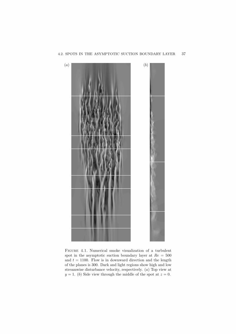
4.2. SPOTS IN THE ASYMPTOTIC SUCTION BOUNDARY LAYER 37

(a) (b)

Figure 4.1. Numerical smoke visualization of a turbulentspot in the asymptotic suction boundary layer at Re = 500and t = 1100. Flow is in downward direction and the lengthof the planes is 300. Dark and light regions show high and lowstreamwise disturbance velocity, respectively. (a) Top view aty = 1. (b) Side view through the middle of the spot at z = 0.

38 4. TURBULENCE

(a) (b)

Figure 4.2. Numerical smoke visualization of a turbulentspot in the asymptotic suction boundary layer at Re = 800and t = 900. Flow is in downward direction and the length ofthe planes is 300. Dark and light regions show high and lowstreamwise disturbance velocity, respectively. (a) Top view aty = 1. (b) Side view through the middle of the spot at z = 0.

4.3. TURBULENCE STATISTICS OF THE Blasius WALL JET 39

(a)

(b)

Figure 4.3. Numerical smoke visualization of a turbulentspot in the asymptotic suction boundary layer at Re = 1200and t = 500. Flow is from left to right and the length ofthe planes is 200. Dark and light regions show high and lowstreamwise disturbance velocity, respectively. (a) Top view aty = 1. (b) Side view through the middle of the spot at z = 0.

The fully developed turbulent spot grows linearly both in length and width.The leading edge propagates at about 85-90% of the free-stream velocity whilethe trailing edge velocity decreases from slightly bellow 70% for Re = 500to slightly bellow 50% for Re = 1200. The half-width angle increases withincreasing Reynolds number from about 2◦ for Re = 500 to about 4◦ for Re =1200. However, it seems to level off to a constant value at high Reynoldsnumbers. At the time of writing this thesis, an ongoing experiment of turbulentspots in the asymptotic suction boundary layer at Re = 500 is performed inthe MTL wind-tunnel at KTH Mechanics in Stockholm by Jens Fransson. Hispreliminary results indicate slightly larger spreading rates.

To summarize, the turbulent spot in the asymptotic suction boundary layerbears many similarities to spots in other flows. Its shape and spreading rates arereminiscent of the turbulent spot in boundary layers subjected to a favorablepressure gradient. In common with spots in plane Couette flow and planePoiseuille flow, the spreading rates are dependent of the Reynolds number.

4.3. Turbulence statistics of the Blasius wall jet

In the sixth paper, the early turbulent evolution of the Blasius wall jet is stud-ied. The investigation is an extension of the simulation presented in paper 3.The same forcing with two-dimensional waves and streamwise elongated streaksis done to trigger a natural transition mechanism. However, a four times largercomputational domain is used, allowing the turbulent region of the wall jet todevelop for a longer distance downstream. Statistics of mean flow and turbulentstresses are sampled for 2200 time units, corresponding to five months of non-stop simulations. The averaged data is then scaled with appropriate scalingsfor the inner boundary layer and the outer shear layer to identify self-similarbehavior.

40 4. TURBULENCE

0 0.5 10

0.5

1

1.5

2

0.1 1 10 1000

2

4

6

8

10

12

14

16(a) (b)

y

y1/2

U/Um

U+

y+

U+ = y+

Figure 4.4. Mean streamwise velocity at x = 170 (solid line),200 (dashed line), 250 (dashed-dotted line) and 300 (dottedline). (a) Outer scaling is used. (b) Inner scaling is used.

For the outer scaling, velocities are scaled with the local maximum veloc-ity of the wall jet Um and lengths are scaled with the half-width y

1/2, which is

the distance from the wall where the velocity in the outer region reaches halfthe local maximum velocity. The streamwise mean velocity scaled with outerscaling is shown in figure 4.4(a). The profiles between x = 200 and 300 collapsereasonably well up to y/y

1/2= 1. Further away from the wall, the profiles devi-

ate from each other owing to a secondary flow. This secondary flow originatesfrom a start-up vortex that slowly convects downstream and then remains inthe ambient flow in front of the fringe region, which seems to act like a wall onsuch large structures. External flows exist for wall jets in experimental facilitiesas well, but as the computational box is not as large as the surrounding spacein an experiment, the problem is more prominent. It is possible to avoid thevortex by specifying the entrainment velocity at the upper boundary as wasdone by Dejoan & Leschziner (2005), who used a boundary condition based onthe laminar free plane jet. However, it is chosen not to constrain the turbulentwall jet by prescribing an entrainment velocity based on laminar theory.

When using the inner scaling, velocities are scaled with the friction ve-locity uτ =

√

ν|∂U(y = 0)/∂y| and lengths are scaled with the wall thicknessη = ν/uτ . Quantities scaled with the inner scaling are conventionally denotedwith a plus (e.g. y+ = y/η and uv+ = u′v′/u2

τ). Using this notation, the half-width corresponds to about 300 plus units, a value that increases with Reynoldsnumber. Figure 4.4(b) shows the near-wall region of the streamwise mean ve-locity scaled with inner scaling. Within the viscous sublayer, the profiles followa linear law U+ = y+, shown as the gray line, up to about y+ = 4. Further

4.3. TURBULENCE STATISTICS OF THE Blasius WALL JET 41

0.1 1 10 1000

1

2

3

0.1 1 10 1000

0.5

1

1.5

2

0.1 1 10 100−1

0

1

2

0.1 1 10 1000

2

4

6

8

(a) (b)

(c) (d)

u+ v+

uv+ k+

y+ y+

y+ y+

Figure 4.5. Profiles of (a) rms of u′, (b) rms of v′, (c) Rey-nolds shear stress and (d) turbulence kinetic energy. Lines asin figure 4.4.

away from the wall, the profiles start to deviate from the linear behavior, earlierthan for a turbulent boundary layer that typically start to deviate for valuesy+ ≥ 8. Up to about y+ = 20, the profiles at x = 250 and 300 collapse well.

Components of the Reynolds stress and the turbulent kinetic energy scaledwith inner scaling are shown in figure 4.5 for the same streamwise positions asin figure 4.4. The profiles collapse reasonably well for the streamwise positionsx = 200 to 300 indicating that the flow has started to exhibit a self-similarbehavior. It can be noted that the collapse provided with inner scaling is muchbetter than with outer scaling. The profile at the position x = 170 is, however,still close to the transitional region and deviates from the other profiles. Thegeneral shape of the profiles agree well with previous studies (e.g. Erikssonet al. 1998; Dejoan & Leschziner 2005). However, downstream of the positionx = 300, the vortex present in the end of the computational domain causes theflow to depart from the self-similar behavior and profiles from this region aretherefore not taken into account.

CHAPTER 5

Conclusions

The work presented in this thesis is motivated by the need of an increasedfundamental understanding of the physics of wall-bounded flows. Investiga-tions of the stability, transition mechanism and early turbulent evolution ofwall-bounded flows have therefore been carried out. Three base flows havebeen considered, the Falkner–Skan boundary layer subjected to favorable, zeroand adverse pressure gradients, boundary layers subjected to wall suction andthe Blasius wall jet. The stability was investigated by means of linear sta-bility equations valid both for the exponential and algebraic growth scenario.An adjoint-based optimization technique was used to optimize the algebraicgrowth of streaks. The exponential growth of waves was maximized in thesense that the envelope of the most amplified eigenmode has been calculated.The transition mechanism and turbulence were studied by direct numericalsimulations.

In the first paper, the stability of the Falkner–Skan boundary layer sub-jected to favorable, zero and adverse pressure gradients is considered. Theoptimization of the algebraic growth was carried out over the initial stream-wise location as well as the spanwise wavenumber and the angular frequency.It it found that the initial streamwise location, where the disturbance is in-troduced in the boundary layer, has a significant impact on the growth. Theoptimal location moves downstream with decreased pressure gradient of thebase flow. In both the algebraic and exponential growth scenarios, the growthis found to increase with increased pressure gradient, although the effect ismuch more pronounced for the exponential growth. Furthermore, a unifiedtransition prediction method incorporating the influences of pressure gradientand free-stream turbulence is suggested.

In the second paper, the algebraic growth of streaks in boundary layerssubjected to wall suction is considered. It is found that the spatial analysis giveslarger optimal growth in the asymptotic suction boundary layer than temporaltheory. Furthermore, it is found that the optimal growth is larger for thesemi suction boundary layer, where the suction begins a distance downstreamof the leading edge, than for the asymptotic suction boundary layer. Theupstream part of the boundary layer without suction is responsible for thisincrease of the growth as well as the decrease of the corresponding wavenumber.However, when the streamwise interval for which the optimization is carriedout is prolonged, the differences reduce.

42

5. CONCLUSIONS 43

In the third paper, the Blasius wall jet, which was matched to the measuredflow in an experimental wall-jet facility, is considered. Linear stability analysiswith respect to the growth of two-dimensional waves and streamwise streakswas performed and compared to the experiments. The flow reveals a high in-stability to two-dimensional waves and non-modal streaks. Furthermore, thenonlinear interaction of introduced waves and streaks and the flow structurespreceding the flow breakdown were investigated by means of direct numericalsimulations. It is demonstrated that the streaks play an important role in thebreakdown process, where their growth is transformed from algebraic to expo-nential as they become part of the secondary instability of the two-dimensionalwaves. The role of subharmonic waves and pairing of vortex rollers was alsoinvestigated. However, in the presence of streaks, pairing is suppressed andbreakdown to turbulence is enhanced.

In the fourth paper, energy thresholds for transition to turbulence in theasymptotic suction boundary layer are considered. The development and break-down of periodic disturbances were studied with direct numerical simulations.Transition triggered by streamwise vortices, oblique waves and random noisewere investigated. It is found that the lowest energy threshold is providedby the oblique wave scenario for the considered Reynolds numbers (Re). Thethreshold energy is found to scale like Re−2.6 for oblique transition and likeRe−2.1 for transition initiated by streamwise vortices and random noise. Thisindicates that oblique transition has the lowest energy threshold also for largerReynolds numbers.

In the fifth paper, thresholds for transition of localized disturbances, theirbreakdown to turbulence and the development of turbulent spots in the as-ymptotic suction boundary layer are considered. The localized disturbancewas introduced in the initial base flow and studied using direct numerical sim-ulations. It is found that the threshold amplitude, defined as the maximumwall-normal disturbance velocity, scales like Re−1.5 for 500 ≤ Re ≤ 1200. ForRe ≤ 367, the localized disturbance decays after the initial transient growth.The turbulent spot is found to take a bullet-shaped form with a rounded leadingedge and a straight trailing edge. Long streaks extend upstream evolving fromthe disturbed flow in an overhang region. It is found that the spot becomesmore distinct and increases its spreading rate for higher Reynolds number.

In the sixth paper, the early turbulent evolution of the Blasius wall jet isconsidered. The direct numerical simulation is an extension of the work pre-sented in paper 3 but a larger computational domain was used. The averageddata from turbulence statistics was scaled in both inner and outer scaling inorder to identify self-similar behavior. Despite the low Reynolds number andthe short computational domain, in comparison to available experiments, itwas found that the turbulent flow exhibits a reasonable self-similar behavior,which is most pronounced with inner scaling in the near-wall region.

Acknowledgment

First of all, I would like to thank my supervisor, Professor Dan Henningson, forgiving me the opportunity to work as his student and to develop my knowledgewithin the subject of fluid dynamics. He is always very helpful and brings joyinto good as well as bad days at the office. In particular, I value his professionalway to work and his personal way to be a friend.

I want to thank Doctor Jan Pralits, my previous colleague and office mate,for all the time he spent to help me to get started with the project. He wasalways very helpful and encouraging when ever I needed help.

I also want to thank Doctor Mattias Chevalier for the help with variousmodifications of the spectral code and Doctor Luca Brandt for the guidancewith the direct numerical simulations. Furthermore, I would like to thankAssociate Professor Ardeshir Hanifi who could sit for hours to help me withthe stability codes.

I would like to thank my co-authors Valery Chernoray and Lennart Lofdahlat Chalmers, Niklas Davidsson at Lulea University, Martin Bystrom, AstridHerbst and Dan Henningson at KTH Mechanics for nice collaborations.

Many thanks to my colleagues at KTH Mechanics for providing a verynice atmosphere at the Department. In particular I would like to thank AstridHerbst, Carl-Gustav Unckel, Dan Henningson, Erik Stalberg, Espen Akervik,Fredrik Lundell, Jan Pralits, Jens Fransson, Jerome Hœpffner, Luca Brandt,Markus Hogberg, Martin Bystrom, Martin Skote, Mattias Chevalier and I alsowant to thank the Department for providing the gym card and the opportunityto play indoor bandy.

This work has been funded by the Swedish Energy Agency (Energimyn-digheten). The large direct numerical simulations were performed at the Centerfor Parallel Computers at KTH.

Finally, I want to thank my mother Doris and my father Robert for all thesupport that made this possible, my grandmother Gertrud, my grandfatherHarry and all my friends. Special thanks are given to my lovely girlfriendLinda for all her love and support.

44

Bibliography

Abu-Ghannam, B. J. & Shaw, R. 1980 Natural transition of boundary layers - theeffects of turbulence, pressure gradient, and flow history. J. Mech. Eng. Sci. 22,213–228.

Andersson, P., Berggren, M. & Henningson, D. S. 1999 Optimal disturbancesand bypass transition in boundary layers. Phys. Fluids 11, 134–150.

Bajura, R. A. & Catalano, M. R. 1975 Transition in a two-dimensional plane walljet. J. Fluid Mech. 70, 773–799.

Bajura, R. A. & Szewczyk, A. A. 1970 Experimental investigation of a laminartwo-dimensional plane wall jet. Phys. Fluids 13, 1653–1664.

Bech, K. H., Henningson, D. S. & Henkes, R. A. W. M. 1998 Linear and nonlin-ear development of localized disturbances in zero and adverse pressure gradientboundary-layers. Phys. Fluids 10, 1405–1418.

Bernal, L. P. & Roshko, A. 1986 Streamwise vortex structure in plane mixinglayers. J. Fluid Mech. 170, 499–525.

Bertolotti, F. P., Herbert, T. & Spalart, P. R. 1992 Linear and nonlinearstability of the Blasius boundary layer. J. Fluid Mech. 242, 441–474.

Boiko, A. V., Westin, K. J. A., Klingmann, B. G. B., Kozlov, V. V. &

Alfredsson, P. H. 1994 Experiments in a boundary layer subjected to freestream turbulence. Part 2. The role of TS-waves in the transition process. J.Fluid Mech. 281, 219–245.

Breuer, K. S. & Haritonidis, J. H. 1990 The evolution of a localized disturbancein a laminar boundary layer. Part 1. Weak disturbances. J. Fluid Mech. 220,569–594.

Breuer, K. S. & Landahl, M. T. 1990 The evolution of a localized disturbancein a laminar boundary layer. Part 2. Strong disturbances. J. Fluid Mech. 220,595–621.

Chun, D. H. & Schwarz, W. H. 1967 Stability of the plane incompressible viscouswall jet subjected to small disturbances. Phys. Fluids 10, 911–915.

Corbett, P. & Bottaro, A. 2000 Optimal perturbations for boundary layers sub-ject to stream-wise pressure gradient. Phys. Fluids 12, 120–130.

Dejoan, A. & Leschziner, M. A. 2005 Large eddy simulation of a plane turbulentwall jet. Phys. Fluids 17, 025102.

van Driest, E. R. & Blumer, C. B. 1963 Boundary layer transition: Freestreamturbulence and pressure gradient effects. AIAA J. 1, 1303–1306.

45

46 BIBLIOGRAPHY

Dryden, H. L. 1959 Transition from laminar to turbulent flow. In Turbulent flowsand heat transfer (ed. C. C. Lin), pp. 1–74. Princeton University Press.

Ellingsen, T. & Palm, E. 1975 Stability of linear flow. Phys. Fluids 18, 487–488.

Eriksson, J. G., Karlsson, R. I. & Persson, J. 1998 An experimental study of atwo-dimensional plane turbulent wall-jet. Exps. Fluids 25, 50–60.

Fjørtoft, R. 1950 Application of integral theorems in deriving criteria for instabilityfor laminar flows and for the baroclinic circular vortex. Geofys. Publ., Oslo 17,1–52.

Floryan, J. M. & Saric, W. S. 1979 Stability of Gortler vortices in boundarylayers. AIAA J. 20, 316–324.

Fransson, J. H. M. & Alfredsson, P. H. 2003 On the disturbance growth in anasymptotic suction boundary layer. J. Fluid Mech. 482, 51–90.

Fransson, J. H. M. & Corbett, P. 2003 Optimal linear growth in the asymptoticsuction boundary layer. Eur. J. Mech. B/Fluids 22, 259–270.

Gogineni, S. & Shih, C. 1997 Experimental investigation of the unsteady structureof a transitional plane wall jet. Exp. Fluids 23, 121–129.

Hall, P. 1983 The linear development of Gortler vortices in growing boundary layers.J. Fluid Mech. 130, 41–58.

Hanifi, A. 1995 Local and non-local stability analysis and transition prediction ofcompressible boundary layer flows. PhD thesis, Royal Institute of Technology,Stockholm, Sweden.

Hein, S., Stolte, A. & Dallmann, U. C. 1999 Identification and analysis of nonlin-ear transition scenarios using NOLOT/PSE. Z. Angew. Math. Mech. 79, S109–S112.

Henningson, D. S. 1996 Comment on ”Transition in shear flows. Nonlinear normal-ity versus non-normal linearity” [Phys. Fluids 7, 3060 (1995)]. Phys. Fluids 8,2257–2258.

Henningson, D. S., Lundbladh, A. & Johansson, A. V. 1993 A mechanism forbypass transition from localized disturbances in wall-bounded shear flows. J.Fluid Mech. 250, 169–238.

Hocking, L. M. 1975 Non-linear instability of the asymptotic suction velocity profile.Quart. J. Mech. Appl. Math. 28, 341–353.

van Ingen, J. L. 1956 Suggested semi-empirical method for the calculation of theboundary layer transition region. Tech. Rep. UTH-74. Dep. of Aero. Eng., Uni-versity of Technology, Delft.

Klebanoff, P. S. 1971 Effect of freestream turbulence on the laminar boundarylayer. Bull. Am. Phys. Soc. 10, 1323.

Kosorygin, V. S. & Polyakov, N. P. 1990 Laminar boundary layers in turbulentflows. In Laminar-Turbulent Transition (eds. D. Arnal & R. Michel), pp. 573–578. Springer.

Landahl, M. T. 1980 A note on an algebraic instability of inviscid parallel shearflows. J. Fluid Mech. 98, 243–251.

Lasheras, J. C., Cho, J. S. & Maxworthy, T. 1986 On the origin and evolutionof streamwise vortical structures in a plane, free shear layer. J. Fluid Mech. 172,231–258.

Lorenz, E. N. 1963 The predictability of hydrodynamic flow. Trans. NY Acad. Sci.25, 409–432.

BIBLIOGRAPHY 47

Lundbladh, A., Berlin, S., Skote, M., Hildings, C., Choi, J., Kim, J. &

Henningson, D. S. 1999 An efficient spectral method for simulation of incom-pressible flow over a flat plate. Tech. Rep. KTH, Department of Mechanics,Stockholm.

Mack, L. M. 1977 Transition prediction and linear stability theory. In AGARD-CP-224 , pp. 1–1 to 1–22. NATO, Paris.

Mathew, J. & Das, A. 2000 Direct numerical simulations of spots. Current Science79, 816–820.

Matsubara, M. & Alfredsson, P. H. 2001 Disturbance growth in boundary layerssubjected to free-stream turbulence. J. Fluid Mech. 430, 149–168.

Mele, P., Morganti, M., Scibilia, M. F. & Lasek, A. 1986 Behavior of wall jetin laminar-to-turbulent transition. AIAA J. 24, 938–939.

Metcalfe, R. W., Orszag, S. A., Brachet, M. E., Menon, S. & Riley, J. J.

1987 Secondary instability of a temporally growing mixing layer. J. Fluid Mech.184, 207–243.

Nordstrom, J., Nordin, N. & Henningson, D. S. 1999 The fringe region techniqueand the Fourier method used in the direct numerical simulation of spatiallyevolving viscous flows. SIAM J. Sci. Comput. 20, 1365–1393.

Orr, W. M. F. 1907 The stability or instability of the steady motions of a perfectliquid and of a viscous liquid. Part I: A perfect liquid. Part II: A viscous liquid.Proc. R. Irish Acad. A 27, 9–138.

Pretsch, J. 1941 Die stabilitat einer ebenen laminarstromung bei druckgefalle unddruckanstieg. Jb. dt. Luftfahrtforschung I pp. 54–71.

Reyleigh, L. 1880 On the stability of certain fluid motions. Proc. Math. Soc. Lond.11, 57–70.

Reynolds, O. 1883 An experimental investigation of the circumstances which deter-mine whether the motion of water shall be direct or sinuous, and of the law ofresistance in parallel channels. Phil. Trans. Royal Soc. 174, 935–982.

Riley, J. J. & Gad-el-Hak, M. 1985 The dynamics of turbulent spots. In Frontiesin Fluid Mechanics (eds. S. H. Davis & J. L. Lumley), pp. 123–155. Springer.

Roach, P. E. & Brierley, D. H. 1992 The influence of a turbulent free-streamon zero pressure gradient transitional boundary layer development. I. Test casesT3A and T3B. In Numerical Simulation of Unsteady Flows and Transition toTurbulence (eds. O. Pironneau, W. Rodi, I. L. Ryhming, A. M. Savill & T. V.Truong), pp. 303–316. Cambridge University Press.

Schlichting, H. 1933 Berechnung der anfachung kleiner storungen bei der platten-stromung. ZAMM 13, 171–174.

Schoppa, W., Hussain, F. & Metcalfe, R. W. 1995 A new mechanism of small-scale transition in a plane mixing layer: core dynamics of spanwise vortices. J.Fluid Mech. 298, 23–80.

Schubauer, G. B. & Skramstad, H. F. 1947 Laminar boundary layer oscillationsand stability of laminar flow. J. Aero. Sci. 14, 69–78.

Smith, A. M. & Gamberoni, N. 1956 Transition, pressure gradient and stabilitytheory. Tech. Rep. ES 26388. Douglas Aircraft Co., EL Segundo, Calif.

Sommerfeld, A. 1908 Ein beitrag zur hydrodynamischen erklarung der turbulentenflussigkeitbewegungen. In Atti del 4 Congr. Internat. dei Mat. III , pp. 116–124.Roma.

48 BIBLIOGRAPHY

Squire, H. B. 1933 On the stability for three-dimensional disturbances of viscousfluid flow between parallel walls. Proc. Roy. Soc. Lond. Ser. A 142, 621–628.

Suder, K. L., O’Brien, J. E. & Reshotko, E. 1988 Experimental study of bypasstransition in a boundary layer. NASA TM 100913.

Tollmien, W. 1929 Uber die entstehung der turbulenz. Nachr. Ges. Wiss Gottingen,21–44, (English translation NACA TM 609, 1931).

Wernz, S. & Fasel, H. F. 1996 Numerical investigation of unsteady phenomena inwall jets. AIAA Paper 96-0079.

Wernz, S. & Fasel, H. F. 1997 Numerical investigation of forced transitional walljets. AIAA Paper 97-2022.

Westin, K. J. A., Boiko, A. V., Klingmann, B. G. B., Kozlov, V. V. &

Alfredsson, P. H. 1994 Experiments in a boundary layer subjected to freestream turbulence. Part 1. Boundary layer structure and receptivity. J. FluidMech. 281, 193–218.

Yang, Z. Y. & Voke, P. R. 1991 Numerical simulation of transition under turbu-lence. Tech. Rep. ME-FD/91.01. Dept. Mech. Eng. University of Surrey.

Numerical studies of transition in wall-bounded ﬂows Ori...

Documents

Transcript of Numerical studies of transition in wall-bounded ﬂows Ori...