NUMERICAL SOLUTION OF THE KOHN-SHAM …NUMERICAL SOLUTION OF THE KOHN-SHAM EQUATION BY FINITE...

NUMERICAL SOLUTION OF THE KOHN-SHAM EQUATION BY

FINITE ELEMENT METHODS WITH AN ADAPTIVE MESH

REDISTRIBUTION TECHNIQUE

GANG BAO†‡ , GUANGHUI HU† , AND DI LIU†

Abstract.

A finite element method with an adaptive mesh redistribution technique is presented for solvingthe Kohn-Sham equation. The mesh redistribution strategy is based on the harmonic mapping,and the movement of grid points is partially controlled by the monitor function that depends onthe gradient of the electron density. Compared with fixed meshes, both efficiency and accuracy ofthe solution are improved significantly. Effectiveness and robustness of the solver are illustrated bynumerical experiments.

Key words. adaptive mesh redistribution, harmonic map, finite element method, Kohn-Shamequation, density functional theory

AMS subject classifications. 65N30, 65N55, 81Q05

1. Introduction. The Schrodinger equation is fundamental for describing thequantum mechanical electronic structure of matter, since it dose not require anyempirical input[30]. The time-independent Schrodinger equation takes the followingform

HΨ = EΨ,(1.1)

where H is the Hamiltonian operator, and E and Ψ represent the energy eigenvalueand eigenstate (wave-function), respectively. Unfortunately, it is too expensive tosolve Eq. (1.1) directly because of the high dimensionality. In fact, Ψ here is amulti-variable function which depends on the position of every electron in the system.To this day, it is impossible to simulate a small molecule which consists of only adozen of electrons by solving (1.1) directly. Therefore it is imperative to reduce thecomputational cost of the solution of the Schrodinger equation.

Various methods have been proposed to simplify the numerical simulation of solu-tions of the Schrodinger equation. The density functional theory (DFT) is an impor-tant one among them. In 1964, Hohenberg and Kohn [16] discovered the one-to-onecorrespondence between the ground state electron density n(~x) and the external po-tential. According to their theorem, n(~x) can be treated as the fundamental unknownin a many-electron system. Because n(~x) is a function which only depends on threespatial coordinates, numerical simulations of large molecules or even solids becomepossible.

Inspired by Hohenberg and Kohn’s theoretical results, Kohn and Sham [19] pre-sented an implementation of DFT. The idea is to replace the physical system of inter-acting electrons with a fictitious system (the Kohn-Sham system) of non-interactingelectrons. These two systems have the same ground state electron density. In theKohn-Sham system, an electron is supposed to move in an effective potential, consistsof three terms: the external potential which is usually generated by the attractionbetween the electron and the nucleus, the Hartree potential which describes the re-pulsion between electron and electron, and the exchange-correlation potential which

†Department of Mathematics, Michigan State University, East Lansing, MI 48824, USA([email protected], [email protected], [email protected])

‡Department of Mathematics, Zhejiang University, Hangzhou 310027, China

1

2 MESH REDISTRIBUTION TECHNIQUE FOR THE KOHN-SHAM EQUATION

is caused by certain non-classical Coulomb interactions. Among these terms, theexchange-correlation potential can not be known analytically, which means that weneed some approximate methods to mimic it. In [19], Kohn and Sham introduced alocal density approximation (LDA) for the exchange-correlation potential, which isalso a key contribution of their work [29]. Since then, many other approximations havebeen proposed such as the generalized gradient approximation (GGA) [25, 27], themeta-generalized gradient approximation (meta-GGA) [6, 7]. By numerically solvingthe Kohn-Sham equation, we can determine the ground state electron density of theoriginally physical system, and therefore other interested quantities.

There are many numerical methods for solving the Kohn-Sham equation. Onepopular way is to use a plane-wave basis [21], which is based on the plane-wave ex-pansion of the Kohn-Sham orbitals. The plane-wave basis set is orthonormal andthe convergence of the calculations increases systematically with the number of theplane-waves. Many software packages have emerged, such as ABINIT [3], VASP [2],and KSSOLV[36] based on the plane-wave basis method. However, there are somedrawbacks for this method. For instances, the plane-wave basis method is not suit-able for the simulation of the non-periodic system. Because the basis is non-local inreal space, it results in dense matrices, which is ill-suited for iterative schemes. Toovercome these disadvantages, real-space discretization methods such as finite differ-ence methods, finite element methods and the wavelet methods have been proposedto solve the Kohn-Sham equation. All these real-space methods can adopt differentboundary conditions flexibly, and the resulting matrices are sparse which can be savedor operated much more efficiently. For an overview of all these numerical schemes andcorresponding software, we refer to [29, 32] and references therein.

We focus on the finite element methods in this paper, which have been widelyused in many different fields such as structural mechanics, fluid dynamics, electromag-netics. Early works [10, 30, 37] have been done for the applications of finite elementmethods on solving the Kohn-Sham equation. One advantage of these methods isthe flexibility. Different boundary conditions such as Dirichlet boundary condition,periodic boundary condition can be implemented by the finite element methods in astraightforward way. Compared with the finite difference methods, it is much moresuitable to discretize the governing equation on the complicated domain by using thefinite element methods. Furthermore, since the finite element methods are based onthe variational principle, the ground state energy can be approximated monotonicallyby refining the mesh or by enriching the order of the local approximation polynomi-als. In the calculations of the finite element methods, the physical domain is dividedinto small elements. For example, the tetrahedral element in this paper. It is still achallenging task to generate a high-quality tetrahedral mesh. In this paper, we getthe tetrahedral mesh by a software named GMSH[1], which is an open-source softwareand published under GPL license. For the Kohn-Sham equation, especially for theall-electron calculations, the external potential is singular in the vicinity of the nu-cleus. Therefore, there is no hope to get a high-quality approximation of the solutionsif this singularity is not resolved effectively. On the other hand, the problem in thispaper is non-periodic, which means that the physical domain should be sufficientlylarge to reduce the truncation error from the boundary.

Based on above discussion, using the radial mesh seems to be a good choice.The radial mesh has small mesh size in the vicinity of each nucleus, and large onein the region away from nucleus. For this configuration of mesh, a large amount ofgrid points locate at the vicinity of nucleus, which can help to resolve the singular

GANG BAO, GUANGHUI HU AND DI LIU 3

external potential. For the region away from nucleus, since there is almost no variationfor the potentials, wave-functions and electron density, just a few of grid points areneeded. Based on this idea, two well-designed non-uniform meshes are given in [30,22] respectively, and excellent numerical results are demonstrated there. Besidesgenerating well-designed mesh beforehand, the adaptive technique is another way toimprove the mesh quality.

There exist three classical adaptive methods: the h-adaptive methods which lo-cally refine and coarsen the mesh, the r-adaptive methods which redistribute the gridpoints while keeping the number of mesh grids unchanged, and the p-adaptive meth-ods which locally enrich the order of the approximate polynomial. The r-adaptivemethod is also known as the moving mesh method. To solve the Kohn-Sham equationwith the h-adaptive methods, there are already some results, see [37, 10]. Interestingdiscussions may be found on the application of the hp-adaptive methods to solvingthe Kohn-Sham equation in [32]. In particular, an interesting observation was madein [32] “The question of the feasibility of molecular dynamics with an unstructured

nonuniform FE-mesh is often raised. The FE-community provides the following sug-

gestion, based on experience in other fields: each atom is attached to the mesh, and

the mesh is considered to be made of ‘rubber’. As the atom moves, the mesh moves

along...”. Based on our numerical experience, r-adaptive methods can partially satisfythe above requirements. A motivation of our current work is to propose a frameworkfor solving the Kohn-Sham equation by using the r-adaptive methods. For the earlywork on this topic, we refer to [33] and references therein.

In this paper, we present a finite element solver with a r-adaptive technique tosimulate the Kohn-Sham equation with tetrahedral meshes. The solver consists of twomain iterations. The first one is a SCF iteration to generate a self-consistent electrondensity on the current mesh, while the second iteration is adopted to adaptively opti-mize the distribution of mesh grids in terms of the electron density. The Kohn-Shamequation is discretized by the standard finite element method. The Hartree poten-tial is obtained by solving the Poisson equation with an algebraic multi-grid (AMG)method. The exchange-correlation potential is approximated by the local density ap-proximation (LDA). On the boundary of the domain, the zero Dirichlet boundarycondition is adopted for the wave-function. However, it is not the case for solvingthe Poisson equation. For the boundary condition of the Poisson equation, becausethe Hartree potential decays linearly, the boundary value is supplied by the multipoleexpansion. The NSRQMCG method [15] is the solver for the final generalized eigen-value problem. To improve the convergence of SCF iteration, a linear mixing schemeis adopted to update the electron density. After the self-consistent electron density isobtained, an adaptive technique for the redistribution of the mesh grids is introducedfor improving the mesh quality. The redistribution technique we used in the paper isoriginally presented by Li. et al. in [23, 24], and has been widely applied in differentapplication fields. A review of the method may be found in [31]. Theoretically, thistechnique is based on the harmonic mapping, which maps a uniform mesh in a logicaldomain to a non-uniform mesh in a physical domain. The map is controlled partiallyby a so-called monitor function.

Based on our numerical experience, the monitor function is always given accord-ing to certain posteriori error estimates of numerical solutions or information fromthe physical solution itself. In the domain for solving the Kohn-Sham equation, com-pared with the distant regions from the atom, the regions around the atomic nucleiand between atoms of chemical bonds are more important[37]. More grid points are


expected to be arranged in these regions. Therefore, the monitor function is givenbased on the gradient of the electron density, and it can be observed from the resultsthat those important regions are resolved successfully with this monitor function.

To guarantee the numerical accuracy, it is important to keep the smoothness andorthogonality of mesh grids after the mesh movement. In the r-adaptive methods,these requirements are satisfied by smoothing the monitor function. As mentionedbefore, the physical domain should be sufficiently large, while the interested region isjust the vicinity of each nucleus. Hence the smoothness method proposed in [23, 24]is no longer adequate. By employing a smoothness strategy similar to [35, 34, 17]based on a diffusive mechanism of the monitor function, the mesh quality may besignificantly improved as shown in the numerical experiments.

The outline of this paper is as follows. In the next section, the DFT and the Kohn-Sham equation are introduced. In Section 3, the finite element discretization of theKohn-Sham equation is described. A mesh redistribution technique is also introducedin Section 4. In Section 5, some details of numerical techniques are discussed on ouralgorithm. Numerical simulations are demonstrated in Section 6, which illustrate thereliability and the effectiveness of our method. Finally, the paper is concluded withsome general remarks as well as discussions on future directions in Section 7.

2. The Kohn-Sham Equation. In [19], Kohn and Sham presented the fol-lowing self-consistent equation to reach the minimization of the total energy of amany-electron system (we use the atomic units e2 = h = m = 1 hereafter)

(

T + veff (~x))

ψi(~x) = εiψi(~x),(2.1)

where T = − 1

2∇2 denotes the kinetic energy, veff (~x) is the effective potential with

the following expression

veff (~x) = vext(~x) + vHartree(~x) + vxc(~x).(2.2)

For a closed system of M nuclei and N electrons, the external potential

vext(~x) = −M∑

i

Zi

|~x− ~xi|,(2.3)

describes the attraction between the nucleus and electron. Here Zi is the i-th nucleuscharge, and ~xi is the position of the i-th nucleus. The Hartree potential vHartree isthe Coulomb interaction of electrons

vHartree(~x) =

∫

n(~x′)

|~x− ~x′|d~x′.(2.4)

In the simulation, direct evaluating the above integral will result in O(N2) operations,which is very time-consuming. A popular way to address vHartree is to solve thefollowing Poisson equation

−∇2vHartree(~x) = 4πn(~x).(2.5)

with a proper Dirichlet boundary condition.The last term in (2.2) is the exchange-correlation potential vxc(~x). This term is

caused by the Pauli exclusion principle and other non-classical Coulomb interactions.


Unfortunately, the analytical expression of the exchange-correlation potential for ageneral system is unknown. Thus this term needs to be approximated. The mostpopular way is to use the local density approximation (LDA) originally proposed byKohn and Sham in [19]. The exchange-correlation energy ELDA

xc (n) is given as

ELDAxc (n) =

∫

ǫxc(n)n(~x)d~x.(2.6)

where ǫxc(n) stands for the exchange-correlation energy per unit volume of the ho-mogeneous electron gas of the density n. Then vxc can be addressed as

vxc(~x) =δExc

δn.(2.7)

The exchange-correlation energy Exc can be separated as two parts Exc = Ex+Ec.We adopt the expression of the exchange energy Ex proposed in [19]

ELDAx (n) = −3

4(3

π)1/3

∫

n(~x)4/3d~x.(2.8)

Then vx = −(3n(~x)/π)1/3. The approximation of Ec is much more complicated thanthat of Ex. Even in the free electron gas, we only know the expressions of Ec of thehigh-density limit and the low-density limit. In the simulation, the parametrizationof Perdew and Wang [28] fitted to accurate Monte Carlo simulations carried out byCeperley and Alder [11] is adopted.

From (2.1), we can see that the wave-function ψi(~x) depends on the effectivepotential veff (~x), while the electron density n(~x) which has the following relationshipwith ψi(~x)

n(~x) =

occ∑

i

|ψi(~x)|2,(2.9)

determines the effective potential veff at the meantime. That means the equation(2.1) is non-linear, and we need a self-consistent field (SCF) method to solve it.

Finally, we present the formula to calculate the ground state energy of the physicalsystem from the solution of the Kohn-Sham equation:

E =

occ∑

i

εi −∫ (

1

2vHartree + vxc

)

n(~x)d~x+ Exc.(2.10)

Note that for the simulations of a molecule which contains several nuclei, the totalenergy should be added to a repulsive Coulomb term that accounts for the interactionsbetween the nuclei

Enn =∑

j,k

ZjZk

|~xj − ~xk|.

To solve (2.1), many numerical methods have been proposed. Here, we focus onthe finite element method for discretizing the governing equation because of its flexibil-ity on different geometries and boundary conditions. The finite element discretizationof (2.1) will be introduced in the next section.


3. Numerical Discretization. Assume that the physical domain is denoted byΩ ∈ R3, and Ω is divided into a set of tetrahedron T with Ti as its element and ~Xi

as its nodes. The piecewise linear finite element space Vh is built on T . Note that forthe linear finite element case, the interpolation points of the degrees of freedom (Dof)in each element locate on the vertexes of the tetrahedral element (3D case).

Based on the above assumptions, the wave-function ψ(~x) in (2.1) can be approx-imated as

ψh =

Nbasis∑

i

ψiφi,(3.1)

where Nbasis stands for the dimension of space Vh, and φi is the i-th basis functionand ψi is its coefficient, which is also the value of the wave-function itself on thecorresponding node.

For the finite element method, the variational approach is used to find out thecoefficients ψ = (ψ0, ψ1, ψ2, · · · , ψNbasis

)T , which leads to the following linear system

Aψ = εBψ.(3.2)

Here A and B are two matrices with the entries

Ai,j =1

2

∫

Ω

∇φi · ∇φjd~x+

∫

Ω

veffφiφjd~x,(3.3)

Bi,j =

∫

Ω

φiφjd~x,(3.4)

respectively.The equation (3.2) is actually a generalized eigenvalue problem with good prop-

erties, because the matrices A and B are both Hermitian, and the mass matrix B ispositive definite. There are many solvers in the literature to solve this kind of problemsuch as the Aronldi algorithm [5] (because A is symmetric, it is also known as theLanczos algorithm) which can be implemented by a software ARPack [4], and precon-ditioned conjugate gradient (PCG) method. In our algorithm, we use the NSRQMCGmethod [15] to search for the leftmost eigenpairs (εi, ψi), i = 1, 2, · · · of the equation(3.2).

To discretize the Poisson equation (2.5), we use the same finite element spacementioned above. The Hartree potential vHartree can be approximated as

vH,h =

Nbasis∑

i

vH,iφi,(3.5)

where vH,i is the coefficient of the i-th basis function φi. Let vH = (vH,0, vH,1, · · · , vH,Nbasis)T ,

then the final system can be read as

PvH = f,(3.6)

where P is the stiffness matrix with entry

Pi,j =

∫

Ω

∇φi∇φjd~x,(3.7)


and the right hand side f is a vector with entry

fi =

∫

Ω

4πn(~x)φid~x.(3.8)

Note that in the above integration, the evaluation of the electron density n(~x) on aquadrature point ~xq is given by

n(~xq) =

occ∑

i

Nbasis∑

j,k

φjψi,j(~xq)φkψi,k(~xq).

An efficient solver for the Poisson equation is important, because (3.6) needs tobe solved in each SCF iteration. In our algorithm, the algebraic multi-grid method isadopted. The implementation issues of this AMG solver will be discussed in Section5.

The electron density is obtained by a SCF iteration. That is, the wave-function ψis solved from (3.2), and then the electron density n(~x) is obtained from (2.9). Thenthe effective potential in (2.1) is evaluated in terms of the new n(~x). To end up theSCF iteration, the following criterion is used

‖nN+1(~x)− nN (~x)‖2 < tol,(3.9)

where nN (~x) and nN+1(~x) mean the electron densities obtained from two adjacentiterations, and tol is an user-defined tolerance.

Once the self-consistent electron density is obtained, an adaptive technique of themesh redistribution will be introduced to optimize the mesh quality, hence to improvethe accuracy of the numerical solution. In the next section, the mechanism of thistechnique is presented.

4. Mesh Redistribution. The mesh redistribution method in this paper isbased on the harmonic mapping. Since this technique was originally proposed in[23, 24], it has been widely applied to a variety of computational problems. We firstbriefly summarize the mechanism of this technique. Since we mainly focus on 3Dsimulations of the Kohn-Sham equation in this paper, the following definitions anddescription are all given in the 3D Euclidean space.

4.1. Harmonic maps. Suppose there are two compact Riemannian manifoldsΩ and Ωc with the metric tensors dij and rαβ in certain local coordinates ~x and ~ξ.

Define a map ~ξ = ~ξ(~x) between Ω and Ωc, then the energy of this map is given by

E(~ξ) =1

2

∫ √ddij

∂ξα

∂xi∂ξβ

∂xjd~x,(4.1)

where d = det(dij), (dij) = (dij)−1, and the standard summation convection is as-sumed. If the map ξ is an extremum of (4.1), ξ is called a harmonic map. This mapis the solution of the following Euler-Lagrange equation

∂

∂xi(Gij ∂ξ

k

∂xj) = 0,(4.2)

where the inverse of Gij =√ddij is called the monitor function.


The harmonic function ξ gives a continuous, one-to-one mapping from Ω to Ωc

with continuous inverse, which is differentiable and has a non-zero Jacobian [31]. Inpractice, we always use Ω as the physical domain, and Ωc as a reference domain,called the logical domain. With the help of harmonic maps, we can generate a non-uniform mesh in the physical domain Ω from an uniform mesh in the logical domainΩc by partially controlling the monitor function. To guarantee the existence and theuniqueness of the harmonic map, the Riemannian curvature of Ωc should be non-positive and its boundary should be convex[23]. In the simulations, we can directlyuse the physical domain (a cube) as the logical domain, and such selection obviouslysatisfies the above requirements.

4.2. Mesh redistribution using harmonic maps. Suppose the SCF itera-tion has been finished on current mesh, and the self-consistent electron density andwave-functions have been obtained. What we do in the next step is to reasonablyredistribute the mesh grids in terms of those self-consistent quantities, with the helpof the harmonic map.

In the practice, the harmonic map is reached by an iterative procedure. Assumethat an initial(fixed) mesh on the logical domain Ωc is given, the general frameworkof generation of the harmonic map can be described as the following.

Flow Chart of the Algorithm 1S. 1 obtain the difference between the current mesh which is obtained

from solving (4.3) and the initial mesh in the logical domain Ωc. Ifthe L∞ norm of the difference is smaller than a given tolerance, themesh redistribution is done, otherwise, go to next step;

S. 2 obtain the directions and the magnitudes of the movement of meshgrids in the physical domain Ω in terms of the difference given in S.

1, and then update the mesh in the physical domain;S. 3 update solutions on the updated mesh in the physical domain, then

go to S. 1.

In [23], the system which is used to generate the mesh in the logical domain in S.

1 is (4.2) together with a Dirichlet boundary condition. However, with this system,only the interior grids are redistributed, while the grid points on the boundary areunchanged. Under this situation, the redistribution of grids on the boundary of thephysical domain should be handled separately, such as using homogeneous Neumannboundary conditions, extrapolating the interior mesh points to the boundary, and re-locating the mesh points by solving a lower-dimensional moving-mesh PDE. However,all these strategies may affect the efficiency of the algorithm.

To redistribute the whole mesh grids in an uniform manner, Li et al. [24] proposedan optimization problem for the harmonic map in place of the boundary value problemin [23]. The optimization problem can be read as

min∑

k

∫

Ω

M∂ξk

∂xi∂ξk

∂xjd~x,

s. t. ξ|∂Ω = ξb ∈ K,

(4.3)

whereK = ξb ∈ C0(∂Ω)|ξb : ∂Ω → Ωc; ξb|Λiis a linear segment and strictly increasing

denotes a mapping set from ∂Ω to ∂Ωc. By solving the above optimization problem,


the mesh points including those on the boundary may be redistributed simultaneously.

In the following, details in each step of Algorithm 1 will be briefly demonstrated.Assume that the tetrahedral mesh in the physical domain Ω is denoted by T , with Tias its element, and Xi as its node. For the logical domain Ωc, we use Tc to denote thecorresponding tetrahedral mesh, and Ti,c and Ai as its element and node, respectively.

To obtain the initial mesh in the logical domain Ωc, we need to generate the initialmesh T ini

c in the logical domain Ωc by solving the following optimization problem

min∑

k

∫

Ω

∑

i

(∂ξk

∂xi)2d~x,

s. t. ξ|∂Ω = ξb ∈ K.

(4.4)

During the whole procedure, this initial mesh is only a reference, and unchanged.

In the first step of the Algorithm 1, the optimization problem (4.3) needs to besolved. Note that at the current stage, we only try to improve the mesh quality i.e., not the physical solution, the efficiency of the solver for (4.3) is more importantthan its accuracy. However, the linear system which is obtained from (4.3) is neitherHermitian nor positive definite. To resolve this difficulty, it was suggested in [24] thatthe system be decoupled into two smaller systems: one is for the grid points on theboundary, and the other one is for the interior grid points. Although there is also nogood property for the first system, it is much smaller than the original system, anda generalized minimal residual method (GMRES) or a biconjugate gradient (BiCG)method can be used to solve it. For the second one, a multi-grid method is adoptedto solve it because it has good properties (Hermitian and positive definite).

To further improve the efficiency of the solver for (4.3), Di et al. [13] proposeda new approach to speed up the implementation. This new approach is based onan algebraic multi-grid method, together with a constraint for grid points on theboundary. In our simulations, this technique is adopted for solving (4.3). We refer to[13] and references therein for details.

After (4.3) is solved, we obtain a mesh Tc in the logical domain Ωc. If the L∞

norm of the difference between Tc and T inic is small enough, say,

|Ai −Ainii |∞ < tol,

the iteration is stop, otherwise we will use this difference to generate the movementof mesh grids in physical domain Ω.

In Step 2 of Algorithm 1, we use the following formula to generate the directionand magnitude of movement for each mesh grid in the physical domain,

δXi =

∑

T

|T |∂~x∂ξ

|in T δAi

∑

T

|T |,

where δAi = Ainii −Ai, and T stands for the element in the physical domain with |T |

as its volume. In the above formula, ∂~x/∂ξ is given by solving the following system


in each element,

A1Tc,1

−A1Tc,0

A1Tc,2

−A1Tc,0

A1Tc,3

−A1Tc,0

A2Tc,1

−A2Tc,0

A2Tc,2

−A2Tc,0

A2Tc,3

−A2Tc,0

A3Tc,1

−A3Tc,0

A3Tc,2

−A3Tc,0

A3Tc,3

−A3Tc,0

∂x1

∂ξ1∂x1

∂ξ2∂x1

∂ξ3

∂x2

∂ξ1∂x2

∂ξ2∂x2

∂ξ3

∂x3

∂ξ1∂x3

∂ξ2∂x3

∂ξ3

=

X1T1

−X1T0

X1T2

−X1T0

X1T3

−X1T0

X2T1

−X2T0

X2T2

−X2T0

X2T3

−X2T0

X3T1

−X3T0

X3T2

−X3T0

X3T3

−X3T0

,

where (X1Ti, X2

Ti, X3

Ti) means the i-th vertex of the element T in physical domain Ω,

and (A1Ti, A2

Ti, A3

Ti) means the i-th vertex of its corresponding element Tc in logical

domain Ωc. Because the topological structure of the mesh will not change during theiteration, the correspondence between the mesh in Ω and Ωc will also not change.

After we get the movement of mesh grids in Ω, the mesh in the physical domaincan be updated with

Xnew = X + τδX,

where τ ∈ [0, 1]. Here τ is used to prevent the mesh tangling.In [24], the solution update is done under the assumption that the surface of the

solution is unchanged with respect to the movement of the grid points of the physicalmesh. The new solution is obtained by solving an ordinary differential equation de-rived from the above assumption. However, our problem is time-independent. Hencewe may adopt a much simpler way to update the solution. In the implementation, thevalues of the degrees of freedom are actually unchanged during the iteration for meshredistribution. This update strategy is reasonable because that when the system isclose to an equilibrium state, the variation of electron density becomes small, so isthe mesh grid. Therefore the updated wave-functions are good approximations tothe exact wave-functions by using our strategy, which make good convergence of SCFiteration on the new mesh. From the numerical experiments in the last section, it isclear that such solution update strategy works well.

The monitor function M in Step 1 of Algorithm 1 is important. A good monitorfunction can help on resolving the important regions in the physical domain, whilekeeps the high quality of the mesh. In the following subsection, a monitor function isgiven, and a special smoothness strategy of the monitor function is also discussed.

4.3. Monitor Function. As mentioned in the introduction, the important re-gions in the simulation of the Kohn-Sham equation are the vicinity of nucleus andbetween atoms of chemical bonds. Based on our numerical experience, the variationof the electron density in those regions is much larger than that in other regions.Therefore, we choose the following monitor function

M =√

ǫ+ |∇n(~x)|2,(4.5)

where n(~x) is the electron density. With (4.5), the grid points move towards theregion with large gradient of the electron density, and the adaptivity is controlled bythe parameter ǫ. The smaller ǫ results in more adaptivity. Note that the problem is


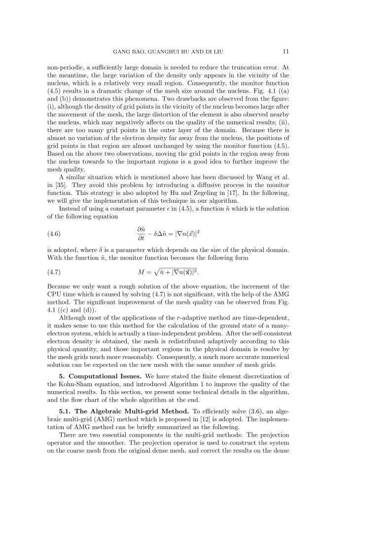
non-periodic, a sufficiently large domain is needed to reduce the truncation error. Atthe meantime, the large variation of the density only appears in the vicinity of thenucleus, which is a relatively very small region. Consequently, the monitor function(4.5) results in a dramatic change of the mesh size around the nucleus. Fig. 4.1 ((a)and (b)) demonstrates this phenomena. Two drawbacks are observed from the figure:(i), although the density of grid points in the vicinity of the nucleus becomes large afterthe movement of the mesh, the large distortion of the element is also observed nearbythe nucleus, which may negatively affects on the quality of the numerical results; (ii),there are too many grid points in the outer layer of the domain. Because there isalmost no variation of the electron density far away from the nucleus, the positions ofgrid points in that region are almost unchanged by using the monitor function (4.5).Based on the above two observations, moving the grid points in the region away fromthe nucleus towards to the important regions is a good idea to further improve themesh quality.

A similar situation which is mentioned above has been discussed by Wang et al.in [35]. They avoid this problem by introducing a diffusive process in the monitorfunction. This strategy is also adopted by Hu and Zegeling in [17]. In the following,we will give the implementation of this technique in our algorithm.

Instead of using a constant parameter ǫ in (4.5), a function n which is the solutionof the following equation

∂n

∂t− δ∆n = |∇n(~x)|2(4.6)

is adopted, where δ is a parameter which depends on the size of the physical domain.With the function n, the monitor function becomes the following form

M =√

n+ |∇n(~x)|2.(4.7)

Because we only want a rough solution of the above equation, the increment of theCPU time which is caused by solving (4.7) is not significant, with the help of the AMGmethod. The significant improvement of the mesh quality can be observed from Fig.4.1 ((c) and (d)).

Although most of the applications of the r-adaptive method are time-dependent,it makes sense to use this method for the calculation of the ground state of a many-electron system, which is actually a time-independent problem. After the self-consistentelectron density is obtained, the mesh is redistributed adaptively according to thisphysical quantity, and those important regions in the physical domain is resolve bythe mesh grids much more reasonably. Consequently, a much more accurate numericalsolution can be expected on the new mesh with the same number of mesh grids.

5. Computational Issues. We have stated the finite element discretization ofthe Kohn-Sham equation, and introduced Algorithm 1 to improve the quality of thenumerical results. In this section, we present some technical details in the algorithm,and the flow chart of the whole algorithm at the end.

5.1. The Algebraic Multi-grid Method. To efficiently solve (3.6), an alge-braic multi-grid (AMG) method which is proposed in [12] is adopted. The implemen-tation of AMG method can be briefly summarized as the following.

There are two essential components in the multi-grid methods: The projectionoperator and the smoother. The projection operator is used to construct the systemon the coarse mesh from the original dense mesh, and correct the results on the dense


(a) (b)

(c) (d)

Fig. 4.1. The demonstration of a slice of the 3-dimensional mesh in the plane (0, 0, 1) after themesh redistribution. (a) and (b) are generated with (4.5), while (c) and (d) are generated with (4.7).(b) and (d) show the detailed mesh around the nucleus of the whole mesh (a) and (c) respectively.

mesh by the solution obtained from the coarse mesh. There are two different way to getthe projection operator. One is the geometrical method which uses the information ofthe mesh to generate the projection operator. The other one is the algebraic methodwhich only use the information of linear system itself. We follow [12] to use thealgebraic method to construct the projection operator in the implementation.

The smoother in the multi-grid method is employed to damp out the relativelyhigh frequency parts of the numerical error of the result, with respect to the currentmesh level. In our implementation, the Gauss-Seidel iteration method is adopted. Tocancel the error effectively, a lower-upper process is implemented.

For the detailed algorithm of AMG, we refer to [12] and references therein. Herewe present a test which demonstrates that our implementation of AMG method workswell for solving the Poisson problem. For the problem, a cubic domain [−1, 1] ×[−1, 1]× [−1, 1] is chosen. The equation we want to solve is

−∆u = f.(5.1)


Since it is only a test, we use u = sin(πx)cos(πy)sin(πz) as the solution to setup theboundary condition and f respectively. Table 5.1 demonstrates the reliability of ourAMG solver.

Dof 63 365 2457 17969 137313l2 error 4.45e-01 2.37e-01 6.38e-02 1.63e-02 4.10e-03Conv. Or-der

0.91 1.89 1.97 1.99

Table 5.1

The l2 error and the corresponding convergence order of the the solution of (5.1). The finiteelement method is used to discretize the equation with piecewise linear approximation, and the linearsystem is solved by using the AMG method.

5.2. Boundary Conditions. To solve the equations (3.2) and (3.6), appropri-ate boundary conditions are needed. For (3.2), the zero Dirichlet boundary conditionsare adopted naturally. However, for (3.6), the zero Dirichlet boundary condition isno longer suitable. As we know that, far from a nucleus, the Hartree potential de-cays as N/r, where N is the electron number. Consequently, the simple use of zeroDirichlet boundary condition will introduce large truncation error on the boundary.To give the the evaluation of the Hartree potential on the boundary, (2.4) can be used

directly. However, it results in a O(N5

3 ) operations in the algorithm, which is notconsistent with O(N) of the AMG solver. To reduce the cost, a multipole expansionapproximation is employed for the boundary value. In the simulations, the followingthree terms, monopole, dipole and quadrupole, are used for the approximation,

VHartree(~x)|~x∈∂Ω ≈ Vmon(~x) + Vdip(~x) + Vquad(~x),

where

Vmon(~x) =1

4π|~x|

∫

Ω′

n(~x′)d~x′,

Vdip(~x) = − 1

4π|~x|2∫

Ω′

n(~x′)(~x · ~x′)d~x′,

Vquad(~x) =1

8π|~x|3∫

Ω′

n(~x′)(3(~x · ~x′)− |~x′|2)d~x′,

and in the above expressions, ~x = ~x/|~x|.Note that even the boundary value of Hartree potential is approximated by the

multipole expansion, a sufficiently large physical domain is still needed, because thenumerical accuracy of multipole expansion can only be guaranteed under the condition~x >> ~x′.

5.3. Linear Mixing Scheme. In the SCF iteration, we use a mixing strat-egy for updating electron density to guarantee the stability of the iteration. It isknown that in each SCF iteration, if the electron density which is obtained in thelast iteration is adopted directly to calculate the effective potential veff , the SCFiteration could be unstable. To fix this problem, many mixing schemes are pro-posed. Suppose we want to calculate electron density of k-th step of SCF itera-tion, the idea of these mixing schemes is to use the electron densities of previous


S steps, nP−S+1(~x), nP−S+2(~x), · · · , nP−1(~x), to generate an input electron density.This means we use

ninP = f(nP−S+1(~x), nP−S+2(~x), · · · , nP−1(~x))(5.2)

to calculate veff , then to find out new wave-functions and the new electron density.There are many mixing schemes such as linear mixing schemes which just linearlymixes the input and output electron density of the last step as the input of thecurrent step, and the GR-Pauly mixing scheme [9]. In the implementation, the simplelinear mixing scheme is used:

ninP = γnoutP−1 + (1− γ)ninP−1,(5.3)

where 0 < γ < 1. In the simulations, we always use γ = 0.7.Now we present the flow chart of the whole algorithm.

Flow Chart of the Algorithm 2

Input: The initial guess nini(~x) for the electron density, and ψinii

for the wave-function which is used in NSRQMCG method. Letnin(~x) = nini(~x).

S. 1 : With nin(~x), get the evaluation of vHartree by solving (3.6), and theevaluations of vext and vxc with (2.3) and (2.7) respectively. Thenthe generalized eigenvalue problem (3.2) is obtained.

S. 2 : Using NSRQMCG method to solve (3.2) to obtain the ψi andnout(~x). Note that the wave-function which obtained in the lastiteration is used as the initial guess for NSRQMCG method. If (3.9)is satisfied, goto Output; otherwise, goto S.3

S. 3 : Using Algorithm 1 to redistribute the grid points, then using (5.3)to get the new nin(~x), and goto S. 1.Output: the approximation of the ground state density, the totalenergy, and wave-functions.

6. Numerical Examples. In this section, the convergence of the proposedsolver is examined first. Then several atoms and molecules are simulated to showthe reliability and effectiveness of our solver. All simulations are implemented on aserver with Intel Xeon 2.66 GHz CPU and 64 GB of RAM.

Example 1: Solve the equation

−1

2∇2u− 1

|~x|u = λu(6.1)

with Algorithm 2. The lowest eigenvalue of this equation is −0.5.The above equation models the hydrogen atom. The physical domain is chosen

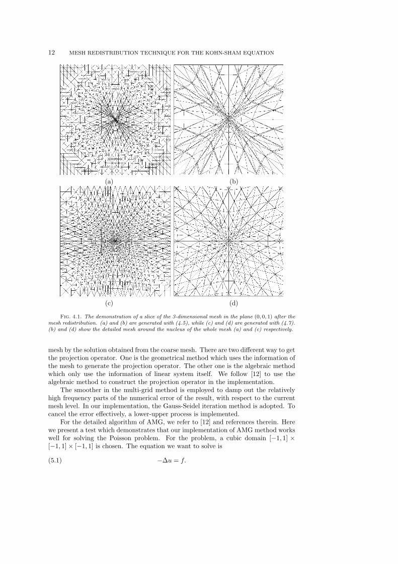
as [−10, 10]× [−10, 10]× [−10, 10]. The uniform mesh is refined successively from thecoarsest one which contains 63 grid points. The results are demonstrated in Fig. 6.1,which shows that both the convergence rate and the accuracy obtained with the meshredistribution are superior to that of the fixed uniform mesh. With the refinementof the mesh, the convergence order of solver with mesh redistribution reaches around1.9, which shows that the eigenvalue of this equation converges at the expected rate


0.001

0.01

0.1

1

100 1000 10000 100000

Err

or in

eig

enva

lue(

log)

Num. of Dof(log)

Fixed meshWith mesh redistribution

Fig. 6.1. Convergence rate of the eigenvalue with fixed uniform mesh and with mesh redistri-bution for Example 1. .

of the convergence for the linear finite element method.

Example 2: Calculate the total energy of the ground state of the helium and thelithium atoms by using the all-electron computation.

-2.9

-2.8

-2.7

-2.6

-2.5

-2.4

1000 10000 100000

Gro

und

stat

e en

ergy

(a. u

.)

Num. of Dof(log)


-7.4

-7.2

-7

-6.8

-6.6

-6.4

-6.2

-6

-5.8

-5.6

-5.4

-5.2

1000 10000 100000

Gro

und

stat

e en

ergy

(a. u

.)

Num. of Dof(log)


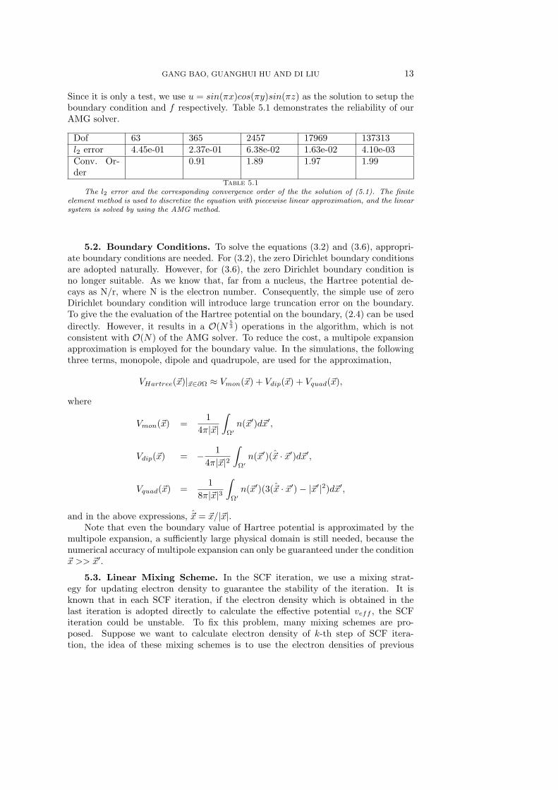
Fig. 6.2. The energies of the ground state of the helium atom (left) and the lithium atom (right)obtained on successively refined meshes, with fixed mesh and with mesh redistribution, for Example2.

For the all-electron calculation, the external potential (2.3) is very singular aroundthe nucleus. To resolve the external potential is very important for obtaining accu-rate ground state energy. Therefore, a rough radial mesh which is generated by theGMSH[1] is adopted. The coarsest mesh has 1867 nodes, and the mesh is successivelyrefined two times.

The results are shown in Fig. 6.2. It can be observed from the figure that, withthe successive refinement of the mesh, both results (with and without mesh redis-tribution) converges to the reference results, -2.835 for helium atom, and -7.335 for


lithium atom [20], respectively. It also can be observed that with the help of the meshredistribution technique, the numerical results are much more accurate than thatobtained from the fixed mesh with the same number of Dofs. It worth mentioningthat for both simulations, the results from using the mesh redistribution with 13924Dofs are almost the same to that from the fixed mesh with 180539 Dofs, which showsthe significant improvement on the solution quality the mesh redistribution techniquegives.

Example 3: Calculate the pseudo-atom energies of the lithium and the sodiumatoms, and the cohesive energies of these two metal dimers by using the smooth localEvanescent Core pseudopotential [14].

The Evanescent Core pseudopotential has the following form

V Iion(~x,RI) = − Z

Rc

[

1

y(1− (1 + βy)e−αy)−Ae−y

]

,

where Z is the number of valence electrons and y = |x − RI |/Rc. The element-dependent constants Rc and α can be found from [14]. In the above formula, theparameters β and A are given by

β =α3 − 2α

4(α2 − 1), A = 0.5α2 − αβ.

To calculate the pseudo-atom energy, the initial uniform mesh is adopted. Theresults are demonstrated in Table 6.1. It can be seen that our results give reasonableapproximations to the reference results. Especially for the sodium atom, with thehelp of the mesh redistribution, the solver using 17969 Dofs gives more accuratesolution than that using fixed uniform mesh with 137313 grid points. Furthermore,the CPU time is also studied for the simulation of the sodium atom, and the resultsare given in Table 6.2. It takes 207.20 CPU seconds to finish the calculating withthe mesh redistribution technique (17969 Dofs), while it is 587.11 CPU seconds forthe fixed uniform mesh case (137313 Dofs). It means that to achieve almost the samenumerical accuracy, mesh redistribution technique significantly improves the efficiencyof the algorithm.

Dof: 17969 Dof: 137313Metal Mesh redistribu-

tionFixed mesh Ref. [26]

Li -5.95 -5.95 -5.97Na -5.19 -5.18 -5.21

Table 6.1

The pseudo-atom energy (eV) using the Evanescent Core pseudopotential.

17969 Dof (mesh redistri-bution)

137313 Dof (fixed mesh)

CPU time (second) 207.20 587.11Table 6.2

The CPU seconds for the calculating the pseudo-atom energy of the sodium atom.


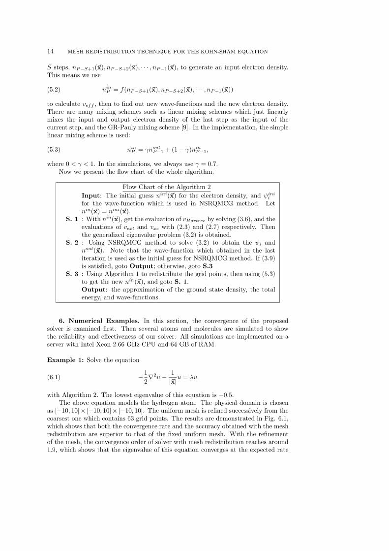
The cohesive energy of the lithium and the sodium dimers are also calculated,and the results are demonstrated in Table 6.3. A rough radial mesh is used as theinitial mesh in the simulation. The bond lengths of these two dimers are given fol-lowing [26]. From the results, we can see that the cohesive energies of both dimersare approximated reasonably. Again, compared with the fixed mesh case, the meshredistribution technique improves the solution quality successfully. Fig. 6.3 shows theoccupied valence molecular orbital of Na2, and its corresponding sliced mesh aroundthe orbital. It is obviously observed that the bond region is resolved by mesh grids,which shows that our mesh redistribution technique and the monitor function workvery well.

Mesh redistribu-tion

Fixed Mesh Ref. [26]

Li2 -0.49 -0.45 -0.52Na2 -0.45 -0.43 -0.46

Table 6.3

The cohesive energy (eV) of the lithium and the sodium dimers obtained by using the EvanescentCore pseudopotential.

Fig. 6.3. The occupied valence molecular orbital of Na2 (top), and the corresponding slicedmesh on the X-Y plane when Z = 0(bottom). The mesh redistribution technique is used.

Example 4: Calculate the ground state of the molecule BeH2, and demonstrate therelationship of the bond length of Be-H and the ground state energy of the moleculeBeH2.

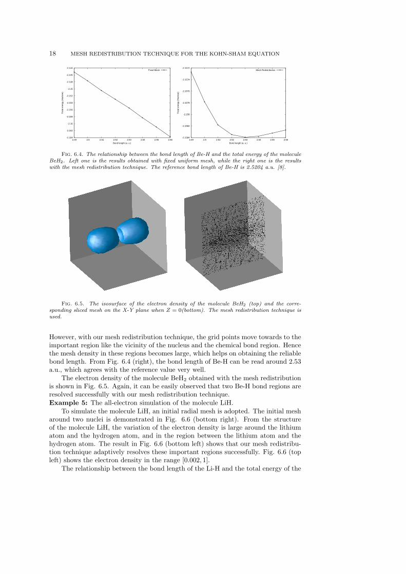
In the calculation, the smooth local Evanescent Core pseudopotential is adoptedfor the beryllium atom, while the all-electron is used for two hydrogen atoms. Theselection of the parameters in the pseudopotential for the beryllium atom is againfollowed [14]. Fig. 6.4 shows the relationship between the bond length of Be-H andthe total energy of the molecule BeH2, with and without the mesh redistributionrespectively. For the domain, a cube with the size [−20, 20] × [−20, 20] × [−20, 20]is chosen. This domain is discretized uniformly by 17969 grid points, which meansthat the mesh size is around 1.25 a.u.. This mesh size is too large to get a reliablenumerical results for the fixed mesh case. This can be demonstrated in Fig. 6.4 (left).


-2.164

-2.162

-2.16

-2.158

-2.156

-2.154

-2.152

-2.15

-2.148

-2.146

-2.144

2.49 2.5 2.51 2.52 2.53 2.54 2.55 2.56

Tot

al e

nerg

y (H

artr

ee)

Bond length (a. u.)

Fixed Mesh

-2.1584

-2.1582

-2.158

-2.1578

-2.1576

-2.1574

-2.1572

2.49 2.5 2.51 2.52 2.53 2.54 2.55 2.56

Tot

al e

nerg

y (H

artr

ee)

Bond length (a. u.)

Mesh Redistribution

Fig. 6.4. The relationship between the bond length of Be-H and the total energy of the moleculeBeH2. Left one is the results obtained with fixed uniform mesh, while the right one is the resultswith the mesh redistribution technique. The reference bond length of Be-H is 2.5204 a.u. [8].

Fig. 6.5. The isosurface of the electron density of the molecule BeH2 (top) and the corre-sponding sliced mesh on the X-Y plane when Z = 0(bottom). The mesh redistribution technique isused.

However, with our mesh redistribution technique, the grid points move towards to theimportant region like the vicinity of the nucleus and the chemical bond region. Hencethe mesh density in these regions becomes large, which helps on obtaining the reliablebond length. From Fig. 6.4 (right), the bond length of Be-H can be read around 2.53a.u., which agrees with the reference value very well.

The electron density of the molecule BeH2 obtained with the mesh redistributionis shown in Fig. 6.5. Again, it can be easily observed that two Be-H bond regions areresolved successfully with our mesh redistribution technique.Example 5: The all-electron simulation of the molecule LiH.

To simulate the molecule LiH, an initial radial mesh is adopted. The initial mesharound two nuclei is demonstrated in Fig. 6.6 (bottom right). From the structureof the molecule LiH, the variation of the electron density is large around the lithiumatom and the hydrogen atom, and in the region between the lithium atom and thehydrogen atom. The result in Fig. 6.6 (bottom left) shows that our mesh redistribu-tion technique adaptively resolves these important regions successfully. Fig. 6.6 (topleft) shows the electron density in the range [0.002, 1].

The relationship between the bond length of the Li-H and the total energy of the


ground state of the molecule LiH is also studied by using our solver. The result isshown in Fig. 6.6 (top right). It can be observed easily from the figure that the bondlength of the Li-H is around 3.01 a.u.. This agrees with the experimental value 3.016a.u. [18] very well.

Fig. 6.6. Top left: the electron density of the molecule LiH; Top right: the relationship betweenthe bond length of the Li-H and the total energy of the ground state of the molecule LiH; Bottomleft: the mesh with the mesh redistribution; Bottom right: initial mesh.

7. Concluding Remarks. We present a finite element method with an adap-tive mesh redistribution technique to solve the Kohn-Sham equation in this paper.The solver includes two main iterations. The first one is a SCF iteration which isfor the calculations of the self-consistent electron density on the current mesh. Inthis iteration, the Kohn-Sham equation is discretized by the standard finite elementmethod. In the Hamiltonian operator, the Hartree potential is obtained by solvingthe Poisson equation with AMG method. The LDA is used to give the exchange-correlation potential. For the external potential, both the all-electron and the localpseudopotential are considered. The generalized eigenvalue problem is solved usingthe NSRQMCG method.


After the self-consistent electron density is obtained, an adaptive mesh redistri-bution technique, which is based on the harmonic mapping, is proposed to optimizethe mesh quality. The harmonic mapping is obtained iteratively with a given mon-itor function, which depends on the gradient of the electron density. To guaranteethe mesh quality, the monitor function is smoothed by a method which based on thediffusive mechanism. The results show that the mesh quality is significantly improvedwith our mesh redistribution strategy.

The numerical experiments successfully demonstrate the convergence of our solver.Furthermore, the numerical accuracy and the CPU time are also studied. Results showthat with the help of the mesh redistribution technique, both the numerical accuracyof the solution and the efficiency of the algorithm are significantly improved, comparedwith the fixed mesh case.

In this paper, we mainly focus on the ground state of atoms and molecules.To obtain the accurate ground state energy and the electron density, using a well-designed non-uniform mesh is proven a good idea by [30, 22]. It is expected that thatour solver may be extended to time-dependent density functional theory (TDDFT)case. In the TDDFT, if the external potential is not strong, the system can be studiedby the perturbative methods . Under this situation, the perturbed system is not faraway from the ground state, which means that the well-designed, fixed mesh is stillapplicable. However, this may not be the case for a very strong external potential.For example, for the simulations of the high-order harmonic generations and themulti-photon ionizations. In these cases, the electronic structure may be dramaticallychanged. This may cause difficulty for just using a fixed mesh. Consequently, the meshredistribution technique which is proposed in this paper may help on this issue. Withour adaptive technique, the region with the large gradient of the electron density willalways be resolved adaptively, which can effectively improve the numerical accuracyof solutions. Some preliminary numerical results have shown the advantages of oursolver on the TDDFT calculations. The research findings will be reported on ourforthcoming paper.

Acknowledgements. The authors would like to thank Prof. Chao Yang (LawrenceBerkeley National Laboratory) for his helpful comments, suggestions on this work.The research was supported in part by the NSF Focused Research Group grant DMS-0968360. This research of G. Bao was also supported in part by the NSF grantsDMS-0908325, CCF-0830161, EAR-0724527, the ONR grant N00014-09-1-0384 and aspecial research grant from Zhejiang University.

REFERENCES

[1] http://geuz.org/gmsh/.[2] http://cms.mpi.univie.ac.at/vasp.[3] http://www.abinit.org.[4] http://www.caam.rice.edu/software/ARPACK.[5] W. E. Arnoldi, The principle of minimized iterations in the solution of the matrix eigenvalue

problem, Quarterly of Applied Mathematics, 9 (1951), pp. 17–29.[6] A. D. Becke, Hartree-Fock exchange energy of an inhomogeneous electron gas, International

Journal of Quantum Chemistry, 23 (1983), pp. 1915–1922.[7] , A new inhomogeneity parameter in density-functional theory, The Journal of Chemical

Physics, 109 (1998), pp. 2092–2098.[8] P. F. Bernath, A. Shayesteh, K. Tereszchuk, and R. Colin, The vibration-rotation em-

mision spectrum of free beh2, Science, 297 (2002), p. 1323.[9] D. R. Bowler and M. J. Gillan, An efficient and robust technique for achieving self consis-


tency in electronic structure calculations, Chemical Physics Letters, 325 (2000), pp. 473–476.

[10] E. J. Bylaska, M. Holst, and J. H. Weare, Adaptive finite element method for solving theexact Kohn-Sham equation of density functional theory, Journal of Chemical Theory andComputation, 5 (2009), pp. 937–948.

[11] D. M. Ceperley and B. J. Alder, Ground state of the electron gas by a stochastic method,Physical Reivew Letters, 45 (1980), pp. 566–569.

[12] A. J. Cleary, R. D. Falgout, V. E. Henson, J. E. Jones, T. A. Manteuffel, S. F.

Mccormick, G. N. Miranda, and J. W. Ruge, Robustness and scalability of algebraicmultigrid, SIMA Journal on Scientific Computing, 21 (2000), pp. 1886–1908.

[13] Y. N. Di, R. Li, and T. Tang, A general moving mesh framework in 3D and its application forsimulating the mixture of multi-phase flows, Communications in Computational Physics,3 (2008), pp. 582–602.

[14] C. Fiolhais, J.P. Perdew, S. Q. Armster, J.M. Maclaren, and M. Brajczewska, Domi-nant density parameters and local pseudopotentials for simple metals, Physical Review B,51 (1995), pp. 14001–14011.

[15] G. Gambolati, F. Sartoretto, and P. Florian, An orthogonal accelerated deflation tech-nique for large symmetric eigenproblems, Computer Methods in Applied Mechanics andEngineering, 94 (1992), pp. 13–23.

[16] P. Hohenberg and W. Kohn, Inhomogeneous electron gas, Physical Review, 136 (1964),pp. B864–B871.

[17] G. H. Hu and P. A. Zegeling, Simulating finger phenomenon in porous media with a movingfinite element method, Journal of Computational Physics, 230 (2011), pp. 3249–3263.

[18] K. Huber and G. Herzberg, Molecular Spectra and Molecular Structure. IV. Constants ofDiatomic Molecules, Van nostrand Reinhold: New York, 1979.

[19] W. Kohn and L. J. Sham, Self-consistent equations including exchange and correlation effects,Physical Reivew, 140 (1965), pp. A1133–A1138.

[20] S. Kotochigova, Z. H. Levine, E. L. Shirley, M. D. Stiles, and C. W. Clark, Local-density-functional calculations of the energy of atoms, Physical Review A, 55 (1997),pp. 191–199.

[21] G. Kresse and J. Furthmuller, Efficient iterative shcemes for ab initio total-energy calcu-lations using a plane-wave basis set, Physical Reivew B, 54 (1996), pp. 11169–11186.

[22] L. Lehtovaara, V. Havu, and M. Puska, All-electron density functional theory and time-dependent density functional theory with high-order finite elements, Journal of ChemicalPhysics, 131 (2009), p. 054103.

[23] R. Li, T. Tang, and P. W. Zhang, Moving mesh methods in multiple dimensions based onharmonic maps, Journal of Computational Physics, 170 (2001), pp. 562–588.

[24] , A moving mesh finite element algorithm for singular problems in tow and three spacedimensions, Journal of Computational Physics, 177 (2002), pp. 365–393.

[25] S. K. Ma and K. A. Brueckner, Correlation energy of an electron gas with a slowly varyinghigh density, Physical Review, 165 (1968), pp. 18–31.

[26] F. Nogueira, C. Fiolhais, J.S. He, and A. Rubio, Transferability of a local pseudopotentialbased on solid-state electron density, Journal of Physics: Condensed Matter, 8 (1996),pp. 287–302.

[27] J. P. Perdew and Y. Wang, Accurate and simple density functional for the electronicexchange energy: Generalized gradient approximation, Physical Reivew B, 33 (1986),pp. 8800–8802.

[28] , Accurate and simple analytical representation of the electron-gas correlation energy,Physical Review B, 45 (1992), pp. 13244–13249.

[29] Y. Saad, J. R. Chelikowsky, and S. M. Shontz, Numerical methods for electronic structurecalculations of materials, SIAM Review, 52 (2010), pp. 3–54.

[30] P. Suryanarayana, V. Gavini, T. Blesgen, K. Bhattacharya, and M. Ortiz, Non-periodicfinite-element formulation of Kohn-Sham density functional theory, Journal of the Me-chanics and Physics of Solids, 58 (2010), pp. 256–280.

[31] T. Tang, Moving mesh methods for computational fluid dynamics, Contemporary Mathemat-ics, 383 (2005).

[32] T. Torsti, T. Eirola, J. Enkovaara, T. Hakala, P. Havu, V. Havu, T. Hoynalanmaa,

J. Ignatius, M. Lyly, I. Makkonen, T. T. Rantala, J. Ruokolainen, K. Ruotsalainen,

E. Ras”anen, H. Saarikoski, and M. J. Puska, Three real-space discretization techniquesin electronic structure calculations, Physica Status Solidi (b), 243 (2006), pp. 1016–1053.

[33] E. Tsuchida and M. Tsukada, Adaptive finite-element method for electronic-structure calcu-lations, Physical Reivew B, 54 (1996), pp. 7602–7605.


[34] H. Y. Wang and R. Li, Mesh sensitivity for numerical solutions of phase-field equations usingr-adaptive finite element methods, Communications in Computational Physics, 3 (2008),pp. 357–375.

[35] H. Y. Wang, R. Li, and T. Tang, Efficient computation of dendritic growth with r-adaptivefinite element methods, Journal of Computational Physics, 227 (2008), pp. 5984–6000.

[36] C. Yang, J. C. Meza, B. Lee, and L. W. Wang, Kssolv-a matlab toolbox for solving theKohn-Sham equations, ACM Transactions on Mathematical Software, 36 (2009).

[37] D. E. Zhang, L. H. Shen, A. H. Zhou, and X. G. Gong, Finite element method for solv-ing Kohn-Sham equations based on self-adaptive tetrahedral mesh, Physics Letter A, 372(2008), pp. 5071–5076.

NUMERICAL SOLUTION OF THE KOHN-SHAM …NUMERICAL SOLUTION OF THE KOHN-SHAM EQUATION BY FINITE...

Documents

Transcript of NUMERICAL SOLUTION OF THE KOHN-SHAM …NUMERICAL SOLUTION OF THE KOHN-SHAM EQUATION BY FINITE...