Numerical Solution of Fully Nonlinear Elliptic Equations ... · Numerical Solution of Fully...

Numerical Solution of Fully Nonlinear Elliptic

Equations by Bohmer’s Method

Oleg Davydov∗ Abid Saeed†

April 16, 2013

Abstract

We present an implementation of Bohmer’s finite element method

for fully nonlinear elliptic partial differential equations on convex polyg-

onal domains, based on a modified Argyris element and Bernstein-

Bezier techniques. Our numerical experiments for several test prob-

lems, involving the classical Monge-Ampere equation and an uncon-

ditionally elliptic equation, confirm the convergence and error bounds

predicted by Bohmer’s theoretical results.

1 Introduction

Numerical solution of fully nonlinear elliptic partial differential equations is atopic of intensive research and great practical interest, see [7]. The motivationbehind this interest is the presence of these equations in different fields ofscience and engineering including differential geometry [2], fluid mechanics[18] and optimal transportation [5].

Several numerical methods have been recently proposed in the literaturefor the fully nonlinear equations, in particular finite difference [13, 20] andfinite element type methods [6, 14, 15, 8, 3, 4, 19]. The most of these methodsare restricted to the equations of Monge-Ampere type, such as the Monge-Ampere equation, the equation of Gaussian curvature and Pucci’s equation.

Bohmer’s method [6, 7] allows solving the Dirichlet problem for any fullynonlinear elliptic equations of second order. It is based on a finite element dis-cretisation of the linearised elliptic equations, with C1 finite element spaces

∗Department of Mathematics and Statistics, University of Strathclyde, 26 Richmond

Street, Glasgow G1 1XH, Scotland, UK, [email protected]†Department of Mathematics and Statistics, University of Strathclyde, 26 Richmond

Street, Glasgow G1 1XH, Scotland, UK, [email protected]

1

that admit a stable splitting into the subspace satisfying zero boundary con-ditions and its complement. This method does not require any variationalformulation of the fully nonlinear equation. Full theoretical justification ofthe method is given in [6, 7], including a proof of convergence and errorbounds. However, no numerical results have been provided.

This paper presents the first implementation of Bohmer’s method basedon a modified Argyris finite element space with a stable splitting developedin [11, 12]. Our construction makes use of the Bernstein-Bezier techniques forpiecewise polynomials [17, 21]. These techniques are widespread in geometricmodelling, and currently gain more attention in the finite element method be-cause of a number of desirable properties, in particular optimal complexityof the element system matrix assembly [1]. Note that C1 conforming dis-cretisations based on a variational formulation of either the Monge-Ampereequation or a fouth order quasilinear equation resulting from a singular per-turbation of the Monge-Ampere equation have been recently explored in[3, 4, 15]. Neither of these discretisations is equivalent to Bohmer’s method.In particular, the spline element method of [3, 4] uses Lagrange multipliersto enforce inter-element smoothness and boundary conditions by solving asaddle point problem, rather than relying on a stable splitting of a C1 finiteelement space.

Our numerical experiments include several standard test problems forthe Monge-Ampere equation on a square, an example for a non-rectangularconvex polygonal domain, and an unconditionally elliptic equation. Thenumerical results confirm the theoretical error bounds given in [6, 7].

The paper is organised as follows. Section 2 is devoted to the formulationof Bohmer’s method. In Section 3 we recall our construction of the modifiedArgyris space [12] and provide the details of the numerical implementation ofa stable local basis admitting a stable splitting. In Section 4 we discuss theimplementation of Bohmer’s method, including the assembly of the systemmatrix for the linearised elliptic equations arising in each step of Newtoniteration. Finally, Section 5 is devoted to the numerical experiments.

2 Bohmer’s Method for Elliptic Equations

2.1 Fully Nonlinear Elliptic Operators

Let Ω be a bounded domain in Rn and let G be a second order differential

operator of the formG(u) = G(·, u,∇u,∇2u),

where G is a real valued function defined on a domain Ω × Γ such that

Ω ⊂ Ω ⊂ Rn and Γ ⊂ R × R

n × Rn×n,

2

and ∇u,∇2u denote the gradient and the Hessian of u, respectively. Thepoints in Ω × Γ are denoted by w = (x, z, p, r), with x ∈ Ω, z ∈ R, p =[pi]

ni=1 ∈ R

n, r = [rij]ni,j=1 ∈ R

n×n, to indicate the product structure of thisset. We denote by D(G) the domain of the operator G.

The operator G is said to be elliptic in a subset Γ ⊂ Ω × Γ if the matrix

[ ∂ eG∂rij

(w)]ni,j=1 is well defined and positive definite for all w ∈ Γ [7, 16]. If G

is a linear function of (z, p, r) for each fixed x, then G is a linear differential

operator. Under suitable restrictions on G, classes of quasilinear and semi-linear differential operators are obtained [7, p. 80], but in general G may befully nonlinear.

In the neighborhood of a fixed function u ∈ D(G) the linear ellipticoperator G′(u) is defined by

G′(u)u =∂G

∂z(w)u +

n∑

i=1

∂G

∂pi

(w)∂iu +n∑

i,j=1

∂G

∂rij

(w)∂i∂ju, (1)

where w = (x, u(x),∇u(x),∇2u(x)) is a function of x ∈ Ω, and ∂i denotesthe partial derivative with respect to the i-th variable. Note that G′(u) isthe Frechet derivative of G if G is Frechet differentiable at u.

Many nonlinear elliptic operators and corresponding equations G(u) = 0are important for applications. A standard example of a fully nonlinearequation is the Monge-Ampere equation on Ω ⊂ R

2, given by

GMA(u) := det(∇2u) − f(x) = 0, f(x) > 0 for x ∈ Ω.

We consider the Dirichlet problem for the operator G: Find u such that

G(u) = 0, x ∈ Ω, (2)

u = φ, x ∈ ∂Ω, (3)

where φ is a continuous function defined on ∂Ω. Under certain assumptions,including the exterior sphere condition for ∂Ω and sufficient smoothness ofG, this problem has a unique solution u ∈ C2(Ω)∩C(Ω) [16, Theorem 17.17].

Note that the Monge-Ampere operator GMA is elliptic in subsets Γ satisfying

Γ ⊂ Ω × R × Rn × r ∈ R

n×n : r is positive definite.

Therefore there exists a unique convex solution of GMA(u) = 0, whereas itis known that the Monge-Ampere equation has another, concave solution [9,Chapter 4].

3

2.2 Spline Spaces and Stable Splitting

As usual in the finite element method, the discretisation of the Dirichletproblem is done with the help of spaces of piecewise polynomial functions(splines). Let be a triangulation of a polyhedral domain Ω ⊂ R

n, thatis a partition of Ω into simplices such that the intersection of every pair ofsimplices is either empty or a common face. The space of multivariate splinesof degree d and smoothness r is defined by

Srd() = s ∈ Cr(Ω) : s|T ∈ Pd for all simplices T in , (4)

where d > r ≥ 0 and Pd is the space of polynomials of total degree d inn variables. Recall that the star of a vertex v of , denoted by star(v) =star1(v), is the union of all simplices T ∈ attached to v. We define starj(v),j ≥ 2, inductively as the union of the stars of all vertices of contained instarj−1(v), and star(T ) as the union of the stars of all vertices of the simplexT .

Let hh∈H be a family of triangulations of Ω, where h is the maximumedge length in h. The triangulations in the family are said to be quasi-uniform if there is an absolute constant c > 0 such that ρT ≥ ch for allT ∈ h, where ρT denotes the radius of the inscribed sphere of the simplexT .

Let Sh ⊂ Srd(h) be a linear space with basis s1, . . . , sN and dual linear

functionals λ1, . . . , λN : Sh → R such that λisj = δij . This basis is stableand local if there are three constants m ∈ N and C1, C2 > 0 independent ofh such that (a) supp sk is contained in starm(v) for some vertex v of h, (b)‖sk‖L∞(Ω) ≤ C1, k = 1, . . . , N , and (c) |λks| ≤ C2‖s‖L∞(supp sk), k = 1, . . . , N ,for all s ∈ Sh, see [10, 11] and [7, Section 4.2.6].

To handle the Dirichlet boundary condition (3), the following subspaceof Sh is important:

Sh0 :=

s ∈ Sh : s|∂Ω = 0

.

We say that Sh admits a stable splitting

Sh = Sh0 + Sh

b ,

if there is a stable local basis s1, . . . , sN for Sh that can be split into twoparts

s1, . . . , sN = s1, . . . , sN0 ∪ sN0+1, . . . , sN,

where s1, . . . , sN0 and sN0+1, . . . , sN are bases for the subspaces Sh

0 andSh

b , respectively. Note that the space Shb is not uniquely defined by the pair

Sh, Sh0 . It was shown in [11, 12] (see also [7, Section 4.2.6]) how the stable

splitting can be achieved for a modified Argyris finite element space.

4

2.3 Bohmer’s Method

Let u = u be the solution of (2)–(3). According to [6, 7], its approximationuh ≈ u is sought as a solution of the following problem: Find uh ∈ Sh suchthat

(G(uh), vh)L2(Ω) = 0 ∀vh ∈ Sh0 , and (5)

(uh, vhb )L2(∂Ω) = (φ, vh

b )L2(∂Ω) ∀vhb ∈ Sh

b , (6)

where (·, ·) denotes the inner products in the respective Hilbert spaces. SinceSh

0 and Shb are finite dimensional linear spaces, the problem (5)–(6) is equiv-

alent to a system of algebraic equations with respect to the coefficients of uh

in a basis of Sh.

Theorem 1 ([7, Theorem 5.2]) Let Ω be a bounded convex polyhedral do-main, and let G : D(G) → L2(Ω), with D(G) ⊂ H2(Ω), satisfy Con-dition H of [7, Section 5.2.3]. Assume that G is continuously differen-tiable in the neighbourhood of an isolated solution u of (2)–(3), such thatu ∈ D(G) ∩ Hℓ(Ω), ℓ > 2, and G′(u) : D(G) ∩ H1

0 (Ω) → L2(Ω) is bound-edly invertible. Furthermore, assume that the spline spaces Sh ⊂ S1

d(h),d ≥ ℓ − 1, on quasi-uniform triangulations h possess stable local bases andstable splitting Sh = Sh

0 + Shb , and include polynomials of degree ℓ− 1. Then

the problem (5)–(6) has a unique solution uh ∈ Sh as soon as the maximumedge length h is sufficiently small. Moreover,

‖u − uh‖H2(Ω) ≤ Chℓ−2‖u‖Hℓ(Ω).

Note that, in particular, all conditions of Theorem 1 are satisfied by theMonge-Ampere operators, where D(GMA) = C2(Ω), see [7, Example 3.26].

The nonlinear problem (5)–(6) can be solved iteratively by a Newtonmethod as suggested in [6], where the initial guess uh

0 ∈ Sh satisfies theboundary condition

(uh0 , v

hb )L2(∂Ω) = (φ, vh


b ,

and the sequence of approximations uhkk∈N of uh is generated by

uhk+1 = uh

k − wh, k = 0, 1, . . . ,

with wh ∈ Sh0 being the solution of the linear elliptic problem:

Find wh ∈ Sh0 such that (G′(uh

k)wh, vh)L2(Ω) = (G(uh

k), vh)L2(Ω) ∀vh ∈ Sh

0 .

Clearly, wh can be found by using the standard finite element method. Undersome additional assumptions on G, it is proved in [6, Theorem 9.1] that uh

i

converges to uh quadratically. Note that in the case when G(u) is onlyconditionally elliptic (e.g. elliptic only for a convex u for Monge-Ampereequation) the ellipticity of the above linear problem is only guaranteed foruh

k sufficiently close to the exact solution u.

5

3 C1 Finite Elements with Stable Splitting

3.1 Bernstein-Bezier Techniques

This section is devoted to the key concepts of the Bernstein-Bezier techniqueswe rely upon in our implementation of the finite element spaces suitable forBohmer’s method. A comprehensive treatment of these techniques can befound in [17]. We restrict to the case of two variables.

Let Ω ⊂ R2 be a polygonal domain and a triangulation of Ω. For a

given d ≥ 1, let Dd, :=⋃

T∈ Dd,T be the set of domain points, where

Dd,T :=

ξijk =

iv1 + jv2 + kv3

d

i+j+k=d

for each triangle T := 〈v1, v2, v3〉 in . We will use the following terminologyfor certain subsets of Dd,T . We refer to the set

Rn(v) := ξijk ∈ Dd, : i = d − n , 0 ≤ n ≤ d,

of domain points as the ring of radius n around the vertex v and refer to theset

Dn(v) :=

n⋃

m=0

Rm(v)

as the disk of radius n around the vertex v.Recall that every v ∈ R

2 can be uniquely represented in the form

v =

3∑

i=1

bivi,

3∑

i=1

bi = 1,

where the components of the triplet (b1, b2, b3) are called the barycentric coor-dinates of v relative to the triangle T := 〈v1, v2, v3〉. Barycentric coordinatesare linear functions of v, and the functions

Bdijk(v) :=

d!

i!j!k!bi1b

j2b

k3, i + j + k = d,

are the Bernstein-Bezier basis polynomials of degree d associated with trian-gle T . Every polynomial p of total degree d can be written uniquely as

p =∑

i+j+k=d

cijkBdijk,

where cijk are the Bezier coefficients of p. For each s ∈ S0d() and ξ = ξijk ∈

Dd, we denote by cξ the coefficient cijk of the restriction of s to any triangle

6

T ∈ containing ξ. (Because of the continuity of s the coefficient cξ doesnot depend on the particular choice of such triangle.)

A key concept for dealing with spline spaces in Bernstein-Bezier form isthat of a minimal determining set. The set M ⊂ Dd, is a determining setfor a linear space S ⊂ S0

d() if

s ∈ S and cξ = 0 ∀ξ ∈ M ⇒ s = 0,

and M is a minimal determining set (MDS) for the space S if there is nosmaller determining set. Then dim S equals the cardinality #M of M .

Usually subspaces S ⊂ S0d() are defined with the help of certain smooth-

ness conditions which can be explicitly written down as linear equations in-volving the coefficients cξ, ξ ∈ Dd,. For a given minimal determining setM for S, if we assign values to the coefficients cξξ∈M

, then the remainingcoefficients cη, η ∈ Dd,\M of a spline s ∈ S can be computed using thesmoothness conditions. Hence, an MDS M can be used to construct theM-basis sξξ∈M for S by requiring that the Bezier coefficients cη, η ∈ M ,of sξ satisfy cξ = 1 and cη = 0 for all η ∈ M \ ξ.

We now introduce the concept of a stable and local MDS, which appliesto algorithms of constructing an MDS for any triangulation of a given family,for example for all triangulations in two variables with a given lower boundon the minimum angle of the triangles. Let

Γη := ξ ∈ M : cη depends on cξ , η ∈ Dd,\M,

where we say that cη depends on cξ, ξ ∈ M , if the value of cη for a splines ∈ S is changed when we change the value of cξ. This simply means thatthe coefficient cη of the basis spline sξ is not zero. A minimal determining setM for a space S is said to be local if there exists an absolute integer constantℓ not depending on such that

Γη ⊂ starℓ(Tη) ∀η ∈ Dd,\M,

where Tη is a triangle containing η. Moreover, M is called stable if thereexists a constant K which may depend only on d, ℓ and the smallest angleθ in the triangulation such that

|cη| ≤ K maxξ∈Γη

|cξ| ∀η ∈ Dd,\M.

If M is a stable local MDS, then the corresponding M-basis of S is stableand local in the sense of Section 2.2. A stable splitting of this basis canoften be achieved by an appropriate splitting of the MDS, which leads to thefollowing definition.

7

Definition 2 Assume that the space S ⊂ S0d() has a stable local MDS M

and letS0 := s ∈ S : s|∂Ω = 0 . (7)

The MDS M is said to admit a stable splitting if M is the disjoint union oftwo subsets M0, Mb ⊂ M such that

S0 = s ∈ S : cξ = 0 ∀ξ ∈ Mb (8)

and M0 and Mb are stable local MDS for the spaces S0 and Sb, respectively,where

Sb := s ∈ S : cξ = 0 ∀ξ ∈ M0 . (9)

Note that if M is a stable local MDS, and M = M0 ∪ Mb is a disjointunion, then it is a stable splitting as soon as (8) holds.

If M admits a stable splitting, then S = S0 +Sb and it is easy to see that

sξξ∈M = sξξ∈M0∪ sξξ∈Mb

is a stable splitting of the stable local basis sξξ∈M .

3.2 Modified Argyris Space

Recall that the superspline spaces Sr,ρd (), r ≤ ρ ≤ d, of Sr

d() are definedas

Sr,ρd () = s ∈ Sr

d() : s ∈ Cρ(v) ∀v ∈ V , (10)

where V is the set of all vertices of .The Argyris finite element space is obtained by choosing d = 5, r = 1

and ρ = 2 in (10). Now for each v ∈ V , let Tv be one of the triangles sharingthe vertex v and let Mv := D2(v) ∩ Tv. For each edge e of the triangulation, let Te := 〈v1, v2, v3〉 be one of the triangles sharing the edge e := 〈v2, v3〉and let Me :=

ξTe

122

. Then from [17, Theorem 6.1] we have

Theorem 3 The dimension of the Argyris finite element space is given bydim S1,2

5 () = 6#V + #E, and

M =⋃

v∈V

Mv ∪⋃

e∈E

Me (11)

is a stable local minimal determining set for S1,25 ().

The modified Argyris space S [11, 12] is given by

S :=s ∈ S1

5() : s ∈ C2(v), for all interior vertices v of

. (12)

8

We now introduce some further notation that will help us to describe a stablelocal MDS for S. Let VI and VB denote the sets of interior and boundaryvertices of , respectively, and let EI and EB represent the sets of interiorand boundary edges, such that V = VI ∪VB, E = EI ∪EB. Let, furthermore,Ev = e1, e2, · · · , en denote all edges of emanating from a vertex v ∈ V ,in counterclockwise order. For each ei, let ξi be the (unique) domain pointin R2(v)∩ ei, i = 1, . . . , n. For each v ∈ V , we choose a triangle Tv as above,where we assume in addition that Tv shares an edge with the boundary of Ωif v ∈ VB. We define Mv and Me as above, and set

Mv := Mv ∪ ξ1, ξ2, · · · , ξn.

Theorem 4 ([12, Theorem 4]) The dimension of the modified Argyris spaceS is given by dim S = 6#VI + #E +

∑v∈VB

(4 + #Ev), and

M :=⋃

v∈VI

Mv ∪⋃

e∈E

Me ∪⋃

v∈VB

Mv. (13)

is a stable local MDS for S.

We now split M into two disjoint subsets M0 and Mb as follows. Let

(⋃

v∈VI

Mv ∪⋃

e∈E

Me

)⊂ M0, (14)

and let all points of M lying on the boundary be in Mb. Also let

R2(v) ∩ Mv\e1, en ∈ M0, for each v ∈ VB.

Now only one point in R1(v)∩ Mv, for each v ∈ VB, is not assigned to eitherM0 or Mb. We denote this point by ξv. Where ξv belongs depends on thegeometry of the boundary edges attached to v.

• If boundary edges attached to v are non-collinear, then ξv ∈ Mb.

• If boundary edges attached to v are collinear, then ξv ∈ M0.

Now we are in position to formulate the theorem about stable splitting forthe modified Argyris space.

Theorem 5 ([12]) M = M0 ∪ Mb is the stable splitting of the stable localMDS M for S.

Stable splitting of an MDS is impossible for the standard Argyris spacein general, as the following result shows.

9

Theorem 6 ([12]) No MDS for the Argyris space can be stably split onarbitrary triangulations.

As we will see in the next section, a key step in the implementation of thefinite element stiffness matrices using Bernstein-Bezier techniques is the com-putation of the Bezier coefficients of the basis splines sξξ∈M correspondingto an MDS M . We therefore conclude this section by providing Algorithm 1that gives all details of this computation for the basis splines of the modifiedArgyris space.

4 Implementation of Bohmer’s Method

In this section we describe in detail our implementation of Bohmer’s methodusing Bernstein-Bezier techniques. We study the numerical approximationof Dirichlet problem (2)-(3) for a fully nonlinear equation of second order.

Discretisation

Recall that h is a quasi-uniform triangulation of a convex polygonal domainΩ ⊂ R

2. As discussed in Section 2, solving the nonlinear problem (2)-(3)by Bohmer’s method amounts to running a Newton-Kantorovich iterationscheme to get a sequence

uh

k

k∈Z+

of approximations of u generated by

uhk+1 = uh

k − wh, k = 0, 1, . . . , (17)

where wh ∈ Sh0 is the solution of the linear elliptic problem: Find wh ∈ Sh

0

such that(G′(uh

k)wh, vh)L2(Ω) = (G(uh

k), vh)L2(Ω) ∀vh ∈ Sh

0 , (18)

where G′ is the linearisation (1) of the nonlinear operator G. We solve thislinear equation by using the standard Galerkin finite element method withthe modified Argyris space Sh on h as an approximating space, with thestable splitting Sh = Sh

0 + Shb according to Theorem 5.

After a standard transformation to the weak form, (18) is translated intothe following problem: Find wh ∈ Sh

0 such that for all vh ∈ Sh0 ,

∫

Ω

∇wh · A∇vhdx +

∫

Ω

vhb · ∇whdx +

∫

Ω

cwhvhdx =

∫

Ω

fvhdx, (19)

where A =[

∂ eG∂rij

(whk)]2

i,j=1, b =

[∂ eG∂pi

(whk)]2

i=1, f = G(uh

k) and c = ∂ eG∂z

(whk).

If (s1, . . . , sN0) is a basis of Sh

0 , then, as usual in the finite element method,(19) results in the linear system

(S + Bt + M)a = L (20)

10

Algorithm 1 Compute Bezier coefficients of a basis spline sξ, ξ ∈ M .

Require: Given ξ, initialize cη : η ∈ D5, by zeros and set cξ = 1. Recallthat Te is triangle sharing the edge e ∈ E. Let Te be the other trianglesharing the edge e if e ∈ EI .

Ensure: Compute cη ∀η ∈ D\M.1. if ξ ∈ Mv, v ∈ VI then2. Find triangles Tκk

κ=1 attached to vertex v, arranged in anti-clockwiseorder, with T1 := Tv.

3. Move anti-clockwise by computing cν , ν ∈ D2(v) ∩ Tκ+1 from knowncoefficients cη, η ∈ D2(v) ∩ Tκ, κ = 1, · · · , k − 1, using C1 and C2

smoothness conditions [17, Lemma 2.30]. We write these smoothnessconditions explicitly. Let T1 := 〈v, v2, v1〉 and T2 := 〈v3, v, v1〉 are twoof the triangles attached to vertex v then we compute c′ν , ν ∈ D2(v)∩T2

from known coefficients cη, η ∈ D2(v) ∩ T1 as follows

c′131 = b1c401 + b2c311 + b3c302, (15)

c′140 = b1c500 + b2c410 + b3c401, (16)

c′230 = b21c500 + 2b1b2c410 + b2

2c320 + 2b2b3c311 + b23c302 + 2b3b1c401,

where (b1, b2, b3) are barycentric coordinates of v3 w.r.to T1.4. For each edge e ∈ Ev. Let the edge e := 〈v, v1〉 be shared by trian-

gles Te := 〈v, v2, v1〉 and Te := 〈v3, v, v1〉. We compute cTe

122 using C1

smoothness condition over e [17, Lemma 2.30]

cTe

122 = b1c302,

where (b1, b2, b3) are barycentric coordinates of v3 w.r.to Te and c302 isknown for ξ302 ∈ D2(v).

5. else if ξ ∈ Mv, v ∈ VB then6. Do as in 2) by choosing T1 := Tv be one of the boundary triangles

attached to v.7. Compute cν , ν ∈ D2(v) ∩ Tκ+1 \Mv from known coefficients cη, η ∈

D2(v)∩Tκ, κ = 1, · · · , k−1, using the same C1 smoothness conditions(15)-(16).

8. Do as in 4) only for e ∈ Ev\EB.9. else if ξ ∈ Me, e ∈ EI then

10. Let the edge e := 〈v1, v2〉 is shared by triangles Te := 〈v1, v4, v2〉 and

Te := 〈v3, v1, v2〉. Then ξ := ξTe

212 and we compute cTe

122 with the help ofcTe

212 = 1 using C1 smoothness condition over e given by

cTe

122 = b3,

where (b1, b2, b3) are barycentric coordinates of v3 w.r.to Te.11. end if 11

where a is the vector of the coefficients in the expansion wh =∑N0

i=1 aisi, andS, B, M and L are the stiffness, convection and mass matrices and the loadvector, respectively, with the entries, for i, j = 1, . . . , N0, defined as

Sij =

∫

Ω

∇si·A∇sjdx, Bij =

∫

Ω

sjb·∇sidx, Mij =

∫

Ω

csisjdx, Li =

∫

Ω

fsidx.

It is worth emphasising that we do not use these formulae directly to computethe system matrices. Before we describe how we compute them let us definea transformation matrix T required for this.

Transformation Matrix

Let TκNt

κ=1 be the triangles in h with some fixed ordering. Recall that anyspline s ∈ Sh restricted to the triangle Tκ can be written in the form

s|Tκ=

∑

i+j+k=5

cijkB5ijk,

where cijk are Bezier coefficients of s on Tκ. Let CTκ, κ = 1, · · · , Nt, denote

the row vector of these coefficients cijk of s on Tκ, where we use the lexi-cographic order as in [17, p. 23] to arrange these coefficients. That is, thetriples of the indices (i, j, k) are arranged by the ordering function

q(i, j, k) =

(j + k + 1

2

)+ k + 1.

Let V(s) be a row vector of all CTκ’s, κ = 1, · · · , Nt, for a spline s, ordered

according to the triangles TκNt

κ=1,

V(s) =[CT1

,CT2, · · · ,CTNt

].

Now, if we construct a matrix by taking these vectors V(si) for the basissplines s1, . . . , sN0

as its rows, then this matrix is our desired transformationmatrix T ,

T = [V(s1)t, . . . ,V(sN0

)t]t.

Let S5(h) denote the space of all discontinuous quintic splines over thesame triangulation h. Clearly, T t represents the transformation that mapsthe vector cξξ∈M corresponding to s ∈ Sh

0 onto the array of the coefficients

of s in the basis of the space S5(h) defined by the quintic Bernstein basispolynomials B5

ijk on all triangles.

Now let S = diag(STκ

, Tκ ∈ h), B = diag

(BTκ

, Tκ ∈ h)

and M =

diag(MTκ

, Tκ ∈ h)

be the block matrices with blocks defined by

STκ=

∫

Tκ

∇B5ijk·A∇B5

rstdx, BTκ=

∫

Tκ

B5ijkb·∇B5

rstdx, MTκ=

∫

Tκ

cB5ijkB

5rstdx.

12

Then we can compute the system matrices in (20) by using the relations

S = T ST t, B = T BT t, M = T MT t.

Note that this method of computing the system matrices is particularlyefficient as it is shown in [1] that the matrices S, B and M can be computed inoptimal complexity (constant cost per entry) even for high polynomial orders,and the matrix T is sparse because the basis splines are locally supported.

Boundary Conditions

As discussed in Section 2, in order to impose the non-homogeneous boundaryconditions we require that the initial guess uh

0 ∈ Sh, satisfy the followingcondition

(uh0 , v

hb )L2(∂Ω) = (φ, vh


b .

Now if (s1, . . . , sN0, sN0+1, . . . , sN) is the M-basis for the space Sh and (sN0+1, . . . , sN)

is a basis for Shb , then the above boundary condition is reduced to the matrix

equationMbCb = Lb,

where Mb =[∫

∂Ωsisjds

]Ni,j=N0+1

and Lb =[∫

∂Ωφsids

]Ni=N0+1

. It is important

to mention that si|e, e ∈ E, are univariate polynomials and they keep theunivariate BB-form [17, Remark 2.4]. Moreover, there is an explicit formulafor integration of the product of two polynomials in BB-form given by

∫

e

sisjds =|e|11

5∑

α=0β=0

cαc′β

(5α

)(5β

)(

10α+β

) ,

where |e| is the length of e,

si|e =

5∑

α=0

cαB5α and sj |e =

5∑

β=0

c′βB5β ,

with B5α =

(5α

)tα(1 − t)5−α, α = 0, . . . , 5, being the univariate quintic Bern-

stein polynomials on the edge e.Now consider

∫

e

φsids =

∫

e

φ

5∑

α=0

cαB5αds =

5∑

α=0

cα

∫

e

φB5αds. (21)

Thus, computing the entries for Lb is reduced to approximating the Bernstein-Bezier moments µ5

α(φ) =∫

eφB5

αds of φ using an appropriate quadrature rule

13

[1]. We use Gauss-Legendre 6-points rule to approximate the moments µ5α(φ)

which returns the exact solution for polynomials of order up to 11. Note that,unlike using C0 elements, here some degrees of freedom for Sh

b lie inside thedomain Ω, see Theorem 5. Thus it would be difficult to impose the boundaryconditions merely by interpolating the function φ at the points correspondingto the degrees of freedom lying on the boundary.

5 Numerical Results

This section is devoted to the numerical results for several fully nonlinearproblems, involving the Monge-Ampere equation and an unconditionally el-liptic problem considered in [19]. The numerics for these problems confirmthe convergence and the theoretical error bounds of Theorem 1.

5.1 The Monge-Ampere equation

The Dirichlet problem for the Monge-Ampere equation is given by

GMA(u) = det(∇2u) − g(x) = 0, x ∈ Ω

u = φ, x ∈ ∂Ω(22)

where g and φ are given functions with g > 0 on Ω required to keep theproblem elliptic. The weak formulation (19) of the linearised problem in thiscase is to find wh ∈ Sh

0 such that∫

Ω

∇wh · A∇vhdx =

∫

Ω

fvhdx, for all vh ∈ Sh0 , (23)

with A = cof(∇2uhk) as b = 0, c = 0 and f = GMA(uh

k) = det(∇2uhk) − g(x),

where cof(M) denotes the cofactor of a 2 × 2 matrix M . As a result we areleft with the stiffness matrix and load vector to solve the linear system

SC = L,

for the unknown vector of Bezier coefficients C of wh.As Monge-Ampere equation is elliptic only for convex functions, we need

the initial guess to be convex as well. In [13, Remark 2.1] it has been shownthat (22) and the Poisson-Dirichlet problem

∆u = 2√

g, x ∈ Ω

u = φ, x ∈ ∂Ω(24)

are closely related. Therefore we use the approximation solution of thePoisson-Dirichlet problem (24) as an initial guess for the Newton scheme

14

(17). The initial guess obtained this way performs very well in our experi-ments. However, we get much faster convergence of the Newton method byusing this initial guess only on initial mesh, whereas on the refined mesheswe take a quasi-interpolant [17, Section 5.7] of the solution from previouslevel as an initial guess. We call this a multilevel approach.

The first three and the fifth test problems are standard benchmark prob-lems for (22) over Ω = (0, 1)2 considered in many paper on the numericalsolution of the Monge-Ampere equation. In this case h is the uniform tri-angulation obtained by first dividing the domain into squares of side length hand then drawing in the diagonals parallel to the line x2 = x1. In the fourthtest problem a non-rectangular domain is considered.

1. As the first test problem we solve (22) for the data

g(x) = (1 + |x|2)e|x|2, in Ω,

φ(x) = e1

2|x|2 ∀x ∈ ∂Ω,

where |x| =√

x21 + x2

2. With this data the exact solution to the prob-

lem is u(x) = e1

2|x|2 ∈ C∞(Ω). The numerical results are presented

in Table 1. They confirm the convergence rate O(h4) in the H2-normpredicted by Theorem 1, where ℓ = 6 as we are using polynomials ofdegree 5. Moreover, as expected, we observe the convergence rates ofO(h6) and O(h5) in the L2 and H1 norms, respectively. The first rowof the table shows the errors for the initial guess. In addition to theerrors, Table 1 presents the number of Newton iterations (N) on eachmesh, the L2-norm of the residuals r := ‖G(uh

k)‖L2(Ω), and the size

‖p‖L2(Ω) of the L2-projection p of G(uhk) on the space Sh

0 . The pro-jection p is found as a solution of the system MCp = L, where M isthe mass matrix and Cp is the vector of coefficients of the expansion ofp in the M0-basis. The size of the projection measures how well theapproximate solution uh

k solves the problem (5). We observe that thenumber of Newton iterations is extremely small thanks to the fact thatthe initial guess is chosen by the multilevel approach. The size of theresidual is close to the H2-norm error, as one can expect, and the size ofthe projection is close to the unit round-off initially, and gets larger onfurther refinement levels, obviously due to growing condition numbersof the system matrices.

2. Second test problem is defined by

g(x) =R2

(R2 − |x|2)2∀x ∈ Ω, with R ≥

√2,

φ(x) = −√

R2 − |x|2 ∀x ∈ ∂Ω,

15

Table 1: Errors of approximate solution and rate of convergence for thefirst test problem, N denotes the number of Newton’s iterations, r :=‖G(uh

k)‖L2(Ω) is the size of the residual, and ‖p‖L2(Ω) is the size of the L2-

projection of G(uhk) on Sh

0 .

h L2-error rate H1-error rate H2-error rate N r ‖p‖L2(Ω)

initial 5.78e-3 3.25e-2 2.66e-1 9.64e-11 1.17e-4 1.03e-3 1.74e-2 2 5.15e-2 2.30e-15

1/2 4.77e-6 4.6 7.75e-5 3.7 2.25e-3 3.0 1 5.14e-3 1.74e-141/4 1.92e-7 4.6 7.04e-6 3.5 3.32e-4 2.8 1 8.28e-4 9.44e-141/8 2.42e-9 6.3 1.65e-7 5.4 1.58e-5 4.4 1 3.93e-5 3.89e-131/16 4.31e-11 5.8 6.61e-9 4.6 1.20e-6 3.7 1 3.56e-6 1.79e-121/32 6.60e-13 6.0 1.95e-10 5.1 7.45e-8 4.0 1 2.04e-7 7.38e-121/64 1.14e-14 5.9 7.28e-12 4.7 6.06e-9 3.6 1 1.66e-8 2.83e-111/128 8.16e-15 0.5 2.96e-13 4.6 3.73e-10 4.0 1 1.07e-9 1.06e-10

in (22). The exact solution is u(x) = −√

R2 − |x|2. The function

g(x) has singularity at R =√

2 and u ∈ W 1p (Ω), 1 ≤ p < 4 for this

value of R, lacking H2-regularity. The method diverges for R =√

2,in line with Bohmer’s theory that guarantees convergence only if thesolution is in H2. But for R >

√2 we have u ∈ C∞(Ω) and again,

in Table 2 and Table 3 for two different values of R, the results showthe same behaviour as in the first problem. The tables confirm thatthe more the value of R is away from singularity the faster convergenceis achieved. Note that in this experiments much higher accuracy isattained as compared to the results in [13] for the same test problem.

3. Third test problem is defined by

g(x) =1

|x| ∀x ∈ Ω,

φ(x) =(2|x|) 3

2

3∀x ∈ ∂Ω.

in the Monge-Ampere equation (22). The difference to the previous

problems is that the exact solution u(x) =(2|x|) 3

2

3is not infinitely

differentiable, even u /∈ C2(Ω). However, as u ∈ Hs(Ω), for all s < 52,

we expect convergence order O(h5

2 ) in L2-norm. The results, in Table4, confirm this.

16

Table 2: Errors of approximate solution and rate of convergence for thesecond test problem with R =

√2 + .1. The meaning of the last three

columns is the same as in Table 1.


initial 2.00e-3 1.67e-2 2.69e-1 1.02e01 2.34e-3 1.25e-2 2.15e-1 2 5.91e-1 1.92e-15

1/2 1.70e-4 3.8 1.57e-3 3.0 7.32e-2 1.6 2 1.68e-1 7.89e-151/4 6.01e-6 4.8 1.58e-4 3.3 1.75e-2 2.1 2 3.80e-2 2.92e-141/8 1.72e-7 5.1 1.31e-5 3.6 3.17e-3 2.5 1 6.61e-3 1.34e-131/16 3.92e-9 5.4 8.10e-7 4.0 4.05e-4 3.0 1 8.44e-4 5.04e-131/32 1.02e-10 5.3 3.71e-8 4.4 3.53e-5 3.5 1 7.23e-5 2.07e-121/64 1.93e-12 5.7 1.41e-9 4.7 2.80e-6 3.7 1 5.49e-6 8.45e-12

Table 3: Errors of approximate solution and rate of convergence for thesecond test problem with R =

√2 + 2.



1/2 1.28e-8 5.9 2.50e-7 4.6 7.85e-6 3.4 1 2.49e-6 7.68e-151/4 4.33e-10 4.9 1.72e-8 3.9 8.65e-7 3.2 1 2.58e-7 2.97e-141/8 6.66e-12 6.0 4.94e-10 5.1 9.78e-8 4.1 1 1.46e-8 1.49e-131/16 1.10e-13 5.9 1.75e-11 4.8 3.36e-9 3.8 1 1.00e-9 5.71e-131/32 7.67e-15 3.6 5.53e-13 4.9 2.12e-10 3.9 1 6.17e-11 2.25e-12

4. Fourth test problem. This problem is different from the others becausewe consider a non-rectangular domain Ω, as Bohmer’s method is ap-plicable to any convex polygonal domain. Let Ω be bounded by thelines

x1 = ±0.75, x2 = ±0.75, and |x2| − |x1| = 1,

see Figure 1(left), which also includes the initial triangulation. Wegenerate a sequence of meshes by the uniform refinement, where eachtriangle is split into 4 similar subtriangles. This test problem is for (22)with the same data as in first test problem. Again we choose initialguess by the multilevel approach and use a solution of (24) on the firstlevel. The numerics again show the same rate of convergence as for therectangular domains, see Table 5. The graph of approximate solution

17

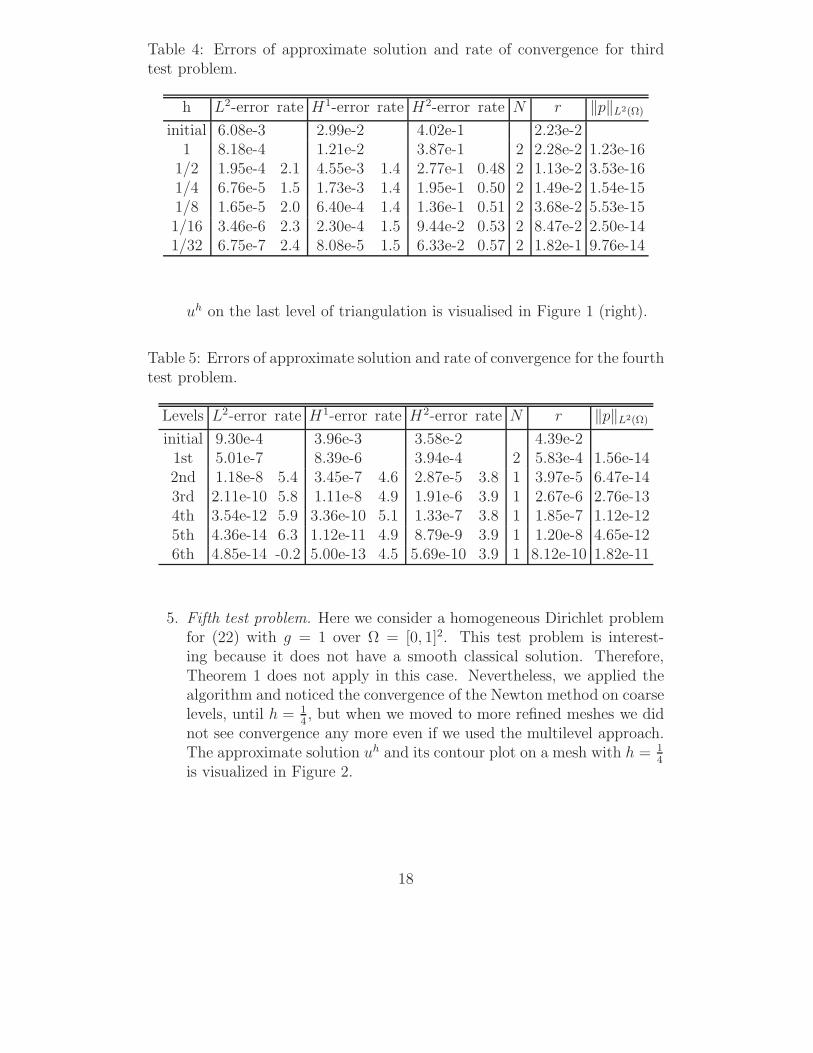
Table 4: Errors of approximate solution and rate of convergence for thirdtest problem.



1/2 1.95e-4 2.1 4.55e-3 1.4 2.77e-1 0.48 2 1.13e-2 3.53e-161/4 6.76e-5 1.5 1.73e-3 1.4 1.95e-1 0.50 2 1.49e-2 1.54e-151/8 1.65e-5 2.0 6.40e-4 1.4 1.36e-1 0.51 2 3.68e-2 5.53e-151/16 3.46e-6 2.3 2.30e-4 1.5 9.44e-2 0.53 2 8.47e-2 2.50e-141/32 6.75e-7 2.4 8.08e-5 1.5 6.33e-2 0.57 2 1.82e-1 9.76e-14

uh on the last level of triangulation is visualised in Figure 1 (right).

Table 5: Errors of approximate solution and rate of convergence for the fourthtest problem.

Levels L2-error rate H1-error rate H2-error rate N r ‖p‖L2(Ω)

initial 9.30e-4 3.96e-3 3.58e-2 4.39e-21st 5.01e-7 8.39e-6 3.94e-4 2 5.83e-4 1.56e-142nd 1.18e-8 5.4 3.45e-7 4.6 2.87e-5 3.8 1 3.97e-5 6.47e-143rd 2.11e-10 5.8 1.11e-8 4.9 1.91e-6 3.9 1 2.67e-6 2.76e-134th 3.54e-12 5.9 3.36e-10 5.1 1.33e-7 3.8 1 1.85e-7 1.12e-125th 4.36e-14 6.3 1.12e-11 4.9 8.79e-9 3.9 1 1.20e-8 4.65e-126th 4.85e-14 -0.2 5.00e-13 4.5 5.69e-10 3.9 1 8.12e-10 1.82e-11

5. Fifth test problem. Here we consider a homogeneous Dirichlet problemfor (22) with g = 1 over Ω = [0, 1]2. This test problem is interest-ing because it does not have a smooth classical solution. Therefore,Theorem 1 does not apply in this case. Nevertheless, we applied thealgorithm and noticed the convergence of the Newton method on coarselevels, until h = 1

4, but when we moved to more refined meshes we did

not see convergence any more even if we used the multilevel approach.The approximate solution uh and its contour plot on a mesh with h = 1

4

is visualized in Figure 2.

18

−0.8 −0.6 −0.4 −0.2 0 0.2 0.4 0.6 0.8−0.8

−0.6

−0.4

−0.2

0

0.2

0.4

0.6

0.8

Figure 1: Non-rectangular domain Ω for fourth test problem with initialtriangulation (left) and approximate solution uh on the last level of triangu-lation (right).

0 0.20.4 0.6 0.8

1

0

0.5

1

−0.25

−0.2

−0.15

−0.1

−0.05

0

10 20 30 40 50 60 70 80 90 100

10

20

30

40

50

60

70

80

90

100

Figure 2: Approximate solution uh of test 5 and its contour plot, h = 14

19

5.2 Second Example

Consider the problem suggested in [19]

G2(u) = u311 + u3

22 + u11 + u22 − g(x) = 0, x ∈ Ω

u = φ, x ∈ ∂Ω(25)

where uii = (∂i)2u, i = 1, 2. This problem is unconditionally elliptic, i.e.

the operator G2 is elliptic for any function u ∈ D(G2) = C2(Ω). Note thatCondition H of [7] is satisfied in this example. The last of our test problemsis for (25) in the domain Ω = [−1, 1]2, with the data given by

g(x) = ((4x21 − 2)3 + (4x2

2 − 2)3)e−3|x|2 + (4|x|2 − 4)e−|x|2, ∀x ∈ Ω,

φ(x) = e−|x|2 ∀x ∈ ∂Ω.

The matrix A in this case is

A =

[3u2

11 + 1 00 3u2

22 + 1

]

and b = 0, c = 0. Note that A is strictly positive definite for any function u.The triangulations h with side length h are generated the same way as forΩ = [0, 1]2 in Section 5.1.

To find an initial guess for the Newton method on the initial triangulation2 we use the approximate solution of the Laplace-Dirichlet problem

∆u = 0, x ∈ Ω,

u = φ, x ∈ ∂Ω,(26)

whereas on the subsequent refinement levels we use the multilevel approachas described in Section 5.1. Note that the method was divergent with initialguess generated by (26) for h ≤ 1

2.

The results are presented in Table 6. They confirm the theoretical con-vergence rate of Bohmer’s method. However, we see a very slow convergenceof Newton’s iterations in this example, compare N in Tables 1–6. We also ob-serve the difference in the behaviour of ‖p‖L2(Ω), which seems to indicate thatNewton method does not find a solution of (5). This phenomenon requiresfurther investigation.

References

[1] M. Ainsworth, G. Andriamaro, and O. Davydov, Bernstein-Bezier finiteelements of arbitrary order and optimal assembly procedures, SIAM J.Sci. Comp., 33 (2011), 3087–3109.

20

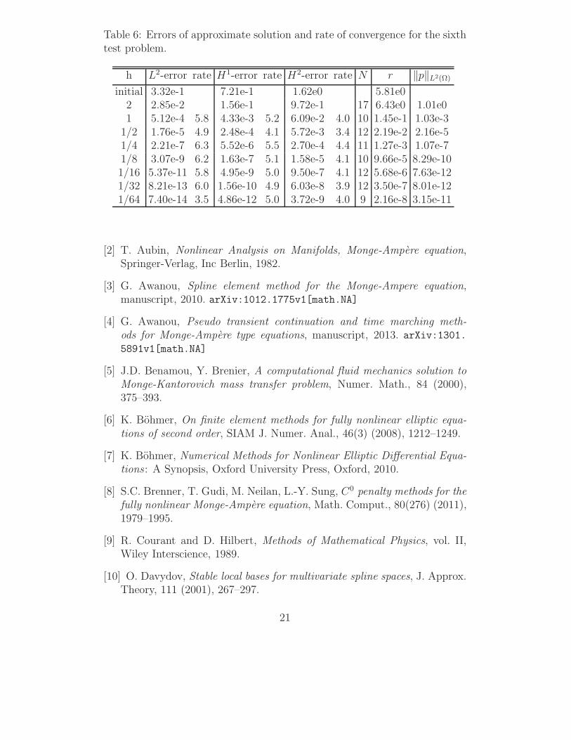
Table 6: Errors of approximate solution and rate of convergence for the sixthtest problem.


initial 3.32e-1 7.21e-1 1.62e0 5.81e02 2.85e-2 1.56e-1 9.72e-1 17 6.43e0 1.01e01 5.12e-4 5.8 4.33e-3 5.2 6.09e-2 4.0 10 1.45e-1 1.03e-3

1/2 1.76e-5 4.9 2.48e-4 4.1 5.72e-3 3.4 12 2.19e-2 2.16e-51/4 2.21e-7 6.3 5.52e-6 5.5 2.70e-4 4.4 11 1.27e-3 1.07e-71/8 3.07e-9 6.2 1.63e-7 5.1 1.58e-5 4.1 10 9.66e-5 8.29e-101/16 5.37e-11 5.8 4.95e-9 5.0 9.50e-7 4.1 12 5.68e-6 7.63e-121/32 8.21e-13 6.0 1.56e-10 4.9 6.03e-8 3.9 12 3.50e-7 8.01e-121/64 7.40e-14 3.5 4.86e-12 5.0 3.72e-9 4.0 9 2.16e-8 3.15e-11

[2] T. Aubin, Nonlinear Analysis on Manifolds, Monge-Ampere equation,Springer-Verlag, Inc Berlin, 1982.

[3] G. Awanou, Spline element method for the Monge-Ampere equation,manuscript, 2010. arXiv:1012.1775v1[math.NA]

[4] G. Awanou, Pseudo transient continuation and time marching meth-ods for Monge-Ampere type equations, manuscript, 2013. arXiv:1301.5891v1[math.NA]

[5] J.D. Benamou, Y. Brenier, A computational fluid mechanics solution toMonge-Kantorovich mass transfer problem, Numer. Math., 84 (2000),375–393.

[6] K. Bohmer, On finite element methods for fully nonlinear elliptic equa-tions of second order, SIAM J. Numer. Anal., 46(3) (2008), 1212–1249.

[7] K. Bohmer, Numerical Methods for Nonlinear Elliptic Differential Equa-tions : A Synopsis, Oxford University Press, Oxford, 2010.

[8] S.C. Brenner, T. Gudi, M. Neilan, L.-Y. Sung, C0 penalty methods for thefully nonlinear Monge-Ampere equation, Math. Comput., 80(276) (2011),1979–1995.

[9] R. Courant and D. Hilbert, Methods of Mathematical Physics, vol. II,Wiley Interscience, 1989.

[10] O. Davydov, Stable local bases for multivariate spline spaces, J. Approx.Theory, 111 (2001), 267–297.

21

[11] O. Davydov, Smooth finite elements and stable splitting, Berichte“Reihe Mathematik” der Philipps-Universitat Marburg, 2007-4 (2007).An adapted version has appeared as [7, Section 4.2.6].

[12] O. Davydov and A. Saeed, Stable splitting of bivariate splines spaces byBernstein-Bezier methods, in J.-D. Boissonnat et al. (Eds.): Curves andSurfaces - 7th International Conference, Avignon, France, June 24-30,2010 LNCS 6920, Springer-Verlag, 2012, pp. 220–235.

[13] E.J. Dean, R. Glowinski, Numerical methods for fully nonlinear ellip-tic equations of the Monge-Ampere type, Computer Methods in AppliedMechanics and Engineering, 195 (2006), 1344-1386.

[14] X. Feng, M. Neilan, Mixed finite element methods for the fully nonlinearMonge-Ampere equation based on the vanishing moment method, SIAMJ. Numer. Anal., 47(2) (2009) 1226–1250.

[15] X. Feng, M. Neilan, Vanishing moment method and moment solution forfully nonlinear second order partial differential equations, J. Sci. Comput.,38(1) 78-98, 2009.

[16] D. Gilbarg and N. S. Trudinger, Elliptic partial differential equations ofsecond order, Springer-Verlag, Berlin, 2001.

[17] M. J. Lai and L. Schumaker, Spline Functions on Triangulations, Cam-bridge University Press, 2007.

[18] F.X. Le Dimet, M. Ouberdous, Retrieval of balanced fields: an optimalcontrol method, Tellus, (45A) (1993), 449–461.

[19] O. Lakkis, T. Pryer, A non-variational finite element methodfor the nonlinear elliptic problems, manuscript, 2012. arXiv:1103.

2970v4[math.NA].

[20] A. Oberman, Wide stencil finite difference schemes for the ellipticMonge-Ampere equations and functions of the eigenvalues of the Hessian,Discrete Contin. Dyn. Syst. Ser B 10(1) (2008), 221–238.

[21] L. L. Schumaker, Computing bivariate splines in scattered data fittingand the finite element method, Numer. Algorithms, 48 (2008), 237–260.

22

Numerical Solution of Fully Nonlinear Elliptic Equations ... · Numerical Solution of Fully...

Documents

Transcript of Numerical Solution of Fully Nonlinear Elliptic Equations ... · Numerical Solution of Fully...