683

2011,23(6):683-696 DOI: 10.1016/S1001-6058(10)60166-7

NUMERICAL SIMULATIONS OF HIGHLY NONLINEAR STEADY AND UNSTEADY FREE SURFACE FLOWS*

YANG Chi, HUANG Fuxin, WANG Lijue Center for Computational Fluid Dynamics, George Mason University, Fairfax, Virginia, USA, E-mail: cyang@gmu.edu WAN De-cheng State Key Laboratory of Ocean Engineering, School of Naval Architecture, Ocean and Civil Engineering, Shanghai Jiao Tong University, Shanghai 200240, China (Received November 10, 2011, Revised November 25, 2011) Abstract: A numerical simulation model based on an open source Computational Fluid Dynamics (CFD) package–Open Field Operation and Manipulation (OpenFOAM) has been developed to study highly nonlinear steady and unsteady free surface flows. A two-fluid formulation is used in this model and the free surface is captured using the classical Volume Of Fluid (VOF) method. The incompressible Euler/Navier-Stokes equations are solved using a finite volume method on unstructured polyhedral cells. Both steady and unsteady free surface flows are simulated, which include: (1) a submerged NACA0012 2-D hydrofoil moving at a constant speed, (2) the Wigley hull moving at a constant speed, (3) numerical wave tank, (4) green water overtopping a fixed 2-D deck, (5) green water impact on a fixed 3-D body without or with a vertical wall on the deck. The numerical results obtained have been compared with the experimental measurements and other CFD results, and the agreements are satisfactory. The present numerical model can thus be used to simulate highly nonlinear steady and unsteady free surface flows. Key words: finite volume, Volume Of Fluid (VOF) method, nonlinear free surface flows, wave body interaction Introduction

Highly nonlinear steady and unsteady free sur- face flow problems are often encountered in marine and offshore industry. For instance, ships and offshore structures can suffer serious damage due to green water impact loading resulting from highly nonlinear free surface flows. With the rapid development of computer hardware and software, numerical studies of highly nonlinear free surface flows, including brea- king waves and green water on deck, have become increasingly popular. Over the years, various nume- rical methods have been developed to study the highly nonlinear free surface flow problems associated with the ship advancing at a constant speed[1-3], breaking

* Project supported by the National Natural Science Foun- dation of China (Grant Nos. 50739004, 11072154), the Foun- dation of State Key Laboratory of Ocean Engineering, Shanghai Jiao Tong University (Grant No. GKZD 010053-11). Biography: YANG Chi, Female, Ph. D., Professor

waves[4,5], sloshing[6-8], green water on deck[9-16]. Some success has been achieved, but further investi- gation is needed. In general, it is still a challenge to model and investigate highly nonlinear steady or un- steady free surface flow problems, especially green water problems, numerically to gain a quantitative understanding of the problems.

The Center for Computational Fluid Dynamics (CFD) at George Mason University (GMU) has deve- loped an incompressible Euler/Navier-Stokes solver operating on adaptive, unstructured grids and coupled it with a Volume Of Fluid (VOF) technique to model highly nonlinear wave body interactions. The solver has been applied to various marine and offshore engi- neering applications, including sloshing, large ampli- tude ship motions with slamming and green water on deck, coupling of ship motion and tank sloshing, ship- ship interactions with or without mooring cables[8,12,13,17-21]. In order to foster the easy collabo- ration between different institutions, the CFD Center at GMU has been working collaboratively with State Key Laboratory of Ocean Engineering at Shanghai

684

Jiao Tong University on the further development of a free, open source CFD software package–Open Field Operation and Manipulation (OpenFOAM) (http://www.openfoam.org) over the past years. The main subject of this paper is to develop numerical models with OpenFOAM and perform detailed valida- tions for the fully nonlinear steady and unsteady free surface flow problems.

OpenFOAM is an object oriented C++ toolbox for solving various systems of partial differential equations using the finite volume method on arbitrary control volume shapes and configurations. It includes preprocessing (grid generator, converters, manipula- tors, case setup), postprocessing (using OpenSource Paraview), and many specialized CFD solvers (http://www.openfoam.org). The features in OpenFOAM are comparable to what is available in the major commercial CFD codes. Some of the more specialized features that are included in OpenFOAM are: sliding grid, moving meshes, two-phase flow and fluid-structure interaction. Since OpenFOAM is an open-source code, it is possible to gain control over the exact implementations of different features and it is reasonably straightforward to implement new models and fit them into the whole code structure. Many researchers are using OpenFOAM, which allows international exchange of development.

Based on the successful application of OpenFOAM in various free surface flow applications (www.openfoamworkshop.org), two of the OpenFOAM solvers, interFoam and interDyMFoam, are further developed in this study to investigate highly nonlinear steady and unsteady free surface flows. A VOF phase-fraction based interface captu- ring approach is used to model the free surface. The volume fraction of water (0 for air and 1 for water) is propagated by a convection equation and is solved as a scalar function. The interface between air and water is determined by an interpolated value of 0.5. For interDyMFoam, optional mesh motion and mesh topo- logy changes (including adaptive re-meshing) are fea- tured. Thus, interFoam is selected for the steady flow simulation while interDyMFoam is chosen for the simulations of the unsteady wave tank and wave-body interactions. The turbulence modeling is generic (i.e., laminar, RANS or LES) for both of them. The laminar assumption is selected in this study for both steady and unsteady flows.

Detailed validations are carried out, which include: (1) a submerged NACA0012 2-D hydrofoil moving at a constant speed, (2) the Wigley hull moving at a constant speed, (3) numerical wave tank, (4) green water overtopping a fixed 2-D deck and (5) green water impact on a fixed 3-D body without or with a vertical wall on the deck. The numerical results obtained have been compared with the experimental measurements and other CFD results, and the satisfa-

ctory agreements are obtained. The present paper is organized as follows:

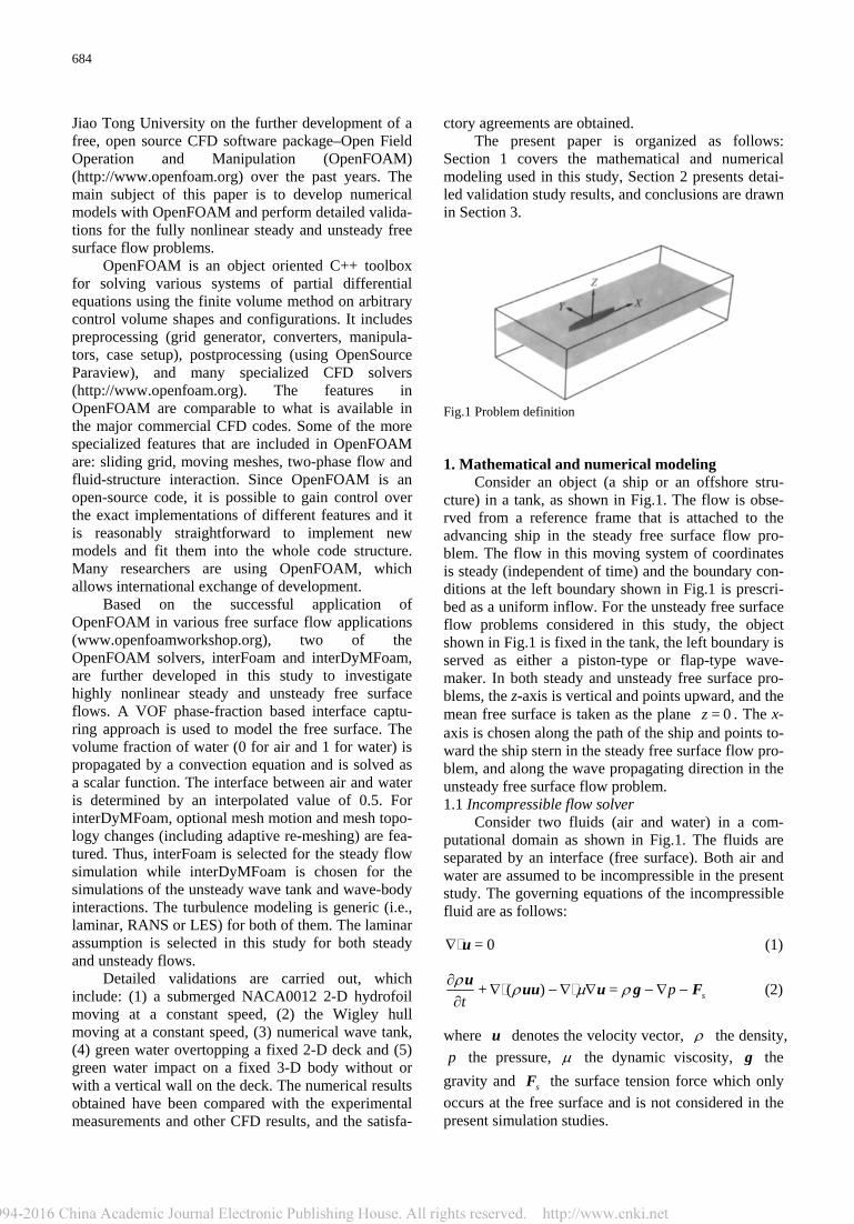
Section 1 covers the mathematical and numerical modeling used in this study, Section 2 presents detai- led validation study results, and conclusions are drawn in Section 3. Fig.1 Problem definition 1. Mathematical and numerical modeling

Consider an object (a ship or an offshore stru- cture) in a tank, as shown in Fig.1. The flow is obse- rved from a reference frame that is attached to the advancing ship in the steady free surface flow pro- blem. The flow in this moving system of coordinates is steady (independent of time) and the boundary con- ditions at the left boundary shown in Fig.1 is prescri- bed as a uniform inflow. For the unsteady free surface flow problems considered in this study, the object shown in Fig.1 is fixed in the tank, the left boundary is served as either a piston-type or flap-type wave- maker. In both steady and unsteady free surface pro- blems, the z-axis is vertical and points upward, and the mean free surface is taken as the plane = 0z . The x- axis is chosen along the path of the ship and points to- ward the ship stern in the steady free surface flow pro- blem, and along the wave propagating direction in the unsteady free surface flow problem. 1.1 Incompressible flow solver

Consider two fluids (air and water) in a com- putational domain as shown in Fig.1. The fluids are separated by an interface (free surface). Both air and water are assumed to be incompressible in the present study. The governing equations of the incompressible fluid are as follows:

= 0∇ u (1)

+ ( ) = spt

ρ ρ μ ρ∂∇ − ∇ ∇ − ∇ −

∂u uu u g F (2)

where u denotes the velocity vector, ρ the density, p the pressure, μ the dynamic viscosity, g the

gravity and sF the surface tension force which only occurs at the free surface and is not considered in the present simulation studies.

685

In two phase problem, the physical properties of one fluid are calculated as the weighted averages based on volume fraction of water and air in one cell as follows:

1 2= + (1 )ρ αρ α ρ− (3)

1 2= + (1 )μ αμ α μ− (4) where 1ρ and 2ρ are the densities of the water and air, respectively, 1μ and 2μ the dynamic viscosities of the water and air, respectively, and the volume fra- ction function α has the value of 0 for the air and 1 for the water. = 0.5α represents the air-water inter- face. The equation governing the volume fraction α can be expressed as

+ ( ) = 0tα α∂

∇∂

u (5)

Equations (1)-(5) are solved on unstructural polyhe- dral cells using the finite volume method. Dependent variables and other properties are principally stored at the cell centroid although they may be stored on faces or vertices. The cell is bounded by a set of flat faces.

The discretization schemes used for each term in Eqs.(1)-(2) and Eq.(5) are now summarized. The tran- sient and source terms are discretized using the mid- point rule and integrated over cell volumes. Time deri- vative terms are discretized using Euler scheme. The volume integration of the diffusion and convective terms are converted into surface integration using Gauss’ theorem. The integration is performed by summing the values at cell faces, which are obtained by interpolation. The convective term at each face is calculated using blended differencing scheme to pre- serve boundedness with a reasonable accuracy. Speci- fically, in the unsteady free surface flow simulation, limitedlinear scheme is used for the convective term in the momentum equation, and vanLeer scheme is used for the advective term in the volume fraction equation. In the steady flow simulation, vanLeer sche- me is used for all convective terms. The gradients are evaluated by a linear interpolation and a correction term is added to account for the nonorthogonal con- tribution of gradients at cell faces, which are evaluated by interpolating cell center gradients.

The Pressure Implicit with Splitting of Operators (PISO) method is used in the solution procedure for the coupling between pressure and velocity[22]. Speci- fically, the simulation takes the following steps in each time step:

(1) Calculate the time step according to Courant number.

(2) Solve the mesh motion equation if dynamic

mesh is required. (3) Update the two-phase properties, i.e., the den-

sity ρ and the dynamic viscosity μ . (4) Calculate the volume fraction α by solving

Eq.(5) using Multidimensional Universal Limiter with Explicit Solution (MULES) technique.

(5) Compute velocity and pressure using PISO technique. 1.2 Mesh movement, sponge layer and boundary con-

ditions In order to simulate the physical wavemaker, a

motion is prescribed on the boundary in the unsteady flow case. The governing equations are rewritten in the Arbitrary Lagrangian-Eulerian (ALE) frame. The mesh velocity is determined by solving Laplace equa- tion at each time step, and the new positions of the vertices of the mesh can then be obtained. In the pre- sent study, the dynamic mesh is used in all unsteady flow cases. The mesh deformation technique is used to keep the topology of the mesh unchanged during the simulation. Table 1 Boundary conditions for steady flow problem

Boundary Alpha1 U p_rgh

Inlet

Outlet

Atmosphere

Bottom

Sidewall

Symmetry plane

Hydrofoil/hull

Fixed value

Zero gradient

Inlet outlet

Zero gradient

Zero gradient

SP

Zero gradient

Fixed value

Zero gradient

Zero gradient

Fixed value

Fixed value

SP

Slip

Zero gradient

Fixed value

Fixed value

Zero gradient

Zero gradient

SP

Zero gradient

Note: SP stands for symmetry plane.

In order to damp the waves, the sponge layer zone is introduced into the numerical model. The sponge layer reduces the surface wave and the fluid velocity, thus dissipates the momentum from the water phase. The sponge layer is accomplished by adding an artificial term, 1 1( )d if x uα ρ− [23], into the right-hand side of the momentum equation. Here

( )df x is a dissipation function that is zero every- where except in the sponge layer zone. The dissipation function varies from zero to its final maximum value within the sponge layer zone. Both linear and cubic polynomials are implemented to represent the dissipa- tion function ( )df x . Linear polynomial dissipation function is used in the present wave tank simulations. In addition, a coarse mesh is also used in the sponger

686

layer zone to help dissipate the wave in the present study, thus eliminating the wave reflection from the downstream boundary.

Specific settings of the boundary conditions used in the present study are list in Tables 1-2. Table 2 Boundary conditions for unsteady flow problem

Boundary p U Alpha1 Motion

Wave maker

Outlet

Atmosphere

Bottom

Sidewall

SP

Body

BP

BP

TP

BP

BP

SP

BP

Moving wall

Zero gradient

PIOV

Slip

Slip

SP

Slip

Zero gradient

Zero gradient

Inlet outlet

Zero gradient

Zero gradient

SP

Zero gradient

Wave BC

fixed value

Slip

Slip

Slip

SP

Fixed value

Note: BP stands for Buoyant Pressure, TP stands for Total Pre- ssure, SP stands for Symmetry Plane, and PIOV stands for Pressure Inlet Outlet Velocity.

It should be noted that the dynamic pressure is

used as the pressure term in the steady free surface flow simulation, and the static pressure is used as the pressure term in the unsteady free surface flow simu- lation. In addition, the boundary conditions of “Side- wall” are set as empty in 2-D cases. 2. Numerical simulations and results

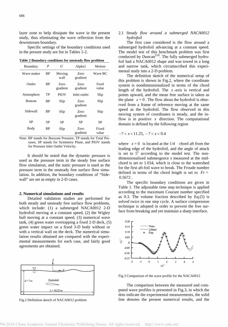
Detailed validation studies are performed for both steady and unsteady free surface flow problems, which include: (1) a submerged NACA0012 2-D hydrofoil moving at a constant speed, (2) the Wigley hull moving at a constant speed, (3) numerical wave tank, (4) green water overtopping a fixed 2-D deck, (5) green water impact on a fixed 3-D body without or with a vertical wall on the deck. The numerical simu- lation results obtained are compared with the experi- mental measurements for each case, and fairly good agreements are obtained. Fig.2 Definition sketch of NACA0012 problem

2.1 Steady flow around a submerged NACA0012 hydrofoil The first case considered is the flow around a

submerged hydrofoil advancing at a constant speed. The model test of this benchmark problem was first conducted by Duncan[24]. The fully submerged hydro- foil had a NACA0012 shape and was towed in a long and narrow tank, which circumscribed this experi- mental study into a 2-D problem.

The definition sketch of the numerical setup of this problem is shown in Fig.2, where the coordinate system is nondimensionalized in terms of the chord length of the hydrofoil. The z -axis is vertical and points upward, and the mean free surface is taken as the plane = 0z . The flow about the hydrofoil is obse- rved from a frame of reference moving at the same speed as the hydrofoil. The flow observed in this moving system of coordinates is steady, and the in- flow is in positive x direction. The computational domain is defined by the following region

7 11.25, 7 0.4x z− < < − < < where = 0x is located at the 1/4 chord aft from the leading edge of the hydrofoil, and the angle of attack is set to 5o according to the model test. The non- dimensionalized submergence s measured at the mid- chord is set to 1.034, which is close to the watershed for the first aft-foil wave to break. The Froude number defined in terms of the chord length is set to =Fr 0.5672 .

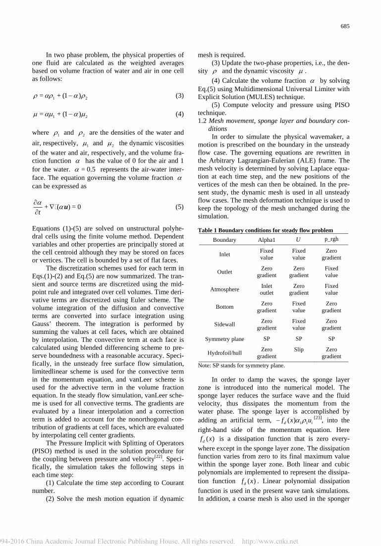
The specific boundary conditions are given in Table 1. The adjustable time step technique is applied according to the maximum Courant number specified as 0.3. The volume fraction described by Eq.(5) is solved twice in one step cycle. A surface compression technique is adopted in order to prevent the free sur- face from breaking and yet maintain a sharp interface. Fig.3 Comparison of the wave profile for the NACA0012

The comparison between the measured and com- puted wave profiles is presented in Fig.3, in which the dots indicate the experimental measurements, the solid line denotes the present numerical results, and the

687

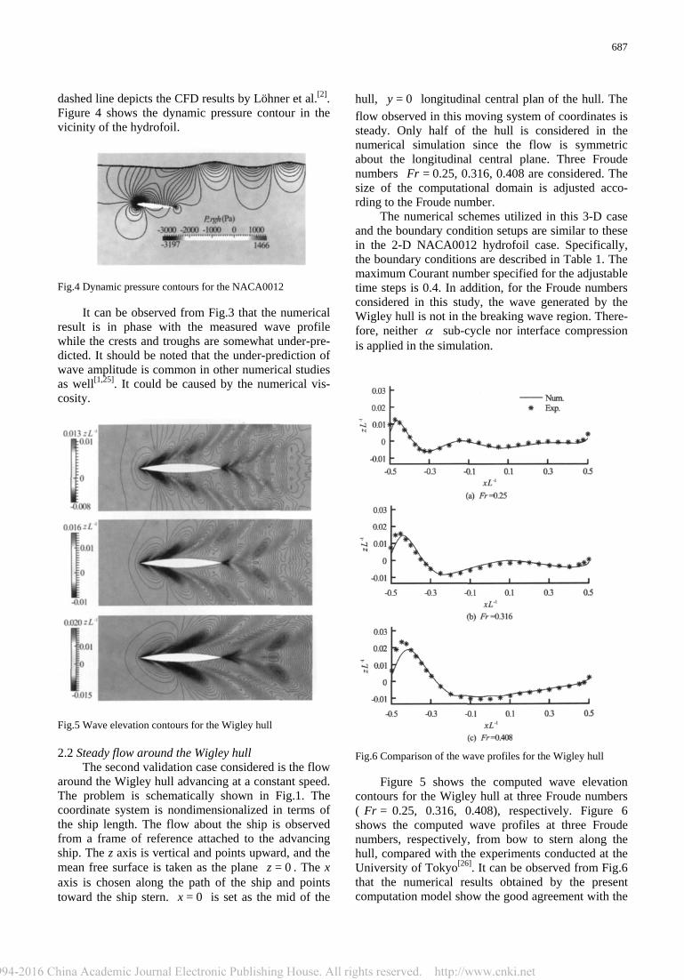
dashed line depicts the CFD results by Löhner et al.[2]. Figure 4 shows the dynamic pressure contour in the vicinity of the hydrofoil. Fig.4 Dynamic pressure contours for the NACA0012

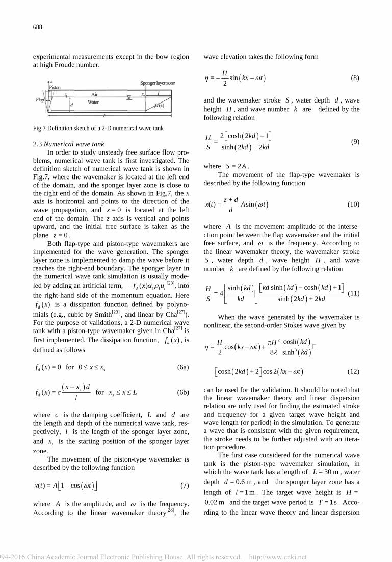
It can be observed from Fig.3 that the numerical result is in phase with the measured wave profile while the crests and troughs are somewhat under-pre- dicted. It should be noted that the under-prediction of wave amplitude is common in other numerical studies as well[1,25]. It could be caused by the numerical vis- cosity. Fig.5 Wave elevation contours for the Wigley hull 2.2 Steady flow around the Wigley hull

The second validation case considered is the flow around the Wigley hull advancing at a constant speed. The problem is schematically shown in Fig.1. The coordinate system is nondimensionalized in terms of the ship length. The flow about the ship is observed from a frame of reference attached to the advancing ship. The z axis is vertical and points upward, and the mean free surface is taken as the plane = 0z . The x axis is chosen along the path of the ship and points toward the ship stern. = 0x is set as the mid of the

hull, = 0y longitudinal central plan of the hull. The flow observed in this moving system of coordinates is steady. Only half of the hull is considered in the numerical simulation since the flow is symmetric about the longitudinal central plane. Three Froude numbers =Fr 0.25, 0.316, 0.408 are considered. The size of the computational domain is adjusted acco- rding to the Froude number.

The numerical schemes utilized in this 3-D case and the boundary condition setups are similar to these in the 2-D NACA0012 hydrofoil case. Specifically, the boundary conditions are described in Table 1. The maximum Courant number specified for the adjustable time steps is 0.4. In addition, for the Froude numbers considered in this study, the wave generated by the Wigley hull is not in the breaking wave region. There- fore, neither α sub-cycle nor interface compression is applied in the simulation. Fig.6 Comparison of the wave profiles for the Wigley hull

Figure 5 shows the computed wave elevation contours for the Wigley hull at three Froude numbers ( =Fr 0.25, 0.316, 0.408), respectively. Figure 6 shows the computed wave profiles at three Froude numbers, respectively, from bow to stern along the hull, compared with the experiments conducted at the University of Tokyo[26]. It can be observed from Fig.6 that the numerical results obtained by the present computation model show the good agreement with the

688

experimental measurements except in the bow region at high Froude number. Fig.7 Definition sketch of a 2-D numerical wave tank 2.3 Numerical wave tank

In order to study unsteady free surface flow pro- blems, numerical wave tank is first investigated. The definition sketch of numerical wave tank is shown in Fig.7, where the wavemaker is located at the left end of the domain, and the sponger layer zone is close to the right end of the domain. As shown in Fig.7, the x axis is horizontal and points to the direction of the wave propagation, and = 0x is located at the left end of the domain. The z axis is vertical and points upward, and the initial free surface is taken as the plane = 0z .

Both flap-type and piston-type wavemakers are implemented for the wave generation. The sponger layer zone is implemented to damp the wave before it reaches the right-end boundary. The sponger layer in the numerical wave tank simulation is usually mode- led by adding an artificial term, 1 1( )d if x uα ρ− [23], into the right-hand side of the momentum equation. Here

( )df x is a dissipation function defined by polyno- mials (e.g., cubic by Smith[23] , and linear by Cha[27]). For the purpose of validations, a 2-D numerical wave tank with a piston-type wavemaker given in Cha[27] is first implemented. The dissipation function, ( )df x , is defined as follows

( ) = 0df x for 0 sx x≤ ≤ (6a)

( )( ) = s

d

x x df x c

l−

for sx x L≤ ≤ (6b)

where c is the damping coefficient, L and d are the length and depth of the numerical wave tank, res- pectively, l is the length of the sponger layer zone, and sx is the starting position of the sponger layer zone.

The movement of the piston-type wavemaker is described by the following function

( )( ) = 1 cosx t A tω−⎡ ⎤⎣ ⎦ (7) where A is the amplitude, and ω is the frequency. According to the linear wavemaker theory[28], the

wave elevation takes the following form

( )= sin2H kx tη ω− − (8)

and the wavemaker stroke S , water depth d , wave height H , and wave number k are defined by the following relation

( )( )

2 cosh 2 1=

sinh 2 + 2kdH

S kd kd−⎡ ⎤⎣ ⎦ (9)

where = 2S A .

The movement of the flap-type wavemaker is described by the following function

( )+( ) = sinz dx t A td

ω (10)

where A is the movement amplitude of the interse- ction point between the flap wavemaker and the initial free surface, and ω is the frequency. According to the linear wavemaker theory, the wavemaker stroke S , water depth d , wave height H , and wave number k are defined by the following relation

( ) ( ) ( )( )

sinh cosh + 1sinh= 4

sinh 2 + 2kd kd kdkdH

S kd kd kd−⎡ ⎤⎡ ⎤ ⎣ ⎦

⎢ ⎥⎣ ⎦

(11)

When the wave generated by the wavemaker is

nonlinear, the second-order Stokes wave given by

( ) ( )( )

2

3

cosh= cos

2 8 sinhkdH Hkx tkd

η ωλ

π− +

( ) ( )cosh 2 + 2 cos 2kd kx tω−⎡ ⎤⎣ ⎦ (12) can be used for the validation. It should be noted that the linear wavemaker theory and linear dispersion relation are only used for finding the estimated stroke and frequency for a given target wave height and wave length (or period) in the simulation. To generate a wave that is consistent with the given requirement, the stroke needs to be further adjusted with an itera- tion procedure.

The first case considered for the numerical wave tank is the piston-type wavemaker simulation, in which the wave tank has a length of = 30 mL , water depth = 0.6 md , and the sponger layer zone has a length of = 1 ml . The target wave height is =H

0.02 m and the target wave period is = 1sT . Acco- rding to the linear wave theory and linear dispersion

689

relation, the amplitude of the wavemaker movement is set as = 0.0054 mA . In order to validate wave ele- vations, three wave gages are placed at = , 5 ,x λ λ

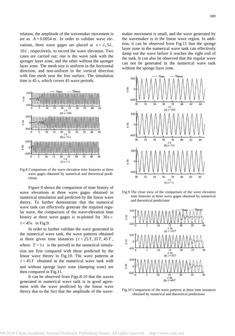
10λ , respectively, to record the wave elevation. Two cases are carried out: one is the wave tank with the sponger layer zone, and the other without the sponger layer zone. The mesh size is uniform in the horizontal direction, and non-uniform in the vertical direction with fine mesh near the free surface. The simulation time is 45 s, which covers 45 wave periods. Fig.8 Comparison of the wave elevation time histories at three

wave gages obtained by numerical and theoretical predi- ctions

Figure 8 shows the comparison of time history of

wave elevations at three wave gages obtained in numerical simulation and predicted by the linear wave theory. To further demonstrate that the numerical wave tank can effectively generate the required regu- lar wave, the comparison of the wave-elevation time history at three wave gages is re-plotted for 30s <

45st < in Fig.9. In order to further validate the wave generated in

the numerical wave tank, the wave patterns obtained at three given time instances ( = 25 , 35 , 45t T T T , where = 1sT is the period) in the numerical simula- tion are first compared with these predicted by the linear wave theory in Fig.10. The wave patterns at

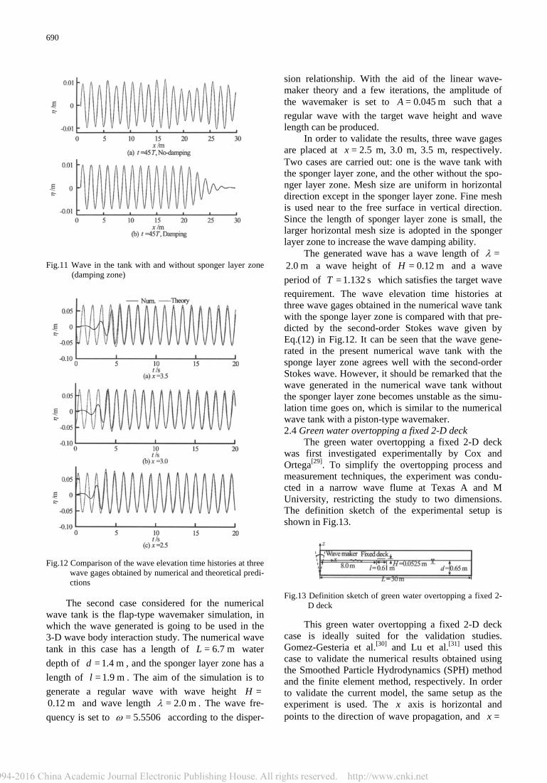
= 45t T obtained in the numerical wave tank with and without sponge layer zone (damping zone) are then compared in Fig.11.

It can be observed from Figs.8-10 that the waves generated in numerical wave tank is in good agree- ment with the wave predicted by the linear wave theory due to the fact that the amplitude of the wave-

maker movement is small, and the wave generated by the wavemaker is in the linear wave region. In addi- tion, it can be observed from Fig.11 that the sponge layer zone in the numerical wave tank can effectively damp out the wave before it reaches the right end of the tank. It can also be observed that the regular wave can not be generated in the numerical wave tank without the sponge layer zone. Fig.9 The close view of the comparison of the wave elevation

time histories at three wave gages obtained by numerical and theoretical predictions

Fig.10 Comparison of the wave patterns at three time instances

obtained by numerical and theoretical predictions

690

Fig.11 Wave in the tank with and without sponger layer zone

(damping zone) Fig.12 Comparison of the wave elevation time histories at three

wave gages obtained by numerical and theoretical predi- ctions

The second case considered for the numerical

wave tank is the flap-type wavemaker simulation, in which the wave generated is going to be used in the 3-D wave body interaction study. The numerical wave tank in this case has a length of = 6.7 mL water depth of = 1.4 md , and the sponger layer zone has a length of = 1.9 ml . The aim of the simulation is to generate a regular wave with wave height =H 0.12 m and wave length = 2.0 mλ . The wave fre- quency is set to = 5.5506ω according to the disper-

sion relationship. With the aid of the linear wave- maker theory and a few iterations, the amplitude of the wavemaker is set to = 0.045 mA such that a regular wave with the target wave height and wave length can be produced.

In order to validate the results, three wave gages are placed at =x 2.5 m, 3.0 m, 3.5 m, respectively. Two cases are carried out: one is the wave tank with the sponger layer zone, and the other without the spo- nger layer zone. Mesh size are uniform in horizontal direction except in the sponger layer zone. Fine mesh is used near to the free surface in vertical direction. Since the length of sponger layer zone is small, the larger horizontal mesh size is adopted in the sponger layer zone to increase the wave damping ability.

The generated wave has a wave length of =λ 2.0 m a wave height of = 0.12 mH and a wave period of = 1.132 sT which satisfies the target wave requirement. The wave elevation time histories at three wave gages obtained in the numerical wave tank with the sponge layer zone is compared with that pre- dicted by the second-order Stokes wave given by Eq.(12) in Fig.12. It can be seen that the wave gene- rated in the present numerical wave tank with the sponge layer zone agrees well with the second-order Stokes wave. However, it should be remarked that the wave generated in the numerical wave tank without the sponger layer zone becomes unstable as the simu- lation time goes on, which is similar to the numerical wave tank with a piston-type wavemaker. 2.4 Green water overtopping a fixed 2-D deck

The green water overtopping a fixed 2-D deck was first investigated experimentally by Cox and Ortega[29]. To simplify the overtopping process and measurement techniques, the experiment was condu- cted in a narrow wave flume at Texas A and M University, restricting the study to two dimensions. The definition sketch of the experimental setup is shown in Fig.13. Fig.13 Definition sketch of green water overtopping a fixed 2-

D deck

This green water overtopping a fixed 2-D deck case is ideally suited for the validation studies. Gomez-Gesteria et al.[30] and Lu et al.[31] used this case to validate the numerical results obtained using the Smoothed Particle Hydrodynamics (SPH) method and the finite element method, respectively. In order to validate the current model, the same setup as the experiment is used. The x axis is horizontal and points to the direction of wave propagation, and =x

691

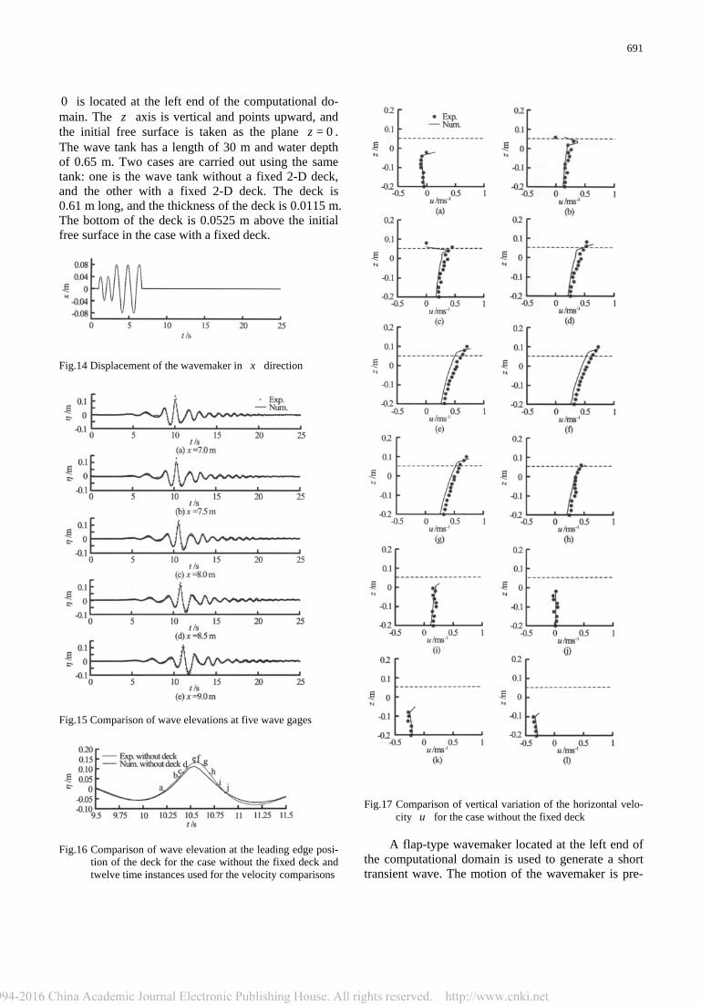
0 is located at the left end of the computational do- main. The z axis is vertical and points upward, and the initial free surface is taken as the plane = 0z . The wave tank has a length of 30 m and water depth of 0.65 m. Two cases are carried out using the same tank: one is the wave tank without a fixed 2-D deck, and the other with a fixed 2-D deck. The deck is 0.61 m long, and the thickness of the deck is 0.0115 m. The bottom of the deck is 0.0525 m above the initial free surface in the case with a fixed deck. Fig.14 Displacement of the wavemaker in x direction Fig.15 Comparison of wave elevations at five wave gages Fig.16 Comparison of wave elevation at the leading edge posi-

tion of the deck for the case without the fixed deck and twelve time instances used for the velocity comparisons

Fig.17 Comparison of vertical variation of the horizontal velo-

city u for the case without the fixed deck

A flap-type wavemaker located at the left end of the computational domain is used to generate a short transient wave. The motion of the wavemaker is pre-

692

scribed in such a way that it produces one large over- topping wave at the leading edge of the deck ( = 8 mx ) that is similar to the freak waves observed in the labo- ratory or nature. Figure 14 shows the time history of the displacement of the intersection point of the wave- maker and the initial free surface. It can be seen from Fig.14 that the wavemaker displacement comprises two cycles of a sinusoidal curve with a period of 1 =T

1.0 s and amplitude of 1 = 0.04 mA and two and a half cycles of a sinusoidal curve with a period of

2 = 1.5 sT and amplitude 2 = 0.08 mA The details of the displacement expressions can be found in Ref.[31].

It should be noted that, due to the lack of com- plete experimental data, the amplitudes of the wave- maker movement in the numerical simulations are based on the wave calibration tests. In order to cali- brate the generated overtopping wave, the time histo- ries of the wave elevations taken at five wave gages in the numerical simulation are compared with these in the experimental measurements in Fig.15 after a shift of 0.62 s in time to account for the difference of the starting time of the wavemaker between the numerical wave tank and the experimental wave tank. The dis- tance between two neighboring wave gages is =xΔ

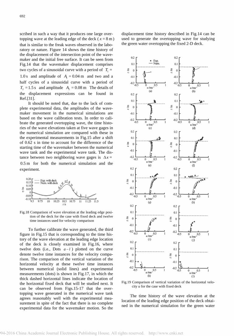
0.5 m for both the numerical simulation and the experiment. Fig.18 Comparison of wave elevation at the leading edge posi-

tion of the deck for the case with fixed deck and twelve time instances used for velocity comparison

To further calibrate the wave generated, the third

figure in Fig.15 that is corresponding to the time his- tory of the wave elevation at the leading edge location of the deck is closely examined in Fig.16, where twelve dots (i.e., Dots a l− ) plotted on the curve denote twelve time instances for the velocity compa- rison. The comparison of the vertical variation of the horizontal velocity at these twelve time instances between numerical (solid lines) and experimental measurements (dots) is shown in Fig.17, in which the thick dashed horizontal lines indicate the location of the horizontal fixed deck that will be studied next. It can be observed from Figs.15-17 that the over- topping wave generated in the numerical wave tank agrees reasonably well with the experimental mea- surement in spite of the fact that there is no complete experimental data for the wavemaker motion. So the

displacement time history described in Fig.14 can be used to generate the overtopping wave for studying the green water overtopping the fixed 2-D deck. Fig.19 Comparison of vertical variation of the horizontal velo-

city u for the case with fixed deck

The time history of the wave elevation at the location of the leading edge position of the deck obtai- ned in the numerical simulation for the green water

693

overtopping the fixed deck case is compared with the corresponding experimental measurements in Fig.18, where twelve dots (i.e., Dots a l− ) plotted on the curve denote the twelve time instances for the compa- rison of the velocity as well. The comparison of the vertical variation of the horizontal velocity at these twelve time instances between numerical simulation (solid lines) and experimental measurements (dots) is shown in Fig.19, in which the thick dashed horizontal lines indicate the location of the fixed deck. It can be seen from Figs.18 and 19 that the largest wave and its dynamics at the leading edge position of the fix deck is modeled with a reasonable accuracy for the green water overtopping the fixed deck case in comparison with the experimental measurements. It can also be observed that the effect of the deck is captured with a reasonable accuracy as well. Table 3 Dimensions of the rectangular body

Length (m) 0.4

Breadth (m) 0.52

Depth (m) 0.4

Draft (m) 0.37

Free board (m) 0.03

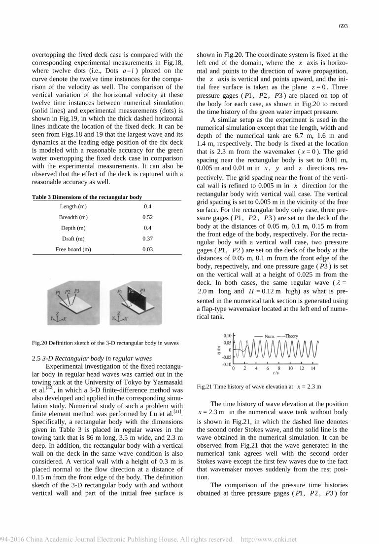
Fig.20 Definition sketch of the 3-D rectangular body in waves 2.5 3-D Rectangular body in regular waves

Experimental investigation of the fixed rectangu- lar body in regular head waves was carried out in the towing tank at the University of Tokyo by Yasmasaki et al.[32], in which a 3-D finite-difference method was also developed and applied in the corresponding simu- lation study. Numerical study of such a problem with finite element method was performed by Lu et al.[31]. Specifically, a rectangular body with the dimensions given in Table 3 is placed in regular waves in the towing tank that is 86 m long, 3.5 m wide, and 2.3 m deep. In addition, the rectangular body with a vertical wall on the deck in the same wave condition is also considered. A vertical wall with a height of 0.3 m is placed normal to the flow direction at a distance of 0.15 m from the front edge of the body. The definition sketch of the 3-D rectangular body with and without vertical wall and part of the initial free surface is

shown in Fig.20. The coordinate system is fixed at the left end of the domain, where the x axis is horizo- ntal and points to the direction of wave propagation, the z axis is vertical and points upward, and the ini- tial free surface is taken as the plane = 0z . Three pressure gages ( 1P , 2P , 3P ) are placed on top of the body for each case, as shown in Fig.20 to record the time history of the green water impact pressure.

A similar setup as the experiment is used in the numerical simulation except that the length, width and depth of the numerical tank are 6.7 m, 1.6 m and 1.4 m, respectively. The body is fixed at the location that is 2.3 m from the wavemaker ( = 0x ). The grid spacing near the rectangular body is set to 0.01 m, 0.005 m and 0.01 m in x , y and z directions, res- pectively. The grid spacing near the front of the verti- cal wall is refined to 0.005 m in x direction for the rectangular body with vertical wall case. The vertical grid spacing is set to 0.005 m in the vicinity of the free surface. For the rectangular body only case, three pre- ssure gages ( 1P , 2P , 3P ) are set on the deck of the body at the distances of 0.05 m, 0.1 m, 0.15 m from the front edge of the body, respectively. For the recta- ngular body with a vertical wall case, two pressure gages ( 1P , 2P ) are set on the deck of the body at the distances of 0.05 m, 0.1 m from the front edge of the body, respectively, and one pressure gage ( 3P ) is set on the vertical wall at a height of 0.025 m from the deck. In both cases, the same regular wave ( =λ 2.0 m long and = 0.12 mH high) as what is pre- sented in the numerical tank section is generated using a flap-type wavemaker located at the left end of nume- rical tank. Fig.21 Time history of wave elevation at = 2.3 mx

The time history of wave elevation at the position = 2.3 mx in the numerical wave tank without body

is shown in Fig.21, in which the dashed line denotes the second order Stokes wave, and the solid line is the wave obtained in the numerical simulation. It can be observed from Fig.21 that the wave generated in the numerical tank agrees well with the second order Stokes wave except the first few waves due to the fact that wavemaker moves suddenly from the rest posi- tion.

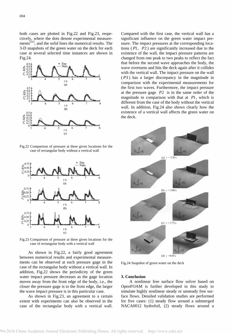
The comparison of the pressure time histories obtained at three pressure gages ( 1P , 2P , 3P ) for

694

both cases are plotted in Fig.22 and Fig.23, respe- ctively, where the dots denote experimental measure- ments[31], and the solid lines the numerical results. The 3-D snapshots of the green water on the deck for each case at several selected time instances are shown in Fig.24. Fig.22 Comparison of pressure at three given locations for the

case of rectangular body without a vertical wall Fig.23 Comparison of pressure at three given locations for the

case of rectangular body with a vertical wall

As shown in Fig.22, a fairly good agreement between numerical results and experimental measure- ments can be observed at each pressure gage in the case of the rectangular body without a vertical wall. In addition, Fig.22 shows the periodicity of the green water impact pressure decreases as the gage location moves away from the front edge of the body, i.e., the closer the pressure gage is to the front edge, the larger the wave impact pressure is in this particular case.

As shown in Fig.23, an agreement to a certain extent with experiments can also be observed in the case of the rectangular body with a vertical wall.

Compared with the first case, the vertical wall has a significant influence on the green water impact pre- ssure. The impact pressures at the corresponding loca- tions ( 1P , 2P ) are significantly increased due to the existence of the wall, the impact pressure patterns are changed from one peak to two peaks to reflect the fact that before the second wave approaches the body, the wave overturns and hits the deck again after it collides with the vertical wall. The impact pressure on the wall ( 3P ) has a larger discrepancy in the magnitude in comparison with the experimental measurements for the first two waves. Furthermore, the impact pressure at the pressure gage 2P is in the same order of the magnitude in comparison with that at 1P , which is different from the case of the body without the vertical wall. In addition, Fig.24 also shows clearly how the existence of a vertical wall affects the green water on the deck. Fig.24 Snapshot of green water on the deck 3. Conclusion

A nonlinear free surface flow solver based on OpenFOAM is further developed in this study to simulate highly nonlinear steady or unsteady free sur- face flows. Detailed validation studies are performed for five cases: (1) steady flow around a submerged NACA0012 hydrofoil, (2) steady flows around a

695

Wigley hull model, (3) numerical wave tank, (4) green water overtopping a fixed 2-D deck, (5) green water impact on a fixed 3-D body without or with a vertical wall on the deck. The numerical results obtained have been compared with the experimental measurements and other CFD results, and the agreements are satisfa- ctory. The present numerical model can thus be used to simulate highly nonlinear steady and unsteady free surface flows with reasonable accuracy. Acknowledgements

This work was partially sponsored by the Office of Naval Research, Ms. Kelly Cooper was the tech- nical monitor. The support of Program for Professor of Special Appointment (Eastern Scholar) at Shanghai Institutions of Higher Learning for this work is also gratefully acknowledged. The authors also gratefully acknowledge Dr. Cox’s kindness for sharing the experimental data for the green water overtopping a fixed 2-D deck case. References [1] HINO T., MARTINELLI L. and JAMESON A. A finite-

volume method with unstructured grid for free surface flow simulations[C]. Proc. 6th Int. Conf. on Num. Ship Hydro. Iowa City, IA, USA, 1993, 173-194.

[2] LÖHNER R., YANG C. and OÑATE E. et al. An un- structured grid based, parallel free surface solver[J]. App. Num. Math., 1999, 31(3): 271-293.

[3] YANG C., LÖHNER R. Calculation of ship sinkage and trim using a finite element method and unstructured grids[J]. Int. J. Comp. Fluid Dynamics, 2002, 16(3): 217-227.

[4] CHEN G., KHARIF C. Two-dimensional Navier-Stokes simulation of breaking waves[J]. Phys. Fluids, 1999, 11(1): 121-133.

[5] BIAUSSER B., FRAUNIE P. and GRILLI S. et al. Numerical analysis of the internal kinematics and dyna- mics of three dimensional breaking waves on slopes[J]. Int. J. of Offshore and Polar Eng., 2004, 14(4): 247- 256.

[6] LANDRINI M., COLAGOROSSI A. and FALTISEN O. M. Sloshing in 2-D flows by the SPH method[C]. Proc. 8th Int. Conf. on Num. Ship Hydro. Busan, Korea, 2003.

[7] RHEE S. H. Unstructured grid based Reynolds-Avera- ged Navier-Stokes method for liquid tank sloshing[J]. Journal of Fluids Engineering, 2005, 127(3): 572-582.

[8] YANG C., LÖHNER R. Computation of 3D flows with violent free surface motion[C]. Proc. 15th Int. Off- shore and Polar Eng. Conf., ISOPE. Seoul, Korea, 2005.

[9] FEKKEN G., VELDMAN A. E. P. and BUCHNER B. Simulation of green water loading using the Navier- Stokes equations[C]. Proc. 7th Int. Conf. Num. Ship Hydro. Nantes, France, 1999.

[10] HUIJSMANS R. H. M., VAN GROSEN E. Coupling freak wave effects with green water simulations[C]. Proc. 14th Int. Offshore and Polar Eng. Conf.,

ISOPE. Toulon, France, 2004. [11] GRECO M., LANDRINI M. and FALTINSEN O. M.

Impact flows and loads on ship-deck structures[J]. Journal of Fluids Structures, 2004, 19(3): 251-275.

[12] YANG C., LU H. and LÖHNER R. et al. Numerical simulation of highly nonlinear wave-body interactions with experimental validation[C]. Proc. of Int. Conf. Violent Flows (VF-2007). Fukuoka, Japan, 2007.

[13] LU H., YANG C. and LÖHNER R. Numerical studies of ship-ship interactions in extreme waves[C]. Proc. Grand Challenges in Modeling and Simulations (GCMS’09). Istanbul, Turkey, 2009, 1: 43-55.

[14] SHIBATA K., KOSHIZUKA S. Numerical analysis of shipping water impact on a deck using a particle method[J]. Ocean Eng., 2007, 34(3-4): 585-593.

[15] HU C., KASHIWAGI M. Numerical and experimental studies on three-dimensional water on deck with a modified Wigley model[C]. Proc. 9th Int. Conf. Num. Hydro. Michigan, USA, 2007, 1: 159-169.

[16] HU C., SUEYOSHI M. and KASHIWAGI M. Nume- rical simulation of strongly nonlinear wave-ship intera- ction by CIP based Cartesian grid method[J]. Int. J. of Offshore and Polar Eng., 2010, 20(2): 81-87.

[17] LÖHNER R., YANG C. and OÑATE E. On the simu- lation of flows with violent free surface motion[J]. Comp. Methods in Appl. Mech. and Eng., 2006, 195(41-43): 5597-5620.

[18] LÖHNER R., YANG C. and OÑATE E. Simulation of flows with violent free surface motion and moving objects using unstructured grids[J]. Int. J. for Num. Methods in Fluids, 2007, 53(8): 1315-1338.

[19] YANG C., LÖHNER R. On the modeling of highly nonlinear wave-body interactions[C]. Proc. 16th Int. Offshore and Polar Eng. Conf., ISOPE. San Francisco, USA, 2006.

[20] YANG C., LÖHNER R. and LU H. An unstructured- grid based volume-of-fluid method for extreme wave and freely-floating structure interaction[C]. Proc. Conf. Global Chinese Scholars on Hydrodynamics. Shanghai, 2006, 415-422.

[21] YANG C., LU H. and LÖHNER R. et al. An unstru- ctured-grid based VOF method for ship motions indu- ced by extreme waves[C]. 9th Int. Conf. Num. Ship Hydro. Ann Arbor, USA, 2007.

[22] ISSA R. I. Solution of the implicitly discretised fluid flow equations by operator-splitting[J]. J. Comp. Phys., 1986, 62(1): 40-65.

[23] SMITH R. K. Computation of viscous multiphase hydrodynamics and ship motions during wave-slap events and wave excited roll[D]. Master Thesis, USA: The Pennsylvania State University, 2009.

[24] DUNCAN J. H. The breaking and non-breaking wave resistance of a two-dimensional hydrofoil[J]. J. Fluid Mech., 1983, 126: 507-520.

[25] RHEE S. H., STERN F. RANS model for spilling brea- king waves[J]. J. of fluids Eng., 2002, 124(2): 424-432.

[26] ITTC Cooperative experiments on Wigley parabolic model in Japan[C]. 17th ITTC Resistance Committee Report. 1983.

[27] CHA Jing-jing. Numerical wave generation and abso- rption based on OpenFOAM[D]. Master Thesis, Shanghai: Shanghai Jiao Tong University, 2011(in Chinese).

[28] DEAN R. G., DALRYMPLE R. A. Water wave mechanics for engineers and scientists[M]. Singapore: World Scientific Pub., 1991.

696

[29] COX D. T., ORTEGA J. A. Laboratory observation of green water overtopping a fixed deck[J]. Ocean Engi- neering, 2001, 29(14): 1827-1840.

[30] GOMEZ-GESTEIRA M., CERQUEIRO D. and CRESPO C. et al. Green water overtopping analyzed with a SPH model[J]. Ocean Engineering, 2005, 32(2): 223-238.

[31] LU H., YANG C. and LÖHNER R. Numerical studies of green water impact on fixed and moving bodies[C]. Proc. 20th Int. Offshore and Polar Eng. Conf., ISOPE, Beijing, 2010.

[32] YAMASAKI J., MIYATA H. and KANAI A. Finite- difference simulation of green water impact on fixed and moving bodies[J]. J. Mar. Sci. Technol., 2005, 10(1): 1-10.