Open Research OnlineThe Open University’s repository of research publicationsand other research outputs

Numerical simulations of granular dynamics II: Particledynamics in a shaken granular materialJournal ItemHow to cite:

Murdoch, Naomi; Michel, Patrick; Richardson, Derek C.; Nordstrom, Kerstin; Berardi, Christian R.; Green,Simon F. and Losert, Wolfgang (2012). Numerical simulations of granular dynamics II: Particle dynamics in a shakengranular material. Icarus, 219(1) pp. 321–335.

For guidance on citations see FAQs.

c© 2012 Elsevier Inc.

Version: Accepted Manuscript

Link(s) to article on publisher’s website:http://dx.doi.org/doi:10.1016/j.icarus.2012.03.006

Copyright and Moral Rights for the articles on this site are retained by the individual authors and/or other copyrightowners. For more information on Open Research Online’s data policy on reuse of materials please consult the policiespage.

oro.open.ac.uk

Murdoch et al.

1

1

Numerical simulations of granular dynamics II. Particle dynamics in

a shaken granular material

Naomi Murdoch†*

Patrick Michel*

Derek C. Richardson!

Kerstin Nordstrom"

Christian R. Berardi"

Simon F. Green†

Wolfgang Losert"

† The Open University

PSSRI, Walton Hall

Milton Keynes, MK7 6AA, UK

* University of Nice Sophia Antipolis, CNRS

Observatoire de la Côte d’Azur, B.P. 4229

06304 Nice Cedex 4, France

! Department of Astronomy, University of Maryland,

College Park MD 20742-2421, USA

" Department of Physics/IPST/IREAP, University of Maryland,

College Park MD 20742-2421, USA

Murdoch et al.

2

2

Printed March 1, 2012

Submitted to Icarus

78 manuscript pages

5 tables

12 figures including 1 in colour (online version only)

Murdoch et al.

3

3

Proposed running page head: Numerical simulations of shaken granular material

Please address all editorial correspondence and proofs to:

Naomi Murdoch

Laboratoire Lagrange (UMR 7293)

Observatoire de la Côte d’Azur

B.P. 4229

06304 Nice Cedex 4

France

Tel: +33 4 9200 1957

Fax: +33 4 9200 3058

E-mail: murdoch@oca.eu

Abstract

Surfaces of planets and small bodies of our Solar System are often covered by a layer

of granular material that can range from a fine regolith to a gravel-like structure of

varying depths. Therefore, the dynamics of granular materials are involved in many

events occurring during planetary and small-body evolution thus contributing to their

geological properties.

We demonstrate that the new adaptation of the parallel N-body hard-sphere code

pkdgrav has the capability to model accurately the key features of the collective

motion of bidisperse granular materials in a dense regime as a result of shaking. As a

stringent test of the numerical code we investigate the complex collective ordering

and motion of granular material by direct comparison with laboratory experiments.

We demonstrate that, as experimentally observed, the scale of the collective motion

increases with increasing small-particle additive concentration.

We then extend our investigations to assess how self-gravity and external gravity

affect collective motion. In our reduced-gravity simulations both the gravitational

conditions and the frequency of the vibrations roughly match the conditions on

asteroids subjected to seismic shaking, though real regolith is likely to be much more

heterogeneous and less ordered than in our idealised simulations. We also show that

collective motion can occur in a granular material under a wide range of inter-particle

gravity conditions and in the absence of an external gravitational field. These

investigations demonstrate the great interest of being able to simulate conditions that

are to relevant planetary science yet unreachable by Earth-based laboratory

experiments.

Murdoch et al.

5

5

Keywords: Asteroids, surfaces; Collisional physics; Geological processes;

Regoliths; Experimental techniques

Murdoch et al.

6

6

1. INTRODUCTION

Surfaces of planets and small bodies of our Solar System are often covered by a layer

of granular material that can range from a fine regolith to a gravel-like structure of

varying depths. Therefore, the dynamics of granular materials are involved in many

events occurring during planetary and small-body evolution thus contributing to their

geological properties.

The existence of granular material covering small bodies (asteroids, comets) was

inferred from thermal infrared observations that indicate that asteroids, even small and

fast rotating ones, generally have low thermal inertias compared to bare rock (Delbo

and Tanga, 2009 and references therein). This granular material has also been directly

observed by the two space missions that performed detailed characterizations of two

near-Earth asteroids (NEAs): the NEAR-Shoemaker probe (NASA) that orbited the

30 km-size asteroid Eros for one year during 2000–2001 (Cheng et al. 2002) and the

Hayabusa probe (JAXA) that visited the 500-m size asteroid Itokawa for 3 months in

2005 and successfully returned a sample from its surface to Earth in June 2010

(Tsuchiyama et al. 2011). In both cases, a layer of regolith covers the surface,

although the properties of this regolith vary greatly from one object to the other. On

Eros the regolith consists of fine dust of an estimated depth between 10 to 100 meters

(Veverka et al. 2000). On Itokawa the regolith consists of gravel and pebbles larger

than one millimeter with a depth that is probably not greater than one meter

(Miyamoto et al. 2007). The reason for these different properties is not clearly

understood, but we note that because of their size (mass) difference, if gravity is the

discriminator, then Itokawa is expected to be as different from Eros, geologically, as

Eros is from the Moon (Asphaug 2009). However, the gravity in both cases is low

Murdoch et al.

7

7

enough for processes such as seismic shaking to lead potentially to long-range surface

motion and modification.

Seismic shaking is expected to occur when small projectiles impact the surface of

small bodies on which gravity is low enough that surface motion can be influenced

over long distances by seismic wave propagation. As a result of the seismic shaking,

the surface granular material can be subject to various kinds of motion, among them,

downslope migration and degradation, or motion leading to the erasure of small

craters. Characterizing such motion under different conditions should allow us both to

better assess surface evolution and to interpret observed features. For instance, there is

an observed paucity of small craters on both Eros and Itokawa. Impact-induced

seismic shaking, which causes the regolith to move, may erase small crater features

and thus explain their paucity compared to predictions of dynamical models of

projectile populations (see e.g., Richardson et al. 2004, Michel et al. 2009). The

location and morphology of gravel on Itokawa indicate that the small body has

experienced considerable shaking. This shaking triggered global-scale granular

processes in the dry, vacuum, microgravity environment. These processes likely

include landslide-like granular migration and particle sorting, which result in the

segregation of fine gravels into areas of gravitational potential lows (Miyamoto et al.

2007).

Understanding the response of granular media to a variety of stresses is also important

in the design of sampling tools for deployment on planetary and small-body surfaces,

since the efficiency of collecting a sample from the surface of such bodies is highly

dependent on its surface properties. Sample-return missions to asteroids have been

Murdoch et al.

8

8

studied by at least three main space agencies: ESA, JAXA (who have performed the

first ever successful asteroid sample return mission) and NASA. Studies of sampling

tool design generally assume that the surfaces consist of granular materials;

consequently in-depth knowledge of their response to various stresses is required.

While constitutive equations linking stress and strain are empirically known for most

granular interactions on Earth, they involve a wide range of forces from gravity to air-

grain coupling to liquid bridges due to humidity, to electrostatic effects, to surface

shape and chemistry-dependent van der Waals forces. However, the inferred scaling

of these equations to the gravitational and environmental conditions on other

planetary bodies such as asteroids, as discussed in Scheeres et al. (2010), is currently

untested.

This need to better understand granular interaction on disparate planetary bodies

motivated us to conduct numerical simulations of granular material dynamics.

Various numerical codes have been developed to study granular dynamics (Mehta

2007). Some of these codes are purely hydrodynamic in the sense that the granular

material is represented as a fluid or as a continuum (e.g., Elaskar et al. 2000).

However, the homogenization of the granular-scale physics is not necessarily

appropriate and in most cases the discreteness of the particles and the forces between

particles (and walls) need to be taken into account (Wada et al. 2006). Other codes,

such as soft- and hard-sphere molecular dynamics codes, or codes using the Discrete

Element Method (DEM) have also been developed, all of which treat the granular

material as interacting solid particles (Cleary and Sawley 2002; Fraige et al. 2008;

Latham et al. 2008; Szarf et al. 2011; Hong and McLennan 1992; Huilin et al. 2007;

Kosinski and Hoffman 2009).

Murdoch et al.

9

9

There have been several recent contributions focussing on rubble piles (defined in

Richardson et al. (2002) as a special case of a gravitational aggregate) that have

further highlighted the connection between granular physics and planetary science.

Specifically, Walsh et al. (2008) perform hard-sphere numerical simulations to show

that binary asteroids may be created by the slow spin-up of a rubble pile asteroid by

means of the thermal YORP (Yarkovsky–O'Keefe–Radzievskii–Paddack) effect. The

properties of binaries produced by their model match those currently observed in the

small near-Earth and main-belt asteroid populations, including 1999 KW4. Goldreich

and Sari (2009) develop a quantitative theory for the effective dimensionless rigidity

of a self-gravitating rubble pile and then use this theory to investigate the tidal

evolution of rubble pile asteroids. Additionally, Sanchez and Scheeres (2011)

simulate the mechanics of asteroid rubble piles using a self-gravitating soft-sphere

Distinct Element Method model. One important mechanical property of such rubble

piles, which is not directly included in the models, is fragility. The fragility

characterises whether the material will deform in a brittle or ductile way and this may

strongly influence the evolution of small bodies under external forcing.

In this paper, we employ the N-body hard-sphere discrete element code pkdgrav

(Stadel 2001), which has been adapted to enable dynamic modelling of granular

materials in the presence of a variety of boundary conditions (Richardson et al. 2011;

hereafter Paper I). Whereas the soft-sphere methods produce contact forces by relying

upon modest penetration between particles, the hard-sphere method resolves

collisions by anticipating trajectory crossing. This provides hard-sphere codes with a

major time advantage in the resolution of a single collision; what requires dozens of

Murdoch et al.

10

10

time-steps for a soft-sphere code is resolved by hard-sphere codes in a single

calculation. However, both methods have their respective strengths; the hard-sphere

method permits longer time-steps in the dilute regime and requires fewer material

parameters, while the soft-sphere method enables more realistic treatment of friction,

and is better suited to true parallelism (Schwartz et al., 2011). The advantages of the

N-body hard-sphere adaptation of pkdgrav over many other hard and soft discrete

element approaches include full support for parallel computation and a unique

combination of the use of hierarchical tree methods to rapidly compute long-range

inter-particle forces (namely gravity, when included) and to locate nearest neighbours

and potential colliders (which then interact via the hard sphere potential). In addition,

collisions are determined prior to advancing particle positions, ensuring that no

collisions are missed and that collision circumstances are computed exactly (in

general, to within the accuracy of the integration), which is a particular advantage

when particles are moving rapidly. There are also options available for particle

bonding to make irregular shapes that are subject to Euler’s laws of rigid-body

rotation with non-central impacts (cf. Richardson et al., 2009). Our approach is

designed to be general and flexible: any number of walls can be combined in arbitrary

ways to match the desired configuration without changing any code, whereas many

existing methods are tailored for a specific geometry. Our long-term goal is to

understand how scaling laws, different flow regimes, segregation, and so on change

with gravity, and to apply this understanding to asteroid surfaces, without the need to

simulate the surfaces in their entirety. Before we can simulate granular interactions on

planetary bodies, the simulations must first be able to reproduce the dynamics of

granular materials in more idealised conditions and match the results of existing

laboratory experiments.

Murdoch et al.

11

11

Granular material dynamics is a field of intensive research with a range of industrial

applications. A variety of laboratory experiments and numerical methods have been

developed to study granular dynamics, but the applications of these experiments to

problems related to celestial body surfaces have only recently begun. For example,

Wada et al. (2006) studied the cratering process on granular materials both by impact

experiments and numerical simulations using DEM. Regolith motion resulting from

seismic shaking of asteroids has also been discussed in several papers, but without

simulating explicitly the dynamics of the regolith. For instance, Richardson et al.

(2005) investigated the global effects of seismic activity resulting from impacts on the

surface morphology of fractured asteroids. They used a Newmark slide-block analysis

(Newmark, 1965), which can be applied in the regime where the regolith layer

thickness is much smaller than the seismic wavelengths involved. In this case,

modelling the motion of a rigid block resting on an inclined plane approximates the

motion of a mobilized regolith layer. Miyamoto et al. (2007) discussed regolith

migration and sorting on the asteroid Itokawa by analyzing regolith properties from

images obtained by the Hayabusa probe and derived the possible regolith motion due

to seismic shaking based on experiments performed on Earth.

In this paper we demonstrate that despite the fact that in our numerical scheme only

two-body collisions are resolved (in comparison to the soft-sphere model where

collisions between multiple particles occur), this adaptation of pkdgrav has the

capability to accurately model the key features of the collective ordering and

collective motion of a shaken granular material in a dense regime. This special case is

suitable for the hard-sphere approach, but we recognise that, in general, dense systems

Murdoch et al.

12

12

involving multiple collisions and enduring contacts that then require a soft-sphere

approach. We have in fact implemented a soft-sphere method in our code that has

been tested against physical experiments (Schwartz et al. 2012, submitted), and are in

the process of developing a hybrid method that switches between both approaches as

needed. However, for the present purpose, the hard-sphere approach is in fact more

efficient, since, as we will demonstrate (Sec. 4), the assumption of instantaneous

single-point-contact collisions is appropriate for the shaking experiments and so larger

time-steps can be used in the simulations.

The experiment used as a reference basis of shaking motion is described in Berardi et

al. (2010). We chose this experiment as it focuses on collective behaviour where

multiple particles move in a coordinated string-like fashion. We expect this collective

motion will provide a more stringent test of the simulation than statistics of individual

particle motion. In addition, string-like dynamics are also an indicator of fragility, an

important property to consider.

We will first present the experiments that served as a reference basis for our

numerical simulations of shaking motion in Sec. 2. We briefly describe the code in

Sec. 3 (full details can be found in Paper I) and then Sec. 4 provides details on how

the numerical simulations were performed. In Sec. 5 discussions are provided about

the different analysis techniques and approaches that can be applied for such a

simulation and laboratory experiment and an in-depth discussion is included

highlighting the difficulties in comparing experimental and simulation data. A

detailed comparison (either qualitative or, where appropriate, quantitative) is

performed with the laboratory experiments. Then, in Sec. 6 we consider the

Murdoch et al.

13

13

consequences of varying gravitational acceleration on string frequency and length.

This demonstrates the ability of our code to simulate the range of gravitational

environments that can be encountered among the solid planetary bodies within our

solar system. Indeed, in our reduced-gravity simulations both the gravitational

conditions and the frequency of the vibrations roughly match the conditions on

asteroids subjected to seismic shaking (Richardson et al., 2004; 2005), though real

regolith is likely to be much more heterogeneous and less ordered than in our

idealised simulations. In this same section we also demonstrate one of the unique

abilities of our code: the ability to model inter-particle gravity. By removing the

external gravitational field and varying the particle density we examine what happens

to our granular system when the gravitational forces between the particles become

increasingly strong. Finally, in Sec. 7 we discuss the relevance of our results to

planetary science and discuss future perspectives.

2. SHAKING EXPERIMENTS

The experimental studies used as a reference in this investigation were aimed at

analyzing the motion of dense configurations of bidisperse particles under vertical

shaking (Berardi et al. 2010). The studies were carried out in a pseudo two-

dimensional system (see Fig. 1). The goal was to analyse how a system of large and

small particles arranges into ordered and disordered regions, and to elucidate the

dynamics, especially in the more mobile disordered regions. The observed structure

and dynamics show strong similarities to grains and grain boundaries, with large

particles arranging into hexagonally ordered grain-like regions and small particles

localized in grain boundaries. Additionally, the particle dynamics in the grain

Murdoch et al.

14

14

boundary are similar in character to a super-cooled fluid with string-like collective

motion. Both the ordering and string-like dynamics are collective effects. In the

experiments it was found that addition of small particles enhances the number and

length of strings. Strings and ordering can both affect how fragile the ensemble of

particles is, i.e., how suddenly the material jams or fails and flows under an

incremental strain. Therefore by simulating this laboratory experiment we can assess

the ability of the numerical code to capture collectively emerging structures and

dynamics with a focus on those collective structures and dynamics that significantly

affect the mechanical properties of the ensemble.

In the laboratory experiment steel spheres 3.0 mm in diameter (with the addition of

2.0 mm steel spheres, which take up from 3 to 10% of the covered surface area) were

confined into a dense arrangement in a round container of 292 mm diameter with 0.1

mm separation between the large particles and a covering lid (see Fig. 1 for a diagram

of the experiment and Table 1 for exact experiment conditions). When the container

was vibrated vertically (at a frequency of 125 Hz with a maximum acceleration of 4.5

g), the dense arrangement of particles moved vertically and horizontally in a way that

is characteristic for systems close to jamming. Most significantly, many of the larger

(3 mm) particles formed hexagonal close-packed arrangements (the densest possible

configuration of spheres in a plane). Such ordered regions, which we refer to as

grains, are similar to crystalline grains in polycrystalline materials. These grains are

surrounded by less densely packed, disordered regions that are named grain

boundaries. It is in these grain boundary regions that most of the smaller 2 mm

particles can be found. Particle motion was imaged with a high-speed high-resolution

camera. From the images, the position and the motion of large and small particles

Murdoch et al.

15

15

were determined using an adaptation of a subpixel-accuracy particle detection and

tracking algorithm (Crocker and Grier, 1996). First, images were bandpass filtered to

emphasize the known particle size scale. This yields well-separated bright peaks

whose positions are found with subpixel-accuracy (better than 0.13 mm) by peak-

finding algorithms. To analyse motion, peaks (i.e., particles) are then tracked through

image sequences that require that particles move less than half a particle diameter

between frames. Comparison with the original image shows that more than 99% of

all particles in each frame are detected with this algorithm. A particle track was

labelled as large or small based on the average brightness of the peak. This correctly

labels more than 99.9% of large particles and more than 96.1% of small particles.

The diffusion coefficient, D, of a system of particles has units of length-squared

over time. Thus, the characteristic timescale to diffuse over a distance L is L2/D. The

statistics of motion therefore provides a characteristic timescale when considering

motion over characteristic length-scales of a particle radius. Mobile particles then can

be identified based on their larger-than-expected displacement over this characteristic

time interval. One characteristic of mobile particles in a system close to jamming is

that mobile particles leave their “cage” of neighbours, i.e., they change neighbours.

Indeed the local geometric arrangement affects mobility - mobile particles

preferentially appear in grain boundaries. Similarly, string-like collective motion of

mobile particles is a characteristic for systems close to jamming, particularly in glassy

systems (disordered systems with extremely slow dynamics that are below and

slightly above the glass transition) and dense suspensions of colloidal particles

(Donati et al. 1998, Weeks et al. 2000). Rearrangements of mobile particles are

Murdoch et al.

16

16

characterized as strings, if particles move towards each other’s previous position as if

they were beads moving along a string.

The existence of this collective particle motion and the length and number of

cooperatively moving clusters of particles (hereafter granular strings) can be

determined (Donati et el. 1998, Aichele et al. 2003, Riggleman et al, 2006 and Zhang

et al. 2009). Berardi et al. (2010) found that the surface area occupied by grain

boundaries and the length and number of the granular strings increases with

increasing concentrations of small particles.

Both grain boundaries and granular strings are not only useful as more subtle

measures to assess whether our simulations recover collective ordering and motion,

but they also affect important materials properties. Strings highlight how the yielding

of granular matter is similar to the plasticity of glasses; both exhibit similar string-like

collective dynamics (Stevenson and Wolynes, 2010). The presence of strings indicates

that a material is fragile. In glasses, fragility is generally defined as how quickly

viscosity increases when the temperature of a material is lowered toward the glass

transition temperature. In granular matter, strain may be considered as the equivalent

of temperature (Lui and Nagel, 1998) and fragility is associated with sudden changes

in strain with increasing stress. Granular materials are, by their nature, thought to be

fragile and are, therefore, prone to sudden, avalanche-like failures (Riggleman et al.

2006).

Measurements of string length offer one way to quantify this propensity for fragile

behaviour – longer strings have been shown to indicate higher fragility (Dudowicz et

Murdoch et al.

17

17

al. 2005). In contrast, short granular strings indicate a more ductile behaviour, where

failure and granular rearrangements are more uniformly distributed in space and time.

String-like dynamics within grain boundaries directly affect grain boundary mobility

and, therefore, play an important role in the bulk mechanical properties of more

ordered systems (increased grain boundary mobility implies increased ductility)

(Zhang et al. 2006).

While previous simulations have shown that strings exist in elastic disordered systems

(Dudowicz et al. 2005) and in ordered systems with grain boundaries (Zhang 2006),

the simulation of strings in a dissipative system in general, and in a vibrated lattice in

particular has not been previously carried out. In addition, this study is the first direct

comparison of the frequency and length of granular strings between experiment and

simulation.

[FIGURE 1 GOES HERE]

[TABLE 1 GOES HERE]

3. NUMERICAL CODE

The code used for our experiments is a modified version of the cosmology code

pkdgrav (Stadel 2001) that was adapted to handle hard-body collisions (Richardson

et al. 2000). The granular dynamics modifications consist primarily of providing wall

“primitives” to simulate the boundaries of the experimental apparatus.

Implementation details are given in Paper I; only a very short summary is provided

here for reference.

Murdoch et al.

18

18

The code uses a second-order leapfrog scheme to integrate the equations of motion,

which in this case describe ballistic trajectories in a uniform gravity field. Collision

events are predicted during the linear position update portion of each integration time-

step. Collisions are carried out in time order, properly accounting for repeated

collisions between particles (and between particles and walls) during each step.

Particles are treated as rigid spheres (so the collisions are instantaneous), with

collision outcomes parameterized by coefficients of normal and tangential restitution.

In addition to having a velocity vector, each particle also has a spin vector allowing

particle rotation to be treated (if the tangential coefficient of restitution is < 1). The

full collision resolution equations are given in Paper I.

Walls are treated as having infinite mass (so they are not affected by collisions).

Paper I describes four wall primitives that can be combined in arbitrary ways: infinite

plane, finite disk, infinite cylinder, and finite cylinder (the finite primitives consist of

a surface combined with one or two thin rings). Certain primitives can have limited

translational or rotational motion. The simulations described here used combinations

of infinite planes to simulate the apparatus; two of the planes are vibrating, namely

the confining lid and base-plate (Sec. 4).

4. NUMERICAL SIMULATION METHOD

The area covered by the particles is calculated by projecting the spheres, as 2d circles,

onto the plane of the bottom of the container. The surface area coverage is then the

percentage of the total container surface area that is covered by the projected surface

area of all of the particles. We use this definition instead of the usual ‘volume

Murdoch et al.

19

19

fraction’ because we are dealing with a quasi-2d and not a full 3d system. Similarly,

the small particle surface area coverage, or small particle concentration, is defined as

the percentage of total surface area covered by the small-particle additive. In the

experiments (Berardi et al. 2010) the surface area coverage studied was 85%.

The following method was used to reach a similar total surface area coverage as in

experiments (Berardi et al. 2010). First, a box of 120 mm # 120 mm is constructed

using the infinite plane geometries now available in pkdgrav (Paper I). Four

infinite planes, two with normal vectors in the positive and negative x-directions and

two with normal vectors in the positive and negative y-directions, form the sides of

the box. One infinite plane with normal vector in the z-direction forms the base of the

box.

The monolayer of particles at the bottom of the box is created in several steps. First,

several layers of particles with radius (Rp) 1.5 mm are generated starting at a height of

approximately 15 mm (10 Rp) above the base of the box (measured from the base of

the box to the center of the particles in the bottom layer). The particles in each layer

are evenly distributed in the x and y directions with a spacing of 4.5 mm (3 Rp)

between the centers of the particles in each direction. The z position of each particle

is randomly generated within the limits of ±1/Rp from the mean layer height. This is to

prevent all particles in each layer from impacting the base of the box simultaneously,

which is unrealistic (it would be impossible in an experiment to drop all the balls from

the same height exactly simultaneously). The number of particles generated depends

on the desired final surface area coverage and small particle concentration. Due to the

fixed inter-particle spacing there are 625 particles in each generated, and dropped, full

Murdoch et al.

20

20

layer. However, in order to have the correct number of particles in the box, the last

layer dropped into the container is often a partial layer. The particle layers are formed

one at a time by generating rows of particles from one side of the box to the other.

All the particles are given a small initial velocity on the order of 1 mm s-1

in the x and

y directions but not in the vertical z direction. Gravity (acceleration in the vertical z

direction) is 1 g (where g = 9.8 m s-2

).

At the start of the simulation the generated layers of particles are allowed to fall into

the box, under gravity (with no inter-particle gravity). The simulation runs until the

mean vertical component of the particle translational velocity drops below a threshold

of 0.1 mm s-1

, i.e., the particles are in one single layer and continue to move around

the bottom of the box but are no longer bouncing in a significant way. The time-step

used for the dropping phase of the simulations is such that for a particle starting from

rest and falling under gravity it would take approximately 30 time-steps for it to drop

one particle diameter.

A fraction of large particles are then replaced with smaller ones (radius 1 mm). In

these tests the small particle concentration was a configurable parameter that was

explored and thus the fraction of particles replaced depends on the desired final small

particle concentration (the greater the desired final small particle concentration, the

greater the number of large particles that are replaced with smaller ones). The new

particles have the same position and velocity coordinates as the particles they replace

but the particle radius and particle mass are updated accordingly in order to maintain a

constant particle density.

Murdoch et al.

21

21

A sixth infinite plane is then introduced into the simulation to provide confinement in

the vertical z direction (i.e., a lid is put onto the box). This infinite plane is placed

parallel to the base of the box at a height of 0.1 mm above the top surface of the

largest particles. This confinement allows the particles to move horizontally but

prevents the particles from forming a second layer.

The four walls in the x and y directions are then moved inwards gradually with a

speed of ~2 mm s-1

until the box reaches a size of 100 mm # 100 mm. During this

movement the box remains centered on the origin. This was found to be an effective

method of increasing the surface area coverage while avoiding the problem of

forming a second layer of particles. The particles are then allowed to settle in the box

with all walls stationary until they reach a steady state with an equilibrated horizontal

velocity.

Finally, we start the base wall and confining lid vibrating in phase. Just as in

laboratory experiments (Berardi et al. 2010), the maximum acceleration of the

vibration is 4.5 g and the frequency is 125 Hz. The amplitude of the oscillations is

thus 7.15 # 10-2

mm. During the vibrations the downward acceleration due to gravity

remains constant at 9.8 m s-2

and there is no inter-particle gravity. For this phase of

the simulations the time-step is reduced to resolve each particle-particle and particle-

wall collision. During the vibration phase a particle starting from rest and falling

under gravity would take approximately 130 time-steps to drop one large particle

diameter.

Murdoch et al.

22

22

Figure 2 shows ray-traced images of an example simulation during the vibration

phase. The six infinite planes (walls) are all made completely transparent in order to

facilitate observation of the particles.

Chrome steel ball bearings that were very accurate in size and shape (i.e., spheres of

3.000 ± 0.025 mm and 2.000 ± 0.025 mm diameter with an uncertainty of 10-3

mm in

the particle shape) were used in the laboratory experiments, and therefore in the

simulations we used an exact bimodal size distribution (i.e., spherical particles of

exactly 3.0 mm and 2.0 mm diameter). The particles in the simulations have a

density slightly less than the density of the experiment ball bearings (7000 kg m-3

compared to 7900 kg m-3

). However, the particle accelerations resulting from the

combination of shaking and gravity are independent of particle mass and therefore

density. A normal coefficient of restitution of 0.5 (where 1.0 would mean completely

elastic collisions) and a tangential coefficient of restitution of 0.9 (where 1.0 would be

completely smooth), are arbitrarily chosen for all the particles in the simulation,

meaning there is some dissipation of energy. These are nominal values used as an

example, although a larger parameter space is explored later in Sec. 5.5. For a full list

of all of the differences between the experiment and the simulations see Section 5.

The walls also have their own configurable normal and tangential coefficients of

restitution. The normal coefficient of restitution is set to 0.9 and the tangential

coefficient of restitution is set to 0.9 for all of the walls in these simulations. Again

these values are chosen arbitrarily and a larger parameter space is explored in Sec.

5.5.

Murdoch et al.

23

23

Simulations are made with 3–10% small particle surface area coverage (for a total

surface area of 100 cm2). The simulated time of the vibration phase is ~40 seconds.

The exact conditions of the runs are given in Table 2.

As described in Section 3, the collisions in our numerical method are instantaneous.

Using the equations for the duration of a binary collision provided in Campbell (2000)

and the collision frequency of particles in our simulations we estimate that, during the

vibration phase of the experiments, the time between collisions is at least an order of

magnitude greater than the collision duration. This provides further support for our

choice of numerical method, which assumes binary collisions.

[FIGURE 2 GOES HERE]

[TABLE 2 GOES HERE]

5. ANALYSIS AND COMPARISON WITH

EXPERIMENTS

Before a detailed comparison is performed between the experimental and simulation

results it is important to point out some clear differences between our numerical

simulations and the original experiment of Berardi et al. (2010). Note that the

experiment was performed well before the current study was defined and, therefore,

its set-up was not ideally designed with the perspective of a comparison with

simulations.

Murdoch et al.

24

24

An extensive list of these differences is provided in Table 3 and here a few of the key

differences between the experiment and simulation are highlighted. First, and

possibly the most important difference, are the boundary conditions. In the

experiment a large circular container is used and a rectangular area (the “test-area”) of

particles in the center is imaged and subsequently analysed. However, in our

numerical simulations a square container was used and the motions of all the particles

in the container were analysed. The circular container was not adopted in our

simulations due to the difficulties involved in increasing the particle density to the

correct level (cylinders with radius changing in time are not currently supported in

pkdgrav).

Also, in the experiments the particles were not homogeneously distributed, probably

due to slight inhomogeneities in shaking amplitude across the plate. This caused

particles, particularly the small ones, to move closer to the edges of the field of view

rather than stay homogeneously distributed across the container as in the simulations.

Another factor that may have contributed to the inhomogeneity of particle distribution

in the experiments is that there is a small amount of horizontal movement associated

with the vertical shaking whereas in our simulations the shaking axis is constrained

exactly to the vertical direction. Pkdgrav permits the wall vibration to be along any

arbitrary axis; unfortunately, however, we cannot currently implement more than one

vibration mode per wall.

Nevertheless, while there are some clear differences in the experiment and simulation,

the overall dynamics of the experiment should be reproduced with the numerical

simulations either qualitatively or, where appropriate, quantitatively.

Murdoch et al.

25

25

[TABLE 3 GOES HERE]

5.1. Calculation of grains and grain boundaries

Densely packed granular systems are found to organise themselves into regions of

crystallisation (grains) as well as regions of disorder (grain boundary (GB) regions)

(Berardi et al. 2010).

To determine the locations of grains and regions of disorder, the simulation data is

analysed using exactly the same algorithm as used for the analysis of the experiments

(Berardi et al. 2010). This algorithm calculates the orientational order of the system

by employing the bond orientational order parameter !6 for each particle. The local

value of !6 is given by (Jaster 1999, Reis et al. 2006)

!

" 6, i =1

Ni

ei6# ij

j=1

Ni

$ , (1)

where Ni is the number of nearest neighbours of particle i and "ij is the angle between

particles i and j and an arbitrary but fixed reference. In the analysis of the

experimental and simulation data the six nearest neighbours of each particle are

considered therefore, in our case, Ni = 6.

As a value of 1 for !6 implies hexagonal packing, deviations of !6 from 1 can

therefore be taken as a measure of disorder. The smaller the value of !6, the less

jammed the system and thus the greater the local disorder. This measure of disorder is

Murdoch et al.

26

26

then used to locate the grain boundary regions. As in the experiments a value of !6 <

0.7 is used to define the grain boundary regions. These regions of order and disorder

are a consequence of the initial particle packing in the system and not a result of the

shaking behaviour.

The packing arrangements of particles during the numerical simulations are found to

correctly reproduce such regions of crystallisation and regions of disorder. This is

demonstrated in Fig. 3 that compares the degree of local order (i.e., !6) at the position

of each particle for both the laboratory experiment and a numerical simulation when

the small particle concentration is 3%. Black signifies near-hexagonal particle

packing with !6 close to 1 while grey and white correspond to more disordered

packing with !6 < 0.7 (i.e., GB regions). In the crystallized regions the hexagonal

lattice is almost defect-free.

[FIGURE 3 GOES HERE]

It is clear that the simulations reproduce the experimentally observed collective

ordering: regions of crystallisation and less ordered grain boundary regions. There

are, however, some differences between the experimental and simulation particle

arrangements; in the experiments the crystallized regions are randomly oriented but in

the simulation the crystals are all aligned. On closer inspection it is also evident that

most of the crystallized regions in our simulations are aligned from the beginning (see

Fig. 4 showing the initial particle locations in the 3% and 10% small particle

concentration simulations). Initially the shape of the boundaries was not considered to

be important in such an investigation but it is possible that, given the rigid square

boundary conditions in our simulation, our system is acting like one globally ordered

Murdoch et al.

27

27

single domain, which extends across the entire container. If this is the case, it could

be likened to the investigations of Olafsen and Urbach (2005) who show that for

spheres arranged in a hexagonal lattice at low accelerations the particle positions

fluctuate continuously but no particle rearrangements are observed. As the amplitude

of the acceleration is increased the spheres begin to explore all of the volume

available to them and thus the density of topological defects increases dramatically.

To investigate further the origin of the aligned crystals, the small-scale particle

rearrangements and the effect of boundary conditions further work must be done. This

is not, however, in the scope of the current paper.

[FIGURE 4 GOES HERE]

It has been experimentally observed that mean grain boundary area increases as a

function of small particle concentration and therefore the amount of crystallisation

decreases with increasing small particle concentration (Berardi et al. 2010). The

numerical simulations have also reproduced this result. This can be demonstrated by

comparing the regions of crystallisation (grains) and grain boundary regions in the 3%

small particle concentration simulation in Fig. 3(b) to those of the 10% small particle

concentration simulation in Fig. 5. The total area of crystallisation has decreased in

Fig. 5 while the grain boundary regions have greatly increased in size. This is

demonstrated more clearly in Fig. 6, which shows the trend of increasing grain

boundary area with increasing small particle concentration in both the laboratory

experiments and the numerical simulations. The grain boundary coverage is

calculated many times over the duration of each simulation and experiment. The mean

value is plotted along with the standard deviation of the mean. One difference that can

be noted between the simulations and the laboratory experiment is that the fraction of

Murdoch et al.

28

28

the total area covered by grain boundaries is consistently greater in the simulations

than in the laboratory experiments. The square boundary conditions may be partially

responsible but the more probable explanation is that, as described above, in the

laboratory experiments the particles (particularly the small ones) have a tendency to

move to the edge of the container (due to off axis shaking and the slight

inhomogeneities in shaking amplitude across the container). This means that the

experimental small particle concentration in the test-area is probably not exactly the

same as the small particle concentration in the entire experimental container.

It was also found that, similar to the experiments, the total grain boundary area and

grain boundary locations remain almost constant in the simulations throughout the

duration of the shaking and the small particles are almost all localized in grain

boundary regions (see Fig. 5).

[FIGURE 5 GOES HERE]

[FIGURE 6 GOES HERE]

5.2. Calculation of particle velocities

In numerical simulations of granular material, instantaneous particle velocities are

known at each simulation time-step thus giving a very accurate measure of the mean

particle velocity at any moment in time. However, as we will explain below, since

particles collide more frequently in a dense granular material than their position can

be imaged, and since position measurements have inherent uncertainty, comparing the

true velocity from simulations with particle velocities extracted from image sequences

is not meaningful in a dense system (Xu et al., 2004). Consequently, particle velocity

cannot be used as a tool to directly compare the dynamics of a simulated granular

Murdoch et al.

29

29

ensemble to the dynamics of a laboratory experiment. Despite this, the relative

particle velocities within a simulation or experiment can be used as a diagnostic to

infer further details about the location and behaviour of specific particles. This is

discussed in further detail at the end of this section.

To calculate experimental particle velocities as accurately as possible, the particles are

imaged at a high frame rate and the resulting particle velocities are calculated based

on the particle positions in each consecutive image. However, the accuracy of the

experimentally determined velocity will depend on the frame rate and resolution of

the imaging, and the subsequent particle tracking. Further complications are

introduced when we consider that even with very precise imaging and subsequent

particle tracking there are inherently errors in any experiment. In order to extract

meaningful information from the experimental data the positions of the particles must

be smoothed over time. Without performing such smoothing the data would be

dominated by noise. However, the more smoothing that is applied to the particle

position data the more the resulting velocities are reduced. To demonstrate the effect

of smoothing, Fig. 7 shows the horizontal speed of one particle in a numerical

simulation over a period of 0.25 seconds. The three curves shown are for the same

particle but calculated using three different methods of sampling and analysis; the first

shows the instantaneous particle horizontal speed output directly from the numerical

simulations, the second shows the horizontal particle speed calculated using the

position coordinates of the particle sampled at 125 fps and finally the third shows the

horizontal particle speed calculated using the position coordinates of the particle

sampled at 125 fps and smoothed over 0.1 seconds (the technique used in the analysis

of Berardi et al. (2010) experimental data). The horizontal particle speed calculated

Murdoch et al.

30

30

using the position coordinates of the particle sampled at 1250 fps was also calculated

but is not shown because it is very similar to the instantaneous particle speed but with

a smaller magnitude. The mean particle speeds listed in Table 4 for the four cases

highlight even further how great the differences in the mean particle velocity can be

depending on the method of sampling and analysis.

[FIGURE 7 GOES HERE]

[TABLE 4 GOES HERE]

In conclusion, as the experimental velocities can never be known exactly in a dense

material where the collision rate between particles exceeds the imaging speed, or the

distance between collisions is smaller than the imaging resolution, the instantaneous

numerical simulation velocities can never be directly compared to experimental

velocities. Even the comparison of velocities sampled at the same frame rate and

analysed using the same method is unlikely to result in an accurate comparison due to

inherent experimental and tracking uncertainties that do not exist in numerical

simulations and that are hard to artificially introduce in simulations.

Nevertheless, the relative particle velocities within a simulation or experiment can be

used as a diagnostic to infer further details about the location and behaviour of

specific particles. We found, by investigating the mean particle velocities in the

different regions, that there is a direct link between the particle velocity and the local

ordering near the particle. The mean velocity of particles contained in the grain

boundaries is much higher than the mean velocity of particles contained in the grains,

Murdoch et al.

31

31

as expected. Therefore the velocity of a particle in such a dense shaken system will

give an indication of whether it is trapped within a crystallized grain or found within a

disordered grain boundary region.

5.3. Calculation of long-term particle displacements

Given the difficulties involved in calculating and comparing short-term particle

motion (i.e., particle velocities) a logical step is to consider the long-term particle

displacements. This is particularly appropriate for the dynamical system we are

trying to model given that it is only at long timescales that the complex, collaborative

string-like motion should become apparent.

One method of investigating the long-term motion of particles is to consider the

mean-squared displacement (MSD) profile of the system. MSD profiles are used in

granular physics studies (e.g., Weeks et al., 2000 and Xu et al., 2004) but are also

extensively used in many different fields of research, for example, in studies of

molecular and cell biology (e.g., Sahl et al., 2010, Mika and Poolman, 2011, Fritsch

and Langowski, 2010). An MSD plot indicates by what distance a particle has been

displaced. The MSD is not the actual distance travelled by the particle (i.e., including

all random vibrational motion) but rather the net motion in a given time (i.e., the

displacement). Therefore in the long-time limit the MSD measurements focus on

larger distances, where the experimental uncertainties are relatively less important.

We note that based on the accuracy of the experimental particle tracking, we can

assume that once we get to displacements of one pixel or more the MSDs are real and

not dominated by errors.

Murdoch et al.

32

32

The MSD of a system of N particles is calculated using the following equation:

!

MSD(" ) =1

N(ri(t + ") # r

i(t)

2

i=1

N

$ (2)

where ri(t) is the position of particle i at time t, and ! is the time step between the two

particle positions used to calculate the displacement.

The shape of the MSD of the shaken system is an indicator of whether the numerical

simulations can successfully capture the experimentally observed complex long-term

dynamics. There should be three distinct regions of the MSD profile if the dynamics

are captured correctly. The MSD curve would be expected to rise initially because the

particles exhibit diffusive motion as they wiggle around within the “cages” set up by

their neighbours. On short timescales, the particles effectively do not “notice” the

cage and simply diffuse within the cage. On longer timescales, the cage confines their

motion and therefore the average displacement cannot increase with increasing

measurement time. This leads to a characteristic plateau in the MSD. For long-

enough times, if the system is not fully jammed, the particles will be able to break out

of their cage and rearrange. This leads to a rise in the MSD curve back to a diffusive

characteristic. Cage breaking involves larger-scale motion and slower dynamics that

are more easily compared between experiment and simulations. Conceptually, the

timescale of breaking out of the cage characterizes how far from jamming the system

is. For the experimental conditions, the cage breaking time was found to be on the

order of tens of seconds.

The baseline simulation curve in Fig. 8 demonstrates that the particles in our

Murdoch et al.

33

33

numerical simulations of this shaken system are able to reproduce the predicted

dynamical evolution (i.e., the predicted MSD profile). This is the first indicator that,

even though we are using a hard-sphere method that resolves only two-body

interactions, we are capable of reproducing complex long-term and large-scale

collective particle dynamics. The obvious differences in the magnitudes of the

experimental and simulation MSD plateau values are likely to be due to pixel noise in

particle position detection in the experiments. The plateau of the experimental MSD

profiles (Fig. 8) is consistent with pixel noise (one pixel is equal to 0.264 mm, and

thus an average change in apparent particle position of one pixel due to noise would

lead to an MSD of order (0.264 mm)2 = 0.07 mm

2). This means a direct quantitative

comparison of the magnitudes of the experimental and simulation MSD plateaus

would be unreliable. As noted above, in the experiments the small particles have a

tendency to segregate slightly near the container’s walls. By calculating the

experimental MSD profile for just the large particles, and comparing it to the MSD

profile for all the particles, we have determined that this slight segregation of small

particles does not affect the form of the experimental MSD profiles.

Nevertheless, we can still use the MSD plots to qualitatively compare experiments

and simulations by looking at the “cage-breaking” timescale. We define the cage-

breaking timescale as the time at which the MSD begins to rise again. This will tell us

the timescale that is needed for the jammed particles to escape their cages.

Considering the MSD of the baseline simulation in Fig. 8 and comparing it to the

experimental MSD it can be seen that, even though the magnitudes are different, the

simulations capture the correct dynamics of the system because the cage-breaking

timescale and the slope of the MSD curve are very similar for the two curves.

Murdoch et al.

34

34

[FIGURE 8 GOES HERE]

5.4. Calculation of string-like collective motion

As previously mentioned in Sec. 5.2, the behaviour of caged motion means that a

particle is always surrounded by the same neighbours. Almost fully jammed granular

systems thus exhibit a characteristic timescale within which particles undergoing

caged motion escape their cage (Donati et al. 1998; Aichele et al. 2003; Zhang et al.

2009). This mean time to escape defines a timescale over which string-like motions

should be observable. Likewise, as described in Sec. 5.3, the same sorts of ensembles

also exhibit a characteristic mean-squared displacement profile: over short (< 1

second) timescales motion is diffusive, over longer timescales (seconds) displacement

is minimal and over long timescales (10s of seconds) displacement is once again

diffusive. The characteristic length scale as discussed in Sec. 2 is a function of this

diffusivity and the characteristic time (provided by the statistics of motion). Particles

whose displacement is greater than that characteristic length scale over the

characteristic time are identified as mobile particles. Some of the mobile particles are

seen experimentally to exhibit cooperative motion with a string-like appearance

(granular strings).

The presence of mobile particles and cooperative string-like motion in our simulations

were confirmed using the same algorithms as for the experiments of Berardi et al.

(2010). Briefly, we identify the timescale associated with cage-breaking, given by the

peak of the non-Gaussian parameter alpha_2(t). We calculate the actual van Hove

correlation function of the system at t*, G(r,t*), and compare it to a purely diffusive

Murdoch et al.

35

35

system. The intersection of these two curves gives a length-scale, r*, which we use to

identify mobile particles: particles moving a distance greater than r* in a time interval

t* are mobile. From the mobile particles, we determine the subset that are also

members of strings. Consider two mobile particles i and j, at times t and t+t*. If

particle i at t+t* has moved into particle j’s position at t (or vice versa) then the two

particles are considered part of the same string. Of course, particle i will rarely occupy

exactly particle j's original position, so we define a cut-off distance, #c, which is how

close particle i has to be to particle j's position. For historical reasons, we choose this

#c to be 0.6 times a large particle diameter (Donati et al. 1998). It should be noted

that the absolute values of the average number of strings and string length are

dependent on one’s choice of the value of #c. However, the overall trend in these

parameters with respect to particle concentration is insensitive to the exact choice of

#c.

As in the experiments, the granular strings were located in the grain boundary regions

and not within the grains. The number of granular strings at a given time during the

simulations and the average string length (in number of particles) were also analysed

for each small particle concentration (see Figs. 9 and 10). It was experimentally

observed that as the concentration of small particles is increased, the scale of the

cooperative motion also increases, i.e., the number and size of the granular strings

increase with increasing small particle concentration (Berardi et al. 2010). The

numerical simulations reproduce the correct dependence on small particle

concentration, with both the number and length of granular strings increasing with

small particle concentration.

Murdoch et al.

36

36

As the experimental and simulated systems were not the same size and thus do not

contain the same number of particles it is not possible to quantitatively compare the

average number of granular strings detected per time-step. Nevertheless, as shown in

Fig. 9, the average number of granular strings detected in the numerical simulations

does show the correct dependence on small particle concentration, i.e., the larger the

concentration of small particles, the more granular strings are detected. We can,

however, perform an accurate quantitative comparison investigating the average size

of the granular strings in the system and how this depends on small particle

concentration. It is demonstrated, in Fig. 10, that not only do the numerical simulation

results show the correct dependence of granular string length on small particle

concentration but also we reproduce almost exactly the experimental results. The

slight discrepancy between simulation and experimental results at 3% small particle

concentration may be due to experimental uncertainties that are not taken into account

here. This final test demonstrates clearly the capabilities of this adaptation of

pkdgrav to accurately model the key features of the collective ordering and motion

of a shaken granular material in a dense regime.

[FIGURE 9 GOES HERE]

[FIGURE 10 GOES HERE]

5.5. Sensitivity to simulation parameters

One of the clear advantages of numerical simulations over experiments is the ability

to investigate a much wider parameter space, often including environmental

conditions or material properties that are not easily investigated experimentally.

Conversely, one of the key drawbacks of numerical simulations is the capacity to

Murdoch et al.

37

37

“tune parameters” to sometimes unrealistic values in order to match the desired

outcomes.

Here we present the results of several investigations performed into the sensitivity of

the simulations to the internal parameters, with two aims: firstly to develop our

understanding of how the simulation parameters influence the particle behaviour in

such a system, and secondly to allow us to conclude beyond any doubt that pkdgrav

can accurately model the correct behaviour and physics of granular materials in a

dense regime as a result of shaking and that the results are not random and are in fact

closely related to the initial conditions.

Several investigations were performed varying the key internal parameters of the

numerical simulations. Given the volume of tests performed, only the important

results and trends will be discussed in detail; however, details of all the simulations

performed can be found in Table 5. In each of these tests the simulation set-up was

identical to the one described in Sec. 4. The surface area, surface area coverage and

initial particle packing configurations were unchanged.

The first set of investigations focussed on the influence of changing the coefficients of

restitution of the particles and the walls with particular attention paid to the resulting

mean particle velocities and MSD profiles as a way of interpreting the system

behaviour. As discussed previously there are two types of coefficient of restitution:

the normal coefficient of restitution (where 1.0 would mean completely elastic

collisions) and the tangential coefficient of restitution (where 1.0 would be completely

smooth surfaces). By changing these parameters we can produce a system where

Murdoch et al.

38

38

there is a varying degree of energy dissipation and coupling between particles and

particles and walls. We note that for large coefficients of restitution, particularly the

normal coefficient of restitution of the particles, there is an increase in the MSD

profile only at very long timescales and thus the particles, while losing less energy in

each collision, need a longer time to break out of their local cage. Conversely, low

coefficients of restitution result in particles breaking out of their cage rapidly (see Fig.

8). From this we can conclude that lower coefficients of restitution, i.e., lower particle

velocities and more inter-particle and inter-wall coupling, are likely to result in more

complex cooperative motion despite the fact that the low coefficients also reduce the

overall energy of the system.

A separate investigation considered the effect of changing the simulation time-step on

the system dynamics. The simulation time-step was changed so that for a large

particle starting from rest and falling under Earth’s gravity it would take 130, 217,

650, 1300 and 6500 time-steps to fall one particle diameter. The data output

frequency was kept constant at 125 Hz. It was found that although the mean particle

velocities remain unchanged at all times during the simulation regardless of the time-

step, we note a certain small variation in the MSD. However, the overall MSD trends

are consistent and qualitatively similar. Additionally, there is no trend in the

variations of the MSD profiles with decreasing time-step; as the simulation time-step

decreases we are not converging to a more accurate MSD profile. Therefore, we can

conclude that the variations in MSD profiles, caused by changing the time-step, are

most probably random and, as long as the time-step is small enough, they are not

critical.

Murdoch et al.

39

39

The final investigation of the simulation parameters considered the impact of

changing the simulation output frequency, or the rate at which the data is sampled,

while keeping the time-step of the numerical simulations constant. The data were

sampled at 125, 250, 417, 650 and 1250 Hz. The resulting MSD profiles were largely

unaffected by the changes in sampling frequency and thus show no sampling bias.

However, as discussed in Sec. 5.2, the data sampling frequency can have a large

influence on the measured velocities of the system. It must, however, be noted that

simulations are “perfect” and don’t contain inherent real world characteristics so these

types of biases are much more evident than they would be in laboratory experiments.

Nevertheless, as the sampling frequency can be chosen with much greater flexibility

in numerical simulations, such simulations could be an invaluable tool to help

experimentalists determine what level of sampling frequency is necessary to avoid

any potential sampling biases.

[TABLE 5 GOES HERE]

6. PLACING THE SIMULATIONS IN A VARYING

GRAVITATIONAL CONTEXT

Finally, we apply our measure of collective dynamics and fragility – string length and

number – to simulate conditions that are hard to replicate experimentally. First, we

consider the consequences of varying the external gravity on string frequency and

length. Next, we demonstrate one of the unique abilities of our code: the ability to

model inter-particle gravity. By varying the particle density we examine what

Murdoch et al.

40

40

happens to our granular system when the gravitational forces between the particles

become increasingly strong.

6.1 Varying the external gravitational acceleration

In this section, we consider the consequences of varying the external gravitational

acceleration on string frequency and length. This demonstrates the ability of our code

to simulate the range of gravitational environments that can be encountered among the

solid planetary bodies within our solar system. The external gravity is varied from

0.01 – 10 g. The particle density remains unchanged and the vibrational amplitude

and frequency remain the same as in the experiments and baseline simulations. In

addition, each simulation has an identical initial configuration (i.e., identical initial

particle locations).

In our reduced-gravity simulations (when g << 1) the gravitational acceleration is of a

magnitude similar to that found on the surfaces of asteroids. In addition, the frequency

of the vibrations roughly matches the conditions on asteroids subjected to seismic

shaking (Richardson et al., 2004; 2005). Although we are aware that vibrations due to

seismic shaking on an asteroid are not likely to act always in the same direction we

can still expect string-like collective motion in excited, heterogeneously sized and

shaped regolith. We do not, however, expect grain boundaries to occur in regolith. In

our ordered and idealised system of equal sized spheres the grain boundaries are the

heterogeneous regions where collective rearrangements take place. In glassy i.e.,

disordered systems, string-like motion is expected to occur everywhere. Nevertheless,

we have used our simulations to demonstrate that we have the capability of varying

Murdoch et al.

41

41

the external gravitational acceleration and to show the sensitivity of our idealised

system to such variations in the external gravitational acceleration.

We find that the length of strings and the frequency of strings decrease with

increasing external gravitational acceleration, as shown in Fig. 11. This indicates that

decreasing the external gravitational acceleration makes the granular ensemble more

fragile when subjected to local excitation amplitudes. At the same time, cooler, less

energetic systems appear to become less fragile.

[FIGURE 11 GOES HERE]

6.2 Varying the inter-particle gravitational acceleration

In this section we demonstrate one of the unique abilities of our code: the ability to

model inter-particle gravity. By varying the particle density over several orders of

magnitude we examine what happens to our granular system when the gravitational

forces between the particles become increasingly strong. In this investigation the

external gravitational field was removed (i.e., the system is in ‘zero-gravity’) and the

vibrational amplitude and frequency remain the same as in the experiments and

baseline simulations. Again, each simulation has an identical initial configuration

(i.e., identical initial particle locations).

The measured resulting changes in string properties with varying particle density, and

thus varying inter-particle gravity, are shown in Fig. 12. Our system has a natural

length-scale, which is the distance between particles at which the gravitational

potential energy between two particles is equal to the mean particle kinetic energy.

For each simulation we have determined this natural length-scale for both the large

Murdoch et al.

42

42

and the small particles. We find that, for the largest particles (which are the most

numerous), the natural length-scale is equal to one particle diameter for particles of

density ~1.5 x 1013

kg m-3

(for the smaller particles, the density giving a natural

length-scale of approximately one particle diameter is slightly larger). This indicates

that, at the smaller densities we have tested, the dynamics of the system are dominated

by the kinetic energy of the particles and at the largest densities the gravitational

potential energy may begin to play an important role in the dynamics of the system.

Our analysis and simulations indicate that the scale of the collective motion decreases

in the region where the gravitational potential energy between particles is of a

comparable magnitude to the mean particle kinetic energy (see Fig. 12). This may be

because the inter-particle gravity is acting like an adhesive force between particles

thus reducing the fragility of the system. A full study would be needed to confirm

this, but this is outside the scope of this paper.

We note that the densities considered for this investigation are unrealistically large.

However, the pair-wise gravitational attraction between two identical particles in

contact, Fg $ $2r

4, where $ is the bulk density of the particles and r is the radius.

Therefore, our study varying density is equivalent to a study where the radius of the

particles of standard density of 103 kg m

-3 is varied from ~1 mm to ~400 m.

Finally, we note that in future studies it may be useful to consider a full 3d system to

investigate in more detail the role that self-gravity plays in affecting collective

motion.

[FIGURE 12 GOES HERE]

Murdoch et al.

43

43

7. DISCUSSION, RELEVANCE TO PLANETARY

SCIENCE AND FUTURE WORK

We have demonstrated that the implementation of the hard-sphere discrete element

method in the N-body code pkdgrav is capable of simulating the key features of the

complex collective motion of a particular densely packed, driven granular system.

While there are some clear differences in the experiment and simulation, the overall

dynamics of the experiment have been reproduced either qualitatively or, where

appropriate, quantitatively.

As a first test we showed that our numerical simulations correctly reproduce the

regions of crystallisation (grains) and regions of disorder (grain boundaries) found

experimentally. We discussed the difficulties involved when trying to compare

experiments and simulations quantitatively and concluded that due to inherent

experimental and tracking errors, particle velocities are not a meaningful variable to

compare. This is particularly true in a dense material where the collision rate between

particles exceeds the imaging speed, and the distance between collisions is smaller

than the imaging resolution. We suggested that mean-squared displacement (MSD)

profiles are a more reliable means of comparison and have matched the experimental

cage-breaking timescale (i.e., the timescale at which jammed particles may escape

their cage) and gradient of the subsequent rise of the MSD profile. As a final test we

examined our system for mobile particles and string-like collective motion. In

previous studies such string-like motion has been found to be a signature of fragility;

an important material property that indicates how quickly a material softens under

increasing external forcing. We found that mobile particles are present and that our

Murdoch et al.

44

44

numerical simulations reproduce the key features of the experimentally observed

string-like collective motion of such mobile particles even though the simulations are

based on pairwise collisions only. Just as in the experiments, we demonstrated that

the scale and frequency of occurrence of the collective motion of the shaken granular

system can be increased by the addition of small particles. The close match found

between experimental and simulation results during a quantitative comparison of the

average size of the granular strings is further validation of our numerical scheme. We

also successfully demonstrated that in this dense regime the behaviour and physics of

the shaken granular matter predicted by our numerical simulations are not random and

are closely related to the particle parameters and simulation initial conditions.

As mentioned above and discussed in detail in Sec. 2, previous studies have shown

that the presence of granular strings indicates that a material is fragile, i.e., prone to

more sudden, avalanche-like failures. However, short granular strings indicate a more

ductile behaviour. Flow of granular material has been inferred from observations of

the asteroid Itokawa's surface taken by the Hayabusa spacecraft and from

observations of the asteroid Lutetia’s surface taken by the Rosetta spacecraft. As

noted by Miyamoto et al. (2007), there are strong indications that gravels on Itokawa,

based on their locations and morphological characteristics on the surface, were

relocated after their accumulation/deposition, implying that the surface has been

subject to global vibrations. These vibrations are likely to have triggered global-scale

granular processes including landslide-like granular flows and particle sorting that

result in the segregation of the fine gravels into areas of potential lows. However,

from the existing observations, one cannot easily discriminate between gradual and

abrupt changes on Itokawa's surface. From a strictly mechanical point of view, we

Murdoch et al.

45

45

may expect some differences between these two modes of migration. Simulations in

conditions close to the asteroid environment are required to understand what these

differences could be and which circumstances are necessary to lead to the observed

characteristics. Such understanding is crucial for interpreting observations of asteroid

surfaces, and to derive the regolith properties. For instance, the presence of granular

strings could be one possible explanation for observed changes, if we were able to

assess that they occurred suddenly.

Evidently these problems cannot fully be investigated by the hard-sphere approach

alone and probably the best strategy will be to use a hybrid method that selects the

appropriate approach (dilute vs. dense regime) as needed. Indeed, to determine the

validity of the hard-sphere approach, we would need to understand the flow rate for

asteroidal material at which binary collisions may be dominant based on particle

hardness, and so on. However, these properties are not yet known and investigating

the full parameter space is beyond the scope of this paper. The present study aims to

evaluate one component of the overall approach, namely the hard-sphere discrete

element method. Here we demonstrate that the implementation in pkdgrav of this

approach, which is valid for dilute regimes (e.g., planetary rings), is capable of

reproducing the dynamical behavior of a specific dense system as well. The next step

will be to validate the implementation of the soft-sphere approach (Schwartz et al.,

2012) and eventually develop a hybrid method that includes both approaches. For

example, study of granular avalanches on asteroid surfaces could benefit from such

hybridisation, since in an avalanche flow, the particles close to the top of falling

particle layer, which undergo many collisions, exhibit fast, dilute flows, while

particles at the bottom are in slow, dense flows, i.e., particles remain in contact with

Murdoch et al.

46

46

neighbours for long intervals. In the meantime, the code's ability to create arbitrary

shapes through particle bonding, and to vary the external gravity, can still be

exploited with the hard-sphere approach to investigate particle motions in dilute

environments. Taking again the example of a granular avalanche, the dilute layer

could easily be studied with our hard-sphere approach, as Kharhar et al. (1997) did by

separating the granular material in a rotating drum into a "rapid-flow region" and a

fixed bed. We could also study the evolution of ejecta from impacts or the fluidisation

of energised regolith on small-body surfaces, such as regolith motion resulting from

the sudden impact of a small projectile on an asteroid's surface, as well as particle ring

dynamics (e.g., Perrine et al. 2011), tidal encounters (for which the encounter time is

short or comparable to the dynamical time; e.g., Richardson et al., 1998), and so on.

Finally, having the number and length of strings as a metric of collective motion and

fragility allows us to take full advantage of the possibilities that are opened up by the

simplicity of hard sphere simulations: we can include self-gravity, vary external

gravity, and explore their effect on the indicators of fragility of the granular material.

We find that external gravity changes collective behaviour: ensembles of particles

exhibit more collective motion and, therefore, appear more fragile when held in place

by lower external gravity. The fragility of planetary bodies is particularly important as

it is potentially related to the onset of sudden fracture or failure events of the body.

Our simulations varying the inter-particle gravity of our system suggest that collective

motion and thus, fragility, may depend closely on the balance between the

gravitational potential energy and the kinetic energy of the system. This interesting

discovery is highly relevant for small bodies and would be very interesting to consider

in future studies.

Murdoch et al.

47

47

Currently this work considers only a quasi-2d system. However, the advantage of our

numerical code is that we can easily extend this to a fully 3d system. As our analysis

indicates that collective behaviour is correctly captured in the simulations, string

lengths and numbers may also be measured in 3d as metrics for fragility. We

emphasise that this present study is a first step that is necessary to ensure that the

physics involved in the system we investigated is well computed and that gives us

confidence that we can accomplish the next steps, which are to apply it directly to

actual planetary science problems. Using our numerical simulations would allow us to

perform investigations that are difficult to access with experimental observations such

as investigating collective motion within the bulk of a 3d granular system or

investigating the fragility of bodies to deformations due to, e.g., tidal forces. The role

of rotational versus translational motion in driving string formation is also an

interesting physics question, which could be addressed with our simulations but is

outside of the scope of this current paper. Additionally, the influence of boundary

conditions, the tangential coefficient of friction and also cohesion on the formation of

granular strings will be explored in future work.

Murdoch et al.

48

48

ACKNOWLEDGMENTS

We would like to thank The Open University, Thales Alenia Space and the French

National Program of Planetology for financial support. DCR acknowledges support

from the National Aeronautics and Space Administration under Grant No.

NNX08AM39G issued through the Office of Space Science. WL was supported by

NSF-DMR0907146. Some simulations in this work were performed on the

CRIMSON Beowulf cluster at OCA. Ray tracing for Fig. 2 was carried out using the

Persistence of Vision Raytracer1. This study was done as part of the International

Team collaboration number 202 sponsored by the International Space Science

Institute (ISSI) in Switzerland. We would also like to thank two anonymous reviewers

for their very constructive comments.

1 http://www.povray.org/

Murdoch et al.

49

49

REFERENCES

Aichele, M., Gebremichael, Y., Starr, F. W., Baschnagel, J. and Glotzer, S. C., 2003.

Polymerspecific effects of bulk relaxation and string-like correlated motion in the

dynamics of supercooled polymer melts, J. Chem. Phys. 119, 5290-5304.

Asphaug, E., 2009. Shattered dirt: Surface fracture of granular asteroids, Lunar

Planet. Sci. 40 (abstract #1438).

Berardi, C. R., Barros, K., Douglas, J. F., and Losert, W., 2010. Direct observation

of stringlike collective motion in a two-dimensional driven granular fluid, Phys. Rev.

E 81, 041301.

Campbell, C. S., 2000. Granular shear flows at the elastic limit, J. Fluid Mech, 465,

261-291.

Cheng, A. F., Izenberg, N., Chapman, C. R., and Zuber, M. T., 2002. Ponded deposits

on asteroid 433 Eros, Meteoritics and Planetary Science, 37, 1095-1105.

Cleary, P. W., Sawley, M. L., 2002. DEM modelling of industrial granular flows: 3D

case studies and the effect of particle shape on hopper discharge. Applied

Mathematical Modelling 26, 89–111.

Crocker, J. C. and Grier, D. G., 1996. Methods of Digital Video Microscopy for

Colloidal Studies, Journal of Colloid and Interface Science 179, 298-310.

Murdoch et al.

50

50

Delbo, M. and Tanga, P., 2009. Thermal inertia of main belt asteroids smaller than

100 km from IRAS data, Planetary and Space Science, 57, 2, 259-265.

Donati, C., Douglas, J. F., Kob, W., Plimpton, S. J., Poole, P. H., and Glotzer, S. C.,

1998. Stringlike Cooperative Motion in a Supercooled Liquid, Phys. Rev. Lett. 80,

2338-2341 .

Dudowicz, J., Freed K.F., and Douglas, J.F., 2005. Direct computation of

characteristic temperatures and relaxation times for glass-forming polymer liquids,

AIP, 123, 111102.

Elaskar, S. A., Godoy, L. A., Gray, D. D., Stiles, J. M., 2000. A viscoplastic approach

to model the flow of granular solids. International Journal of Solids and Structures 37,

2185–2214.

Fraige, F. Y., Langston, P. A., Chen, G. Z., 2008. Distinct element modelling of cubic

particle packing and flow. Powder Technology 186, 224–240.

Fritsch, C.C. and Langowski, J., 2010. Anomalous diffusion in the interphase cell

nucleus: The effect of spatial correlations of chromatin, J J. Chem. Phys., 133,

025101.

Goldreich, P. and Sari, R., 2009. Tidal Evolution of Rubble Piles, Astrophys. J. 691,

54-60.

Murdoch et al.

51

51

Hong, D. C., McLennan, J. A., 1992. Molecular dynamics simulations of hard sphere

granular particles. Physica A: Statistical Mechanics and its Applications 187, 159–

171.

Huilin, L., Yunhua, Z., Ding, J., Gidaspow, D., Wei, L., 2007. Investigation of

mixing/segregation of mixture particles in gas-solid fluidized beds. Chem. Engin. Sci.

62, 301–317.

Jaster, A., 1999, Computer simulations of the two-dimensional melting transition

using hard disks, Phys. Rev. E 59, 2594–2602.

Kharhar, D.V., McCarthy, J.J., Shinbrot, T., Ottino, J.M., 1997. Transverse flow and

mixing of granular material in a rotating cylinder. Phys. Fluids 9, 31–43.

Kosinski, P., Hoffmann, A. C., 2009. Extension of the hard-sphere particle-wall

collision model to account for particle deposition. Phys. Rev. E 79, 061302.

Latham, J-P., Munjiza, A., Garcia, X., Xiang, J., Guises, R., 2008. Three-dimensional

particle shape acquisition and use of shape library for DEM and

FEM/DEMsimulation. Minerals Engineering 21, 797–805.

Lui, A. J. and Nagel, S.R., 1998. Jamming is not just cool any more, Nature, 396,

6709, 21-22.

Mehta, A. J., 2007. Granular Physics. Cambridge Univ. Press.New York.

Murdoch et al.

52

52

Michel, P., O'Brien, D. P., Abe, S., and Hirata, N., 2009. Itokawa's cratering record as

observed by Hayabusa: Implications for its age and collisional history, Icarus, 200,

503-513.

Mika, J.T, Poolman, B.,2011. Macromolecule diffusion and confinement in

prokaryotic cells, Current Opinion in Biotechnology, 22, 1, 117-126.

Miyamoto, H., Yano, H., Scheeres, D. J., Abe, S., Barnouin-Jha, O., Cheng, A. F.,

Demura, H., Gaskell, R. W., Hirata, N., Ishiguro, M., Michikami, T., Nakamura, A.

M., Nakamura, R., Saito, J., and Sasaki, S., 2007. Regolith Migration and Sorting on

Asteroid Itokawa, Science, 316, 5827, 1011-1014.

Newmark, N. 1965. Effects of earthquakes on dams and embankments, Geotechnique

15, 2, 139-160.

Olafsen, J. S. and Urbach, J. S., 2005. Two-Dimensional Melting Far from

Equilibrium in a Granular Monolayer, Phys. Rev. Lett. 95, 098002.

Perrine, R. P., Richardson, D. C., Scheeres, D. J., 2011. A numerical model of

cohesion in planetary rings. Icarus 212, 719-735.

Reis, P. M., Ingale, R. A., and Shattuck, M. D., 2006. Crystallisation of a Quasi-Two-

Dimensional Granular Fluid, Phys. Rev. Lett. 96, 258001.

Murdoch et al.

53

53

Richardson, D. C., Bottke Jr., W. F., Love, S. G., 1998. Tidal distorsion and

disruption of Earth-crossing asteroids. Icarus 134, 47-76.

Richardson, D. C., Quinn, T., Stadel, J., Lake, G., 2000. Direct large-scale N-body

simulations of planetesimal dynamics. Icarus 143, 45–59.

Richardson, D. C., Leinhardt, Z. M., Melosh, H. J., Bottke W. F., and Asphaug, E.,

2002. Gravitational aggregates: evidence and evolution, Asteroids III, Univ. Arizona

Press, Tucson, 501–515.

Richardson, D. C., Walsh, K. J., Murdoch, N., Michel, P., 2011. Numerical

simulations of granular dynamics. I. Method and tests, Icarus 212, 427-437.

Richardson, D.C., Michel, P., Walsh, K.J., Flynn, K.W., 2009. Simulations of

asteroids modeled as gravitational aggregates, Planet. Space Sci. 57, 183–192.

Richardson, J. E., Melosh, H. J., and Greenberg, R., 2004. Impact-Induced Seismic

Activity on Asteroid 433 Eros: A Surface Modification Process, Science 306, 1526–

1529.

Richardson, J. E., Melosh, H. J., Greenberg, R. J. and O'Brien, D. P., 2005. The global

effects of impact-induced seismic activity on fractured asteroid surface morphology,

Icarus 179, 325–349.

Riggleman, R. A., Yoshimoto, K., Douglas, J. F. and de Pablo, J. J., 2006. Influence

Murdoch et al.

54

54

of Confinement on the Fragility of Antiplasticized and Pure Polymer Films, Phys.

Rev. Lett. 97, 045502.

Sahl, S.J., Leutenegger, M., Hilbert, M., Hell, S.W. and Eggeling, C., 2010. Fast

molecular tracking maps nanoscale dynamics of plasma membrane lipids, PNAS, 107,

15, 6829-6834.

Sanchez, P. and Scheeres, D.J., 2011. Simulating Asteroid Rubble Piles with A Self-

gravitating Soft-sphere Distinct Element Method Model, Astrophys. J., 727, 120.

Scheeres, D.J., Hartzell, C.M., Sanchez, P. and Swift, M. 2010. Scaling forces to

asteroid surfaces: The role of cohesion, Icarus, 210, 2, 968-984.

Schwartz, S.R., Richardson, D.C., Michel, P., 2012. An implementation of a Soft-

Sphere Discrete Element Mechanics routine into a high-performance parallel tree

code. Granular Matter, submitted.

Stadel, J., 2001. Cosmological N-body simulations and their analysis. Thesis,

University of Washington, Seattle. 126 pp.

Stevenson, J.D. and Wolynes, P.G., 2010. A universal origin for secondary

relaxations in supercooled liquids and structural glasses, Nature Physics, 6,1,62-68

Szarf, K., Combe, G., Villard, P., 2011. Polygons vs. clumps of discs: A numerical

study of the influence of grain shape on the mechanical behaviour of granular

Murdoch et al.

55

55

materials. Powder Technology 208, 279–288.

Tsuchiyama A., Ebihara M., Kimura M., Kitajima F., Kotsugi M., Ito S., Nagao K.,

Nakamura T., Naraoka H., Noguchi T., Okazaki R., Uesugi K., Uesugi M., Yurimoto

H., Ireland T. R., Sandford S. A., Zolensky M., Fujimura A., Abe M., Yada T., Mukai

T., Okada T., Ishibashi Y., Shirai K., Ueno M., Kawaguchi J. and Yoshikawa M.,

2011. Preliminary Examination of Particles Recovered from the Surface of the

Asteroid 25143 Itokawa by the Hayabusa Mission, Lunar Planet. Sci. 42 (abstract

#1788).

Veverka, J., Robinson, M., Thomas, P., Murchie, S., Bell, J. F., I., Izenberg, N.,

Chapman, C., Harch, A., Bell, M., Carcich, B., Cheng, A., Clark, B., Domingue, D.,

Dunham, D., Farquhar, R., Gaffey, M. J., Hawkins, E., Joseph, J., Kirk, R., Li, H.,

Lucey, P., Malin, M., Martin, P., McFadden, L., Merline, W. J., Miller, J. K., Owen,

W. M., J., Peterson, C., Prockter, L., Warren, J., Wellnitz, D., Williams, B. G., and

Yeomans, D. K., 2000. NEAR at Eros: Imaging and Spectral Results, Science, 289,

5487, 2088-2097.

Wada, K., Senshu, H., and Matsui, T., 2006. Numerical simulation of impact cratering

on granular material, Icarus, 180, 2, 528-545.

Walsh, K.J., Richardson, D.C. and Michel, P., 2008. Rotational breakup as the origin

of small binary asteroids, Nature, 454, 188-191.

Weeks, E. R., Crocker, J. C., Levitt, A. C., Schofield, A. and Weitz, D. A., 2000.

Murdoch et al.

56

56

Three-Dimensional Direct Imaging of Structural Relaxation Near the Colloidal Glass

Transition, Science 287, 627-631.

Xu, H., Reeves, A.P., and Louge, M.Y., 2004. Measurement errors in the mean and

fluctuation velocities of spherical grains from a computer analysis of digital images,

Rev. Sci. Instrum. 75, 811-819.

Zhang, H., Srolovitz, D. J., Douglas, J. F. and Warren, J. A., 2009. Universal

divergenceless scaling between structural relaxation and caged dynamics in glass-

forming systems, Proc. Natl. Acad. Sci. U.S.A. 106, 7735-7740.

Zhang, H., Srolovitz, D.J., Douglas, J. F. and Warren, J.A., 2006. Characterization of

atomic motion governing grain boundary migration, Phys. Rev. B, 74, 115404.

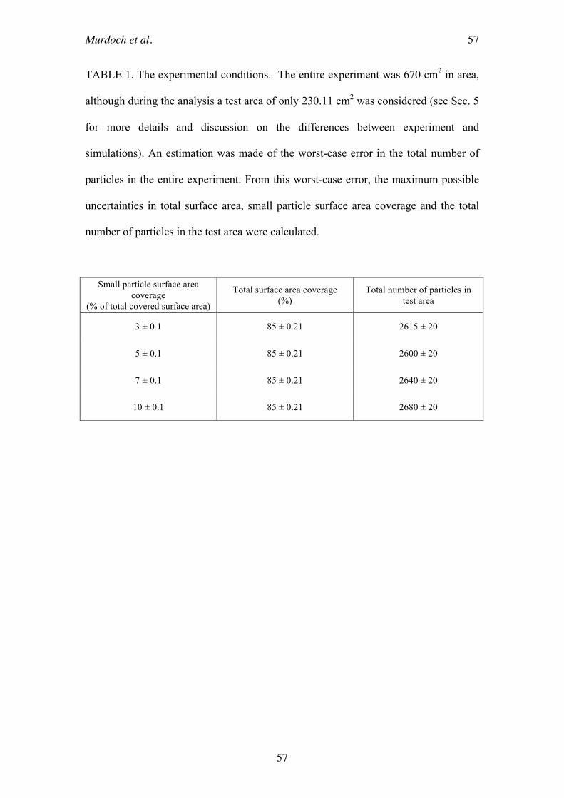
Murdoch et al.

57

57

TABLE 1. The experimental conditions. The entire experiment was 670 cm2 in area,

although during the analysis a test area of only 230.11 cm2 was considered (see Sec. 5

for more details and discussion on the differences between experiment and

simulations). An estimation was made of the worst-case error in the total number of

particles in the entire experiment. From this worst-case error, the maximum possible

uncertainties in total surface area, small particle surface area coverage and the total

number of particles in the test area were calculated.

Small particle surface area

coverage

(% of total covered surface area)

Total surface area coverage

(%)

Total number of particles in

test area

3 ± 0.1 85 ± 0.21 2615 ± 20

5 ± 0.1 85 ± 0.21 2600 ± 20

7 ± 0.1 85 ± 0.21 2640 ± 20

10 ± 0.1 85 ± 0.21 2680 ± 20

Murdoch et al.

58

58

TABLE 2. The conditions of the numerical simulations. The normal coefficient of

restitution of the particles is 0.5 (where 1.0 would mean completely elastic collisions)

and the tangential coefficient of restitution is 0.9 (where 1.0 would be completely

smooth).

Small particle surface area coverage

(% of total covered surface area)

Total surface area coverage

(%) Total number of particles

2.91 83.76 1247

4.84 83.85 1277

6.89 83.83 1307

10.16 83.63 1352

Murdoch et al.

59

59

TABLE 3. Detailed list of all differences between experiments and simulations.

PARAMETER EXPERIMENT SIMULATION

Total surface area 670.1 cm2 100.0 cm

2

Surface area considered in

analysis 214.6 cm

2 100.0 cm

2

Shape of container Circular (292 mm diameter) Square (100 mm x 100 mm)

Shape of area considered in

analysis

Rectangular (169 mm x 127

mm) Square (100 mm x 100 mm)

Shaking axis

In the z-direction with a small

acceleration (< 0.5%) in the

horizontal (x-y) plane

In the z-direction

Particle sizes Diameter tolerance of 0.025 mm Exactly 2.0 mm or 3.0 mm

diameter

Particle density 7900 kg m-3

7000 kg m-3

Particle shapes Uncertainty of 10-6

m Exactly spherical

Small particle concentration Calculated by weight for the

entire container Calculated exactly

Movement of walls during

shaking

Entire container shaken so all

container walls shaken in phase

Top and bottom walls shake in

phase, side walls are stationary

Bottom wall shape Slightly convex Exactly planar

Murdoch et al.

60

60

TABLE 4. The mean horizontal speed of one particle in a numerical simulation during

a period of 5 seconds calculated using four different methods.

Murdoch et al.

61

61

TABLE 5. The different simulations performed over the course of this study. The

parameters in bold are the baseline parameters used in this study.

Figure Captions

Figure 1. Schematic of the experiment used in Berardi et al. (2010). The container

depth is 3 mm and the separation between the top of the largest particles and the

confining lid is 0.1 mm. The base plate, container and the confining lid vibrate

together at a frequency of 125 Hz and with a maximum acceleration of 4.5 g. Note:

Figure not to scale.

Figure 2. Ray-traced images of a simulation during the vibration phase as seen from

(a) the side and (b) above. Particles are contained in a box of 100 mm # 100 mm.

There is a confining lid in the z-direction 0.1 mm above the largest particles (see Fig

1). All walls are made transparent to facilitate observation. There are two sizes of

particles: 1.5 mm radius (red) and 1 mm radius (yellow). The total surface area

coverage is 83.63%. The 1 mm radius particles cover 8.50% of the entire container

surface area (i.e., 8.50% of 100 mm2), which is equivalent to 10.16% of the total

covered surface area (i.e., 10.16% of 83.63 mm2).

Figure 3. The degree of local order (i.e., packing density) at the position of each

particle when the small particle concentration is 3%. Results are shown for both the

laboratory experiment (a) and a numerical simulation (b). Grain Boundary (GB)

regions determined using the algorithm of Berardi et al. (2010). Black signifies near-

hexagonal particle packing with !6 close to 1. Grey and white correspond to more

disordered packing with !6 < 0.7 (i.e., GB regions). See Equation (1) for the

definition of !6. Particles are not drawn to scale.

Murdoch et al.

63

63

Figure 4. The locations of all particles at the start of the vibration phase of the

numerical simulations when the small particle concentration is (a) 3% and (b) 10%.

Large (3mm) particles are white, small (2mm) particles are black. Figures are drawn

to scale. In both figures regions of crystallisation can be seen.

Figure 5. The degree of local order (i.e., packing density) at the position of each

particle in a numerical simulation when the small particle concentration is 10%. Grain

Boundary (GB) regions determined using the algorithm of Berardi et al. (2010). Black

signifies near-hexagonal particle packing with !6 close to 1. Grey and white

correspond to more disordered packing with !6 < 0.7 (i.e., GB regions). See Equation

(1) for the definition of !6. The locations of the small (2 mm) particles are all

marked with an X. The laboratory experiment results are not shown here, but in both

the experiments and the numerical simulations the small particles are almost all

located in grain boundaries. Particles are not drawn to scale.

Figure 6. Grain boundary coverage, measured as the percentage of covered surface in

grain boundaries, as a function of small particle concentration for the laboratory

experiment (open circles) and the baseline numerical simulation (filled circles). The

grain boundary coverage is calculated many times (approximately once per second)

over the duration of each simulation and experiment and the mean value is plotted

along with the standard deviation of the mean. Increasing grain boundary area with

increasing small particle concentration can clearly be seen for both data sets. The

quantitative differences are discussed in Sec. 5.

Murdoch et al.

64

64

Figure 7. The speed of one particle in a numerical simulation over a period of 0.25

seconds, calculated using three different methods: (white diamonds): the

instantaneous particle speed calculated during the numerical simulations; (black dots):

using the coordinates of the particle sampled at 125fps; (open white circles): using the

coordinates of the particle sampled at 125 fps and smoothed over 0.1 seconds.

Figure 8. The mean-square displacement (MSD) curves are shown for the laboratory

experiment with 10% small particle concentration (dotted line) and three different

numerical simulations also with 10% small particle concentration. The similar shapes

of the experimental and simulation MSD curves, and the magnitude discrepancy, are

discussed in Section 5. Also shown for comparison, and to demonstrate the

sensitivity of our simulations to different parameters (see Sec 5.5), are two extreme

10% small particle concentration numerical simulation MSD profiles; case A in which

the particles break out of their cage very early (dashed line) and case B where the

particles remained jammed over much longer timescales (dashed - dotted line). The

parameters for cases A and B are, respectively: normal coefficient of restitution of the

particles = 0.1 and 0.9; tangential coefficient of restitution of the particles = 0.5 and

0.9; normal coefficient of restitution of the walls = 0.5 and 0.9; tangential coefficient

of restitution of the walls = 0.5 and 0.9.

Figure 9. Average number of granular strings at a given time-step as a function of

additive concentration for the baseline simulation, defined as the percentage of total

area covered by the small-particle additive. The errors bars are the standard error of

the mean for one experiment at one small particle concentration. As each experiment

Murdoch et al.

65

65

is thousands of frames, we expect to sample all configurations and so report the

standard error and not the standard deviation.

Figure 10. Average granular string length in particles as a function of small particle

surface area coverage, defined as the percentage of total surface area covered by the

small-particle additive from the laboratory experiment (open circles) and the

numerical simulations (filled circles). The error bars, which are smaller than the size

of the markers, are the standard error of the mean for one experiment at one small

particle concentration.. As each experiment measures thousands of strings, we expect

to sample all configurations and so report the standard error and not the standard

deviation.

Figure 11. (a) Average number of granular strings and (b) average granular string

length at a given time-step as a function of varying external gravity for simulations

with 10% small particle concentration. The errors bars, which are sometimes smaller

than the markers, are the standard error of the mean for one experiment at one small

particle concentration. As each experiment is thousands of frames, we expect to

sample all configurations and so report the standard error and not the standard

deviation.

Figure 12. (a) Average number of granular strings and (b) average granular string

length at a given time-step as a function of varying particle density for simulations

with 10% small particle concentration and inter-particle gravity but no external

gravity. The errors bars, which are sometimes smaller than the markers, are the

standard error of the mean for one experiment at one small particle concentration. As

Murdoch et al.

66

66

each experiment is thousands of frames, we expect to sample all configurations and so

report the standard error and not the standard deviation.

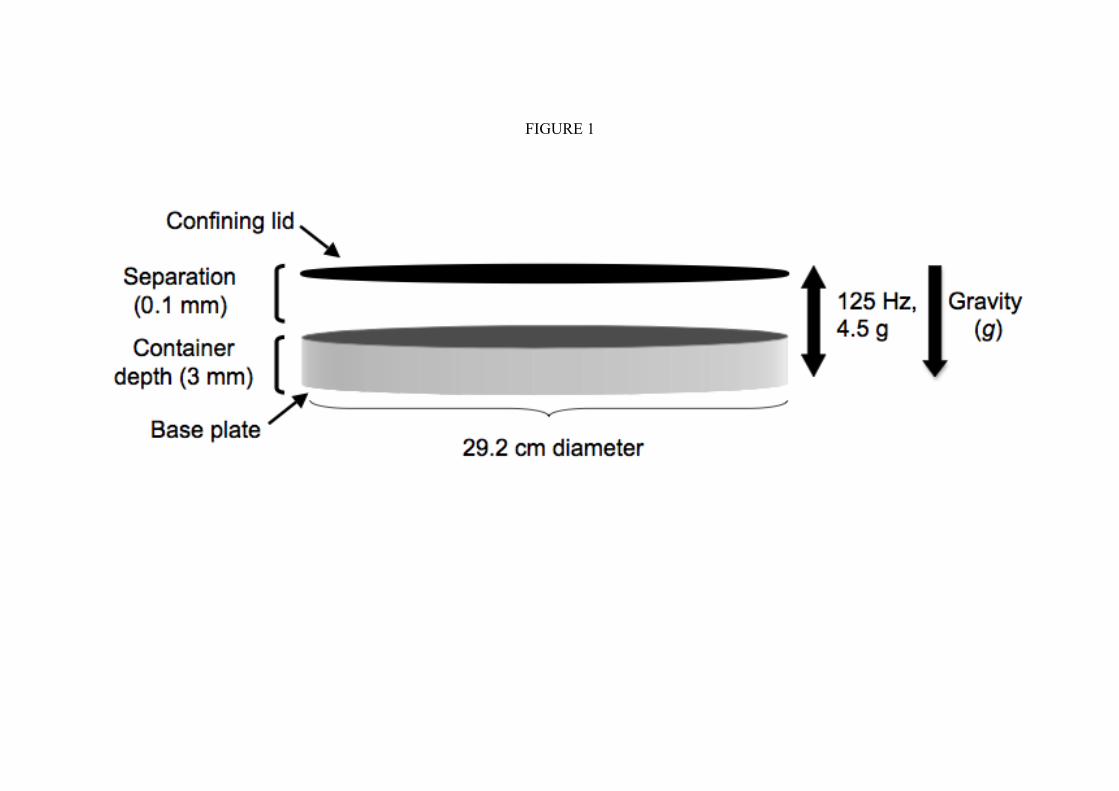
FIGURE 1

FIGURE 2

(a)

(b)

FIGURE 3

(a) (b)

Murdoch et al.

70

70

FIGURE 4

(a) (b)

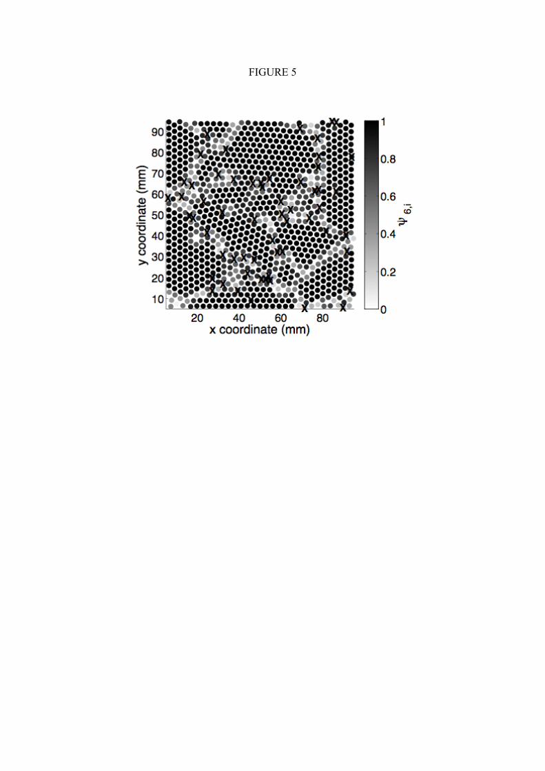
FIGURE 5

FIGURE 6

Murdoch et al.

73

73

FIGURE 7

Murdoch et al.

74

74

FIGURE 8

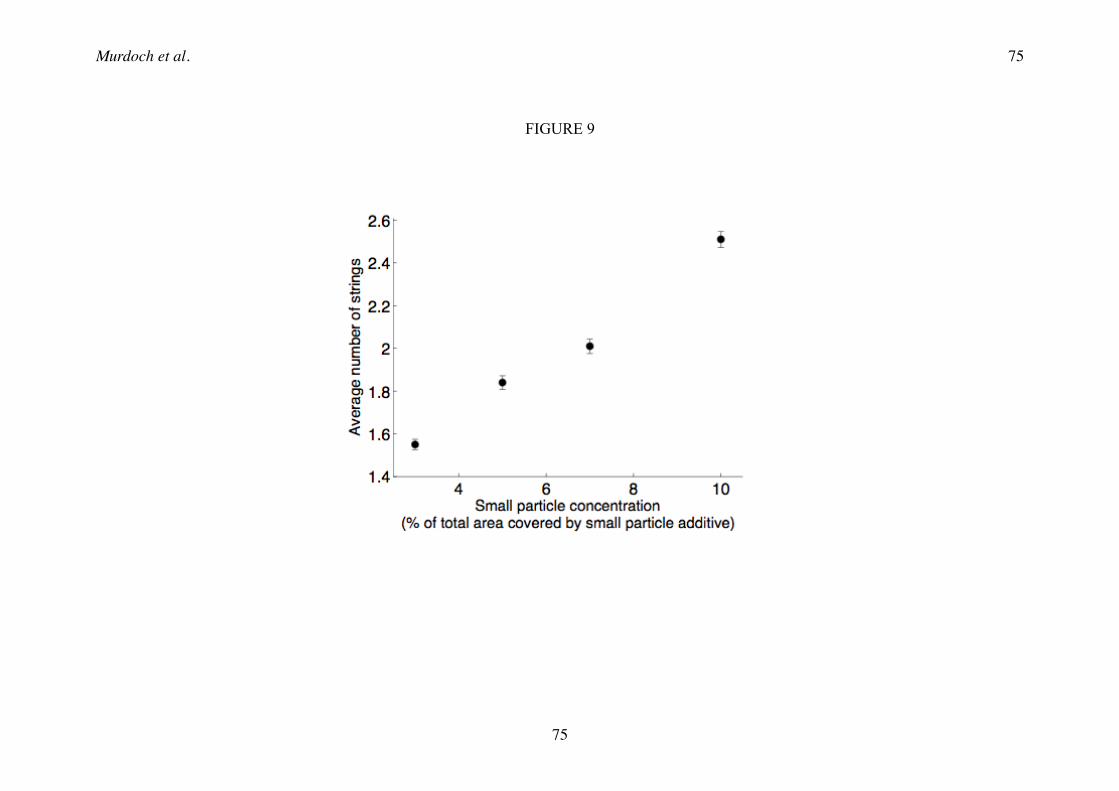
Murdoch et al.

75

75

FIGURE 9

Murdoch et al.

76

76

FIGURE 10

Murdoch et al.

77

77

FIGURE 11

(a) (b)

Murdoch et al.

78

78

FIGURE 12

(a) (b)