Numerical simulation of transient detonation structures in ...
NUMERICAL SIMULATION OF UNSTEADY NORMAL DETONATION COMBUSTION
by
AJJAY OMPRAKAS
Presented to the Faculty of the Graduate School of
The University of Texas at Arlington in Partial Fulfillment
of the Requirements
for the Degree of
MASTER OF SCIENCE IN AEROSPACE ENGINEERING
THE UNIVERSITY OF TEXAS AT ARLINGTON
MAY 2018
ii
Copyright copy by Ajjay Omprakas 2018
All Rights Reserved
iii
Acknowledgments
This thesis would not have been possible without the guidance and help of all my
supervisor professors lab mates family and friends I would like to thank my masters
supervisor Dr Donald R Wilson and PhD mentor Rahul Kumar who guided me throughout
the project without whom this thesis would not have been possible I would like to thank
Dr Endel v larve and Dr Miguel A Amaya for agreeing to be on the defense committee and
reviewing my thesis
Finally I would like to thank my family and friends for their continued support and
encouragement throughout my education and stay in UTA
May 09 2018
iv
ABSTRACT
NUMERICAL SIMULATION OF UNSTEADY NORMAL DETONATION COMBUSTION
AJJAY OMPRAKAS MS
The University of Texas at Arlington 2018
Supervising Professor Donald R Wilson
The objective of this research is to simulate normal detonation combustion which is a mode
of operation for a Pulsed Detonation Engine (PDE) A supersonic flow with stoichiometric
hydrogen-air mixture is made to impinge on a wedge thus resulting in increasing the
temperature and pressure across a shock wave leading to the formation of detonation
wave Different modes of the operations can be simulated by varying the incoming Mach
number pressure temperature and equivalence ratio For the case of normal detonation
wave mode which is an unsteady process after the detonation being initiated due to the
shock induced by the wedge the detonation wave propagates upstream in the flow as the
combustion chamber Mach number is lower than the C-J Mach number The concept of
detonation wave moving upstream and downstream is controlled by changing the incoming
flow field properties By this method the unsteady normal detonation wave is made to
oscillate in the combustion chamber leading to a continuous detonation combustion The
intention of this research is to simulate two cycles of detonation combustion in order to
determine the frequency and to obtain the variation of flow properties at the exit plain with
respect to time
v
TABLE OF CONTENTS
Acknowledgements iii
ABSTRACT iv
List of Illustrations vi
List of Tables vi
Chapter 1 INTRODUCTION 1
11 Concept of Multi-Mode Pulsed Detonation Engine 1
12 Detonation Physics and Chapman - Jouguet condition 3
13 Thermodynamics 9
Chapter 2 GOVERNING EQUATIONS 16
21 Reactive Euler equation 16
22 Thermodynamic Relation 19
23 Chemical Kinetics 23
Chapter 3 NUMERICAL METHOD 28
31 Density - based solver 28
32 Discretization and solution 30
33 Spatial Discretization 31
34 Boundary Conditions 36
35 Computational Resources 37
Chapter 4 CHEMISTRY MODELING 39
Chapter 5 GEOMETRY AND GRID STUDY 43
Chapter 6 RESULTS AND DISCUSSION 55
Chapter 7 CONCLUSION 72
Appendix A Fluent chemkin Input 74
References 77
vi
List of Illustrations
Fig 11 Multimode pulse detonation engine 2
Fig 12 Schematics of detonation 4
Fig 13 T-S diagram for different combustion model 5
Fig 14 Chapman ndash Jouguet Detonation model 6
Fig 15 Variation of Pressure and temperature in ZND Detonation 7
Fig 16 Pulsed detonation engine cycle 8
Fig 17 Flow properties across a detonation 9
Fig 18 (a) Rankine ndash Hugoniot curve 12
Fig 18 (b) Rankine ndash Hugoniot curve to calculate von Neumann pressure spike 12
Fig 31 Solving method in a density ndash based solver 29
Fig 32 F ndash cycle multigrid solver 35
Fig 33 Accessing Fluent in TACC 38
Fig 41 Time variation of mole fraction for 23 step and 11 species Hydrogen -air
reaction p = 1 atm and T = 1000 K 41
Fig 42 Density variation with respect to time 42
Fig 43 Temperature variation with respect to time 42
Fig 51 Two ndash Dimensional combustion chamber 44
Fig 52 Sod Shock tube problem (SOD) geometry 45
Fig 53 Density along x-axis at time T = 52 x 10-4 sec 45
Fig 54 Velocity along x-axis at time T = 52 x 10-4 sec 46
Fig 55 Pressure along x-axis at time T = 52 x 10-4 sec 46
Fig 56 Initial pressure and temperature contour for grid study 48
Fig 57 Pressure along x-axis at time 45 x 10-4 sec 49
vii
Fig 58 Temperature along x-axis at time 45 x 10-4 sec 49
Fig 59 Velocity along x-axis at time 45 x 10-4 sec 50
Fig 510 Detonation propagation in the grid size 003 x 10-5 m 51
Fig 511 Temperature contour in grid size 003 x 10-5 m 52
Fig 512 Velocity contour in grid size 003 x 10-5 m 52
Fig 513 Numerical schlieren imaging 53
Fig 514 Mass fraction of H2 O2 H2O 53
Fig 61 Time from 0 to 15 x 10-4 sec 59
Fig 62 (ab) Time from 15 x 10-4 to 60 x 10-4sec 60
Fig 63 Time from 60 x 10-4 to 70 x 10-4 sec 61
Fig 64 Time from 70 x 10-4 to 14 x 10-4 sec 62
Fig 65 Time from 14 x 10-4 to 24 x 10-4 sec 63
Fig 66 Propagation of the flow in case III 68
Fig 67 Variation of flow properties with respect to time for case I 69
Fig 67 Variation of flow properties with respect to time for case II 70
Fig 68 Variation of flow properties with respect to time for case III 71
viii
List of Tables
Table 11 Regions in Hugoniot curve 13
Table 21 Reaction mechaniism of hydrogen - air 26
Table 61 Case I 57
Table 62 Case II 65
Table 63 Case III 67
1
Chapter 1
INTRODUCTION
11 Concept of Multi-Mode Pulsed Detonation Engine
The Pulse Detonation Engine (PDE) has created considerable attention due to its
higher thrust potential wider operating range high thermodynamic efficiency and
its mechanical simplicity with the lack of movable parts compared to the
conventional engine[1][2] The advantages of the PDE comes from its utilization
of the detonation combustion rather than regular deflagration that has been used by
the Brayton cycle engines The detonation process is much more energetic than
deflagration combustion consisting of a shock wave propagating at supersonic
speed coupled with an induction and reaction zone whereas in a deflagration the
combustion occurs at subsonic speed[1][2][3]
But the conventional PDE cannot be operated at hypersonic speed since the inlet
compression increases the static temperature to a value greater than the
autoignition temperature of the fuel To overcome this difficulty the concept of the
multi-mode pulsed detonation engine was conceptualized by considering the best
features of various engine concepts such that it can overcome the limitations of the
individual engine concepts and provide the ability to operate over a wide range of
operating conditions from subsonic to supersonic speed This concept is illustrated
2
in the Fig 11 and it consists of four modes of operations The operating modes are
as follows - (a) an ejector-augmented pulsed detonation rocket (PDR) mode for
take-off and accelerate to moderate supersonic velocity (b) a normal detonation
wave engine (NDWE) mode for operation at flight Mach numbers from
approximately 3 to 6 where the combustion chamber Mach number is less than the
a Chapman-Jouguet Mach number for the given fuel stoichiometry condition (c)
an oblique detonation wave engine (ODWE) mode for hypersonic flight where the
combustion chamber Mach number is greater than that of the Chapman-Jouguet
Mach number for a given fuel stoichiometry condition and (d) a pulsed detonation
rocket mode for very high Mach number and altitude due to the scarcity of oxygen
for combustion[4][1][5][6]
Fig 11 Multimode pulse detonation engine
3
12 Detonation Physics and Chapman ndash Jouguet condition
A detonation wave is a complex oscillating three-dimensional cellular structure
consisting of a shock followed by an induction zone with a coupled reaction region
where the products are accompanied by a rapid release of energy As the detonation
wave propagation is supersonic in nature the reactants upstream are not affected
until the flow comes in contact with the detonation wave front As the shock passes
through the reactants it compresses heats and ignites the mixture resulting in
combustion zone propagating with the velocity of the shock The shock wave is
coupled with the reaction zone triple point transverse wave and shear layer as
shown in the Fig 12 (ab) [4][6][1][2][3] Consider a detonation wave propagating
in a tube filled with a combustible mixture that is closed at one end and opened at
the other The detonation is initiated at the closed end by a high enthalpy source
and the shock wave moves at the velocity of the detonation wave Vdet relative to
the gas chamber The thermodynamics of the process is given by T-S diagram as
shown in Fig 13
4
Fig 12 (ab) schematics of detonation
Fig 13 shows the difference between the constant pressure combustion (Brayton
cycle) constant volume combustion (Humphrey cycle) and detonation cycle The
stage 0 -1 known as the pre-compression is mandatory for a Brayton cycle but for
detonation the leading shock provides the necessary pressure rise to sustain the
combustion
5
Fig 1 3 T-S diagram for different combustion model
This complex concept of detonation is explained by two relatively simple
theoretical model The Chapman-Jouguet (CJ) and Zeldovich-von Neumann-
Doumlring (ZND) models The first theory of detonation was proposed by Chapman in
1899 and followed by Jouguet in 1905 In this theory it is assumed that the chemical
reaction takes place instantaneously inside the shock and the reaction zone length
shrink to zero as shown in Fig 14 The products are assumed to flow at a local sonic
velocity relative to the shock which is called as the Chapman ndash Jouguet condition
6
In this case the velocity of the products can be obtained by the one-dimensional
conservation equation of mass momentum and energy coupled with the chemical
reaction
Fig 14 Chapman ndash Jouguet Detonation model
An improved and more modern theory that takes into the account the effect of the
finite rate chemical reactions was originated from the work of Zeldovich von
Neumann and Doering in 1940rsquos which was later named as the ZND theory This
model of detonation is assumed to have a strong shock wave that is been coupled
to a reaction zone where a fuel and oxidizer mixture is compressed by the leading
shock and is rapidly burned which releases energy that is utilized to sustain the
propagating shock The leading shock travels at the detonation velocity and the
strength of the shock depends on the detonation velocity In this the reaction zone
is divided into two regions namely an induction zone and the heat addition zone
In the induction zone the reaction is delayed due to the finite time required to initiate
the chemical reaction The energy is released in the heat addition zone after the
7
reaction begins From Fig 15 A pressure spike is observed in the induction zone
and it is referred as the Von Neumann pressure spike [2][4][3]
Fig 15 Variation of Pressure and temperature in ZND Detonation
The concept of highly energetic detonation phenomena can be applied to the
propulsion system One such concept of engine is the pulsed detonation engine
(PDE) that was first introduced during the late 1940rsquos The ideal advantage of PDE
over the engine that follows a Brayton cycle is the high thermodynamic efficiency
thatrsquos possible to achieve by controlled combustion through detonation cycle Fig
16 represents the concept of a PDE with a nozzle at the end to expand the
combusted gas A generic PDE cycle consist of four different steps (a) filling of
8
fuel-oxidizer mixture (b) initiating the detonation (c) detonation propagation and
(d) purging of the burned gas in a blowdown process
Fig 16 Pulsed detonation engine cycle
The PDE cycle begins with the detonation chamber being filled with the fuel-
oxidizer mixture through the valve opening In the Fig 16 p0 and p1 are the ambient
and mixture pressure respectively As the detonation velocity is higher than the
velocity of fuel-oxidizer velocity during the filling process the detonation is
initiated before the mixture reaches the end of the chamber using an ignitor An
unsteady expansion wave is generated behind the detonation wave as it propagates
through the combustion medium which explains the pressure of the burned gas
being less than the Von Neumann pressure[6][7][16] An ideal detonation wave
9
will propagate at the Chapman Jouguet (CJ) velocity for the given mixture initial
condition As soon as the detonation exits the chamber a blowdown process is
started due to the pressure difference across the exit plane of the chamber which is
then followed by a purging process thatrsquos basically injecting relatively cool air into
the chamber to clear out the burned gas and to cool the chamber in order to prevent
auto-ignition of the fresh fuel-oxidizer mixture that gets injected in the following
cycle
13 Thermodynamics
In order to understand the detonation process a detailed analysis of
thermodynamics is needed For the analysis a steady state control volume of a
detonation is considered that is shown in the Fig 17 By applying the continuity
momentum and energy equation with a fluid behaving as an ideal gas to the control
volume represented in the Fig 17 gives the following [17][4][14]
Fig 17 Flow properties across a detonation
10
1205881 lowast 1199061 = 1205882 lowast 1199062 (11)
1199011 + 120588111990612 = 1199012 + 12058821199062
2 (12)
11988811990111198791 +1
21199061
2 + 119902 = 11988811990121198792 +1
21199062
2 (13)
1199011 = 120588111987711198791 (14)
1199012 = 120588211987721198792 (15)
In these equations the heat addition because of the chemical reaction is accounted
by the term q The total enthalpy of the mixture is defined as h = cpT +ho In the
above equation the heat addition is accounted by the term q = h2 ndash h1
The equation that relates the thermodynamics properties across the discontinuity is
obtained by simplifying the Rankine ndash Hugoniot equation [2][3][17]
ℎ2 minus ℎ1
= 1
2 (
1
1205882minus
1
1205881) (1199012 minus 1199011)
(16)
11
which is simplified to
1
120574 minus 1 (11990121205922 minus 11990111205921) minus
1
2 (1199012 minus 1199011)(1205922 + 1205921) minus 119902 = 0
(17)
The Rankine ndash Hugoniot curve is represented in the Eq 17 It is important to plot
the Hugoniot equation in terms of (p υ) as total enthalpy is a function of (p ρ) and
the solution lies in this plane regardless of the flow velocity The Rankine ndash
Hugoniot curve is given in the Fig 18 (a) and (b) The line that is tangential to the
Rankine ndash Hugoniot curve is the Rayleigh line representing mass flux from the Eq
18
(1199012 minus 1199011)
(11205882
minus 11205881
) = minus
(18)
12
Fig 18 (a) Rankine ndash Hugoniot curve
Fig 18 (B) Rankine ndash Hugoniot curve to calculate von Neumann pressure spike
13
The point on the Hugoniot curve where the Rayleigh line is tangential to each other
is known as the Chapman ndash Jouguet (CJ) point Theoretically there are two CJ
points on a Hugoniot curve the upper CJ point (CJu) and the lower CJ point (CJl)
They are located respectively where the Raleigh line is tangential to the Hugoniot
curve on the detonation and deflagration branch The Hugoniot curve is divided
into five regions and is represented in the Table 11
Regions in Hugoniot Characteristics Burned gas velocity
Region 1 (A - B) Strong Detonation Subsonic
Region 2 (B - C) Weak Detonation Supersonic
Region 3 (C -D) The relation is not satisfied
Region 4 (D - E) Weak deflagration Subsonic
Region 5 (E and F) Strong deflagration supersonic
Table 11 ndash Regions in Hugoniot curve
Starting from region 3 any region upstream and downstream of the given region
satisfies the Rayleigh and Hugoniot relations that is been represented in the Eq 18
and Eq 17 respectively The region 3 does not represent any real solution for the
equation In this case between the region 2 and 4 no valid Rayleigh lines could be
drawn
14
The regions 1 and 2 corresponds to strong and weak detonation regions
respectively the region 4 and 5 represents the weak and strong deflagration
respectively In case of a detonation the gas dynamic properties of the fluid are
needed to determine the burned gas propagating speed thatrsquos independent of the
actual structure of the wave This discovery was initially made by Chapman and
Jouguet in the early 20th century It was Chapman who postulated that solution
points are when the Rayleigh line is tangential to the Hugoniot curve
The region 1 represents the conditions required for a strong detonation In this case
the burned gas will be of subsonic Mach number referenced to the local
temperature The gas behind the detonation will still follow up the detonation at CJ
velocity The region 2 represents the conditions for a weak detonation with burned
gas having a supersonic Mach number The region 4 and 5 represents the condition
to have a deflagration In case of deflagration the propagating speed is determined
by the transport properties of the gasses The region 4 is a weak deflagration and
the region 5 is a strong deflagration [4][3] The conditions at the point B is the
upper C-J point and the point E represents the lower C-J point
By calculating the entropy at the C-J points for a given stoichiometry It can be
observed that a higher entropy is achieved for the conditions corresponding to the
15
upper C-J point And a lower entropy value is obtained from the conditions that
corresponds to the lower C-J point
The major importance of C-J theory is to obtain the detonation flow properties The
C-J wave propagation speed was experimentally measured by Winterberger in 2004
and found to be within a range of 2 with the theoretical CJ theory The detonation
temperature is given by [3][17]
119879119889 = 120574119889
2120574119889 + 1 (
119862119901119906
119862119901119889 119879119906 +
119902
119862119901119889)
(19)
The detonation velocity for a real gas Vd is represented as
119881119889 = radic2(120574119889 + 1)120574119889 119877119889 (119862119901119886
119862119901119889 119879119906 +
119902
119862119901119889)
(110)
When the downstream fluid is of CJ condition then the Eq (110) can be written as
119881119862119869 = 120588119862119869
120588119906 radic120574119862119869 119877119862119869 119879119862119869
(111)
16
Chapter 2
GOVERNING EQUATIONS
To simulate of a flow with a reacting gas mixture the chemical reaction between
the gases need to be modeled together with the fluid dynamics For example in the
case of detonation or combustion the basic equations of the reactive flow are the
conservation of the mass energy and momentum along with the change in
composition of gas mixture due to reaction[4][5][17]
21 Reactive Euler equation
Ignoring viscosity heat transfer diffusion radiation and body forces the governing
equation for a compressible reactive flow are the reactive Euler equation
[4][17][25] The axisymmetric reactive Euler equation are used for modeling the
PDEs combustion chamber In actuality the detonation is characterized by a three-
dimensional cellular structure which these equations lack the physical makeup to
capture Since the research is to identify the gas dynamic of various flow features
the axisymmetric model representation will work for our case The reactive Euler
equation are given by
17
120597119928
120597119905+
120597119917
120597119909+
120597119918
120597119903+ 119919 = 119934
(21)
where the state vector Q flux vector in the x-direction F flux vector in r-direction
G axisymmetric term H and the species source term W are defined as
119928 =
[
120588120588119881119909
120588119881119903
120588119864120588119884119894 ]
119917 =
[
120588119894119881119909
1205881198811199092 + 119901
120588119881119909119881119903(120588119864 + 119901)119881119909
120588119881119909119884119894 ]
119918 =
[
120588119894119881119909
120588119881119909119881119903
1205881198811199032
(120588119864 + 119901)119881119903120588119881119903119884119894 ]
119919 =1
119903
[
120588119894119881119903
120588119881119909119881119903120588119881119903
2
(120588119864 + 119901)119881119903
120588119881119903119884119894 ]
119934 =
[ 0000119877119894]
(22)
18
Here ρ V E and p are the density velocity total energy per unit mass and the
pressure of the fluid respectively Ri corresponds to the net rate of production of an
individual species due to chemical reaction and i = 1hellip Ns where Ns is the number
of species The Eq 22 inherits gas dynamics and chemical reaction coupling that
is required for modeling a self-sustained detonation
The assumptions made in the 2-D reactive Euler equations are the external forces
like gravity are negligible as the force is small in a hypersonic combustion but not
in a low-speed combustion The mass diffusion due to thermal and pressure
difference and the heat transfer due to radiation and concentration difference known
as the Dufour effect is assumed to be negligible
The 1st term represents the continuity term for the flow and gas dynamics property
The last row of the source terms in Eq (22) represents the species continuity in the
mixture that is valid for a finite reaction rate The 2nd 3rd and 4th row corresponds
to the momentum in the x-direction and r-direction and the energy equation
respectively And the pressure and temperature diffusivity terms are neglected since
they are usually exceedingly small The Eq (22) describes large class of
combustion problems that are generally quite complex
19
We introduce a preconditioned pseudo-time-derivative term in Eq (21) as
120575
120575120591 int119928 119889119881
119881
+ ∮[119917 + 119918] 119889119860 + int 119919 119889119881 = 120575
120575119905 int119934 119889119881
119881119881
(23)
where t denotes the physical time step and τ denotes the pseudo-time used in the
time-marching procedure When τ tents to infinity Eq (13) will be the same as Eq
(11) The time-dependent term in Eq (13) is discretized in an implicit fashion by
a Second-order accurate backward difference in time The dual time formulation
is written in semi-discrete form as follows
[Γ
∆120591+
1205980
∆119905 120575119934
120575119928] + ∮[119917 + 119918] 119889119860
+ int 119919 119889119881 = 1
∆119905(1205980119934
119896 minus 1205981119934119899 + 1205982119934
119899minus1) 119881
(24)
22 Thermodynamics Relation
Species and Mixture The gas mixture as a whole is an ideal gas and the
properties are functions of both temperature and pressure due to rapid change in
chemical composition In terms of individual species they are considered to be
thermally perfect gas [6][10][13]
20
119888119901 119894119904 119886 119891119906119899119888119905119894119900119899 119900119891 119879119890119898119901119890119903119886119905119906119903119890 (25)
119888119907 119894119904 119886 119891119906119899119888119905119894119900119899 119900119891 119879119890119898119901119890119903119886119905119906119903119890 (26)
The enthalpy and internal energy of species are given by
ℎ119894 = ℎ119894119891
+ int 119888119901119894 119889119905119879
1198790
(27)
119890119894 = ℎ119894119891
+ int 119888119907119894 119889119905119879
1198790
(28)
where ℎ119894119891 is the heat of formation of the ith species at a reference temperature
29815K also known as the heat of formation and is normally obtained from the
thermodynamics database
The above equations Eq (27) and Eq (28) are standard form for an arbitrary ndash
order polynomial The general form of the molar specific heat works with the
thermodynamic data in the form used in the NASA CEA In this case seven
coefficients are needed for polynomial function of temperature This is expressed
in the following form
119862119901119894
119877= 1198861119879
minus2 + 1198862119879minus1 + 1198863 + 1198864119879
1 + 11988651198792 + 1198866119879
3 + 11988671198794
(29)
21
The molar enthalpy is given as
119867119894
119877119879= minus1198861119879
minus2 + 1198862119879minus1119897119899119879 + 1198863 + 1198864
119879
2+ 1198865
1198792
3+ 1198866
1198793
4+ 1198867
1198794
5
+ 1198868
119879
(210)
The entropy of the species is calculated by
119878119894
119877= minus1198861
119879minus2
2minus 1198862119879
minus1 + 1198863119897119899119879 + 1198864119879 + 1198865
1198792
2+ 1198866
1198793
3+ 1198867
1198794
4
+ 1198869
(211)
The coefficients a1 to a9 in Eq 29 ndash 211 are obtained from the thermodynamics
database that takes into account the rotational and vibrational energy of the species
over a temperature range from 200 K to 6000 K From the above equation Eq (28)-
(211) the specific heat and enthalpy of the species per unit mass are a function of
temperature and are given by
119888119901119894 = 119877
119882119894 119862119901119894
(212)
ℎ119894 = 119877119879
119882119894 119867119894
(213)
The specific heat at constant volume and internal energy is given by
22
119888119907119894 = 119888119901119894 minus119877
119882119894
(214)
119890119894 = ℎ119894 minus 119877119879
119882119894
(215)
By taking the summation of i from 1 to Ns the above four equations will provide
the thermodynamic properties of the fluid such as the specific heat at constant
pressure enthalpy specific heat at constant volume and entropy
Ideal gas equation The equation of state for an ideal gas is given by
119875 = sum120588119877119894119879
119873119904
119894=1
(216)
where
119877119946 = 119877
119882119946
(217)
where R is the universal gas constant (8314 J mol K) and ρ is the total density of
the mixture
The speed of sound is given by
119914 = radic120574119877119879 = radic120574119875
120588
(218)
Where γ is the ratio of specific heat
23
23 Chemical Kinetics
A detailed and a stable chemical model is necessary for the source term in Eq 22
is necessary in order to create an accurate numerical model of detonation Due to
rapid chemical reaction in the case a detonation right behind the shock discontinuity
creates stiffness in source terms To overcome the stiffness in the source term due
to chemical reaction and the chemical non-equilibrium the entire source terms need
to be solved simultaneously
Chemical Reaction Mechanism Taking the stoichiometry reaction of hydrogen-
air the balanced chemical reaction equation is given as
21198672 + (1198742 + 3762 1198732) rarr 21198672119874 + 3762 1198732 (219)
To attain this reaction a series of elementary reaction which represented in a step
by step sequence by which the overall reaction takes place is named as the chemical
reaction mechanism The reaction mechanism consists of the information regarding
reaction rate third body and pressure depended reaction that represents the accurate
reaction mechanism as a whole Combining all the elementary reactions will give
24
rise to the detailed reaction with lower chemical stiffness that will be used for the
numerical simulation of detonation wave
The hydrogen-air mechanism is represented in various detailed levels from a single
step two steps to a detailed 268 step reaction mechanism [11] In this study a 11
species and 23 step hydrogen-air model thatrsquos shown in Table1 is employed as a
good representation of the hydrogen-air mechanism for the required operating
condition
The general form of the chemical reaction is written in a compact form as
sum120592119894119895prime
119873119904
119894=1
119872119894 harr sum120592119894119895
119873119904
119894=1
119872119894
(220)
where i and j are the number of species and number of reactions respectively In
this relation 120592119894119895prime and 120592119894119895
represents the stoichiometric coefficient of the reactants
and products respectively
From the elementary reactions the net rate of production of a given species is given
by
119894 = sum(120592119894119895 minus 120592119894119895
prime )
119873119903
119895=1
119896119891119895 prod[119872119894]120592119894119895
119873119904
119894=1
minus 119896119887119895 prod[119872119894]120592119894119895
prime
119873119904
119894=1
(221)
25
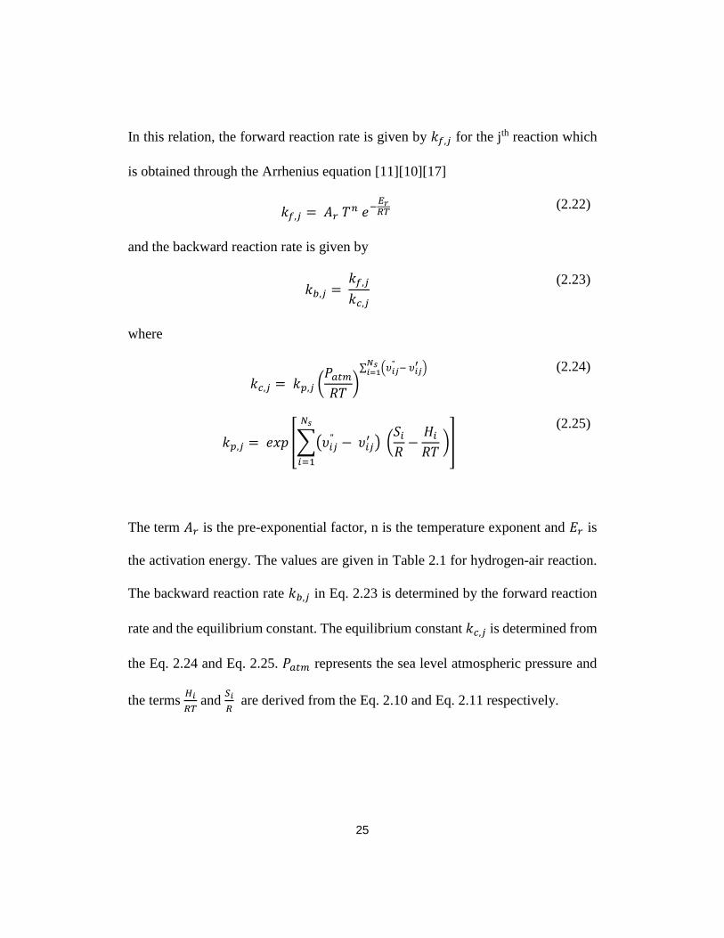
In this relation the forward reaction rate is given by 119896119891119895 for the jth reaction which
is obtained through the Arrhenius equation [11][10][17]
119896119891119895 = 119860119903 119879119899 119890minus
119864119903119877119879
(222)
and the backward reaction rate is given by
119896119887119895 = 119896119891119895
119896119888119895
(223)
where
119896119888119895 = 119896119901119895 (119875119886119905119898
119877119879)
sum (120592119894119895 minus 120592119894119895
prime )119873119904119894=1
(224)
119896119901119895 = 119890119909119901 [sum(120592119894119895 minus 120592119894119895
prime ) (119878119894
119877minus
119867119894
119877119879 )
119873119904
119894=1
]
(225)
The term 119860119903 is the pre-exponential factor n is the temperature exponent and 119864119903 is
the activation energy The values are given in Table 21 for hydrogen-air reaction
The backward reaction rate 119896119887119895 in Eq 223 is determined by the forward reaction
rate and the equilibrium constant The equilibrium constant 119896119888119895 is determined from
the Eq 224 and Eq 225 119875119886119905119898 represents the sea level atmospheric pressure and
the terms 119867119894
119877119879 and
119878119894
119877 are derived from the Eq 210 and Eq 211 respectively
26
REACTION MECHANISM A
mole-cm-sec-K b
E
calmole
H2 + O2 lt=gt OH + OH 170E+13 0 47780
OH + H2 lt=gt H2O + H 117E+09 13 3626
O + OH lt=gt O2 + H 400E+14 -05 0
O + H2 lt=gt OH + H 506E+04 267 6290
H + O2 + M lt=gt HO2 + M
H2O enhanced by 186
H2 enhanced by 286
N2 enhanced by 126
361E+17
-072
0
OH + HO2 lt=gt H2O + O2 750E+12 0 0
H + HO2 lt=gt OH + OH 140E+14 0 1073
O + HO2 lt=gt O2 + OH 140E+13 0 1073
OH + OH lt=gt O + H2O 609E+08 13 0
H + H + M lt=gt H2 + M
H2O enhanced by 00
H2 enhanced by 00
100E+18
-10
0
H + H + H2 lt=gt H2 + H2 920E+16 -06 0
H + H + H2O lt=gt H2 + H2O 600E+19 -125 0
H + OH + M lt=gt H2O + M
H2O enhanced by 50 160E+22 -2 0
H + O + M lt=gt OH + M
H2O enhanced by 50 620E+16 -06 0
O + O + M lt=gt O2 + M 189E+13 0 -1788
H + HO2 lt=gt H2 + O2 125E+13 0 0
HO2 + HO2 lt=gt H2O2 + O2 200E+12 0 0
H2O2 + M lt=gt OH + OH + M 130E+17 0 45500
H2O2 + H lt=gt HO2 + H2 160E+12 0 3800
H2O2 + OH lt=gt H2O + HO2 100E+13 0 1800
O + N2 lt=gt NO + N 140E+14 0 75800
N + O2 lt=gt NO + O 640E+09 1 6280
OH + N lt=gt NO + H 400E+13 0 0
Table 21 Reaction mechanism of Hydrogen -air
27
Third Body Reactions These reactions tend to appear in the detailed reaction
mechanism when the reactants or products is having higher bonding energy An
example for a third body reaction is
119867 + 1198742 + 119872 harr 1198671198742 + 119872 (226)
where M the third body could be 11986721198741198672 1198732 In this the energy released from the
formation of 1198671198742 from 119867 and 1198742 is carried out with the help of the third body In
the backward reaction the third body provides the required amount of energy to
break the bond in 1198671198742 to give rise to 119867 and 1198742[4][10][6] The molar concentration
with the third body efficiency is given by
119883119894 = sum120572119894119895[119872119894]
119873119904
119894=1
(227)
where the 120572119894119895 is the third body efficiency The rate of mass production Eq 221
becomes
119894 = sum(120592119894119895 minus 120592119894119895
prime )
119873119903
119895=1
[119883119894] 119896119891119895 prod[119872119894]120592119894119895
119873119904
119894=1
minus 119896119891119895 prod[119872119894]120592119894119895
prime
119873119904
119894=1
(228)
28
Chapter 3
NUMERICAL METHOD
In a chemically reacting flow there are several numerical difficulties that have to
be taken into account In a reactive flow the species continuity equations are
coupled with the governing equations that have to be solved simultaneously Due
to a wide range of time scales in the flow that leads to numerical stiffness that has
to be compensated for and there is physical complexity due to coupling of fluid and
chemical kinetics In the case of detonation due to the discontinuity and small-time
steps an extremely fine grid spacing is required to model the discontinuity across
the detonation
31 Density-based solver
In the governing equations as the flow and chemical kinetics are coupled with each
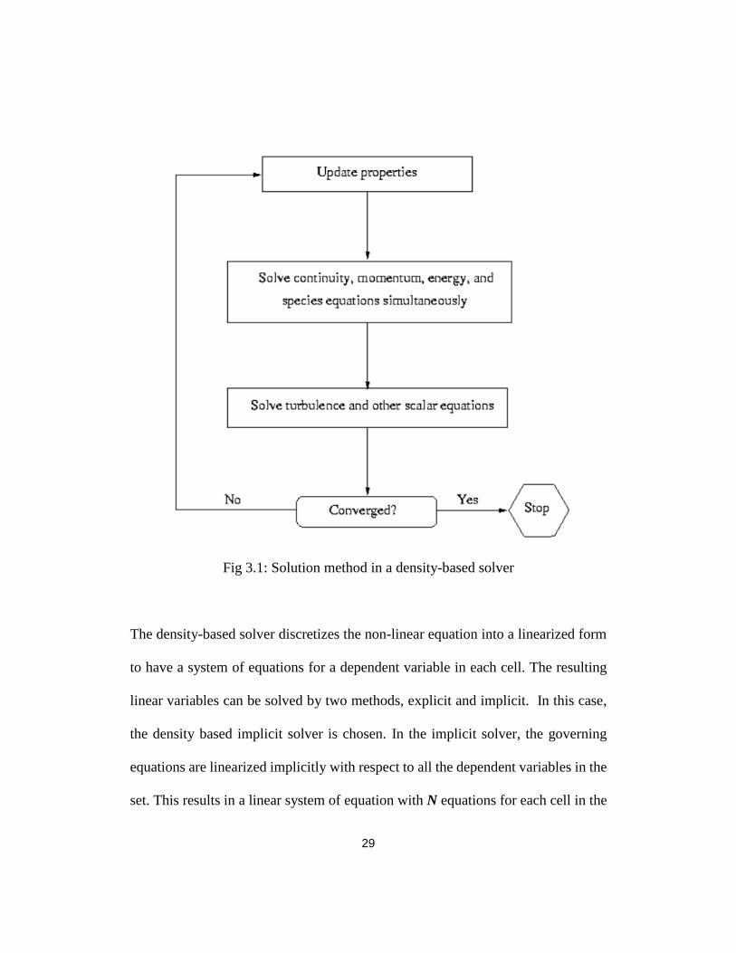
other they have to be solved simultaneously The density-based solver solves the
governing equation of continuity momentum energy and species transport
simultaneously in a coupled manner as in the flowchart described in Fig 31 Since
the governing equations are nonlinear several iterations of the solution loops have
to be performed before obtaining the converged solution [12][13]
29
Fig 31 Solution method in a density-based solver
The density-based solver discretizes the non-linear equation into a linearized form
to have a system of equations for a dependent variable in each cell The resulting
linear variables can be solved by two methods explicit and implicit In this case
the density based implicit solver is chosen In the implicit solver the governing
equations are linearized implicitly with respect to all the dependent variables in the
set This results in a linear system of equation with N equations for each cell in the
30
domain that has to be solved simultaneously where N is the number of coupled
equations in the governing set of equations For example in terms of continuity
momentum in x-direction and y-direction and energy the unknowns are p u v
and T By simultaneously solving the unknowns using a block Algebraic Multi-
Grid (AMG) solver this gives an implicit approach to solve the unknown variables
at the same time
32 Discretization and Solution
A finite volume formulation was used to convert the transport properties to an
algebraic form in the two-dimensional reactive Euler equation given in Eq 21
which is expressed as follows
int119876 119889119881
119881
+ ∮120583 120601 119889119860 = int119878 119889119881
119881
(31)
where V is the control volume A is the surface area 120583 is flux term defined as
120583 = 119865119894 + 119866119895 (32)
and 120601 is the normal unit vector defined as 120583 = 119889119909119894 + 119889119903119895
31
33 Spatial Discretization
Monotone upstream ndash centered schemes (MUSCL) In order to achieve third
order accuracy in space the MUSCL scheme [21][18] was employed The values at
face υf are been interpolated from the cell center values This is accomplished by
using upwind schemes The upwinding means the face values υf is derived from the
quantities of the cell upstream in the direction normal to the velocity Monotone
upstream-centered schemes for conservation laws (MUSCL) were used for the flow
spatial discretization The MUSCL is a created by blending the central difference
scheme and second-order upwind scheme The formulation of the MUSCL scheme
is given by
120592119891 = Θ120592119891119862119863 + (1 minus Θ)120592119891119878119874 (33)
where 120592119891119862119863 is obtained from the central difference scheme as follows
120592119891119862119863 = 1
2 (1205920 + 1205921) +
1
2 (nabla1205920 1206010119891 + nabla1205921 1206011119891)
(34)
where 0 and 1 terms represent the cell share faces The nabla terms are the reconstructed
gradient at cell 0 and 1
32
The term 120592119891119878119874 is obtained from the second order upwind stream The quantities at
the cell faces are computed using multidimensional reconstruction approach
[12][13][18] The higher order accuracy is achieved by Taylor series expansion of
the cell centered solution It is computed as follows
120592119891119878119874 = 120592 + nabla120592 ∙ 120601119891 (35)
where υ and nabla120592 are the cell center values and the gradient of the cell center values
respectively in the upstream 120601 represents the displacement vector from the
upstream of the cell face centroid The gradient term is spatially discretized by
using second order upwind scheme is the Green-Gauss cell-based which is
discussed below
Green-Gauss Theorem The gradients used for computing values of a scalar term
120601 at the cell faces center[21][18][20] The Green ndash Gauss theorem is described as
(nabla120592)119888 = 1
119907 sum120601119891 119860119891
119891
(36)
where 120601 is referred as the gradient of the scalar properties at cell center c and 120601119891
represents the value of 120601 at the cell face center is expressed as
120601119891 = 1206011198880 + 1206011198881
2
(37)
where 1206011198880 and 1206011198881 are the values at the neighboring cell centers
33
Advection Upstream Splitting Method (AUSM) The convective fluxes at each
cell F and G in Eq (31) are approximated by the flux vector splitting scheme
known as Advection upstream splitting method (AUSM) This was introduced by
Liou and Steffen in 1993 [21][19][18] This scheme first computes a cell interface
Mach number based on the characteristic speed from the adjacent cell The interface
Mach number is then used to determine the upwind extrapolation for the
convection part of the fluxes The pressure terms are obtained by splitting of Mach
number A generalized Mach number-based convection and pressure terms were
proposed by Lion [21[19][18] This provides the resolution for the shock
discontinuity and damps the oscillations at stationary and moving shocks The
scheme is expressed as follows
119865 = 119898119891120592 + 119875119894 (38)
where 119898119891 represents the mass flux through the interface The mass flux is calculated
from left to right of the interface by using the forth order polynomial
Temporal discretization For a transient simulation the governing equations Eq
(21) and Eq (22) must be discretized in both space and time This involves the
discretization of the terms at every time step ∆119905 The generic expression for the
scalar quantities with respect to time step is given by
34
120575120592
120575119905= 119865(120592)
(39)
The time derivative was calculated using a backward difference second-order
discretization is expressed as
119865(120592) = 3120592119894+1 minus 4120592119894 + 120592119894minus1
2Δ119905
(310)
where υ is the scalar quantity i is the value at the current time step i+1 is the value
at t + Δ119905 and i-1 is the value at t ndash Δ119905
An implicit time integral was selected because the scheme is unconditionally stable
with respect to time step size The downside of an implicit scheme is if the solver
was not optimized then the runtime will increase drastically The formulation to
evaluate F(υi+1) is given by
120592119894+1 minus 120592119894
Δ119905= 119865(120592119894+1)
(311)
where
120592119894+1 = 120592119894 + Δ119865(120592119894+1) (312)
High order term relaxation The importance of high order terms is to improve
the start-up and the general solution behavior of flow simulations when a higher
35
order spatial discretizationrsquos were used This also prevents convergence stalling in
many cases which leads to numerical instabilities The HOTR is used to reduce the
interaction of numerical instabilities in an aggressive solution The HOTR is written
as the first order scheme plus the additional terms from the higher order schemes
The Relaxation factor for the higher order scheme is described as follows
120593119894+1 = 120593119894 + 119891(120593119894+05 minus 120593119894) (313)
where 120593 is a generic formulation for any terms from single to higher order and 119891
is the under-relaxation term
Algebraic Multigrid (AMG) In this case a F ndash cycle multigrid was selected F-
cycle is essentially a combination of V and W cycles as described below in Fig 32
119953119955119942 119956119960119942119942119953 rarr 119955119942119956119957119955119946119940119957 rarr 119934 119940119962119940119949119942 rarr 119933 119940119962119940119949119942 rarr 119953119955119952119949119952119951119944119938119957119942 rarr 119953119952119956119957 119956119960119942119942119953
Fig 32 F ndash cycle multigrid solver
where the restriction and propagation are used based on the additive correction
strategy [21][18]
36
34 Boundary Conditions
Pressure Inlet In the case of a compressible inlet the pressure inlet evaluates the
isentropic flow relations using ideal gas relations The input total pressure P0 and
the static pressure Ps in the adjacent cells are related as
1198750 + 119875119900119901
119875119904 + 119875119900119901= (1 +
120574 minus 1
2 1198722)
120574120574minus1
(314)
where
119872 = 119881
radic120574119877119879119904
(315)
The density and the temperature at the inlet plane is from the ideal gas law that is
given as follows
120588 = 119875119904 + 119875119900119901
119877119879119904
(316)
1198790
119879119904= 1 +
120574 minus 1
2 1198722
(317)
where op is the operating condition The individual velocity components at the inlet
are derived using the direction vector components
37
Pressure Outlet This outlet condition extrapolates the values at the exit from the
interior of the domain The extrapolation is carried out by using the splitting
procedure based on the AUSM scheme [4][18][20][21]
Symmetry The geometry is taken to be 2-D axis-symmetric There are no flux
terms across the boundary with zero normal velocity component
35 Computational Resources
Generally a chemically reactive flow solution requires an extended amount of
computational time and resources are required in order to obtain a converged and
accurate solution due to the complexity in the problem The run-time of the
numerical simulation of a reactive flow is reduced by using multiple CPUrsquos with
optimum number of cores and nodes Extensively increasing the processor number
will also lead to increase in run-time as the commutation time among the processor
cores are higher than the communication between the nodes for an efficient
performance minimum communication among the processors has to be maintained
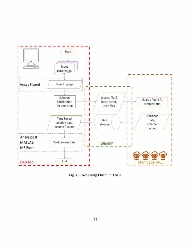
Stampede 2 from Texas Advanced Computing Center (TACC) [22][23] was
utilized remotely for running the simulations The TACC was accessed through
windows secured copy (WinSCP) protocol The flowchart in Fig 33 represents the
process involved in accessing fluent in TACC
38
Fig 33 Accessing Fluent in TACC
39
Chapter 4
CHEMISTRY MODELING
The stability of the chemical reaction plays a vital role in the detonation
combustion In order to model the chemical kinetics chemked was used which runs
Chemkin III solver in the background The results obtained from chemked is
validated by comparing with the NASA CEA results [12][13][10]
The formulas used to calculate the reaction rate is explained in section 23 The
input file for the Chemked is in the Chemkin III format [10] and was modified
according to the required case The input file for the chemical kinetics solution for
the detonation in Chemkin format is provided in the APPENDIX along with the
thermodynamic properties of the materials in the reaction which was obtained from
NASA-CEA [12] and GRI mech [13][10]
The rate change of mole fraction with respect to time is compared with THYi [20]
and Chemkin III A Fortran chemical kinetics package for analysis of gas-phase
chemical and plasma kinetics [10] with the following initial conditions of pressure
as 1 atm and temperature as 1500 K The initial mole fraction of hydrogen is 0296
oxygen is 0148 nitrogen is 0556 which corresponds to the stoichiometry for
40
hydrogen-air reaction [4][6][20] The hydrogen-air reaction mechanism considered
here is a 11 species and 23-step reaction model which has an operating range from
400 K to 6000 K This reaction takes into consideration of all the quantum modes
of energy in the molecule as the vibrational mode tends to dominate above 2800 K
for Nitrogen molecule which is near to the detonation temperature of hydrogen-air
for the given operating condition
Increasing the number of chemical steps in the model will provide a detailed
separation of the induction and reaction zone in the detonation But while
considering the global scale of the problem the complexity of the solution will
increase which in turns increases the runtime of the simulation So compromises
had to be made in selecting an appropriate reaction model for the hydrogen-air
reaction without losing the details that are required for simulating a detonation For
the above mentioned initial condition the Fig 41 provides the rate change of mole
fraction of the species with respect to time The graph was generated using MatLab
from the data that been obtained from the Chemked solver
41
Fig 41 Time variation of mole fraction for 23 step and 11 species hydrogen -air
reaction p = 1 atm and T = 1500 K
42
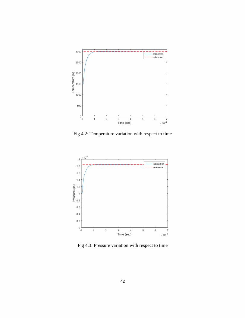
Fig 42 Temperature variation with respect to time
Fig 43 Pressure variation with respect to time
43
Chapter 5
GEOMETRY AND GRID STUDY
In this chapter we discuss about the geometry and the grid study of the 2-D
axisymmetric combustion chamber for unsteady detonation-simulation And also
the methods that are used to validate the boundary condition in order to obtain the
required results in a cold flow and the necessary steps that have been carried out
for a grid independence study for the given geometry to capture the detonation C-J
condition by checking the pre and post-shock properties along with the C-J
condition the NASA CEA [12][13]
The combustor geometry is a two-dimensional axis-symmetric combustion
chamber consisting of a wedge followed by a shock cancelation zone The wedge
angle was chosen after a flow study carried out on different wedge angles for
different modes of detonation done by Hui ndash Yuan Fan [6][4][20] The wedge angle
of 15o is selected because this lies in a complex region where the initiation of both
oblique and normal detonation wave is made possible by changing the inlet
condition of the combustion chamber The sketch of the geometry is given in Fig
51
44
Fig 51 Two ndash Dimensional combustion chamber
SOD shock tube problem This problem is being taken as a base reference in order
to check if the given initial conditions and the solver for the given geometry with
the following structured grid size are able to capture the shock along with the pre
and post-shock conditions The geometry used for the SOD problem with the grid
used is displayed in Fig 52 The initial condition of the region 4 and region 1 in the
shock tube are given as follows
(120588 120592 119901) = (10 010) 119894119891 0 lt 119909 lt 5
(0125 0 01) 119894119891 5 lt 119909 lt 10
(51)
45
Fig 52 SOD Shock tube problem (SOD) geometry
The plots in Fig (53) (54) (55) represents the ρυ p at a given time are expressed
in a was it been expected From this it can be inferred that the given geometry with
the following grid size of 009 mm with a time step of 10-5 sec is capable of
capturing the shock with the above-mentioned boundary condition
Fig 53 Density along x-axis
46
Fig 54 velocity along x-axis
Fig 55 pressure along x-axis
47
Grid independence study The grid independence study is important for modeling
a detonation as the detonation wave speed is strongly dependent on the grid spacing
[6][20]and this also helps in analyzing an appropriate grid size so the detonation is
not inadequately resolved which leads to divergence and improper results or highly
resolved which increases the total time but with just 1 or 2 variations in the
required output For the grid independence study a model which measures 10 x
1449 cm2 in length and height was created with a grid sizing of 01 009 007
003 mm The entire geometry was initialized with the stoichiometric hydrogen-air
mixture with was solved by the chemical kinetics that has been discussed in chapter
4 with the pressure of 1 atm and temperature of 700 K The CJ conditions and
detonation parameters for stoichiometric hydrogen-air mixture at the given initial
condition is obtained from NASA-CEA which are 119901
1199011 is 6631 and
119879
1198791 is 4291 119901
and 119879 are the post-detonation pressure and temperature were 119901 equates to 671900
pa and 119879 equates to 300347 K [12][13] To initiate detonation in the tube a high
enthalpy region of pressure 40 atm and temperature 4000 K was patched at the
closed end of the tube that has been shown in Fig 56 and the other end is set to be
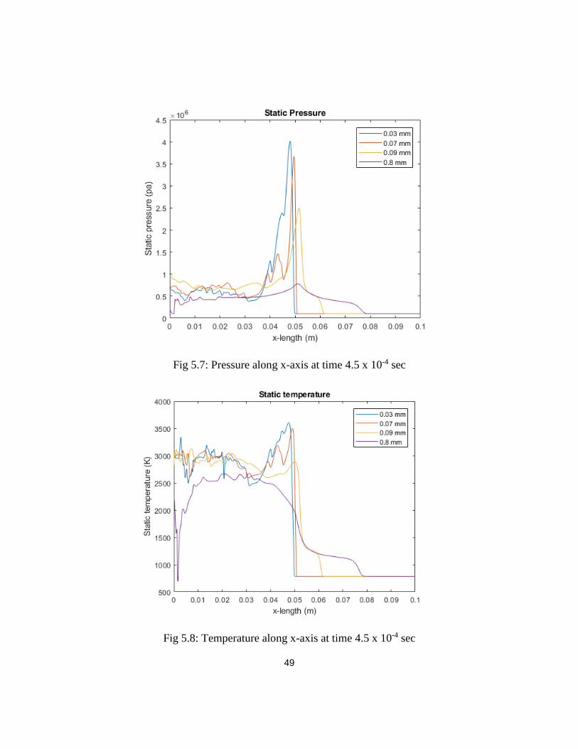
a pressure outlet to atmosphere condition The Fig 57 58 59 are the graph
comparison for pressure temperature and velocity respectively at a given time
52x10-4 seconds It can be seen that grid size plays an important role in achieving
CJ condition for the given condition and chemical reaction As it can be observed
48
from the Fig (57)(58) grid size 003 mm is the preferred grid size for capturing the
detonation
Fig 56 Initial pressure and temperature contour for grid study
49
Fig 57 Pressure along x-axis at time 45 x 10-4 sec
Fig 58 Temperature along x-axis at time 45 x 10-4 sec
50
Fig 59 velocity along x-axis at time 45 x 10-4 sec
The fluctuations of values in the Fig 57 ndash 59 are due to the interaction of shear
layer after the detonation cell that is visible in the Fig 511 ndash 513 the oscillations
in the values can be reduced by reducing the grid size or by using an Adaptive Mesh
Refinement (AMR)
51
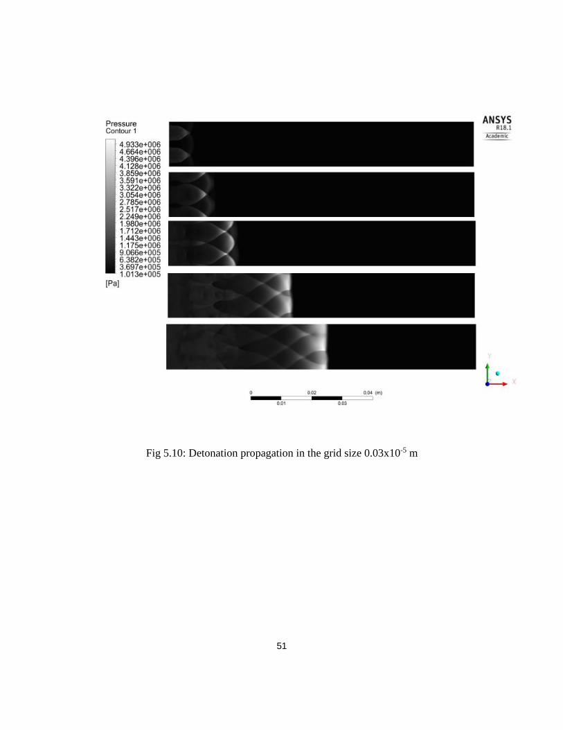
Fig 510 Detonation propagation in the grid size 003x10-5 m
52
Fig 511 Temperature contour in grid size 003 m x10-5 m
Fig 512 Velocity contour in grid size 003 x10-5 m
53
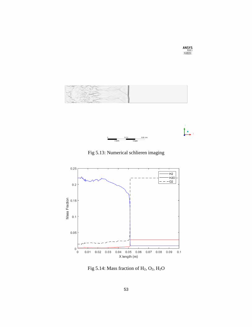
Fig 513 Numerical schlieren imaging
Fig 514 Mass fraction of H2 O2 H2O
54
The Fig (510) (511) (512) (514) are the representation of pressure temperature
velocity heat of reaction and mass fraction of species (H2 O2 H2O) respectively
for geometry with the grid size of 003 mm The Fig 51 represents the combustion
chamber which was meshed with a grid sizing of 003 x 10-5 m The total number
of cells is 2458464 and nodes is 2462005 The schematic of a two-dimensional
combustion chamber has been described in the Fig 51
55
Chapter 6
RESULTS AND DISCUSSION
The results were analyzed and post-processed using ANSYS CFD-Post
[18][20][22] and the numerical schlieren was created by using paraview In a
simulation of unsteady normal detonation the concept of detonation strength had
to be understood properly As its known that if the detonation incoming Mach
number (M35) is less than the CJ Mach number (MCJ) for the given stoichiometry
condition the detonation wave tends to move upstream in the combustion chamber
and on the other hand if the detonation incoming Mach number (M35) is higher
than the CJ Mach number (MCJ) for the given stoichiometry condition then the
detonation tends to move downstream along with the flow [4][6][15] The above
property of detonation was utilized in order to move the detonation wave upstream
and downstream inside the combustion chamber As the detonation strength
depends on the detonation chamber incoming Mach (M3) the M3 is varied by fixing
the flow inlet properties namely the pressure temperature and velocity to a
particular value in a cycle and varying the mass fraction of the fuel
For the case - I the MCJ equals to 3108 for a stoichiometric hydrogen-air with
pressure 101325 Pa and temperature 700 K as initial condition The combustion
chamber incoming Mach number 35 will have M35 equivalent to 2669 due to the
56
presence of oblique shock formed by the wedge With M35 being less that MCJ the
detonation wave would propagate upstream If the fuel is turned off that would
make the incoming flow to purge the combustion chamber and would convert the
propagating detonation wave to a propagating blast wave This blast wave will
eventually die off with no fuel in the incoming flow The problem faced in this
scenario was the length required by the blast wave to reduce in strength and die off
was longer than the length anticipated which was solved by changing the incoming
flow equivalence ratio to 05 instead of purging the chamber The MCJ equals to
282 for an equivalence ratio of 05 with the same initial conditions The change in
γ makes the combustion chamber incoming Mach number to 38 that with have a
M35 equal to 291 The M3 being larger than MCJ the detonation wave will propagate
downstream with the flow This method of NDW will oscillate the detonation wave
inside the combustion chamber and will produce a constant flow properties at the
combustion exit plain
Flow of this chapter is going to be as follows first explaining the different cases
for an unsteady normal detonation wave combustion which provides the cycle
time The cases are varied according to their initial conditions variables namely
pressure temperature and velocity The final part of the chapter is to analyze the
variation in pressure temperature and velocity ratios with respect to time at the exit
57
of the combustion chamber The Table 61 62 63 consists of the initial conditions
for the different cases
Case I
Equivalence ratio Inlet condition Time steps elapsed time
(sec)
Equivalence ratio - 1
Pressure ndash 101325 pa
Temperature ndash 800 K
Mach number ndash 35
Velocity ndash 2304874 msec
0 to 1500
15 x 10-4
Equivalence ratio ndash 05
Pressure ndash 101325 pa
Temperature ndash 800 K
Mach number ndash 38
Velocity ndash 2303281 msec
1500 to 7000
55 x 10-4
Equivalence ratio ndash 1
Pressure ndash 101325 pa
Temperature ndash 800 K
Mach number ndash 35
Velocity ndash 2304874 msec
7000 to 8000
1 x 10⁻⁴
Equivalence ratio ndash 05
Pressure ndash 101325 pa
Temperature ndash 800 K
Mach number ndash 38
Velocity ndash 2303281 msec
8000 to 11500
35 x 10-4
Equivalence ratio - 1
Pressure ndash 101325 pa
Temperature ndash 800 K
Mach number ndash 35
Velocity ndash 2304874 msec
11500 to 12500
1 x 10⁻⁴
Table 61 case I
58
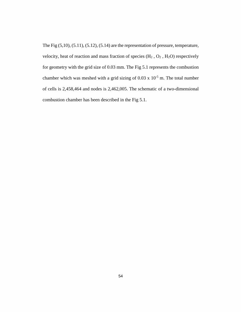
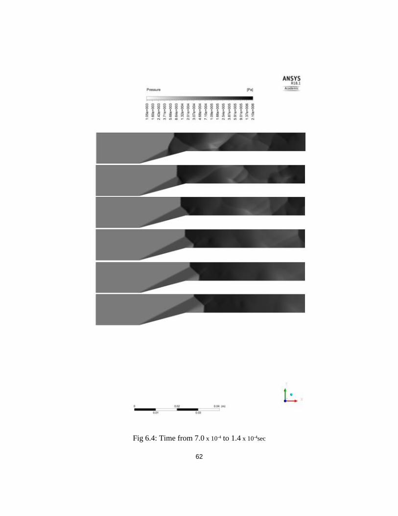
CASE I In this case as mentioned in Table 61 the initial conditions are static
pressure in the combustion chamber is 101325 Pa the static temperature is 800 K
with a Mach number of 35 that gives the velocity in x-axis at the inlet to be 2304
msec the equivalence ratio for this cycle φ is 1 It is necessary to have a similar
flow time step and chemical time step in order to avoid the instabilities This
requires the flow to have a time step of a 10-7 sec which is the appropriate time
step for a detonation with the specified chemical kinetics of hydrogen-air
[2][20][6] In this case the M3 is less than the MCJ which causes the detonation to
propagate upstream The detonation should be made to move downstream before it
crosses the wedge because if the detonation is upstream of the wedge due to the
presence of a strong normal shock in front of the reaction zone which in turn causes
the detonation to propagate upstream no matter what the inlet equivalence ratio is
set The next cycle starts when the equivalence ratio φ is changed to 05 while
maintaining the same inlet pressure temperature and velocity This causes the
Mach number to go up to 38 which makes the M3 to be higher than MCJ A single
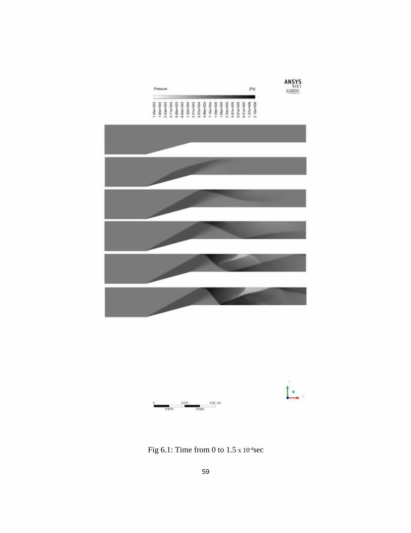
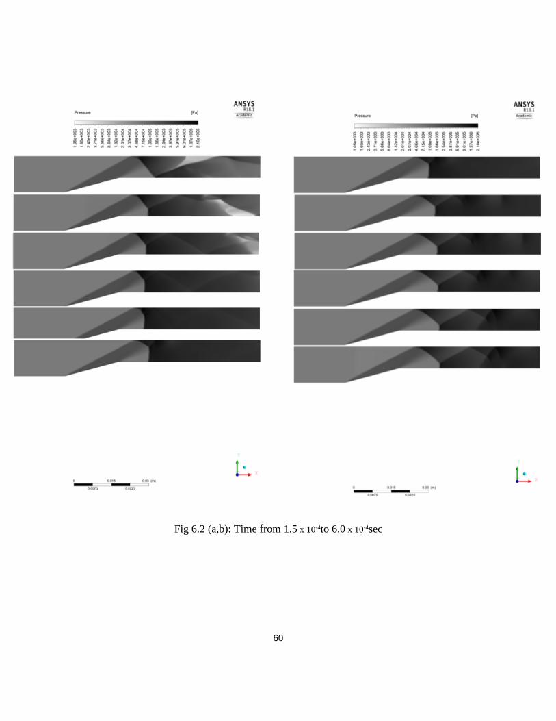
cycle time is the addition of first and second stage elapsed time The evolution of the
flow from initiation and propagation of an unsteady detonation wave with respect
to time is shown in the Fig 61 ndash 65
59
Fig 61 Time from 0 to 15 x 10-4sec
60
Fig 62 (ab) Time from 15 x 10-4to 60 x 10-4sec
61
Fig 63 Time from 60 x 10-4to 70 x 10-4 sec
62
Fig 64 Time from 70 x 10-4 to 14 x 10-4sec
63
Fig 65 Time from 14 x 10-4 to 24 x 10-4 sec
64
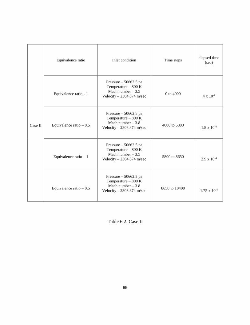
CASE II The initial conditions and the cycle time is mentioned in Table 62 The
methodology is similar to the CASE 1 but the difference is in the initial conditions
The initial conditions for this case are a static pressure in the combustion chamber
of 506625 Pa which corresponds to a high-altitude flight with a static temperature
of 800 K Mach number of 35 with an equivalence ratio of 1 This equates to a flow
velocity at the combustor inlet of 2304 msec The second cycle of this case starts
when the equivalence ratio is reduced to 05 and the pressure temperature and
velocity are maintained at the same values which increases the flow Mach number
to 379 The propagation of the flow is similar to that of the case I with minor
variation in the cycle time
65
Case II
Equivalence ratio Inlet condition Time steps elapsed time
(sec)
Equivalence ratio - 1
Pressure ndash 506625 pa
Temperature ndash 800 K
Mach number ndash 35
Velocity ndash 2304874 msec
0 to 4000
4 x 10⁻⁴
Equivalence ratio ndash 05
Pressure ndash 506625 pa
Temperature ndash 800 K
Mach number ndash 38
Velocity ndash 2303874 msec
4000 to 5800
18 x 10-4
Equivalence ratio ndash 1
Pressure ndash 506625 pa
Temperature ndash 800 K
Mach number ndash 35
Velocity ndash 2304874 msec
5800 to 8650
29 x 10-4
Equivalence ratio ndash 05
Pressure ndash 506625 pa
Temperature ndash 800 K
Mach number ndash 38
Velocity ndash 2303874 msec
8650 to 10400
175 x 10-4
Table 62 Case II
66
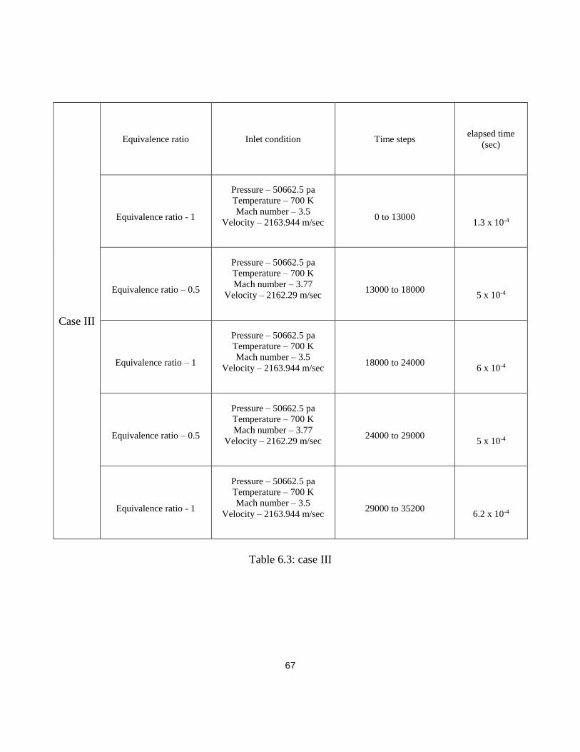
CASE III The initial conditions and the cycle time are mentioned in Table 63
The methodology is similar to the above cases the difference is in the initial
conditions The initial condition of this case is static pressure in the combustion
chamber is 506625 pa which represents a high-altitude combustion With a
temperature of 700 K flow Mach number of 35 and an equivalence ratio of 1 This
equates the flow velocity at the combustor chamber inlet to be 2163 msec The
second cycle of this case starts when the equivalence ratio is reduced to 05 and
with the pressure temperature and velocity maintained at the same value this
increases the flow Mach number to 377 The propagation of the flow is different
in this case when compared to the case I and case II because in this case the
enthalpy is lower than the previous cases This causes the detonation to be initiated
at the downstream from the wedge The propagation of the flow for two continuous
cycles are shown in Fig 66
67
Case III
Equivalence ratio Inlet condition Time steps elapsed time
(sec)
Equivalence ratio - 1
Pressure ndash 506625 pa
Temperature ndash 700 K
Mach number ndash 35
Velocity ndash 2163944 msec
0 to 13000
13 x 10-4
Equivalence ratio ndash 05
Pressure ndash 506625 pa
Temperature ndash 700 K
Mach number ndash 377
Velocity ndash 216229 msec
13000 to 18000
5 x 10⁻⁴
Equivalence ratio ndash 1
Pressure ndash 506625 pa
Temperature ndash 700 K
Mach number ndash 35
Velocity ndash 2163944 msec
18000 to 24000
6 x 10⁻⁴
Equivalence ratio ndash 05
Pressure ndash 506625 pa
Temperature ndash 700 K
Mach number ndash 377
Velocity ndash 216229 msec
24000 to 29000
5 x 10⁻⁴
Equivalence ratio - 1
Pressure ndash 506625 pa
Temperature ndash 700 K
Mach number ndash 35
Velocity ndash 2163944 msec
29000 to 35200
62 x 10-4
Table 63 case III
68
Fig 66 Propagation of the flow in case III
69
Exit condition with respect to time It is important to check the variation of flow
properties at the exit plane with respect to time in the cycle because the combustion
by normal detonation is an unsteady process By examining the exit conditions of
the combustion chamber with an extended time scale the pressure appears to
approach a steady state in case 1 Then by tweaking the inlet condition and
equivalence ratio it was made possible to achieve a steady exit plain flow property
with an unsteady normal detonation The Fig 67 represents the flow properties at
the exit of combustion chamber varying in time for case 1 Fig 68 for case 2 and
Fig 69 for case 3
Fig 67 Variation of flow properties with respect to time for case I
70
Fig 68 Variation of flow properties with respect to time for case II
71
Fig 69 Variation of flow properties with respect to time for case III
72
Chapter 7
CONCLUSION
Simulation of the motion od an unsteady normal detonation combustion wave was
evaluated computationally by using Fluent 181 The physics of detonation and the
chemical reactions were understood and engineered to simulate the cases of
unsteady detonation combustion In the different cases of normal detonation
combustion that has been mentioned in chapter 6 the initial flow properties namely
the pressure temperature and velocity are maintained constant all along the
process The direction of the propagating unsteady detonation wave depends on M3
as mentioned in chapter 6 The M3 value is changed by adjusting the mass fraction
of the incoming fuel By controlling the equivalence ratio the normal detonation
wave is made to oscillate inside the combustion chamber From the elapsed time of
each cycle it can be noted that the theoretical frequency that could be achieved by
oscillating unsteady detonation wave for combustion is higher than that of the
generic Pulsed detonation engine The theoretical frequency achieved in this
detonation combustion is 2200 Hz in Case I 2170 Hz in Case II and 909 Hz in Case
III This is much higher than the typical 100 Hz frequency that is observed in
conventional pulse detonation engine
73
From Figs 67 ndash 69 it can be inferred that the flow properties at the exit of the
combustion chamber are nearly constant even though in the presence of an unsteady
normal detonation wave
As for future work to find the operating range of the unsteady normal detonation
combustion by varying the inlet flow properties namely pressure temperature and
velocity along a typical constant q trajectory By using different fuels other than
hydrogen would provide the ratio of exit to inlet flow properties of the combustion
chamber
74
APPENDIX A
Fluent Chemkin Input
Reaction Mechanism Input file
ELEMENTS
H 100794
O 15999
N 14007
END
Species 11
SPECIES
H H2 H2O H2O2 HO2 N N2 NO O O2 OH
END
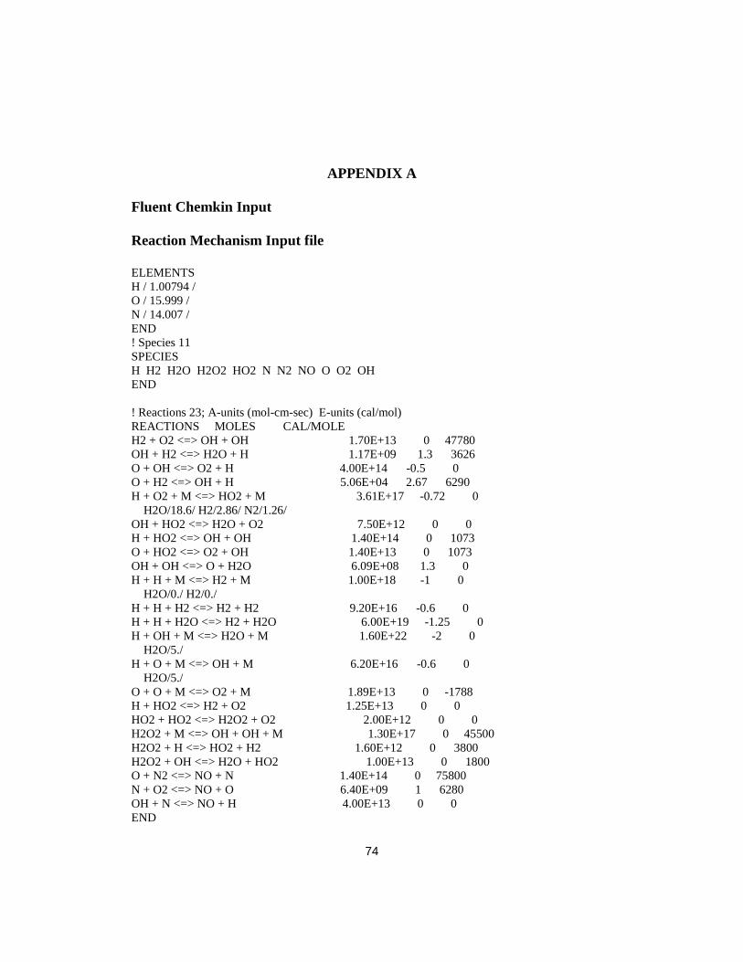
Reactions 23 A-units (mol-cm-sec) E-units (calmol)
REACTIONS MOLES CALMOLE
H2 + O2 lt=gt OH + OH 170E+13 0 47780
OH + H2 lt=gt H2O + H 117E+09 13 3626
O + OH lt=gt O2 + H 400E+14 -05 0
O + H2 lt=gt OH + H 506E+04 267 6290
H + O2 + M lt=gt HO2 + M 361E+17 -072 0
H2O186 H2286 N2126
OH + HO2 lt=gt H2O + O2 750E+12 0 0
H + HO2 lt=gt OH + OH 140E+14 0 1073
O + HO2 lt=gt O2 + OH 140E+13 0 1073
OH + OH lt=gt O + H2O 609E+08 13 0
H + H + M lt=gt H2 + M 100E+18 -1 0
H2O0 H20
H + H + H2 lt=gt H2 + H2 920E+16 -06 0
H + H + H2O lt=gt H2 + H2O 600E+19 -125 0
H + OH + M lt=gt H2O + M 160E+22 -2 0
H2O5
H + O + M lt=gt OH + M 620E+16 -06 0
H2O5
O + O + M lt=gt O2 + M 189E+13 0 -1788
H + HO2 lt=gt H2 + O2 125E+13 0 0
HO2 + HO2 lt=gt H2O2 + O2 200E+12 0 0
H2O2 + M lt=gt OH + OH + M 130E+17 0 45500
H2O2 + H lt=gt HO2 + H2 160E+12 0 3800
H2O2 + OH lt=gt H2O + HO2 100E+13 0 1800
O + N2 lt=gt NO + N 140E+14 0 75800
N + O2 lt=gt NO + O 640E+09 1 6280
OH + N lt=gt NO + H 400E+13 0 0
END
75
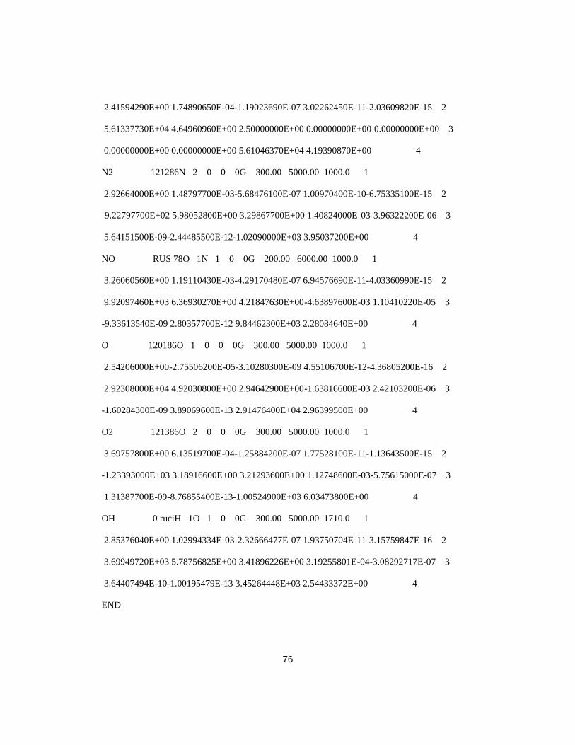
Thermodynamics data base
THERMO
300000 1000000 5000000
H 120186H 1 0 0 0G 30000 500000 10000 1
250000000E+00 000000000E+00 000000000E+00 000000000E+00 000000000E+00 2
254716300E+04-460117600E-01 250000000E+00 000000000E+00 000000000E+00 3
000000000E+00 000000000E+00 254716300E+04-460117600E-01 4
H2 121286H 2 0 0 0G 30000 500000 10000 1
299142300E+00 700064400E-04-563382900E-08-923157800E-12 158275200E-15 2
-835034000E+02-135511000E+00 329812400E+00 824944200E-04-814301500E-07 3
-947543400E-11 413487200E-13-101252100E+03-329409400E+00 4
H2O 20387 H 2O 1 0 0G 30000 500000 10000 1
267214600E+00 305629300E-03-873026000E-07 120099600E-10-639161800E-15 2
-298992100E+04 686281700E+00 338684200E+00 347498200E-03-635469600E-06 3
696858100E-09-250658800E-12-302081100E+04 259023300E+00 4
H2O2 120186H 2O 2 0 0G 30000 500000 10000 1
457316700E+00 433613600E-03-147468900E-06 234890400E-10-143165400E-14 2
-180069600E+04 501137000E-01 338875400E+00 656922600E-03-148501300E-07 3
-462580600E-09 247151500E-12-176631500E+04 678536300E+00 4
HO2 L 589H 1O 2 0 0G 20000 350000 10000 1
401721090E+00 223982013E-03-633658150E-07 114246370E-10-107908535E-14 2
111856713E+02 378510215E+00 430179801E+00-474912051E-03 211582891E-05 3
-242763894E-08 929225124E-12 294808040E+02 371666245E+00 4
N L 688N 1 0 0 0G 20000 600000 10000 1
76
241594290E+00 174890650E-04-119023690E-07 302262450E-11-203609820E-15 2
561337730E+04 464960960E+00 250000000E+00 000000000E+00 000000000E+00 3
000000000E+00 000000000E+00 561046370E+04 419390870E+00 4
N2 121286N 2 0 0 0G 30000 500000 10000 1
292664000E+00 148797700E-03-568476100E-07 100970400E-10-675335100E-15 2
-922797700E+02 598052800E+00 329867700E+00 140824000E-03-396322200E-06 3
564151500E-09-244485500E-12-102090000E+03 395037200E+00 4
NO RUS 78O 1N 1 0 0G 20000 600000 10000 1
326060560E+00 119110430E-03-429170480E-07 694576690E-11-403360990E-15 2
992097460E+03 636930270E+00 421847630E+00-463897600E-03 110410220E-05 3
-933613540E-09 280357700E-12 984462300E+03 228084640E+00 4
O 120186O 1 0 0 0G 30000 500000 10000 1
254206000E+00-275506200E-05-310280300E-09 455106700E-12-436805200E-16 2
292308000E+04 492030800E+00 294642900E+00-163816600E-03 242103200E-06 3
-160284300E-09 389069600E-13 291476400E+04 296399500E+00 4
O2 121386O 2 0 0 0G 30000 500000 10000 1
369757800E+00 613519700E-04-125884200E-07 177528100E-11-113643500E-15 2
-123393000E+03 318916600E+00 321293600E+00 112748600E-03-575615000E-07 3
131387700E-09-876855400E-13-100524900E+03 603473800E+00 4
OH 0 ruciH 1O 1 0 0G 30000 500000 17100 1
285376040E+00 102994334E-03-232666477E-07 193750704E-11-315759847E-16 2
369949720E+03 578756825E+00 341896226E+00 319255801E-04-308292717E-07 3
364407494E-10-100195479E-13 345264448E+03 254433372E+00 4
END
77
REFERENCE
[1] Munipalli R Shankar V Wilson DR Kim H Lu FK and Hagseth P ldquoA
Pulsed Detonation Based Multimode Engine Conceptrdquo AIAA Paper 2001-1786
2001
[2] Lee J H S 2008 The Detonation Phenomenon Cambridge New York
[3] Wildon Fickett and William C Davis University of California Press Berkeley
‐ Los Angeles ‐ London 1979 ldquoDetonationrdquo
[4] Fan HY and Lu FK 2008 ldquoNumerical modeling of oblique shock and
detonation waves induced in a wedged channelrdquo Journal of Aerospace
Engineering 222(5) pp 687ndash703
[5] Jin L Fan W Wang K and Gao Z ldquoReview on the recent development of
multi-mode combined detonation enginerdquo International Journal of Turbo amp Jet
Engines vol 30 no 3 pp 303ndash312 2013
[6] Heiser W and Pratt D ldquoThermodynamic Cycle Analysis of Pulse Detonation
Enginesrdquo Journal of Propulsion and Power vol 18 no 1 2002 pp 68-76
[7] Bussing T R A and Pappas G 1996 ldquoPulse Detonation Engine Theory and
Conceptsrdquo Vol 165 of Progress in Aeronautics and Astronautics AIAA Reston
Virginia pp 421 ndash 472
78
[8] Kim H W Lu KL Anderson DA and Wilson DR ldquoNumerical simulation
of detonation process in a tube Computational Fluid Dynamics Journal vol 12
no 2 pp 227 - 241 2003
[9] Rogers RC and Chinitz W ldquoUsing a global hydrogen-air combustion model
in turbulent reacting flow calculations AIAA Journal vol 21 no 4 pp 586 - 592
1983
[10] Kee RJ Rupley F M and Ellen Meeks Thermal and Plasma Processes
Department and James A Miller Combustion Chemistry Department
ldquoCHEMKIN-III A FORTRAN chemical kinetics package for the analysis of gas
phase chemical and plasma kineticsrdquo pg 134
[11] Kee RJ Miller JA and Jereson Chemkin A general purpose problem
independent transportable Fortran chemical kinetics code package Sandia
National Laboratories Tech Rep SAND 80-8003 1986
[12] Gordon S and McBride BJ ldquoComputer program for calculation of complex
chemical equilibrium compositions and application I Analysisrdquo Tech Rep NASA
RP1311 1976 [Online] Available httpwwwlercnasagovWWWCEAWeb
[13] Morley C GASEQ A chemical equilibrium program [Online] Available
httpwwwgaseqcouk
[14] Berkenbosch A C (1995) Capturing detonation waves for the reactive Euler
equations Eindhoven Technische Universiteit Eindhoven DOI 106100IR445469
79
[15]M W Chase C A Davis J R Downey D J Frurip R A McDonald and
A N Syverud ldquoJANAF Thermochemical tablesrdquo Journal of Physical Chemistry
1985
[16] J O Hirschfelder C F Curtiss and R B Bird Molecular Theory of Gases
and Liquids New York John Wiley 1954
[17] J D Anderson Hypersonic and High-Temperature Gasdynamics New York
McGraw-Hill 1998
[18] 2013 Ansys fluent text command list Online Nov
[19] Castillo J E 1991 Mathematical aspects of numerical grid generation Jan
[20] T H Yi D A Anderson D R Wilson and F K Lu Numerical study of two
- dimensional viscous chemically reacting flow AIAA 2005-4868 2005
[21] Anon 2013 Ansys fluent userrsquos guide release 150 Tech rep ANSYS Inc
[22] Texas Advanced Computing Center The University of Texas at Austin 2017
Stampede User Guide
[23] Office of Information Technology The University of Texas at Arlington
2017 HPC Users Guide
[24] Bussing T and Pappas G An Introduction to Pulse Detonation Engines
AIAA Paper 1994-0263 1994

ii
Copyright copy by Ajjay Omprakas 2018
All Rights Reserved
iii
Acknowledgments
This thesis would not have been possible without the guidance and help of all my
supervisor professors lab mates family and friends I would like to thank my masters
supervisor Dr Donald R Wilson and PhD mentor Rahul Kumar who guided me throughout
the project without whom this thesis would not have been possible I would like to thank
Dr Endel v larve and Dr Miguel A Amaya for agreeing to be on the defense committee and
reviewing my thesis
Finally I would like to thank my family and friends for their continued support and
encouragement throughout my education and stay in UTA
May 09 2018
iv
ABSTRACT
NUMERICAL SIMULATION OF UNSTEADY NORMAL DETONATION COMBUSTION
AJJAY OMPRAKAS MS
The University of Texas at Arlington 2018
Supervising Professor Donald R Wilson
The objective of this research is to simulate normal detonation combustion which is a mode
of operation for a Pulsed Detonation Engine (PDE) A supersonic flow with stoichiometric
hydrogen-air mixture is made to impinge on a wedge thus resulting in increasing the
temperature and pressure across a shock wave leading to the formation of detonation
wave Different modes of the operations can be simulated by varying the incoming Mach
number pressure temperature and equivalence ratio For the case of normal detonation
wave mode which is an unsteady process after the detonation being initiated due to the
shock induced by the wedge the detonation wave propagates upstream in the flow as the
combustion chamber Mach number is lower than the C-J Mach number The concept of
detonation wave moving upstream and downstream is controlled by changing the incoming
flow field properties By this method the unsteady normal detonation wave is made to
oscillate in the combustion chamber leading to a continuous detonation combustion The
intention of this research is to simulate two cycles of detonation combustion in order to
determine the frequency and to obtain the variation of flow properties at the exit plain with
respect to time
v
TABLE OF CONTENTS
Acknowledgements iii
ABSTRACT iv
List of Illustrations vi
List of Tables vi
Chapter 1 INTRODUCTION 1
11 Concept of Multi-Mode Pulsed Detonation Engine 1
12 Detonation Physics and Chapman - Jouguet condition 3
13 Thermodynamics 9
Chapter 2 GOVERNING EQUATIONS 16
21 Reactive Euler equation 16
22 Thermodynamic Relation 19
23 Chemical Kinetics 23
Chapter 3 NUMERICAL METHOD 28
31 Density - based solver 28
32 Discretization and solution 30
33 Spatial Discretization 31
34 Boundary Conditions 36
35 Computational Resources 37
Chapter 4 CHEMISTRY MODELING 39
Chapter 5 GEOMETRY AND GRID STUDY 43
Chapter 6 RESULTS AND DISCUSSION 55
Chapter 7 CONCLUSION 72
Appendix A Fluent chemkin Input 74
References 77
vi
List of Illustrations
Fig 11 Multimode pulse detonation engine 2
Fig 12 Schematics of detonation 4
Fig 13 T-S diagram for different combustion model 5
Fig 14 Chapman ndash Jouguet Detonation model 6
Fig 15 Variation of Pressure and temperature in ZND Detonation 7
Fig 16 Pulsed detonation engine cycle 8
Fig 17 Flow properties across a detonation 9
Fig 18 (a) Rankine ndash Hugoniot curve 12
Fig 18 (b) Rankine ndash Hugoniot curve to calculate von Neumann pressure spike 12
Fig 31 Solving method in a density ndash based solver 29
Fig 32 F ndash cycle multigrid solver 35
Fig 33 Accessing Fluent in TACC 38
Fig 41 Time variation of mole fraction for 23 step and 11 species Hydrogen -air
reaction p = 1 atm and T = 1000 K 41
Fig 42 Density variation with respect to time 42
Fig 43 Temperature variation with respect to time 42
Fig 51 Two ndash Dimensional combustion chamber 44
Fig 52 Sod Shock tube problem (SOD) geometry 45
Fig 53 Density along x-axis at time T = 52 x 10-4 sec 45
Fig 54 Velocity along x-axis at time T = 52 x 10-4 sec 46
Fig 55 Pressure along x-axis at time T = 52 x 10-4 sec 46
Fig 56 Initial pressure and temperature contour for grid study 48
Fig 57 Pressure along x-axis at time 45 x 10-4 sec 49
vii
Fig 58 Temperature along x-axis at time 45 x 10-4 sec 49
Fig 59 Velocity along x-axis at time 45 x 10-4 sec 50
Fig 510 Detonation propagation in the grid size 003 x 10-5 m 51
Fig 511 Temperature contour in grid size 003 x 10-5 m 52
Fig 512 Velocity contour in grid size 003 x 10-5 m 52
Fig 513 Numerical schlieren imaging 53
Fig 514 Mass fraction of H2 O2 H2O 53
Fig 61 Time from 0 to 15 x 10-4 sec 59
Fig 62 (ab) Time from 15 x 10-4 to 60 x 10-4sec 60
Fig 63 Time from 60 x 10-4 to 70 x 10-4 sec 61
Fig 64 Time from 70 x 10-4 to 14 x 10-4 sec 62
Fig 65 Time from 14 x 10-4 to 24 x 10-4 sec 63
Fig 66 Propagation of the flow in case III 68
Fig 67 Variation of flow properties with respect to time for case I 69
Fig 67 Variation of flow properties with respect to time for case II 70
Fig 68 Variation of flow properties with respect to time for case III 71
viii
List of Tables
Table 11 Regions in Hugoniot curve 13
Table 21 Reaction mechaniism of hydrogen - air 26
Table 61 Case I 57
Table 62 Case II 65
Table 63 Case III 67
1
Chapter 1
INTRODUCTION
11 Concept of Multi-Mode Pulsed Detonation Engine
The Pulse Detonation Engine (PDE) has created considerable attention due to its
higher thrust potential wider operating range high thermodynamic efficiency and
its mechanical simplicity with the lack of movable parts compared to the
conventional engine[1][2] The advantages of the PDE comes from its utilization
of the detonation combustion rather than regular deflagration that has been used by
the Brayton cycle engines The detonation process is much more energetic than
deflagration combustion consisting of a shock wave propagating at supersonic
speed coupled with an induction and reaction zone whereas in a deflagration the
combustion occurs at subsonic speed[1][2][3]
But the conventional PDE cannot be operated at hypersonic speed since the inlet
compression increases the static temperature to a value greater than the
autoignition temperature of the fuel To overcome this difficulty the concept of the
multi-mode pulsed detonation engine was conceptualized by considering the best
features of various engine concepts such that it can overcome the limitations of the
individual engine concepts and provide the ability to operate over a wide range of
operating conditions from subsonic to supersonic speed This concept is illustrated
2
in the Fig 11 and it consists of four modes of operations The operating modes are
as follows - (a) an ejector-augmented pulsed detonation rocket (PDR) mode for
take-off and accelerate to moderate supersonic velocity (b) a normal detonation
wave engine (NDWE) mode for operation at flight Mach numbers from
approximately 3 to 6 where the combustion chamber Mach number is less than the
a Chapman-Jouguet Mach number for the given fuel stoichiometry condition (c)
an oblique detonation wave engine (ODWE) mode for hypersonic flight where the
combustion chamber Mach number is greater than that of the Chapman-Jouguet
Mach number for a given fuel stoichiometry condition and (d) a pulsed detonation
rocket mode for very high Mach number and altitude due to the scarcity of oxygen
for combustion[4][1][5][6]
Fig 11 Multimode pulse detonation engine
3
12 Detonation Physics and Chapman ndash Jouguet condition
A detonation wave is a complex oscillating three-dimensional cellular structure
consisting of a shock followed by an induction zone with a coupled reaction region
where the products are accompanied by a rapid release of energy As the detonation
wave propagation is supersonic in nature the reactants upstream are not affected
until the flow comes in contact with the detonation wave front As the shock passes
through the reactants it compresses heats and ignites the mixture resulting in
combustion zone propagating with the velocity of the shock The shock wave is
coupled with the reaction zone triple point transverse wave and shear layer as
shown in the Fig 12 (ab) [4][6][1][2][3] Consider a detonation wave propagating
in a tube filled with a combustible mixture that is closed at one end and opened at
the other The detonation is initiated at the closed end by a high enthalpy source
and the shock wave moves at the velocity of the detonation wave Vdet relative to
the gas chamber The thermodynamics of the process is given by T-S diagram as
shown in Fig 13
4
Fig 12 (ab) schematics of detonation
Fig 13 shows the difference between the constant pressure combustion (Brayton
cycle) constant volume combustion (Humphrey cycle) and detonation cycle The
stage 0 -1 known as the pre-compression is mandatory for a Brayton cycle but for
detonation the leading shock provides the necessary pressure rise to sustain the
combustion
5
Fig 1 3 T-S diagram for different combustion model
This complex concept of detonation is explained by two relatively simple
theoretical model The Chapman-Jouguet (CJ) and Zeldovich-von Neumann-
Doumlring (ZND) models The first theory of detonation was proposed by Chapman in
1899 and followed by Jouguet in 1905 In this theory it is assumed that the chemical
reaction takes place instantaneously inside the shock and the reaction zone length
shrink to zero as shown in Fig 14 The products are assumed to flow at a local sonic
velocity relative to the shock which is called as the Chapman ndash Jouguet condition
6
In this case the velocity of the products can be obtained by the one-dimensional
conservation equation of mass momentum and energy coupled with the chemical
reaction
Fig 14 Chapman ndash Jouguet Detonation model
An improved and more modern theory that takes into the account the effect of the
finite rate chemical reactions was originated from the work of Zeldovich von
Neumann and Doering in 1940rsquos which was later named as the ZND theory This
model of detonation is assumed to have a strong shock wave that is been coupled
to a reaction zone where a fuel and oxidizer mixture is compressed by the leading
shock and is rapidly burned which releases energy that is utilized to sustain the
propagating shock The leading shock travels at the detonation velocity and the
strength of the shock depends on the detonation velocity In this the reaction zone
is divided into two regions namely an induction zone and the heat addition zone
In the induction zone the reaction is delayed due to the finite time required to initiate
the chemical reaction The energy is released in the heat addition zone after the
7
reaction begins From Fig 15 A pressure spike is observed in the induction zone
and it is referred as the Von Neumann pressure spike [2][4][3]
Fig 15 Variation of Pressure and temperature in ZND Detonation
The concept of highly energetic detonation phenomena can be applied to the
propulsion system One such concept of engine is the pulsed detonation engine
(PDE) that was first introduced during the late 1940rsquos The ideal advantage of PDE
over the engine that follows a Brayton cycle is the high thermodynamic efficiency
thatrsquos possible to achieve by controlled combustion through detonation cycle Fig
16 represents the concept of a PDE with a nozzle at the end to expand the
combusted gas A generic PDE cycle consist of four different steps (a) filling of
8
fuel-oxidizer mixture (b) initiating the detonation (c) detonation propagation and
(d) purging of the burned gas in a blowdown process
Fig 16 Pulsed detonation engine cycle
The PDE cycle begins with the detonation chamber being filled with the fuel-
oxidizer mixture through the valve opening In the Fig 16 p0 and p1 are the ambient
and mixture pressure respectively As the detonation velocity is higher than the
velocity of fuel-oxidizer velocity during the filling process the detonation is
initiated before the mixture reaches the end of the chamber using an ignitor An
unsteady expansion wave is generated behind the detonation wave as it propagates
through the combustion medium which explains the pressure of the burned gas
being less than the Von Neumann pressure[6][7][16] An ideal detonation wave
9
will propagate at the Chapman Jouguet (CJ) velocity for the given mixture initial
condition As soon as the detonation exits the chamber a blowdown process is
started due to the pressure difference across the exit plane of the chamber which is
then followed by a purging process thatrsquos basically injecting relatively cool air into
the chamber to clear out the burned gas and to cool the chamber in order to prevent
auto-ignition of the fresh fuel-oxidizer mixture that gets injected in the following
cycle
13 Thermodynamics
In order to understand the detonation process a detailed analysis of
thermodynamics is needed For the analysis a steady state control volume of a
detonation is considered that is shown in the Fig 17 By applying the continuity
momentum and energy equation with a fluid behaving as an ideal gas to the control
volume represented in the Fig 17 gives the following [17][4][14]
Fig 17 Flow properties across a detonation
10
1205881 lowast 1199061 = 1205882 lowast 1199062 (11)
1199011 + 120588111990612 = 1199012 + 12058821199062
2 (12)
11988811990111198791 +1
21199061
2 + 119902 = 11988811990121198792 +1
21199062
2 (13)
1199011 = 120588111987711198791 (14)
1199012 = 120588211987721198792 (15)
In these equations the heat addition because of the chemical reaction is accounted
by the term q The total enthalpy of the mixture is defined as h = cpT +ho In the
above equation the heat addition is accounted by the term q = h2 ndash h1
The equation that relates the thermodynamics properties across the discontinuity is
obtained by simplifying the Rankine ndash Hugoniot equation [2][3][17]
ℎ2 minus ℎ1
= 1
2 (
1
1205882minus
1
1205881) (1199012 minus 1199011)
(16)
11
which is simplified to
1
120574 minus 1 (11990121205922 minus 11990111205921) minus
1
2 (1199012 minus 1199011)(1205922 + 1205921) minus 119902 = 0
(17)
The Rankine ndash Hugoniot curve is represented in the Eq 17 It is important to plot
the Hugoniot equation in terms of (p υ) as total enthalpy is a function of (p ρ) and
the solution lies in this plane regardless of the flow velocity The Rankine ndash
Hugoniot curve is given in the Fig 18 (a) and (b) The line that is tangential to the
Rankine ndash Hugoniot curve is the Rayleigh line representing mass flux from the Eq
18
(1199012 minus 1199011)
(11205882
minus 11205881
) = minus
(18)
12
Fig 18 (a) Rankine ndash Hugoniot curve
Fig 18 (B) Rankine ndash Hugoniot curve to calculate von Neumann pressure spike
13
The point on the Hugoniot curve where the Rayleigh line is tangential to each other
is known as the Chapman ndash Jouguet (CJ) point Theoretically there are two CJ
points on a Hugoniot curve the upper CJ point (CJu) and the lower CJ point (CJl)
They are located respectively where the Raleigh line is tangential to the Hugoniot
curve on the detonation and deflagration branch The Hugoniot curve is divided
into five regions and is represented in the Table 11
Regions in Hugoniot Characteristics Burned gas velocity
Region 1 (A - B) Strong Detonation Subsonic
Region 2 (B - C) Weak Detonation Supersonic
Region 3 (C -D) The relation is not satisfied
Region 4 (D - E) Weak deflagration Subsonic
Region 5 (E and F) Strong deflagration supersonic
Table 11 ndash Regions in Hugoniot curve
Starting from region 3 any region upstream and downstream of the given region
satisfies the Rayleigh and Hugoniot relations that is been represented in the Eq 18
and Eq 17 respectively The region 3 does not represent any real solution for the
equation In this case between the region 2 and 4 no valid Rayleigh lines could be
drawn
14
The regions 1 and 2 corresponds to strong and weak detonation regions
respectively the region 4 and 5 represents the weak and strong deflagration
respectively In case of a detonation the gas dynamic properties of the fluid are
needed to determine the burned gas propagating speed thatrsquos independent of the
actual structure of the wave This discovery was initially made by Chapman and
Jouguet in the early 20th century It was Chapman who postulated that solution
points are when the Rayleigh line is tangential to the Hugoniot curve
The region 1 represents the conditions required for a strong detonation In this case
the burned gas will be of subsonic Mach number referenced to the local
temperature The gas behind the detonation will still follow up the detonation at CJ
velocity The region 2 represents the conditions for a weak detonation with burned
gas having a supersonic Mach number The region 4 and 5 represents the condition
to have a deflagration In case of deflagration the propagating speed is determined
by the transport properties of the gasses The region 4 is a weak deflagration and
the region 5 is a strong deflagration [4][3] The conditions at the point B is the
upper C-J point and the point E represents the lower C-J point
By calculating the entropy at the C-J points for a given stoichiometry It can be
observed that a higher entropy is achieved for the conditions corresponding to the
15
upper C-J point And a lower entropy value is obtained from the conditions that
corresponds to the lower C-J point
The major importance of C-J theory is to obtain the detonation flow properties The
C-J wave propagation speed was experimentally measured by Winterberger in 2004
and found to be within a range of 2 with the theoretical CJ theory The detonation
temperature is given by [3][17]
119879119889 = 120574119889
2120574119889 + 1 (
119862119901119906
119862119901119889 119879119906 +
119902
119862119901119889)
(19)
The detonation velocity for a real gas Vd is represented as
119881119889 = radic2(120574119889 + 1)120574119889 119877119889 (119862119901119886
119862119901119889 119879119906 +
119902
119862119901119889)
(110)
When the downstream fluid is of CJ condition then the Eq (110) can be written as
119881119862119869 = 120588119862119869
120588119906 radic120574119862119869 119877119862119869 119879119862119869
(111)
16
Chapter 2
GOVERNING EQUATIONS
To simulate of a flow with a reacting gas mixture the chemical reaction between
the gases need to be modeled together with the fluid dynamics For example in the
case of detonation or combustion the basic equations of the reactive flow are the
conservation of the mass energy and momentum along with the change in
composition of gas mixture due to reaction[4][5][17]
21 Reactive Euler equation
Ignoring viscosity heat transfer diffusion radiation and body forces the governing
equation for a compressible reactive flow are the reactive Euler equation
[4][17][25] The axisymmetric reactive Euler equation are used for modeling the
PDEs combustion chamber In actuality the detonation is characterized by a three-
dimensional cellular structure which these equations lack the physical makeup to
capture Since the research is to identify the gas dynamic of various flow features
the axisymmetric model representation will work for our case The reactive Euler
equation are given by
17
120597119928
120597119905+
120597119917
120597119909+
120597119918
120597119903+ 119919 = 119934
(21)
where the state vector Q flux vector in the x-direction F flux vector in r-direction
G axisymmetric term H and the species source term W are defined as
119928 =
[
120588120588119881119909
120588119881119903
120588119864120588119884119894 ]
119917 =
[
120588119894119881119909
1205881198811199092 + 119901
120588119881119909119881119903(120588119864 + 119901)119881119909
120588119881119909119884119894 ]
119918 =
[
120588119894119881119909
120588119881119909119881119903
1205881198811199032
(120588119864 + 119901)119881119903120588119881119903119884119894 ]
119919 =1
119903
[
120588119894119881119903
120588119881119909119881119903120588119881119903
2
(120588119864 + 119901)119881119903
120588119881119903119884119894 ]
119934 =
[ 0000119877119894]
(22)
18
Here ρ V E and p are the density velocity total energy per unit mass and the
pressure of the fluid respectively Ri corresponds to the net rate of production of an
individual species due to chemical reaction and i = 1hellip Ns where Ns is the number
of species The Eq 22 inherits gas dynamics and chemical reaction coupling that
is required for modeling a self-sustained detonation
The assumptions made in the 2-D reactive Euler equations are the external forces
like gravity are negligible as the force is small in a hypersonic combustion but not
in a low-speed combustion The mass diffusion due to thermal and pressure
difference and the heat transfer due to radiation and concentration difference known
as the Dufour effect is assumed to be negligible
The 1st term represents the continuity term for the flow and gas dynamics property
The last row of the source terms in Eq (22) represents the species continuity in the
mixture that is valid for a finite reaction rate The 2nd 3rd and 4th row corresponds
to the momentum in the x-direction and r-direction and the energy equation
respectively And the pressure and temperature diffusivity terms are neglected since
they are usually exceedingly small The Eq (22) describes large class of
combustion problems that are generally quite complex
19
We introduce a preconditioned pseudo-time-derivative term in Eq (21) as
120575
120575120591 int119928 119889119881
119881
+ ∮[119917 + 119918] 119889119860 + int 119919 119889119881 = 120575
120575119905 int119934 119889119881
119881119881
(23)
where t denotes the physical time step and τ denotes the pseudo-time used in the
time-marching procedure When τ tents to infinity Eq (13) will be the same as Eq
(11) The time-dependent term in Eq (13) is discretized in an implicit fashion by
a Second-order accurate backward difference in time The dual time formulation
is written in semi-discrete form as follows
[Γ
∆120591+
1205980
∆119905 120575119934
120575119928] + ∮[119917 + 119918] 119889119860
+ int 119919 119889119881 = 1
∆119905(1205980119934
119896 minus 1205981119934119899 + 1205982119934
119899minus1) 119881
(24)
22 Thermodynamics Relation
Species and Mixture The gas mixture as a whole is an ideal gas and the
properties are functions of both temperature and pressure due to rapid change in
chemical composition In terms of individual species they are considered to be
thermally perfect gas [6][10][13]
20
119888119901 119894119904 119886 119891119906119899119888119905119894119900119899 119900119891 119879119890119898119901119890119903119886119905119906119903119890 (25)
119888119907 119894119904 119886 119891119906119899119888119905119894119900119899 119900119891 119879119890119898119901119890119903119886119905119906119903119890 (26)
The enthalpy and internal energy of species are given by
ℎ119894 = ℎ119894119891
+ int 119888119901119894 119889119905119879
1198790
(27)
119890119894 = ℎ119894119891
+ int 119888119907119894 119889119905119879
1198790
(28)
where ℎ119894119891 is the heat of formation of the ith species at a reference temperature
29815K also known as the heat of formation and is normally obtained from the
thermodynamics database
The above equations Eq (27) and Eq (28) are standard form for an arbitrary ndash
order polynomial The general form of the molar specific heat works with the
thermodynamic data in the form used in the NASA CEA In this case seven
coefficients are needed for polynomial function of temperature This is expressed
in the following form
119862119901119894
119877= 1198861119879
minus2 + 1198862119879minus1 + 1198863 + 1198864119879
1 + 11988651198792 + 1198866119879
3 + 11988671198794
(29)
21
The molar enthalpy is given as
119867119894
119877119879= minus1198861119879
minus2 + 1198862119879minus1119897119899119879 + 1198863 + 1198864
119879
2+ 1198865
1198792
3+ 1198866
1198793
4+ 1198867
1198794
5
+ 1198868
119879
(210)
The entropy of the species is calculated by
119878119894
119877= minus1198861
119879minus2
2minus 1198862119879
minus1 + 1198863119897119899119879 + 1198864119879 + 1198865
1198792
2+ 1198866
1198793
3+ 1198867
1198794
4
+ 1198869
(211)
The coefficients a1 to a9 in Eq 29 ndash 211 are obtained from the thermodynamics
database that takes into account the rotational and vibrational energy of the species
over a temperature range from 200 K to 6000 K From the above equation Eq (28)-
(211) the specific heat and enthalpy of the species per unit mass are a function of
temperature and are given by
119888119901119894 = 119877
119882119894 119862119901119894
(212)
ℎ119894 = 119877119879
119882119894 119867119894
(213)
The specific heat at constant volume and internal energy is given by
22
119888119907119894 = 119888119901119894 minus119877
119882119894
(214)
119890119894 = ℎ119894 minus 119877119879
119882119894
(215)
By taking the summation of i from 1 to Ns the above four equations will provide
the thermodynamic properties of the fluid such as the specific heat at constant
pressure enthalpy specific heat at constant volume and entropy
Ideal gas equation The equation of state for an ideal gas is given by
119875 = sum120588119877119894119879
119873119904
119894=1
(216)
where
119877119946 = 119877
119882119946
(217)
where R is the universal gas constant (8314 J mol K) and ρ is the total density of
the mixture
The speed of sound is given by
119914 = radic120574119877119879 = radic120574119875
120588
(218)
Where γ is the ratio of specific heat
23
23 Chemical Kinetics
A detailed and a stable chemical model is necessary for the source term in Eq 22
is necessary in order to create an accurate numerical model of detonation Due to
rapid chemical reaction in the case a detonation right behind the shock discontinuity
creates stiffness in source terms To overcome the stiffness in the source term due
to chemical reaction and the chemical non-equilibrium the entire source terms need
to be solved simultaneously
Chemical Reaction Mechanism Taking the stoichiometry reaction of hydrogen-
air the balanced chemical reaction equation is given as
21198672 + (1198742 + 3762 1198732) rarr 21198672119874 + 3762 1198732 (219)
To attain this reaction a series of elementary reaction which represented in a step
by step sequence by which the overall reaction takes place is named as the chemical
reaction mechanism The reaction mechanism consists of the information regarding
reaction rate third body and pressure depended reaction that represents the accurate
reaction mechanism as a whole Combining all the elementary reactions will give
24
rise to the detailed reaction with lower chemical stiffness that will be used for the
numerical simulation of detonation wave
The hydrogen-air mechanism is represented in various detailed levels from a single
step two steps to a detailed 268 step reaction mechanism [11] In this study a 11
species and 23 step hydrogen-air model thatrsquos shown in Table1 is employed as a
good representation of the hydrogen-air mechanism for the required operating
condition
The general form of the chemical reaction is written in a compact form as
sum120592119894119895prime
119873119904
119894=1
119872119894 harr sum120592119894119895
119873119904
119894=1
119872119894
(220)
where i and j are the number of species and number of reactions respectively In
this relation 120592119894119895prime and 120592119894119895
represents the stoichiometric coefficient of the reactants
and products respectively
From the elementary reactions the net rate of production of a given species is given
by
119894 = sum(120592119894119895 minus 120592119894119895
prime )
119873119903
119895=1
119896119891119895 prod[119872119894]120592119894119895
119873119904
119894=1
minus 119896119887119895 prod[119872119894]120592119894119895
prime
119873119904
119894=1
(221)
25
In this relation the forward reaction rate is given by 119896119891119895 for the jth reaction which
is obtained through the Arrhenius equation [11][10][17]
119896119891119895 = 119860119903 119879119899 119890minus
119864119903119877119879
(222)
and the backward reaction rate is given by
119896119887119895 = 119896119891119895
119896119888119895
(223)
where
119896119888119895 = 119896119901119895 (119875119886119905119898
119877119879)
sum (120592119894119895 minus 120592119894119895
prime )119873119904119894=1
(224)
119896119901119895 = 119890119909119901 [sum(120592119894119895 minus 120592119894119895
prime ) (119878119894
119877minus
119867119894
119877119879 )
119873119904
119894=1
]
(225)
The term 119860119903 is the pre-exponential factor n is the temperature exponent and 119864119903 is
the activation energy The values are given in Table 21 for hydrogen-air reaction
The backward reaction rate 119896119887119895 in Eq 223 is determined by the forward reaction
rate and the equilibrium constant The equilibrium constant 119896119888119895 is determined from
the Eq 224 and Eq 225 119875119886119905119898 represents the sea level atmospheric pressure and
the terms 119867119894
119877119879 and
119878119894
119877 are derived from the Eq 210 and Eq 211 respectively
26
REACTION MECHANISM A
mole-cm-sec-K b
E
calmole
H2 + O2 lt=gt OH + OH 170E+13 0 47780
OH + H2 lt=gt H2O + H 117E+09 13 3626
O + OH lt=gt O2 + H 400E+14 -05 0
O + H2 lt=gt OH + H 506E+04 267 6290
H + O2 + M lt=gt HO2 + M
H2O enhanced by 186
H2 enhanced by 286
N2 enhanced by 126
361E+17
-072
0
OH + HO2 lt=gt H2O + O2 750E+12 0 0
H + HO2 lt=gt OH + OH 140E+14 0 1073
O + HO2 lt=gt O2 + OH 140E+13 0 1073
OH + OH lt=gt O + H2O 609E+08 13 0
H + H + M lt=gt H2 + M
H2O enhanced by 00
H2 enhanced by 00
100E+18
-10
0
H + H + H2 lt=gt H2 + H2 920E+16 -06 0
H + H + H2O lt=gt H2 + H2O 600E+19 -125 0
H + OH + M lt=gt H2O + M
H2O enhanced by 50 160E+22 -2 0
H + O + M lt=gt OH + M
H2O enhanced by 50 620E+16 -06 0
O + O + M lt=gt O2 + M 189E+13 0 -1788
H + HO2 lt=gt H2 + O2 125E+13 0 0
HO2 + HO2 lt=gt H2O2 + O2 200E+12 0 0
H2O2 + M lt=gt OH + OH + M 130E+17 0 45500
H2O2 + H lt=gt HO2 + H2 160E+12 0 3800
H2O2 + OH lt=gt H2O + HO2 100E+13 0 1800
O + N2 lt=gt NO + N 140E+14 0 75800
N + O2 lt=gt NO + O 640E+09 1 6280
OH + N lt=gt NO + H 400E+13 0 0
Table 21 Reaction mechanism of Hydrogen -air
27
Third Body Reactions These reactions tend to appear in the detailed reaction
mechanism when the reactants or products is having higher bonding energy An
example for a third body reaction is
119867 + 1198742 + 119872 harr 1198671198742 + 119872 (226)
where M the third body could be 11986721198741198672 1198732 In this the energy released from the
formation of 1198671198742 from 119867 and 1198742 is carried out with the help of the third body In
the backward reaction the third body provides the required amount of energy to
break the bond in 1198671198742 to give rise to 119867 and 1198742[4][10][6] The molar concentration
with the third body efficiency is given by
119883119894 = sum120572119894119895[119872119894]
119873119904
119894=1
(227)
where the 120572119894119895 is the third body efficiency The rate of mass production Eq 221
becomes
119894 = sum(120592119894119895 minus 120592119894119895
prime )
119873119903
119895=1
[119883119894] 119896119891119895 prod[119872119894]120592119894119895
119873119904
119894=1
minus 119896119891119895 prod[119872119894]120592119894119895
prime
119873119904
119894=1
(228)
28
Chapter 3
NUMERICAL METHOD
In a chemically reacting flow there are several numerical difficulties that have to
be taken into account In a reactive flow the species continuity equations are
coupled with the governing equations that have to be solved simultaneously Due
to a wide range of time scales in the flow that leads to numerical stiffness that has
to be compensated for and there is physical complexity due to coupling of fluid and
chemical kinetics In the case of detonation due to the discontinuity and small-time
steps an extremely fine grid spacing is required to model the discontinuity across
the detonation
31 Density-based solver
In the governing equations as the flow and chemical kinetics are coupled with each
other they have to be solved simultaneously The density-based solver solves the
governing equation of continuity momentum energy and species transport
simultaneously in a coupled manner as in the flowchart described in Fig 31 Since
the governing equations are nonlinear several iterations of the solution loops have
to be performed before obtaining the converged solution [12][13]
29
Fig 31 Solution method in a density-based solver
The density-based solver discretizes the non-linear equation into a linearized form
to have a system of equations for a dependent variable in each cell The resulting
linear variables can be solved by two methods explicit and implicit In this case
the density based implicit solver is chosen In the implicit solver the governing
equations are linearized implicitly with respect to all the dependent variables in the
set This results in a linear system of equation with N equations for each cell in the
30
domain that has to be solved simultaneously where N is the number of coupled
equations in the governing set of equations For example in terms of continuity
momentum in x-direction and y-direction and energy the unknowns are p u v
and T By simultaneously solving the unknowns using a block Algebraic Multi-
Grid (AMG) solver this gives an implicit approach to solve the unknown variables
at the same time
32 Discretization and Solution
A finite volume formulation was used to convert the transport properties to an
algebraic form in the two-dimensional reactive Euler equation given in Eq 21
which is expressed as follows
int119876 119889119881
119881
+ ∮120583 120601 119889119860 = int119878 119889119881
119881
(31)
where V is the control volume A is the surface area 120583 is flux term defined as
120583 = 119865119894 + 119866119895 (32)
and 120601 is the normal unit vector defined as 120583 = 119889119909119894 + 119889119903119895
31
33 Spatial Discretization
Monotone upstream ndash centered schemes (MUSCL) In order to achieve third
order accuracy in space the MUSCL scheme [21][18] was employed The values at
face υf are been interpolated from the cell center values This is accomplished by
using upwind schemes The upwinding means the face values υf is derived from the
quantities of the cell upstream in the direction normal to the velocity Monotone
upstream-centered schemes for conservation laws (MUSCL) were used for the flow
spatial discretization The MUSCL is a created by blending the central difference
scheme and second-order upwind scheme The formulation of the MUSCL scheme
is given by
120592119891 = Θ120592119891119862119863 + (1 minus Θ)120592119891119878119874 (33)
where 120592119891119862119863 is obtained from the central difference scheme as follows
120592119891119862119863 = 1
2 (1205920 + 1205921) +
1
2 (nabla1205920 1206010119891 + nabla1205921 1206011119891)
(34)
where 0 and 1 terms represent the cell share faces The nabla terms are the reconstructed
gradient at cell 0 and 1
32
The term 120592119891119878119874 is obtained from the second order upwind stream The quantities at
the cell faces are computed using multidimensional reconstruction approach
[12][13][18] The higher order accuracy is achieved by Taylor series expansion of
the cell centered solution It is computed as follows
120592119891119878119874 = 120592 + nabla120592 ∙ 120601119891 (35)
where υ and nabla120592 are the cell center values and the gradient of the cell center values
respectively in the upstream 120601 represents the displacement vector from the
upstream of the cell face centroid The gradient term is spatially discretized by
using second order upwind scheme is the Green-Gauss cell-based which is
discussed below
Green-Gauss Theorem The gradients used for computing values of a scalar term
120601 at the cell faces center[21][18][20] The Green ndash Gauss theorem is described as
(nabla120592)119888 = 1
119907 sum120601119891 119860119891
119891
(36)
where 120601 is referred as the gradient of the scalar properties at cell center c and 120601119891
represents the value of 120601 at the cell face center is expressed as
120601119891 = 1206011198880 + 1206011198881
2
(37)
where 1206011198880 and 1206011198881 are the values at the neighboring cell centers
33
Advection Upstream Splitting Method (AUSM) The convective fluxes at each
cell F and G in Eq (31) are approximated by the flux vector splitting scheme
known as Advection upstream splitting method (AUSM) This was introduced by
Liou and Steffen in 1993 [21][19][18] This scheme first computes a cell interface
Mach number based on the characteristic speed from the adjacent cell The interface
Mach number is then used to determine the upwind extrapolation for the
convection part of the fluxes The pressure terms are obtained by splitting of Mach
number A generalized Mach number-based convection and pressure terms were
proposed by Lion [21[19][18] This provides the resolution for the shock
discontinuity and damps the oscillations at stationary and moving shocks The
scheme is expressed as follows
119865 = 119898119891120592 + 119875119894 (38)
where 119898119891 represents the mass flux through the interface The mass flux is calculated
from left to right of the interface by using the forth order polynomial
Temporal discretization For a transient simulation the governing equations Eq
(21) and Eq (22) must be discretized in both space and time This involves the
discretization of the terms at every time step ∆119905 The generic expression for the
scalar quantities with respect to time step is given by
34
120575120592
120575119905= 119865(120592)
(39)
The time derivative was calculated using a backward difference second-order
discretization is expressed as
119865(120592) = 3120592119894+1 minus 4120592119894 + 120592119894minus1
2Δ119905
(310)
where υ is the scalar quantity i is the value at the current time step i+1 is the value
at t + Δ119905 and i-1 is the value at t ndash Δ119905
An implicit time integral was selected because the scheme is unconditionally stable
with respect to time step size The downside of an implicit scheme is if the solver
was not optimized then the runtime will increase drastically The formulation to
evaluate F(υi+1) is given by
120592119894+1 minus 120592119894
Δ119905= 119865(120592119894+1)
(311)
where
120592119894+1 = 120592119894 + Δ119865(120592119894+1) (312)
High order term relaxation The importance of high order terms is to improve
the start-up and the general solution behavior of flow simulations when a higher
35
order spatial discretizationrsquos were used This also prevents convergence stalling in
many cases which leads to numerical instabilities The HOTR is used to reduce the
interaction of numerical instabilities in an aggressive solution The HOTR is written
as the first order scheme plus the additional terms from the higher order schemes
The Relaxation factor for the higher order scheme is described as follows
120593119894+1 = 120593119894 + 119891(120593119894+05 minus 120593119894) (313)
where 120593 is a generic formulation for any terms from single to higher order and 119891
is the under-relaxation term
Algebraic Multigrid (AMG) In this case a F ndash cycle multigrid was selected F-
cycle is essentially a combination of V and W cycles as described below in Fig 32
119953119955119942 119956119960119942119942119953 rarr 119955119942119956119957119955119946119940119957 rarr 119934 119940119962119940119949119942 rarr 119933 119940119962119940119949119942 rarr 119953119955119952119949119952119951119944119938119957119942 rarr 119953119952119956119957 119956119960119942119942119953
Fig 32 F ndash cycle multigrid solver
where the restriction and propagation are used based on the additive correction
strategy [21][18]
36
34 Boundary Conditions
Pressure Inlet In the case of a compressible inlet the pressure inlet evaluates the
isentropic flow relations using ideal gas relations The input total pressure P0 and
the static pressure Ps in the adjacent cells are related as
1198750 + 119875119900119901
119875119904 + 119875119900119901= (1 +
120574 minus 1
2 1198722)
120574120574minus1
(314)
where
119872 = 119881
radic120574119877119879119904
(315)
The density and the temperature at the inlet plane is from the ideal gas law that is
given as follows
120588 = 119875119904 + 119875119900119901
119877119879119904
(316)
1198790
119879119904= 1 +
120574 minus 1
2 1198722
(317)
where op is the operating condition The individual velocity components at the inlet
are derived using the direction vector components
37
Pressure Outlet This outlet condition extrapolates the values at the exit from the
interior of the domain The extrapolation is carried out by using the splitting
procedure based on the AUSM scheme [4][18][20][21]
Symmetry The geometry is taken to be 2-D axis-symmetric There are no flux
terms across the boundary with zero normal velocity component
35 Computational Resources
Generally a chemically reactive flow solution requires an extended amount of
computational time and resources are required in order to obtain a converged and
accurate solution due to the complexity in the problem The run-time of the
numerical simulation of a reactive flow is reduced by using multiple CPUrsquos with
optimum number of cores and nodes Extensively increasing the processor number
will also lead to increase in run-time as the commutation time among the processor
cores are higher than the communication between the nodes for an efficient
performance minimum communication among the processors has to be maintained
Stampede 2 from Texas Advanced Computing Center (TACC) [22][23] was
utilized remotely for running the simulations The TACC was accessed through
windows secured copy (WinSCP) protocol The flowchart in Fig 33 represents the
process involved in accessing fluent in TACC
38
Fig 33 Accessing Fluent in TACC
39
Chapter 4
CHEMISTRY MODELING
The stability of the chemical reaction plays a vital role in the detonation
combustion In order to model the chemical kinetics chemked was used which runs
Chemkin III solver in the background The results obtained from chemked is
validated by comparing with the NASA CEA results [12][13][10]
The formulas used to calculate the reaction rate is explained in section 23 The
input file for the Chemked is in the Chemkin III format [10] and was modified
according to the required case The input file for the chemical kinetics solution for
the detonation in Chemkin format is provided in the APPENDIX along with the
thermodynamic properties of the materials in the reaction which was obtained from
NASA-CEA [12] and GRI mech [13][10]
The rate change of mole fraction with respect to time is compared with THYi [20]
and Chemkin III A Fortran chemical kinetics package for analysis of gas-phase
chemical and plasma kinetics [10] with the following initial conditions of pressure
as 1 atm and temperature as 1500 K The initial mole fraction of hydrogen is 0296
oxygen is 0148 nitrogen is 0556 which corresponds to the stoichiometry for
40
hydrogen-air reaction [4][6][20] The hydrogen-air reaction mechanism considered
here is a 11 species and 23-step reaction model which has an operating range from
400 K to 6000 K This reaction takes into consideration of all the quantum modes
of energy in the molecule as the vibrational mode tends to dominate above 2800 K
for Nitrogen molecule which is near to the detonation temperature of hydrogen-air
for the given operating condition
Increasing the number of chemical steps in the model will provide a detailed
separation of the induction and reaction zone in the detonation But while
considering the global scale of the problem the complexity of the solution will
increase which in turns increases the runtime of the simulation So compromises
had to be made in selecting an appropriate reaction model for the hydrogen-air
reaction without losing the details that are required for simulating a detonation For
the above mentioned initial condition the Fig 41 provides the rate change of mole
fraction of the species with respect to time The graph was generated using MatLab
from the data that been obtained from the Chemked solver
41
Fig 41 Time variation of mole fraction for 23 step and 11 species hydrogen -air
reaction p = 1 atm and T = 1500 K
42
Fig 42 Temperature variation with respect to time
Fig 43 Pressure variation with respect to time
43
Chapter 5
GEOMETRY AND GRID STUDY
In this chapter we discuss about the geometry and the grid study of the 2-D
axisymmetric combustion chamber for unsteady detonation-simulation And also
the methods that are used to validate the boundary condition in order to obtain the
required results in a cold flow and the necessary steps that have been carried out
for a grid independence study for the given geometry to capture the detonation C-J
condition by checking the pre and post-shock properties along with the C-J
condition the NASA CEA [12][13]
The combustor geometry is a two-dimensional axis-symmetric combustion
chamber consisting of a wedge followed by a shock cancelation zone The wedge
angle was chosen after a flow study carried out on different wedge angles for
different modes of detonation done by Hui ndash Yuan Fan [6][4][20] The wedge angle
of 15o is selected because this lies in a complex region where the initiation of both
oblique and normal detonation wave is made possible by changing the inlet
condition of the combustion chamber The sketch of the geometry is given in Fig
51
44
Fig 51 Two ndash Dimensional combustion chamber
SOD shock tube problem This problem is being taken as a base reference in order
to check if the given initial conditions and the solver for the given geometry with
the following structured grid size are able to capture the shock along with the pre
and post-shock conditions The geometry used for the SOD problem with the grid
used is displayed in Fig 52 The initial condition of the region 4 and region 1 in the
shock tube are given as follows
(120588 120592 119901) = (10 010) 119894119891 0 lt 119909 lt 5
(0125 0 01) 119894119891 5 lt 119909 lt 10
(51)
45
Fig 52 SOD Shock tube problem (SOD) geometry
The plots in Fig (53) (54) (55) represents the ρυ p at a given time are expressed
in a was it been expected From this it can be inferred that the given geometry with
the following grid size of 009 mm with a time step of 10-5 sec is capable of
capturing the shock with the above-mentioned boundary condition
Fig 53 Density along x-axis
46
Fig 54 velocity along x-axis
Fig 55 pressure along x-axis
47
Grid independence study The grid independence study is important for modeling
a detonation as the detonation wave speed is strongly dependent on the grid spacing
[6][20]and this also helps in analyzing an appropriate grid size so the detonation is
not inadequately resolved which leads to divergence and improper results or highly
resolved which increases the total time but with just 1 or 2 variations in the
required output For the grid independence study a model which measures 10 x
1449 cm2 in length and height was created with a grid sizing of 01 009 007
003 mm The entire geometry was initialized with the stoichiometric hydrogen-air
mixture with was solved by the chemical kinetics that has been discussed in chapter
4 with the pressure of 1 atm and temperature of 700 K The CJ conditions and
detonation parameters for stoichiometric hydrogen-air mixture at the given initial
condition is obtained from NASA-CEA which are 119901
1199011 is 6631 and
119879
1198791 is 4291 119901
and 119879 are the post-detonation pressure and temperature were 119901 equates to 671900
pa and 119879 equates to 300347 K [12][13] To initiate detonation in the tube a high
enthalpy region of pressure 40 atm and temperature 4000 K was patched at the
closed end of the tube that has been shown in Fig 56 and the other end is set to be
a pressure outlet to atmosphere condition The Fig 57 58 59 are the graph
comparison for pressure temperature and velocity respectively at a given time
52x10-4 seconds It can be seen that grid size plays an important role in achieving
CJ condition for the given condition and chemical reaction As it can be observed
48
from the Fig (57)(58) grid size 003 mm is the preferred grid size for capturing the
detonation
Fig 56 Initial pressure and temperature contour for grid study
49
Fig 57 Pressure along x-axis at time 45 x 10-4 sec
Fig 58 Temperature along x-axis at time 45 x 10-4 sec
50
Fig 59 velocity along x-axis at time 45 x 10-4 sec
The fluctuations of values in the Fig 57 ndash 59 are due to the interaction of shear
layer after the detonation cell that is visible in the Fig 511 ndash 513 the oscillations
in the values can be reduced by reducing the grid size or by using an Adaptive Mesh
Refinement (AMR)
51
Fig 510 Detonation propagation in the grid size 003x10-5 m
52
Fig 511 Temperature contour in grid size 003 m x10-5 m
Fig 512 Velocity contour in grid size 003 x10-5 m
53
Fig 513 Numerical schlieren imaging
Fig 514 Mass fraction of H2 O2 H2O
54
The Fig (510) (511) (512) (514) are the representation of pressure temperature
velocity heat of reaction and mass fraction of species (H2 O2 H2O) respectively
for geometry with the grid size of 003 mm The Fig 51 represents the combustion
chamber which was meshed with a grid sizing of 003 x 10-5 m The total number
of cells is 2458464 and nodes is 2462005 The schematic of a two-dimensional
combustion chamber has been described in the Fig 51
55
Chapter 6
RESULTS AND DISCUSSION
The results were analyzed and post-processed using ANSYS CFD-Post
[18][20][22] and the numerical schlieren was created by using paraview In a
simulation of unsteady normal detonation the concept of detonation strength had
to be understood properly As its known that if the detonation incoming Mach
number (M35) is less than the CJ Mach number (MCJ) for the given stoichiometry
condition the detonation wave tends to move upstream in the combustion chamber
and on the other hand if the detonation incoming Mach number (M35) is higher
than the CJ Mach number (MCJ) for the given stoichiometry condition then the
detonation tends to move downstream along with the flow [4][6][15] The above
property of detonation was utilized in order to move the detonation wave upstream
and downstream inside the combustion chamber As the detonation strength
depends on the detonation chamber incoming Mach (M3) the M3 is varied by fixing
the flow inlet properties namely the pressure temperature and velocity to a
particular value in a cycle and varying the mass fraction of the fuel
For the case - I the MCJ equals to 3108 for a stoichiometric hydrogen-air with
pressure 101325 Pa and temperature 700 K as initial condition The combustion
chamber incoming Mach number 35 will have M35 equivalent to 2669 due to the
56
presence of oblique shock formed by the wedge With M35 being less that MCJ the
detonation wave would propagate upstream If the fuel is turned off that would
make the incoming flow to purge the combustion chamber and would convert the
propagating detonation wave to a propagating blast wave This blast wave will
eventually die off with no fuel in the incoming flow The problem faced in this
scenario was the length required by the blast wave to reduce in strength and die off
was longer than the length anticipated which was solved by changing the incoming
flow equivalence ratio to 05 instead of purging the chamber The MCJ equals to
282 for an equivalence ratio of 05 with the same initial conditions The change in
γ makes the combustion chamber incoming Mach number to 38 that with have a
M35 equal to 291 The M3 being larger than MCJ the detonation wave will propagate
downstream with the flow This method of NDW will oscillate the detonation wave
inside the combustion chamber and will produce a constant flow properties at the
combustion exit plain
Flow of this chapter is going to be as follows first explaining the different cases
for an unsteady normal detonation wave combustion which provides the cycle
time The cases are varied according to their initial conditions variables namely
pressure temperature and velocity The final part of the chapter is to analyze the
variation in pressure temperature and velocity ratios with respect to time at the exit
57
of the combustion chamber The Table 61 62 63 consists of the initial conditions
for the different cases
Case I
Equivalence ratio Inlet condition Time steps elapsed time
(sec)
Equivalence ratio - 1
Pressure ndash 101325 pa
Temperature ndash 800 K
Mach number ndash 35
Velocity ndash 2304874 msec
0 to 1500
15 x 10-4
Equivalence ratio ndash 05
Pressure ndash 101325 pa
Temperature ndash 800 K
Mach number ndash 38
Velocity ndash 2303281 msec
1500 to 7000
55 x 10-4
Equivalence ratio ndash 1
Pressure ndash 101325 pa
Temperature ndash 800 K
Mach number ndash 35
Velocity ndash 2304874 msec
7000 to 8000
1 x 10⁻⁴
Equivalence ratio ndash 05
Pressure ndash 101325 pa
Temperature ndash 800 K
Mach number ndash 38
Velocity ndash 2303281 msec
8000 to 11500
35 x 10-4
Equivalence ratio - 1
Pressure ndash 101325 pa
Temperature ndash 800 K
Mach number ndash 35
Velocity ndash 2304874 msec
11500 to 12500
1 x 10⁻⁴
Table 61 case I
58
CASE I In this case as mentioned in Table 61 the initial conditions are static
pressure in the combustion chamber is 101325 Pa the static temperature is 800 K
with a Mach number of 35 that gives the velocity in x-axis at the inlet to be 2304
msec the equivalence ratio for this cycle φ is 1 It is necessary to have a similar
flow time step and chemical time step in order to avoid the instabilities This
requires the flow to have a time step of a 10-7 sec which is the appropriate time
step for a detonation with the specified chemical kinetics of hydrogen-air
[2][20][6] In this case the M3 is less than the MCJ which causes the detonation to
propagate upstream The detonation should be made to move downstream before it
crosses the wedge because if the detonation is upstream of the wedge due to the
presence of a strong normal shock in front of the reaction zone which in turn causes
the detonation to propagate upstream no matter what the inlet equivalence ratio is
set The next cycle starts when the equivalence ratio φ is changed to 05 while
maintaining the same inlet pressure temperature and velocity This causes the
Mach number to go up to 38 which makes the M3 to be higher than MCJ A single
cycle time is the addition of first and second stage elapsed time The evolution of the
flow from initiation and propagation of an unsteady detonation wave with respect
to time is shown in the Fig 61 ndash 65
59
Fig 61 Time from 0 to 15 x 10-4sec
60
Fig 62 (ab) Time from 15 x 10-4to 60 x 10-4sec
61
Fig 63 Time from 60 x 10-4to 70 x 10-4 sec
62
Fig 64 Time from 70 x 10-4 to 14 x 10-4sec
63
Fig 65 Time from 14 x 10-4 to 24 x 10-4 sec
64
CASE II The initial conditions and the cycle time is mentioned in Table 62 The
methodology is similar to the CASE 1 but the difference is in the initial conditions
The initial conditions for this case are a static pressure in the combustion chamber
of 506625 Pa which corresponds to a high-altitude flight with a static temperature
of 800 K Mach number of 35 with an equivalence ratio of 1 This equates to a flow
velocity at the combustor inlet of 2304 msec The second cycle of this case starts
when the equivalence ratio is reduced to 05 and the pressure temperature and
velocity are maintained at the same values which increases the flow Mach number
to 379 The propagation of the flow is similar to that of the case I with minor
variation in the cycle time
65
Case II
Equivalence ratio Inlet condition Time steps elapsed time
(sec)
Equivalence ratio - 1
Pressure ndash 506625 pa
Temperature ndash 800 K
Mach number ndash 35
Velocity ndash 2304874 msec
0 to 4000
4 x 10⁻⁴
Equivalence ratio ndash 05
Pressure ndash 506625 pa
Temperature ndash 800 K
Mach number ndash 38
Velocity ndash 2303874 msec
4000 to 5800
18 x 10-4
Equivalence ratio ndash 1
Pressure ndash 506625 pa
Temperature ndash 800 K
Mach number ndash 35
Velocity ndash 2304874 msec
5800 to 8650
29 x 10-4
Equivalence ratio ndash 05
Pressure ndash 506625 pa
Temperature ndash 800 K
Mach number ndash 38
Velocity ndash 2303874 msec
8650 to 10400
175 x 10-4
Table 62 Case II
66
CASE III The initial conditions and the cycle time are mentioned in Table 63
The methodology is similar to the above cases the difference is in the initial
conditions The initial condition of this case is static pressure in the combustion
chamber is 506625 pa which represents a high-altitude combustion With a
temperature of 700 K flow Mach number of 35 and an equivalence ratio of 1 This
equates the flow velocity at the combustor chamber inlet to be 2163 msec The
second cycle of this case starts when the equivalence ratio is reduced to 05 and
with the pressure temperature and velocity maintained at the same value this
increases the flow Mach number to 377 The propagation of the flow is different
in this case when compared to the case I and case II because in this case the
enthalpy is lower than the previous cases This causes the detonation to be initiated
at the downstream from the wedge The propagation of the flow for two continuous
cycles are shown in Fig 66
67
Case III
Equivalence ratio Inlet condition Time steps elapsed time
(sec)
Equivalence ratio - 1
Pressure ndash 506625 pa
Temperature ndash 700 K
Mach number ndash 35
Velocity ndash 2163944 msec
0 to 13000
13 x 10-4
Equivalence ratio ndash 05
Pressure ndash 506625 pa
Temperature ndash 700 K
Mach number ndash 377
Velocity ndash 216229 msec
13000 to 18000
5 x 10⁻⁴
Equivalence ratio ndash 1
Pressure ndash 506625 pa
Temperature ndash 700 K
Mach number ndash 35
Velocity ndash 2163944 msec
18000 to 24000
6 x 10⁻⁴
Equivalence ratio ndash 05
Pressure ndash 506625 pa
Temperature ndash 700 K
Mach number ndash 377
Velocity ndash 216229 msec
24000 to 29000
5 x 10⁻⁴
Equivalence ratio - 1
Pressure ndash 506625 pa
Temperature ndash 700 K
Mach number ndash 35
Velocity ndash 2163944 msec
29000 to 35200
62 x 10-4
Table 63 case III
68
Fig 66 Propagation of the flow in case III
69
Exit condition with respect to time It is important to check the variation of flow
properties at the exit plane with respect to time in the cycle because the combustion
by normal detonation is an unsteady process By examining the exit conditions of
the combustion chamber with an extended time scale the pressure appears to
approach a steady state in case 1 Then by tweaking the inlet condition and
equivalence ratio it was made possible to achieve a steady exit plain flow property
with an unsteady normal detonation The Fig 67 represents the flow properties at
the exit of combustion chamber varying in time for case 1 Fig 68 for case 2 and
Fig 69 for case 3
Fig 67 Variation of flow properties with respect to time for case I
70
Fig 68 Variation of flow properties with respect to time for case II
71
Fig 69 Variation of flow properties with respect to time for case III
72
Chapter 7
CONCLUSION
Simulation of the motion od an unsteady normal detonation combustion wave was
evaluated computationally by using Fluent 181 The physics of detonation and the
chemical reactions were understood and engineered to simulate the cases of
unsteady detonation combustion In the different cases of normal detonation
combustion that has been mentioned in chapter 6 the initial flow properties namely
the pressure temperature and velocity are maintained constant all along the
process The direction of the propagating unsteady detonation wave depends on M3
as mentioned in chapter 6 The M3 value is changed by adjusting the mass fraction
of the incoming fuel By controlling the equivalence ratio the normal detonation
wave is made to oscillate inside the combustion chamber From the elapsed time of
each cycle it can be noted that the theoretical frequency that could be achieved by
oscillating unsteady detonation wave for combustion is higher than that of the
generic Pulsed detonation engine The theoretical frequency achieved in this
detonation combustion is 2200 Hz in Case I 2170 Hz in Case II and 909 Hz in Case
III This is much higher than the typical 100 Hz frequency that is observed in
conventional pulse detonation engine
73
From Figs 67 ndash 69 it can be inferred that the flow properties at the exit of the
combustion chamber are nearly constant even though in the presence of an unsteady
normal detonation wave
As for future work to find the operating range of the unsteady normal detonation
combustion by varying the inlet flow properties namely pressure temperature and
velocity along a typical constant q trajectory By using different fuels other than
hydrogen would provide the ratio of exit to inlet flow properties of the combustion
chamber
74
APPENDIX A
Fluent Chemkin Input
Reaction Mechanism Input file
ELEMENTS
H 100794
O 15999
N 14007
END
Species 11
SPECIES
H H2 H2O H2O2 HO2 N N2 NO O O2 OH
END
Reactions 23 A-units (mol-cm-sec) E-units (calmol)
REACTIONS MOLES CALMOLE
H2 + O2 lt=gt OH + OH 170E+13 0 47780
OH + H2 lt=gt H2O + H 117E+09 13 3626
O + OH lt=gt O2 + H 400E+14 -05 0
O + H2 lt=gt OH + H 506E+04 267 6290
H + O2 + M lt=gt HO2 + M 361E+17 -072 0
H2O186 H2286 N2126
OH + HO2 lt=gt H2O + O2 750E+12 0 0
H + HO2 lt=gt OH + OH 140E+14 0 1073
O + HO2 lt=gt O2 + OH 140E+13 0 1073
OH + OH lt=gt O + H2O 609E+08 13 0
H + H + M lt=gt H2 + M 100E+18 -1 0
H2O0 H20
H + H + H2 lt=gt H2 + H2 920E+16 -06 0
H + H + H2O lt=gt H2 + H2O 600E+19 -125 0
H + OH + M lt=gt H2O + M 160E+22 -2 0
H2O5
H + O + M lt=gt OH + M 620E+16 -06 0
H2O5
O + O + M lt=gt O2 + M 189E+13 0 -1788
H + HO2 lt=gt H2 + O2 125E+13 0 0
HO2 + HO2 lt=gt H2O2 + O2 200E+12 0 0
H2O2 + M lt=gt OH + OH + M 130E+17 0 45500
H2O2 + H lt=gt HO2 + H2 160E+12 0 3800
H2O2 + OH lt=gt H2O + HO2 100E+13 0 1800
O + N2 lt=gt NO + N 140E+14 0 75800
N + O2 lt=gt NO + O 640E+09 1 6280
OH + N lt=gt NO + H 400E+13 0 0
END
75
Thermodynamics data base
THERMO
300000 1000000 5000000
H 120186H 1 0 0 0G 30000 500000 10000 1
250000000E+00 000000000E+00 000000000E+00 000000000E+00 000000000E+00 2
254716300E+04-460117600E-01 250000000E+00 000000000E+00 000000000E+00 3
000000000E+00 000000000E+00 254716300E+04-460117600E-01 4
H2 121286H 2 0 0 0G 30000 500000 10000 1
299142300E+00 700064400E-04-563382900E-08-923157800E-12 158275200E-15 2
-835034000E+02-135511000E+00 329812400E+00 824944200E-04-814301500E-07 3
-947543400E-11 413487200E-13-101252100E+03-329409400E+00 4
H2O 20387 H 2O 1 0 0G 30000 500000 10000 1
267214600E+00 305629300E-03-873026000E-07 120099600E-10-639161800E-15 2
-298992100E+04 686281700E+00 338684200E+00 347498200E-03-635469600E-06 3
696858100E-09-250658800E-12-302081100E+04 259023300E+00 4
H2O2 120186H 2O 2 0 0G 30000 500000 10000 1
457316700E+00 433613600E-03-147468900E-06 234890400E-10-143165400E-14 2
-180069600E+04 501137000E-01 338875400E+00 656922600E-03-148501300E-07 3
-462580600E-09 247151500E-12-176631500E+04 678536300E+00 4
HO2 L 589H 1O 2 0 0G 20000 350000 10000 1
401721090E+00 223982013E-03-633658150E-07 114246370E-10-107908535E-14 2
111856713E+02 378510215E+00 430179801E+00-474912051E-03 211582891E-05 3
-242763894E-08 929225124E-12 294808040E+02 371666245E+00 4
N L 688N 1 0 0 0G 20000 600000 10000 1
76
241594290E+00 174890650E-04-119023690E-07 302262450E-11-203609820E-15 2
561337730E+04 464960960E+00 250000000E+00 000000000E+00 000000000E+00 3
000000000E+00 000000000E+00 561046370E+04 419390870E+00 4
N2 121286N 2 0 0 0G 30000 500000 10000 1
292664000E+00 148797700E-03-568476100E-07 100970400E-10-675335100E-15 2
-922797700E+02 598052800E+00 329867700E+00 140824000E-03-396322200E-06 3
564151500E-09-244485500E-12-102090000E+03 395037200E+00 4
NO RUS 78O 1N 1 0 0G 20000 600000 10000 1
326060560E+00 119110430E-03-429170480E-07 694576690E-11-403360990E-15 2
992097460E+03 636930270E+00 421847630E+00-463897600E-03 110410220E-05 3
-933613540E-09 280357700E-12 984462300E+03 228084640E+00 4
O 120186O 1 0 0 0G 30000 500000 10000 1
254206000E+00-275506200E-05-310280300E-09 455106700E-12-436805200E-16 2
292308000E+04 492030800E+00 294642900E+00-163816600E-03 242103200E-06 3
-160284300E-09 389069600E-13 291476400E+04 296399500E+00 4
O2 121386O 2 0 0 0G 30000 500000 10000 1
369757800E+00 613519700E-04-125884200E-07 177528100E-11-113643500E-15 2
-123393000E+03 318916600E+00 321293600E+00 112748600E-03-575615000E-07 3
131387700E-09-876855400E-13-100524900E+03 603473800E+00 4
OH 0 ruciH 1O 1 0 0G 30000 500000 17100 1
285376040E+00 102994334E-03-232666477E-07 193750704E-11-315759847E-16 2
369949720E+03 578756825E+00 341896226E+00 319255801E-04-308292717E-07 3
364407494E-10-100195479E-13 345264448E+03 254433372E+00 4
END
77
REFERENCE
[1] Munipalli R Shankar V Wilson DR Kim H Lu FK and Hagseth P ldquoA
Pulsed Detonation Based Multimode Engine Conceptrdquo AIAA Paper 2001-1786
2001
[2] Lee J H S 2008 The Detonation Phenomenon Cambridge New York
[3] Wildon Fickett and William C Davis University of California Press Berkeley
‐ Los Angeles ‐ London 1979 ldquoDetonationrdquo
[4] Fan HY and Lu FK 2008 ldquoNumerical modeling of oblique shock and
detonation waves induced in a wedged channelrdquo Journal of Aerospace
Engineering 222(5) pp 687ndash703
[5] Jin L Fan W Wang K and Gao Z ldquoReview on the recent development of
multi-mode combined detonation enginerdquo International Journal of Turbo amp Jet
Engines vol 30 no 3 pp 303ndash312 2013
[6] Heiser W and Pratt D ldquoThermodynamic Cycle Analysis of Pulse Detonation
Enginesrdquo Journal of Propulsion and Power vol 18 no 1 2002 pp 68-76
[7] Bussing T R A and Pappas G 1996 ldquoPulse Detonation Engine Theory and
Conceptsrdquo Vol 165 of Progress in Aeronautics and Astronautics AIAA Reston
Virginia pp 421 ndash 472
78
[8] Kim H W Lu KL Anderson DA and Wilson DR ldquoNumerical simulation
of detonation process in a tube Computational Fluid Dynamics Journal vol 12
no 2 pp 227 - 241 2003
[9] Rogers RC and Chinitz W ldquoUsing a global hydrogen-air combustion model
in turbulent reacting flow calculations AIAA Journal vol 21 no 4 pp 586 - 592
1983
[10] Kee RJ Rupley F M and Ellen Meeks Thermal and Plasma Processes
Department and James A Miller Combustion Chemistry Department
ldquoCHEMKIN-III A FORTRAN chemical kinetics package for the analysis of gas
phase chemical and plasma kineticsrdquo pg 134
[11] Kee RJ Miller JA and Jereson Chemkin A general purpose problem
independent transportable Fortran chemical kinetics code package Sandia
National Laboratories Tech Rep SAND 80-8003 1986
[12] Gordon S and McBride BJ ldquoComputer program for calculation of complex
chemical equilibrium compositions and application I Analysisrdquo Tech Rep NASA
RP1311 1976 [Online] Available httpwwwlercnasagovWWWCEAWeb
[13] Morley C GASEQ A chemical equilibrium program [Online] Available
httpwwwgaseqcouk
[14] Berkenbosch A C (1995) Capturing detonation waves for the reactive Euler
equations Eindhoven Technische Universiteit Eindhoven DOI 106100IR445469
79
[15]M W Chase C A Davis J R Downey D J Frurip R A McDonald and
A N Syverud ldquoJANAF Thermochemical tablesrdquo Journal of Physical Chemistry
1985
[16] J O Hirschfelder C F Curtiss and R B Bird Molecular Theory of Gases
and Liquids New York John Wiley 1954
[17] J D Anderson Hypersonic and High-Temperature Gasdynamics New York
McGraw-Hill 1998
[18] 2013 Ansys fluent text command list Online Nov
[19] Castillo J E 1991 Mathematical aspects of numerical grid generation Jan
[20] T H Yi D A Anderson D R Wilson and F K Lu Numerical study of two
- dimensional viscous chemically reacting flow AIAA 2005-4868 2005
[21] Anon 2013 Ansys fluent userrsquos guide release 150 Tech rep ANSYS Inc
[22] Texas Advanced Computing Center The University of Texas at Austin 2017
Stampede User Guide
[23] Office of Information Technology The University of Texas at Arlington
2017 HPC Users Guide
[24] Bussing T and Pappas G An Introduction to Pulse Detonation Engines
AIAA Paper 1994-0263 1994

1
Chapter 1
INTRODUCTION
11 Concept of Multi-Mode Pulsed Detonation Engine
The Pulse Detonation Engine (PDE) has created considerable attention due to its
higher thrust potential wider operating range high thermodynamic efficiency and
its mechanical simplicity with the lack of movable parts compared to the
conventional engine[1][2] The advantages of the PDE comes from its utilization
of the detonation combustion rather than regular deflagration that has been used by
the Brayton cycle engines The detonation process is much more energetic than
deflagration combustion consisting of a shock wave propagating at supersonic
speed coupled with an induction and reaction zone whereas in a deflagration the
combustion occurs at subsonic speed[1][2][3]
But the conventional PDE cannot be operated at hypersonic speed since the inlet
compression increases the static temperature to a value greater than the
autoignition temperature of the fuel To overcome this difficulty the concept of the
multi-mode pulsed detonation engine was conceptualized by considering the best
features of various engine concepts such that it can overcome the limitations of the
individual engine concepts and provide the ability to operate over a wide range of
operating conditions from subsonic to supersonic speed This concept is illustrated
2
in the Fig 11 and it consists of four modes of operations The operating modes are
as follows - (a) an ejector-augmented pulsed detonation rocket (PDR) mode for
take-off and accelerate to moderate supersonic velocity (b) a normal detonation
wave engine (NDWE) mode for operation at flight Mach numbers from
approximately 3 to 6 where the combustion chamber Mach number is less than the
a Chapman-Jouguet Mach number for the given fuel stoichiometry condition (c)
an oblique detonation wave engine (ODWE) mode for hypersonic flight where the
combustion chamber Mach number is greater than that of the Chapman-Jouguet
Mach number for a given fuel stoichiometry condition and (d) a pulsed detonation
rocket mode for very high Mach number and altitude due to the scarcity of oxygen
for combustion[4][1][5][6]
Fig 11 Multimode pulse detonation engine
3
12 Detonation Physics and Chapman ndash Jouguet condition
A detonation wave is a complex oscillating three-dimensional cellular structure
consisting of a shock followed by an induction zone with a coupled reaction region
where the products are accompanied by a rapid release of energy As the detonation
wave propagation is supersonic in nature the reactants upstream are not affected
until the flow comes in contact with the detonation wave front As the shock passes
through the reactants it compresses heats and ignites the mixture resulting in
combustion zone propagating with the velocity of the shock The shock wave is
coupled with the reaction zone triple point transverse wave and shear layer as
shown in the Fig 12 (ab) [4][6][1][2][3] Consider a detonation wave propagating
in a tube filled with a combustible mixture that is closed at one end and opened at
the other The detonation is initiated at the closed end by a high enthalpy source
and the shock wave moves at the velocity of the detonation wave Vdet relative to
the gas chamber The thermodynamics of the process is given by T-S diagram as
shown in Fig 13
4
Fig 12 (ab) schematics of detonation
Fig 13 shows the difference between the constant pressure combustion (Brayton
cycle) constant volume combustion (Humphrey cycle) and detonation cycle The
stage 0 -1 known as the pre-compression is mandatory for a Brayton cycle but for
detonation the leading shock provides the necessary pressure rise to sustain the
combustion
5
Fig 1 3 T-S diagram for different combustion model
This complex concept of detonation is explained by two relatively simple
theoretical model The Chapman-Jouguet (CJ) and Zeldovich-von Neumann-
Doumlring (ZND) models The first theory of detonation was proposed by Chapman in
1899 and followed by Jouguet in 1905 In this theory it is assumed that the chemical
reaction takes place instantaneously inside the shock and the reaction zone length
shrink to zero as shown in Fig 14 The products are assumed to flow at a local sonic
velocity relative to the shock which is called as the Chapman ndash Jouguet condition
6
In this case the velocity of the products can be obtained by the one-dimensional
conservation equation of mass momentum and energy coupled with the chemical
reaction
Fig 14 Chapman ndash Jouguet Detonation model
An improved and more modern theory that takes into the account the effect of the
finite rate chemical reactions was originated from the work of Zeldovich von
Neumann and Doering in 1940rsquos which was later named as the ZND theory This
model of detonation is assumed to have a strong shock wave that is been coupled
to a reaction zone where a fuel and oxidizer mixture is compressed by the leading
shock and is rapidly burned which releases energy that is utilized to sustain the
propagating shock The leading shock travels at the detonation velocity and the
strength of the shock depends on the detonation velocity In this the reaction zone
is divided into two regions namely an induction zone and the heat addition zone
In the induction zone the reaction is delayed due to the finite time required to initiate
the chemical reaction The energy is released in the heat addition zone after the
7
reaction begins From Fig 15 A pressure spike is observed in the induction zone
and it is referred as the Von Neumann pressure spike [2][4][3]
Fig 15 Variation of Pressure and temperature in ZND Detonation
The concept of highly energetic detonation phenomena can be applied to the
propulsion system One such concept of engine is the pulsed detonation engine
(PDE) that was first introduced during the late 1940rsquos The ideal advantage of PDE
over the engine that follows a Brayton cycle is the high thermodynamic efficiency
thatrsquos possible to achieve by controlled combustion through detonation cycle Fig
16 represents the concept of a PDE with a nozzle at the end to expand the
combusted gas A generic PDE cycle consist of four different steps (a) filling of
8
fuel-oxidizer mixture (b) initiating the detonation (c) detonation propagation and
(d) purging of the burned gas in a blowdown process
Fig 16 Pulsed detonation engine cycle
The PDE cycle begins with the detonation chamber being filled with the fuel-
oxidizer mixture through the valve opening In the Fig 16 p0 and p1 are the ambient
and mixture pressure respectively As the detonation velocity is higher than the
velocity of fuel-oxidizer velocity during the filling process the detonation is
initiated before the mixture reaches the end of the chamber using an ignitor An
unsteady expansion wave is generated behind the detonation wave as it propagates
through the combustion medium which explains the pressure of the burned gas
being less than the Von Neumann pressure[6][7][16] An ideal detonation wave
9
will propagate at the Chapman Jouguet (CJ) velocity for the given mixture initial
condition As soon as the detonation exits the chamber a blowdown process is
started due to the pressure difference across the exit plane of the chamber which is
then followed by a purging process thatrsquos basically injecting relatively cool air into
the chamber to clear out the burned gas and to cool the chamber in order to prevent
auto-ignition of the fresh fuel-oxidizer mixture that gets injected in the following
cycle
13 Thermodynamics
In order to understand the detonation process a detailed analysis of
thermodynamics is needed For the analysis a steady state control volume of a
detonation is considered that is shown in the Fig 17 By applying the continuity
momentum and energy equation with a fluid behaving as an ideal gas to the control
volume represented in the Fig 17 gives the following [17][4][14]
Fig 17 Flow properties across a detonation
10
1205881 lowast 1199061 = 1205882 lowast 1199062 (11)
1199011 + 120588111990612 = 1199012 + 12058821199062
2 (12)
11988811990111198791 +1
21199061
2 + 119902 = 11988811990121198792 +1
21199062
2 (13)
1199011 = 120588111987711198791 (14)
1199012 = 120588211987721198792 (15)
In these equations the heat addition because of the chemical reaction is accounted
by the term q The total enthalpy of the mixture is defined as h = cpT +ho In the
above equation the heat addition is accounted by the term q = h2 ndash h1
The equation that relates the thermodynamics properties across the discontinuity is
obtained by simplifying the Rankine ndash Hugoniot equation [2][3][17]
ℎ2 minus ℎ1
= 1
2 (
1
1205882minus
1
1205881) (1199012 minus 1199011)
(16)
11
which is simplified to
1
120574 minus 1 (11990121205922 minus 11990111205921) minus
1
2 (1199012 minus 1199011)(1205922 + 1205921) minus 119902 = 0
(17)
The Rankine ndash Hugoniot curve is represented in the Eq 17 It is important to plot
the Hugoniot equation in terms of (p υ) as total enthalpy is a function of (p ρ) and
the solution lies in this plane regardless of the flow velocity The Rankine ndash
Hugoniot curve is given in the Fig 18 (a) and (b) The line that is tangential to the
Rankine ndash Hugoniot curve is the Rayleigh line representing mass flux from the Eq
18
(1199012 minus 1199011)
(11205882
minus 11205881
) = minus
(18)
12
Fig 18 (a) Rankine ndash Hugoniot curve
Fig 18 (B) Rankine ndash Hugoniot curve to calculate von Neumann pressure spike
13
The point on the Hugoniot curve where the Rayleigh line is tangential to each other
is known as the Chapman ndash Jouguet (CJ) point Theoretically there are two CJ
points on a Hugoniot curve the upper CJ point (CJu) and the lower CJ point (CJl)
They are located respectively where the Raleigh line is tangential to the Hugoniot
curve on the detonation and deflagration branch The Hugoniot curve is divided
into five regions and is represented in the Table 11
Regions in Hugoniot Characteristics Burned gas velocity
Region 1 (A - B) Strong Detonation Subsonic
Region 2 (B - C) Weak Detonation Supersonic
Region 3 (C -D) The relation is not satisfied
Region 4 (D - E) Weak deflagration Subsonic
Region 5 (E and F) Strong deflagration supersonic
Table 11 ndash Regions in Hugoniot curve
Starting from region 3 any region upstream and downstream of the given region
satisfies the Rayleigh and Hugoniot relations that is been represented in the Eq 18
and Eq 17 respectively The region 3 does not represent any real solution for the
equation In this case between the region 2 and 4 no valid Rayleigh lines could be
drawn
14
The regions 1 and 2 corresponds to strong and weak detonation regions
respectively the region 4 and 5 represents the weak and strong deflagration
respectively In case of a detonation the gas dynamic properties of the fluid are
needed to determine the burned gas propagating speed thatrsquos independent of the
actual structure of the wave This discovery was initially made by Chapman and
Jouguet in the early 20th century It was Chapman who postulated that solution
points are when the Rayleigh line is tangential to the Hugoniot curve
The region 1 represents the conditions required for a strong detonation In this case
the burned gas will be of subsonic Mach number referenced to the local
temperature The gas behind the detonation will still follow up the detonation at CJ
velocity The region 2 represents the conditions for a weak detonation with burned
gas having a supersonic Mach number The region 4 and 5 represents the condition
to have a deflagration In case of deflagration the propagating speed is determined
by the transport properties of the gasses The region 4 is a weak deflagration and
the region 5 is a strong deflagration [4][3] The conditions at the point B is the
upper C-J point and the point E represents the lower C-J point
By calculating the entropy at the C-J points for a given stoichiometry It can be
observed that a higher entropy is achieved for the conditions corresponding to the
15
upper C-J point And a lower entropy value is obtained from the conditions that
corresponds to the lower C-J point
The major importance of C-J theory is to obtain the detonation flow properties The
C-J wave propagation speed was experimentally measured by Winterberger in 2004
and found to be within a range of 2 with the theoretical CJ theory The detonation
temperature is given by [3][17]
119879119889 = 120574119889
2120574119889 + 1 (
119862119901119906
119862119901119889 119879119906 +
119902
119862119901119889)
(19)
The detonation velocity for a real gas Vd is represented as
119881119889 = radic2(120574119889 + 1)120574119889 119877119889 (119862119901119886
119862119901119889 119879119906 +
119902
119862119901119889)
(110)
When the downstream fluid is of CJ condition then the Eq (110) can be written as
119881119862119869 = 120588119862119869
120588119906 radic120574119862119869 119877119862119869 119879119862119869
(111)
16
Chapter 2
GOVERNING EQUATIONS
To simulate of a flow with a reacting gas mixture the chemical reaction between
the gases need to be modeled together with the fluid dynamics For example in the
case of detonation or combustion the basic equations of the reactive flow are the
conservation of the mass energy and momentum along with the change in
composition of gas mixture due to reaction[4][5][17]
21 Reactive Euler equation
Ignoring viscosity heat transfer diffusion radiation and body forces the governing
equation for a compressible reactive flow are the reactive Euler equation
[4][17][25] The axisymmetric reactive Euler equation are used for modeling the
PDEs combustion chamber In actuality the detonation is characterized by a three-
dimensional cellular structure which these equations lack the physical makeup to
capture Since the research is to identify the gas dynamic of various flow features
the axisymmetric model representation will work for our case The reactive Euler
equation are given by
17
120597119928
120597119905+
120597119917
120597119909+
120597119918
120597119903+ 119919 = 119934
(21)
where the state vector Q flux vector in the x-direction F flux vector in r-direction
G axisymmetric term H and the species source term W are defined as
119928 =
[
120588120588119881119909
120588119881119903
120588119864120588119884119894 ]
119917 =
[
120588119894119881119909
1205881198811199092 + 119901
120588119881119909119881119903(120588119864 + 119901)119881119909
120588119881119909119884119894 ]
119918 =
[
120588119894119881119909
120588119881119909119881119903
1205881198811199032
(120588119864 + 119901)119881119903120588119881119903119884119894 ]
119919 =1
119903
[
120588119894119881119903
120588119881119909119881119903120588119881119903
2
(120588119864 + 119901)119881119903
120588119881119903119884119894 ]
119934 =
[ 0000119877119894]
(22)
18
Here ρ V E and p are the density velocity total energy per unit mass and the
pressure of the fluid respectively Ri corresponds to the net rate of production of an
individual species due to chemical reaction and i = 1hellip Ns where Ns is the number
of species The Eq 22 inherits gas dynamics and chemical reaction coupling that
is required for modeling a self-sustained detonation
The assumptions made in the 2-D reactive Euler equations are the external forces
like gravity are negligible as the force is small in a hypersonic combustion but not
in a low-speed combustion The mass diffusion due to thermal and pressure
difference and the heat transfer due to radiation and concentration difference known
as the Dufour effect is assumed to be negligible
The 1st term represents the continuity term for the flow and gas dynamics property
The last row of the source terms in Eq (22) represents the species continuity in the
mixture that is valid for a finite reaction rate The 2nd 3rd and 4th row corresponds
to the momentum in the x-direction and r-direction and the energy equation
respectively And the pressure and temperature diffusivity terms are neglected since
they are usually exceedingly small The Eq (22) describes large class of
combustion problems that are generally quite complex
19
We introduce a preconditioned pseudo-time-derivative term in Eq (21) as
120575
120575120591 int119928 119889119881
119881
+ ∮[119917 + 119918] 119889119860 + int 119919 119889119881 = 120575
120575119905 int119934 119889119881
119881119881
(23)
where t denotes the physical time step and τ denotes the pseudo-time used in the
time-marching procedure When τ tents to infinity Eq (13) will be the same as Eq
(11) The time-dependent term in Eq (13) is discretized in an implicit fashion by
a Second-order accurate backward difference in time The dual time formulation
is written in semi-discrete form as follows
[Γ
∆120591+
1205980
∆119905 120575119934
120575119928] + ∮[119917 + 119918] 119889119860
+ int 119919 119889119881 = 1
∆119905(1205980119934
119896 minus 1205981119934119899 + 1205982119934
119899minus1) 119881
(24)
22 Thermodynamics Relation
Species and Mixture The gas mixture as a whole is an ideal gas and the
properties are functions of both temperature and pressure due to rapid change in
chemical composition In terms of individual species they are considered to be
thermally perfect gas [6][10][13]
20
119888119901 119894119904 119886 119891119906119899119888119905119894119900119899 119900119891 119879119890119898119901119890119903119886119905119906119903119890 (25)
119888119907 119894119904 119886 119891119906119899119888119905119894119900119899 119900119891 119879119890119898119901119890119903119886119905119906119903119890 (26)
The enthalpy and internal energy of species are given by
ℎ119894 = ℎ119894119891
+ int 119888119901119894 119889119905119879
1198790
(27)
119890119894 = ℎ119894119891
+ int 119888119907119894 119889119905119879
1198790
(28)
where ℎ119894119891 is the heat of formation of the ith species at a reference temperature
29815K also known as the heat of formation and is normally obtained from the
thermodynamics database
The above equations Eq (27) and Eq (28) are standard form for an arbitrary ndash
order polynomial The general form of the molar specific heat works with the
thermodynamic data in the form used in the NASA CEA In this case seven
coefficients are needed for polynomial function of temperature This is expressed
in the following form
119862119901119894
119877= 1198861119879
minus2 + 1198862119879minus1 + 1198863 + 1198864119879
1 + 11988651198792 + 1198866119879
3 + 11988671198794
(29)
21
The molar enthalpy is given as
119867119894
119877119879= minus1198861119879
minus2 + 1198862119879minus1119897119899119879 + 1198863 + 1198864
119879
2+ 1198865
1198792
3+ 1198866
1198793
4+ 1198867
1198794
5
+ 1198868
119879
(210)
The entropy of the species is calculated by
119878119894
119877= minus1198861
119879minus2
2minus 1198862119879
minus1 + 1198863119897119899119879 + 1198864119879 + 1198865
1198792
2+ 1198866
1198793
3+ 1198867
1198794
4
+ 1198869
(211)
The coefficients a1 to a9 in Eq 29 ndash 211 are obtained from the thermodynamics
database that takes into account the rotational and vibrational energy of the species
over a temperature range from 200 K to 6000 K From the above equation Eq (28)-
(211) the specific heat and enthalpy of the species per unit mass are a function of
temperature and are given by
119888119901119894 = 119877
119882119894 119862119901119894
(212)
ℎ119894 = 119877119879
119882119894 119867119894
(213)
The specific heat at constant volume and internal energy is given by
22
119888119907119894 = 119888119901119894 minus119877
119882119894
(214)
119890119894 = ℎ119894 minus 119877119879
119882119894
(215)
By taking the summation of i from 1 to Ns the above four equations will provide
the thermodynamic properties of the fluid such as the specific heat at constant
pressure enthalpy specific heat at constant volume and entropy
Ideal gas equation The equation of state for an ideal gas is given by
119875 = sum120588119877119894119879
119873119904
119894=1
(216)
where
119877119946 = 119877
119882119946
(217)
where R is the universal gas constant (8314 J mol K) and ρ is the total density of
the mixture
The speed of sound is given by
119914 = radic120574119877119879 = radic120574119875
120588
(218)
Where γ is the ratio of specific heat
23
23 Chemical Kinetics
A detailed and a stable chemical model is necessary for the source term in Eq 22
is necessary in order to create an accurate numerical model of detonation Due to
rapid chemical reaction in the case a detonation right behind the shock discontinuity
creates stiffness in source terms To overcome the stiffness in the source term due
to chemical reaction and the chemical non-equilibrium the entire source terms need
to be solved simultaneously
Chemical Reaction Mechanism Taking the stoichiometry reaction of hydrogen-
air the balanced chemical reaction equation is given as
21198672 + (1198742 + 3762 1198732) rarr 21198672119874 + 3762 1198732 (219)
To attain this reaction a series of elementary reaction which represented in a step
by step sequence by which the overall reaction takes place is named as the chemical
reaction mechanism The reaction mechanism consists of the information regarding
reaction rate third body and pressure depended reaction that represents the accurate
reaction mechanism as a whole Combining all the elementary reactions will give
24
rise to the detailed reaction with lower chemical stiffness that will be used for the
numerical simulation of detonation wave
The hydrogen-air mechanism is represented in various detailed levels from a single
step two steps to a detailed 268 step reaction mechanism [11] In this study a 11
species and 23 step hydrogen-air model thatrsquos shown in Table1 is employed as a
good representation of the hydrogen-air mechanism for the required operating
condition
The general form of the chemical reaction is written in a compact form as
sum120592119894119895prime
119873119904
119894=1
119872119894 harr sum120592119894119895
119873119904
119894=1
119872119894
(220)
where i and j are the number of species and number of reactions respectively In
this relation 120592119894119895prime and 120592119894119895
represents the stoichiometric coefficient of the reactants
and products respectively
From the elementary reactions the net rate of production of a given species is given
by
119894 = sum(120592119894119895 minus 120592119894119895
prime )
119873119903
119895=1
119896119891119895 prod[119872119894]120592119894119895
119873119904
119894=1
minus 119896119887119895 prod[119872119894]120592119894119895
prime
119873119904
119894=1
(221)
25
In this relation the forward reaction rate is given by 119896119891119895 for the jth reaction which
is obtained through the Arrhenius equation [11][10][17]
119896119891119895 = 119860119903 119879119899 119890minus
119864119903119877119879
(222)
and the backward reaction rate is given by
119896119887119895 = 119896119891119895
119896119888119895
(223)
where
119896119888119895 = 119896119901119895 (119875119886119905119898
119877119879)
sum (120592119894119895 minus 120592119894119895
prime )119873119904119894=1
(224)
119896119901119895 = 119890119909119901 [sum(120592119894119895 minus 120592119894119895
prime ) (119878119894
119877minus
119867119894
119877119879 )
119873119904
119894=1
]
(225)
The term 119860119903 is the pre-exponential factor n is the temperature exponent and 119864119903 is
the activation energy The values are given in Table 21 for hydrogen-air reaction
The backward reaction rate 119896119887119895 in Eq 223 is determined by the forward reaction
rate and the equilibrium constant The equilibrium constant 119896119888119895 is determined from
the Eq 224 and Eq 225 119875119886119905119898 represents the sea level atmospheric pressure and
the terms 119867119894
119877119879 and
119878119894
119877 are derived from the Eq 210 and Eq 211 respectively
26
REACTION MECHANISM A
mole-cm-sec-K b
E
calmole
H2 + O2 lt=gt OH + OH 170E+13 0 47780
OH + H2 lt=gt H2O + H 117E+09 13 3626
O + OH lt=gt O2 + H 400E+14 -05 0
O + H2 lt=gt OH + H 506E+04 267 6290
H + O2 + M lt=gt HO2 + M
H2O enhanced by 186
H2 enhanced by 286
N2 enhanced by 126
361E+17
-072
0
OH + HO2 lt=gt H2O + O2 750E+12 0 0
H + HO2 lt=gt OH + OH 140E+14 0 1073
O + HO2 lt=gt O2 + OH 140E+13 0 1073
OH + OH lt=gt O + H2O 609E+08 13 0
H + H + M lt=gt H2 + M
H2O enhanced by 00
H2 enhanced by 00
100E+18
-10
0
H + H + H2 lt=gt H2 + H2 920E+16 -06 0
H + H + H2O lt=gt H2 + H2O 600E+19 -125 0
H + OH + M lt=gt H2O + M
H2O enhanced by 50 160E+22 -2 0
H + O + M lt=gt OH + M
H2O enhanced by 50 620E+16 -06 0
O + O + M lt=gt O2 + M 189E+13 0 -1788
H + HO2 lt=gt H2 + O2 125E+13 0 0
HO2 + HO2 lt=gt H2O2 + O2 200E+12 0 0
H2O2 + M lt=gt OH + OH + M 130E+17 0 45500
H2O2 + H lt=gt HO2 + H2 160E+12 0 3800
H2O2 + OH lt=gt H2O + HO2 100E+13 0 1800
O + N2 lt=gt NO + N 140E+14 0 75800
N + O2 lt=gt NO + O 640E+09 1 6280
OH + N lt=gt NO + H 400E+13 0 0
Table 21 Reaction mechanism of Hydrogen -air
27
Third Body Reactions These reactions tend to appear in the detailed reaction
mechanism when the reactants or products is having higher bonding energy An
example for a third body reaction is
119867 + 1198742 + 119872 harr 1198671198742 + 119872 (226)
where M the third body could be 11986721198741198672 1198732 In this the energy released from the
formation of 1198671198742 from 119867 and 1198742 is carried out with the help of the third body In
the backward reaction the third body provides the required amount of energy to
break the bond in 1198671198742 to give rise to 119867 and 1198742[4][10][6] The molar concentration
with the third body efficiency is given by
119883119894 = sum120572119894119895[119872119894]
119873119904
119894=1
(227)
where the 120572119894119895 is the third body efficiency The rate of mass production Eq 221
becomes
119894 = sum(120592119894119895 minus 120592119894119895
prime )
119873119903
119895=1
[119883119894] 119896119891119895 prod[119872119894]120592119894119895
119873119904
119894=1
minus 119896119891119895 prod[119872119894]120592119894119895
prime
119873119904
119894=1
(228)
28
Chapter 3
NUMERICAL METHOD
In a chemically reacting flow there are several numerical difficulties that have to
be taken into account In a reactive flow the species continuity equations are
coupled with the governing equations that have to be solved simultaneously Due
to a wide range of time scales in the flow that leads to numerical stiffness that has
to be compensated for and there is physical complexity due to coupling of fluid and
chemical kinetics In the case of detonation due to the discontinuity and small-time
steps an extremely fine grid spacing is required to model the discontinuity across
the detonation
31 Density-based solver
In the governing equations as the flow and chemical kinetics are coupled with each
other they have to be solved simultaneously The density-based solver solves the
governing equation of continuity momentum energy and species transport
simultaneously in a coupled manner as in the flowchart described in Fig 31 Since
the governing equations are nonlinear several iterations of the solution loops have
to be performed before obtaining the converged solution [12][13]
29
Fig 31 Solution method in a density-based solver
The density-based solver discretizes the non-linear equation into a linearized form
to have a system of equations for a dependent variable in each cell The resulting
linear variables can be solved by two methods explicit and implicit In this case
the density based implicit solver is chosen In the implicit solver the governing
equations are linearized implicitly with respect to all the dependent variables in the
set This results in a linear system of equation with N equations for each cell in the
30
domain that has to be solved simultaneously where N is the number of coupled
equations in the governing set of equations For example in terms of continuity
momentum in x-direction and y-direction and energy the unknowns are p u v
and T By simultaneously solving the unknowns using a block Algebraic Multi-
Grid (AMG) solver this gives an implicit approach to solve the unknown variables
at the same time
32 Discretization and Solution
A finite volume formulation was used to convert the transport properties to an
algebraic form in the two-dimensional reactive Euler equation given in Eq 21
which is expressed as follows
int119876 119889119881
119881
+ ∮120583 120601 119889119860 = int119878 119889119881
119881
(31)
where V is the control volume A is the surface area 120583 is flux term defined as
120583 = 119865119894 + 119866119895 (32)
and 120601 is the normal unit vector defined as 120583 = 119889119909119894 + 119889119903119895
31
33 Spatial Discretization
Monotone upstream ndash centered schemes (MUSCL) In order to achieve third
order accuracy in space the MUSCL scheme [21][18] was employed The values at
face υf are been interpolated from the cell center values This is accomplished by
using upwind schemes The upwinding means the face values υf is derived from the
quantities of the cell upstream in the direction normal to the velocity Monotone
upstream-centered schemes for conservation laws (MUSCL) were used for the flow
spatial discretization The MUSCL is a created by blending the central difference
scheme and second-order upwind scheme The formulation of the MUSCL scheme
is given by
120592119891 = Θ120592119891119862119863 + (1 minus Θ)120592119891119878119874 (33)
where 120592119891119862119863 is obtained from the central difference scheme as follows
120592119891119862119863 = 1
2 (1205920 + 1205921) +
1
2 (nabla1205920 1206010119891 + nabla1205921 1206011119891)
(34)
where 0 and 1 terms represent the cell share faces The nabla terms are the reconstructed
gradient at cell 0 and 1
32
The term 120592119891119878119874 is obtained from the second order upwind stream The quantities at
the cell faces are computed using multidimensional reconstruction approach
[12][13][18] The higher order accuracy is achieved by Taylor series expansion of
the cell centered solution It is computed as follows
120592119891119878119874 = 120592 + nabla120592 ∙ 120601119891 (35)
where υ and nabla120592 are the cell center values and the gradient of the cell center values
respectively in the upstream 120601 represents the displacement vector from the
upstream of the cell face centroid The gradient term is spatially discretized by
using second order upwind scheme is the Green-Gauss cell-based which is
discussed below
Green-Gauss Theorem The gradients used for computing values of a scalar term
120601 at the cell faces center[21][18][20] The Green ndash Gauss theorem is described as
(nabla120592)119888 = 1
119907 sum120601119891 119860119891
119891
(36)
where 120601 is referred as the gradient of the scalar properties at cell center c and 120601119891
represents the value of 120601 at the cell face center is expressed as
120601119891 = 1206011198880 + 1206011198881
2
(37)
where 1206011198880 and 1206011198881 are the values at the neighboring cell centers
33
Advection Upstream Splitting Method (AUSM) The convective fluxes at each
cell F and G in Eq (31) are approximated by the flux vector splitting scheme
known as Advection upstream splitting method (AUSM) This was introduced by
Liou and Steffen in 1993 [21][19][18] This scheme first computes a cell interface
Mach number based on the characteristic speed from the adjacent cell The interface
Mach number is then used to determine the upwind extrapolation for the
convection part of the fluxes The pressure terms are obtained by splitting of Mach
number A generalized Mach number-based convection and pressure terms were
proposed by Lion [21[19][18] This provides the resolution for the shock
discontinuity and damps the oscillations at stationary and moving shocks The
scheme is expressed as follows
119865 = 119898119891120592 + 119875119894 (38)
where 119898119891 represents the mass flux through the interface The mass flux is calculated
from left to right of the interface by using the forth order polynomial
Temporal discretization For a transient simulation the governing equations Eq
(21) and Eq (22) must be discretized in both space and time This involves the
discretization of the terms at every time step ∆119905 The generic expression for the
scalar quantities with respect to time step is given by
34
120575120592
120575119905= 119865(120592)
(39)
The time derivative was calculated using a backward difference second-order
discretization is expressed as
119865(120592) = 3120592119894+1 minus 4120592119894 + 120592119894minus1
2Δ119905
(310)
where υ is the scalar quantity i is the value at the current time step i+1 is the value
at t + Δ119905 and i-1 is the value at t ndash Δ119905
An implicit time integral was selected because the scheme is unconditionally stable
with respect to time step size The downside of an implicit scheme is if the solver
was not optimized then the runtime will increase drastically The formulation to
evaluate F(υi+1) is given by
120592119894+1 minus 120592119894
Δ119905= 119865(120592119894+1)
(311)
where
120592119894+1 = 120592119894 + Δ119865(120592119894+1) (312)
High order term relaxation The importance of high order terms is to improve
the start-up and the general solution behavior of flow simulations when a higher
35
order spatial discretizationrsquos were used This also prevents convergence stalling in
many cases which leads to numerical instabilities The HOTR is used to reduce the
interaction of numerical instabilities in an aggressive solution The HOTR is written
as the first order scheme plus the additional terms from the higher order schemes
The Relaxation factor for the higher order scheme is described as follows
120593119894+1 = 120593119894 + 119891(120593119894+05 minus 120593119894) (313)
where 120593 is a generic formulation for any terms from single to higher order and 119891
is the under-relaxation term
Algebraic Multigrid (AMG) In this case a F ndash cycle multigrid was selected F-
cycle is essentially a combination of V and W cycles as described below in Fig 32
119953119955119942 119956119960119942119942119953 rarr 119955119942119956119957119955119946119940119957 rarr 119934 119940119962119940119949119942 rarr 119933 119940119962119940119949119942 rarr 119953119955119952119949119952119951119944119938119957119942 rarr 119953119952119956119957 119956119960119942119942119953
Fig 32 F ndash cycle multigrid solver
where the restriction and propagation are used based on the additive correction
strategy [21][18]
36
34 Boundary Conditions
Pressure Inlet In the case of a compressible inlet the pressure inlet evaluates the
isentropic flow relations using ideal gas relations The input total pressure P0 and
the static pressure Ps in the adjacent cells are related as
1198750 + 119875119900119901
119875119904 + 119875119900119901= (1 +
120574 minus 1
2 1198722)
120574120574minus1
(314)
where
119872 = 119881
radic120574119877119879119904
(315)
The density and the temperature at the inlet plane is from the ideal gas law that is
given as follows
120588 = 119875119904 + 119875119900119901
119877119879119904
(316)
1198790
119879119904= 1 +
120574 minus 1
2 1198722
(317)
where op is the operating condition The individual velocity components at the inlet
are derived using the direction vector components
37
Pressure Outlet This outlet condition extrapolates the values at the exit from the
interior of the domain The extrapolation is carried out by using the splitting
procedure based on the AUSM scheme [4][18][20][21]
Symmetry The geometry is taken to be 2-D axis-symmetric There are no flux
terms across the boundary with zero normal velocity component
35 Computational Resources
Generally a chemically reactive flow solution requires an extended amount of
computational time and resources are required in order to obtain a converged and
accurate solution due to the complexity in the problem The run-time of the
numerical simulation of a reactive flow is reduced by using multiple CPUrsquos with
optimum number of cores and nodes Extensively increasing the processor number
will also lead to increase in run-time as the commutation time among the processor
cores are higher than the communication between the nodes for an efficient
performance minimum communication among the processors has to be maintained
Stampede 2 from Texas Advanced Computing Center (TACC) [22][23] was
utilized remotely for running the simulations The TACC was accessed through
windows secured copy (WinSCP) protocol The flowchart in Fig 33 represents the
process involved in accessing fluent in TACC
38
Fig 33 Accessing Fluent in TACC
39
Chapter 4
CHEMISTRY MODELING
The stability of the chemical reaction plays a vital role in the detonation
combustion In order to model the chemical kinetics chemked was used which runs
Chemkin III solver in the background The results obtained from chemked is
validated by comparing with the NASA CEA results [12][13][10]
The formulas used to calculate the reaction rate is explained in section 23 The
input file for the Chemked is in the Chemkin III format [10] and was modified
according to the required case The input file for the chemical kinetics solution for
the detonation in Chemkin format is provided in the APPENDIX along with the
thermodynamic properties of the materials in the reaction which was obtained from
NASA-CEA [12] and GRI mech [13][10]
The rate change of mole fraction with respect to time is compared with THYi [20]
and Chemkin III A Fortran chemical kinetics package for analysis of gas-phase
chemical and plasma kinetics [10] with the following initial conditions of pressure
as 1 atm and temperature as 1500 K The initial mole fraction of hydrogen is 0296
oxygen is 0148 nitrogen is 0556 which corresponds to the stoichiometry for
40
hydrogen-air reaction [4][6][20] The hydrogen-air reaction mechanism considered
here is a 11 species and 23-step reaction model which has an operating range from
400 K to 6000 K This reaction takes into consideration of all the quantum modes
of energy in the molecule as the vibrational mode tends to dominate above 2800 K
for Nitrogen molecule which is near to the detonation temperature of hydrogen-air
for the given operating condition
Increasing the number of chemical steps in the model will provide a detailed
separation of the induction and reaction zone in the detonation But while
considering the global scale of the problem the complexity of the solution will
increase which in turns increases the runtime of the simulation So compromises
had to be made in selecting an appropriate reaction model for the hydrogen-air
reaction without losing the details that are required for simulating a detonation For
the above mentioned initial condition the Fig 41 provides the rate change of mole
fraction of the species with respect to time The graph was generated using MatLab
from the data that been obtained from the Chemked solver
41
Fig 41 Time variation of mole fraction for 23 step and 11 species hydrogen -air
reaction p = 1 atm and T = 1500 K
42
Fig 42 Temperature variation with respect to time
Fig 43 Pressure variation with respect to time
43
Chapter 5
GEOMETRY AND GRID STUDY
In this chapter we discuss about the geometry and the grid study of the 2-D
axisymmetric combustion chamber for unsteady detonation-simulation And also
the methods that are used to validate the boundary condition in order to obtain the
required results in a cold flow and the necessary steps that have been carried out
for a grid independence study for the given geometry to capture the detonation C-J
condition by checking the pre and post-shock properties along with the C-J
condition the NASA CEA [12][13]
The combustor geometry is a two-dimensional axis-symmetric combustion
chamber consisting of a wedge followed by a shock cancelation zone The wedge
angle was chosen after a flow study carried out on different wedge angles for
different modes of detonation done by Hui ndash Yuan Fan [6][4][20] The wedge angle
of 15o is selected because this lies in a complex region where the initiation of both
oblique and normal detonation wave is made possible by changing the inlet
condition of the combustion chamber The sketch of the geometry is given in Fig
51
44
Fig 51 Two ndash Dimensional combustion chamber
SOD shock tube problem This problem is being taken as a base reference in order
to check if the given initial conditions and the solver for the given geometry with
the following structured grid size are able to capture the shock along with the pre
and post-shock conditions The geometry used for the SOD problem with the grid
used is displayed in Fig 52 The initial condition of the region 4 and region 1 in the
shock tube are given as follows
(120588 120592 119901) = (10 010) 119894119891 0 lt 119909 lt 5
(0125 0 01) 119894119891 5 lt 119909 lt 10
(51)
45
Fig 52 SOD Shock tube problem (SOD) geometry
The plots in Fig (53) (54) (55) represents the ρυ p at a given time are expressed
in a was it been expected From this it can be inferred that the given geometry with
the following grid size of 009 mm with a time step of 10-5 sec is capable of
capturing the shock with the above-mentioned boundary condition
Fig 53 Density along x-axis
46
Fig 54 velocity along x-axis
Fig 55 pressure along x-axis
47
Grid independence study The grid independence study is important for modeling
a detonation as the detonation wave speed is strongly dependent on the grid spacing
[6][20]and this also helps in analyzing an appropriate grid size so the detonation is
not inadequately resolved which leads to divergence and improper results or highly
resolved which increases the total time but with just 1 or 2 variations in the
required output For the grid independence study a model which measures 10 x
1449 cm2 in length and height was created with a grid sizing of 01 009 007
003 mm The entire geometry was initialized with the stoichiometric hydrogen-air
mixture with was solved by the chemical kinetics that has been discussed in chapter
4 with the pressure of 1 atm and temperature of 700 K The CJ conditions and
detonation parameters for stoichiometric hydrogen-air mixture at the given initial
condition is obtained from NASA-CEA which are 119901
1199011 is 6631 and
119879
1198791 is 4291 119901
and 119879 are the post-detonation pressure and temperature were 119901 equates to 671900
pa and 119879 equates to 300347 K [12][13] To initiate detonation in the tube a high
enthalpy region of pressure 40 atm and temperature 4000 K was patched at the
closed end of the tube that has been shown in Fig 56 and the other end is set to be
a pressure outlet to atmosphere condition The Fig 57 58 59 are the graph
comparison for pressure temperature and velocity respectively at a given time
52x10-4 seconds It can be seen that grid size plays an important role in achieving
CJ condition for the given condition and chemical reaction As it can be observed
48
from the Fig (57)(58) grid size 003 mm is the preferred grid size for capturing the
detonation
Fig 56 Initial pressure and temperature contour for grid study
49
Fig 57 Pressure along x-axis at time 45 x 10-4 sec
Fig 58 Temperature along x-axis at time 45 x 10-4 sec
50
Fig 59 velocity along x-axis at time 45 x 10-4 sec
The fluctuations of values in the Fig 57 ndash 59 are due to the interaction of shear
layer after the detonation cell that is visible in the Fig 511 ndash 513 the oscillations
in the values can be reduced by reducing the grid size or by using an Adaptive Mesh
Refinement (AMR)
51
Fig 510 Detonation propagation in the grid size 003x10-5 m
52
Fig 511 Temperature contour in grid size 003 m x10-5 m
Fig 512 Velocity contour in grid size 003 x10-5 m
53
Fig 513 Numerical schlieren imaging
Fig 514 Mass fraction of H2 O2 H2O
54
The Fig (510) (511) (512) (514) are the representation of pressure temperature
velocity heat of reaction and mass fraction of species (H2 O2 H2O) respectively
for geometry with the grid size of 003 mm The Fig 51 represents the combustion
chamber which was meshed with a grid sizing of 003 x 10-5 m The total number
of cells is 2458464 and nodes is 2462005 The schematic of a two-dimensional
combustion chamber has been described in the Fig 51
55
Chapter 6
RESULTS AND DISCUSSION
The results were analyzed and post-processed using ANSYS CFD-Post
[18][20][22] and the numerical schlieren was created by using paraview In a
simulation of unsteady normal detonation the concept of detonation strength had
to be understood properly As its known that if the detonation incoming Mach
number (M35) is less than the CJ Mach number (MCJ) for the given stoichiometry
condition the detonation wave tends to move upstream in the combustion chamber
and on the other hand if the detonation incoming Mach number (M35) is higher
than the CJ Mach number (MCJ) for the given stoichiometry condition then the
detonation tends to move downstream along with the flow [4][6][15] The above
property of detonation was utilized in order to move the detonation wave upstream
and downstream inside the combustion chamber As the detonation strength
depends on the detonation chamber incoming Mach (M3) the M3 is varied by fixing
the flow inlet properties namely the pressure temperature and velocity to a
particular value in a cycle and varying the mass fraction of the fuel
For the case - I the MCJ equals to 3108 for a stoichiometric hydrogen-air with
pressure 101325 Pa and temperature 700 K as initial condition The combustion
chamber incoming Mach number 35 will have M35 equivalent to 2669 due to the
56
presence of oblique shock formed by the wedge With M35 being less that MCJ the
detonation wave would propagate upstream If the fuel is turned off that would
make the incoming flow to purge the combustion chamber and would convert the
propagating detonation wave to a propagating blast wave This blast wave will
eventually die off with no fuel in the incoming flow The problem faced in this
scenario was the length required by the blast wave to reduce in strength and die off
was longer than the length anticipated which was solved by changing the incoming
flow equivalence ratio to 05 instead of purging the chamber The MCJ equals to
282 for an equivalence ratio of 05 with the same initial conditions The change in
γ makes the combustion chamber incoming Mach number to 38 that with have a
M35 equal to 291 The M3 being larger than MCJ the detonation wave will propagate
downstream with the flow This method of NDW will oscillate the detonation wave
inside the combustion chamber and will produce a constant flow properties at the
combustion exit plain
Flow of this chapter is going to be as follows first explaining the different cases
for an unsteady normal detonation wave combustion which provides the cycle
time The cases are varied according to their initial conditions variables namely
pressure temperature and velocity The final part of the chapter is to analyze the
variation in pressure temperature and velocity ratios with respect to time at the exit
57
of the combustion chamber The Table 61 62 63 consists of the initial conditions
for the different cases
Case I
Equivalence ratio Inlet condition Time steps elapsed time
(sec)
Equivalence ratio - 1
Pressure ndash 101325 pa
Temperature ndash 800 K
Mach number ndash 35
Velocity ndash 2304874 msec
0 to 1500
15 x 10-4
Equivalence ratio ndash 05
Pressure ndash 101325 pa
Temperature ndash 800 K
Mach number ndash 38
Velocity ndash 2303281 msec
1500 to 7000
55 x 10-4
Equivalence ratio ndash 1
Pressure ndash 101325 pa
Temperature ndash 800 K
Mach number ndash 35
Velocity ndash 2304874 msec
7000 to 8000
1 x 10⁻⁴
Equivalence ratio ndash 05
Pressure ndash 101325 pa
Temperature ndash 800 K
Mach number ndash 38
Velocity ndash 2303281 msec
8000 to 11500
35 x 10-4
Equivalence ratio - 1
Pressure ndash 101325 pa
Temperature ndash 800 K
Mach number ndash 35
Velocity ndash 2304874 msec
11500 to 12500
1 x 10⁻⁴
Table 61 case I
58
CASE I In this case as mentioned in Table 61 the initial conditions are static
pressure in the combustion chamber is 101325 Pa the static temperature is 800 K
with a Mach number of 35 that gives the velocity in x-axis at the inlet to be 2304
msec the equivalence ratio for this cycle φ is 1 It is necessary to have a similar
flow time step and chemical time step in order to avoid the instabilities This
requires the flow to have a time step of a 10-7 sec which is the appropriate time
step for a detonation with the specified chemical kinetics of hydrogen-air
[2][20][6] In this case the M3 is less than the MCJ which causes the detonation to
propagate upstream The detonation should be made to move downstream before it
crosses the wedge because if the detonation is upstream of the wedge due to the
presence of a strong normal shock in front of the reaction zone which in turn causes
the detonation to propagate upstream no matter what the inlet equivalence ratio is
set The next cycle starts when the equivalence ratio φ is changed to 05 while
maintaining the same inlet pressure temperature and velocity This causes the
Mach number to go up to 38 which makes the M3 to be higher than MCJ A single
cycle time is the addition of first and second stage elapsed time The evolution of the
flow from initiation and propagation of an unsteady detonation wave with respect
to time is shown in the Fig 61 ndash 65
59
Fig 61 Time from 0 to 15 x 10-4sec
60
Fig 62 (ab) Time from 15 x 10-4to 60 x 10-4sec
61
Fig 63 Time from 60 x 10-4to 70 x 10-4 sec
62
Fig 64 Time from 70 x 10-4 to 14 x 10-4sec
63
Fig 65 Time from 14 x 10-4 to 24 x 10-4 sec
64
CASE II The initial conditions and the cycle time is mentioned in Table 62 The
methodology is similar to the CASE 1 but the difference is in the initial conditions
The initial conditions for this case are a static pressure in the combustion chamber
of 506625 Pa which corresponds to a high-altitude flight with a static temperature
of 800 K Mach number of 35 with an equivalence ratio of 1 This equates to a flow
velocity at the combustor inlet of 2304 msec The second cycle of this case starts
when the equivalence ratio is reduced to 05 and the pressure temperature and
velocity are maintained at the same values which increases the flow Mach number
to 379 The propagation of the flow is similar to that of the case I with minor
variation in the cycle time
65
Case II
Equivalence ratio Inlet condition Time steps elapsed time
(sec)
Equivalence ratio - 1
Pressure ndash 506625 pa
Temperature ndash 800 K
Mach number ndash 35
Velocity ndash 2304874 msec
0 to 4000
4 x 10⁻⁴
Equivalence ratio ndash 05
Pressure ndash 506625 pa
Temperature ndash 800 K
Mach number ndash 38
Velocity ndash 2303874 msec
4000 to 5800
18 x 10-4
Equivalence ratio ndash 1
Pressure ndash 506625 pa
Temperature ndash 800 K
Mach number ndash 35
Velocity ndash 2304874 msec
5800 to 8650
29 x 10-4
Equivalence ratio ndash 05
Pressure ndash 506625 pa
Temperature ndash 800 K
Mach number ndash 38
Velocity ndash 2303874 msec
8650 to 10400
175 x 10-4
Table 62 Case II
66
CASE III The initial conditions and the cycle time are mentioned in Table 63
The methodology is similar to the above cases the difference is in the initial
conditions The initial condition of this case is static pressure in the combustion
chamber is 506625 pa which represents a high-altitude combustion With a
temperature of 700 K flow Mach number of 35 and an equivalence ratio of 1 This
equates the flow velocity at the combustor chamber inlet to be 2163 msec The
second cycle of this case starts when the equivalence ratio is reduced to 05 and
with the pressure temperature and velocity maintained at the same value this
increases the flow Mach number to 377 The propagation of the flow is different
in this case when compared to the case I and case II because in this case the
enthalpy is lower than the previous cases This causes the detonation to be initiated
at the downstream from the wedge The propagation of the flow for two continuous
cycles are shown in Fig 66
67
Case III
Equivalence ratio Inlet condition Time steps elapsed time
(sec)
Equivalence ratio - 1
Pressure ndash 506625 pa
Temperature ndash 700 K
Mach number ndash 35
Velocity ndash 2163944 msec
0 to 13000
13 x 10-4
Equivalence ratio ndash 05
Pressure ndash 506625 pa
Temperature ndash 700 K
Mach number ndash 377
Velocity ndash 216229 msec
13000 to 18000
5 x 10⁻⁴
Equivalence ratio ndash 1
Pressure ndash 506625 pa
Temperature ndash 700 K
Mach number ndash 35
Velocity ndash 2163944 msec
18000 to 24000
6 x 10⁻⁴
Equivalence ratio ndash 05
Pressure ndash 506625 pa
Temperature ndash 700 K
Mach number ndash 377
Velocity ndash 216229 msec
24000 to 29000
5 x 10⁻⁴
Equivalence ratio - 1
Pressure ndash 506625 pa
Temperature ndash 700 K
Mach number ndash 35
Velocity ndash 2163944 msec
29000 to 35200
62 x 10-4
Table 63 case III
68
Fig 66 Propagation of the flow in case III
69
Exit condition with respect to time It is important to check the variation of flow
properties at the exit plane with respect to time in the cycle because the combustion
by normal detonation is an unsteady process By examining the exit conditions of
the combustion chamber with an extended time scale the pressure appears to
approach a steady state in case 1 Then by tweaking the inlet condition and
equivalence ratio it was made possible to achieve a steady exit plain flow property
with an unsteady normal detonation The Fig 67 represents the flow properties at
the exit of combustion chamber varying in time for case 1 Fig 68 for case 2 and
Fig 69 for case 3
Fig 67 Variation of flow properties with respect to time for case I
70
Fig 68 Variation of flow properties with respect to time for case II
71
Fig 69 Variation of flow properties with respect to time for case III
72
Chapter 7
CONCLUSION
Simulation of the motion od an unsteady normal detonation combustion wave was
evaluated computationally by using Fluent 181 The physics of detonation and the
chemical reactions were understood and engineered to simulate the cases of
unsteady detonation combustion In the different cases of normal detonation
combustion that has been mentioned in chapter 6 the initial flow properties namely
the pressure temperature and velocity are maintained constant all along the
process The direction of the propagating unsteady detonation wave depends on M3
as mentioned in chapter 6 The M3 value is changed by adjusting the mass fraction
of the incoming fuel By controlling the equivalence ratio the normal detonation
wave is made to oscillate inside the combustion chamber From the elapsed time of
each cycle it can be noted that the theoretical frequency that could be achieved by
oscillating unsteady detonation wave for combustion is higher than that of the
generic Pulsed detonation engine The theoretical frequency achieved in this
detonation combustion is 2200 Hz in Case I 2170 Hz in Case II and 909 Hz in Case
III This is much higher than the typical 100 Hz frequency that is observed in
conventional pulse detonation engine
73
From Figs 67 ndash 69 it can be inferred that the flow properties at the exit of the
combustion chamber are nearly constant even though in the presence of an unsteady
normal detonation wave
As for future work to find the operating range of the unsteady normal detonation
combustion by varying the inlet flow properties namely pressure temperature and
velocity along a typical constant q trajectory By using different fuels other than
hydrogen would provide the ratio of exit to inlet flow properties of the combustion
chamber
74
APPENDIX A
Fluent Chemkin Input
Reaction Mechanism Input file
ELEMENTS
H 100794
O 15999
N 14007
END
Species 11
SPECIES
H H2 H2O H2O2 HO2 N N2 NO O O2 OH
END
Reactions 23 A-units (mol-cm-sec) E-units (calmol)
REACTIONS MOLES CALMOLE
H2 + O2 lt=gt OH + OH 170E+13 0 47780
OH + H2 lt=gt H2O + H 117E+09 13 3626
O + OH lt=gt O2 + H 400E+14 -05 0
O + H2 lt=gt OH + H 506E+04 267 6290
H + O2 + M lt=gt HO2 + M 361E+17 -072 0
H2O186 H2286 N2126
OH + HO2 lt=gt H2O + O2 750E+12 0 0
H + HO2 lt=gt OH + OH 140E+14 0 1073
O + HO2 lt=gt O2 + OH 140E+13 0 1073
OH + OH lt=gt O + H2O 609E+08 13 0
H + H + M lt=gt H2 + M 100E+18 -1 0
H2O0 H20
H + H + H2 lt=gt H2 + H2 920E+16 -06 0
H + H + H2O lt=gt H2 + H2O 600E+19 -125 0
H + OH + M lt=gt H2O + M 160E+22 -2 0
H2O5
H + O + M lt=gt OH + M 620E+16 -06 0
H2O5
O + O + M lt=gt O2 + M 189E+13 0 -1788
H + HO2 lt=gt H2 + O2 125E+13 0 0
HO2 + HO2 lt=gt H2O2 + O2 200E+12 0 0
H2O2 + M lt=gt OH + OH + M 130E+17 0 45500
H2O2 + H lt=gt HO2 + H2 160E+12 0 3800
H2O2 + OH lt=gt H2O + HO2 100E+13 0 1800
O + N2 lt=gt NO + N 140E+14 0 75800
N + O2 lt=gt NO + O 640E+09 1 6280
OH + N lt=gt NO + H 400E+13 0 0
END
75
Thermodynamics data base
THERMO
300000 1000000 5000000
H 120186H 1 0 0 0G 30000 500000 10000 1
250000000E+00 000000000E+00 000000000E+00 000000000E+00 000000000E+00 2
254716300E+04-460117600E-01 250000000E+00 000000000E+00 000000000E+00 3
000000000E+00 000000000E+00 254716300E+04-460117600E-01 4
H2 121286H 2 0 0 0G 30000 500000 10000 1
299142300E+00 700064400E-04-563382900E-08-923157800E-12 158275200E-15 2
-835034000E+02-135511000E+00 329812400E+00 824944200E-04-814301500E-07 3
-947543400E-11 413487200E-13-101252100E+03-329409400E+00 4
H2O 20387 H 2O 1 0 0G 30000 500000 10000 1
267214600E+00 305629300E-03-873026000E-07 120099600E-10-639161800E-15 2
-298992100E+04 686281700E+00 338684200E+00 347498200E-03-635469600E-06 3
696858100E-09-250658800E-12-302081100E+04 259023300E+00 4
H2O2 120186H 2O 2 0 0G 30000 500000 10000 1
457316700E+00 433613600E-03-147468900E-06 234890400E-10-143165400E-14 2
-180069600E+04 501137000E-01 338875400E+00 656922600E-03-148501300E-07 3
-462580600E-09 247151500E-12-176631500E+04 678536300E+00 4
HO2 L 589H 1O 2 0 0G 20000 350000 10000 1
401721090E+00 223982013E-03-633658150E-07 114246370E-10-107908535E-14 2
111856713E+02 378510215E+00 430179801E+00-474912051E-03 211582891E-05 3
-242763894E-08 929225124E-12 294808040E+02 371666245E+00 4
N L 688N 1 0 0 0G 20000 600000 10000 1
76
241594290E+00 174890650E-04-119023690E-07 302262450E-11-203609820E-15 2
561337730E+04 464960960E+00 250000000E+00 000000000E+00 000000000E+00 3
000000000E+00 000000000E+00 561046370E+04 419390870E+00 4
N2 121286N 2 0 0 0G 30000 500000 10000 1
292664000E+00 148797700E-03-568476100E-07 100970400E-10-675335100E-15 2
-922797700E+02 598052800E+00 329867700E+00 140824000E-03-396322200E-06 3
564151500E-09-244485500E-12-102090000E+03 395037200E+00 4
NO RUS 78O 1N 1 0 0G 20000 600000 10000 1
326060560E+00 119110430E-03-429170480E-07 694576690E-11-403360990E-15 2
992097460E+03 636930270E+00 421847630E+00-463897600E-03 110410220E-05 3
-933613540E-09 280357700E-12 984462300E+03 228084640E+00 4
O 120186O 1 0 0 0G 30000 500000 10000 1
254206000E+00-275506200E-05-310280300E-09 455106700E-12-436805200E-16 2
292308000E+04 492030800E+00 294642900E+00-163816600E-03 242103200E-06 3
-160284300E-09 389069600E-13 291476400E+04 296399500E+00 4
O2 121386O 2 0 0 0G 30000 500000 10000 1
369757800E+00 613519700E-04-125884200E-07 177528100E-11-113643500E-15 2
-123393000E+03 318916600E+00 321293600E+00 112748600E-03-575615000E-07 3
131387700E-09-876855400E-13-100524900E+03 603473800E+00 4
OH 0 ruciH 1O 1 0 0G 30000 500000 17100 1
285376040E+00 102994334E-03-232666477E-07 193750704E-11-315759847E-16 2
369949720E+03 578756825E+00 341896226E+00 319255801E-04-308292717E-07 3
364407494E-10-100195479E-13 345264448E+03 254433372E+00 4
END
77
REFERENCE
[1] Munipalli R Shankar V Wilson DR Kim H Lu FK and Hagseth P ldquoA
Pulsed Detonation Based Multimode Engine Conceptrdquo AIAA Paper 2001-1786
2001
[2] Lee J H S 2008 The Detonation Phenomenon Cambridge New York
[3] Wildon Fickett and William C Davis University of California Press Berkeley
‐ Los Angeles ‐ London 1979 ldquoDetonationrdquo
[4] Fan HY and Lu FK 2008 ldquoNumerical modeling of oblique shock and
detonation waves induced in a wedged channelrdquo Journal of Aerospace
Engineering 222(5) pp 687ndash703
[5] Jin L Fan W Wang K and Gao Z ldquoReview on the recent development of
multi-mode combined detonation enginerdquo International Journal of Turbo amp Jet
Engines vol 30 no 3 pp 303ndash312 2013
[6] Heiser W and Pratt D ldquoThermodynamic Cycle Analysis of Pulse Detonation
Enginesrdquo Journal of Propulsion and Power vol 18 no 1 2002 pp 68-76
[7] Bussing T R A and Pappas G 1996 ldquoPulse Detonation Engine Theory and
Conceptsrdquo Vol 165 of Progress in Aeronautics and Astronautics AIAA Reston
Virginia pp 421 ndash 472
78
[8] Kim H W Lu KL Anderson DA and Wilson DR ldquoNumerical simulation
of detonation process in a tube Computational Fluid Dynamics Journal vol 12
no 2 pp 227 - 241 2003
[9] Rogers RC and Chinitz W ldquoUsing a global hydrogen-air combustion model
in turbulent reacting flow calculations AIAA Journal vol 21 no 4 pp 586 - 592
1983
[10] Kee RJ Rupley F M and Ellen Meeks Thermal and Plasma Processes
Department and James A Miller Combustion Chemistry Department
ldquoCHEMKIN-III A FORTRAN chemical kinetics package for the analysis of gas
phase chemical and plasma kineticsrdquo pg 134
[11] Kee RJ Miller JA and Jereson Chemkin A general purpose problem
independent transportable Fortran chemical kinetics code package Sandia
National Laboratories Tech Rep SAND 80-8003 1986
[12] Gordon S and McBride BJ ldquoComputer program for calculation of complex
chemical equilibrium compositions and application I Analysisrdquo Tech Rep NASA
RP1311 1976 [Online] Available httpwwwlercnasagovWWWCEAWeb
[13] Morley C GASEQ A chemical equilibrium program [Online] Available
httpwwwgaseqcouk
[14] Berkenbosch A C (1995) Capturing detonation waves for the reactive Euler
equations Eindhoven Technische Universiteit Eindhoven DOI 106100IR445469
79
[15]M W Chase C A Davis J R Downey D J Frurip R A McDonald and
A N Syverud ldquoJANAF Thermochemical tablesrdquo Journal of Physical Chemistry
1985
[16] J O Hirschfelder C F Curtiss and R B Bird Molecular Theory of Gases
and Liquids New York John Wiley 1954
[17] J D Anderson Hypersonic and High-Temperature Gasdynamics New York
McGraw-Hill 1998
[18] 2013 Ansys fluent text command list Online Nov
[19] Castillo J E 1991 Mathematical aspects of numerical grid generation Jan
[20] T H Yi D A Anderson D R Wilson and F K Lu Numerical study of two
- dimensional viscous chemically reacting flow AIAA 2005-4868 2005
[21] Anon 2013 Ansys fluent userrsquos guide release 150 Tech rep ANSYS Inc
[22] Texas Advanced Computing Center The University of Texas at Austin 2017
Stampede User Guide
[23] Office of Information Technology The University of Texas at Arlington
2017 HPC Users Guide
[24] Bussing T and Pappas G An Introduction to Pulse Detonation Engines
AIAA Paper 1994-0263 1994
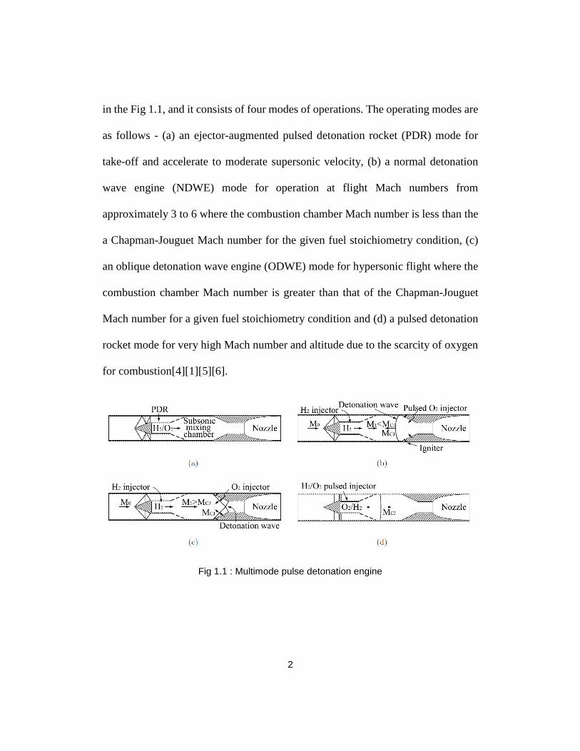
2
in the Fig 11 and it consists of four modes of operations The operating modes are
as follows - (a) an ejector-augmented pulsed detonation rocket (PDR) mode for
take-off and accelerate to moderate supersonic velocity (b) a normal detonation
wave engine (NDWE) mode for operation at flight Mach numbers from
approximately 3 to 6 where the combustion chamber Mach number is less than the
a Chapman-Jouguet Mach number for the given fuel stoichiometry condition (c)
an oblique detonation wave engine (ODWE) mode for hypersonic flight where the
combustion chamber Mach number is greater than that of the Chapman-Jouguet
Mach number for a given fuel stoichiometry condition and (d) a pulsed detonation
rocket mode for very high Mach number and altitude due to the scarcity of oxygen
for combustion[4][1][5][6]
Fig 11 Multimode pulse detonation engine
3
12 Detonation Physics and Chapman ndash Jouguet condition
A detonation wave is a complex oscillating three-dimensional cellular structure
consisting of a shock followed by an induction zone with a coupled reaction region
where the products are accompanied by a rapid release of energy As the detonation
wave propagation is supersonic in nature the reactants upstream are not affected
until the flow comes in contact with the detonation wave front As the shock passes
through the reactants it compresses heats and ignites the mixture resulting in
combustion zone propagating with the velocity of the shock The shock wave is
coupled with the reaction zone triple point transverse wave and shear layer as
shown in the Fig 12 (ab) [4][6][1][2][3] Consider a detonation wave propagating
in a tube filled with a combustible mixture that is closed at one end and opened at
the other The detonation is initiated at the closed end by a high enthalpy source
and the shock wave moves at the velocity of the detonation wave Vdet relative to
the gas chamber The thermodynamics of the process is given by T-S diagram as
shown in Fig 13
4
Fig 12 (ab) schematics of detonation
Fig 13 shows the difference between the constant pressure combustion (Brayton
cycle) constant volume combustion (Humphrey cycle) and detonation cycle The
stage 0 -1 known as the pre-compression is mandatory for a Brayton cycle but for
detonation the leading shock provides the necessary pressure rise to sustain the
combustion
5
Fig 1 3 T-S diagram for different combustion model
This complex concept of detonation is explained by two relatively simple
theoretical model The Chapman-Jouguet (CJ) and Zeldovich-von Neumann-
Doumlring (ZND) models The first theory of detonation was proposed by Chapman in
1899 and followed by Jouguet in 1905 In this theory it is assumed that the chemical
reaction takes place instantaneously inside the shock and the reaction zone length
shrink to zero as shown in Fig 14 The products are assumed to flow at a local sonic
velocity relative to the shock which is called as the Chapman ndash Jouguet condition
6
In this case the velocity of the products can be obtained by the one-dimensional
conservation equation of mass momentum and energy coupled with the chemical
reaction
Fig 14 Chapman ndash Jouguet Detonation model
An improved and more modern theory that takes into the account the effect of the
finite rate chemical reactions was originated from the work of Zeldovich von
Neumann and Doering in 1940rsquos which was later named as the ZND theory This
model of detonation is assumed to have a strong shock wave that is been coupled
to a reaction zone where a fuel and oxidizer mixture is compressed by the leading
shock and is rapidly burned which releases energy that is utilized to sustain the
propagating shock The leading shock travels at the detonation velocity and the
strength of the shock depends on the detonation velocity In this the reaction zone
is divided into two regions namely an induction zone and the heat addition zone
In the induction zone the reaction is delayed due to the finite time required to initiate
the chemical reaction The energy is released in the heat addition zone after the
7
reaction begins From Fig 15 A pressure spike is observed in the induction zone
and it is referred as the Von Neumann pressure spike [2][4][3]
Fig 15 Variation of Pressure and temperature in ZND Detonation
The concept of highly energetic detonation phenomena can be applied to the
propulsion system One such concept of engine is the pulsed detonation engine
(PDE) that was first introduced during the late 1940rsquos The ideal advantage of PDE
over the engine that follows a Brayton cycle is the high thermodynamic efficiency
thatrsquos possible to achieve by controlled combustion through detonation cycle Fig
16 represents the concept of a PDE with a nozzle at the end to expand the
combusted gas A generic PDE cycle consist of four different steps (a) filling of
8
fuel-oxidizer mixture (b) initiating the detonation (c) detonation propagation and
(d) purging of the burned gas in a blowdown process
Fig 16 Pulsed detonation engine cycle
The PDE cycle begins with the detonation chamber being filled with the fuel-
oxidizer mixture through the valve opening In the Fig 16 p0 and p1 are the ambient
and mixture pressure respectively As the detonation velocity is higher than the
velocity of fuel-oxidizer velocity during the filling process the detonation is
initiated before the mixture reaches the end of the chamber using an ignitor An
unsteady expansion wave is generated behind the detonation wave as it propagates
through the combustion medium which explains the pressure of the burned gas
being less than the Von Neumann pressure[6][7][16] An ideal detonation wave
9
will propagate at the Chapman Jouguet (CJ) velocity for the given mixture initial
condition As soon as the detonation exits the chamber a blowdown process is
started due to the pressure difference across the exit plane of the chamber which is
then followed by a purging process thatrsquos basically injecting relatively cool air into
the chamber to clear out the burned gas and to cool the chamber in order to prevent
auto-ignition of the fresh fuel-oxidizer mixture that gets injected in the following
cycle
13 Thermodynamics
In order to understand the detonation process a detailed analysis of
thermodynamics is needed For the analysis a steady state control volume of a
detonation is considered that is shown in the Fig 17 By applying the continuity
momentum and energy equation with a fluid behaving as an ideal gas to the control
volume represented in the Fig 17 gives the following [17][4][14]
Fig 17 Flow properties across a detonation
10
1205881 lowast 1199061 = 1205882 lowast 1199062 (11)
1199011 + 120588111990612 = 1199012 + 12058821199062
2 (12)
11988811990111198791 +1
21199061
2 + 119902 = 11988811990121198792 +1
21199062
2 (13)
1199011 = 120588111987711198791 (14)
1199012 = 120588211987721198792 (15)
In these equations the heat addition because of the chemical reaction is accounted
by the term q The total enthalpy of the mixture is defined as h = cpT +ho In the
above equation the heat addition is accounted by the term q = h2 ndash h1
The equation that relates the thermodynamics properties across the discontinuity is
obtained by simplifying the Rankine ndash Hugoniot equation [2][3][17]
ℎ2 minus ℎ1
= 1
2 (
1
1205882minus
1
1205881) (1199012 minus 1199011)
(16)
11
which is simplified to
1
120574 minus 1 (11990121205922 minus 11990111205921) minus
1
2 (1199012 minus 1199011)(1205922 + 1205921) minus 119902 = 0
(17)
The Rankine ndash Hugoniot curve is represented in the Eq 17 It is important to plot
the Hugoniot equation in terms of (p υ) as total enthalpy is a function of (p ρ) and
the solution lies in this plane regardless of the flow velocity The Rankine ndash
Hugoniot curve is given in the Fig 18 (a) and (b) The line that is tangential to the
Rankine ndash Hugoniot curve is the Rayleigh line representing mass flux from the Eq
18
(1199012 minus 1199011)
(11205882
minus 11205881
) = minus
(18)
12
Fig 18 (a) Rankine ndash Hugoniot curve
Fig 18 (B) Rankine ndash Hugoniot curve to calculate von Neumann pressure spike
13
The point on the Hugoniot curve where the Rayleigh line is tangential to each other
is known as the Chapman ndash Jouguet (CJ) point Theoretically there are two CJ
points on a Hugoniot curve the upper CJ point (CJu) and the lower CJ point (CJl)
They are located respectively where the Raleigh line is tangential to the Hugoniot
curve on the detonation and deflagration branch The Hugoniot curve is divided
into five regions and is represented in the Table 11
Regions in Hugoniot Characteristics Burned gas velocity
Region 1 (A - B) Strong Detonation Subsonic
Region 2 (B - C) Weak Detonation Supersonic
Region 3 (C -D) The relation is not satisfied
Region 4 (D - E) Weak deflagration Subsonic
Region 5 (E and F) Strong deflagration supersonic
Table 11 ndash Regions in Hugoniot curve
Starting from region 3 any region upstream and downstream of the given region
satisfies the Rayleigh and Hugoniot relations that is been represented in the Eq 18
and Eq 17 respectively The region 3 does not represent any real solution for the
equation In this case between the region 2 and 4 no valid Rayleigh lines could be
drawn
14
The regions 1 and 2 corresponds to strong and weak detonation regions
respectively the region 4 and 5 represents the weak and strong deflagration
respectively In case of a detonation the gas dynamic properties of the fluid are
needed to determine the burned gas propagating speed thatrsquos independent of the
actual structure of the wave This discovery was initially made by Chapman and
Jouguet in the early 20th century It was Chapman who postulated that solution
points are when the Rayleigh line is tangential to the Hugoniot curve
The region 1 represents the conditions required for a strong detonation In this case
the burned gas will be of subsonic Mach number referenced to the local
temperature The gas behind the detonation will still follow up the detonation at CJ
velocity The region 2 represents the conditions for a weak detonation with burned
gas having a supersonic Mach number The region 4 and 5 represents the condition
to have a deflagration In case of deflagration the propagating speed is determined
by the transport properties of the gasses The region 4 is a weak deflagration and
the region 5 is a strong deflagration [4][3] The conditions at the point B is the
upper C-J point and the point E represents the lower C-J point
By calculating the entropy at the C-J points for a given stoichiometry It can be
observed that a higher entropy is achieved for the conditions corresponding to the
15
upper C-J point And a lower entropy value is obtained from the conditions that
corresponds to the lower C-J point
The major importance of C-J theory is to obtain the detonation flow properties The
C-J wave propagation speed was experimentally measured by Winterberger in 2004
and found to be within a range of 2 with the theoretical CJ theory The detonation
temperature is given by [3][17]
119879119889 = 120574119889
2120574119889 + 1 (
119862119901119906
119862119901119889 119879119906 +
119902
119862119901119889)
(19)
The detonation velocity for a real gas Vd is represented as
119881119889 = radic2(120574119889 + 1)120574119889 119877119889 (119862119901119886
119862119901119889 119879119906 +
119902
119862119901119889)
(110)
When the downstream fluid is of CJ condition then the Eq (110) can be written as
119881119862119869 = 120588119862119869
120588119906 radic120574119862119869 119877119862119869 119879119862119869
(111)
16
Chapter 2
GOVERNING EQUATIONS
To simulate of a flow with a reacting gas mixture the chemical reaction between
the gases need to be modeled together with the fluid dynamics For example in the
case of detonation or combustion the basic equations of the reactive flow are the
conservation of the mass energy and momentum along with the change in
composition of gas mixture due to reaction[4][5][17]
21 Reactive Euler equation
Ignoring viscosity heat transfer diffusion radiation and body forces the governing
equation for a compressible reactive flow are the reactive Euler equation
[4][17][25] The axisymmetric reactive Euler equation are used for modeling the
PDEs combustion chamber In actuality the detonation is characterized by a three-
dimensional cellular structure which these equations lack the physical makeup to
capture Since the research is to identify the gas dynamic of various flow features
the axisymmetric model representation will work for our case The reactive Euler
equation are given by
17
120597119928
120597119905+
120597119917
120597119909+
120597119918
120597119903+ 119919 = 119934
(21)
where the state vector Q flux vector in the x-direction F flux vector in r-direction
G axisymmetric term H and the species source term W are defined as
119928 =
[
120588120588119881119909
120588119881119903
120588119864120588119884119894 ]
119917 =
[
120588119894119881119909
1205881198811199092 + 119901
120588119881119909119881119903(120588119864 + 119901)119881119909
120588119881119909119884119894 ]
119918 =
[
120588119894119881119909
120588119881119909119881119903
1205881198811199032
(120588119864 + 119901)119881119903120588119881119903119884119894 ]
119919 =1
119903
[
120588119894119881119903
120588119881119909119881119903120588119881119903
2
(120588119864 + 119901)119881119903
120588119881119903119884119894 ]
119934 =
[ 0000119877119894]
(22)
18
Here ρ V E and p are the density velocity total energy per unit mass and the
pressure of the fluid respectively Ri corresponds to the net rate of production of an
individual species due to chemical reaction and i = 1hellip Ns where Ns is the number
of species The Eq 22 inherits gas dynamics and chemical reaction coupling that
is required for modeling a self-sustained detonation
The assumptions made in the 2-D reactive Euler equations are the external forces
like gravity are negligible as the force is small in a hypersonic combustion but not
in a low-speed combustion The mass diffusion due to thermal and pressure
difference and the heat transfer due to radiation and concentration difference known
as the Dufour effect is assumed to be negligible
The 1st term represents the continuity term for the flow and gas dynamics property
The last row of the source terms in Eq (22) represents the species continuity in the
mixture that is valid for a finite reaction rate The 2nd 3rd and 4th row corresponds
to the momentum in the x-direction and r-direction and the energy equation
respectively And the pressure and temperature diffusivity terms are neglected since
they are usually exceedingly small The Eq (22) describes large class of
combustion problems that are generally quite complex
19
We introduce a preconditioned pseudo-time-derivative term in Eq (21) as
120575
120575120591 int119928 119889119881
119881
+ ∮[119917 + 119918] 119889119860 + int 119919 119889119881 = 120575
120575119905 int119934 119889119881
119881119881
(23)
where t denotes the physical time step and τ denotes the pseudo-time used in the
time-marching procedure When τ tents to infinity Eq (13) will be the same as Eq
(11) The time-dependent term in Eq (13) is discretized in an implicit fashion by
a Second-order accurate backward difference in time The dual time formulation
is written in semi-discrete form as follows
[Γ
∆120591+
1205980
∆119905 120575119934
120575119928] + ∮[119917 + 119918] 119889119860
+ int 119919 119889119881 = 1
∆119905(1205980119934
119896 minus 1205981119934119899 + 1205982119934
119899minus1) 119881
(24)
22 Thermodynamics Relation
Species and Mixture The gas mixture as a whole is an ideal gas and the
properties are functions of both temperature and pressure due to rapid change in
chemical composition In terms of individual species they are considered to be
thermally perfect gas [6][10][13]
20
119888119901 119894119904 119886 119891119906119899119888119905119894119900119899 119900119891 119879119890119898119901119890119903119886119905119906119903119890 (25)
119888119907 119894119904 119886 119891119906119899119888119905119894119900119899 119900119891 119879119890119898119901119890119903119886119905119906119903119890 (26)
The enthalpy and internal energy of species are given by
ℎ119894 = ℎ119894119891
+ int 119888119901119894 119889119905119879
1198790
(27)
119890119894 = ℎ119894119891
+ int 119888119907119894 119889119905119879
1198790
(28)
where ℎ119894119891 is the heat of formation of the ith species at a reference temperature
29815K also known as the heat of formation and is normally obtained from the
thermodynamics database
The above equations Eq (27) and Eq (28) are standard form for an arbitrary ndash
order polynomial The general form of the molar specific heat works with the
thermodynamic data in the form used in the NASA CEA In this case seven
coefficients are needed for polynomial function of temperature This is expressed
in the following form
119862119901119894
119877= 1198861119879
minus2 + 1198862119879minus1 + 1198863 + 1198864119879
1 + 11988651198792 + 1198866119879
3 + 11988671198794
(29)
21
The molar enthalpy is given as
119867119894
119877119879= minus1198861119879
minus2 + 1198862119879minus1119897119899119879 + 1198863 + 1198864
119879
2+ 1198865
1198792
3+ 1198866
1198793
4+ 1198867
1198794
5
+ 1198868
119879
(210)
The entropy of the species is calculated by
119878119894
119877= minus1198861
119879minus2
2minus 1198862119879
minus1 + 1198863119897119899119879 + 1198864119879 + 1198865
1198792
2+ 1198866
1198793
3+ 1198867
1198794
4
+ 1198869
(211)
The coefficients a1 to a9 in Eq 29 ndash 211 are obtained from the thermodynamics
database that takes into account the rotational and vibrational energy of the species
over a temperature range from 200 K to 6000 K From the above equation Eq (28)-
(211) the specific heat and enthalpy of the species per unit mass are a function of
temperature and are given by
119888119901119894 = 119877
119882119894 119862119901119894
(212)
ℎ119894 = 119877119879
119882119894 119867119894
(213)
The specific heat at constant volume and internal energy is given by
22
119888119907119894 = 119888119901119894 minus119877
119882119894
(214)
119890119894 = ℎ119894 minus 119877119879
119882119894
(215)
By taking the summation of i from 1 to Ns the above four equations will provide
the thermodynamic properties of the fluid such as the specific heat at constant
pressure enthalpy specific heat at constant volume and entropy
Ideal gas equation The equation of state for an ideal gas is given by
119875 = sum120588119877119894119879
119873119904
119894=1
(216)
where
119877119946 = 119877
119882119946
(217)
where R is the universal gas constant (8314 J mol K) and ρ is the total density of
the mixture
The speed of sound is given by
119914 = radic120574119877119879 = radic120574119875
120588
(218)
Where γ is the ratio of specific heat
23
23 Chemical Kinetics
A detailed and a stable chemical model is necessary for the source term in Eq 22
is necessary in order to create an accurate numerical model of detonation Due to
rapid chemical reaction in the case a detonation right behind the shock discontinuity
creates stiffness in source terms To overcome the stiffness in the source term due
to chemical reaction and the chemical non-equilibrium the entire source terms need
to be solved simultaneously
Chemical Reaction Mechanism Taking the stoichiometry reaction of hydrogen-
air the balanced chemical reaction equation is given as
21198672 + (1198742 + 3762 1198732) rarr 21198672119874 + 3762 1198732 (219)
To attain this reaction a series of elementary reaction which represented in a step
by step sequence by which the overall reaction takes place is named as the chemical
reaction mechanism The reaction mechanism consists of the information regarding
reaction rate third body and pressure depended reaction that represents the accurate
reaction mechanism as a whole Combining all the elementary reactions will give
24
rise to the detailed reaction with lower chemical stiffness that will be used for the
numerical simulation of detonation wave
The hydrogen-air mechanism is represented in various detailed levels from a single
step two steps to a detailed 268 step reaction mechanism [11] In this study a 11
species and 23 step hydrogen-air model thatrsquos shown in Table1 is employed as a
good representation of the hydrogen-air mechanism for the required operating
condition
The general form of the chemical reaction is written in a compact form as
sum120592119894119895prime
119873119904
119894=1
119872119894 harr sum120592119894119895
119873119904
119894=1
119872119894
(220)
where i and j are the number of species and number of reactions respectively In
this relation 120592119894119895prime and 120592119894119895
represents the stoichiometric coefficient of the reactants
and products respectively
From the elementary reactions the net rate of production of a given species is given
by
119894 = sum(120592119894119895 minus 120592119894119895
prime )
119873119903
119895=1
119896119891119895 prod[119872119894]120592119894119895
119873119904
119894=1
minus 119896119887119895 prod[119872119894]120592119894119895
prime
119873119904
119894=1
(221)
25
In this relation the forward reaction rate is given by 119896119891119895 for the jth reaction which
is obtained through the Arrhenius equation [11][10][17]
119896119891119895 = 119860119903 119879119899 119890minus
119864119903119877119879
(222)
and the backward reaction rate is given by
119896119887119895 = 119896119891119895
119896119888119895
(223)
where
119896119888119895 = 119896119901119895 (119875119886119905119898
119877119879)
sum (120592119894119895 minus 120592119894119895
prime )119873119904119894=1
(224)
119896119901119895 = 119890119909119901 [sum(120592119894119895 minus 120592119894119895
prime ) (119878119894
119877minus
119867119894
119877119879 )
119873119904
119894=1
]
(225)
The term 119860119903 is the pre-exponential factor n is the temperature exponent and 119864119903 is
the activation energy The values are given in Table 21 for hydrogen-air reaction
The backward reaction rate 119896119887119895 in Eq 223 is determined by the forward reaction
rate and the equilibrium constant The equilibrium constant 119896119888119895 is determined from
the Eq 224 and Eq 225 119875119886119905119898 represents the sea level atmospheric pressure and
the terms 119867119894
119877119879 and
119878119894
119877 are derived from the Eq 210 and Eq 211 respectively
26
REACTION MECHANISM A
mole-cm-sec-K b
E
calmole
H2 + O2 lt=gt OH + OH 170E+13 0 47780
OH + H2 lt=gt H2O + H 117E+09 13 3626
O + OH lt=gt O2 + H 400E+14 -05 0
O + H2 lt=gt OH + H 506E+04 267 6290
H + O2 + M lt=gt HO2 + M
H2O enhanced by 186
H2 enhanced by 286
N2 enhanced by 126
361E+17
-072
0
OH + HO2 lt=gt H2O + O2 750E+12 0 0
H + HO2 lt=gt OH + OH 140E+14 0 1073
O + HO2 lt=gt O2 + OH 140E+13 0 1073
OH + OH lt=gt O + H2O 609E+08 13 0
H + H + M lt=gt H2 + M
H2O enhanced by 00
H2 enhanced by 00
100E+18
-10
0
H + H + H2 lt=gt H2 + H2 920E+16 -06 0
H + H + H2O lt=gt H2 + H2O 600E+19 -125 0
H + OH + M lt=gt H2O + M
H2O enhanced by 50 160E+22 -2 0
H + O + M lt=gt OH + M
H2O enhanced by 50 620E+16 -06 0
O + O + M lt=gt O2 + M 189E+13 0 -1788
H + HO2 lt=gt H2 + O2 125E+13 0 0
HO2 + HO2 lt=gt H2O2 + O2 200E+12 0 0
H2O2 + M lt=gt OH + OH + M 130E+17 0 45500
H2O2 + H lt=gt HO2 + H2 160E+12 0 3800
H2O2 + OH lt=gt H2O + HO2 100E+13 0 1800
O + N2 lt=gt NO + N 140E+14 0 75800
N + O2 lt=gt NO + O 640E+09 1 6280
OH + N lt=gt NO + H 400E+13 0 0
Table 21 Reaction mechanism of Hydrogen -air
27
Third Body Reactions These reactions tend to appear in the detailed reaction
mechanism when the reactants or products is having higher bonding energy An
example for a third body reaction is
119867 + 1198742 + 119872 harr 1198671198742 + 119872 (226)
where M the third body could be 11986721198741198672 1198732 In this the energy released from the
formation of 1198671198742 from 119867 and 1198742 is carried out with the help of the third body In
the backward reaction the third body provides the required amount of energy to
break the bond in 1198671198742 to give rise to 119867 and 1198742[4][10][6] The molar concentration
with the third body efficiency is given by
119883119894 = sum120572119894119895[119872119894]
119873119904
119894=1
(227)
where the 120572119894119895 is the third body efficiency The rate of mass production Eq 221
becomes
119894 = sum(120592119894119895 minus 120592119894119895
prime )
119873119903
119895=1
[119883119894] 119896119891119895 prod[119872119894]120592119894119895
119873119904
119894=1
minus 119896119891119895 prod[119872119894]120592119894119895
prime
119873119904
119894=1
(228)
28
Chapter 3
NUMERICAL METHOD
In a chemically reacting flow there are several numerical difficulties that have to
be taken into account In a reactive flow the species continuity equations are
coupled with the governing equations that have to be solved simultaneously Due
to a wide range of time scales in the flow that leads to numerical stiffness that has
to be compensated for and there is physical complexity due to coupling of fluid and
chemical kinetics In the case of detonation due to the discontinuity and small-time
steps an extremely fine grid spacing is required to model the discontinuity across
the detonation
31 Density-based solver
In the governing equations as the flow and chemical kinetics are coupled with each
other they have to be solved simultaneously The density-based solver solves the
governing equation of continuity momentum energy and species transport
simultaneously in a coupled manner as in the flowchart described in Fig 31 Since
the governing equations are nonlinear several iterations of the solution loops have
to be performed before obtaining the converged solution [12][13]
29
Fig 31 Solution method in a density-based solver
The density-based solver discretizes the non-linear equation into a linearized form
to have a system of equations for a dependent variable in each cell The resulting
linear variables can be solved by two methods explicit and implicit In this case
the density based implicit solver is chosen In the implicit solver the governing
equations are linearized implicitly with respect to all the dependent variables in the
set This results in a linear system of equation with N equations for each cell in the
30
domain that has to be solved simultaneously where N is the number of coupled
equations in the governing set of equations For example in terms of continuity
momentum in x-direction and y-direction and energy the unknowns are p u v
and T By simultaneously solving the unknowns using a block Algebraic Multi-
Grid (AMG) solver this gives an implicit approach to solve the unknown variables
at the same time
32 Discretization and Solution
A finite volume formulation was used to convert the transport properties to an
algebraic form in the two-dimensional reactive Euler equation given in Eq 21
which is expressed as follows
int119876 119889119881
119881
+ ∮120583 120601 119889119860 = int119878 119889119881
119881
(31)
where V is the control volume A is the surface area 120583 is flux term defined as
120583 = 119865119894 + 119866119895 (32)
and 120601 is the normal unit vector defined as 120583 = 119889119909119894 + 119889119903119895
31
33 Spatial Discretization
Monotone upstream ndash centered schemes (MUSCL) In order to achieve third
order accuracy in space the MUSCL scheme [21][18] was employed The values at
face υf are been interpolated from the cell center values This is accomplished by
using upwind schemes The upwinding means the face values υf is derived from the
quantities of the cell upstream in the direction normal to the velocity Monotone
upstream-centered schemes for conservation laws (MUSCL) were used for the flow
spatial discretization The MUSCL is a created by blending the central difference
scheme and second-order upwind scheme The formulation of the MUSCL scheme
is given by
120592119891 = Θ120592119891119862119863 + (1 minus Θ)120592119891119878119874 (33)
where 120592119891119862119863 is obtained from the central difference scheme as follows
120592119891119862119863 = 1
2 (1205920 + 1205921) +
1
2 (nabla1205920 1206010119891 + nabla1205921 1206011119891)
(34)
where 0 and 1 terms represent the cell share faces The nabla terms are the reconstructed
gradient at cell 0 and 1
32
The term 120592119891119878119874 is obtained from the second order upwind stream The quantities at
the cell faces are computed using multidimensional reconstruction approach
[12][13][18] The higher order accuracy is achieved by Taylor series expansion of
the cell centered solution It is computed as follows
120592119891119878119874 = 120592 + nabla120592 ∙ 120601119891 (35)
where υ and nabla120592 are the cell center values and the gradient of the cell center values
respectively in the upstream 120601 represents the displacement vector from the
upstream of the cell face centroid The gradient term is spatially discretized by
using second order upwind scheme is the Green-Gauss cell-based which is
discussed below
Green-Gauss Theorem The gradients used for computing values of a scalar term
120601 at the cell faces center[21][18][20] The Green ndash Gauss theorem is described as
(nabla120592)119888 = 1
119907 sum120601119891 119860119891
119891
(36)
where 120601 is referred as the gradient of the scalar properties at cell center c and 120601119891
represents the value of 120601 at the cell face center is expressed as
120601119891 = 1206011198880 + 1206011198881
2
(37)
where 1206011198880 and 1206011198881 are the values at the neighboring cell centers
33
Advection Upstream Splitting Method (AUSM) The convective fluxes at each
cell F and G in Eq (31) are approximated by the flux vector splitting scheme
known as Advection upstream splitting method (AUSM) This was introduced by
Liou and Steffen in 1993 [21][19][18] This scheme first computes a cell interface
Mach number based on the characteristic speed from the adjacent cell The interface
Mach number is then used to determine the upwind extrapolation for the
convection part of the fluxes The pressure terms are obtained by splitting of Mach
number A generalized Mach number-based convection and pressure terms were
proposed by Lion [21[19][18] This provides the resolution for the shock
discontinuity and damps the oscillations at stationary and moving shocks The
scheme is expressed as follows
119865 = 119898119891120592 + 119875119894 (38)
where 119898119891 represents the mass flux through the interface The mass flux is calculated
from left to right of the interface by using the forth order polynomial
Temporal discretization For a transient simulation the governing equations Eq
(21) and Eq (22) must be discretized in both space and time This involves the
discretization of the terms at every time step ∆119905 The generic expression for the
scalar quantities with respect to time step is given by
34
120575120592
120575119905= 119865(120592)
(39)
The time derivative was calculated using a backward difference second-order
discretization is expressed as
119865(120592) = 3120592119894+1 minus 4120592119894 + 120592119894minus1
2Δ119905
(310)
where υ is the scalar quantity i is the value at the current time step i+1 is the value
at t + Δ119905 and i-1 is the value at t ndash Δ119905
An implicit time integral was selected because the scheme is unconditionally stable
with respect to time step size The downside of an implicit scheme is if the solver
was not optimized then the runtime will increase drastically The formulation to
evaluate F(υi+1) is given by
120592119894+1 minus 120592119894
Δ119905= 119865(120592119894+1)
(311)
where
120592119894+1 = 120592119894 + Δ119865(120592119894+1) (312)
High order term relaxation The importance of high order terms is to improve
the start-up and the general solution behavior of flow simulations when a higher
35
order spatial discretizationrsquos were used This also prevents convergence stalling in
many cases which leads to numerical instabilities The HOTR is used to reduce the
interaction of numerical instabilities in an aggressive solution The HOTR is written
as the first order scheme plus the additional terms from the higher order schemes
The Relaxation factor for the higher order scheme is described as follows
120593119894+1 = 120593119894 + 119891(120593119894+05 minus 120593119894) (313)
where 120593 is a generic formulation for any terms from single to higher order and 119891
is the under-relaxation term
Algebraic Multigrid (AMG) In this case a F ndash cycle multigrid was selected F-
cycle is essentially a combination of V and W cycles as described below in Fig 32
119953119955119942 119956119960119942119942119953 rarr 119955119942119956119957119955119946119940119957 rarr 119934 119940119962119940119949119942 rarr 119933 119940119962119940119949119942 rarr 119953119955119952119949119952119951119944119938119957119942 rarr 119953119952119956119957 119956119960119942119942119953
Fig 32 F ndash cycle multigrid solver
where the restriction and propagation are used based on the additive correction
strategy [21][18]
36
34 Boundary Conditions
Pressure Inlet In the case of a compressible inlet the pressure inlet evaluates the
isentropic flow relations using ideal gas relations The input total pressure P0 and
the static pressure Ps in the adjacent cells are related as
1198750 + 119875119900119901
119875119904 + 119875119900119901= (1 +
120574 minus 1
2 1198722)
120574120574minus1
(314)
where
119872 = 119881
radic120574119877119879119904
(315)
The density and the temperature at the inlet plane is from the ideal gas law that is
given as follows
120588 = 119875119904 + 119875119900119901
119877119879119904
(316)
1198790
119879119904= 1 +
120574 minus 1
2 1198722
(317)
where op is the operating condition The individual velocity components at the inlet
are derived using the direction vector components
37
Pressure Outlet This outlet condition extrapolates the values at the exit from the
interior of the domain The extrapolation is carried out by using the splitting
procedure based on the AUSM scheme [4][18][20][21]
Symmetry The geometry is taken to be 2-D axis-symmetric There are no flux
terms across the boundary with zero normal velocity component
35 Computational Resources
Generally a chemically reactive flow solution requires an extended amount of
computational time and resources are required in order to obtain a converged and
accurate solution due to the complexity in the problem The run-time of the
numerical simulation of a reactive flow is reduced by using multiple CPUrsquos with
optimum number of cores and nodes Extensively increasing the processor number
will also lead to increase in run-time as the commutation time among the processor
cores are higher than the communication between the nodes for an efficient
performance minimum communication among the processors has to be maintained
Stampede 2 from Texas Advanced Computing Center (TACC) [22][23] was
utilized remotely for running the simulations The TACC was accessed through
windows secured copy (WinSCP) protocol The flowchart in Fig 33 represents the
process involved in accessing fluent in TACC
38
Fig 33 Accessing Fluent in TACC
39
Chapter 4
CHEMISTRY MODELING
The stability of the chemical reaction plays a vital role in the detonation
combustion In order to model the chemical kinetics chemked was used which runs
Chemkin III solver in the background The results obtained from chemked is
validated by comparing with the NASA CEA results [12][13][10]
The formulas used to calculate the reaction rate is explained in section 23 The
input file for the Chemked is in the Chemkin III format [10] and was modified
according to the required case The input file for the chemical kinetics solution for
the detonation in Chemkin format is provided in the APPENDIX along with the
thermodynamic properties of the materials in the reaction which was obtained from
NASA-CEA [12] and GRI mech [13][10]
The rate change of mole fraction with respect to time is compared with THYi [20]
and Chemkin III A Fortran chemical kinetics package for analysis of gas-phase
chemical and plasma kinetics [10] with the following initial conditions of pressure
as 1 atm and temperature as 1500 K The initial mole fraction of hydrogen is 0296
oxygen is 0148 nitrogen is 0556 which corresponds to the stoichiometry for
40
hydrogen-air reaction [4][6][20] The hydrogen-air reaction mechanism considered
here is a 11 species and 23-step reaction model which has an operating range from
400 K to 6000 K This reaction takes into consideration of all the quantum modes
of energy in the molecule as the vibrational mode tends to dominate above 2800 K
for Nitrogen molecule which is near to the detonation temperature of hydrogen-air
for the given operating condition
Increasing the number of chemical steps in the model will provide a detailed
separation of the induction and reaction zone in the detonation But while
considering the global scale of the problem the complexity of the solution will
increase which in turns increases the runtime of the simulation So compromises
had to be made in selecting an appropriate reaction model for the hydrogen-air
reaction without losing the details that are required for simulating a detonation For
the above mentioned initial condition the Fig 41 provides the rate change of mole
fraction of the species with respect to time The graph was generated using MatLab
from the data that been obtained from the Chemked solver
41
Fig 41 Time variation of mole fraction for 23 step and 11 species hydrogen -air
reaction p = 1 atm and T = 1500 K
42
Fig 42 Temperature variation with respect to time
Fig 43 Pressure variation with respect to time
43
Chapter 5
GEOMETRY AND GRID STUDY
In this chapter we discuss about the geometry and the grid study of the 2-D
axisymmetric combustion chamber for unsteady detonation-simulation And also
the methods that are used to validate the boundary condition in order to obtain the
required results in a cold flow and the necessary steps that have been carried out
for a grid independence study for the given geometry to capture the detonation C-J
condition by checking the pre and post-shock properties along with the C-J
condition the NASA CEA [12][13]
The combustor geometry is a two-dimensional axis-symmetric combustion
chamber consisting of a wedge followed by a shock cancelation zone The wedge
angle was chosen after a flow study carried out on different wedge angles for
different modes of detonation done by Hui ndash Yuan Fan [6][4][20] The wedge angle
of 15o is selected because this lies in a complex region where the initiation of both
oblique and normal detonation wave is made possible by changing the inlet
condition of the combustion chamber The sketch of the geometry is given in Fig
51
44
Fig 51 Two ndash Dimensional combustion chamber
SOD shock tube problem This problem is being taken as a base reference in order
to check if the given initial conditions and the solver for the given geometry with
the following structured grid size are able to capture the shock along with the pre
and post-shock conditions The geometry used for the SOD problem with the grid
used is displayed in Fig 52 The initial condition of the region 4 and region 1 in the
shock tube are given as follows
(120588 120592 119901) = (10 010) 119894119891 0 lt 119909 lt 5
(0125 0 01) 119894119891 5 lt 119909 lt 10
(51)
45
Fig 52 SOD Shock tube problem (SOD) geometry
The plots in Fig (53) (54) (55) represents the ρυ p at a given time are expressed
in a was it been expected From this it can be inferred that the given geometry with
the following grid size of 009 mm with a time step of 10-5 sec is capable of
capturing the shock with the above-mentioned boundary condition
Fig 53 Density along x-axis
46
Fig 54 velocity along x-axis
Fig 55 pressure along x-axis
47
Grid independence study The grid independence study is important for modeling
a detonation as the detonation wave speed is strongly dependent on the grid spacing
[6][20]and this also helps in analyzing an appropriate grid size so the detonation is
not inadequately resolved which leads to divergence and improper results or highly
resolved which increases the total time but with just 1 or 2 variations in the
required output For the grid independence study a model which measures 10 x
1449 cm2 in length and height was created with a grid sizing of 01 009 007
003 mm The entire geometry was initialized with the stoichiometric hydrogen-air
mixture with was solved by the chemical kinetics that has been discussed in chapter
4 with the pressure of 1 atm and temperature of 700 K The CJ conditions and
detonation parameters for stoichiometric hydrogen-air mixture at the given initial
condition is obtained from NASA-CEA which are 119901
1199011 is 6631 and
119879
1198791 is 4291 119901
and 119879 are the post-detonation pressure and temperature were 119901 equates to 671900
pa and 119879 equates to 300347 K [12][13] To initiate detonation in the tube a high
enthalpy region of pressure 40 atm and temperature 4000 K was patched at the
closed end of the tube that has been shown in Fig 56 and the other end is set to be
a pressure outlet to atmosphere condition The Fig 57 58 59 are the graph
comparison for pressure temperature and velocity respectively at a given time
52x10-4 seconds It can be seen that grid size plays an important role in achieving
CJ condition for the given condition and chemical reaction As it can be observed
48
from the Fig (57)(58) grid size 003 mm is the preferred grid size for capturing the
detonation
Fig 56 Initial pressure and temperature contour for grid study
49
Fig 57 Pressure along x-axis at time 45 x 10-4 sec
Fig 58 Temperature along x-axis at time 45 x 10-4 sec
50
Fig 59 velocity along x-axis at time 45 x 10-4 sec
The fluctuations of values in the Fig 57 ndash 59 are due to the interaction of shear
layer after the detonation cell that is visible in the Fig 511 ndash 513 the oscillations
in the values can be reduced by reducing the grid size or by using an Adaptive Mesh
Refinement (AMR)
51
Fig 510 Detonation propagation in the grid size 003x10-5 m
52
Fig 511 Temperature contour in grid size 003 m x10-5 m
Fig 512 Velocity contour in grid size 003 x10-5 m
53
Fig 513 Numerical schlieren imaging
Fig 514 Mass fraction of H2 O2 H2O
54
The Fig (510) (511) (512) (514) are the representation of pressure temperature
velocity heat of reaction and mass fraction of species (H2 O2 H2O) respectively
for geometry with the grid size of 003 mm The Fig 51 represents the combustion
chamber which was meshed with a grid sizing of 003 x 10-5 m The total number
of cells is 2458464 and nodes is 2462005 The schematic of a two-dimensional
combustion chamber has been described in the Fig 51
55
Chapter 6
RESULTS AND DISCUSSION
The results were analyzed and post-processed using ANSYS CFD-Post
[18][20][22] and the numerical schlieren was created by using paraview In a
simulation of unsteady normal detonation the concept of detonation strength had
to be understood properly As its known that if the detonation incoming Mach
number (M35) is less than the CJ Mach number (MCJ) for the given stoichiometry
condition the detonation wave tends to move upstream in the combustion chamber
and on the other hand if the detonation incoming Mach number (M35) is higher
than the CJ Mach number (MCJ) for the given stoichiometry condition then the
detonation tends to move downstream along with the flow [4][6][15] The above
property of detonation was utilized in order to move the detonation wave upstream
and downstream inside the combustion chamber As the detonation strength
depends on the detonation chamber incoming Mach (M3) the M3 is varied by fixing
the flow inlet properties namely the pressure temperature and velocity to a
particular value in a cycle and varying the mass fraction of the fuel
For the case - I the MCJ equals to 3108 for a stoichiometric hydrogen-air with
pressure 101325 Pa and temperature 700 K as initial condition The combustion
chamber incoming Mach number 35 will have M35 equivalent to 2669 due to the
56
presence of oblique shock formed by the wedge With M35 being less that MCJ the
detonation wave would propagate upstream If the fuel is turned off that would
make the incoming flow to purge the combustion chamber and would convert the
propagating detonation wave to a propagating blast wave This blast wave will
eventually die off with no fuel in the incoming flow The problem faced in this
scenario was the length required by the blast wave to reduce in strength and die off
was longer than the length anticipated which was solved by changing the incoming
flow equivalence ratio to 05 instead of purging the chamber The MCJ equals to
282 for an equivalence ratio of 05 with the same initial conditions The change in
γ makes the combustion chamber incoming Mach number to 38 that with have a
M35 equal to 291 The M3 being larger than MCJ the detonation wave will propagate
downstream with the flow This method of NDW will oscillate the detonation wave
inside the combustion chamber and will produce a constant flow properties at the
combustion exit plain
Flow of this chapter is going to be as follows first explaining the different cases
for an unsteady normal detonation wave combustion which provides the cycle
time The cases are varied according to their initial conditions variables namely
pressure temperature and velocity The final part of the chapter is to analyze the
variation in pressure temperature and velocity ratios with respect to time at the exit
57
of the combustion chamber The Table 61 62 63 consists of the initial conditions
for the different cases
Case I
Equivalence ratio Inlet condition Time steps elapsed time
(sec)
Equivalence ratio - 1
Pressure ndash 101325 pa
Temperature ndash 800 K
Mach number ndash 35
Velocity ndash 2304874 msec
0 to 1500
15 x 10-4
Equivalence ratio ndash 05
Pressure ndash 101325 pa
Temperature ndash 800 K
Mach number ndash 38
Velocity ndash 2303281 msec
1500 to 7000
55 x 10-4
Equivalence ratio ndash 1
Pressure ndash 101325 pa
Temperature ndash 800 K
Mach number ndash 35
Velocity ndash 2304874 msec
7000 to 8000
1 x 10⁻⁴
Equivalence ratio ndash 05
Pressure ndash 101325 pa
Temperature ndash 800 K
Mach number ndash 38
Velocity ndash 2303281 msec
8000 to 11500
35 x 10-4
Equivalence ratio - 1
Pressure ndash 101325 pa
Temperature ndash 800 K
Mach number ndash 35
Velocity ndash 2304874 msec
11500 to 12500
1 x 10⁻⁴
Table 61 case I
58
CASE I In this case as mentioned in Table 61 the initial conditions are static
pressure in the combustion chamber is 101325 Pa the static temperature is 800 K
with a Mach number of 35 that gives the velocity in x-axis at the inlet to be 2304
msec the equivalence ratio for this cycle φ is 1 It is necessary to have a similar
flow time step and chemical time step in order to avoid the instabilities This
requires the flow to have a time step of a 10-7 sec which is the appropriate time
step for a detonation with the specified chemical kinetics of hydrogen-air
[2][20][6] In this case the M3 is less than the MCJ which causes the detonation to
propagate upstream The detonation should be made to move downstream before it
crosses the wedge because if the detonation is upstream of the wedge due to the
presence of a strong normal shock in front of the reaction zone which in turn causes
the detonation to propagate upstream no matter what the inlet equivalence ratio is
set The next cycle starts when the equivalence ratio φ is changed to 05 while
maintaining the same inlet pressure temperature and velocity This causes the
Mach number to go up to 38 which makes the M3 to be higher than MCJ A single
cycle time is the addition of first and second stage elapsed time The evolution of the
flow from initiation and propagation of an unsteady detonation wave with respect
to time is shown in the Fig 61 ndash 65
59
Fig 61 Time from 0 to 15 x 10-4sec
60
Fig 62 (ab) Time from 15 x 10-4to 60 x 10-4sec
61
Fig 63 Time from 60 x 10-4to 70 x 10-4 sec
62
Fig 64 Time from 70 x 10-4 to 14 x 10-4sec
63
Fig 65 Time from 14 x 10-4 to 24 x 10-4 sec
64
CASE II The initial conditions and the cycle time is mentioned in Table 62 The
methodology is similar to the CASE 1 but the difference is in the initial conditions
The initial conditions for this case are a static pressure in the combustion chamber
of 506625 Pa which corresponds to a high-altitude flight with a static temperature
of 800 K Mach number of 35 with an equivalence ratio of 1 This equates to a flow
velocity at the combustor inlet of 2304 msec The second cycle of this case starts
when the equivalence ratio is reduced to 05 and the pressure temperature and
velocity are maintained at the same values which increases the flow Mach number
to 379 The propagation of the flow is similar to that of the case I with minor
variation in the cycle time
65
Case II
Equivalence ratio Inlet condition Time steps elapsed time
(sec)
Equivalence ratio - 1
Pressure ndash 506625 pa
Temperature ndash 800 K
Mach number ndash 35
Velocity ndash 2304874 msec
0 to 4000
4 x 10⁻⁴
Equivalence ratio ndash 05
Pressure ndash 506625 pa
Temperature ndash 800 K
Mach number ndash 38
Velocity ndash 2303874 msec
4000 to 5800
18 x 10-4
Equivalence ratio ndash 1
Pressure ndash 506625 pa
Temperature ndash 800 K
Mach number ndash 35
Velocity ndash 2304874 msec
5800 to 8650
29 x 10-4
Equivalence ratio ndash 05
Pressure ndash 506625 pa
Temperature ndash 800 K
Mach number ndash 38
Velocity ndash 2303874 msec
8650 to 10400
175 x 10-4
Table 62 Case II
66
CASE III The initial conditions and the cycle time are mentioned in Table 63
The methodology is similar to the above cases the difference is in the initial
conditions The initial condition of this case is static pressure in the combustion
chamber is 506625 pa which represents a high-altitude combustion With a
temperature of 700 K flow Mach number of 35 and an equivalence ratio of 1 This
equates the flow velocity at the combustor chamber inlet to be 2163 msec The
second cycle of this case starts when the equivalence ratio is reduced to 05 and
with the pressure temperature and velocity maintained at the same value this
increases the flow Mach number to 377 The propagation of the flow is different
in this case when compared to the case I and case II because in this case the
enthalpy is lower than the previous cases This causes the detonation to be initiated
at the downstream from the wedge The propagation of the flow for two continuous
cycles are shown in Fig 66
67
Case III
Equivalence ratio Inlet condition Time steps elapsed time
(sec)
Equivalence ratio - 1
Pressure ndash 506625 pa
Temperature ndash 700 K
Mach number ndash 35
Velocity ndash 2163944 msec
0 to 13000
13 x 10-4
Equivalence ratio ndash 05
Pressure ndash 506625 pa
Temperature ndash 700 K
Mach number ndash 377
Velocity ndash 216229 msec
13000 to 18000
5 x 10⁻⁴
Equivalence ratio ndash 1
Pressure ndash 506625 pa
Temperature ndash 700 K
Mach number ndash 35
Velocity ndash 2163944 msec
18000 to 24000
6 x 10⁻⁴
Equivalence ratio ndash 05
Pressure ndash 506625 pa
Temperature ndash 700 K
Mach number ndash 377
Velocity ndash 216229 msec
24000 to 29000
5 x 10⁻⁴
Equivalence ratio - 1
Pressure ndash 506625 pa
Temperature ndash 700 K
Mach number ndash 35
Velocity ndash 2163944 msec
29000 to 35200
62 x 10-4
Table 63 case III
68
Fig 66 Propagation of the flow in case III
69
Exit condition with respect to time It is important to check the variation of flow
properties at the exit plane with respect to time in the cycle because the combustion
by normal detonation is an unsteady process By examining the exit conditions of
the combustion chamber with an extended time scale the pressure appears to
approach a steady state in case 1 Then by tweaking the inlet condition and
equivalence ratio it was made possible to achieve a steady exit plain flow property
with an unsteady normal detonation The Fig 67 represents the flow properties at
the exit of combustion chamber varying in time for case 1 Fig 68 for case 2 and
Fig 69 for case 3
Fig 67 Variation of flow properties with respect to time for case I
70
Fig 68 Variation of flow properties with respect to time for case II
71
Fig 69 Variation of flow properties with respect to time for case III
72
Chapter 7
CONCLUSION
Simulation of the motion od an unsteady normal detonation combustion wave was
evaluated computationally by using Fluent 181 The physics of detonation and the
chemical reactions were understood and engineered to simulate the cases of
unsteady detonation combustion In the different cases of normal detonation
combustion that has been mentioned in chapter 6 the initial flow properties namely
the pressure temperature and velocity are maintained constant all along the
process The direction of the propagating unsteady detonation wave depends on M3
as mentioned in chapter 6 The M3 value is changed by adjusting the mass fraction
of the incoming fuel By controlling the equivalence ratio the normal detonation
wave is made to oscillate inside the combustion chamber From the elapsed time of
each cycle it can be noted that the theoretical frequency that could be achieved by
oscillating unsteady detonation wave for combustion is higher than that of the
generic Pulsed detonation engine The theoretical frequency achieved in this
detonation combustion is 2200 Hz in Case I 2170 Hz in Case II and 909 Hz in Case
III This is much higher than the typical 100 Hz frequency that is observed in
conventional pulse detonation engine
73
From Figs 67 ndash 69 it can be inferred that the flow properties at the exit of the
combustion chamber are nearly constant even though in the presence of an unsteady
normal detonation wave
As for future work to find the operating range of the unsteady normal detonation
combustion by varying the inlet flow properties namely pressure temperature and
velocity along a typical constant q trajectory By using different fuels other than
hydrogen would provide the ratio of exit to inlet flow properties of the combustion
chamber
74
APPENDIX A
Fluent Chemkin Input
Reaction Mechanism Input file
ELEMENTS
H 100794
O 15999
N 14007
END
Species 11
SPECIES
H H2 H2O H2O2 HO2 N N2 NO O O2 OH
END
Reactions 23 A-units (mol-cm-sec) E-units (calmol)
REACTIONS MOLES CALMOLE
H2 + O2 lt=gt OH + OH 170E+13 0 47780
OH + H2 lt=gt H2O + H 117E+09 13 3626
O + OH lt=gt O2 + H 400E+14 -05 0
O + H2 lt=gt OH + H 506E+04 267 6290
H + O2 + M lt=gt HO2 + M 361E+17 -072 0
H2O186 H2286 N2126
OH + HO2 lt=gt H2O + O2 750E+12 0 0
H + HO2 lt=gt OH + OH 140E+14 0 1073
O + HO2 lt=gt O2 + OH 140E+13 0 1073
OH + OH lt=gt O + H2O 609E+08 13 0
H + H + M lt=gt H2 + M 100E+18 -1 0
H2O0 H20
H + H + H2 lt=gt H2 + H2 920E+16 -06 0
H + H + H2O lt=gt H2 + H2O 600E+19 -125 0
H + OH + M lt=gt H2O + M 160E+22 -2 0
H2O5
H + O + M lt=gt OH + M 620E+16 -06 0
H2O5
O + O + M lt=gt O2 + M 189E+13 0 -1788
H + HO2 lt=gt H2 + O2 125E+13 0 0
HO2 + HO2 lt=gt H2O2 + O2 200E+12 0 0
H2O2 + M lt=gt OH + OH + M 130E+17 0 45500
H2O2 + H lt=gt HO2 + H2 160E+12 0 3800
H2O2 + OH lt=gt H2O + HO2 100E+13 0 1800
O + N2 lt=gt NO + N 140E+14 0 75800
N + O2 lt=gt NO + O 640E+09 1 6280
OH + N lt=gt NO + H 400E+13 0 0
END
75
Thermodynamics data base
THERMO
300000 1000000 5000000
H 120186H 1 0 0 0G 30000 500000 10000 1
250000000E+00 000000000E+00 000000000E+00 000000000E+00 000000000E+00 2
254716300E+04-460117600E-01 250000000E+00 000000000E+00 000000000E+00 3
000000000E+00 000000000E+00 254716300E+04-460117600E-01 4
H2 121286H 2 0 0 0G 30000 500000 10000 1
299142300E+00 700064400E-04-563382900E-08-923157800E-12 158275200E-15 2
-835034000E+02-135511000E+00 329812400E+00 824944200E-04-814301500E-07 3
-947543400E-11 413487200E-13-101252100E+03-329409400E+00 4
H2O 20387 H 2O 1 0 0G 30000 500000 10000 1
267214600E+00 305629300E-03-873026000E-07 120099600E-10-639161800E-15 2
-298992100E+04 686281700E+00 338684200E+00 347498200E-03-635469600E-06 3
696858100E-09-250658800E-12-302081100E+04 259023300E+00 4
H2O2 120186H 2O 2 0 0G 30000 500000 10000 1
457316700E+00 433613600E-03-147468900E-06 234890400E-10-143165400E-14 2
-180069600E+04 501137000E-01 338875400E+00 656922600E-03-148501300E-07 3
-462580600E-09 247151500E-12-176631500E+04 678536300E+00 4
HO2 L 589H 1O 2 0 0G 20000 350000 10000 1
401721090E+00 223982013E-03-633658150E-07 114246370E-10-107908535E-14 2
111856713E+02 378510215E+00 430179801E+00-474912051E-03 211582891E-05 3
-242763894E-08 929225124E-12 294808040E+02 371666245E+00 4
N L 688N 1 0 0 0G 20000 600000 10000 1
76
241594290E+00 174890650E-04-119023690E-07 302262450E-11-203609820E-15 2
561337730E+04 464960960E+00 250000000E+00 000000000E+00 000000000E+00 3
000000000E+00 000000000E+00 561046370E+04 419390870E+00 4
N2 121286N 2 0 0 0G 30000 500000 10000 1
292664000E+00 148797700E-03-568476100E-07 100970400E-10-675335100E-15 2
-922797700E+02 598052800E+00 329867700E+00 140824000E-03-396322200E-06 3
564151500E-09-244485500E-12-102090000E+03 395037200E+00 4
NO RUS 78O 1N 1 0 0G 20000 600000 10000 1
326060560E+00 119110430E-03-429170480E-07 694576690E-11-403360990E-15 2
992097460E+03 636930270E+00 421847630E+00-463897600E-03 110410220E-05 3
-933613540E-09 280357700E-12 984462300E+03 228084640E+00 4
O 120186O 1 0 0 0G 30000 500000 10000 1
254206000E+00-275506200E-05-310280300E-09 455106700E-12-436805200E-16 2
292308000E+04 492030800E+00 294642900E+00-163816600E-03 242103200E-06 3
-160284300E-09 389069600E-13 291476400E+04 296399500E+00 4
O2 121386O 2 0 0 0G 30000 500000 10000 1
369757800E+00 613519700E-04-125884200E-07 177528100E-11-113643500E-15 2
-123393000E+03 318916600E+00 321293600E+00 112748600E-03-575615000E-07 3
131387700E-09-876855400E-13-100524900E+03 603473800E+00 4
OH 0 ruciH 1O 1 0 0G 30000 500000 17100 1
285376040E+00 102994334E-03-232666477E-07 193750704E-11-315759847E-16 2
369949720E+03 578756825E+00 341896226E+00 319255801E-04-308292717E-07 3
364407494E-10-100195479E-13 345264448E+03 254433372E+00 4
END
77
REFERENCE
[1] Munipalli R Shankar V Wilson DR Kim H Lu FK and Hagseth P ldquoA
Pulsed Detonation Based Multimode Engine Conceptrdquo AIAA Paper 2001-1786
2001
[2] Lee J H S 2008 The Detonation Phenomenon Cambridge New York
[3] Wildon Fickett and William C Davis University of California Press Berkeley
‐ Los Angeles ‐ London 1979 ldquoDetonationrdquo
[4] Fan HY and Lu FK 2008 ldquoNumerical modeling of oblique shock and
detonation waves induced in a wedged channelrdquo Journal of Aerospace
Engineering 222(5) pp 687ndash703
[5] Jin L Fan W Wang K and Gao Z ldquoReview on the recent development of
multi-mode combined detonation enginerdquo International Journal of Turbo amp Jet
Engines vol 30 no 3 pp 303ndash312 2013
[6] Heiser W and Pratt D ldquoThermodynamic Cycle Analysis of Pulse Detonation
Enginesrdquo Journal of Propulsion and Power vol 18 no 1 2002 pp 68-76
[7] Bussing T R A and Pappas G 1996 ldquoPulse Detonation Engine Theory and
Conceptsrdquo Vol 165 of Progress in Aeronautics and Astronautics AIAA Reston
Virginia pp 421 ndash 472
78
[8] Kim H W Lu KL Anderson DA and Wilson DR ldquoNumerical simulation
of detonation process in a tube Computational Fluid Dynamics Journal vol 12
no 2 pp 227 - 241 2003
[9] Rogers RC and Chinitz W ldquoUsing a global hydrogen-air combustion model
in turbulent reacting flow calculations AIAA Journal vol 21 no 4 pp 586 - 592
1983
[10] Kee RJ Rupley F M and Ellen Meeks Thermal and Plasma Processes
Department and James A Miller Combustion Chemistry Department
ldquoCHEMKIN-III A FORTRAN chemical kinetics package for the analysis of gas
phase chemical and plasma kineticsrdquo pg 134
[11] Kee RJ Miller JA and Jereson Chemkin A general purpose problem
independent transportable Fortran chemical kinetics code package Sandia
National Laboratories Tech Rep SAND 80-8003 1986
[12] Gordon S and McBride BJ ldquoComputer program for calculation of complex
chemical equilibrium compositions and application I Analysisrdquo Tech Rep NASA
RP1311 1976 [Online] Available httpwwwlercnasagovWWWCEAWeb
[13] Morley C GASEQ A chemical equilibrium program [Online] Available
httpwwwgaseqcouk
[14] Berkenbosch A C (1995) Capturing detonation waves for the reactive Euler
equations Eindhoven Technische Universiteit Eindhoven DOI 106100IR445469
79
[15]M W Chase C A Davis J R Downey D J Frurip R A McDonald and
A N Syverud ldquoJANAF Thermochemical tablesrdquo Journal of Physical Chemistry
1985
[16] J O Hirschfelder C F Curtiss and R B Bird Molecular Theory of Gases
and Liquids New York John Wiley 1954
[17] J D Anderson Hypersonic and High-Temperature Gasdynamics New York
McGraw-Hill 1998
[18] 2013 Ansys fluent text command list Online Nov
[19] Castillo J E 1991 Mathematical aspects of numerical grid generation Jan
[20] T H Yi D A Anderson D R Wilson and F K Lu Numerical study of two
- dimensional viscous chemically reacting flow AIAA 2005-4868 2005
[21] Anon 2013 Ansys fluent userrsquos guide release 150 Tech rep ANSYS Inc
[22] Texas Advanced Computing Center The University of Texas at Austin 2017
Stampede User Guide
[23] Office of Information Technology The University of Texas at Arlington
2017 HPC Users Guide
[24] Bussing T and Pappas G An Introduction to Pulse Detonation Engines
AIAA Paper 1994-0263 1994

4
Fig 12 (ab) schematics of detonation
Fig 13 shows the difference between the constant pressure combustion (Brayton
cycle) constant volume combustion (Humphrey cycle) and detonation cycle The
stage 0 -1 known as the pre-compression is mandatory for a Brayton cycle but for
detonation the leading shock provides the necessary pressure rise to sustain the
combustion
5
Fig 1 3 T-S diagram for different combustion model
This complex concept of detonation is explained by two relatively simple
theoretical model The Chapman-Jouguet (CJ) and Zeldovich-von Neumann-
Doumlring (ZND) models The first theory of detonation was proposed by Chapman in
1899 and followed by Jouguet in 1905 In this theory it is assumed that the chemical
reaction takes place instantaneously inside the shock and the reaction zone length
shrink to zero as shown in Fig 14 The products are assumed to flow at a local sonic
velocity relative to the shock which is called as the Chapman ndash Jouguet condition
6
In this case the velocity of the products can be obtained by the one-dimensional
conservation equation of mass momentum and energy coupled with the chemical
reaction
Fig 14 Chapman ndash Jouguet Detonation model
An improved and more modern theory that takes into the account the effect of the
finite rate chemical reactions was originated from the work of Zeldovich von
Neumann and Doering in 1940rsquos which was later named as the ZND theory This
model of detonation is assumed to have a strong shock wave that is been coupled
to a reaction zone where a fuel and oxidizer mixture is compressed by the leading
shock and is rapidly burned which releases energy that is utilized to sustain the
propagating shock The leading shock travels at the detonation velocity and the
strength of the shock depends on the detonation velocity In this the reaction zone
is divided into two regions namely an induction zone and the heat addition zone
In the induction zone the reaction is delayed due to the finite time required to initiate
the chemical reaction The energy is released in the heat addition zone after the
7
reaction begins From Fig 15 A pressure spike is observed in the induction zone
and it is referred as the Von Neumann pressure spike [2][4][3]
Fig 15 Variation of Pressure and temperature in ZND Detonation
The concept of highly energetic detonation phenomena can be applied to the
propulsion system One such concept of engine is the pulsed detonation engine
(PDE) that was first introduced during the late 1940rsquos The ideal advantage of PDE
over the engine that follows a Brayton cycle is the high thermodynamic efficiency
thatrsquos possible to achieve by controlled combustion through detonation cycle Fig
16 represents the concept of a PDE with a nozzle at the end to expand the
combusted gas A generic PDE cycle consist of four different steps (a) filling of
8
fuel-oxidizer mixture (b) initiating the detonation (c) detonation propagation and
(d) purging of the burned gas in a blowdown process
Fig 16 Pulsed detonation engine cycle
The PDE cycle begins with the detonation chamber being filled with the fuel-
oxidizer mixture through the valve opening In the Fig 16 p0 and p1 are the ambient
and mixture pressure respectively As the detonation velocity is higher than the
velocity of fuel-oxidizer velocity during the filling process the detonation is
initiated before the mixture reaches the end of the chamber using an ignitor An
unsteady expansion wave is generated behind the detonation wave as it propagates
through the combustion medium which explains the pressure of the burned gas
being less than the Von Neumann pressure[6][7][16] An ideal detonation wave
9
will propagate at the Chapman Jouguet (CJ) velocity for the given mixture initial
condition As soon as the detonation exits the chamber a blowdown process is
started due to the pressure difference across the exit plane of the chamber which is
then followed by a purging process thatrsquos basically injecting relatively cool air into
the chamber to clear out the burned gas and to cool the chamber in order to prevent
auto-ignition of the fresh fuel-oxidizer mixture that gets injected in the following
cycle
13 Thermodynamics
In order to understand the detonation process a detailed analysis of
thermodynamics is needed For the analysis a steady state control volume of a
detonation is considered that is shown in the Fig 17 By applying the continuity
momentum and energy equation with a fluid behaving as an ideal gas to the control
volume represented in the Fig 17 gives the following [17][4][14]
Fig 17 Flow properties across a detonation
10
1205881 lowast 1199061 = 1205882 lowast 1199062 (11)
1199011 + 120588111990612 = 1199012 + 12058821199062
2 (12)
11988811990111198791 +1
21199061
2 + 119902 = 11988811990121198792 +1
21199062
2 (13)
1199011 = 120588111987711198791 (14)
1199012 = 120588211987721198792 (15)
In these equations the heat addition because of the chemical reaction is accounted
by the term q The total enthalpy of the mixture is defined as h = cpT +ho In the
above equation the heat addition is accounted by the term q = h2 ndash h1
The equation that relates the thermodynamics properties across the discontinuity is
obtained by simplifying the Rankine ndash Hugoniot equation [2][3][17]
ℎ2 minus ℎ1
= 1
2 (
1
1205882minus
1
1205881) (1199012 minus 1199011)
(16)
11
which is simplified to
1
120574 minus 1 (11990121205922 minus 11990111205921) minus
1
2 (1199012 minus 1199011)(1205922 + 1205921) minus 119902 = 0
(17)
The Rankine ndash Hugoniot curve is represented in the Eq 17 It is important to plot
the Hugoniot equation in terms of (p υ) as total enthalpy is a function of (p ρ) and
the solution lies in this plane regardless of the flow velocity The Rankine ndash
Hugoniot curve is given in the Fig 18 (a) and (b) The line that is tangential to the
Rankine ndash Hugoniot curve is the Rayleigh line representing mass flux from the Eq
18
(1199012 minus 1199011)
(11205882
minus 11205881
) = minus
(18)
12
Fig 18 (a) Rankine ndash Hugoniot curve
Fig 18 (B) Rankine ndash Hugoniot curve to calculate von Neumann pressure spike
13
The point on the Hugoniot curve where the Rayleigh line is tangential to each other
is known as the Chapman ndash Jouguet (CJ) point Theoretically there are two CJ
points on a Hugoniot curve the upper CJ point (CJu) and the lower CJ point (CJl)
They are located respectively where the Raleigh line is tangential to the Hugoniot
curve on the detonation and deflagration branch The Hugoniot curve is divided
into five regions and is represented in the Table 11
Regions in Hugoniot Characteristics Burned gas velocity
Region 1 (A - B) Strong Detonation Subsonic
Region 2 (B - C) Weak Detonation Supersonic
Region 3 (C -D) The relation is not satisfied
Region 4 (D - E) Weak deflagration Subsonic
Region 5 (E and F) Strong deflagration supersonic
Table 11 ndash Regions in Hugoniot curve
Starting from region 3 any region upstream and downstream of the given region
satisfies the Rayleigh and Hugoniot relations that is been represented in the Eq 18
and Eq 17 respectively The region 3 does not represent any real solution for the
equation In this case between the region 2 and 4 no valid Rayleigh lines could be
drawn
14
The regions 1 and 2 corresponds to strong and weak detonation regions
respectively the region 4 and 5 represents the weak and strong deflagration
respectively In case of a detonation the gas dynamic properties of the fluid are
needed to determine the burned gas propagating speed thatrsquos independent of the
actual structure of the wave This discovery was initially made by Chapman and
Jouguet in the early 20th century It was Chapman who postulated that solution
points are when the Rayleigh line is tangential to the Hugoniot curve
The region 1 represents the conditions required for a strong detonation In this case
the burned gas will be of subsonic Mach number referenced to the local
temperature The gas behind the detonation will still follow up the detonation at CJ
velocity The region 2 represents the conditions for a weak detonation with burned
gas having a supersonic Mach number The region 4 and 5 represents the condition
to have a deflagration In case of deflagration the propagating speed is determined
by the transport properties of the gasses The region 4 is a weak deflagration and
the region 5 is a strong deflagration [4][3] The conditions at the point B is the
upper C-J point and the point E represents the lower C-J point
By calculating the entropy at the C-J points for a given stoichiometry It can be
observed that a higher entropy is achieved for the conditions corresponding to the
15
upper C-J point And a lower entropy value is obtained from the conditions that
corresponds to the lower C-J point
The major importance of C-J theory is to obtain the detonation flow properties The
C-J wave propagation speed was experimentally measured by Winterberger in 2004
and found to be within a range of 2 with the theoretical CJ theory The detonation
temperature is given by [3][17]
119879119889 = 120574119889
2120574119889 + 1 (
119862119901119906
119862119901119889 119879119906 +
119902
119862119901119889)
(19)
The detonation velocity for a real gas Vd is represented as
119881119889 = radic2(120574119889 + 1)120574119889 119877119889 (119862119901119886
119862119901119889 119879119906 +
119902
119862119901119889)
(110)
When the downstream fluid is of CJ condition then the Eq (110) can be written as
119881119862119869 = 120588119862119869
120588119906 radic120574119862119869 119877119862119869 119879119862119869
(111)
16
Chapter 2
GOVERNING EQUATIONS
To simulate of a flow with a reacting gas mixture the chemical reaction between
the gases need to be modeled together with the fluid dynamics For example in the
case of detonation or combustion the basic equations of the reactive flow are the
conservation of the mass energy and momentum along with the change in
composition of gas mixture due to reaction[4][5][17]
21 Reactive Euler equation
Ignoring viscosity heat transfer diffusion radiation and body forces the governing
equation for a compressible reactive flow are the reactive Euler equation
[4][17][25] The axisymmetric reactive Euler equation are used for modeling the
PDEs combustion chamber In actuality the detonation is characterized by a three-
dimensional cellular structure which these equations lack the physical makeup to
capture Since the research is to identify the gas dynamic of various flow features
the axisymmetric model representation will work for our case The reactive Euler
equation are given by
17
120597119928
120597119905+
120597119917
120597119909+
120597119918
120597119903+ 119919 = 119934
(21)
where the state vector Q flux vector in the x-direction F flux vector in r-direction
G axisymmetric term H and the species source term W are defined as
119928 =
[
120588120588119881119909
120588119881119903
120588119864120588119884119894 ]
119917 =
[
120588119894119881119909
1205881198811199092 + 119901
120588119881119909119881119903(120588119864 + 119901)119881119909
120588119881119909119884119894 ]
119918 =
[
120588119894119881119909
120588119881119909119881119903
1205881198811199032
(120588119864 + 119901)119881119903120588119881119903119884119894 ]
119919 =1
119903
[
120588119894119881119903
120588119881119909119881119903120588119881119903
2
(120588119864 + 119901)119881119903
120588119881119903119884119894 ]
119934 =
[ 0000119877119894]
(22)
18
Here ρ V E and p are the density velocity total energy per unit mass and the
pressure of the fluid respectively Ri corresponds to the net rate of production of an
individual species due to chemical reaction and i = 1hellip Ns where Ns is the number
of species The Eq 22 inherits gas dynamics and chemical reaction coupling that
is required for modeling a self-sustained detonation
The assumptions made in the 2-D reactive Euler equations are the external forces
like gravity are negligible as the force is small in a hypersonic combustion but not
in a low-speed combustion The mass diffusion due to thermal and pressure
difference and the heat transfer due to radiation and concentration difference known
as the Dufour effect is assumed to be negligible
The 1st term represents the continuity term for the flow and gas dynamics property
The last row of the source terms in Eq (22) represents the species continuity in the
mixture that is valid for a finite reaction rate The 2nd 3rd and 4th row corresponds
to the momentum in the x-direction and r-direction and the energy equation
respectively And the pressure and temperature diffusivity terms are neglected since
they are usually exceedingly small The Eq (22) describes large class of
combustion problems that are generally quite complex
19
We introduce a preconditioned pseudo-time-derivative term in Eq (21) as
120575
120575120591 int119928 119889119881
119881
+ ∮[119917 + 119918] 119889119860 + int 119919 119889119881 = 120575
120575119905 int119934 119889119881
119881119881
(23)
where t denotes the physical time step and τ denotes the pseudo-time used in the
time-marching procedure When τ tents to infinity Eq (13) will be the same as Eq
(11) The time-dependent term in Eq (13) is discretized in an implicit fashion by
a Second-order accurate backward difference in time The dual time formulation
is written in semi-discrete form as follows
[Γ
∆120591+
1205980
∆119905 120575119934
120575119928] + ∮[119917 + 119918] 119889119860
+ int 119919 119889119881 = 1
∆119905(1205980119934
119896 minus 1205981119934119899 + 1205982119934
119899minus1) 119881
(24)
22 Thermodynamics Relation
Species and Mixture The gas mixture as a whole is an ideal gas and the
properties are functions of both temperature and pressure due to rapid change in
chemical composition In terms of individual species they are considered to be
thermally perfect gas [6][10][13]
20
119888119901 119894119904 119886 119891119906119899119888119905119894119900119899 119900119891 119879119890119898119901119890119903119886119905119906119903119890 (25)
119888119907 119894119904 119886 119891119906119899119888119905119894119900119899 119900119891 119879119890119898119901119890119903119886119905119906119903119890 (26)
The enthalpy and internal energy of species are given by
ℎ119894 = ℎ119894119891
+ int 119888119901119894 119889119905119879
1198790
(27)
119890119894 = ℎ119894119891
+ int 119888119907119894 119889119905119879
1198790
(28)
where ℎ119894119891 is the heat of formation of the ith species at a reference temperature
29815K also known as the heat of formation and is normally obtained from the
thermodynamics database
The above equations Eq (27) and Eq (28) are standard form for an arbitrary ndash
order polynomial The general form of the molar specific heat works with the
thermodynamic data in the form used in the NASA CEA In this case seven
coefficients are needed for polynomial function of temperature This is expressed
in the following form
119862119901119894
119877= 1198861119879
minus2 + 1198862119879minus1 + 1198863 + 1198864119879
1 + 11988651198792 + 1198866119879
3 + 11988671198794
(29)
21
The molar enthalpy is given as
119867119894
119877119879= minus1198861119879
minus2 + 1198862119879minus1119897119899119879 + 1198863 + 1198864
119879
2+ 1198865
1198792
3+ 1198866
1198793
4+ 1198867
1198794
5
+ 1198868
119879
(210)
The entropy of the species is calculated by
119878119894
119877= minus1198861
119879minus2
2minus 1198862119879
minus1 + 1198863119897119899119879 + 1198864119879 + 1198865
1198792
2+ 1198866
1198793
3+ 1198867
1198794
4
+ 1198869
(211)
The coefficients a1 to a9 in Eq 29 ndash 211 are obtained from the thermodynamics
database that takes into account the rotational and vibrational energy of the species
over a temperature range from 200 K to 6000 K From the above equation Eq (28)-
(211) the specific heat and enthalpy of the species per unit mass are a function of
temperature and are given by
119888119901119894 = 119877
119882119894 119862119901119894
(212)
ℎ119894 = 119877119879
119882119894 119867119894
(213)
The specific heat at constant volume and internal energy is given by
22
119888119907119894 = 119888119901119894 minus119877
119882119894
(214)
119890119894 = ℎ119894 minus 119877119879
119882119894
(215)
By taking the summation of i from 1 to Ns the above four equations will provide
the thermodynamic properties of the fluid such as the specific heat at constant
pressure enthalpy specific heat at constant volume and entropy
Ideal gas equation The equation of state for an ideal gas is given by
119875 = sum120588119877119894119879
119873119904
119894=1
(216)
where
119877119946 = 119877
119882119946
(217)
where R is the universal gas constant (8314 J mol K) and ρ is the total density of
the mixture
The speed of sound is given by
119914 = radic120574119877119879 = radic120574119875
120588
(218)
Where γ is the ratio of specific heat
23
23 Chemical Kinetics
A detailed and a stable chemical model is necessary for the source term in Eq 22
is necessary in order to create an accurate numerical model of detonation Due to
rapid chemical reaction in the case a detonation right behind the shock discontinuity
creates stiffness in source terms To overcome the stiffness in the source term due
to chemical reaction and the chemical non-equilibrium the entire source terms need
to be solved simultaneously
Chemical Reaction Mechanism Taking the stoichiometry reaction of hydrogen-
air the balanced chemical reaction equation is given as
21198672 + (1198742 + 3762 1198732) rarr 21198672119874 + 3762 1198732 (219)
To attain this reaction a series of elementary reaction which represented in a step
by step sequence by which the overall reaction takes place is named as the chemical
reaction mechanism The reaction mechanism consists of the information regarding
reaction rate third body and pressure depended reaction that represents the accurate
reaction mechanism as a whole Combining all the elementary reactions will give
24
rise to the detailed reaction with lower chemical stiffness that will be used for the
numerical simulation of detonation wave
The hydrogen-air mechanism is represented in various detailed levels from a single
step two steps to a detailed 268 step reaction mechanism [11] In this study a 11
species and 23 step hydrogen-air model thatrsquos shown in Table1 is employed as a
good representation of the hydrogen-air mechanism for the required operating
condition
The general form of the chemical reaction is written in a compact form as
sum120592119894119895prime
119873119904
119894=1
119872119894 harr sum120592119894119895
119873119904
119894=1
119872119894
(220)
where i and j are the number of species and number of reactions respectively In
this relation 120592119894119895prime and 120592119894119895
represents the stoichiometric coefficient of the reactants
and products respectively
From the elementary reactions the net rate of production of a given species is given
by
119894 = sum(120592119894119895 minus 120592119894119895
prime )
119873119903
119895=1
119896119891119895 prod[119872119894]120592119894119895
119873119904
119894=1
minus 119896119887119895 prod[119872119894]120592119894119895
prime
119873119904
119894=1
(221)
25
In this relation the forward reaction rate is given by 119896119891119895 for the jth reaction which
is obtained through the Arrhenius equation [11][10][17]
119896119891119895 = 119860119903 119879119899 119890minus
119864119903119877119879
(222)
and the backward reaction rate is given by
119896119887119895 = 119896119891119895
119896119888119895
(223)
where
119896119888119895 = 119896119901119895 (119875119886119905119898
119877119879)
sum (120592119894119895 minus 120592119894119895
prime )119873119904119894=1
(224)
119896119901119895 = 119890119909119901 [sum(120592119894119895 minus 120592119894119895
prime ) (119878119894
119877minus
119867119894
119877119879 )
119873119904
119894=1
]
(225)
The term 119860119903 is the pre-exponential factor n is the temperature exponent and 119864119903 is
the activation energy The values are given in Table 21 for hydrogen-air reaction
The backward reaction rate 119896119887119895 in Eq 223 is determined by the forward reaction
rate and the equilibrium constant The equilibrium constant 119896119888119895 is determined from
the Eq 224 and Eq 225 119875119886119905119898 represents the sea level atmospheric pressure and
the terms 119867119894
119877119879 and
119878119894
119877 are derived from the Eq 210 and Eq 211 respectively
26
REACTION MECHANISM A
mole-cm-sec-K b
E
calmole
H2 + O2 lt=gt OH + OH 170E+13 0 47780
OH + H2 lt=gt H2O + H 117E+09 13 3626
O + OH lt=gt O2 + H 400E+14 -05 0
O + H2 lt=gt OH + H 506E+04 267 6290
H + O2 + M lt=gt HO2 + M
H2O enhanced by 186
H2 enhanced by 286
N2 enhanced by 126
361E+17
-072
0
OH + HO2 lt=gt H2O + O2 750E+12 0 0
H + HO2 lt=gt OH + OH 140E+14 0 1073
O + HO2 lt=gt O2 + OH 140E+13 0 1073
OH + OH lt=gt O + H2O 609E+08 13 0
H + H + M lt=gt H2 + M
H2O enhanced by 00
H2 enhanced by 00
100E+18
-10
0
H + H + H2 lt=gt H2 + H2 920E+16 -06 0
H + H + H2O lt=gt H2 + H2O 600E+19 -125 0
H + OH + M lt=gt H2O + M
H2O enhanced by 50 160E+22 -2 0
H + O + M lt=gt OH + M
H2O enhanced by 50 620E+16 -06 0
O + O + M lt=gt O2 + M 189E+13 0 -1788
H + HO2 lt=gt H2 + O2 125E+13 0 0
HO2 + HO2 lt=gt H2O2 + O2 200E+12 0 0
H2O2 + M lt=gt OH + OH + M 130E+17 0 45500
H2O2 + H lt=gt HO2 + H2 160E+12 0 3800
H2O2 + OH lt=gt H2O + HO2 100E+13 0 1800
O + N2 lt=gt NO + N 140E+14 0 75800
N + O2 lt=gt NO + O 640E+09 1 6280
OH + N lt=gt NO + H 400E+13 0 0
Table 21 Reaction mechanism of Hydrogen -air
27
Third Body Reactions These reactions tend to appear in the detailed reaction
mechanism when the reactants or products is having higher bonding energy An
example for a third body reaction is
119867 + 1198742 + 119872 harr 1198671198742 + 119872 (226)
where M the third body could be 11986721198741198672 1198732 In this the energy released from the
formation of 1198671198742 from 119867 and 1198742 is carried out with the help of the third body In
the backward reaction the third body provides the required amount of energy to
break the bond in 1198671198742 to give rise to 119867 and 1198742[4][10][6] The molar concentration
with the third body efficiency is given by
119883119894 = sum120572119894119895[119872119894]
119873119904
119894=1
(227)
where the 120572119894119895 is the third body efficiency The rate of mass production Eq 221
becomes
119894 = sum(120592119894119895 minus 120592119894119895
prime )
119873119903
119895=1
[119883119894] 119896119891119895 prod[119872119894]120592119894119895
119873119904
119894=1
minus 119896119891119895 prod[119872119894]120592119894119895
prime
119873119904
119894=1
(228)
28
Chapter 3
NUMERICAL METHOD
In a chemically reacting flow there are several numerical difficulties that have to
be taken into account In a reactive flow the species continuity equations are
coupled with the governing equations that have to be solved simultaneously Due
to a wide range of time scales in the flow that leads to numerical stiffness that has
to be compensated for and there is physical complexity due to coupling of fluid and
chemical kinetics In the case of detonation due to the discontinuity and small-time
steps an extremely fine grid spacing is required to model the discontinuity across
the detonation
31 Density-based solver
In the governing equations as the flow and chemical kinetics are coupled with each
other they have to be solved simultaneously The density-based solver solves the
governing equation of continuity momentum energy and species transport
simultaneously in a coupled manner as in the flowchart described in Fig 31 Since
the governing equations are nonlinear several iterations of the solution loops have
to be performed before obtaining the converged solution [12][13]
29
Fig 31 Solution method in a density-based solver
The density-based solver discretizes the non-linear equation into a linearized form
to have a system of equations for a dependent variable in each cell The resulting
linear variables can be solved by two methods explicit and implicit In this case
the density based implicit solver is chosen In the implicit solver the governing
equations are linearized implicitly with respect to all the dependent variables in the
set This results in a linear system of equation with N equations for each cell in the
30
domain that has to be solved simultaneously where N is the number of coupled
equations in the governing set of equations For example in terms of continuity
momentum in x-direction and y-direction and energy the unknowns are p u v
and T By simultaneously solving the unknowns using a block Algebraic Multi-
Grid (AMG) solver this gives an implicit approach to solve the unknown variables
at the same time
32 Discretization and Solution
A finite volume formulation was used to convert the transport properties to an
algebraic form in the two-dimensional reactive Euler equation given in Eq 21
which is expressed as follows
int119876 119889119881
119881
+ ∮120583 120601 119889119860 = int119878 119889119881
119881
(31)
where V is the control volume A is the surface area 120583 is flux term defined as
120583 = 119865119894 + 119866119895 (32)
and 120601 is the normal unit vector defined as 120583 = 119889119909119894 + 119889119903119895
31
33 Spatial Discretization
Monotone upstream ndash centered schemes (MUSCL) In order to achieve third
order accuracy in space the MUSCL scheme [21][18] was employed The values at
face υf are been interpolated from the cell center values This is accomplished by
using upwind schemes The upwinding means the face values υf is derived from the
quantities of the cell upstream in the direction normal to the velocity Monotone
upstream-centered schemes for conservation laws (MUSCL) were used for the flow
spatial discretization The MUSCL is a created by blending the central difference
scheme and second-order upwind scheme The formulation of the MUSCL scheme
is given by
120592119891 = Θ120592119891119862119863 + (1 minus Θ)120592119891119878119874 (33)
where 120592119891119862119863 is obtained from the central difference scheme as follows
120592119891119862119863 = 1
2 (1205920 + 1205921) +
1
2 (nabla1205920 1206010119891 + nabla1205921 1206011119891)
(34)
where 0 and 1 terms represent the cell share faces The nabla terms are the reconstructed
gradient at cell 0 and 1
32
The term 120592119891119878119874 is obtained from the second order upwind stream The quantities at
the cell faces are computed using multidimensional reconstruction approach
[12][13][18] The higher order accuracy is achieved by Taylor series expansion of
the cell centered solution It is computed as follows
120592119891119878119874 = 120592 + nabla120592 ∙ 120601119891 (35)
where υ and nabla120592 are the cell center values and the gradient of the cell center values
respectively in the upstream 120601 represents the displacement vector from the
upstream of the cell face centroid The gradient term is spatially discretized by
using second order upwind scheme is the Green-Gauss cell-based which is
discussed below
Green-Gauss Theorem The gradients used for computing values of a scalar term
120601 at the cell faces center[21][18][20] The Green ndash Gauss theorem is described as
(nabla120592)119888 = 1
119907 sum120601119891 119860119891
119891
(36)
where 120601 is referred as the gradient of the scalar properties at cell center c and 120601119891
represents the value of 120601 at the cell face center is expressed as
120601119891 = 1206011198880 + 1206011198881
2
(37)
where 1206011198880 and 1206011198881 are the values at the neighboring cell centers
33
Advection Upstream Splitting Method (AUSM) The convective fluxes at each
cell F and G in Eq (31) are approximated by the flux vector splitting scheme
known as Advection upstream splitting method (AUSM) This was introduced by
Liou and Steffen in 1993 [21][19][18] This scheme first computes a cell interface
Mach number based on the characteristic speed from the adjacent cell The interface
Mach number is then used to determine the upwind extrapolation for the
convection part of the fluxes The pressure terms are obtained by splitting of Mach
number A generalized Mach number-based convection and pressure terms were
proposed by Lion [21[19][18] This provides the resolution for the shock
discontinuity and damps the oscillations at stationary and moving shocks The
scheme is expressed as follows
119865 = 119898119891120592 + 119875119894 (38)
where 119898119891 represents the mass flux through the interface The mass flux is calculated
from left to right of the interface by using the forth order polynomial
Temporal discretization For a transient simulation the governing equations Eq
(21) and Eq (22) must be discretized in both space and time This involves the
discretization of the terms at every time step ∆119905 The generic expression for the
scalar quantities with respect to time step is given by
34
120575120592
120575119905= 119865(120592)
(39)
The time derivative was calculated using a backward difference second-order
discretization is expressed as
119865(120592) = 3120592119894+1 minus 4120592119894 + 120592119894minus1
2Δ119905
(310)
where υ is the scalar quantity i is the value at the current time step i+1 is the value
at t + Δ119905 and i-1 is the value at t ndash Δ119905
An implicit time integral was selected because the scheme is unconditionally stable
with respect to time step size The downside of an implicit scheme is if the solver
was not optimized then the runtime will increase drastically The formulation to
evaluate F(υi+1) is given by
120592119894+1 minus 120592119894
Δ119905= 119865(120592119894+1)
(311)
where
120592119894+1 = 120592119894 + Δ119865(120592119894+1) (312)
High order term relaxation The importance of high order terms is to improve
the start-up and the general solution behavior of flow simulations when a higher
35
order spatial discretizationrsquos were used This also prevents convergence stalling in
many cases which leads to numerical instabilities The HOTR is used to reduce the
interaction of numerical instabilities in an aggressive solution The HOTR is written
as the first order scheme plus the additional terms from the higher order schemes
The Relaxation factor for the higher order scheme is described as follows
120593119894+1 = 120593119894 + 119891(120593119894+05 minus 120593119894) (313)
where 120593 is a generic formulation for any terms from single to higher order and 119891
is the under-relaxation term
Algebraic Multigrid (AMG) In this case a F ndash cycle multigrid was selected F-
cycle is essentially a combination of V and W cycles as described below in Fig 32
119953119955119942 119956119960119942119942119953 rarr 119955119942119956119957119955119946119940119957 rarr 119934 119940119962119940119949119942 rarr 119933 119940119962119940119949119942 rarr 119953119955119952119949119952119951119944119938119957119942 rarr 119953119952119956119957 119956119960119942119942119953
Fig 32 F ndash cycle multigrid solver
where the restriction and propagation are used based on the additive correction
strategy [21][18]
36
34 Boundary Conditions
Pressure Inlet In the case of a compressible inlet the pressure inlet evaluates the
isentropic flow relations using ideal gas relations The input total pressure P0 and
the static pressure Ps in the adjacent cells are related as
1198750 + 119875119900119901
119875119904 + 119875119900119901= (1 +
120574 minus 1
2 1198722)
120574120574minus1
(314)
where
119872 = 119881
radic120574119877119879119904
(315)
The density and the temperature at the inlet plane is from the ideal gas law that is
given as follows
120588 = 119875119904 + 119875119900119901
119877119879119904
(316)
1198790
119879119904= 1 +
120574 minus 1
2 1198722
(317)
where op is the operating condition The individual velocity components at the inlet
are derived using the direction vector components
37
Pressure Outlet This outlet condition extrapolates the values at the exit from the
interior of the domain The extrapolation is carried out by using the splitting
procedure based on the AUSM scheme [4][18][20][21]
Symmetry The geometry is taken to be 2-D axis-symmetric There are no flux
terms across the boundary with zero normal velocity component
35 Computational Resources
Generally a chemically reactive flow solution requires an extended amount of
computational time and resources are required in order to obtain a converged and
accurate solution due to the complexity in the problem The run-time of the
numerical simulation of a reactive flow is reduced by using multiple CPUrsquos with
optimum number of cores and nodes Extensively increasing the processor number
will also lead to increase in run-time as the commutation time among the processor
cores are higher than the communication between the nodes for an efficient
performance minimum communication among the processors has to be maintained
Stampede 2 from Texas Advanced Computing Center (TACC) [22][23] was
utilized remotely for running the simulations The TACC was accessed through
windows secured copy (WinSCP) protocol The flowchart in Fig 33 represents the
process involved in accessing fluent in TACC
38
Fig 33 Accessing Fluent in TACC
39
Chapter 4
CHEMISTRY MODELING
The stability of the chemical reaction plays a vital role in the detonation
combustion In order to model the chemical kinetics chemked was used which runs
Chemkin III solver in the background The results obtained from chemked is
validated by comparing with the NASA CEA results [12][13][10]
The formulas used to calculate the reaction rate is explained in section 23 The
input file for the Chemked is in the Chemkin III format [10] and was modified
according to the required case The input file for the chemical kinetics solution for
the detonation in Chemkin format is provided in the APPENDIX along with the
thermodynamic properties of the materials in the reaction which was obtained from
NASA-CEA [12] and GRI mech [13][10]
The rate change of mole fraction with respect to time is compared with THYi [20]
and Chemkin III A Fortran chemical kinetics package for analysis of gas-phase
chemical and plasma kinetics [10] with the following initial conditions of pressure
as 1 atm and temperature as 1500 K The initial mole fraction of hydrogen is 0296
oxygen is 0148 nitrogen is 0556 which corresponds to the stoichiometry for
40
hydrogen-air reaction [4][6][20] The hydrogen-air reaction mechanism considered
here is a 11 species and 23-step reaction model which has an operating range from
400 K to 6000 K This reaction takes into consideration of all the quantum modes
of energy in the molecule as the vibrational mode tends to dominate above 2800 K
for Nitrogen molecule which is near to the detonation temperature of hydrogen-air
for the given operating condition
Increasing the number of chemical steps in the model will provide a detailed
separation of the induction and reaction zone in the detonation But while
considering the global scale of the problem the complexity of the solution will
increase which in turns increases the runtime of the simulation So compromises
had to be made in selecting an appropriate reaction model for the hydrogen-air
reaction without losing the details that are required for simulating a detonation For
the above mentioned initial condition the Fig 41 provides the rate change of mole
fraction of the species with respect to time The graph was generated using MatLab
from the data that been obtained from the Chemked solver
41
Fig 41 Time variation of mole fraction for 23 step and 11 species hydrogen -air
reaction p = 1 atm and T = 1500 K
42
Fig 42 Temperature variation with respect to time
Fig 43 Pressure variation with respect to time
43
Chapter 5
GEOMETRY AND GRID STUDY
In this chapter we discuss about the geometry and the grid study of the 2-D
axisymmetric combustion chamber for unsteady detonation-simulation And also
the methods that are used to validate the boundary condition in order to obtain the
required results in a cold flow and the necessary steps that have been carried out
for a grid independence study for the given geometry to capture the detonation C-J
condition by checking the pre and post-shock properties along with the C-J
condition the NASA CEA [12][13]
The combustor geometry is a two-dimensional axis-symmetric combustion
chamber consisting of a wedge followed by a shock cancelation zone The wedge
angle was chosen after a flow study carried out on different wedge angles for
different modes of detonation done by Hui ndash Yuan Fan [6][4][20] The wedge angle
of 15o is selected because this lies in a complex region where the initiation of both
oblique and normal detonation wave is made possible by changing the inlet
condition of the combustion chamber The sketch of the geometry is given in Fig
51
44
Fig 51 Two ndash Dimensional combustion chamber
SOD shock tube problem This problem is being taken as a base reference in order
to check if the given initial conditions and the solver for the given geometry with
the following structured grid size are able to capture the shock along with the pre
and post-shock conditions The geometry used for the SOD problem with the grid
used is displayed in Fig 52 The initial condition of the region 4 and region 1 in the
shock tube are given as follows
(120588 120592 119901) = (10 010) 119894119891 0 lt 119909 lt 5
(0125 0 01) 119894119891 5 lt 119909 lt 10
(51)
45
Fig 52 SOD Shock tube problem (SOD) geometry
The plots in Fig (53) (54) (55) represents the ρυ p at a given time are expressed
in a was it been expected From this it can be inferred that the given geometry with
the following grid size of 009 mm with a time step of 10-5 sec is capable of
capturing the shock with the above-mentioned boundary condition
Fig 53 Density along x-axis
46
Fig 54 velocity along x-axis
Fig 55 pressure along x-axis
47
Grid independence study The grid independence study is important for modeling
a detonation as the detonation wave speed is strongly dependent on the grid spacing
[6][20]and this also helps in analyzing an appropriate grid size so the detonation is
not inadequately resolved which leads to divergence and improper results or highly
resolved which increases the total time but with just 1 or 2 variations in the
required output For the grid independence study a model which measures 10 x
1449 cm2 in length and height was created with a grid sizing of 01 009 007
003 mm The entire geometry was initialized with the stoichiometric hydrogen-air
mixture with was solved by the chemical kinetics that has been discussed in chapter
4 with the pressure of 1 atm and temperature of 700 K The CJ conditions and
detonation parameters for stoichiometric hydrogen-air mixture at the given initial
condition is obtained from NASA-CEA which are 119901
1199011 is 6631 and
119879
1198791 is 4291 119901
and 119879 are the post-detonation pressure and temperature were 119901 equates to 671900
pa and 119879 equates to 300347 K [12][13] To initiate detonation in the tube a high
enthalpy region of pressure 40 atm and temperature 4000 K was patched at the
closed end of the tube that has been shown in Fig 56 and the other end is set to be
a pressure outlet to atmosphere condition The Fig 57 58 59 are the graph
comparison for pressure temperature and velocity respectively at a given time
52x10-4 seconds It can be seen that grid size plays an important role in achieving
CJ condition for the given condition and chemical reaction As it can be observed
48
from the Fig (57)(58) grid size 003 mm is the preferred grid size for capturing the
detonation
Fig 56 Initial pressure and temperature contour for grid study
49
Fig 57 Pressure along x-axis at time 45 x 10-4 sec
Fig 58 Temperature along x-axis at time 45 x 10-4 sec
50
Fig 59 velocity along x-axis at time 45 x 10-4 sec
The fluctuations of values in the Fig 57 ndash 59 are due to the interaction of shear
layer after the detonation cell that is visible in the Fig 511 ndash 513 the oscillations
in the values can be reduced by reducing the grid size or by using an Adaptive Mesh
Refinement (AMR)
51
Fig 510 Detonation propagation in the grid size 003x10-5 m
52
Fig 511 Temperature contour in grid size 003 m x10-5 m
Fig 512 Velocity contour in grid size 003 x10-5 m
53
Fig 513 Numerical schlieren imaging
Fig 514 Mass fraction of H2 O2 H2O
54
The Fig (510) (511) (512) (514) are the representation of pressure temperature
velocity heat of reaction and mass fraction of species (H2 O2 H2O) respectively
for geometry with the grid size of 003 mm The Fig 51 represents the combustion
chamber which was meshed with a grid sizing of 003 x 10-5 m The total number
of cells is 2458464 and nodes is 2462005 The schematic of a two-dimensional
combustion chamber has been described in the Fig 51
55
Chapter 6
RESULTS AND DISCUSSION
The results were analyzed and post-processed using ANSYS CFD-Post
[18][20][22] and the numerical schlieren was created by using paraview In a
simulation of unsteady normal detonation the concept of detonation strength had
to be understood properly As its known that if the detonation incoming Mach
number (M35) is less than the CJ Mach number (MCJ) for the given stoichiometry
condition the detonation wave tends to move upstream in the combustion chamber
and on the other hand if the detonation incoming Mach number (M35) is higher
than the CJ Mach number (MCJ) for the given stoichiometry condition then the
detonation tends to move downstream along with the flow [4][6][15] The above
property of detonation was utilized in order to move the detonation wave upstream
and downstream inside the combustion chamber As the detonation strength
depends on the detonation chamber incoming Mach (M3) the M3 is varied by fixing
the flow inlet properties namely the pressure temperature and velocity to a
particular value in a cycle and varying the mass fraction of the fuel
For the case - I the MCJ equals to 3108 for a stoichiometric hydrogen-air with
pressure 101325 Pa and temperature 700 K as initial condition The combustion
chamber incoming Mach number 35 will have M35 equivalent to 2669 due to the
56
presence of oblique shock formed by the wedge With M35 being less that MCJ the
detonation wave would propagate upstream If the fuel is turned off that would
make the incoming flow to purge the combustion chamber and would convert the
propagating detonation wave to a propagating blast wave This blast wave will
eventually die off with no fuel in the incoming flow The problem faced in this
scenario was the length required by the blast wave to reduce in strength and die off
was longer than the length anticipated which was solved by changing the incoming
flow equivalence ratio to 05 instead of purging the chamber The MCJ equals to
282 for an equivalence ratio of 05 with the same initial conditions The change in
γ makes the combustion chamber incoming Mach number to 38 that with have a
M35 equal to 291 The M3 being larger than MCJ the detonation wave will propagate
downstream with the flow This method of NDW will oscillate the detonation wave
inside the combustion chamber and will produce a constant flow properties at the
combustion exit plain
Flow of this chapter is going to be as follows first explaining the different cases
for an unsteady normal detonation wave combustion which provides the cycle
time The cases are varied according to their initial conditions variables namely
pressure temperature and velocity The final part of the chapter is to analyze the
variation in pressure temperature and velocity ratios with respect to time at the exit
57
of the combustion chamber The Table 61 62 63 consists of the initial conditions
for the different cases
Case I
Equivalence ratio Inlet condition Time steps elapsed time
(sec)
Equivalence ratio - 1
Pressure ndash 101325 pa
Temperature ndash 800 K
Mach number ndash 35
Velocity ndash 2304874 msec
0 to 1500
15 x 10-4
Equivalence ratio ndash 05
Pressure ndash 101325 pa
Temperature ndash 800 K
Mach number ndash 38
Velocity ndash 2303281 msec
1500 to 7000
55 x 10-4
Equivalence ratio ndash 1
Pressure ndash 101325 pa
Temperature ndash 800 K
Mach number ndash 35
Velocity ndash 2304874 msec
7000 to 8000
1 x 10⁻⁴
Equivalence ratio ndash 05
Pressure ndash 101325 pa
Temperature ndash 800 K
Mach number ndash 38
Velocity ndash 2303281 msec
8000 to 11500
35 x 10-4
Equivalence ratio - 1
Pressure ndash 101325 pa
Temperature ndash 800 K
Mach number ndash 35
Velocity ndash 2304874 msec
11500 to 12500
1 x 10⁻⁴
Table 61 case I
58
CASE I In this case as mentioned in Table 61 the initial conditions are static
pressure in the combustion chamber is 101325 Pa the static temperature is 800 K
with a Mach number of 35 that gives the velocity in x-axis at the inlet to be 2304
msec the equivalence ratio for this cycle φ is 1 It is necessary to have a similar
flow time step and chemical time step in order to avoid the instabilities This
requires the flow to have a time step of a 10-7 sec which is the appropriate time
step for a detonation with the specified chemical kinetics of hydrogen-air
[2][20][6] In this case the M3 is less than the MCJ which causes the detonation to
propagate upstream The detonation should be made to move downstream before it
crosses the wedge because if the detonation is upstream of the wedge due to the
presence of a strong normal shock in front of the reaction zone which in turn causes
the detonation to propagate upstream no matter what the inlet equivalence ratio is
set The next cycle starts when the equivalence ratio φ is changed to 05 while
maintaining the same inlet pressure temperature and velocity This causes the
Mach number to go up to 38 which makes the M3 to be higher than MCJ A single
cycle time is the addition of first and second stage elapsed time The evolution of the
flow from initiation and propagation of an unsteady detonation wave with respect
to time is shown in the Fig 61 ndash 65
59
Fig 61 Time from 0 to 15 x 10-4sec
60
Fig 62 (ab) Time from 15 x 10-4to 60 x 10-4sec
61
Fig 63 Time from 60 x 10-4to 70 x 10-4 sec
62
Fig 64 Time from 70 x 10-4 to 14 x 10-4sec
63
Fig 65 Time from 14 x 10-4 to 24 x 10-4 sec
64
CASE II The initial conditions and the cycle time is mentioned in Table 62 The
methodology is similar to the CASE 1 but the difference is in the initial conditions
The initial conditions for this case are a static pressure in the combustion chamber
of 506625 Pa which corresponds to a high-altitude flight with a static temperature
of 800 K Mach number of 35 with an equivalence ratio of 1 This equates to a flow
velocity at the combustor inlet of 2304 msec The second cycle of this case starts
when the equivalence ratio is reduced to 05 and the pressure temperature and
velocity are maintained at the same values which increases the flow Mach number
to 379 The propagation of the flow is similar to that of the case I with minor
variation in the cycle time
65
Case II
Equivalence ratio Inlet condition Time steps elapsed time
(sec)
Equivalence ratio - 1
Pressure ndash 506625 pa
Temperature ndash 800 K
Mach number ndash 35
Velocity ndash 2304874 msec
0 to 4000
4 x 10⁻⁴
Equivalence ratio ndash 05
Pressure ndash 506625 pa
Temperature ndash 800 K
Mach number ndash 38
Velocity ndash 2303874 msec
4000 to 5800
18 x 10-4
Equivalence ratio ndash 1
Pressure ndash 506625 pa
Temperature ndash 800 K
Mach number ndash 35
Velocity ndash 2304874 msec
5800 to 8650
29 x 10-4
Equivalence ratio ndash 05
Pressure ndash 506625 pa
Temperature ndash 800 K
Mach number ndash 38
Velocity ndash 2303874 msec
8650 to 10400
175 x 10-4
Table 62 Case II
66
CASE III The initial conditions and the cycle time are mentioned in Table 63
The methodology is similar to the above cases the difference is in the initial
conditions The initial condition of this case is static pressure in the combustion
chamber is 506625 pa which represents a high-altitude combustion With a
temperature of 700 K flow Mach number of 35 and an equivalence ratio of 1 This
equates the flow velocity at the combustor chamber inlet to be 2163 msec The
second cycle of this case starts when the equivalence ratio is reduced to 05 and
with the pressure temperature and velocity maintained at the same value this
increases the flow Mach number to 377 The propagation of the flow is different
in this case when compared to the case I and case II because in this case the
enthalpy is lower than the previous cases This causes the detonation to be initiated
at the downstream from the wedge The propagation of the flow for two continuous
cycles are shown in Fig 66
67
Case III
Equivalence ratio Inlet condition Time steps elapsed time
(sec)
Equivalence ratio - 1
Pressure ndash 506625 pa
Temperature ndash 700 K
Mach number ndash 35
Velocity ndash 2163944 msec
0 to 13000
13 x 10-4
Equivalence ratio ndash 05
Pressure ndash 506625 pa
Temperature ndash 700 K
Mach number ndash 377
Velocity ndash 216229 msec
13000 to 18000
5 x 10⁻⁴
Equivalence ratio ndash 1
Pressure ndash 506625 pa
Temperature ndash 700 K
Mach number ndash 35
Velocity ndash 2163944 msec
18000 to 24000
6 x 10⁻⁴
Equivalence ratio ndash 05
Pressure ndash 506625 pa
Temperature ndash 700 K
Mach number ndash 377
Velocity ndash 216229 msec
24000 to 29000
5 x 10⁻⁴
Equivalence ratio - 1
Pressure ndash 506625 pa
Temperature ndash 700 K
Mach number ndash 35
Velocity ndash 2163944 msec
29000 to 35200
62 x 10-4
Table 63 case III
68
Fig 66 Propagation of the flow in case III
69
Exit condition with respect to time It is important to check the variation of flow
properties at the exit plane with respect to time in the cycle because the combustion
by normal detonation is an unsteady process By examining the exit conditions of
the combustion chamber with an extended time scale the pressure appears to
approach a steady state in case 1 Then by tweaking the inlet condition and
equivalence ratio it was made possible to achieve a steady exit plain flow property
with an unsteady normal detonation The Fig 67 represents the flow properties at
the exit of combustion chamber varying in time for case 1 Fig 68 for case 2 and
Fig 69 for case 3
Fig 67 Variation of flow properties with respect to time for case I
70
Fig 68 Variation of flow properties with respect to time for case II
71
Fig 69 Variation of flow properties with respect to time for case III
72
Chapter 7
CONCLUSION
Simulation of the motion od an unsteady normal detonation combustion wave was
evaluated computationally by using Fluent 181 The physics of detonation and the
chemical reactions were understood and engineered to simulate the cases of
unsteady detonation combustion In the different cases of normal detonation
combustion that has been mentioned in chapter 6 the initial flow properties namely
the pressure temperature and velocity are maintained constant all along the
process The direction of the propagating unsteady detonation wave depends on M3
as mentioned in chapter 6 The M3 value is changed by adjusting the mass fraction
of the incoming fuel By controlling the equivalence ratio the normal detonation
wave is made to oscillate inside the combustion chamber From the elapsed time of
each cycle it can be noted that the theoretical frequency that could be achieved by
oscillating unsteady detonation wave for combustion is higher than that of the
generic Pulsed detonation engine The theoretical frequency achieved in this
detonation combustion is 2200 Hz in Case I 2170 Hz in Case II and 909 Hz in Case
III This is much higher than the typical 100 Hz frequency that is observed in
conventional pulse detonation engine
73
From Figs 67 ndash 69 it can be inferred that the flow properties at the exit of the
combustion chamber are nearly constant even though in the presence of an unsteady
normal detonation wave
As for future work to find the operating range of the unsteady normal detonation
combustion by varying the inlet flow properties namely pressure temperature and
velocity along a typical constant q trajectory By using different fuels other than
hydrogen would provide the ratio of exit to inlet flow properties of the combustion
chamber
74
APPENDIX A
Fluent Chemkin Input
Reaction Mechanism Input file
ELEMENTS
H 100794
O 15999
N 14007
END
Species 11
SPECIES
H H2 H2O H2O2 HO2 N N2 NO O O2 OH
END
Reactions 23 A-units (mol-cm-sec) E-units (calmol)
REACTIONS MOLES CALMOLE
H2 + O2 lt=gt OH + OH 170E+13 0 47780
OH + H2 lt=gt H2O + H 117E+09 13 3626
O + OH lt=gt O2 + H 400E+14 -05 0
O + H2 lt=gt OH + H 506E+04 267 6290
H + O2 + M lt=gt HO2 + M 361E+17 -072 0
H2O186 H2286 N2126
OH + HO2 lt=gt H2O + O2 750E+12 0 0
H + HO2 lt=gt OH + OH 140E+14 0 1073
O + HO2 lt=gt O2 + OH 140E+13 0 1073
OH + OH lt=gt O + H2O 609E+08 13 0
H + H + M lt=gt H2 + M 100E+18 -1 0
H2O0 H20
H + H + H2 lt=gt H2 + H2 920E+16 -06 0
H + H + H2O lt=gt H2 + H2O 600E+19 -125 0
H + OH + M lt=gt H2O + M 160E+22 -2 0
H2O5
H + O + M lt=gt OH + M 620E+16 -06 0
H2O5
O + O + M lt=gt O2 + M 189E+13 0 -1788
H + HO2 lt=gt H2 + O2 125E+13 0 0
HO2 + HO2 lt=gt H2O2 + O2 200E+12 0 0
H2O2 + M lt=gt OH + OH + M 130E+17 0 45500
H2O2 + H lt=gt HO2 + H2 160E+12 0 3800
H2O2 + OH lt=gt H2O + HO2 100E+13 0 1800
O + N2 lt=gt NO + N 140E+14 0 75800
N + O2 lt=gt NO + O 640E+09 1 6280
OH + N lt=gt NO + H 400E+13 0 0
END
75
Thermodynamics data base
THERMO
300000 1000000 5000000
H 120186H 1 0 0 0G 30000 500000 10000 1
250000000E+00 000000000E+00 000000000E+00 000000000E+00 000000000E+00 2
254716300E+04-460117600E-01 250000000E+00 000000000E+00 000000000E+00 3
000000000E+00 000000000E+00 254716300E+04-460117600E-01 4
H2 121286H 2 0 0 0G 30000 500000 10000 1
299142300E+00 700064400E-04-563382900E-08-923157800E-12 158275200E-15 2
-835034000E+02-135511000E+00 329812400E+00 824944200E-04-814301500E-07 3
-947543400E-11 413487200E-13-101252100E+03-329409400E+00 4
H2O 20387 H 2O 1 0 0G 30000 500000 10000 1
267214600E+00 305629300E-03-873026000E-07 120099600E-10-639161800E-15 2
-298992100E+04 686281700E+00 338684200E+00 347498200E-03-635469600E-06 3
696858100E-09-250658800E-12-302081100E+04 259023300E+00 4
H2O2 120186H 2O 2 0 0G 30000 500000 10000 1
457316700E+00 433613600E-03-147468900E-06 234890400E-10-143165400E-14 2
-180069600E+04 501137000E-01 338875400E+00 656922600E-03-148501300E-07 3
-462580600E-09 247151500E-12-176631500E+04 678536300E+00 4
HO2 L 589H 1O 2 0 0G 20000 350000 10000 1
401721090E+00 223982013E-03-633658150E-07 114246370E-10-107908535E-14 2
111856713E+02 378510215E+00 430179801E+00-474912051E-03 211582891E-05 3
-242763894E-08 929225124E-12 294808040E+02 371666245E+00 4
N L 688N 1 0 0 0G 20000 600000 10000 1
76
241594290E+00 174890650E-04-119023690E-07 302262450E-11-203609820E-15 2
561337730E+04 464960960E+00 250000000E+00 000000000E+00 000000000E+00 3
000000000E+00 000000000E+00 561046370E+04 419390870E+00 4
N2 121286N 2 0 0 0G 30000 500000 10000 1
292664000E+00 148797700E-03-568476100E-07 100970400E-10-675335100E-15 2
-922797700E+02 598052800E+00 329867700E+00 140824000E-03-396322200E-06 3
564151500E-09-244485500E-12-102090000E+03 395037200E+00 4
NO RUS 78O 1N 1 0 0G 20000 600000 10000 1
326060560E+00 119110430E-03-429170480E-07 694576690E-11-403360990E-15 2
992097460E+03 636930270E+00 421847630E+00-463897600E-03 110410220E-05 3
-933613540E-09 280357700E-12 984462300E+03 228084640E+00 4
O 120186O 1 0 0 0G 30000 500000 10000 1
254206000E+00-275506200E-05-310280300E-09 455106700E-12-436805200E-16 2
292308000E+04 492030800E+00 294642900E+00-163816600E-03 242103200E-06 3
-160284300E-09 389069600E-13 291476400E+04 296399500E+00 4
O2 121386O 2 0 0 0G 30000 500000 10000 1
369757800E+00 613519700E-04-125884200E-07 177528100E-11-113643500E-15 2
-123393000E+03 318916600E+00 321293600E+00 112748600E-03-575615000E-07 3
131387700E-09-876855400E-13-100524900E+03 603473800E+00 4
OH 0 ruciH 1O 1 0 0G 30000 500000 17100 1
285376040E+00 102994334E-03-232666477E-07 193750704E-11-315759847E-16 2
369949720E+03 578756825E+00 341896226E+00 319255801E-04-308292717E-07 3
364407494E-10-100195479E-13 345264448E+03 254433372E+00 4
END
77
REFERENCE
[1] Munipalli R Shankar V Wilson DR Kim H Lu FK and Hagseth P ldquoA
Pulsed Detonation Based Multimode Engine Conceptrdquo AIAA Paper 2001-1786
2001
[2] Lee J H S 2008 The Detonation Phenomenon Cambridge New York
[3] Wildon Fickett and William C Davis University of California Press Berkeley
‐ Los Angeles ‐ London 1979 ldquoDetonationrdquo
[4] Fan HY and Lu FK 2008 ldquoNumerical modeling of oblique shock and
detonation waves induced in a wedged channelrdquo Journal of Aerospace
Engineering 222(5) pp 687ndash703
[5] Jin L Fan W Wang K and Gao Z ldquoReview on the recent development of
multi-mode combined detonation enginerdquo International Journal of Turbo amp Jet
Engines vol 30 no 3 pp 303ndash312 2013
[6] Heiser W and Pratt D ldquoThermodynamic Cycle Analysis of Pulse Detonation
Enginesrdquo Journal of Propulsion and Power vol 18 no 1 2002 pp 68-76
[7] Bussing T R A and Pappas G 1996 ldquoPulse Detonation Engine Theory and
Conceptsrdquo Vol 165 of Progress in Aeronautics and Astronautics AIAA Reston
Virginia pp 421 ndash 472
78
[8] Kim H W Lu KL Anderson DA and Wilson DR ldquoNumerical simulation
of detonation process in a tube Computational Fluid Dynamics Journal vol 12
no 2 pp 227 - 241 2003
[9] Rogers RC and Chinitz W ldquoUsing a global hydrogen-air combustion model
in turbulent reacting flow calculations AIAA Journal vol 21 no 4 pp 586 - 592
1983
[10] Kee RJ Rupley F M and Ellen Meeks Thermal and Plasma Processes
Department and James A Miller Combustion Chemistry Department
ldquoCHEMKIN-III A FORTRAN chemical kinetics package for the analysis of gas
phase chemical and plasma kineticsrdquo pg 134
[11] Kee RJ Miller JA and Jereson Chemkin A general purpose problem
independent transportable Fortran chemical kinetics code package Sandia
National Laboratories Tech Rep SAND 80-8003 1986
[12] Gordon S and McBride BJ ldquoComputer program for calculation of complex
chemical equilibrium compositions and application I Analysisrdquo Tech Rep NASA
RP1311 1976 [Online] Available httpwwwlercnasagovWWWCEAWeb
[13] Morley C GASEQ A chemical equilibrium program [Online] Available
httpwwwgaseqcouk
[14] Berkenbosch A C (1995) Capturing detonation waves for the reactive Euler
equations Eindhoven Technische Universiteit Eindhoven DOI 106100IR445469
79
[15]M W Chase C A Davis J R Downey D J Frurip R A McDonald and
A N Syverud ldquoJANAF Thermochemical tablesrdquo Journal of Physical Chemistry
1985
[16] J O Hirschfelder C F Curtiss and R B Bird Molecular Theory of Gases
and Liquids New York John Wiley 1954
[17] J D Anderson Hypersonic and High-Temperature Gasdynamics New York
McGraw-Hill 1998
[18] 2013 Ansys fluent text command list Online Nov
[19] Castillo J E 1991 Mathematical aspects of numerical grid generation Jan
[20] T H Yi D A Anderson D R Wilson and F K Lu Numerical study of two
- dimensional viscous chemically reacting flow AIAA 2005-4868 2005
[21] Anon 2013 Ansys fluent userrsquos guide release 150 Tech rep ANSYS Inc
[22] Texas Advanced Computing Center The University of Texas at Austin 2017
Stampede User Guide
[23] Office of Information Technology The University of Texas at Arlington
2017 HPC Users Guide
[24] Bussing T and Pappas G An Introduction to Pulse Detonation Engines
AIAA Paper 1994-0263 1994

5
Fig 1 3 T-S diagram for different combustion model
This complex concept of detonation is explained by two relatively simple
theoretical model The Chapman-Jouguet (CJ) and Zeldovich-von Neumann-
Doumlring (ZND) models The first theory of detonation was proposed by Chapman in
1899 and followed by Jouguet in 1905 In this theory it is assumed that the chemical
reaction takes place instantaneously inside the shock and the reaction zone length
shrink to zero as shown in Fig 14 The products are assumed to flow at a local sonic
velocity relative to the shock which is called as the Chapman ndash Jouguet condition
6
In this case the velocity of the products can be obtained by the one-dimensional
conservation equation of mass momentum and energy coupled with the chemical
reaction
Fig 14 Chapman ndash Jouguet Detonation model
An improved and more modern theory that takes into the account the effect of the
finite rate chemical reactions was originated from the work of Zeldovich von
Neumann and Doering in 1940rsquos which was later named as the ZND theory This
model of detonation is assumed to have a strong shock wave that is been coupled
to a reaction zone where a fuel and oxidizer mixture is compressed by the leading
shock and is rapidly burned which releases energy that is utilized to sustain the
propagating shock The leading shock travels at the detonation velocity and the
strength of the shock depends on the detonation velocity In this the reaction zone
is divided into two regions namely an induction zone and the heat addition zone
In the induction zone the reaction is delayed due to the finite time required to initiate
the chemical reaction The energy is released in the heat addition zone after the
7
reaction begins From Fig 15 A pressure spike is observed in the induction zone
and it is referred as the Von Neumann pressure spike [2][4][3]
Fig 15 Variation of Pressure and temperature in ZND Detonation
The concept of highly energetic detonation phenomena can be applied to the
propulsion system One such concept of engine is the pulsed detonation engine
(PDE) that was first introduced during the late 1940rsquos The ideal advantage of PDE
over the engine that follows a Brayton cycle is the high thermodynamic efficiency
thatrsquos possible to achieve by controlled combustion through detonation cycle Fig
16 represents the concept of a PDE with a nozzle at the end to expand the
combusted gas A generic PDE cycle consist of four different steps (a) filling of
8
fuel-oxidizer mixture (b) initiating the detonation (c) detonation propagation and
(d) purging of the burned gas in a blowdown process
Fig 16 Pulsed detonation engine cycle
The PDE cycle begins with the detonation chamber being filled with the fuel-
oxidizer mixture through the valve opening In the Fig 16 p0 and p1 are the ambient
and mixture pressure respectively As the detonation velocity is higher than the
velocity of fuel-oxidizer velocity during the filling process the detonation is
initiated before the mixture reaches the end of the chamber using an ignitor An
unsteady expansion wave is generated behind the detonation wave as it propagates
through the combustion medium which explains the pressure of the burned gas
being less than the Von Neumann pressure[6][7][16] An ideal detonation wave
9
will propagate at the Chapman Jouguet (CJ) velocity for the given mixture initial
condition As soon as the detonation exits the chamber a blowdown process is
started due to the pressure difference across the exit plane of the chamber which is
then followed by a purging process thatrsquos basically injecting relatively cool air into
the chamber to clear out the burned gas and to cool the chamber in order to prevent
auto-ignition of the fresh fuel-oxidizer mixture that gets injected in the following
cycle
13 Thermodynamics
In order to understand the detonation process a detailed analysis of
thermodynamics is needed For the analysis a steady state control volume of a
detonation is considered that is shown in the Fig 17 By applying the continuity
momentum and energy equation with a fluid behaving as an ideal gas to the control
volume represented in the Fig 17 gives the following [17][4][14]
Fig 17 Flow properties across a detonation
10
1205881 lowast 1199061 = 1205882 lowast 1199062 (11)
1199011 + 120588111990612 = 1199012 + 12058821199062
2 (12)
11988811990111198791 +1
21199061
2 + 119902 = 11988811990121198792 +1
21199062
2 (13)
1199011 = 120588111987711198791 (14)
1199012 = 120588211987721198792 (15)
In these equations the heat addition because of the chemical reaction is accounted
by the term q The total enthalpy of the mixture is defined as h = cpT +ho In the
above equation the heat addition is accounted by the term q = h2 ndash h1
The equation that relates the thermodynamics properties across the discontinuity is
obtained by simplifying the Rankine ndash Hugoniot equation [2][3][17]
ℎ2 minus ℎ1
= 1
2 (
1
1205882minus
1
1205881) (1199012 minus 1199011)
(16)
11
which is simplified to
1
120574 minus 1 (11990121205922 minus 11990111205921) minus
1
2 (1199012 minus 1199011)(1205922 + 1205921) minus 119902 = 0
(17)
The Rankine ndash Hugoniot curve is represented in the Eq 17 It is important to plot
the Hugoniot equation in terms of (p υ) as total enthalpy is a function of (p ρ) and
the solution lies in this plane regardless of the flow velocity The Rankine ndash
Hugoniot curve is given in the Fig 18 (a) and (b) The line that is tangential to the
Rankine ndash Hugoniot curve is the Rayleigh line representing mass flux from the Eq
18
(1199012 minus 1199011)
(11205882
minus 11205881
) = minus
(18)
12
Fig 18 (a) Rankine ndash Hugoniot curve
Fig 18 (B) Rankine ndash Hugoniot curve to calculate von Neumann pressure spike
13
The point on the Hugoniot curve where the Rayleigh line is tangential to each other
is known as the Chapman ndash Jouguet (CJ) point Theoretically there are two CJ
points on a Hugoniot curve the upper CJ point (CJu) and the lower CJ point (CJl)
They are located respectively where the Raleigh line is tangential to the Hugoniot
curve on the detonation and deflagration branch The Hugoniot curve is divided
into five regions and is represented in the Table 11
Regions in Hugoniot Characteristics Burned gas velocity
Region 1 (A - B) Strong Detonation Subsonic
Region 2 (B - C) Weak Detonation Supersonic
Region 3 (C -D) The relation is not satisfied
Region 4 (D - E) Weak deflagration Subsonic
Region 5 (E and F) Strong deflagration supersonic
Table 11 ndash Regions in Hugoniot curve
Starting from region 3 any region upstream and downstream of the given region
satisfies the Rayleigh and Hugoniot relations that is been represented in the Eq 18
and Eq 17 respectively The region 3 does not represent any real solution for the
equation In this case between the region 2 and 4 no valid Rayleigh lines could be
drawn
14
The regions 1 and 2 corresponds to strong and weak detonation regions
respectively the region 4 and 5 represents the weak and strong deflagration
respectively In case of a detonation the gas dynamic properties of the fluid are
needed to determine the burned gas propagating speed thatrsquos independent of the
actual structure of the wave This discovery was initially made by Chapman and
Jouguet in the early 20th century It was Chapman who postulated that solution
points are when the Rayleigh line is tangential to the Hugoniot curve
The region 1 represents the conditions required for a strong detonation In this case
the burned gas will be of subsonic Mach number referenced to the local
temperature The gas behind the detonation will still follow up the detonation at CJ
velocity The region 2 represents the conditions for a weak detonation with burned
gas having a supersonic Mach number The region 4 and 5 represents the condition
to have a deflagration In case of deflagration the propagating speed is determined
by the transport properties of the gasses The region 4 is a weak deflagration and
the region 5 is a strong deflagration [4][3] The conditions at the point B is the
upper C-J point and the point E represents the lower C-J point
By calculating the entropy at the C-J points for a given stoichiometry It can be
observed that a higher entropy is achieved for the conditions corresponding to the
15
upper C-J point And a lower entropy value is obtained from the conditions that
corresponds to the lower C-J point
The major importance of C-J theory is to obtain the detonation flow properties The
C-J wave propagation speed was experimentally measured by Winterberger in 2004
and found to be within a range of 2 with the theoretical CJ theory The detonation
temperature is given by [3][17]
119879119889 = 120574119889
2120574119889 + 1 (
119862119901119906
119862119901119889 119879119906 +
119902
119862119901119889)
(19)
The detonation velocity for a real gas Vd is represented as
119881119889 = radic2(120574119889 + 1)120574119889 119877119889 (119862119901119886
119862119901119889 119879119906 +
119902
119862119901119889)
(110)
When the downstream fluid is of CJ condition then the Eq (110) can be written as
119881119862119869 = 120588119862119869
120588119906 radic120574119862119869 119877119862119869 119879119862119869
(111)
16
Chapter 2
GOVERNING EQUATIONS
To simulate of a flow with a reacting gas mixture the chemical reaction between
the gases need to be modeled together with the fluid dynamics For example in the
case of detonation or combustion the basic equations of the reactive flow are the
conservation of the mass energy and momentum along with the change in
composition of gas mixture due to reaction[4][5][17]
21 Reactive Euler equation
Ignoring viscosity heat transfer diffusion radiation and body forces the governing
equation for a compressible reactive flow are the reactive Euler equation
[4][17][25] The axisymmetric reactive Euler equation are used for modeling the
PDEs combustion chamber In actuality the detonation is characterized by a three-
dimensional cellular structure which these equations lack the physical makeup to
capture Since the research is to identify the gas dynamic of various flow features
the axisymmetric model representation will work for our case The reactive Euler
equation are given by
17
120597119928
120597119905+
120597119917
120597119909+
120597119918
120597119903+ 119919 = 119934
(21)
where the state vector Q flux vector in the x-direction F flux vector in r-direction
G axisymmetric term H and the species source term W are defined as
119928 =
[
120588120588119881119909
120588119881119903
120588119864120588119884119894 ]
119917 =
[
120588119894119881119909
1205881198811199092 + 119901
120588119881119909119881119903(120588119864 + 119901)119881119909
120588119881119909119884119894 ]
119918 =
[
120588119894119881119909
120588119881119909119881119903
1205881198811199032
(120588119864 + 119901)119881119903120588119881119903119884119894 ]
119919 =1
119903
[
120588119894119881119903
120588119881119909119881119903120588119881119903
2
(120588119864 + 119901)119881119903
120588119881119903119884119894 ]
119934 =
[ 0000119877119894]
(22)
18
Here ρ V E and p are the density velocity total energy per unit mass and the
pressure of the fluid respectively Ri corresponds to the net rate of production of an
individual species due to chemical reaction and i = 1hellip Ns where Ns is the number
of species The Eq 22 inherits gas dynamics and chemical reaction coupling that
is required for modeling a self-sustained detonation
The assumptions made in the 2-D reactive Euler equations are the external forces
like gravity are negligible as the force is small in a hypersonic combustion but not
in a low-speed combustion The mass diffusion due to thermal and pressure
difference and the heat transfer due to radiation and concentration difference known
as the Dufour effect is assumed to be negligible
The 1st term represents the continuity term for the flow and gas dynamics property
The last row of the source terms in Eq (22) represents the species continuity in the
mixture that is valid for a finite reaction rate The 2nd 3rd and 4th row corresponds
to the momentum in the x-direction and r-direction and the energy equation
respectively And the pressure and temperature diffusivity terms are neglected since
they are usually exceedingly small The Eq (22) describes large class of
combustion problems that are generally quite complex
19
We introduce a preconditioned pseudo-time-derivative term in Eq (21) as
120575
120575120591 int119928 119889119881
119881
+ ∮[119917 + 119918] 119889119860 + int 119919 119889119881 = 120575
120575119905 int119934 119889119881
119881119881
(23)
where t denotes the physical time step and τ denotes the pseudo-time used in the
time-marching procedure When τ tents to infinity Eq (13) will be the same as Eq
(11) The time-dependent term in Eq (13) is discretized in an implicit fashion by
a Second-order accurate backward difference in time The dual time formulation
is written in semi-discrete form as follows
[Γ
∆120591+
1205980
∆119905 120575119934
120575119928] + ∮[119917 + 119918] 119889119860
+ int 119919 119889119881 = 1
∆119905(1205980119934
119896 minus 1205981119934119899 + 1205982119934
119899minus1) 119881
(24)
22 Thermodynamics Relation
Species and Mixture The gas mixture as a whole is an ideal gas and the
properties are functions of both temperature and pressure due to rapid change in
chemical composition In terms of individual species they are considered to be
thermally perfect gas [6][10][13]
20
119888119901 119894119904 119886 119891119906119899119888119905119894119900119899 119900119891 119879119890119898119901119890119903119886119905119906119903119890 (25)
119888119907 119894119904 119886 119891119906119899119888119905119894119900119899 119900119891 119879119890119898119901119890119903119886119905119906119903119890 (26)
The enthalpy and internal energy of species are given by
ℎ119894 = ℎ119894119891
+ int 119888119901119894 119889119905119879
1198790
(27)
119890119894 = ℎ119894119891
+ int 119888119907119894 119889119905119879
1198790
(28)
where ℎ119894119891 is the heat of formation of the ith species at a reference temperature
29815K also known as the heat of formation and is normally obtained from the
thermodynamics database
The above equations Eq (27) and Eq (28) are standard form for an arbitrary ndash
order polynomial The general form of the molar specific heat works with the
thermodynamic data in the form used in the NASA CEA In this case seven
coefficients are needed for polynomial function of temperature This is expressed
in the following form
119862119901119894
119877= 1198861119879
minus2 + 1198862119879minus1 + 1198863 + 1198864119879
1 + 11988651198792 + 1198866119879
3 + 11988671198794
(29)
21
The molar enthalpy is given as
119867119894
119877119879= minus1198861119879
minus2 + 1198862119879minus1119897119899119879 + 1198863 + 1198864
119879
2+ 1198865
1198792
3+ 1198866
1198793
4+ 1198867
1198794
5
+ 1198868
119879
(210)
The entropy of the species is calculated by
119878119894
119877= minus1198861
119879minus2
2minus 1198862119879
minus1 + 1198863119897119899119879 + 1198864119879 + 1198865
1198792
2+ 1198866
1198793
3+ 1198867
1198794
4
+ 1198869
(211)
The coefficients a1 to a9 in Eq 29 ndash 211 are obtained from the thermodynamics
database that takes into account the rotational and vibrational energy of the species
over a temperature range from 200 K to 6000 K From the above equation Eq (28)-
(211) the specific heat and enthalpy of the species per unit mass are a function of
temperature and are given by
119888119901119894 = 119877
119882119894 119862119901119894
(212)
ℎ119894 = 119877119879
119882119894 119867119894
(213)
The specific heat at constant volume and internal energy is given by
22
119888119907119894 = 119888119901119894 minus119877
119882119894
(214)
119890119894 = ℎ119894 minus 119877119879
119882119894
(215)
By taking the summation of i from 1 to Ns the above four equations will provide
the thermodynamic properties of the fluid such as the specific heat at constant
pressure enthalpy specific heat at constant volume and entropy
Ideal gas equation The equation of state for an ideal gas is given by
119875 = sum120588119877119894119879
119873119904
119894=1
(216)
where
119877119946 = 119877
119882119946
(217)
where R is the universal gas constant (8314 J mol K) and ρ is the total density of
the mixture
The speed of sound is given by
119914 = radic120574119877119879 = radic120574119875
120588
(218)
Where γ is the ratio of specific heat
23
23 Chemical Kinetics
A detailed and a stable chemical model is necessary for the source term in Eq 22
is necessary in order to create an accurate numerical model of detonation Due to
rapid chemical reaction in the case a detonation right behind the shock discontinuity
creates stiffness in source terms To overcome the stiffness in the source term due
to chemical reaction and the chemical non-equilibrium the entire source terms need
to be solved simultaneously
Chemical Reaction Mechanism Taking the stoichiometry reaction of hydrogen-
air the balanced chemical reaction equation is given as
21198672 + (1198742 + 3762 1198732) rarr 21198672119874 + 3762 1198732 (219)
To attain this reaction a series of elementary reaction which represented in a step
by step sequence by which the overall reaction takes place is named as the chemical
reaction mechanism The reaction mechanism consists of the information regarding
reaction rate third body and pressure depended reaction that represents the accurate
reaction mechanism as a whole Combining all the elementary reactions will give
24
rise to the detailed reaction with lower chemical stiffness that will be used for the
numerical simulation of detonation wave
The hydrogen-air mechanism is represented in various detailed levels from a single
step two steps to a detailed 268 step reaction mechanism [11] In this study a 11
species and 23 step hydrogen-air model thatrsquos shown in Table1 is employed as a
good representation of the hydrogen-air mechanism for the required operating
condition
The general form of the chemical reaction is written in a compact form as
sum120592119894119895prime
119873119904
119894=1
119872119894 harr sum120592119894119895
119873119904
119894=1
119872119894
(220)
where i and j are the number of species and number of reactions respectively In
this relation 120592119894119895prime and 120592119894119895
represents the stoichiometric coefficient of the reactants
and products respectively
From the elementary reactions the net rate of production of a given species is given
by
119894 = sum(120592119894119895 minus 120592119894119895
prime )
119873119903
119895=1
119896119891119895 prod[119872119894]120592119894119895
119873119904
119894=1
minus 119896119887119895 prod[119872119894]120592119894119895
prime
119873119904
119894=1
(221)
25
In this relation the forward reaction rate is given by 119896119891119895 for the jth reaction which
is obtained through the Arrhenius equation [11][10][17]
119896119891119895 = 119860119903 119879119899 119890minus
119864119903119877119879
(222)
and the backward reaction rate is given by
119896119887119895 = 119896119891119895
119896119888119895
(223)
where
119896119888119895 = 119896119901119895 (119875119886119905119898
119877119879)
sum (120592119894119895 minus 120592119894119895
prime )119873119904119894=1
(224)
119896119901119895 = 119890119909119901 [sum(120592119894119895 minus 120592119894119895
prime ) (119878119894
119877minus
119867119894
119877119879 )
119873119904
119894=1
]
(225)
The term 119860119903 is the pre-exponential factor n is the temperature exponent and 119864119903 is
the activation energy The values are given in Table 21 for hydrogen-air reaction
The backward reaction rate 119896119887119895 in Eq 223 is determined by the forward reaction
rate and the equilibrium constant The equilibrium constant 119896119888119895 is determined from
the Eq 224 and Eq 225 119875119886119905119898 represents the sea level atmospheric pressure and
the terms 119867119894
119877119879 and
119878119894
119877 are derived from the Eq 210 and Eq 211 respectively
26
REACTION MECHANISM A
mole-cm-sec-K b
E
calmole
H2 + O2 lt=gt OH + OH 170E+13 0 47780
OH + H2 lt=gt H2O + H 117E+09 13 3626
O + OH lt=gt O2 + H 400E+14 -05 0
O + H2 lt=gt OH + H 506E+04 267 6290
H + O2 + M lt=gt HO2 + M
H2O enhanced by 186
H2 enhanced by 286
N2 enhanced by 126
361E+17
-072
0
OH + HO2 lt=gt H2O + O2 750E+12 0 0
H + HO2 lt=gt OH + OH 140E+14 0 1073
O + HO2 lt=gt O2 + OH 140E+13 0 1073
OH + OH lt=gt O + H2O 609E+08 13 0
H + H + M lt=gt H2 + M
H2O enhanced by 00
H2 enhanced by 00
100E+18
-10
0
H + H + H2 lt=gt H2 + H2 920E+16 -06 0
H + H + H2O lt=gt H2 + H2O 600E+19 -125 0
H + OH + M lt=gt H2O + M
H2O enhanced by 50 160E+22 -2 0
H + O + M lt=gt OH + M
H2O enhanced by 50 620E+16 -06 0
O + O + M lt=gt O2 + M 189E+13 0 -1788
H + HO2 lt=gt H2 + O2 125E+13 0 0
HO2 + HO2 lt=gt H2O2 + O2 200E+12 0 0
H2O2 + M lt=gt OH + OH + M 130E+17 0 45500
H2O2 + H lt=gt HO2 + H2 160E+12 0 3800
H2O2 + OH lt=gt H2O + HO2 100E+13 0 1800
O + N2 lt=gt NO + N 140E+14 0 75800
N + O2 lt=gt NO + O 640E+09 1 6280
OH + N lt=gt NO + H 400E+13 0 0
Table 21 Reaction mechanism of Hydrogen -air
27
Third Body Reactions These reactions tend to appear in the detailed reaction
mechanism when the reactants or products is having higher bonding energy An
example for a third body reaction is
119867 + 1198742 + 119872 harr 1198671198742 + 119872 (226)
where M the third body could be 11986721198741198672 1198732 In this the energy released from the
formation of 1198671198742 from 119867 and 1198742 is carried out with the help of the third body In
the backward reaction the third body provides the required amount of energy to
break the bond in 1198671198742 to give rise to 119867 and 1198742[4][10][6] The molar concentration
with the third body efficiency is given by
119883119894 = sum120572119894119895[119872119894]
119873119904
119894=1
(227)
where the 120572119894119895 is the third body efficiency The rate of mass production Eq 221
becomes
119894 = sum(120592119894119895 minus 120592119894119895
prime )
119873119903
119895=1
[119883119894] 119896119891119895 prod[119872119894]120592119894119895
119873119904
119894=1
minus 119896119891119895 prod[119872119894]120592119894119895
prime
119873119904
119894=1
(228)
28
Chapter 3
NUMERICAL METHOD
In a chemically reacting flow there are several numerical difficulties that have to
be taken into account In a reactive flow the species continuity equations are
coupled with the governing equations that have to be solved simultaneously Due
to a wide range of time scales in the flow that leads to numerical stiffness that has
to be compensated for and there is physical complexity due to coupling of fluid and
chemical kinetics In the case of detonation due to the discontinuity and small-time
steps an extremely fine grid spacing is required to model the discontinuity across
the detonation
31 Density-based solver
In the governing equations as the flow and chemical kinetics are coupled with each
other they have to be solved simultaneously The density-based solver solves the
governing equation of continuity momentum energy and species transport
simultaneously in a coupled manner as in the flowchart described in Fig 31 Since
the governing equations are nonlinear several iterations of the solution loops have
to be performed before obtaining the converged solution [12][13]
29
Fig 31 Solution method in a density-based solver
The density-based solver discretizes the non-linear equation into a linearized form
to have a system of equations for a dependent variable in each cell The resulting
linear variables can be solved by two methods explicit and implicit In this case
the density based implicit solver is chosen In the implicit solver the governing
equations are linearized implicitly with respect to all the dependent variables in the
set This results in a linear system of equation with N equations for each cell in the
30
domain that has to be solved simultaneously where N is the number of coupled
equations in the governing set of equations For example in terms of continuity
momentum in x-direction and y-direction and energy the unknowns are p u v
and T By simultaneously solving the unknowns using a block Algebraic Multi-
Grid (AMG) solver this gives an implicit approach to solve the unknown variables
at the same time
32 Discretization and Solution
A finite volume formulation was used to convert the transport properties to an
algebraic form in the two-dimensional reactive Euler equation given in Eq 21
which is expressed as follows
int119876 119889119881
119881
+ ∮120583 120601 119889119860 = int119878 119889119881
119881
(31)
where V is the control volume A is the surface area 120583 is flux term defined as
120583 = 119865119894 + 119866119895 (32)
and 120601 is the normal unit vector defined as 120583 = 119889119909119894 + 119889119903119895
31
33 Spatial Discretization
Monotone upstream ndash centered schemes (MUSCL) In order to achieve third
order accuracy in space the MUSCL scheme [21][18] was employed The values at
face υf are been interpolated from the cell center values This is accomplished by
using upwind schemes The upwinding means the face values υf is derived from the
quantities of the cell upstream in the direction normal to the velocity Monotone
upstream-centered schemes for conservation laws (MUSCL) were used for the flow
spatial discretization The MUSCL is a created by blending the central difference
scheme and second-order upwind scheme The formulation of the MUSCL scheme
is given by
120592119891 = Θ120592119891119862119863 + (1 minus Θ)120592119891119878119874 (33)
where 120592119891119862119863 is obtained from the central difference scheme as follows
120592119891119862119863 = 1
2 (1205920 + 1205921) +
1
2 (nabla1205920 1206010119891 + nabla1205921 1206011119891)
(34)
where 0 and 1 terms represent the cell share faces The nabla terms are the reconstructed
gradient at cell 0 and 1
32
The term 120592119891119878119874 is obtained from the second order upwind stream The quantities at
the cell faces are computed using multidimensional reconstruction approach
[12][13][18] The higher order accuracy is achieved by Taylor series expansion of
the cell centered solution It is computed as follows
120592119891119878119874 = 120592 + nabla120592 ∙ 120601119891 (35)
where υ and nabla120592 are the cell center values and the gradient of the cell center values
respectively in the upstream 120601 represents the displacement vector from the
upstream of the cell face centroid The gradient term is spatially discretized by
using second order upwind scheme is the Green-Gauss cell-based which is
discussed below
Green-Gauss Theorem The gradients used for computing values of a scalar term
120601 at the cell faces center[21][18][20] The Green ndash Gauss theorem is described as
(nabla120592)119888 = 1
119907 sum120601119891 119860119891
119891
(36)
where 120601 is referred as the gradient of the scalar properties at cell center c and 120601119891
represents the value of 120601 at the cell face center is expressed as
120601119891 = 1206011198880 + 1206011198881
2
(37)
where 1206011198880 and 1206011198881 are the values at the neighboring cell centers
33
Advection Upstream Splitting Method (AUSM) The convective fluxes at each
cell F and G in Eq (31) are approximated by the flux vector splitting scheme
known as Advection upstream splitting method (AUSM) This was introduced by
Liou and Steffen in 1993 [21][19][18] This scheme first computes a cell interface
Mach number based on the characteristic speed from the adjacent cell The interface
Mach number is then used to determine the upwind extrapolation for the
convection part of the fluxes The pressure terms are obtained by splitting of Mach
number A generalized Mach number-based convection and pressure terms were
proposed by Lion [21[19][18] This provides the resolution for the shock
discontinuity and damps the oscillations at stationary and moving shocks The
scheme is expressed as follows
119865 = 119898119891120592 + 119875119894 (38)
where 119898119891 represents the mass flux through the interface The mass flux is calculated
from left to right of the interface by using the forth order polynomial
Temporal discretization For a transient simulation the governing equations Eq
(21) and Eq (22) must be discretized in both space and time This involves the
discretization of the terms at every time step ∆119905 The generic expression for the
scalar quantities with respect to time step is given by
34
120575120592
120575119905= 119865(120592)
(39)
The time derivative was calculated using a backward difference second-order
discretization is expressed as
119865(120592) = 3120592119894+1 minus 4120592119894 + 120592119894minus1
2Δ119905
(310)
where υ is the scalar quantity i is the value at the current time step i+1 is the value
at t + Δ119905 and i-1 is the value at t ndash Δ119905
An implicit time integral was selected because the scheme is unconditionally stable
with respect to time step size The downside of an implicit scheme is if the solver
was not optimized then the runtime will increase drastically The formulation to
evaluate F(υi+1) is given by
120592119894+1 minus 120592119894
Δ119905= 119865(120592119894+1)
(311)
where
120592119894+1 = 120592119894 + Δ119865(120592119894+1) (312)
High order term relaxation The importance of high order terms is to improve
the start-up and the general solution behavior of flow simulations when a higher
35
order spatial discretizationrsquos were used This also prevents convergence stalling in
many cases which leads to numerical instabilities The HOTR is used to reduce the
interaction of numerical instabilities in an aggressive solution The HOTR is written
as the first order scheme plus the additional terms from the higher order schemes
The Relaxation factor for the higher order scheme is described as follows
120593119894+1 = 120593119894 + 119891(120593119894+05 minus 120593119894) (313)
where 120593 is a generic formulation for any terms from single to higher order and 119891
is the under-relaxation term
Algebraic Multigrid (AMG) In this case a F ndash cycle multigrid was selected F-
cycle is essentially a combination of V and W cycles as described below in Fig 32
119953119955119942 119956119960119942119942119953 rarr 119955119942119956119957119955119946119940119957 rarr 119934 119940119962119940119949119942 rarr 119933 119940119962119940119949119942 rarr 119953119955119952119949119952119951119944119938119957119942 rarr 119953119952119956119957 119956119960119942119942119953
Fig 32 F ndash cycle multigrid solver
where the restriction and propagation are used based on the additive correction
strategy [21][18]
36
34 Boundary Conditions
Pressure Inlet In the case of a compressible inlet the pressure inlet evaluates the
isentropic flow relations using ideal gas relations The input total pressure P0 and
the static pressure Ps in the adjacent cells are related as
1198750 + 119875119900119901
119875119904 + 119875119900119901= (1 +
120574 minus 1
2 1198722)
120574120574minus1
(314)
where
119872 = 119881
radic120574119877119879119904
(315)
The density and the temperature at the inlet plane is from the ideal gas law that is
given as follows
120588 = 119875119904 + 119875119900119901
119877119879119904
(316)
1198790
119879119904= 1 +
120574 minus 1
2 1198722
(317)
where op is the operating condition The individual velocity components at the inlet
are derived using the direction vector components
37
Pressure Outlet This outlet condition extrapolates the values at the exit from the
interior of the domain The extrapolation is carried out by using the splitting
procedure based on the AUSM scheme [4][18][20][21]
Symmetry The geometry is taken to be 2-D axis-symmetric There are no flux
terms across the boundary with zero normal velocity component
35 Computational Resources
Generally a chemically reactive flow solution requires an extended amount of
computational time and resources are required in order to obtain a converged and
accurate solution due to the complexity in the problem The run-time of the
numerical simulation of a reactive flow is reduced by using multiple CPUrsquos with
optimum number of cores and nodes Extensively increasing the processor number
will also lead to increase in run-time as the commutation time among the processor
cores are higher than the communication between the nodes for an efficient
performance minimum communication among the processors has to be maintained
Stampede 2 from Texas Advanced Computing Center (TACC) [22][23] was
utilized remotely for running the simulations The TACC was accessed through
windows secured copy (WinSCP) protocol The flowchart in Fig 33 represents the
process involved in accessing fluent in TACC
38
Fig 33 Accessing Fluent in TACC
39
Chapter 4
CHEMISTRY MODELING
The stability of the chemical reaction plays a vital role in the detonation
combustion In order to model the chemical kinetics chemked was used which runs
Chemkin III solver in the background The results obtained from chemked is
validated by comparing with the NASA CEA results [12][13][10]
The formulas used to calculate the reaction rate is explained in section 23 The
input file for the Chemked is in the Chemkin III format [10] and was modified
according to the required case The input file for the chemical kinetics solution for
the detonation in Chemkin format is provided in the APPENDIX along with the
thermodynamic properties of the materials in the reaction which was obtained from
NASA-CEA [12] and GRI mech [13][10]
The rate change of mole fraction with respect to time is compared with THYi [20]
and Chemkin III A Fortran chemical kinetics package for analysis of gas-phase
chemical and plasma kinetics [10] with the following initial conditions of pressure
as 1 atm and temperature as 1500 K The initial mole fraction of hydrogen is 0296
oxygen is 0148 nitrogen is 0556 which corresponds to the stoichiometry for
40
hydrogen-air reaction [4][6][20] The hydrogen-air reaction mechanism considered
here is a 11 species and 23-step reaction model which has an operating range from
400 K to 6000 K This reaction takes into consideration of all the quantum modes
of energy in the molecule as the vibrational mode tends to dominate above 2800 K
for Nitrogen molecule which is near to the detonation temperature of hydrogen-air
for the given operating condition
Increasing the number of chemical steps in the model will provide a detailed
separation of the induction and reaction zone in the detonation But while
considering the global scale of the problem the complexity of the solution will
increase which in turns increases the runtime of the simulation So compromises
had to be made in selecting an appropriate reaction model for the hydrogen-air
reaction without losing the details that are required for simulating a detonation For
the above mentioned initial condition the Fig 41 provides the rate change of mole
fraction of the species with respect to time The graph was generated using MatLab
from the data that been obtained from the Chemked solver
41
Fig 41 Time variation of mole fraction for 23 step and 11 species hydrogen -air
reaction p = 1 atm and T = 1500 K
42
Fig 42 Temperature variation with respect to time
Fig 43 Pressure variation with respect to time
43
Chapter 5
GEOMETRY AND GRID STUDY
In this chapter we discuss about the geometry and the grid study of the 2-D
axisymmetric combustion chamber for unsteady detonation-simulation And also
the methods that are used to validate the boundary condition in order to obtain the
required results in a cold flow and the necessary steps that have been carried out
for a grid independence study for the given geometry to capture the detonation C-J
condition by checking the pre and post-shock properties along with the C-J
condition the NASA CEA [12][13]
The combustor geometry is a two-dimensional axis-symmetric combustion
chamber consisting of a wedge followed by a shock cancelation zone The wedge
angle was chosen after a flow study carried out on different wedge angles for
different modes of detonation done by Hui ndash Yuan Fan [6][4][20] The wedge angle
of 15o is selected because this lies in a complex region where the initiation of both
oblique and normal detonation wave is made possible by changing the inlet
condition of the combustion chamber The sketch of the geometry is given in Fig
51
44
Fig 51 Two ndash Dimensional combustion chamber
SOD shock tube problem This problem is being taken as a base reference in order
to check if the given initial conditions and the solver for the given geometry with
the following structured grid size are able to capture the shock along with the pre
and post-shock conditions The geometry used for the SOD problem with the grid
used is displayed in Fig 52 The initial condition of the region 4 and region 1 in the
shock tube are given as follows
(120588 120592 119901) = (10 010) 119894119891 0 lt 119909 lt 5
(0125 0 01) 119894119891 5 lt 119909 lt 10
(51)
45
Fig 52 SOD Shock tube problem (SOD) geometry
The plots in Fig (53) (54) (55) represents the ρυ p at a given time are expressed
in a was it been expected From this it can be inferred that the given geometry with
the following grid size of 009 mm with a time step of 10-5 sec is capable of
capturing the shock with the above-mentioned boundary condition
Fig 53 Density along x-axis
46
Fig 54 velocity along x-axis
Fig 55 pressure along x-axis
47
Grid independence study The grid independence study is important for modeling
a detonation as the detonation wave speed is strongly dependent on the grid spacing
[6][20]and this also helps in analyzing an appropriate grid size so the detonation is
not inadequately resolved which leads to divergence and improper results or highly
resolved which increases the total time but with just 1 or 2 variations in the
required output For the grid independence study a model which measures 10 x
1449 cm2 in length and height was created with a grid sizing of 01 009 007
003 mm The entire geometry was initialized with the stoichiometric hydrogen-air
mixture with was solved by the chemical kinetics that has been discussed in chapter
4 with the pressure of 1 atm and temperature of 700 K The CJ conditions and
detonation parameters for stoichiometric hydrogen-air mixture at the given initial
condition is obtained from NASA-CEA which are 119901
1199011 is 6631 and
119879
1198791 is 4291 119901
and 119879 are the post-detonation pressure and temperature were 119901 equates to 671900
pa and 119879 equates to 300347 K [12][13] To initiate detonation in the tube a high
enthalpy region of pressure 40 atm and temperature 4000 K was patched at the
closed end of the tube that has been shown in Fig 56 and the other end is set to be
a pressure outlet to atmosphere condition The Fig 57 58 59 are the graph
comparison for pressure temperature and velocity respectively at a given time
52x10-4 seconds It can be seen that grid size plays an important role in achieving
CJ condition for the given condition and chemical reaction As it can be observed
48
from the Fig (57)(58) grid size 003 mm is the preferred grid size for capturing the
detonation
Fig 56 Initial pressure and temperature contour for grid study
49
Fig 57 Pressure along x-axis at time 45 x 10-4 sec
Fig 58 Temperature along x-axis at time 45 x 10-4 sec
50
Fig 59 velocity along x-axis at time 45 x 10-4 sec
The fluctuations of values in the Fig 57 ndash 59 are due to the interaction of shear
layer after the detonation cell that is visible in the Fig 511 ndash 513 the oscillations
in the values can be reduced by reducing the grid size or by using an Adaptive Mesh
Refinement (AMR)
51
Fig 510 Detonation propagation in the grid size 003x10-5 m
52
Fig 511 Temperature contour in grid size 003 m x10-5 m
Fig 512 Velocity contour in grid size 003 x10-5 m
53
Fig 513 Numerical schlieren imaging
Fig 514 Mass fraction of H2 O2 H2O
54
The Fig (510) (511) (512) (514) are the representation of pressure temperature
velocity heat of reaction and mass fraction of species (H2 O2 H2O) respectively
for geometry with the grid size of 003 mm The Fig 51 represents the combustion
chamber which was meshed with a grid sizing of 003 x 10-5 m The total number
of cells is 2458464 and nodes is 2462005 The schematic of a two-dimensional
combustion chamber has been described in the Fig 51
55
Chapter 6
RESULTS AND DISCUSSION
The results were analyzed and post-processed using ANSYS CFD-Post
[18][20][22] and the numerical schlieren was created by using paraview In a
simulation of unsteady normal detonation the concept of detonation strength had
to be understood properly As its known that if the detonation incoming Mach
number (M35) is less than the CJ Mach number (MCJ) for the given stoichiometry
condition the detonation wave tends to move upstream in the combustion chamber
and on the other hand if the detonation incoming Mach number (M35) is higher
than the CJ Mach number (MCJ) for the given stoichiometry condition then the
detonation tends to move downstream along with the flow [4][6][15] The above
property of detonation was utilized in order to move the detonation wave upstream
and downstream inside the combustion chamber As the detonation strength
depends on the detonation chamber incoming Mach (M3) the M3 is varied by fixing
the flow inlet properties namely the pressure temperature and velocity to a
particular value in a cycle and varying the mass fraction of the fuel
For the case - I the MCJ equals to 3108 for a stoichiometric hydrogen-air with
pressure 101325 Pa and temperature 700 K as initial condition The combustion
chamber incoming Mach number 35 will have M35 equivalent to 2669 due to the
56
presence of oblique shock formed by the wedge With M35 being less that MCJ the
detonation wave would propagate upstream If the fuel is turned off that would
make the incoming flow to purge the combustion chamber and would convert the
propagating detonation wave to a propagating blast wave This blast wave will
eventually die off with no fuel in the incoming flow The problem faced in this
scenario was the length required by the blast wave to reduce in strength and die off
was longer than the length anticipated which was solved by changing the incoming
flow equivalence ratio to 05 instead of purging the chamber The MCJ equals to
282 for an equivalence ratio of 05 with the same initial conditions The change in
γ makes the combustion chamber incoming Mach number to 38 that with have a
M35 equal to 291 The M3 being larger than MCJ the detonation wave will propagate
downstream with the flow This method of NDW will oscillate the detonation wave
inside the combustion chamber and will produce a constant flow properties at the
combustion exit plain
Flow of this chapter is going to be as follows first explaining the different cases
for an unsteady normal detonation wave combustion which provides the cycle
time The cases are varied according to their initial conditions variables namely
pressure temperature and velocity The final part of the chapter is to analyze the
variation in pressure temperature and velocity ratios with respect to time at the exit
57
of the combustion chamber The Table 61 62 63 consists of the initial conditions
for the different cases
Case I
Equivalence ratio Inlet condition Time steps elapsed time
(sec)
Equivalence ratio - 1
Pressure ndash 101325 pa
Temperature ndash 800 K
Mach number ndash 35
Velocity ndash 2304874 msec
0 to 1500
15 x 10-4
Equivalence ratio ndash 05
Pressure ndash 101325 pa
Temperature ndash 800 K
Mach number ndash 38
Velocity ndash 2303281 msec
1500 to 7000
55 x 10-4
Equivalence ratio ndash 1
Pressure ndash 101325 pa
Temperature ndash 800 K
Mach number ndash 35
Velocity ndash 2304874 msec
7000 to 8000
1 x 10⁻⁴
Equivalence ratio ndash 05
Pressure ndash 101325 pa
Temperature ndash 800 K
Mach number ndash 38
Velocity ndash 2303281 msec
8000 to 11500
35 x 10-4
Equivalence ratio - 1
Pressure ndash 101325 pa
Temperature ndash 800 K
Mach number ndash 35
Velocity ndash 2304874 msec
11500 to 12500
1 x 10⁻⁴
Table 61 case I
58
CASE I In this case as mentioned in Table 61 the initial conditions are static
pressure in the combustion chamber is 101325 Pa the static temperature is 800 K
with a Mach number of 35 that gives the velocity in x-axis at the inlet to be 2304
msec the equivalence ratio for this cycle φ is 1 It is necessary to have a similar
flow time step and chemical time step in order to avoid the instabilities This
requires the flow to have a time step of a 10-7 sec which is the appropriate time
step for a detonation with the specified chemical kinetics of hydrogen-air
[2][20][6] In this case the M3 is less than the MCJ which causes the detonation to
propagate upstream The detonation should be made to move downstream before it
crosses the wedge because if the detonation is upstream of the wedge due to the
presence of a strong normal shock in front of the reaction zone which in turn causes
the detonation to propagate upstream no matter what the inlet equivalence ratio is
set The next cycle starts when the equivalence ratio φ is changed to 05 while
maintaining the same inlet pressure temperature and velocity This causes the
Mach number to go up to 38 which makes the M3 to be higher than MCJ A single
cycle time is the addition of first and second stage elapsed time The evolution of the
flow from initiation and propagation of an unsteady detonation wave with respect
to time is shown in the Fig 61 ndash 65
59
Fig 61 Time from 0 to 15 x 10-4sec
60
Fig 62 (ab) Time from 15 x 10-4to 60 x 10-4sec
61
Fig 63 Time from 60 x 10-4to 70 x 10-4 sec
62
Fig 64 Time from 70 x 10-4 to 14 x 10-4sec
63
Fig 65 Time from 14 x 10-4 to 24 x 10-4 sec
64
CASE II The initial conditions and the cycle time is mentioned in Table 62 The
methodology is similar to the CASE 1 but the difference is in the initial conditions
The initial conditions for this case are a static pressure in the combustion chamber
of 506625 Pa which corresponds to a high-altitude flight with a static temperature
of 800 K Mach number of 35 with an equivalence ratio of 1 This equates to a flow
velocity at the combustor inlet of 2304 msec The second cycle of this case starts
when the equivalence ratio is reduced to 05 and the pressure temperature and
velocity are maintained at the same values which increases the flow Mach number
to 379 The propagation of the flow is similar to that of the case I with minor
variation in the cycle time
65
Case II
Equivalence ratio Inlet condition Time steps elapsed time
(sec)
Equivalence ratio - 1
Pressure ndash 506625 pa
Temperature ndash 800 K
Mach number ndash 35
Velocity ndash 2304874 msec
0 to 4000
4 x 10⁻⁴
Equivalence ratio ndash 05
Pressure ndash 506625 pa
Temperature ndash 800 K
Mach number ndash 38
Velocity ndash 2303874 msec
4000 to 5800
18 x 10-4
Equivalence ratio ndash 1
Pressure ndash 506625 pa
Temperature ndash 800 K
Mach number ndash 35
Velocity ndash 2304874 msec
5800 to 8650
29 x 10-4
Equivalence ratio ndash 05
Pressure ndash 506625 pa
Temperature ndash 800 K
Mach number ndash 38
Velocity ndash 2303874 msec
8650 to 10400
175 x 10-4
Table 62 Case II
66
CASE III The initial conditions and the cycle time are mentioned in Table 63
The methodology is similar to the above cases the difference is in the initial
conditions The initial condition of this case is static pressure in the combustion
chamber is 506625 pa which represents a high-altitude combustion With a
temperature of 700 K flow Mach number of 35 and an equivalence ratio of 1 This
equates the flow velocity at the combustor chamber inlet to be 2163 msec The
second cycle of this case starts when the equivalence ratio is reduced to 05 and
with the pressure temperature and velocity maintained at the same value this
increases the flow Mach number to 377 The propagation of the flow is different
in this case when compared to the case I and case II because in this case the
enthalpy is lower than the previous cases This causes the detonation to be initiated
at the downstream from the wedge The propagation of the flow for two continuous
cycles are shown in Fig 66
67
Case III
Equivalence ratio Inlet condition Time steps elapsed time
(sec)
Equivalence ratio - 1
Pressure ndash 506625 pa
Temperature ndash 700 K
Mach number ndash 35
Velocity ndash 2163944 msec
0 to 13000
13 x 10-4
Equivalence ratio ndash 05
Pressure ndash 506625 pa
Temperature ndash 700 K
Mach number ndash 377
Velocity ndash 216229 msec
13000 to 18000
5 x 10⁻⁴
Equivalence ratio ndash 1
Pressure ndash 506625 pa
Temperature ndash 700 K
Mach number ndash 35
Velocity ndash 2163944 msec
18000 to 24000
6 x 10⁻⁴
Equivalence ratio ndash 05
Pressure ndash 506625 pa
Temperature ndash 700 K
Mach number ndash 377
Velocity ndash 216229 msec
24000 to 29000
5 x 10⁻⁴
Equivalence ratio - 1
Pressure ndash 506625 pa
Temperature ndash 700 K
Mach number ndash 35
Velocity ndash 2163944 msec
29000 to 35200
62 x 10-4
Table 63 case III
68
Fig 66 Propagation of the flow in case III
69
Exit condition with respect to time It is important to check the variation of flow
properties at the exit plane with respect to time in the cycle because the combustion
by normal detonation is an unsteady process By examining the exit conditions of
the combustion chamber with an extended time scale the pressure appears to
approach a steady state in case 1 Then by tweaking the inlet condition and
equivalence ratio it was made possible to achieve a steady exit plain flow property
with an unsteady normal detonation The Fig 67 represents the flow properties at
the exit of combustion chamber varying in time for case 1 Fig 68 for case 2 and
Fig 69 for case 3
Fig 67 Variation of flow properties with respect to time for case I
70
Fig 68 Variation of flow properties with respect to time for case II
71
Fig 69 Variation of flow properties with respect to time for case III
72
Chapter 7
CONCLUSION
Simulation of the motion od an unsteady normal detonation combustion wave was
evaluated computationally by using Fluent 181 The physics of detonation and the
chemical reactions were understood and engineered to simulate the cases of
unsteady detonation combustion In the different cases of normal detonation
combustion that has been mentioned in chapter 6 the initial flow properties namely
the pressure temperature and velocity are maintained constant all along the
process The direction of the propagating unsteady detonation wave depends on M3
as mentioned in chapter 6 The M3 value is changed by adjusting the mass fraction
of the incoming fuel By controlling the equivalence ratio the normal detonation
wave is made to oscillate inside the combustion chamber From the elapsed time of
each cycle it can be noted that the theoretical frequency that could be achieved by
oscillating unsteady detonation wave for combustion is higher than that of the
generic Pulsed detonation engine The theoretical frequency achieved in this
detonation combustion is 2200 Hz in Case I 2170 Hz in Case II and 909 Hz in Case
III This is much higher than the typical 100 Hz frequency that is observed in
conventional pulse detonation engine
73
From Figs 67 ndash 69 it can be inferred that the flow properties at the exit of the
combustion chamber are nearly constant even though in the presence of an unsteady
normal detonation wave
As for future work to find the operating range of the unsteady normal detonation
combustion by varying the inlet flow properties namely pressure temperature and
velocity along a typical constant q trajectory By using different fuels other than
hydrogen would provide the ratio of exit to inlet flow properties of the combustion
chamber
74
APPENDIX A
Fluent Chemkin Input
Reaction Mechanism Input file
ELEMENTS
H 100794
O 15999
N 14007
END
Species 11
SPECIES
H H2 H2O H2O2 HO2 N N2 NO O O2 OH
END
Reactions 23 A-units (mol-cm-sec) E-units (calmol)
REACTIONS MOLES CALMOLE
H2 + O2 lt=gt OH + OH 170E+13 0 47780
OH + H2 lt=gt H2O + H 117E+09 13 3626
O + OH lt=gt O2 + H 400E+14 -05 0
O + H2 lt=gt OH + H 506E+04 267 6290
H + O2 + M lt=gt HO2 + M 361E+17 -072 0
H2O186 H2286 N2126
OH + HO2 lt=gt H2O + O2 750E+12 0 0
H + HO2 lt=gt OH + OH 140E+14 0 1073
O + HO2 lt=gt O2 + OH 140E+13 0 1073
OH + OH lt=gt O + H2O 609E+08 13 0
H + H + M lt=gt H2 + M 100E+18 -1 0
H2O0 H20
H + H + H2 lt=gt H2 + H2 920E+16 -06 0
H + H + H2O lt=gt H2 + H2O 600E+19 -125 0
H + OH + M lt=gt H2O + M 160E+22 -2 0
H2O5
H + O + M lt=gt OH + M 620E+16 -06 0
H2O5
O + O + M lt=gt O2 + M 189E+13 0 -1788
H + HO2 lt=gt H2 + O2 125E+13 0 0
HO2 + HO2 lt=gt H2O2 + O2 200E+12 0 0
H2O2 + M lt=gt OH + OH + M 130E+17 0 45500
H2O2 + H lt=gt HO2 + H2 160E+12 0 3800
H2O2 + OH lt=gt H2O + HO2 100E+13 0 1800
O + N2 lt=gt NO + N 140E+14 0 75800
N + O2 lt=gt NO + O 640E+09 1 6280
OH + N lt=gt NO + H 400E+13 0 0
END
75
Thermodynamics data base
THERMO
300000 1000000 5000000
H 120186H 1 0 0 0G 30000 500000 10000 1
250000000E+00 000000000E+00 000000000E+00 000000000E+00 000000000E+00 2
254716300E+04-460117600E-01 250000000E+00 000000000E+00 000000000E+00 3
000000000E+00 000000000E+00 254716300E+04-460117600E-01 4
H2 121286H 2 0 0 0G 30000 500000 10000 1
299142300E+00 700064400E-04-563382900E-08-923157800E-12 158275200E-15 2
-835034000E+02-135511000E+00 329812400E+00 824944200E-04-814301500E-07 3
-947543400E-11 413487200E-13-101252100E+03-329409400E+00 4
H2O 20387 H 2O 1 0 0G 30000 500000 10000 1
267214600E+00 305629300E-03-873026000E-07 120099600E-10-639161800E-15 2
-298992100E+04 686281700E+00 338684200E+00 347498200E-03-635469600E-06 3
696858100E-09-250658800E-12-302081100E+04 259023300E+00 4
H2O2 120186H 2O 2 0 0G 30000 500000 10000 1
457316700E+00 433613600E-03-147468900E-06 234890400E-10-143165400E-14 2
-180069600E+04 501137000E-01 338875400E+00 656922600E-03-148501300E-07 3
-462580600E-09 247151500E-12-176631500E+04 678536300E+00 4
HO2 L 589H 1O 2 0 0G 20000 350000 10000 1
401721090E+00 223982013E-03-633658150E-07 114246370E-10-107908535E-14 2
111856713E+02 378510215E+00 430179801E+00-474912051E-03 211582891E-05 3
-242763894E-08 929225124E-12 294808040E+02 371666245E+00 4
N L 688N 1 0 0 0G 20000 600000 10000 1
76
241594290E+00 174890650E-04-119023690E-07 302262450E-11-203609820E-15 2
561337730E+04 464960960E+00 250000000E+00 000000000E+00 000000000E+00 3
000000000E+00 000000000E+00 561046370E+04 419390870E+00 4
N2 121286N 2 0 0 0G 30000 500000 10000 1
292664000E+00 148797700E-03-568476100E-07 100970400E-10-675335100E-15 2
-922797700E+02 598052800E+00 329867700E+00 140824000E-03-396322200E-06 3
564151500E-09-244485500E-12-102090000E+03 395037200E+00 4
NO RUS 78O 1N 1 0 0G 20000 600000 10000 1
326060560E+00 119110430E-03-429170480E-07 694576690E-11-403360990E-15 2
992097460E+03 636930270E+00 421847630E+00-463897600E-03 110410220E-05 3
-933613540E-09 280357700E-12 984462300E+03 228084640E+00 4
O 120186O 1 0 0 0G 30000 500000 10000 1
254206000E+00-275506200E-05-310280300E-09 455106700E-12-436805200E-16 2
292308000E+04 492030800E+00 294642900E+00-163816600E-03 242103200E-06 3
-160284300E-09 389069600E-13 291476400E+04 296399500E+00 4
O2 121386O 2 0 0 0G 30000 500000 10000 1
369757800E+00 613519700E-04-125884200E-07 177528100E-11-113643500E-15 2
-123393000E+03 318916600E+00 321293600E+00 112748600E-03-575615000E-07 3
131387700E-09-876855400E-13-100524900E+03 603473800E+00 4
OH 0 ruciH 1O 1 0 0G 30000 500000 17100 1
285376040E+00 102994334E-03-232666477E-07 193750704E-11-315759847E-16 2
369949720E+03 578756825E+00 341896226E+00 319255801E-04-308292717E-07 3
364407494E-10-100195479E-13 345264448E+03 254433372E+00 4
END
77
REFERENCE
[1] Munipalli R Shankar V Wilson DR Kim H Lu FK and Hagseth P ldquoA
Pulsed Detonation Based Multimode Engine Conceptrdquo AIAA Paper 2001-1786
2001
[2] Lee J H S 2008 The Detonation Phenomenon Cambridge New York
[3] Wildon Fickett and William C Davis University of California Press Berkeley
‐ Los Angeles ‐ London 1979 ldquoDetonationrdquo
[4] Fan HY and Lu FK 2008 ldquoNumerical modeling of oblique shock and
detonation waves induced in a wedged channelrdquo Journal of Aerospace
Engineering 222(5) pp 687ndash703
[5] Jin L Fan W Wang K and Gao Z ldquoReview on the recent development of
multi-mode combined detonation enginerdquo International Journal of Turbo amp Jet
Engines vol 30 no 3 pp 303ndash312 2013
[6] Heiser W and Pratt D ldquoThermodynamic Cycle Analysis of Pulse Detonation
Enginesrdquo Journal of Propulsion and Power vol 18 no 1 2002 pp 68-76
[7] Bussing T R A and Pappas G 1996 ldquoPulse Detonation Engine Theory and
Conceptsrdquo Vol 165 of Progress in Aeronautics and Astronautics AIAA Reston
Virginia pp 421 ndash 472
78
[8] Kim H W Lu KL Anderson DA and Wilson DR ldquoNumerical simulation
of detonation process in a tube Computational Fluid Dynamics Journal vol 12
no 2 pp 227 - 241 2003
[9] Rogers RC and Chinitz W ldquoUsing a global hydrogen-air combustion model
in turbulent reacting flow calculations AIAA Journal vol 21 no 4 pp 586 - 592
1983
[10] Kee RJ Rupley F M and Ellen Meeks Thermal and Plasma Processes
Department and James A Miller Combustion Chemistry Department
ldquoCHEMKIN-III A FORTRAN chemical kinetics package for the analysis of gas
phase chemical and plasma kineticsrdquo pg 134
[11] Kee RJ Miller JA and Jereson Chemkin A general purpose problem
independent transportable Fortran chemical kinetics code package Sandia
National Laboratories Tech Rep SAND 80-8003 1986
[12] Gordon S and McBride BJ ldquoComputer program for calculation of complex
chemical equilibrium compositions and application I Analysisrdquo Tech Rep NASA
RP1311 1976 [Online] Available httpwwwlercnasagovWWWCEAWeb
[13] Morley C GASEQ A chemical equilibrium program [Online] Available
httpwwwgaseqcouk
[14] Berkenbosch A C (1995) Capturing detonation waves for the reactive Euler
equations Eindhoven Technische Universiteit Eindhoven DOI 106100IR445469
79
[15]M W Chase C A Davis J R Downey D J Frurip R A McDonald and
A N Syverud ldquoJANAF Thermochemical tablesrdquo Journal of Physical Chemistry
1985
[16] J O Hirschfelder C F Curtiss and R B Bird Molecular Theory of Gases
and Liquids New York John Wiley 1954
[17] J D Anderson Hypersonic and High-Temperature Gasdynamics New York
McGraw-Hill 1998
[18] 2013 Ansys fluent text command list Online Nov
[19] Castillo J E 1991 Mathematical aspects of numerical grid generation Jan
[20] T H Yi D A Anderson D R Wilson and F K Lu Numerical study of two
- dimensional viscous chemically reacting flow AIAA 2005-4868 2005
[21] Anon 2013 Ansys fluent userrsquos guide release 150 Tech rep ANSYS Inc
[22] Texas Advanced Computing Center The University of Texas at Austin 2017
Stampede User Guide
[23] Office of Information Technology The University of Texas at Arlington
2017 HPC Users Guide
[24] Bussing T and Pappas G An Introduction to Pulse Detonation Engines
AIAA Paper 1994-0263 1994
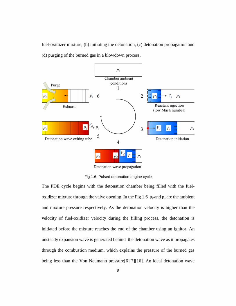
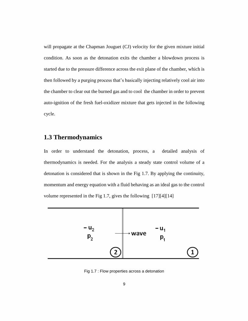
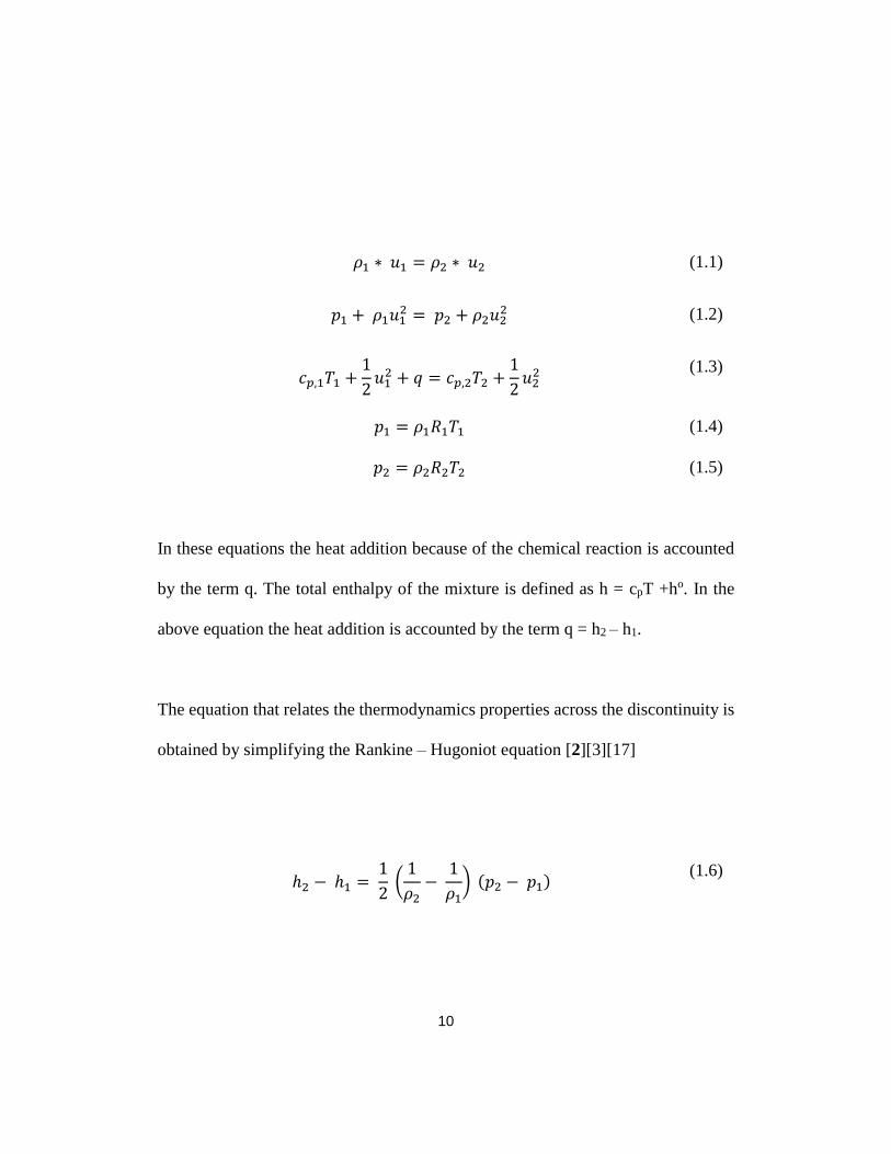
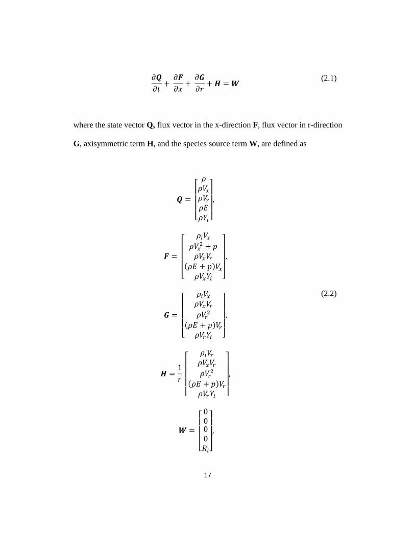
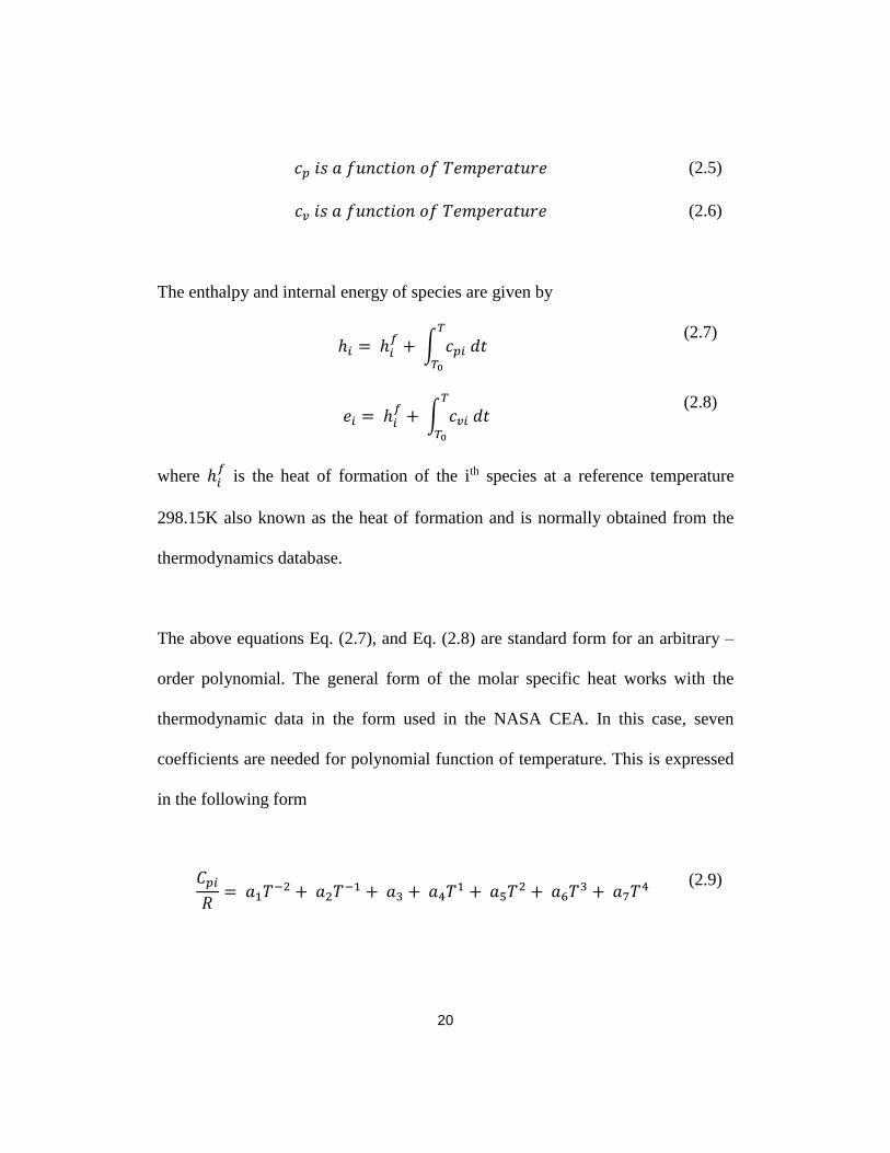
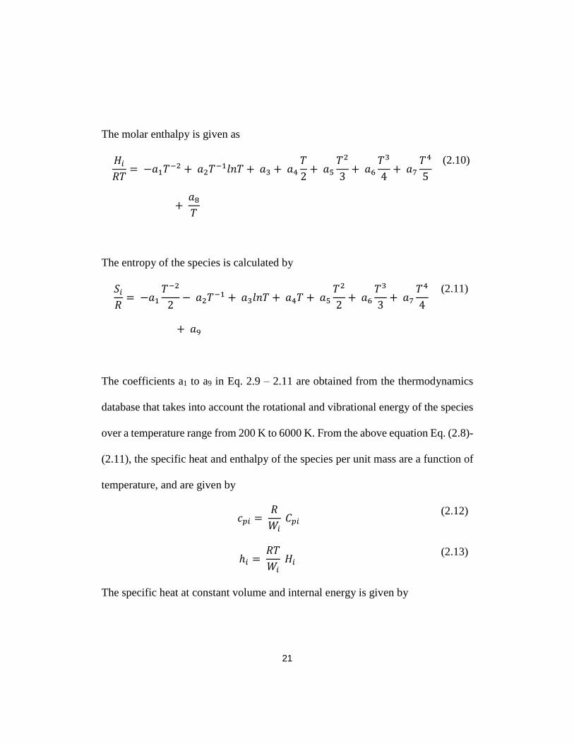