Numerical Simulation of Two-Dimensional Bubble Dynamics and ...

ARENBERG DOCTORAL SCHOOL

Faculty of Engineering Science

Numerical Simulation ofTwo-Dimensional BubbleDynamics and Evaporation

Xue Wang

Dissertation presented in partial

fulfillment of the requirements for the

degree of Doctor in Engineering

Science

May 2015

Supervisors:

Prof. Bart Blanpain

Prof. Jan Degrève

Numerical Simulation of Two-Dimensional Bubble

Dynamics and Evaporation

Xue WANG

Examination committee:Prof. Willy Sansen, chairProf. Bart Blanpain, supervisorProf. Jan Degrève, supervisorProf. Patrick WollantsProf. Frederik VerhaegheProf. Véronique Roig

(IMFT, Toulouse, France)Prof. Geraldine Heynderickx

(Ghent University, Belgium)

Dissertation presented in partialfulfillment of the requirements forthe degree of Doctorin Engineering Science

May 2015

© 2015 KU Leuven – Faculty of Engineering ScienceUitgegeven in eigen beheer, Xue Wang, Kasteelpark Arenberg 44 bus 2450, B-3001 Heverlee (Belgium)

Alle rechten voorbehouden. Niets uit deze uitgave mag worden vermenigvuldigd en/of openbaar gemaakt wordendoor middel van druk, fotokopie, microfilm, elektronisch of op welke andere wijze ook zonder voorafgaandeschriftelijke toestemming van de uitgever.

All rights reserved. No part of the publication may be reproduced in any form by print, photoprint, microfilm,electronic or any other means without written permission from the publisher.

Acknowledgments

“It is the time you have wasted for your rose that makes your rose so important.”– Antoine de Saint-Exupéry, The Little Prince

For me, pursuing a PhD is like planting a rose. It started with some budsof ideas, followed by sharp thorns, and finally ended with beautiful blossoms.In this marvelous adventure, many colleagues and friends encouraged me toconquer the thorns and gave me a hand to fertilize the soil. You all deserve agiant thank you!

Thank you, Prof. Bart Blanpain. I am proud of being your student. Back inOctober 2010, I wrote you an email that “I will come” and suddenly appearedin front of you. Now all of a sudden, it is time to leave. At this special moment,I would like to thank you for teaching me to write, to communicate, to playBoerengolf and to peel the potatos; thank you for teaching me to fish, insteadof giving me fish, even though you were deeply worried whether I would catchone; thank you for your patience and thank you for providing me a free andrelaxed environment. In China we have an old saying: "a teacher for a day is afather for a lifetime". All the things that you taught me can influence the restof my life.

Thank you, Prof. Jan Degrève, for being my promoter. Thank you for yourgenerous help when I am down; thank you for correcting my writing wordby word; thank you for teaching me to defend myself and thank you for yourcongratulations on my every tiny improvement. We can slove anything evenwithout MAOTAI.

Thank you, Prof. Frederik Verhaeghe. Without the interesting project that youwrote, I could not have the opportunity to come here. Thank you for beingour research line leader and for organizing a lot of valuable discussions. Thankyou, Prof. Patrick Wollants, for assessing my current work in all these yearsand for your advice and suggestions on the thesis. I also would like to thankProf. Geraldine Heynderickx and Prof. Véronique Roig. It is my great honor to

i

ii ACKNOWLEDGMENTS

have you in my jury. Thanks to both of you for reading my thesis very carefullyand for travelling twice to leuven to discuss in details. Thank you, Prof. WillySansen for taking your time and energy to chair my defences. Thanks to all ofyou for your unique contributions!

Thank you, Muxing. I will never forget the first two calls from you when I wasstill in China. Thank you for your encouragement and support. Sometimes itwas just a word or a look, but I can read it. Thank you, Prof. Jan Baeyens, forsharing life experience and delicious fish meal with me, also for your kindnessto my family.

Thank you, all the HiTemp group members (Pyro and Sremac). Time is magic.In the past few years, together, we shared the joy of HiTempers’ marriage (Bart,S & Y, Thomas, Huai, Huayue, Lichun, Bin. . . ), and witnessed the birth ofHiTemp babies (Hendrik, Zhaoqing, Ellie & Tiebe, Sofia, Eric, Pengpeng, Jade& Ruben, Lilly, Maria, Nicola. . . ). We have many wonderful academic activities,but also enjoy a lot of games (bowling, hiking, werewolves, cooking, drawing. . . ).Here, I would like to express my special thanks to some colleagues that relatedto my work. Thank you, Bart. You showed me the talent of a PhD and pavedthe way for my work. Thank you, Lesley, for the conference in Trondheim andthe Dutch abstract from Australia. Thank you, Chunwei, for the workshopin Dresden. Thank you, Vishal, Zhi and Bin, for your great ideas, inspiringdiscussions and selfless help. Thank you, Pengcheng, for your assistance inexperiments, for reading my manuscripts many times, and for pushing me all thetime. Thank you, my officemates Xiaoling, Prof. Nele Moelans, Philip, Qinggeand Prof. Raf Schouwenaars, for your company and support. Thank you, all thecolleagues in MTM, especially the kind help from Dirk, Mia, Mieke, Huberte,Jennifer, Paul, Rudy, Olivier, Pieter, Louis, Danny, Britt, Joop, Gert and Joris.I wish to acknowledge the financial support from Research Foundation Flanders(FWO) under Grant No.0433.10N.

Thank you, Prof. Marie-Françoise Reyniers, for arranging the visit to yourgroup. The stay in LCT, UGent is enjoyable and fruitful. Thank you, Amit.Your deep thinking and solid knowledge can always broaden my horizons andimprove my understandings. Thanks to all the colleagues there for treating mefriendly. The happy hours and the birthday chocolates are memorable.

Also, there are many friends in Leuven I would like to thank. Thank you,Pengcheng, for showing me the fabulous sports centre when I was staying athome all day long. Thank you for being my coach, sports partner and mentorat the same time. Thank you, Xiebin, for guiding me all the time and spendinga lot of time revising my thesis. Thank you, Ling, for bringing me to manybeautiful places. Thank you, Xuan, for the best organizations of our trip. Thankyou, Xiaoling & Zhi, for taking care of me for a very long time; thank you, Hao

ACKNOWLEDGMENTS iii

& Bin, for providing me help whenever I need it; thank you, Wenxu & Xuan forletting me not alone during the Chinese new year; thank you, Yichen & Jian, forshowing our family the beauty of Germany; thank you, Xiaodong, Minxian &Huayue, Chunwei and Chen for the wonderful get-together; thank you, Liugang& Yanyan, for the Beijing Roast Duck from Brussels; thank you, Lichun &Jiemei, for the home-made food; Thank you, Fei & Gong, Yuanyuan, Jingjing &Ji, Huili, Yujie, Shuigen, Qingge, Luman, Zhuangzhuang for making my stay inMTM colorful. Thank you, Yanyan, Yu, Lei, Ling, Zhe, Yejun, Tiannan, Hongand Jun for a lot of fun together. Specially, thank you, Yanyan, for providingme experimental materials and temporary accommodation.

Finally, I thank my family for their endless support. Thank you, my husband,for your broad shoulders and unconditional love. Thank you, my parents, forraising me up. Thank you, my sister and brother, for sharing the joys andsorrows. Thank you, my parents-in-law, for treating me as your own daughterand for putting all your efforts to my daughter. Thank you, my lovely daughter,for being happy every day. Mum is coming home and this thesis is for you!

Abstract

Gas bubble-melt interaction plays an important role in non-ferrous and ferrousmetallurgical processes. During these processes, gas is injected into a metal bathfor stirring or to add reactants at high temperature. The study of characteristicsof liquid metal dynamics remains a challenge due to the limitations of currentobservation methods. The situation is further complicated as mass and heattransfer occur during the interaction. On the other hand, water has a similarkinematic viscosity as liquid metal, and therefore can be used to simplifythe experimental situation for observations. Combined with proper numericalsimulations, the gas bubble-water interaction can be extended to gas bubble-meltinteraction, and can provide a partial insight in interactions at high temperature.In the present work, the gas bubble-liquid interaction is investigated based on amesoscopic two-dimensional multiphase CFD (Computational Fluid Dynamics)model. The main research work is divided into two parts: (1) 2D numericalsimulations of the quasi-two-dimensional inert bubble dynamics in liquid waterand experimental validation. (2) 2D numerical simulations of bubble dynamicsand evaporation in hot water.

In the first part, the buoyancy-driven single bubble behavior in a vertical Hele-Shaw cell was studied experimentally and numerically. The bubble behavior wassimulated by taking a two-dimensional volume of fluid (VOF) method coupledwith a continuum surface force (CSF) model and a wall friction model. Byadjusting the viscous resistance values, the bubble dynamics in different gapthicknesses were simulated. The first simulations were carried out in a narrowcell (cell width W = 5 cm) with two gap thicknesses (h = 0.5 mm and 1.0 mm).For the main bubble flow properties including shape, path, terminal velocity,horizontal vibration and shape oscillation, a good agreement is obtained betweenexperiment and simulation. The simulation confirms that the thin liquid filmspresent between gas bubbles and the cell walls have a limited effect on thebubble dynamics.

The simulations were then expanded into four gap thicknesses and the effects

v

vi ABSTRACT

of gap thickness on the bubble dynamics were discussed. It was found in bothexperiments and simulation that with an increased spacing between the cellwalls, the bubble shape changes from oblate ellipsoid and spherical-cap to morecomplicated shapes while the bubble path changes from only rectilinear to acombination of oscillating and rectilinear; the bubble drag coefficient decreasesand this results in a higher bubble velocity caused by a lower pressure exerted onthe bubble; the wake boundary and wake length evolve gradually accompaniedby vortex formation and shedding. Finally, the simulations were extended toa wide Hele-Shaw cell (W = 40 cm). The simulated bubble-induced liquidvelocity and the released vorticity were compared with Roig et al.’s experimentalmeasurements.

In the second part, the liquid water evaporating into the gas bubble wassimulated by incorporating interfacial mass transfer at the interface grid cellsbetween the liquid and gas bubble. The coupling between momentum andmass transfer was incorporated using a user-defined function (UDF). Thelocal evaporation rate was derived from the Hertz-Knudsen equation. Themeasurements of Pauken for water evaporation rate in a moving air streamwere used to mimic the interfacial evaporation at the bubble interface. The gridindependence of the interfacial mass transfer flux was proven. The evolution ofmass transfer rate and mass concentration in the bubble can be captured, aswell as the interaction of the mass transfer and hydrodynamic properties.

Beknopte samenvatting

De interactie tussen een gasbel en de vloeistof speelt een belangrijke rol innon-ferro en ferro-metallurgische processen. In deze processen wordt een gasgeïnjecteerd in het metaalbad voor het mengen of voor de toevoeging vanreactanten bij hoge temperatuur. Enerzijds blijft studie naar de karakteristiekekenmerken van metaalhydrodynamica een uitdaging, vanwege de beperkingenvan de huidige observatietechnieken. Het gelijktijdig optreden van massa-en warmtetransport met de gas-vloeistof interacties maakt de situatie nogingewikkelder. Anderzijds heeft water een gelijkaardige kinematische viscositeitals vloeibaar metaal, waardoor het als substituut kan dienen en hiermee deobservaties aan de hand van experimenten vereenvoudigt. In combinatie metgepaste numerieke simulaties kan het een gedeeltelijk inzicht bieden in deinteracties op hoge temperatuur. In het huidig werk wordt de gasbel-vloeistofinteractie onderzocht aan de hand van een mesoscopisch, twee-dimensioneel,multifase CFD (computationele vloeistofdynamica) model. Het onderzoek isopgedeeld in twee delen: (1) Een 2D numerieke simulatie en experimentelevalidering van de quasi-twee-dimensionele interactie tussen een inerte gasbel enwater. (2) Een 2D numerieke simulatie van de beldynamica en verdamping inwarm water.

In het eerste deel wordt eerst het gedrag van één enkele opwaartse gasbelexperimenteel en numerisch bestudeerd aan de hand van een verticale Hele-Shawcel. Het belgedrag werd gesimuleerd gebruikmakend van een twee-dimensioneleVolume-of-Fluid (VOF) methode, gekoppeld met het Continuum Surface Force(CSF) model en een model voor de wrijving met de wand. Door aanpassing vande viskeuze weerstandswaarden kan de beldynamica voor verschillende diktesvan de opening bestudeerd worden. De initiële simulaties werden uitgevoerdvoor een smalle cel (celbreedte W = 5 cm) met twee diktes (h = 0.5 en 1.0mm). Een goede overeenkomst tussen experiment en simulaties werd bekomenvoor de algemene beldynamica eigenschappen, zoals vorm, traject, eindsnelheid,horizontale trillingen en vormveranderingen. De simulaties bevestigen dat dedunne vloeistoffilm tussen de gasbel en de wand slechts een beperkte invloed

vii

viii BEKNOPTE SAMENVATTING

heeft op de beldynamica.

Vervolgens werden de simulaties uitgebreid naar vier diktes en werd het effectvan de dikte op de beldynamica bestudeerd. In zowel de experimenten alsde simulaties werd bevonden dat, met een toenemende dikte, de vorm vande bel overgaat van een afgeplatte ellipsoïde en een bolkap gasbel naar meeringewikkelde vormen, terwijl het beltraject overgaat van rechtlijnig naar eencombinatie van oscillerend en rechtlijnig; de belwrijvingscoëfficient neemt afen dit leidt tot een hogere snelheid vanwege een lagere druk uitgeoefend opde bel; de grens en lengte van het kielzog neemt geleidelijk aan toe en wordtvergezeld van vorming en afstoten van vortices. Als laatste werden de simulatiesverder uitgebreid naar een brede Hele-Shaw cel (W = 40 cm). De berekendevloeistofsnelheid, opgewekt door de gasbel, en de vrijgekomen vorticiteit werdenvergeleken met de experimenteel opgemeten waarden van Roig et al.

In het tweede deel wordt een simulatie uitgevoerd van de verdamping van waternaar de gasbel door het in rekening brengen van het grensvlakmassatransportin de roostercellen met een grensvlak. De koppeling tussen de momentum-en massaoverdracht werd ingebouwd aan de hand van een zelfgeschrevensubroutine (User-Defined Function; UDF). De lokale verdampingssnelheid werdbekomen door middel van de Hertz-Knudsen vergelijking. De verdampingaan het grensvlak werd nagebootst aan de hand van verdampingssnelhedenin een luchtstroom, verkregen uit de experimenten van Pauken. De flux vanhet grensvlakmassatransport werd getest op roosteronafhankelijkheid. Het ismogelijk zowel de evolutie van massaoverdrachtsnelheid, de massaconcentratiein de gasbel, als de interactie tussen de massaoverdracht en de hydrodynamischeeigenschappen vast te leggen.

Nomenclature

α Viscous resistance [m2]γ Volume fraction

δfilm Film thickness [m]

η Evaporation coefficientκ Curvature [m−1]

Λ Thermal conductivity [W·m−1·K−1]µ Dynamic viscosity [Pa·s]ν Kinematic viscosity [m2·s−1]ρ Average density [kg·m−3]σ Surface tension [N·m−1]τ Dimensionless timeϕ Velocity constantχ Mole fractionω Mass fraction

Ω Vorticity [s−1]

A Interface area [m2]

Ar Archimedes number

Bo Bond numberc Evaporation parameter [s·m−1]cA Concentration [mol·m−3]cp Heat capacity [J·kg−1·K−1]

Ca Capillary number

CD Drag coefficient

d Bubble diameter [m]

D Diffusion coefficient [m2·s−1]

E Energy [J·kg−1]

Eo Eötvös number

ix

x NOMENCLATURE

Es Energy source term [J·m−3·s−1]

e Aspect ratio

f Frequency [s−1]

f1 Horizontal velocity frequency [s−1]

f2 Perimeter oscillation frequency [s−1]

F Force source term [N·m−3]

Fσ Surface tension source term [N·m−3]

Fw In-gap wall friction source term [N·m−3]

g Gasg Gravity acceleration [m·s−2]

h Gap thickness [m]

H Heat capacity [J·kg−1]

∆Hvap Latent heat of vaporization [J·kg−1]

i Phase index

j Species index

J Diffusion flux [kg·m−2·s−1]

J ′ Evaporation flux [kg·m−2·s−1]

K Mass transfer coefficient [m·s−1]

l Liquid

L Perimeter [m]

Lwake Wake length [m]

M Molar mass [kg·mol−1]

m Mass transfer rate [kg·m−3·s−1]nA Mass transfer rate [mol·s−1]p Pressure [Pa]p0 Pressure at bubble nose [Pa]

Pe Peclet numberpmod Modified pressure [Pa]psat Saturated vapor pressure [Pa]r Radius [m]rc Radius of curvature at the front stagnation

point[m]

R Universal gas constant [J·mol−1·K−1]

Re Reynolds number

Re(h/d)2 Gap Reynolds number

S Area [m2]

Sc Schmidt number

Sh Sherwood number

NOMENCLATURE xi

t Physical time [s]

T Temperature [C] or [K]

Tref Reference temperature [C] or [K]

u Fluid velocity vector [m·s−1]uaxis Vertical velocity when y = 0 [m·s−1]ub Bubble terminal velocity [m·s−1]ux Horizontal velocity [m·s−1]ux0 Horizontal velocity amplitude [m·s−1]uy Vertical velocity [m·s−1]

V Volume [m3]

Vcell Volume of the grid cell [m3]

W Cell width [m]x Horizontal position [m]y Vertical position [m]

2D Two-dimensional

3D Three-dimensional

CFD Computational fluid dynamics

CSF Continuum surface force

PLIC Piecewise linear interface construction

PLIF Planar laser-induced fluorescence

PIV Particle imaging velocimetry

SIMPLE Semi-Implicit-Method for Pressure LinkedEquations

SLIC Simple linear interface construction

UDF User-defined function

VOF Volume of fluid

Contents

Abstract v

Nomenclature ix

Contents xiii

1 General Introduction 1

1.1 Introduction . . . . . . . . . . . . . . . . . . . . . . . . . . . . . 2

1.1.1 Gas injection in pyrometallurgical processes . . . . . . . 2

1.1.2 Silicon tetrachloride injection in liquid zinc . . . . . . . 3

1.2 Objectives of the thesis . . . . . . . . . . . . . . . . . . . . . . 4

1.3 Outline of the thesis . . . . . . . . . . . . . . . . . . . . . . . . 5

2 Literature Review 7

2.1 Experimental work . . . . . . . . . . . . . . . . . . . . . . . . . 8

2.1.1 Bubble dynamics and mass transfer in liquid metal . . . 8

2.1.2 Bubble dynamics and mass transfer in liquid water . . . 12

2.1.3 Bubble dynamics in a Hele-Shaw cell . . . . . . . . . . . 22

2.2 Numerical simulation . . . . . . . . . . . . . . . . . . . . . . . . 23

2.2.1 Simulation methods . . . . . . . . . . . . . . . . . . . . 25

xiii

xiv CONTENTS

2.2.2 Bubble dynamics and mass transfer in simulation . . . . 29

2.3 Conclusions . . . . . . . . . . . . . . . . . . . . . . . . . . . . . 33

3 2D Bubble Dynamics 35

3.1 Introduction . . . . . . . . . . . . . . . . . . . . . . . . . . . . . 36

3.2 Experimental setup . . . . . . . . . . . . . . . . . . . . . . . . . 37


3.3.1 Governing equations . . . . . . . . . . . . . . . . . . . . 40

3.3.2 Simulation strategies . . . . . . . . . . . . . . . . . . . . 42

3.4 Results and discussion . . . . . . . . . . . . . . . . . . . . . . . 43

3.4.1 Results for gap thickness h = 0.5 mm . . . . . . . . . . 43

3.4.2 Results for gap thickness h = 1.0 mm . . . . . . . . . . 49

3.4.3 Discussion . . . . . . . . . . . . . . . . . . . . . . . . . . 56

3.5 Conclusion . . . . . . . . . . . . . . . . . . . . . . . . . . . . . 60

4 Effect of Gap Thickness 61

4.1 Introduction . . . . . . . . . . . . . . . . . . . . . . . . . . . . . 62


4.3 Experimental validation . . . . . . . . . . . . . . . . . . . . . . 64


4.4.1 Bubble shape and path . . . . . . . . . . . . . . . . . . 65

4.4.2 Bubble Reynolds number and drag coefficient . . . . . . 67

4.4.3 Pressure field and velocity field . . . . . . . . . . . . . . 69

4.5 Conclusions . . . . . . . . . . . . . . . . . . . . . . . . . . . . . 74

4.6 Appendix . . . . . . . . . . . . . . . . . . . . . . . . . . . . . . 75

5 Drag Coefficient and Bubble Wake 77

5.1 Introduction . . . . . . . . . . . . . . . . . . . . . . . . . . . . . 78

CONTENTS xv


5.3 Results and discussion . . . . . . . . . . . . . . . . . . . . . . . . 81

5.3.1 Bubble shape and path . . . . . . . . . . . . . . . . . . . 81

5.3.2 Bubble velocity coefficient and drag coefficient . . . . . 82

5.3.3 Bubble wake . . . . . . . . . . . . . . . . . . . . . . . . 83

5.4 Conclusions . . . . . . . . . . . . . . . . . . . . . . . . . . . . . 87

6 2D Bubble Dynamics and Evaporation Simulation 89

6.1 Introduction . . . . . . . . . . . . . . . . . . . . . . . . . . . . . 90

6.2 Numerical simulation . . . . . . . . . . . . . . . . . . . . . . . . . 91

6.2.1 Governing equations . . . . . . . . . . . . . . . . . . . . 92

6.2.2 Simulation strategies . . . . . . . . . . . . . . . . . . . . 95


6.3.1 Effect of evaporation parameter . . . . . . . . . . . . . 96

6.3.2 Concentration and temperature distributions . . . . . . 97

6.3.3 Effect of shape oscillation . . . . . . . . . . . . . . . . . 100

6.3.4 Effect of bubble size . . . . . . . . . . . . . . . . . . . . 102

6.3.5 Effect of temperature . . . . . . . . . . . . . . . . . . . 104

6.4 Conclusions . . . . . . . . . . . . . . . . . . . . . . . . . . . . . 105

7 Conclusions and Outlook 107

7.1 General conclusions . . . . . . . . . . . . . . . . . . . . . . . . . 108

7.2 Future work . . . . . . . . . . . . . . . . . . . . . . . . . . . . . 110

A Physical properties of SiCl4-Zn system and N2-H20 system 113

A.1 SiCl4-Zn system . . . . . . . . . . . . . . . . . . . . . . . . . . 113

A.2 N2-H2O system . . . . . . . . . . . . . . . . . . . . . . . . . . . 114

B The Illustration of Interface mass transfer model 117

xvi CONTENTS

Bibliography 121

Curriculum Vitae 135

List of Publications 137

Chapter 1

General Introduction

In this chapter, a brief introduction to the research topics, outline of the projectand the structure of the thesis is presented.

1

2 GENERAL INTRODUCTION

1.1 Introduction

1.1.1 Gas injection in pyrometallurgical processes

The injection of gas into liquid metals is widely used in pyrometallurgicalprocesses such as nickel and copper converting, steelmaking, and chloride fluxingof aluminum (Figure 1.1). Diverse needs can be achieved by these gas injectionsteps, for example, fluxing a chlorine and nitrogen gas mixture through the liquidaluminum for degassing, removal of impurities like magnesium, nonmetallicinclusions and alkali metals [1]. In steelmaking, gas injection is applied toenhance reaction rates, eliminate thermal and compositional gradients and toremove nonmetallic inclusions [2].

Figure 1.1: Typical gas injection systems in pyrometallurgy. (a) copperconverting1; (b) chloride fluxing of aluminum2.

Gas injection may be achieved with different types of injection devices suchas tuyeres, porous plugs, or a lance, and the gas may be blown from the top,side or bottom of the furnace. Upon injection, buoyancy-driven gas bubbles aredispersed within a continuous liquid phase. The high surface area-to-volumeratio of the bubbles greatly increases the gas/liquid contact area and providesexcellent mass and heat transfer characteristics at the gas/liquid interface.Meanwhile, the bubble column has the advantages of easy construction, lowcost and simple operation [3].

1http://www.dundeeprecious.com/files/images/projects/pierce_smith_furnace.jpg2http://www.autumnfjeld.com/autumnfjeld/wordpress/wp-autfiles/old_silly_site/

files/AutumnResearchMar16.pdf

INTRODUCTION 3

Despite the widespread industrial applications, the detailed understandingof the fluid mechanics prevailing in bubble column reactors is unfortunatelystill lacking [4]. The performance of the bubble column reactor relies on thecombined outcome of multiphase fluid dynamics, interfacial mass transfer andchemical reactions (when the gas is reactive). The bubble column reactors covera wide range of spatial scales which span about 7 orders of magnitude (Figure1.2). It would be a difficult task to understand the details at all scales withinand surrounding the bubble. The current work focuses on the phenomena onthe meso-scale due to the following reasons [5]: (1) the meso-scale is the mostinformative scale to understand the whole range of scales, and it is the bridgebetween the micro-scale nature and the macro-scale appearance; (2) in-depthunderstanding of the meso-scale structure is critical to scale-up of real sizereactors, and (3) the meso-scale structure is still a common challenge, its effectson the flow, heat/mass transfer have not been understood well and literatureshows striking differences.

Figure 1.2: Multi-level modelling of bubble column reactors [6, 7].

1.1.2 Silicon tetrachloride injection in liquid zinc

Silicon tetrachloride gas injection in liquid zinc is an ideal case study of gasinjection into melts. The characteristics of this process are that SiCl4 gas isinjected into liquid zinc at operating temperatures above the boiling pointof ZnCl2 (732C) but below the boiling point of liquid zinc (906C), and Siparticles are formed due to reductive reactions (see Appendix A for the physicalproperties of SiCl4-Zn system). Ideally, a temperature between 850-880C ispreferable to keep the zinc vapor pressure high. The phenomena accompaniedwith SiCl4 bubble rise are illustrated in Figure 1.3. During the bubble rise,the reduction can take place at the gas-liquid interface and in the bulk of thebubble due to the evaporation of liquid zinc into the bubble. Correspondingly,


solid silicon is generated in the bulk gas phase or at the bubble interface. It candissolve in the liquid zinc and float at the top of the liquid melt due to densitydifference. Therefore, a complete description of the system should include masstransfer of evaporation, gas-gas reaction, gas-liquid reaction and dissolution,also their interaction with bubble dynamics and the corresponding heat transfer.

Figure 1.3: Illustration of SiCl4(g)-Zn(l) system at micro- and meso-scales.

Even at the meso-scale, it is impossible to study all these phenomena in onemodel. Further simplification of the situation is necessary. From literature, itwas found that the reaction mostly proceeds under the gaseous state of SiCl4and Zn [8], which means the gas-liquid reaction can be reasonably neglected.Meanwhile, the bubble lifetime is measured in seconds, which is very short. Itis very difficult to track the Si particle on this small time scale. The Si can existin the gas phase due to formation, dissolve in the liquid phase, or remain in thesuspension as aggregate. Its existence changes continuously during the wholeinjection process which lasts for hours. Therefore, the focus of the present studyis on the bubble dynamics and mass transfer due to evaporation at meso-scale.

1.2 Objectives of the thesis

The main objective of the present study is to develop a numerical model topredict qualitatively and quantitatively the bubble dynamics of a gas bubbleand the associated liquid evaporation into the gas bubble. The choice for anumerical simulation study was made based on the fact that the experimentalmeasurement of detailed bubble flow properties is difficult due to the opacity ofliquid metal and high temperature characteristics. In this study, the simulation

OUTLINE OF THE THESIS 5

is not directly focused on the gas bubble in liquid metal, instead, liquid waterwill be used due to its similar hydrodynamic properties, its ease of handling andits availability of the quantified liquid characteristics. Therefore, the followingobjectives will be pursued:

(1) To simulate numerically the two-dimensional bubble dynamics, to discoverthe characteristics of the bubble properties such as bubble shape and bubbleterminal velocity, extracting the liquid flow properties, such as liquid velocityand liquid vorticity.

(2) To validate the simulated bubble dynamics quantitatively with our ownexperiments and available literature.

(3) To couple the evaporation-induced micro-scale interface mass transfer withphase change into the meso-scale bubble dynamics.

(4) To investigate the parameter effects on the liquid evaporation-inducedbubble growth numerically, also the interplay of bubble dynamics and bubbleevaporation on the bubble behavior.

1.3 Outline of the thesis

Two numerical models were developed, the first is the two-dimensional bubbledynamics model, and the second is the two-dimensional bubble dynamics andevaporation model. Chapters 3–5 are on the description of the first model andexperimental validation. Chapter 6 is devoted to the second model.

Chapter 2 involves a review of some important aspects of bubble dynamicsand bubble mass transfer related to this study. A brief review on the bubbledynamics and mass transfer in liquid metal and in liquid water in both three-and two-dimensions is provided. Both experimental observations and numericalsimulations are presented.

Chapter 3 is concerned with the model development and the numerical solutionmethods. A detailed description of the governing equations is presented andthe numerical schemes employed to solve them are introduced. As a test, themodel is developed to simulate the bubble dynamics of a nitrogen gas bubble (26 d 6 25 mm, d bubble diameter) in liquid water in a narrow cell (Figure 2.8,cell width W = 5 cm) at room temperature. The averaged properties of bubbleshape, bubble path, bubble terminal velocity, as well as the secondary motionof shape oscillation and horizontal vibration, are simulated and compared withour own experimental measurements.


Chapter 4 discusses the effects of gap thickness on the bubble dynamics andpresents the bubble flow properties as a function of the gap thickness. Meanwhile,the coupling of pressure distribution and velocity distribution in the wake isdiscussed based on the simulated results.

Chapter 5 further extends the studies to a wide cell with an aim to provide aquantitative simulation of the bubble wake. The general velocity coefficient anddependency on gap thickness are found. The simulation shows a quantitativeagreement with experiments performed by Roig et al. [9].

Chapter 6 presents a numerical study of bubble dynamics and evaporation.In this study, numerical investigations are conducted into the bubble growthof a two-dimensional nitrogen bubble in water at higher temperatures whichis below the liquid boiling point. The model is based on the coupling of theinterface mass transfer and bubble dynamics. The effects of bubble size, shapeoscillation, temperature and evaporation coefficient on mass transfer rate atgas/liquid interface are discovered.

Chapter 7 summarizes the major conclusions and discusses some suggestionsand recommendations for future work.

Chapter 2

Literature Review

This chapter gives a comprehensive literature review on bubble dynamics andmass transfer in liquid metal and water, in both two- and three-dimensions.The numerical simulation methods available for bubble dynamics and masstransfer are also discussed, together with their applications.

7

8 LITERATURE REVIEW

2.1 Experimental work

2.1.1 Bubble dynamics and mass transfer in liquid metal

Bubble dynamics

In the study of mesoscopic bubble dynamics, the overall bubble flow propertiessuch as bubble shape, bubble trajectory and bubble terminal velocity areimportant for stirring and mass transfer. Meanwhile, the details of the gascirculation inside the bubble and the bubble-induced liquid flow in the bubblewake are indispensable for a full understanding of the complex two-phase flowand mass transfer. However, in the studies of single bubble behaviour in liquidmetal, progress is quite slow due to the difficulty in conducting experiments athigh temperatures and due to the opacity of the melt.

Figure 2.1: Spherical-cap bubbles in mercury and water. (a) A two-dimensionalargon bubble (base 8 cm) rising in mercury [10]. (b) A nitrogen bubble (base7.3 cm) rising in a column of water [11].

In the 1960s, Davenport and his colleagues carried out experiments on largespherical-cap bubbles rising in mercury and silver in both three-dimensionalcolumns [10] and semi-two-dimensional columns [12]. The bubble shape and risevelocity were detected. In the three-dimensional experiments, the bubble shapewas measured by means of electrical probes. For a direct visualization of thebubble interface, semi-two-dimensional experiments were carried out. Also in1968, Schwerdtfeger measured the argon bubble velocities in a three-dimensionalliquid mercury column with an ultrasonic pulse-echo instrument [13]. Thoughthese experiments are nearly 50 years old and the measurements are rough, they

EXPERIMENTAL WORK 9

obtained very important information on the bubble shape and bubble terminalvelocity in liquid metal.

The shapes of spherical-cap bubbles observed by Paneni & Davenport [12] aresimilar in thin sheets of water and mercury (the sheets are wide enough that thebubbles in both cases do not touch the walls), except that the higher surfacetension of mercury increases the radius of curvature at the bubble’s trailing edge(Figure 2.1). They also found that shapes are similar in two-dimensional andthree-dimensional systems. For the bubble rise velocity, Davenport et at. [10]found that the velocities of bubbles rising in mercury and in water are similar( bubble diameter 10 < d < 48 mm). The measured velocity is smaller thanthe theoretical expression of ub = 0.67(grc)0.5 or ub = 1.02(gr)0.5 (EQ. (8.3.6)in Figure 2.2a. ub bubble terminal velocity, g gravity acceleration, rc radius ofcurvature, and r bubble radius). The constricting effects of the walls in theexperiments attribute to the reduced terminal velocity. In Schwerdtfeger’s study,smaller bubble sizes were studied (2 < d < 15 mm). The terminal velocities inliquid mercury and in liquid water still show similarities (Figure 2.2b) [12].

Figure 2.2: Rising velocities of bubbles in water and in mercury. (a) Velocitiesof spherical-cap air bubbles rising in mercury and in water [10]. (b) Velocitiesof small argon bubbles in mercury and distilled water at room temperature [13].

The recent study on bubble dynamics in liquid metal can be divided intotwo categories, one about liquid velocity measurements, the other related tovisualization of the bubble contour:

(1) Liquid velocity measurements

The techniques of local and instantaneous measurements in liquid metals areknown to be much more difficult than in classical transparent fluids like water andair [14]. The conventional measuring techniques used for ordinary flows include

10 LITERATURE REVIEW

(a) flow visualization, (b) measurement of velocities with differential pressure, (c)electromagnetic velocity measurement, (d) hot wire and hot film anemometry,(e) laser-Doppler velocimetry and (f) ultrasound Doppler velocimetry [15]. Mostof the methods fail in liquid metal flows, or their applicability is stronglylimited [14]. The application of ultrasound Doppler velocimetry to liquidmetal flows has been found promising. Reliable results were obtained in liquidmercury, gallium and eutectic alloy GaInSn at low temperatures. The rangeof applicability has been extended to flows of liquid sodium(150C), to PbBibubbly flow (180–300C) and CuSn flow at temperatures of about 620C [16].However, due to the lacking of bubble shape and path, reconstruction of bubblewake structure is difficult.

(2) Visualization of bubble contour

Table 2.1: Comparison of bubble visualization techniques in liquid metal [17–19].

Category Methods Advantage Disadvantage

X-ray photography Fast datacollection

Expensive to operate

DirectVisualization Neutron radiography Graphical Strong attenuation

Non-contact

Thermal sensor Simple design Slow response

Indirect probemeasurement

Electric resistivity sensor Durable Low accuracy

Capacitance probe Contacting liquid

The measurement techniques that can be used to visualize the bubble in liquidmetal in three-dimensions are summarized in Table 2.1. These techniques fallunder two general categories, namely direct visualization techniques and indirectprobe measurements [17]. The optical approach is widely used in water-basedsystems, however, optical techniques cannot work in liquid metals because visiblelight cannot be transmitted in liquid metals. Therefore, radiographic imagingsuch as X-rays and neutron beams is needed. In the second category, the propertydifferences between the gas phase and the liquid phase are exploited. Theseinclude electrical properties, thermal conductivity and mechanical properties.Among all these techniques, high energy X-rays and electroresistivity probeattract more attention. However, these two methods are not able to provideaccurate information on the bubble shape. The bubble contour obtained by theelectric probe is composed of a limited number of vertical cross sections, resultingin a low resolution and large error (Figure 2.3a). The image by radiography can

EXPERIMENTAL WORK 11

provide a better quality, however, the bubble shapes show a jagged interfacedue to image noise (Figure 2.3b). Another limitation for radiography is that thesize of the container is limited due to severe light attenuation. The thicknessof the tank used in [19] is 30 mm. None of these techniques are applicable tosmall bubbles since the dimensions become comparable to the resolutions.

Figure 2.3: Comparison of the images captured by different techniques. (a)Two successively rising bubbles with multineedle electroresustivity for Wood’smetal-He system [18]. The 3D experiment was carried out in a cylindricaltest vessel wih an inner diameter of 200 mm and a height of 300 mm. (b) Aspherical cap water vapor bubble in a liquid Pb-Bi alloy with high-frame-rateneutron radiography [19]. The 3D rectangular dimensions are 400 mm height,80 mm width and 30 mm thickness. (c) Air bubbles in mercury under semi-two-dimensional flow conditions, in a thin sheet of 800 mm high by 300 mmwide and 4.7 mm thick [12]. (d) Two nitrogen bubbles in liquid mercury (upperone) and in liquid zinc (lower one) in a Hele-Shaw cell with dimensions of 450mm height 50 mm width 1.0 mm thickness, and 490 mm height 95 mm width1.5 mm thickness, respectively [20].

To overcome the three-dimensional visualization difficulties and to provide highresolution of bubble contours, very recently in 2014, Klaasen et al. [20] tried toconfine the bubble in two-dimensions in a Hele-Shaw cell. The cell is composedof two parallel transparent walls separated by a small gap. The thickness of thegap is 1.0 or 1.5 mm, which is much smaller than that of Paneni and Davenport(1 cm) [12]. Together with a proper non-wetting transparent wall, the bubbles inliquid mercury (room temperature) and liquid zinc (700C) were visualized with


ease by a high-speed camera. Through the comparison of the bubble contoursobtained by the above mentioned experiments (Figure 2.3), it is apparent that,in the near future, the two-dimensional technique has the advantage of providingmore details on the bubble dynamics as well as on the mass transfer withoutthe difficulties present in the three-dimensional observations.

Mass transfer

The studies on bubble mass transfer in liquid metal are very few. For theliquid-side mass transfer coefficient, Davenport et al. measured the masstransfer coefficient of large spherical-cap bubbles in three dimensions by pressurechange [10]. The rates of absorption of oxygen by liquid mercury and moltensilver have been interpreted [10]. The measured overall mass transfer coefficientof oxygen into mercury Kl is 0.055 cm·s−1, into liquid silver is 0.036 ± 0.007cm·s−1 (1000C). Although the error for measurement in the liquid metal wasestimated to be ±30–40%, the detected liquid-side mass transfer coefficient issimilar to that of CO2-H2O system (The overall mass transfer coefficient ofabout 0.026 cm·s−1 was observed for CO2-H2O system at 15C). The masstransfer coefficient was estimated by Kl = 0.82r−0.25D0.5g0.25 (Kl liquid phasemass transfer coefficient, D diffusion coefficient). For gas-side mass transfer,the studies are only on the macro-scale mass transfer coefficient (KgA) whereinterface mass transfer area A is unknown [21,22].

In conclusion, a full understanding of mesoscopic bubble dynamics in three-dimensions is still lacking due to poor image resolution, while a two-dimensionalvisualization can provide more details. The available studies confirm that thebubble dynamics and mass transfer coefficient are similar in liquid metal and inliquid water due to similar mass and momentum transport properties. Therefore,it is possible to use a water model to simulate the liquid metal situation basedon the similarity criteria.

2.1.2 Bubble dynamics and mass transfer in liquid water

Unlike the slow progress of the bubble dynamics in liquid metal, numerousstudies of bubbles in liquid water have been carried out since the 1950s. Noattempt has been made to provide a complete list of the available experimentaltechniques and results in literature. The works by Davies & Taylor [23],Davenport [24], and Clift, Grace & Weber [25] provide a guide to the underlyingtheory of the fluid dynamics associated with bubbles moving in a liquid medium.The reviews can be found elsewhere [26, 27]. Here a short review on bubbledynamics and mass transfer is presented.


Dimensionless parameters

In general, a gas bubble rising in an infinite liquid medium is dependent on thephysical properties of the surrounding fluid. These properties include the densityof liquid phase ρl, the density of gas phase ρg, the viscosity of liquid phase µl,the viscosity of gas phase µg, the surface tension σ, equivalent diameter of thegas bubble d. The three-dimensional bubble diameter d is defined by:

d = 2

(

3V

4π

)1/3

(2.1)

where V is the bubble volume. The two-dimensional bubble diameter d isdefined by:

d = 2

(

S

π

)1/2

(2.2)

where S is the bubble area in the plane.

The consideration of gas phase density and viscosity is normally ignored dueto small values compared to that of the liquid phase. Besides these properties,the bubble terminal velocity ub is also an important parameter though it is notindependent.

The following dimensionless parameters are used to describe the bubbledynamics:

Reynolds number:

Re =inertial force

viscous force=

ρludd

µl(2.3)

Eötvös number:

Eo =buoyancy force

surface tension force=

ρlgd2

σ(2.4)

Weber number:

We =inertial force

surface tension force=

ρlu2

bd

σ(2.5)

Morton number:

Mo = EoWe2

Re4=

gµ4

l

ρlσ3(2.6)

Drag coefficient:

CD =We

Eo=

4gd

3u2

b

(2.7)


Similarly, for gas bubble mass transfer, except for the above mentioned physicalproperties, the diffusion coefficient D and mass transfer coefficient K are alsoimportant. The mass transfer coefficient K is defined as:

K =nA

A∆cA(2.8)

where nA is the mass transfer rate; A is the mass transfer area; ∆cA is thedriving force concentration difference.

The corresponding dimensionless numbers include:

Schmidt number:

Sc =viscous diffusion rate

mass diffusion rate=

µ

ρD(2.9)

Péclet number:

Pe =convective transport rate

diffusive transport rate= Re · Sc (2.10)

Sherwood number:

Sh =convective mass transfer coefficient

diffusive mass transfer coefficient=

Kd

D(2.11)

Bubble shape

The shape of a rising bubble is determined by the pressure distribution alongthe interface layer and the shape is therefore defined by the mutual interactionof surface tension, viscosity, buoyancy and inertial forces [27]. Clift et al. [25]provided a graphical correlation of the shapes of bubbles and drops in terms ofRe, Eo and Mo (Figure 2.4).

For a gas bubble in liquid water, the physical properties of density, kinematicviscosity and surface tension are constant, the bubble shape is therefore mainlydependent on the bubble size. The Morton number of water is 10−11, which isvery close to the liquid metal Morton range of 10−11.8-10−13.8 [20]. Therefore,the bubbles can be grouped in the following three categories [28]:

(a) Spherical bubbles

In this category, the bubble size is very small. They are approximated by aspherical shape in the low Reynolds number range, and they rise in a rectilinearpath.


Figure 2.4: Shape regimes for bubbles and drops in unhindered gravitationalmotion through liquids [25].

(b) Ellipsoidal bubbles

In this case, the bubble size is intermediate. They can take a variety of shapesexcept for an ellipsoidal shape. The bubbles show two types of secondary motionincluding shape oscillation and path instability.

(c) Spherical-cap bubbles

With a further incease of the bubble size, the shape of the bubbles in this rangecan be closely approximated with a spherical cap upper surface and a flat base.In the case of large bubbles, the effects of surface tension and viscosity arenegligible and the rise velocity is given by the equation of Davies and Taylor [23].

16

LIT

ER

AT

UR

ER

EV

IEW

Figure 2.5: Experimental studies of bubble shape, bubble path and bubble wake in the literature. For bubble shape,(a) d = 1.74 mm [29]; (b) d = 1.28 mm [30]; (c) d = 2.48 mm [31]; (d) d = 1.82 mm [30]; (e) d = 42 mm [25]. Forbubble path, (f) d = 1.37 mm [29]; (g) d = 1.52 mm [29]; (h) d = 2.24 mm [32]; (i) d = 2.48 mm [31]; (j) d = 1.58mm [33] (k) d = 2.02 mm [33]. (l) d lies in 0.66–0.93 mm in silicone oil [34]. (m) d lies in 4–8 mm, Re = 1500 [35], (n)d ≈ 45 mm [36], (o) d (unknown) [37].


The typical bubble shapes for the three types of bubbles are shown in Figure2.5a–e. Saffman [38] found that the transition size from the spherical bubbleto ellipsoidal bubble in tap water is d = 1.4 mm, while the value is d = 1.8mm in pure water by Duineveld [30] and d = 1.7 mm in pure water by Wu &Gharib [29]. The differences in the above studies demonstrated that the onset ofthe shape change is very complicated and dependent on the physical propertiesand contamination.

Terminal velocity

Terminal velocity of gas bubbles is one of the parameters, which determinesthe gas phase residence time and hence the contact time for the interfacialtransport and subsequently contributes to the performance of the equipment [26].The terminal velocities of gas bubbles in pure liquid water and in water withsurfactants have been studied widely, and it was found that surface-activecontaminants affect the terminal velocity most strongly in the ellipsoidal regime[25]. For this reason, the experimental results are scattered (Figure 2.6a). Theeffects of contamination are beyond our scope, therefore, a general introductionof the bubble terminal velocity in pure water is introduced.

In 1967, Mendelson summarized the characteristics of the terminal velocity(Figure 2.6b) and subdivided the curve into four regions [39]:

Region 1: d < 0.7 mm (radius < 0.035 cm )

In this region, Stokes derived the correlation resulting from force balance onvery small bubbles in a quiescent liquid [26]. Under the assumption that thebubbles do not have any internal circulation and no slip at the interface, theterminal velocity obeys Stokes’ law:

ub =gρd2

18µ(2.12)

Region 2: 0.7 < d < 1.4 mm (0.035 < radius < 0.07 cm )

In this region, the internal circulation reduces the shear stress at the interfaceand the rise velocity is greater than predicted by Stokes’ law.

Region 3: 1.4 < d < 6 mm (0.07 < radius < 0.3 cm )

In this region, Mendelson predicted the bubble terminal velocity from wavetheory (the bubbles are assumed interfacial disturbances, and their terminal


Figure 2.6: Terminal velocity of bubbles in water from different resources. (a)Terminal velocity of air bubbles in water at 20C [25]. (b) Typical curve ofthe terminal velocity of bubbles as a function of bubble size in a low viscosityliquid [39].


velocity is similar to those of waves on an ideal fluid) by:

ub =

√

2σ

ρld+

gd

2(2.13)

Despite of the lacking of solid physical explanation Mendelson’s relation inRegion 3 can fit the experimental data very well. Recently, new correlations havebeen proposed [40,41], however, they are more complicated and less popular.

Region 4: d > 6 mm (radius > 0.3 cm )

The velocity of a spherical cap bubble is described by Davies and Taylor [23] as:

ub = 0.67√

grc or ub = 1.02√

gr (2.14)

where rc is the radius of curvature at the front stagnation point, r the equivalentradius of the bubble.

The corresponding correlations for drag coefficient can be found in [26] but it isnot treated in this part.

Bubble path

Different bubble shapes give rise to different bubble paths, this can lead todifferent liquid flow and mixing situation. In general, for a spherical bubble, arectilinear path is recognized, while the ellipsoidal bubble has an oscillating path.The path can be either zig-zag or spiral (Figure 2.5). For a spherical-cap bubble,the bubble takes a rectilinear path again. However, Wu & Gharib [29] found thecritical bubble diameter for shape transition from spherical to ellipsoidal to be1.7 mm, while the critical bubble diameter for path transition from rectilinearto zig-zag is 1.5 mm (Figure 2.5g). This means that the formation of the zig-zagpath is complicated and not only dependent on the bubble size. It was foundthat wake instability plays a central role in path instability [33].

Bubble wake

Unlike the gas bubble in liquid metal, the bubble wake behind the gas bubblein liquid water can be visualized by different types of techniques, such asSchlieren [33], dye [34], particle imaging velocimetry (PIV) [35] and smallhydrogen bubbles [37] (Figure 2.5). Their wake structure also varies with thebubble type. The instability of the bubble wake can explain the unsteady


bubble path. However, the interaction of these three parameters of bubbleshape, bubble path and bubble wake are very complicated. In the studies ofbubble wake, PIV has the ability to provide local liquid velocity and verticalstructure, which has been applied to the ellipsoidal bubble. However, similarto the studies of bubble path, the wake structure of the spherical-cap bubblewas studied some years before [36, 37], and these studies are not sufficient todiscover the onset of the wake change from laminar to turbulent.

Mass transfer

• Liquid-phase mass transfer

Figure 2.7: The experimental studies of bubble mass transfer in the wake fordifferent diameters [42]. (a) d = 1.1 mm; (b) d = 1.5 mm; (c) d = 4.4 mm.

A complete literature review of liquid-side mass transfer coefficients is givenin Clift’s book “ Bubbles, Drops, and Particles” [25]. Others who have triedto study more practical cases have ended up with empirical correlations whichare limited to special circumstances. It is worth mentioning that, due to theimprovement of the techniques, the local mass transfer around a single bubblecan be visualized by a planar laser-induced fluorescence (PLIF) technique [42],and the spatio-temporal dynamics of mass transfer has been visualized, as shownin Figure 2.7. The bubble with diameter d = 1.1 mm rises rectilinearly, thedissolved CO2 accumulates in a region directly behind the bubble and extends


further in a straight line (Figure 2.7a). The mass transfer of a zigzagging bubble(d = 1.5 mm) is associated with the trailing vortices in the wake (Figure 2.7b),and the mass transfer becomes irregular for a bigger bubble size of d = 4.4mm (Figure 2.7c). This represents a great progress in understanding the masstransfer details in the wake.

• Gas-phase mass transfer

The gas-phase mass transfer was also reviewed in Clift’s book [25]. The gas-sidetransfer coefficient is greatly dependent on two factors: (1) whether the gasinside the bubble is stagnant or circulating; (2) whether the bubble is oscillatingor not [25]. The analytical solutions for (1) are only available for spheres increeping flow (Reynolds number Re ≪ 1). Newman [43], Kronig [44], Johnsand Beckmann [45], Watada et al. [46] contributed to the solutions of differentPeclet number, and most of the results come from drops instead of bubbles.For the situation of (2), there are studies for droplets. It has been proven bydrop oscillation that the oscillations are sufficiently strong to promote vigorousinternal mixing. When the bubble is oscillating, the effects of oscillation on thegas phase mass transfer are still unknown.

Compared with the liquid-phase mass transfer, measurements of the globalgas-phase mass transfer are difficult due to the following reasons [47]: (1) Whengas phase resistance is controlling, the mass transfer rate is much higher than inthe case of liquid phase (the diffusion coefficient in gas phase is in the order of10−5 m2/s, while in liquid phase 10−9 m2/s). (2) Bubble internal flow is difficultto capture, so it is difficult to determine the effect on mass transfer rate. (3)Accurate bubble mass transfer time is hard to determine. Direct visualizationof the local concentration inside the gas phase as in the liquid phase is evenmore challenging.

There are two good reports on the dispersed gas phase mass transfer in bubbles:(1) Filla (1975) [47] measured the gas phase mass transfer coefficient Kg inslug flow (it is characterised by the motion of large capsule-shaped bubbles,frequently referred to as Taylor bubbles or gas slugs, almost filling the tubeseparated from the wall of the tube by a liquid film and separated from eachother by liquid plugs [48]). In order to minimize absorption during formationand surfacing, the bubble was injected through a liquid of three immisciblelayers. Only the middle layer absorbs the solvent. The solvent used was NH3,the three layers were mercury, tap water and paraffin oil. The absorbed NH3 wasmeasured by titration. The concentration of NH3 in the slug was not provided,but from the information that the slug volume was assumed constant, it can beassumed to be very small. The measured Kg ranges from 2–6 cm/s dependingon tube dimensions. (2) Zaritzky [49] studied Kg by injecting a single bubblein a column. SO2 was chosen as solvent gas and a photographic method was


used to detect bubble radius change. In his experiment, he assumed bubblevolume change was caused by absorption and detected bubble diameter changeto calculate Kg. The measured Sherwood number Sh ranges from 14–17.

The above studies only obtained averaged values for overall mass transfercoefficient, and a number of important questions were not addressed. Forexample, what is the internal circulation inside the gas bubble? Is there anydifference for different types of bubbles? What is the effect of shape oscillationon the mass transfer? How about the instantaneous mass transfer coefficientfor different types of bubbles? To solve these questions, a numerical methodcan be helpful.

2.1.3 Bubble dynamics in a Hele-Shaw cell

Direct observation of bubbles is somewhat cumbersome and some of the resultscould be contradictory due to the complexity in 3D observation, even in water.The difficulty of describing the bubble motion in 3D suggests us to simplify thebubble motion to two dimensions, while keeping high-Reynolds flow propertiesof the bubble motion. Meanwhile, in two-dimensions, it is easier to observe theshape change due to mass transfer.

For this purpose, a Hele-Shaw cell is introduced as a two-dimensional setup. Itis defined as two parallel flat transparent plates that are separated by a verysmall distance, which was introduced by Hele-Shaw in 1898 [50]. In the spacebetween the plates, a liquid layer is confined and the motion in the directionperpendicular to the cell is limited. The schematic pictures are shown in Figure2.8. After averaging over the interstice, the liquid layer can be regarded as atwo-dimensional bounded domain.

Figure 2.8: Illustrations of various Hele-Shaw cells. (a) A horizontal cell as usedfor viscous fingering studies [51]. (b) A tilted cell used for bubble dynamicsstudies [52]. (c) A vertical cell for bubble dynamics studies [9].

The advantages of the Hele-Shaw cell include better visualization, better

NUMERICAL SIMULATION 23

measurement and simplification of the complex dynamics. The studies offluid flow in a Hele-Shaw cell can be divided into two types: (1) Viscousfingering in a Hele-Shaw cell. Viscous fingering is generated by displacing amore viscous fluid in a gap of less viscous fluid. The interface is unstable anddevelops waves out of which a single finger grows. Much work has been done toinvestigate the shape and stability of the fingers [50, 53]. (2) Motion of bubblesin a Hele-Shaw cell. The studies of motion of bubbles in Hele-Shaw cell can befurther subdivided into two categories:

• Bubble flow in viscous liquids

In the early studies, Hele-Shaw cell was used to describe the Stokes flow whereadvective inertial forces are small compared with viscous forces (Re ≪ 1). Thestudies focus on the bubble behaviour in viscous fluids. (The typical viscosityof the fluid is 100 times larger than that of water). Some analytic solutions forthe viscous flow in Hele-Shaw cell were obtained by Taylor & Saffman [54] andTanveer [55]. Systematic experiments on the bubble motion in Hele-Shaw cellswere conducted by Maxworthy [56] and Kopf-Sill & Homsy [57].

• Bubble flow in low-viscous liquids

Recently, the importance of the Hele-Shaw cell on high Reynolds number bubbledynamics in low-viscous liquids has been recognized. The bubble motion inwater and other low-viscous fluids in a vertical Hele-Shaw cell was studiedby Wu (1997) [58], by Kozuka & Kawaguchi (2006-2011) [59–61], by Roig etal. (2012) [9] and by Klaasen et al. [62, 63]. The main interest lies on thebuoyancy-driven bubble flow in a vertical Hele-Shaw cell. The bubble velocity,bubble path and bubble wake can be captured. Their studies provide veryimportant information for the validation of the simulation results. The nextthree chapters will give a direct and detailed comparison between simulationresults and experimental measurements, therefore, the review on the bubbleshape, bubble path, as well as bubble wake in a Hele-Shaw cell is omittedhere to avoid duplication. A detailed comparison of three-dimensional bubbledynamics and two-dimensional bubble dynamics can be found in the thesis ofKlaasen [20], and it was concluded that in both cases paths evolve similarly,and the contours of two-dimensional bubbles largely resemble the projections ofthe three-dimensional shape of freely rising bubbles.

2.2 Numerical simulation

Due to the increase of the computational power, numerical simulations oftwo-phase flow and mass transfer can be achieved with quantitative data. In

24

LIT

ER

AT

UR

ER

EV

IEW

Table 2.2: Overview of techniques for multi-fluid flows with sharp interfaces [64].

Method Advantages Disadvantages

Level-set Conceptually simple Limited accuracyEasy to implement Loss of mass (volume)

Shock-capturing Straightforward implementation Numerical diffusionAbundance of advection schemes are available Fine grids required

Limited to small discontinuities

Marker particle Extremely accurate Computationally expensiveRobust Redistribution of marker particles requiredAccounts for substantial topology changes in interface

SLIC VOF Conceptually simple Numerical diffusionStraightforward extension to three dimensions Limited accuracy

Merging and breakage of interfaces occurs automatically

PLIC VOF Relatively simple Difficult to implement in three dimensionsAccurate Merging and breakage of interfaces occurs automaticallyAccounts for substantial topology changes in interface

Lattice Boltzmann Accurate Difficult to implementAccounts for substantial topology changes in interface Merging and breakage of interfaces occurs automatically

Front-tracking Extremely accurate Mapping of interface mesh onto Eulerian meshRobust Dynamic remeshing requiredAccounts for substantial topology changes in interface Merging and breakage of interfaces requires subgrid model


this part, the main focus is on the available numerical methods for gas-liquidmultiphase flow, and also on their applications to the bubble dynamics andmass transfer.

2.2.1 Simulation methods

The interface tracking methods include front-tracking methods, shock capturingmethods, level-set methods, marker particle methods and SLIC and PLICvolume of fluid (VOF) methods, which are summarized with their advantagesand disadvantages in Table 2.2.

Among these methods, VOF methods, Level-set methods and Front-trackingmethods are widely used for gas bubble–liquid flow simulation. An introductionto these methods will be given in this section.

VOF methods

Volume of fluid (VOF) methods have been used extensively in the simulation oftwo phase flow since it was introduced in 1976 by Noh and Woodward [65]. Inthese methods, the interface is given implicitly by the fraction of volume withineach grid cell of one of the fluids. The volume fraction γ is defined as:

γ

= 1 phase 1

= 0 phase 2

0 < γ < 1 interface

(2.15)

The volume fraction is advected by the velocity field by means of:

∂γ

∂t+ ∇ · (uγ) = 0 (2.16)

The average density, viscosity and other properties in the interface grid cellsare calculated by volume fraction. Then the gas-liquid two-phase problem isturned into a one fluid problem (solving a single set of momentum equations).The surface tension could also be calculated by volume fraction in and adjacentthe grid cell [66].

Two important classes of VOF methods can be distinguished with respect tothe representation of the interface, namely simple linear interface construction(SLIC) and piecewise linear interface construction (PLIC) approach [67]. Thedifference of the two methods is illustrated in Figure 2.9. The method of PLIC


Figure 2.9: Reconstructed interfaces for a circle using the SLIC and PLICmethods [67].

is more accurate. In PLIC, the interface is approximated by a straight linesegment in each grid cell, but the line can be oriented arbitrarily with respect tothe coordinate axis. The orientation of the line is determined by the normal tothe interface, which is found by considering the average volume fraction of boththe grid cell under consideration as well as the adjacent grid cells. The result ofthe advection generally depends on the accuracy of the interface reconstructionand finding the normal accurately therefore becomes critical for PLIC methods.Given the volume fraction in each grid cell and the normal, the exact locationof the interface can be determined. After all, the VOF methods are simpleand robust with good conservation properties, suitable for developing complexmodels.

Level-set methods

The level-set approach was originally introduced by Osher and Sethian (1988)to simulate the motion of an incompressible two phase flow [68]. The level-setmethod uses a distance function to capture the gas-liquid interface on the fixedEulerian grid. In two-dimensions, the distance function φ(x, y, t) describes thedistance from location (x, y) to the gas-liquid interface at time t. In the level-set


method, the interface Γ is the zero level-set of a φ function:

Γ = (x, y | φ(x, y, t)) = 0 (2.17)

The level-set function is considered to be positive in one phase and negative inthe second phase (Figure 2.10). Therefore,

φ(x, y, t)

> 0 phase 1

= 0 interface

< 0 phase 2

(2.18)

The evolution of φ is governed by a transport equation:

∂φ

∂t+ u · ∇φ = 0 (2.19)

Figure 2.10: Illustration of the level-set function. (a) A contour plot of the initialconditions of the level-set function for different level sets [69]. (b) Characteristicsof the level-set function indicating that the level-set function carries positivevalue in the continuous phase, negative value in the dispersed phase, and isequal to zero at the interface [69].

Level-set methods could automatically deal with topological changes and it is ingeneral easy to obtain high order of accuracy. However, one of the drawbacks oflevel-set methods is that they are not conservative. Even if the initial value of thelevel-set function φ0 is set to be the distance function, the level-set function may


not remain as a distance function at t > 0 when the advection equation is solvedfor φ [70]. Thus a reinitialization scheme is needed to keep the zero level-set tobe the location of the gas-liquid interface. Deshpande and Zimmerman found intheir two-dimensional drop dynamics that after incorporating re-initializationof φ, there is still a 9% loss in the cross-sectional area of the droplet, but isbetter than the 32% loss in the same without re-initialization of φ [69].

To solve the question, some researchers tried to combine the VOF methods andlevel-set methods to find a conservative method [71, 72]. Besides, Enright etal. [73] presented an efficient semi-Lagrangian based particle level-set method forthe accurate capturing of an interface. The method can have better conservationproperties compared to the level-set method.

Front-Tracking methods

The group of Tryggvason has developed a CFD code for numerical simulationof three dimensional gas bubbles based on an Euler-Lagrange approach, whichis called Front-Tracking method [74].

The Front-Tracking method is developed from Marker in Cell methods, which setsome massless maker-particles in the initial interface, and update the locationof markers with flow. The connected marker points can be used to track theboundary between different fluids or phases (Figure 2.11). Combining with finegrids in the boundary grid, extremely accurate boundary location, area, density,surface tension, concentration and other material properties can be calculatedto improve performance of the standard VOF methods in an Eulerian frame.

On the other hand, the Front-Tracking is a very complex method. In order tomanipulate those markers evenly distributed on the interface and to maintainthe mass conservation, a series of artificial adjustments is necessary [76]. Bubblebreakup and coalescence need special handling too. The reaction and phasechange in the bubble need great care to be treated.

In summary, VOF methods are the oldest and most widely used methods todirectly advect the interface due to its relative simplicity and natural massconservation. For the level-set methods, it is easy to extract the geometricinformation and easy to implement in 3D, however, it has the disadvantages ofmass loss. The front-tracking methods are extremely accurate, yet due to itscomplexity limited in its application.


2.2.2 Bubble dynamics and mass transfer in simulation

The above mentioned three methods had good performance in the applicationsof bubble dynamics and mass transfer. No attempt was made to summarize allthese simulations, but some typical results are reviewed here. Similar to theexperimental studies, the results show in the aspects of bubble shape, bubblepath, bubble wake and bubble mass transfer.

Bubble shape

The computed bubble shape is an important evaluation of the model’scorrectness. Therefore, there are many studies on the bubble shape simulation.

Figure 2.11: In front-tracking the fluid interface is represented by connectedmarker particles that are advected by the fluid velocity, interpolated from fixedgrid [75].


Figure 2.12: The simulated bubble shape by the three methods. (a) 3D spherical,ellipsoidal, skirted and dimpled bubbles in a viscous liquid by VOF methods(Eo: 1–100; Mo: 10−3–10−1; Re < 20) [77]. (b) 3D spherical-cap bubbles andellipsoidal bubbles in viscous flow [78] by VOF methods. (c) 3D ellipsoidal capbubbles at different conditions (Eo = 116; Mo: 1–1000; Re: 2–16.4) by level-setmethods [70]. (d) 3D spherical, skirted, ellipsoidal and wobbling bubbles invarious liquids by front-tracking methods (Eo: 0.97–10; Mo: 10−12–97.1; Re:1.6–1980) [64].

Figure 2.12 shows some simulated 3D bubble shapes by the three interfacemethods. All the models can reconstruct the bubble interface and predict theshapes of spherical, ellipsoidal and spherical-cap bubbles. However, in manystudies, they focused on the bubbles in a viscous liquid at low Reynolds numbers.The simulation of the bubble shape in liquid water is therefore not commonto find. In Figure 2.12, only (d) is the bubble shape in liquid water, all theother cases are the results for viscous fluid at very low Re. A complete andquantitative simulation of the three types of bubbles is still computationallyvery demanding.


Figure 2.13: The simulated bubble path and wake. (a) The path of an oblatebubble [79]. (b) The rise trajectory for the bubble size of 4 mm, 12 mm, 20mm [80]. (c) The isosurface of the streamwise vorticity for the shape [79]. (d)The vorticity isosurface for an asymmetric deformed bubble [81]. (e) The vortexstructure when the bubble travels in a rectilinear path under magnetic field [82].

Bubble path and bubble wake

In addition to the studies of bubble shape, the bubble path and bubble wakeare also studied numerically. Mougin & Magnaudet simulated the bubblepath and wake structure for an ellipsoidal bubble with a prescribed shape [79](Figure 2.13a and 2.13c). The classical VOF 2D simulation of the bubblepath by Krishna & van Baten [80] is also shown in Figure 2.13b. Despitethe big success in predicting the bubble path, they provide only a qualitative


Figure 2.14: 8 Examples of simulated bubble mass transfer. (a) The masstransfer from a single rising bubble at different Re (8 and 60 respectively) [6].(b) Distribution of local selectivity at different Re (16.2 and 34.8) [83]. (c)Solvent concentration at different times [84].

agreement. Gaudlitz & Adams coupled shape oscillation and path instabilityin the simulation [81] (Figure 2.13d). The wake structure studies are furtherextended to bubbles under a vertical magnetic field [82] (Figure 2.13e). Thesesimulations reinforced the conjecture that path instability is mainly attributedto wake instability. The effects of bubble shape aspect ratio, lateral force onthe wake instability were also discussed.

Mass transfer

The coupling of bubble dynamics and mass transfer is accomplished in all thethree methods. Most of the studies on bubble mass transfer are in 2D, since theaddition of the mass transfer equations greatly increases the computational cost,especially when the Schmidt number is large. In these simulations, they all focuson the mass transfer in the liquid phase, and the local concentration in the wakecan be visualized. From the direct comparison of the images in Figure 2.14 andthe measured contours in Figure 2.7, we know that a qualitative agreement canbe achieved although Figure 2.7 is 3D and Figure 2.14 is 2D. For the liquid-phasemass transfer, the Schmidt number Sc has the order of 1000, i.e., the massboundary layer is much thinner than the momentum boundary layer. Therefore,in order to capture the mass concentration gradient, the Reynolds number isartificially decreased for a lower value of Schmidt number by increasing theviscosity. Figure 2.14a and 2.14b are the results under the conditions of Re < 50.

CONCLUSIONS 33

The validated mass transfer simulations for high-Reynolds-number oscillatingbubbles in water are still missing.

2.3 Conclusions

Based on the experimental review, direct observation of mesoscopic gas bubblesin liquid metal in 3D is difficult, while it can be better captured in a 2D Hele-Shaw configuration. The averaged bubble flow characteristics such as bubbleshape, bubble path can be visualized, however, a numerical simulation of 2Dbubble dynamics is necessary for a full understanding of the bubble dynamics intwo-dimensions. From the literature, it is known that even in water, 3D bubbledynamics is very complicated. Therefore, we also hope that by using a 2Dconfiguration, the simpler phenomena studied can provide some fundamentalknowledge and shed light to the questions in 3D. The water experiments providemore quantified data for experiments and easy-to-do experiments adopted asrequired by the validation requirements. Therefore, it was decided to modelthe bubble dynamics and evaporation-induced mass transfer in water due tothe dynamic and mass transfer similarities of liquid water and liquid metaldescribed under 2.1.1.

From the simulation point of view, direct numerical simulation models of gas-liquid flow and mass transfer are promising. All three methods mentionedunder 2.2.1 have the potential to deal with these problems. The VOF methodis most suitable in our case due to its natural mass conservation and accurateresults [85]. With this model, we hope to get a quantified simulation of thetwo-dimensional bubble dynamics and mass transfer for high Reynolds numberbubble flow in water.

Chapter 3

2D Bubble Dynamics

Buoyancy-driven single bubble behaviour in a vertical Hele-Shaw cell withvarious gap Reynolds numbers Re(h/d)2 is studied in this chapter. Two gapthicknesses, h = 0.5 mm (Re(h/d)2 = 1.0–8.5) and 1 mm (Re(h/d)2 = 6.0–50)were used to represent low and high gap Reynolds number flow. Periodic shapeoscillation and path vibration were observed once the gap Reynolds numberexceeds the critical value of 8.5. The bubble behaviour was also numericallysimulated by taking a two-dimensional volume of fluid (VOF) method coupledwith a continuum surface force (CSF) model and a wall friction model in thecommercial computational fluid dynamics (CFD) package Fluent. By adjustingthe viscous resistance values, the bubble dynamics in the two gap thicknessescan be simulated. For the main flow properties including shape, path, terminalvelocity, horizontal vibration and shape oscillation, good agreement is obtainedbetween experiment and simulation. The estimated terminal velocity is 10%–50% higher than the observed one when the bubble diameter d 6 5 mm, h = 0.5mm and 9% higher when d 6 18 mm, h = 1.0 mm. The estimated oscillationfrequency is 50% higher than the observed value. Three-dimensional effects andspurious vortices are most likely the reason for this inaccuracy. The simulationconfirms that the thin liquid films between gas bubbles and the cell walls havea limited effect on the bubble dynamics.

X. Wang, B. Klaasen, J. Degrève, B. Blanpain, F. Verhaeghe. Experimentaland numerical study of bouyancy-driven single bubble dynamics in a verticalHele-Shaw cell. Physics of Fluids, 26 (2014) 123303.

35

36 2D BUBBLE DYNAMICS

3.1 Introduction

A Hele-Shaw cell confines a bubble in a narrow gap between two flat parallelplates [54]. The thickness of the gap between the plates (h) is typically verysmall (normally in the order of 1 mm). When the confinement ratio h/d ≪ 1(d, the equivalent diameter of the bubble), the bubble inside the cell is flattenedand loses the freedom in the third dimension, hence the bubble flow can betreated as two-dimensional [86]. Apart from the confinement ratio, the bubblemotion in the Hele-Shaw cell is determined by the complex interplay of viscousforces, inertial forces and surface tension. Depending on the relative importanceof these forces, the diversity of bubble dynamics can be represented. When thebubble Reynolds number is very small, i.e. Re ≪ 1 (Re = ρubd/µ, ρ is themass density of the fluid, ub the velocity of the bubble, µ the dynamic viscosityof the fluid), the inertial forces are negligible, only viscous forces and surfacetension are important. This regime is applicable for gas bubbles in a Hele-Shawcell involving a highly viscous liquid, which has been studied analytically andexperimentally [54–56,86–88]. When the bubble Reynolds number is moderateor high, i.e. Re > 1, the inertial forces cannot be neglected, and all threeforces are significant. The moderate Re regime (Re in the order of 100) refersto a gas bubble in a tilted Hele-Shaw cell filled with a low viscous liquid,while the high Re regime (Re in the order of 1000) corresponds to the bubblebehaviour in a vertical Hele-Shaw cell with a low viscous liquid. The governingnon-dimensional numbers for an unbounded two-dimensional buoyancy-drivenbubble in the Hele-Shaw cell include the Archimedes number (Ar = ρ

√gdd/µ),

h/d and the Bond or Eötvös number (Bo = Eo = ρgd2/σ), σ is the surfacetension, g the gravitational acceleration. When the cell width W is finite andthe bubble is large, h/W becomes influential and it can replace h/d whenrc/W > 0.7, where the dimension control changes from bubble dimension tocell width dimension and the bubble becomes a gas slug [89] (rc, the radiusof curvature at the front stagnation point). In addition, the gap Reynoldsnumber Re(h/d)2 is also an important parameter, which compares the in-planeinertial time scale and the in-gap viscous time scale [90, 91]. It is dependent onboth Ar and h/d. Kelley and Wu [58] studied the path instability of a circularbubble at moderate Re and concluded that a critical Reynolds number (≈200) controls the path instability. Bush [52] reported a peculiar wake structureof a penny-shaped air bubble at moderate Re. Using the same experimentaltechnique, Bush and Eames [92] examined the fluid displacement associatedwith the rectilinear motion of oblate ellipsoidal/elliptical-cap bubbles. For thesestudies, only constant bubble shapes in a tilted Hele-Shaw cell were observed.Kawaguchi’s group [59–61] and Roig et al. [9] expanded the studies to a largerange of bubble sizes in a vertical cell at high Re. Kawaguchi et al. [59] examinedthe steady-state bubble shape, trajectory, and peripheral length in water as a

EXPERIMENTAL SETUP 37

function of Eo (Eo 6 40, Ar 6 7 × 103, h = 1.0 mm, W = 5 cm) and pointedout that Eo is the controlling parameter of the path instability. This work wasfurther extended to polymer solutions [60] and to transient states [61]. Roig etal. [9] investigated the path and shape oscillation of bubbles in water in a widerRe range (Eo 6 140, Ar 6 15 × 103, h = 1.0 mm, W = 40 cm). Althoughthe cell width values in their experiments are different, since an identical gapthickness was used, their results are consistent, i.e. the shape oscillation andpath instability are coupled in most of the Ar range (600 6 Ar 6 4 × 103 in ref[13] and 100 6 Ar 6 6 × 103 in ref [9]). In all these experiments, the governingparameter h/d was adjusted only by changing the initial bubble size while thecell gap thickness was fixed. As far as is known, the effect of gap thickness onthe bubble dynamics in a vertical Hele-Shaw has not been studied in detail andthe path and shape responses on gap thickness variations remain unknown.

In contrast to the availability of the experimental results on diverse high-Reynolds-number bubble shapes and paths, only the large spherical-cap bubbleswere analytically studied [89]. The theoretical terminal velocity of the bubblesis given as ub = ϕ

√gd(with ϕ a constant in a given geometry) and Roig et al. [9]

fitted their experimental data with ϕ = 0.42 (Re > 3000). In this equation, thevelocity is assumed to be related to the bubble size only, and therefore the effectof the gap thickness h on the terminal velocity is not incorporated and unknown.To understand the bubble dynamics in a more fundamental way, a numericalsimulation by taking all the related forces into account has to be conducted.Although the numerical method has been widely used to study the formationand dynamics of a single bubble in other media [93] and other types of flows inthe Hele-Shaw cell [94–97], direct simulation of high-Reynolds-number bubbleflow in the vertical Hele-Shaw cell filled with water has not been found in theopen literature. In the present study, a 2D volume of fluid (VOF) methodwill be used to simulate the bubble dynamics in the vertical Hele-Shaw cell.The same method was used to simulate a free rising bubble [80,98]. Differentfrom these studies, Darcy’s law is added in the model to describe the in-gapwall friction. By doing this, the Hele-Shaw cell high-Reynolds-number bubbledynamics can be simulated quantitatively and the effect of gap thickness canbe incorporated easily and accurately.

3.2 Experimental setup

A vertical Hele-Shaw cell with two gap thicknesses has been constructed inthe experiment: (1) h = 0.5 mm (± 0.02 mm), for low gap Reynolds numberbubble behaviour; (2) h = 1 mm (± 0.02 mm), for high gap Reynolds numberbubble behaviour. The other two dimensions of the cells were identical, i.e.


50 mm in width and 500 mm in height. The equipment is as described inref [62]. The cell was made of soda-lime glass with a thickness of 10 mm. Theglass plates were washed in advance with Piranha solution (3:1 mixture of 96%H2SO4 and 30% H2O2) to remove organic residues and hydroxylate surfaces,making the plates highly hydrophilic. A bubble was generated with a syringeneedle (inner diameter range 0.3–0.8 mm) controlled by an electromagneticmicro valve (brand is Burker). By varying the time step of the valve and theneedle inner diameter, the initial bubble size could be controlled. Technicallypure nitrogen gas (99.9%) and ultrapure water (18.2 MΩcm resistivity at 25Cproduced by Millipore Direct-Q 3 UV ultrapure water system) were used toavoid the effect of surface active agents. Thin liquid films were formed betweenthe gas bubble and the wall due to the total wetting of water on the washedglass cell. The images of the bubble were recorded with a Tesin Cyclocam highspeed video camera at a frame rate of 250 fps (resolution 640 × 480 pixels).The shutter time in the experiment was 2 ms. The recorded image frames weresequentially analysed with a Matlab-based processing script. In each frame, thearea S, perimeter L, and gravity centre (x, y) of the bubble were determined bymapping the bubble contour. The equivalent diameter d of the two-dimensionalbubble was calculated as d = 2(S/π)1/2; the vertical velocity uy as uy = ∆y/∆tand the horizontal velocity ux as ux = ∆x/∆t, where ∆t is the time step.


Figure 3.1 schematically illustrates the buoyancy-driven single bubble flow inthe vertical Hele-Shaw cell. As mentioned previously, the bubble motion in theHele-Shaw cell (when h/d ≪ 1) can be treated as two-dimensional. Roig etal. [9] confirmed that the motion is less sensitive to three-dimensional effectswhen h/d 6 0.5. However, the viscous drag in the third dimension needs tobe considered and coupled properly in the simulation. In this paper, a gap-averaged 2D simulation is used, in which assumptions are made according tothe flow properties in the third dimension: (1) the effects of the thin films dueto total wetting are neglected (Figure 3.1c); (2) the third-dimensional velocitydistribution can be averaged (Figure 3.1e).

As for assumption (1), there are two equations that can be used to calculatethe liquid film thickness (2δfilm = 1.337h(Ca)2/3 in ref [87] and 2δfilm =0.66h(Ca)2/3/(1+3.33(Ca)2/3) in ref [99], Ca = µub/σ). These yield a similarresult, i.e. 2δfilm = 0.06h–0.08h, which is quite small. Meanwhile, Roig et al. [9]studied the drag force due to the liquid films by using a scaling law and pointedout that the drag force depends on the boundary conditions at the bubble andthin film interface: if the interface is free of contaminants, a zero-shear-stress


boundary condition applies and no extra force is exerted by the thin film; thecontaminated interface becomes rigid and a no-slip boundary condition applies;while a partially contaminated interface may have a non-zero viscous shearstress. In their experiment, distilled water was used and it was found that thedrag due to the thin films is negligible. In our experiment, ultrapure waterwas used and the glass plates were washed with Piranha solution, so the effectsof contamination can be neglected and the drag force due to total wetting isassumed to be zero.

Figure 3.1: Illustration of the Hele-Shaw cell. (a) Schematic view of the three-dimensional cell. (b) Schematic view of the two-dimensional simulation. (c)Side view of a bubble rising within the gap. (d) The velocity vectors within thegap. (e) Simplification of velocity profile in 2D simulation.

As for the assumption (2), Beavers et al. [100] concluded that transition toturbulent flow only occurs when the cell Reynolds number Re = ρuh/µ (thecharacteristic length is gap thickness h) exceeds 2200, so the laminar flow canbe preserved safely in all cases once the velocity remains below 0.2 m/s and thecell thickness is below 9 mm simultaneously. When the flow is far away fromthe bubble interface, the velocity distribution is parabolic due to Poiseuille flow(regions I and V in Figure 3.1d). The velocity distribution in the third dimensioncan be averaged in our 2D simulation by adding an averaged additional force inthe momentum equation, which is illustrated in Figure 3.1e. Inside the bubble(region III in Figure 3.1d), the velocity distribution depends on the thin filmssince the thin films can change the boundary conditions at the bubble-liquidfilm interface. However, their effects are negligible in our case and Poiseuille


flow is assumed. Near the curved bubble interface (Regions II and IV in Figure3.1d), the flow streamline is bent and confined by the surface tension in thethird dimension, the viscous dissipation is therefore increased. [101] The three-dimensional effects are difficult to quantify and only qualitative estimationscan be made here: large gap thickness and small bubble size lead to highthree-dimensional effects. In the simulated gap thickness range (h = 0.5–1 mm)and bubble size range (d = 3–25 mm), we assume these effects are negligibleand the flow in the gap follows the Poiseuille flow.

Other assumptions include: the fluids are incompressible, the entire system isisothermal so that constant fluid properties for both phases are guaranteed, andsurface tension σ is constant.

3.3.1 Governing equations

Based on the above assumptions, the bubble dynamics in a vertical Hele-Shawcell can be numerically simulated by a gap-averaged two-dimensional multiphasemodel. In the VOF method, a single set of momentum and continuity equationsfor unsteady, incompressible, immiscible two-phase flow is applied to bothphases. The tracking of the interfaces between the phases is accomplished bythe solution of the continuity equation for the volume fraction of each fluidthrough the domain:

Continuity:∂ρ

∂t+ ∇ · (ρu) = 0 (3.1)

Volume fraction:∂ργ

∂t+ ∇ · (ργu) = 0 (3.2)

Momentum:

∂

∂t(ρu) + ∇(ρuu) = −∇p + ∇ · µ(∇u + ∇uT ) + ρg + Fσ + Fw (3.3)

where u is the fluid velocity, t the physical time, p the pressure, γ the volumefraction of the second phase (gas phase) in the computational grid cell. Whenthe grid cell is completely filled with liquid, γ equals zero; and γ equals one whenthe cell is completely filled with gas. For a grid cell containing the interface,γ takes a value between 0 and 1. g is the acceleration due to gravity, ρ theaverage density, and µ the average dynamic viscosity. In our case, ρ and µ areconstant in each fluid with a jump at the interface. They can be defined by

ρ = γρg + (1 − γ)ρl (3.4)


µ = γµg + (1 − γ)µl (3.5)

Fσ denotes an additional surface tension source term. The surface tensionalong the interface between gas bubble and water is described by the continuumsurface force (CSF) model [66]. The force at the surface can be expressed as avolume force using the divergence theorem, which is added to the momentumequation as a source term:

Fσ = −σρκ∇γ/(0.5(ρg + ρl)) (3.6)

where σ is the surface tension, κ the curvature of the interface, which is definedin terms of the divergence of the unit normal:

κ = ∇ · (∇γ/ | ∇γ |) (3.7)

where ∇γ is the gradient of the volume fraction γ, |∇γ| the length of ∇γ.The detailed calculation of the gradient of the volume fraction function andcurvature can be found in ref [102,103].

Fw is an additional in-gap wall friction source term, which can be described byPoiseuille’s law:

Fw = −12µu/h2 (3.8)

where h is the gap thickness of the Hele-Shaw cell. It means the additionalgap-averaged pressure drop in the Hele-Shaw cell has a linear relationshipwith the gap-averaged velocity. In simulation, Darcy’s law is used to calculatethe in-gap wall friction due to the similarity between the Hele-Shaw cell wallresistance and porous media resistance. The equation of Darcy’s law for porousmedia resistance is as follows:

F = −µu/α (3.9)

where α is the viscous resistance. By comparing equation 3.8 with 3.9, theHele-Shaw flow can be seen as a two-dimensional flow in porous media, wherebythe viscous resistance α in the Hele-Shaw cell is equivalent to:

α = h2/12 (3.10)

By using equation 3.10, the bubble behaviour in cells with different gapthicknesses can be simulated by adjusting the viscous resistance values. Thewall friction source term is only applied to the liquid phase since the flow in thegas phase is not parabolic due to the existence of thin liquid films.


3.3.2 Simulation strategies

Figure 3.2: Computational domain and boundary conditions in simulation.

The commercial CFD software ANSYS Fluent 14.0 was used to simulate themotion of a single nitrogen gas bubble rising in a vertical Hele-Shaw cell filledwith water. The computational domain consisted of a 50 mm in width by 300mm in height rectangle, whose height was 200 mm less than the experimentalconditions. No difference was found by decreasing the height due to smallhydrostatic pressure difference (less than 2%). The domain was filled withstationary water and a spherical bubble was initialized in the centre bottomof the domain as shown in Figure 3.2. For the bubbles with large deformation(d = 8–11 mm for h = 1.0 mm), left-right asymmetric initial bubble shapessuch as semicircle were initialized to avoid bubble break-up. The operatingpressure was 1 atm. No-slip boundary conditions were applied at all walls. Theinitial bubble rise velocity was zero. The bubble was able to develop into atypical shape, to reach a terminal velocity within about 0.5 s and to rise to theliquid surface in 2.0–4.0 s depending on the terminal velocity. The steady-statedata (1.0–2.0 s) was used for comparison. The volume fraction cut-off was 10−6.

RESULTS AND DISCUSSION 43

The simulated bubble size corresponds to the area enclosed by the contour linewhere the volume fraction γ = 0.5. The material properties were included inthe Fluent database: the density of the water is 997 kg/m3, the viscosity ofthe water is 8.94×10−4 Pa·s; the density of the nitrogen is 1.185 kg/m3, theviscosity of the nitrogen is 1.663×10−5 kg/(m·s). The surface tension is 0.0729N/m. Uniform quadrilateral meshing was used, each grid cell was 0.25 mmby 0.25 mm, which means 240,000 grid cells in total. Grid independence wasproved by further reducing the grid cell size to 0.125 mm yielding only a 0.5%terminal velocity difference. A laminar model was chosen due to small cellReynolds number values.

During the calculation, the unsteady scalar (pressure, velocity components andvolume fraction) transport equations were discretized to algebraic equations bya control-volume method. An explicit geometric reconstruction scheme that isbased on the PLIC (Piecewise-Linear-Interface-Calculation) method [104] wasused to solve the volume fraction equation. Second-order upwind scheme wasused to discretize the convection terms of the velocity components. The diffusionterms were discretized using a second-order accurate central differencing scheme.The gradients of the scalars needed in the convection and diffusion discretizationwere calculated using the least squares cell-based method. The velocity-pressurecoupling and overall solution procedure were based on the SIMPLE (Semi-Implicit- Method for Pressure Linked Equations) segregated algorithm. A firstorder implicit time-marching scheme was used for the integration of the transientterm. A constant time step (0.0005 s) was used.

3.4 Results and discussion

The bubble behaviour in the Hele-Shaw cell with the gap thicknesses of (1) h= 0.5 mm, viscous resistance α = 4.8 × 107 m−2; (2) h = 1.0 mm, viscousresistance α = 1.2 × 107 m−2 were simulated and compared with experimentalresults. Section 3.4.1 and 3.4.2 show the results of h = 0.5 mm and h = 1 mmrespectively.

3.4.1 Results for gap thickness h = 0.5 mm

In this section, the experimentally observed and simulated results of bubbleshape, bubble path and bubble terminal velocity are compared and evaluated.The vortex and flow distribution are illustrated to understand the bubbledynamics fully.


Bubble shape and path

Figure 3.3: Comparison of bubble shapes between experiment and simulationfor gap thickness h = 0.5 mm. Top: experiment. Bottom: simulation. (a) d =5 mm; (b) d = 8 mm; (c) d = 11.5 mm; (d) d = 13 mm. The downward arrowand symbol g show the direction of gravitational force.

Figure 3.4: Comparison of bubble aspect ratio between experiment andsimulation for gap thickness h = 0.5 mm.


Figure 3.5: Comparison of bubble paths between experiment and simulationfor gap thickness h = 0.5 mm. The successive contours are plotted at a timeinterval of 0.02 s. Top: experiment. Bottom: simulation. (a) d = 5 mm; (b) d= 8 mm; (c) d = 11.5 mm; (d) d = 13 mm.

Two shape regimes are found in the case of gap thickness h = 0.5 mm: oblateellipsoid (d < 10.5 mm) and spherical-cap (d > 12 mm). The transition fromoblate ellipsoid to spherical-cap occurs when 10.5 mm < d < 12 mm. The upperpart of Figure 3.3 shows some typical experimentally observed bubble shapes.When d is small (Figure 3.3a and 3.3b), the bubble takes the shape of oblateellipsoid. With an increase of d (Figure 3.3c), the bubble becomes unstableand loses the fore-and-aft symmetry. The fore-part of the bubble tends to havea negative curvature, which results in a transition to a spherical-cap regime(Figure 3.3d). A further increase in d does not change the bubble shape anymore.The simulated bubble shapes in the lower part of Figure 3.3 agree with theobserved ones. To further characterize the shape change, the aspect ratio (e)evolution is illustrated in Figure 3.4, which is the ratio of the length projectedon the symmetry axis to the maximum diameter normal to the axis [25] (a/b


in Figure 3.3). In the oblate ellipsoidal regime, e decreases with the increaseof d, reaching lowest value of 0.31. In the spherical-cap regime, e increaseswith increasing d. The simulation results show a similar tendency with smalldeviations.

The paths of the bubbles are shown in Figure 3.5. Experiment and simulationshow very similar results for different types of bubbles. A rectilinear pathis observed for the oblate ellipsoidal and spherical-cap bubbles. The pathdeviates only when the shape undergoes the transition from oblate ellipsoid tospherical-cap (Figure3.5c). The path deviation lasts for less than 0.1 s. Oncethe transition is finished, the path becomes rectilinear again.

Bubble terminal velocity

Figure 3.6: Comparison of terminal velocity between experiment and simulationfor gap thickness h = 0.5 mm.

Figure 3.6 compares the simulated and observed terminal velocity for steady-state shapes. The observed velocity first increases and then decreases in theoblate ellipsoidal regime. In this regime, when the bubble size is small (d< 5mm), the increased buoyancy force leads to a velocity increase. With afurther increase in bubble size, the drag force is increased due to the increaseof the aspect ratio and therefore results in a decrease in terminal velocity. Fortransition bubbles, the terminal velocity increases with the bubble size as the


aspect ratio increases. The change of terminal velocity becomes limited whenthe bubble reaches a spherical-cap shape (d > 12 mm). The overall experimentalterminal velocity range is 0.046–0.10 m/s (d = 2–25 mm). Compared to theexperimental data, the simulation results follow a similar trend as a functionof bubble size when d > 5 mm. However, the simulation overestimates theterminal velocity when d 6 5 mm. The smaller the bubble size, the higher thedeviation (10%–50%) between experiment and simulation.

Vortex and flow distribution

Figure 3.7: The simulated velocity swirling strength contours for gap thicknessh = 0.5 mm. (a) d = 5 mm; (b) d = 8 mm; (c) d = 11.5 mm; (d) d = 13 mm.

The simulated vortices are given in Figure 3.7 to further understand the bubblepath. There is no universally accepted mathematical definition of a “vortex”.


Both vorticity (curl of the velocity) and swirling strength can be used to visualizethe vortices [105]. The swirling strength can better visualize the vertex core, sowe use swirling strength instead of vorticity. It is used to identify and visualizethe vortex contour, which uses the imaginary part of the complex eigenvalueof ∇u to visualize vortices and to quantify the strength of the local swirlingmotion inside the vortex [105,106]. It can be seen that the vortices are foundonly near the gas bubble/water interface. This is due to the spurious vorticalcurrents induced by the coupled CSF force model [102]. It is a common problemin simulation and does not affect the calculation of bubble shape and terminalvelocity [107,108]. Vortices are not found in the liquid, which means that thevorticity is not strong enough to form a vortex core, and the wake is thus closedwithout vortex shedding. Without the effect of vortices, the path orientation isnot perturbed and remains rectilinear.

Figure 3.8: The vertical velocity distribution as a function of horizontal distancex for gap thickness h = 0.5 mm. The height at which the x coordinate axis ispositioned is marked with a short marker line on the right side of the plots inFigure 3.7.

The vertical velocity across the bubble interface along the whole cell width isillustrated in Figure 3.8. In all cases, the liquid backflow can be seen clearly.Except for d = 5 mm (d/W 6 0.1), the no-slip boundary conditions will directlyaffect the flow profile in the plane of the cell.

To summarize, the following flow behaviour can be obtained from experimentsfor gap thickness h = 0.5 mm: (1) two shape regimes when d > 2 mm, oblate


Figure 3.9: Comparison of bubble shapes between experiment and simulationfor gap thickness h = 1.0 mm. Top: experiment. Bottom: simulation. (a) d =5 mm; (b) d = 10 mm; (c) d = 15 mm; (d) d = 20 mm. The downward arrowand symbol g stands for the direction of gravitational force.

ellipsoid and spherical-cap; (2) oblate ellipsoidal and spherical-cap bubbles takethe rectilinear path; shape transition results in path deviation, the deviationlasts for 0.1 s; (3) the terminal velocity is in the range of 0.046–0.10 m·s−1.The simulation results agree with the experimental results very well except forthe overestimation of the terminal velocity when d 6 5 mm. The simulationshows no vortices in the liquid region, which explains the rectilinear path. Italso shows that the side-wall effects are not negligible when d/W > 0.1.

3.4.2 Results for gap thickness h = 1.0 mm

Similar to section 3.4.1, the experimental and simulated results on bubbleshape, bubble path, bubble terminal velocity and bubble secondary motion arecompared in this section for a gap thickness of h = 1.0 mm, followed by thesimulated results on vortex and flow distribution.

Bubble shape and path

The bubble shapes for gap thickness h = 1.0 mm are more complicated comparedwith those for h = 0.5 mm. Except for the shapes of oblate ellipsoid and spherical-cap, bubble rotation, deformation and oscillation (periodic deformation) resultin two more shape regimes: a wobbling regime and an oscillating spherical-


Figure 3.10: Comparison of bubble paths between experiment and simulationfor gap thickness h = 1.0 mm. The successive contours are plotted at a timeinterval of 0.02 s. Top: experiment. Bottom: simulation. (a) d = 5 mm; (b) d= 10 mm; (c) d = 15 mm; (d) d = 20 mm.

cap regime. The typical contours of the four shape regimes are illustrated inFigure 3.9. Figure 3.9a illustrates an oblate ellipsoid bubble. Its fore-aft andleft-right symmetry is lost due to shape rotation. Figure 3.9b is a wobblingbubble. The interface of the bubble is deformed by shape oscillation. Theoscillating spherical-cap bubble contour is shown in Figure 3.9c, which hasleft-right symmetry as the spherical-cap bubble (Figure 3.9d). The simulatedbubble shapes (bottom part of Figure 3.9) are very close to the observed bubbleshapes and agree with the results in [59] and in [9].

The comparison of the typical bubble paths is shown in Figure 3.10. Different


bubble regimes have different bubble paths. The oblate ellipsoidal bubble (Figure3.10a) has a zigzag path with a very small shape oscillation. The wobbling bubble(Figure 3.10b) has a zigzag path with a strong shape oscillation. For oscillatingspherical-cap bubble (Figure 3.10c), the path becomes rectilinear accompanied bya continuous shape oscillation. The shape oscillation disappears for a spherical-cap bubble (Figure 3.10d), resulting in a straight path only. The simulationcan predict the path transition and shape change correctly. Differently, thesimulated spherical-cap bubble (d = 20 mm) has a small fluctuation in the rearsurface, which disappears when d > 22 mm.

Bubble terminal velocity

Figure 3.11: Comparison of terminal velocity for gap thickness h = 1.0 mm. I:oblate ellipsoid; II: wobbling; III: oscillating spherical-cap; IV: spherical-cap.

The comparison of the terminal velocity in experiment and simulation isillustrated in Figure 3.11. Since there are four shape regimes now, the terminalvelocity evolution as a function of bubble size is more complicated than that of h= 0.5 mm (two regimes). In the experiment, the terminal velocity increases withincreasing bubble size when the bubble is oblate ellipsoidal due to the increasedbuoyancy force. The terminal velocity first decreases and then increases whenthe bubble is wobbling. It reaches the lowest value when d = 10.5 mm. Thevelocity decreases again when the bubble is in the oscillating spherical-cap regimedue to energy dissipation during oscillation. The terminal velocity increaseswhen the spherical-cap regime is reached due to the decrease of the shape


oscillation, and it becomes almost constant in the end. The overall terminalvelocity range is 0.10–0.14 m/s. The simulated bubble terminal velocity is closeto the experimental results with an averaged 9% deviation (higher value insimulation) when d 6 18 mm.

Horizontal vibration

Figure 3.12: Comparison of horizontal velocity (a) amplitude ux0 and (b)frequency f1 for gap thickness h = 1.0 mm. I: oblate ellipsoid; II: wobbling; III:oscillating spherical-cap; IV: spherical-cap.

The zigzag path is characterised by the periodic horizontal vibration. Todescribe the horizontal vibration of the bubbles, a sine function similar to theone proposed by Kozuka et al. [60] can be used:

ux(t) = ux0 sin(2πf1t + α) (3.11)

Where ux(t) is the horizontal velocity at a given time t, ux0 the horizontalvelocity amplitude, 2πf1 the angular frequency and α the initial phase difference.Therefore, two important parameters, namely amplitude ux0 and horizontalvelocity frequency f1, can be used to characterize the horizontal vibration.Their experimental and theoretical comparisons are shown in Figure 3.12. Itcan be seen from Figure 3.12a that only oblate ellipsoidal and wobbling bubbleshave periodic horizontal velocity. The observed horizontal velocity amplitudedecreases with increasing bubble size when the bubble is oblate ellipsoidal, thenit increases when the bubble starts wobbling and finally decreases to zero whenthe bubble becomes spherical-cap. The highest value of 0.09 m/s is reachedwhen d = 10.5 mm. The horizontal vibration evolution goes the contrary to theevolution of the terminal velocity. The simulated amplitude evolution follows a


similar tendency as in the experiments but with a higher peak value. Figure3.12b shows the frequency comparison. It is clear that the experimentallyhorizontal velocity frequency is in the range of 4–6 Hz. The simulated frequencyhas a similar change but with a higher frequency range of 5–8 Hz.

Shape oscillation

Similar to the horizontal vibration, the shape oscillation can also be described byamplitude and frequency. Perimeter oscillation is used in this study to describethe bubble shape oscillation. Only the frequency with the larger amplitudeis compared. Figure 3.13a shows the perimeter oscillation amplitude f2 as afunction of bubble size. The oscillation shows up in three bubble types. Theeffect is very small when the bubble is oblate ellipsoidal. When the bubble iswobbling, the amplitude first increases and then decreases to a lowest value.The oscillation slows down gradually until it reaches zero when the oscillatedbubble is spherical-cap. The simulated results follow the same evolution as afunction of bubble size. However, when 16 6 d 6 17 mm, the simulated bubblesstill have shape oscillation with a constant frequency while the experimentallyobserved bubble does not.

Figure 3.13: Comparison of perimeter oscillation (a) amplitude L0 and (b)frequency f2 for gap thickness h = 1.0 mm. I: oblate ellipsoid; II: wobbling; III:oscillating spherical-cap; IV: spherical-cap.

Figure 3.13b shows the frequency comparison of the perimeter oscillation. Thefrequency of the perimeter oscillation in the experiments is approximately twicethe frequency of the horizontal vibration when d 6 10.5 mm, then the shapeoscillation frequency becomes independent due to the reduced path vibration.The predicted frequency in the simulations is also higher than the observed one.


Irregularity is found in the simulation results when d = 15 and 15.5 mm, witha frequency that is twice that of the neighbouring bubbles. The reason for thisis not clear, it is possible that the secondary oscillation is suddenly enlarged sothat a higher magnitude as the primary oscillation is obtained.

Vortex and flow distribution

Figure 3.14: The simulated velocity swirling strength contours for gap thicknessh = 1.0 mm. (a) d = 5 mm; (b) d = 10 mm; (c) d = 15 mm; (d) d = 20 mm.

The simulated flow vortex is illustrated in Figure 3.14 to give a betterunderstanding of the gas-liquid flow interaction. The same vortex detectionmethod is used as in the case of gap thickness h = 0.5 mm. Different from thatcase, vortex shedding is found now for all the bubble types and it is affectedby the bubble regimes. For oblate and wobbling bubbles which go through


a zigzag path, the vortices are asymmetric. For spherical-cap bubbles with arectilinear path, vortices are shedding simultaneously from both sides of thebubble edge. The dissipation of the vortex is very fast. Only several vorticesare found behind the bubble. The simulation results resemble the experimentalobservation in ref [60].

Similarly, the simulated vertical velocity distribution across the bubble interfacealong the whole width is shown in Figure 3.15. The liquid velocity near the sidewalls is very high, and increases with an increase of the bubble size. When d= 20 mm, the liquid backflow velocity is about 0.15 m/s near the wall. Thismeans that the side-wall effects are influential to the bubble terminal velocityand shape oscillation.

As a whole, the bubble behaviour in a cell with gap thickness h = 1.0 mm hasthe following characteristics: (1) four bubble shapes, oblate ellipsoid, wobbling,oscillating spherical-cap and stable spherical-cap; (2) in addition to a rectilinearpath, a zigzag path is coupled with the oscillating bubble shape; (3) the bubbleterminal velocity is in the range of 0.10–0.14 m/s; (4) the horizontal vibrationaffects two bubble regimes, while the shape oscillation affects three bubbleregimes. All these phenomena can be simulated reasonably well.

Figure 3.15: The vertical velocity distribution as a function of horizontal distancex for gap thickness h = 1.0 mm. The height at which the x coordinate axis ispositioned is marked with a short marker line on the right side of the plots inFigure 3.14.


3.4.3 Discussion

Comparison of the bubble behaviour in the two gap thicknesses

Table 3.1: The vertical Hele-Shaw bubble motion in two different gap thicknessesin the experiment (vortex from simulation).

h, mm d, mm Shape Path Terminal velocity,m·s−1

Vortex

0.5 2–10.5 Oblate ellipsoid Rectilinear 0.046–0.10 No

0.5 12–25 Spherical-cap Rectilinear 0.10 No

1.0 2–5 Oblate ellipsoid Zigzag 0.11–0.14 Asymmetricshedding

1.0 5–13 Wobbling Zigzag 0.11–0.14 Asymmetricshedding

1.0 13–16 Oscillatingspherical-cap

Rectilinear 0.11–0.13 Symmetricshedding

1.0 16–25 Spherical-cap Rectilinear 0.13 Symmetricshedding

As shown in the results, by changing the cell gap thickness, the bubble flowcharacteristics including shape, path, terminal velocity and vortex become quitedifferent, as summarized in Table 3.1. Only two stable shapes are found inthe case of gap thickness h = 0.5 mm, while four are present in the case ofh = 1.0 mm. Furthermore, shape oscillation accompanies the wobbling andspherical-cap regimes of h = 1.0 mm. In the current experiments, the bubblesize and cell width are kept the same with identical Ar and Bo, and thereforeany difference in the bubble motion behaviour is directly caused by the changein the gap thickness. With a narrow gap thickness, a higher viscous resistanceis expected and the dependence of bubble motion on bubble size can also beless significant. As given in Table 3.1, the bubble paths for h = 0.5 mm arerectilinear only, while both zigzag and rectilinear paths can be observed for h= 1.0 mm in the observed bubble size range. A difference in the correspondingterminal velocity is also observed. A higher velocity is obtained for h =1.0mm for the same bubble size. In addition, different gap thicknesses result invery distinctive vortex behaviour: no vortices when h = 0.5 mm, while vortexshedding and the ensuing bubble oscillation when h = 1.0 mm.


Figure 3.16: Re and Re(h/d)2 evolution as a function of Ar. (a) Re; (b) Re(h/d)2.The values for Re(h/d)2 at point A and B are 10.6 and 8.1, respectively.


Governing parameters for the bubble shape and path instabilities

The non-dimensional governing parameters for the unbounded two-dimensionalbubble dynamics in a vertical Hele-Shaw cell include Ar, Bo, h/d. In thisresearch, although the cell width is finite, rc/W < 0.7 is satisfied in the wholebubble size range, with a maximum value of 0.6. Therefore, the effect ofh/d is significant and cannot be simply replaced by h/W. That is to say, thedimensionless numbers for our finite bubble dynamics include Ar, Bo, h/d andd/W. To quantify how these parameters control the bubble dynamics, especiallyto discover the onset of the shape and path instabilities, the Re and Re(h/d)2

evolution as a function of Ar are compared in Figure 3.16. For generalization,the experimental results of the unconfined bubbles in ref [9] are also presentedto compare with our results.

The effects of d/W can be seen by comparing the results of h = 1.0 mm, W= 50 mm with that of h = 1.0 mm, W = 400 mm by Roig, et al [9]. Whenh = 1.0 mm, W = 50 mm, there is a critical Ar number (Ar1 = 7500) whichcontrols the disappearance of the shape and path instabilities. For W = 400mm, the critical Ar number increases to Ar2 ≈ 10000 [9]. Besides, higher Reand Re(h/d)2 values are observed when Ar > 2500. Despite the difference inbehaviour, it is clear that the shape and path instabilities are not controlled byd/W when Ar < 7500 since different d/W can have similar bubble instabilities.Instead, h/d is more likely to be the main controlling parameter due to thedistinct behaviour in the two different gap thicknesses. When h = 0.5 mm,there is no critical Ar number since all the bubbles have a stable shape andpath. Therefore, the Ar number is not the universal controlling parameter forthe shape and path instabilities.

For both gap thicknesses, Re increases linearly with Ar, following the sametrend in ref [9]. Re falls in the range of 200–2600 and 200–3500 in the case ofgap thicknesses h = 0.5 and 1.0 mm respectively when the cell width W = 50mm. Since high Re motion is obtained in all cases, the Re number by itselfcannot explain the observed behavioural differences.

The Re(h/d)2 evolution is shown in Figure 3.16b. For h = 0.5 mm, W =50 mm, all bubbles have a stable shape and path and they lie in the regionwhere Re(h/d)2 < 8.5. For h = 1.0 mm, W = 50 mm, the stable bubbles whenAr1 > 7500 also lie in the same region of Re(h/d)2 6 8.5. For a wide cellof h = 1.0 mm, W = 400 mm, the transition between oscillatory and steadymotions is hard to define experimentally due to the difficulty of producing asingle bubble [9]. However, based on the available two data points (A and Bin Figure 3.16b, their trajectories were shown in Figure 3.13, ref [9]), it wasfound that the bubble is unstable when Re(h/d)2 = 10.6 (point A) while it


is stable when Re(h/d)2 = 8.1 (point B), therefore, a similar Re(h/d)2 value(8.1 6 Re(h/d)2 < 10.6) is assumed to control the shape and path instabilitiesas well. These analogous results demonstrate that Re(h/d)2 determines (orpartially determines) the stability of shape and path. Above a critical Re(h/d)2

value, shape oscillation coupled with path vibration determines the main flowcharacteristics, while shape and path stabilities can be reached once Re(h/d)2

is below this critical value. And the critical value of 8.5 can be applied in bothgap thicknesses. Therefore, a general rule based on both the confined bubblesand also the unconfined bubbles can be stated here: small Re(h/d)2 leads toshape and path stabilities.

Model evaluation

The effectiveness of the gap-averaged 2D simulation is evaluated based on thecomparison between simulation and experiment in the two cases. For the caseof h = 0.5 mm, except for the overestimation of the terminal velocity when d6 5 mm (h/d > 0.1), the simulated bubble shape, path and terminal velocityare quite accurate. This good agreement with experiment shows that the 2Dsimulation is enough to describe the bubble dynamics when the gap Reynoldsnumber is small. It also confirms that the effects of the thin film effects onthe bubble shape and terminal velocity are limited and can be neglected. Forthe case of h = 1.0 mm, the bubble shape and path are accurate, the terminalvelocity can be predicted with an average overestimation of 9% when d 6 18mm (h/d > 0.06), the secondary motion (path vibration and shape oscillation)can be captured by simulation with a higher frequency. That is to say, the maindiscrepancy in simulation is the overestimation of the terminal velocity and theoscillation frequency. The overestimation of the terminal velocity in the twocases can be caused by several factors: (1) existence of three-dimensional effects;(2) roughness of the cell and (3) possible existence of turbulence. Each of thesethree factors induces a higher viscous dissipation, resulting in a low terminalvelocity. However, (2) and (3) are not likely to be the main reason, becausetheir effects are universal while the overestimation only happens in some sizerange. Instead, the three-dimensional effects can explain the distinction. Whenthe gap thickness is small (h = 0.5 mm), the three-dimensional effects are minor,so only small bubbles are affected. With a doubling of the gap thickness (h= 1.0 mm), the bubble projected area in the gap is therefore also doubled, somore bubbles are influenced. Especially when the bubble is oscillating, thethird-dimensional fluctuation may cause additional energy dissipation. However,the reason for obtaining a higher frequency in the simulation is still not clear,probably the three-dimensional effects contribute to it. In the experiment theconstraints of the front and back walls may change the wake structure andslow down the oscillation, which makes the frequency different from the 2D


simulation conditions. Apart from the three-dimensional effects, the spuriousvortex in the CSF method itself may be a cause of the discrepancy as well. Tofully understand the bubble behaviour in the third dimension and its effects, afull 3D simulation is necessary.

3.5 Conclusion

The bubble dynamics in a vertical Hele-Shaw cell with two different gapthicknesses have been examined experimentally. The main bubble propertiesincluding shape, path, terminal velocity change considerably when the cell gapthickness was narrowed from h = 1.0 mm to h = 0.5 mm. The shape and pathstabilities were found to be determined by a critical value of Re(h/d)2, that isequal to 8.5 under the present experimental conditions. The shape and pathare stable when Re(h/d)2 6 8.5, while vibrating when Re(h/d)2 > 8.5.

Meanwhile a 2D VOF method coupled with a CSF model and a wall frictionmodel has been applied to simulate the bubble dynamics in the two cases. Bycomparing with the experimental results, the simulation results are quantified asfollows: (1) For h = 0.5 mm, the bubble shape, bubble path and bubble terminalvelocity can be simulated very well when d > 5 mm. (2) For h = 1.0 mm, thebubble shape, bubble path can also be simulated accurately. The calculatedterminal velocity is around 9% higher when d 6 18 mm. The simulated velocityfrequency and the perimeter oscillation frequency are 50% higher than theexperimentally observed value. The agreement of the terminal velocity for mostof the bubbles in h = 0.5 mm and large bubbles in h = 1.0 mm confirms thatthe thin liquid films have a limited effect on the bubble dynamics and can beneglected. The overestimation of terminal velocity and oscillation frequency areprobably due to three-dimensional effects and spurious vortex.

Chapter 4

Effect of Gap Thickness

Bubbles in confined geometries serve an important role for industrial operationsinvolving bubble-liquid interactions. However, high Reynolds number bubbledynamics in confined flows are still not well understood due to experimentalchallenges. In the present paper, combined experimental and numerical methodswere used to provide a comprehensive insight into these dynamics. The bubblebehaviour in a vertical Hele-Shaw cell was investigated experimentally witha fully wetting liquid for a variety of gap thicknesses. A numerical modelwas developed using the volume of fluid method coupled with a continuumsurface force model and a wall friction model. The developed model successfullysimulated the dynamics of a bubble under the present experimental conditionsand showed good agreement between experimental and simulation results. Itwas found that with an increased spacing between the cell walls, the bubbleshape changes from oblate ellipsoid and spherical-cap to more complicatedshapes while the bubble path changes from only rectilinear to a combination ofoscillating and rectilinear; the bubble drag coefficient decreases and this resultsin a higher bubble velocity caused by a lower pressure exerted on the bubble;the wake boundary and wake length evolves gradually accompanied by vortexformation and shedding.

The results described in this chapter are published in the following articles:

X. Wang, B. Klaasen, J. Degrève, B. Blanpain, F. Verhaeghe. Volume-of-fluidsimulations of bubble dynamics in a vertical Hele-Shaw cell. (Submitted toPhysics of Fluids)

61

62 EFFECT OF GAP THICKNESS

4.1 Introduction

Bubbles play an important role in various industrial applications. In many cases,bubbles travel in a confined geometry instead of an unbounded medium. Forinstance, bubble dynamics in porous media, where bubbles are confined by thesurrounding materials, have been widely used in fields such as air sparging, frothflotation, enhanced oil recovery, emulsion filtration and fluidized-bed reactoroperations [109]. In order to understand bubble behavior in such conditions, thisresearch defines a generalized model in which the bubble is confined betweentwo flat parallel plates separated by a small gap - a vertical Hele-Shaw cell(Figure 4.1) [87].

Figure 4.1: Illustration of a vertical Hele-Shaw cell. (a) isometric view; (b) frontview; (c) side view. h gap thickness, d the equivalent bubble diameter, W cellwidth, g acceleration due to gravity.

In a Hele-Shaw cell, diverse bubble Reynolds numbers (Re = ubd/ν, ub thebubble terminal velocity, ν the kinematic viscosity of the liquid) can be obtainedby tilting the angle of the cell and changing the fluid viscosity. Most of theearlier studies focused on low Reynolds number bubble flow, using either ananalytical approach or by doing experimens [54–56,86,88]. Later, intermediateReynolds number bubble flow was studied [52,58,92]. The present study focuseson the high Reynolds number bubble flow in a vertical Hele-Shaw cell. It isfascinating and meaningful that the bubble in the cell is a two-dimensional


analogue of an unconfined bubble with a higher interfacial area [110]. Thetwo-dimensional bubble shape and terminal velocity were first studied by Davies& Taylor [23] and Collins [89]. Later, Lazarek & Littman [111] and Bessler& Littman [112] measured the pressure field by using pressure transducers.However, their studies only focused on the very large spherical-cap bubble.Recently, Kawaguchi’s group and Roig et al. extended the studies to more typesof bubbles by changing the initial bubble size [9, 59–61]. Furthermore, Roig etal. [9] measured the liquid perturbation by means of particle image velocimetry(PIV). However, in their experiments, the bubbles were observed only in a fixedgap thickness of h = 1.0 mm or 1.5 mm, yielding shape and path instabilitiesthat are coupled over a wide size range. Yet for a more narrow gap thickness (h= 0.5 mm), bubbles can obtain both shape and path stability. This was shownin a previous study by the current authors [113]. The results suggest that theconfinement of the gap thickness plays an important role in determining thebubble dynamics in a vertical Hele-Shaw cell. The relation between the gapthickness and the bubble dynamics, however, has not been investigated in detailfor high Reynolds number flow.

In addition to the lack of experimental results on this relation, analyticaldescriptions of two-dimensional high Reynolds number bubbles only hold whenthe flow is simple. Therefore, only the spherical-cap bubble with a straightpath has been studied theoretically with the spherical-cap shape being assumeda priori and surface tension ignored [23, 89, 114]. Later, it was proved [115]that the small surface tension of the spherical cap bubble plays a crucial rolein determining the bubble terminal velocity. For a complete solution of thefree-boundary problem, the boundary shape must be solved as a part of theoverall solution, and only a numerical solution is possible. In a previous study,a numerical model was introduced that is able to predict bubble shapes invertical Hele-Shaw cells filled with a low viscosity liquid [113]. Important tomention is that full wetting of the liquid on the cell surface is assumed. Inthis way, inconsistent behaviour induced by interactions with local defects andinhomogeneities of the cell surface is excluded. The present research extends themodel to investigate the bubble motion induced liquid pressure and velocity fieldsand their interactions which have not been fully discovered by the experiments.Besides, the wake structure and vortex evolution in terms of gap thickness willbe studied for a better understanding of the bubble dynamics.


Front-tracking methods, level-set methods and volume of fluid (VOF) approachare the three main methods available for gas-liquid multiphase flow with a


sharp interface [64]. The VOF method is used in the present study due to itssimplicity, robustness and intrinsic mass conservation [75].

In the present model, gas and liquid phases are considered as incompressiblefluids, the flow is assumed to be laminar, surface tension σ is constant, thesystem is isothermal and constant fluid properties are applied. Furthermore,the thickness of the thin liquid films between the gas phase and the cell wallsdue to the total wetting of the liquid is neglected and three-dimensional effectscaused by the curvature in the third dimension are not considered [113].

Based on these assumptions, the bubble in a vertical Hele-Shaw cell wassimulated by a gap-averaged two-dimensional multiphase model. A single set ofmomentum and continuity equations for unsteady, incompressible, immiscibletwo-phase flow was applied for both phases. Two source terms were added inthe Navier-Stokes momentum equation: one is for the surface tension in theplane, the other is to account for wall friction in the transverse direction. Thesurface tension along the interface between gas bubble and water was modelledby the continuum surface force (CSF) model proposed by Brackbill [66]. Darcy’slaw was used to calculate the in-gap wall friction due to the similarity betweenthe Hele-Shaw cell wall resistance and porous media resistance. The governingequations, as well as the computational domain, boundary conditions anddiscretization method can be found in Ref [113]. Four gap thicknesses aresimulated in the present paper, i.e., h = 0.5, 0.7, 1.0 and 1.5 mm. In theprevious studies, it was found that when d > 5 mm, three-dimensional effectsare less significant, so the simulation results of bubbles with d > 5 mm arepresented [113].

4.3 Experimental validation

Vertical Hele-Shaw cells with four different gap thicknesses (h = 0.5, 0.7, 1.0and 1.5 ± 0.02 mm) have been constructed. The other two dimensions of thecells were each time left unchanged, i.e. 50 mm in width and 500 mm in height.The equipment is as described in Ref [62]. The cell was made of soda-limeglass with a thickness of 10 mm. The glass plates were washed in advance withPiranha solution (3:1 mixture of 96% H2SO4 and 30% H2O2) to remove organicresidues and hydroxylate surfaces, making the plates highly hydrophilic. Abubble was generated with a syringe needle (inner diameter range 0.3–0.8 mm)controlled by an electromagnetic micro valve (brand is Bruker). By varying thetime step of the valve and the needle inner diameter, the initial bubble size wascontrolled. Technically pure nitrogen gas (99.9%) and ultrapure water (18.2MΩcm resistivity at 25C produced by a Millipore Direct-Q 3 UV ultrapure


water system) were used to avoid the effect of surface active agents. Thin liquidfilms were formed between the gas bubble and the wall due to the total wettingof water on the washed glass cell. The images of the bubble were recorded witha Tesin Cyclocam high speed video camera at a frame rate of 250 fps (resolution640 × 480 pixels). The shutter time in the experiment was 2 ms. The recordedimage frames were sequentially analysed with a MATLAB-based processingscript. In each frame, the area S, and gravity centre (x, y) of the bubble weredetermined by mapping the bubble contour. The equivalent diameter d of thebubble was calculated as d = 2(S/π)1/2; the vertical velocity uy as uy = ∆y/∆tand the horizontal velocity ux as ux = ∆x/∆t, where ∆t is the time step.


4.4.1 Bubble shape and path

The bubble shape and path at four different gap thicknesses are shown in Figure4.2. For each gap thickness, four typical contours are selected and comparedwith experimental results.

When the gap thickness equals h = 0.5 mm (Figure 4.2a), the bubbles havetwo stable shapes: oblate ellipsoid and spherical-cap. Only rectilinear paths areobserved for these bubbles. With an increase of h to 0.7 mm, the bubble becomesunstable comma-shaped and starts to vibrate when it is in the shape transitionbetween oblate ellipsoid and spherical-cap. Simultaneously, the bubble risingpath deviates from the rectilinear path (Figure 4.2b). However, the shapeoscillation and path instability are limited and only happen in the size range ofd = 9–11 mm. When h = 1.0 mm, the path evolution becomes quite differentfrom the above two cases. Most of the bubbles are oscillating with a zigzag pathexcept for very large bubbles (e.g. d = 20 mm in Figure 4.2c). The oscillationresults in more complicated bubble shapes. Four bubble shapes are observed inboth experiments and simulation: oblate ellipsoid, comma-shaped, bird flappingwings and spherical-cap as described in Refs [60] and [9]. The bubble shapeand path when h = 1.5 mm are similar to that for h = 1.0 mm, i.e. small andmedium size bubbles have zigzag paths, while the large bubbles (e.g. d = 20mm in Figure 4.2d) show straight paths.

In all the cases, the simulation predicts similar bubble shape and path. Maindifferences are detected for large bubbles of d = 20 mm when h = 1.0 mm andh = 1.5 mm. The spherical-cap bubble exhibits a wavy (rippled) floor in thesimulation, while the bottom of the bubble is flat in the experiment.


Figure 4.2: Comparison of bubble shape and path between experiment (left)and simulation (right): (a) h = 0.5 mm; (b) h = 0.7 mm, (c) h = 1.0 mm, (d)h = 1.5 mm. The successive contours are plotted at a time interval of 0.02 s.


4.4.2 Bubble Reynolds number and drag coefficient

Figure 4.3: Comparison of the Reynolds number Re as a function of theArchimedes number Ar : (a) gap thickness h = 0.5 mm, (b) h = 0.7 mm, (c) h= 1.0 mm, (d)h = 1.5 mm.

The governing non-dimensional numbers for a finite two-dimensional bubblein a vertical Hele-Shaw cell include the confinement ratios h/d and d/W, theArchimedes number Ar =

√gdd/ν and Bond number Bo = ρgd2/σ (ρ the liquid

density, σ the surface tension). The Bond number is not independent of theArchimedes number because one fluid is used and therefore Bo ≈ Ar4/3 [9].Besides, the bubble Reynolds number Re = ρubd/µ is the most importantparameter that characterizes the flow. To understand how it relates to the othernumbers, the predicted and observed Re values are compared as a function ofArchimedes number Ar (Figure 4.3). For all four gap thicknesses, the obtainedRe lies in the high Reynolds number range (100 < Re 6 5000), and thereforeresults in high Reynolds number bubble motion. As can be seen from Figure4.3, Re increases with an increase in Ar for most of the Ar range. The Revalues can also decrease with Ar in some limited Ar regions and this anomalous


behaviour is linked to bubble shape regime transitions. As a whole, the Re andAr relationship can be reasonably approximated by

Re = ϕAr0.7 (4.1)

where ϕ is a constant. Its value depends on the gap thickness h, as listed inTable 4.1.

From the relationship, the bubble terminal velocity can be calculated as:

ub = ϕg0.35ν0.3d0.05 (4.2)

Roig et al. [9] found experimentally that the bubble in a vertical Hele-Shawcell is under the influence of buoyancy and drag force when the glass platesare clean and total-wetting. The force balance of the steady-state bubble in aHele-Shaw cell can therefore be written as:

ρgπd2

4h =

1

2ρCDu2

bdh (4.3)

where C D is the drag coefficient which can be calculated as:

CD =πgd

2u2

b

(4.4)

based on the obtained bubble terminal velocity V b in equation 4.2, a simplecorrelation for the calculation of the drag coefficient C D in equation 4.4 can bederived as:

CD =πg0.3d0.9

2ϕ2ν0.6(4.5)

In terms of the Reynolds number, the correlation between the drag coefficientand the Reynolds number can therefore be expressed as:

CD =π

2ϕ2.86Re0.86 (4.6)

From equation 4.5, both the gap-dependent constant ϕ and bubble size ddetermine the bubble terminal velocity and drag coefficient, but their effectsare different: a thinner gap results in a lower terminal velocity and higher dragforce, while a smaller bubble size causes both lower terminal velocity and lowerdrag force. The gap thickness is an important factor that influences the drag ofthe bubble. This effect is clearly confirmed by our experimental results as givenin Table 4.1. By comparing the experimental results and the current simulationmodel, it is found that they have decent consistency with an average relativeerror below 8%. Equation 4.6 shows that the drag coefficient increases with


increasing Reynolds number. By comparing the obtained drag coefficient withthe one for the infinite two-dimensional one (C D = 2π, for a cell with widthW = 40 cm, gap thickness h = 1.0 mm in Ref. [9]), it is found that the dragcoefficient is dependent on the bubble size or Reynolds number when the sidewall spacing is finite. When the side wall effects are negligible, it is not relatedto the bubble size anymore.

Table 4.1: Comparison between experimental and predicted values of constantϕ.

Gap thickness Exp. Sim. Relative error, %

h = 0.5 mm 3.32 3.22 3.01h = 0.7 mm 3.85 4.15 7.80h = 1.0 mm 4.55 4.80 5.50h = 1.5 mm 4.88 5.27 7.99

4.4.3 Pressure field and velocity field

To fully understand the bubble dynamics in a vertical Hele-Shaw cell, thepressure field and velocity field in the fluid have to be clarified since theydetermine the fluid motion, wake dynamics and bubble shape and path instability.However, the relevant experimental data is limited. For the pressure field,Lazarek and Littman [111] measured the pressure field around a large two-dimensional spherical-cap bubble in water. Later Bessler and Littman [112]extended this study for liquids of different viscosities and Raghunathan etal. [116] further extended to a liquid-solid system. In all these studies, onlyspherical-cap bubbles were observed. For the velocity field, Roig et al. [9] studiedthe velocity perturbation in the liquid by means of particle image velocimetry(PIV). However, simultaneous measurements on both fields have been found tobe difficult since these two fields are intrinsically interactive and coupled. Inthe present model, except for the prediction of bubble shape, path and terminalvelocity, the predicted pressure field and velocity field are also studied to furtherinvestigate the bubble-induced liquid fluctuation.

Figure 4.4 shows the simulated pressure field. The spherical-cap bubbles withdiameter d = 20 mm are selected in all four gap thicknesses for two reasons: first,it allows for a qualitative comparison with the experimental measurements sinceonly spherical-cap bubble pressure fields were experimentally observed; second,the spherical-cap bubble has a stable shape and rectilinear path, it makes a directand quantitative comparison in different gap thicknesses possible. Nevertheless,no quantitative comparison between the predicted values and the mentioned


available measurements is attempted since the boundary conditions of the cellwidth and cell gap thickness are quite different and they can be influential.To clearly show the flow-induced pressure fluctuation, the liquid hydrostaticpressure is subtracted, so therefore the modified pressure pmod = p − ρgh isshown in the figure (see Figure 4.8).

Figure 4.4: Simulated pressure fields for bubble diameter d = 20 mm. (a) gapthickness h = 0.5 mm, (b) h = 0.7 mm, (c) h = 1.0 mm, (d) h = 1.5 mm.

The entire pressure distribution around a spherical-cap bubble for four differentgap thicknesses can be divided into three regions according to Lazarek andLittman [111], which include (a) the frontal pressure field, (b) the pressurefield between the bubble cap and floor and (c) the pressure field behind thebubble. Above the bubble, a positive pressure (overpressure) is observed in theliquid region. The extent of the overpressure decreases as the position is fartherremoved from the bubble cap. Inside the bubble (away from the interface),the pressure inside the bubble is constant everywhere since the gas density isnegligible. The pressure gradient in the figure is caused by the subtraction ofρgh (see Figure 4.7 in the appendix for the transformation). Behind the bubble,the pressure in the fluid is low and the pressure field gradually levels out in theliquid further away from the bubble. This pressure field can explain the forcebalance between gas bubble and liquid. Because the force on a fluid alwayspoints to the low pressure region, we can easily conclude that the liquid below


the bubble will be filled up with surrounding liquid, and the liquid above thebubble interface will flow away. The liquid surrounding the bubble has a upwardforce. On the contrary, the gas bubble experiences a net downward force, whichis the drag force. By comparing the pressure fields for the four gap thicknesses,it is observed that the increase of the gap thickness reduces the absolute valuesof the overpressure ahead of the bubble, leading to a drag reduction. Behindthe bubble, local pressure minima are observed only when h = 1.0 mm and h =1.5 mm. They refer to vortex cores as will be seen next in the velocity field.

Figure 4.5: Velocity and vorticity contours in simulation for bubble diameter d= 20 mm. (a) gap thickness h = 0.5 mm, (b) h = 0.7 mm, (c) h = 1.0 mm, (d)h = 1.5 mm. The bubble centre in all these instantaneous contours is locatedin y = 0.15 m (y/d = 0).

The velocity field around bubbles with d = 20 mm for the four gap thicknessesare presented in Figure 4.5 in the form of velocity vector contours and velocitycurl contours. In the figure, the contours of velocity vector |u| > 0.01 m/s areshown. Vorticity is twice the local angular velocity in the flow, its contours areshown when |Ω| > 1 /s.


Figure 4.6: Axial pressure, vertical velocity and vorticity distribution along (a)x = 0.025 m and (b) x = 0.038 m. Pressure p is normalized by the pressureat the bubble nose p0. Vertical velocity uy is normalized by bubble terminalvelocity ub, vorticity Ω is normalized by using bubble diameter d and bubbleterminal velocity ub. y is normalized by bubble diameter d. y/d = 0 refersto bubble centre. y/d < 0 and y/d > 0 represent downstream and upstream,respectively.

In all four cases, the instantaneous velocity field is symmetrical, with a closedlaminar wake behind the bubble. The frontal velocity distribution above thebubble is similar in the four cases, with a relatively lower magnitude when thegap is thinner. No vorticity is formed in the upper region, which means the flowin front of the bubble can be treated as irrotational. Behind the bubble, thewake structure in the four gap thicknesses varies substantially. One importantwake parameter is wake length, it can directly show the extent of the liquidperturbation. In the figure the wake length when |u| > 0.01 m/s is illustrated. Itdevelops from Lwake = 4.3 cm (y/d = -2.2), when h = 0.5 mm to Lwake = 11.3cm (y/d = -5.6), when h = 1.5 mm. The liquid velocity in the wake becomeshigher and more unsteady with an increase of the gap thickness. The liquid canhave a higher liquid velocity than the bubble terminal velocity when the gapthickness h reaches 1.5 mm. In addition to the wake length development, the


vortices also evolve as the gap thickness is increased. In a narrow gap with h =0.5 mm, the vorticity behind the bubble is very small and no vortex cores areformed downstream of the bubble. With an increase of h = 0.7 mm, two parallelvortices are formed behind the bubble, and they are attached to both bubbleedges and invariant with time. The two symmetric vortices extend furtherwith wake shedding when the gap thickness h = 1.0 mm. The wake sheddingbecomes more unsteady and elongated for gap thickness h = 1.5 mm. Thetrailing vortices can coalesce and dissipate simultaneously with time, leading toirregular vortex shapes.

For a better understanding of the pressure-velocity coupling the liquid, thepressure, vertical velocity and vorticity distributions along two parallel verticallines are shown simultaneously in Figure 4.6. One line is at x = 0.025 m whichis the bubble’s axis of symmetry along the bubble centre (see Figure 4.8 in theappendix for the pressure transformation). The other is at x = 0.038 m whichis close to the vortex core. Their positions are illustrated in Figures 4.4 and 4.5.For a direct comparison, these variables are normalized to be non-dimensional.

The predicted vertical pressure and velocity show the following trends in thethree regions: (a) upstream of the bubble, the pressure and velocity distributionsin the four cases are similar, with a monotonically decreasing pressure andvelocity along x = 0.025 m (the axis of symmetry) above the bubble nose and amonotonic increase in pressure and velocity along x = 0.038 m. The flow has novorticity ahead of the bubble cap. Therefore the velocity field is irrotational andcan be assumed as potential flow. The results resemble Lazarek and Littman’spressure measurements and Roig’s velocity measurements qualitatively [9, 111].Differently, due to the side-wall effects in our case, the upstream velocity reacheszero when y/d 6 2, while it can extend to y/d 6 4 in Roig’s experimentalmeasurements where side-wall effects are negligible. (b) The pressure insidethe bubble increases linearly with increasing y/d. It means the pressure withinthe gas bubble is constant everywhere at a certain time. The velocity in thegas phase can be seen when x = 0.025 m. It is almost constant and equal tothe bubble terminal velocity. (c) Downstream of the bubble, along the axisof the bubble (x = 0.025 m), minimum pressure is predicted just below thebubble interface and the pressure is recovered gradually when the liquid is awayfrom the bubble. Due to the pressure modification, the pressure cannot berecovered to be zero (see Figure 4.8). The vorticity perturbation along the axisis quite small, so the pressure curve and velocity curve are smooth. The liquidvelocity along the axis of the bubble centre is always positive, and it becomeszero when the liquid is distant from the bubble. The exact value of the distancey/d increases as the gap thickness increases. For h = 0.5 mm and h = 0.7mm, y/d = -2.2, h = 1 mm, y/d = -3.4 and it increased to -5.6 when h = 1.5mm (as also seen from the velocity contour). Beyond the critical value, the


bubble induced velocity and pressure perturbation can be neglected. Besides,with an increase of the gap thickness, the liquid velocity in the vicinity of thebubble also increases. When h = 0.5 mm, the velocity dissipates very fast,with an increase to h = 1.0 mm, it can form a platform with a velocity valuesimilar to bubble terminal velocity. When h = 1.5 mm, the value is 1.5 timeshigher than the terminal velocity. Additional information on the disturbanceof the vortices to the pressure and velocity can be seen when h = 0.038 mm.The minimum pressure appears in the vortex centres instead of the bubblerear interface, which resembles the experimental observations of Raghunathanet al. [116]. It is accompanied by the velocity change from positive values tonegative ones. Further downstream, there are small peaks in the pressure curveaffected by the vortices. These vortices are not as sharp as the first ones withlower values of magnitude due to spatial decay.

4.5 Conclusions

Single bubble dynamics in vertical Hele-Shaw cells with varying thickness havebeen studied experimentally and by numerical simulation. A two-dimensionalvolume of fluid method coupled with a continuum surface force model has beenapplied to model the bubble characteristics such as shape, path and terminalvelocity, as well as the bubble-induced liquid pressure filed and velocity field.After comparison and validation of the results with experimental observations,the relations between gap thickness and bubble dynamics and flow patterns inthe liquid can be described as follows:

(1) two bubble shapes (oblate ellipsoid and spherical-cap) with a straight pathare observed when h = 0.5 mm; three bubble shapes (oblate ellipsoid, spherical-cap and comma-shaped) with some vibrating paths (d = 9–11 mm) when h =0.7 mm; while four shapes (oblate ellipsoid, comma-shaped, bird flapping itswings and spherical-cap) with strong path instability and shape oscillation forgap thicknesses h between 1.0 mm and 1.5 mm.

(2) the Reynolds number increases with increasing gap thickness. The scalinglaw Re = ϕAr0.7 can be applied for the present confined two-dimensional bubble.

The corresponding drag coefficient can be described as CD =π

2ϕ2.86Re0.86 .

The increase of the gap thickness causes a monotonic increase in the constantϕ, leading to a lower drag coefficient and higher velocity.

(3) lower pressure is observed in front of the bubble in a thicker gap, which isthe main reason for the lower drag coefficient. The pressure in the wake also

APPENDIX 75

varies. A pressure minimum is present when vortices exist and the numbersincrease with increasing gap thickness.

(4) the wake length increases with higher liquid velocity when the gap thicknessincreases. A thicker gap thickness results in more vortices behind the bubble,meanwhile these vortices become more unsteady.

4.6 Appendix

Figure 4.7: The pressure transformation in Figure 4.5. (a) The pressure paround the bubble (gauge pressure relative to the operating pressure). (b) Themodified pressure pmod = p – ρgh in Figure 4.5

Figure 4.8: The pressure transformation along the symmetry line x = 0.025 mas shown in Figure 4.7.

Chapter 5

Drag Coefficient and Bubble

Wake

Two-dimensional bubble characteristics in a Hele-Shaw cell were simulated todetermine the effects of gap thickness h on the bubble velocity coefficient, toprovide a quantitative description of the bubble wake dynamics and to comparethe results with experimental data. It was found that the velocity coefficientdecreases exponentially with 1/h, resulting in an exponential increase of thedrag coefficient. It was also found that in cells with a gap thickness h = 1 mm,periodic vortex shedding occurs when the bubble is small (2 6 d 6 6 mm, dbubble diameter) and follows a zigzag path. Intermediate bubbles (6 < d 6

12 mm) with shape oscillation have only unsteady vortices close to the bubbleinterface, large spherical-cap bubbles (d > 12 mm) have only parallel trailingattached vortices. The vorticity decays exponentially with the diffusion timescale of 14tν/h2, which is faster than the experimental time scale of 6tν/h2,but close to the analytical time scale of 12tν/h2. The simulated vortices size isnearly half of the experimental value. The simulated longitudinal and transverseliquid velocities of the bubble follow trends similar to the experiments, althoughthe exact values are not the same due to vortices size differences.

The results described in this chapter will be published in the following article:

X. Wang, B. Klaasen, J. Degrève, A. Mahulkar, G. Heynderickx, M.-F. Reyniers,B. Blanpain, F. Verhaeghe. A quantitative modelling of two-dimensional risingbubble dynamics: drag coefficient and bubble wake. (In preparation)

77

78 DRAG COEFFICIENT AND BUBBLE WAKE

5.1 Introduction

Bubble wake plays a fundamental role in the fluid dynamics of multiphasesystems [117]. Early in 1956, the effects of bubble wake on the bubble dynamicsin gas-liquid two phase flow have been demonstrated by Saffman [38]. He pointedout that zigzag bubble motion is related to an oscillation of the wake or a periodicdischarge of vorticity from the back of the bubble while the interaction of anoscillating wake and the instability of the motion near the bubble front resultsin the zigzag motion [38]. More recent studies also showed that wake instabilitycauses path instability [33]. Therefore, a better understanding of the bubblewake is necessary for a thorough understanding of the bubble path. Besidesits influence on the bubble behavior itself, the bubble wake also contributes toliquid mixing and turbulence production, and the velocity distribution in thewake region controls the diffusion of gas from bubbles into the liquid media [117].That is to say, the heat and mass transfer efficiency in the system can beimproved by the bubble wake. Even in gas-liquid-solid three phase fluidizedbeds, the bubble wake was also recognized as the key factor in explaining variousphenomena such as solid mixing and particle entrainment [37].

Due to its importance and benefits, many studies have been devoted tounderstanding the bubble wake. In general, bubbles have different shapes likesphere, ellipsoid or spherical-cap, and their wake properties are different. Thevortical structure and wake geometry of two-dimensional and three-dimensionalspherical-cap bubbles were widely studied in the early days, and the mainfocus was on whether the vortex structure is open or closed and whether it islaminar or turbulent [37, 111,112,118–120]. More recently, the wake dynamicsof zigzagging spheroidal bubbles was studied where it was shown that vorticalstructures exist behind the oscillating bubbles. Dye visualization [34], Schlierenphotography [121] and PIV measurements [35,122–124] have been used in thesestudies and they provide important information in the understanding of thewake structure and vortex formation-shedding mechanism. However, most ofthe studies provide only a qualitative description of the wake dynamics suchas wake boundary and vertical geometry, while the quantitative observationsof the liquid velocity and vertical strength in the liquid have seldom beenconducted, due to the complicated 3D reconstruction. Among the techniques,PIV is able to measure the whole-field velocity instantaneously and thereforeprovides quantitative details of the wake dynamics, although the tracer particlesare likely to contaminate the water [125]. Zenit and Magnaudet measured thevorticity strength of an oscillating ellipsoidal bubble [126,127]. Their studies,however, only focus on one bubble shape, and the velocity field in the liquidis not measured . Roig et al. [9] provide the spatial and temporal decay ofvorticity of the oscillating ellipsoidal bubbles, the longitudinal and transverse


liquid velocity of the spherical-cap bubbles was measured as well, although thebubbles are confined in two dimensions.

The limitations in experimental measurements can be overcome by numericalsimulations. The high spatial and temporal resolution of the simulated dataallows for a detailed investigation of unsteady wakes and shape changes [81].Meanwhile, the flow field and pressure distribution in the entire domain thatare difficult to obtain from experiments can be easily obtained simultaneouslyin simulation. These results can be extended to other liquid-gas systems byonly changing the corresponding physical properties. However, most of thenumerical simulations are limited to a characterization of the bubble pathand the time-averaged bubble velocity. Mougin and Magaudet examined theunsteady bubble wake of a spheroidal bubble, but the bubble shape was fixedwith a prescribed aspect ratio [128]. Gaudlitz and Adams [81] investigated theunsteady open wake and unsteady shape changes in a zigzag ellipsoidal bubbleand observed up to four hairpin vortices, however, the studies are limited toonly one bubble size with one Reynolds number. Additionally, Zhang and Nihave presented the simulated bubble wake under a magnetic field [82]. Notethat none of these studies have been validated by experiments.

This chapter is a follow-up work of our simulation effort to elucidate two-dimensional rising bubble dynamics [113, 129]. In the previous studies, theaveraged bubble properties like bubble shape, bubble path, bubble terminalvelocity and secondary motion have been simulated and validated with our ownexperimental results, meanwhile, the bubble wake was studied qualitativelyby observing the vorticity distribution in the wake. However, these studiesare confined in a narrow cell with finite width W = 5 cm. With a successfulprediction of the averaged bubble characteristics in a narrow cell, we extendour studies to the unconfined two-dimensional bubble wake in a wide cell. Theidea was motivated by the experimental measurements of Roig et al. [9], whomeasured both the vorticity strength evolution and liquid velocity induced bytwo-dimensional bubbles in a wide cell of W = 40 cm. Therefore, the mainobjective of the paper is to provide a quantitative simulation of the bubble wakestructure. Meanwhile, the effects of the gap thickness on the bubble velocityand drag coefficient have also been studied for a better understanding of thetwo-dimensional bubble dynamics.


The two-dimensional bubble dynamics was simulated by the volume of fluid(VOF) method coupled with a surface tension model and a wall friction model.


The numerical method is identical to the one used in the previous studies inChapters 3 and 4 and [113], with the exception of domain change. The domainsof the two studies are shown in Figure 5.1. The previous study simulated thebubble dynamics in a Hele-Shaw cell with cell width W = 5 cm, while thepresent simulations were carried out in a cell with width W = 40 cm. The heightof the simulated cell was the same as our previous studies for two reasons: firstlythe height influence was small as proven in the previous study, secondly it allowsfor a direct comparison with our previous studies to investigate the side-walleffects. The detailed information on the assumptions, governing equations anddiscretization method can be found in [113]. An equal mesh size of 0.25 mmby 0.25 mm was used, which means 1920000 cells in total in the present study.Also a same time step of 0.0005 s was maintained. Five gap thicknesses weresimulated, i.e. h = 0.3, 0.5, 0.7, 1.0 and 1.5 mm. Roig et al.’s experimentalresults [9] of h = 1.0 mm will be used for the validation of velocity coefficientand bubble wake. Our own experimental results of h = 0.5 mm in a same set-upwith a different cell width W = 20 cm with the method described in [113] willbe used to validate the velocity coefficient (this cell width is wide enough forthe bubbles in the cell of h = 0.5 mm to exclude the side-wall effects). By doingso, we hope to generalize the unbounded two-dimensional bubble dynamics.

Figure 5.1: The simulation domains (a) for the previous study in Chapters 3and 4 and [113]; (b) for the present study. g gravitational acceleration.



5.3.1 Bubble shape and path

Figure 5.2: Comparison of bubble shape and path between experiment (a, b, c,d, e) and simulation (f, g, h, i, j). The time intervals of the simulated contoursare kept the same as the experimental ones as illustrated in [9]. (a) The bubblediameter d = 1 mm, (b) d = 5 mm, (c) d = 8 mm, (d) d = 14 mm, (e) d = 19mm, (f) d = 1 mm, (g) d = 5 mm, (h) d = 9 mm (the simulated bubble with d= 8 mm breaks up) , (i) d = 14 mm, (j) d = 19 mm.

The simulated bubble shape and path are compared with Roig et al.’sexperimental data [9] (Figure 5.2). Similar bubble shape and path evolutions arepredicted: the bubble shapes change from spherical and ellipsoidal to spherical-cap while the path changes from zigzag to rectilinear with an increase of thebubble size. We also noticed that there is some discrepancy between experimentand simulation: (1) The path for very small bubbles of d = 1 mm. In theexperiment, these small bubbles have a rectilinear path, while in simulation,they are oscillating. Therefore, the transition from the rectilinear path to anoscillation path for small bubbles is not predicted correctly by the present model.(2) The bubble shape and the oscillation amplitude are not exactly the same,especially for a bubble size of d = 5 mm.

Three reasons can account for these deviations: (1) Three-dimensional effects


are significant for small bubbles. (2) Surface tension in the experiment andsimulation may not be the same: only distilled water instead of super-clean waterwas used in the experiment, therefore contamination may have an influence. (3)The current continuum surface force (CSF) based two-dimensional model itselfcannot capture the subtle interfacial shape change and the shape-related pathoscillation.

5.3.2 Bubble velocity coefficient and drag coefficient

The simulated and observed Re values are compared as a function of Archimedesnumber Ar (Figure 5.3a). Two gap thicknesses of h = 0.5 mm and h = 1.0 mmare compared here. The experimental results for h = 1.0 mm were obtainedfrom Roig et al [9], and the experimental results for h = 0.5 mm were obtainedfrom our own measurements. In both cases, the Re and Ar relationship can bedescribed by the linear equation:

Re = ϕAr (5.1)

where ϕ is the velocity coefficient. From the relationship, the bubble terminalvelocity has the expression:

ub = ϕ√

gd (5.2)

Figure 5.3: The Reynolds number Re as a function of the Archimedes numberAr in two gap thicknesses (a) and the velocity coefficient as a function of 1/h(b).

The obtained velocity coefficient ϕ from experiment takes the fitted values of0.25 and 0.45 for h = 0.5 and 1.0 mm. The corresponding simulated values


are 0.24 and 0.40, with average errors of 4% and 11%. By comparing thevelocity coefficient change for the two gap thicknesses, it was found that thedecrease of the gap thickness lowers the velocity coefficient. This is reasonablesince smaller gap thickness leads to a higher viscous resistance exerted by thewalls. To further discover the velocity coefficient evolution as a function of gapthickness, the simulated results of five gap thicknesses were presented, togetherwith two velocity coefficient values from literature for h = 5.0 mm [98] and forreal three-dimensions (1/h = 0 is assumed [23] Figure 5.3b). It was found thatthe velocity coefficient follows the equation:

ϕ = 0.667 exp(−0.48 × 10−3/h) (5.3)

i.e. the velocity coefficient attenuates exponentially as a function of 1/h. Withthis relationship, the velocity in different gap thicknesses can be predicted andthe overall drag coefficient change as gap thicknesses can be calculated. Roiget al. [9] found experimentally that the bubble movement within a thin gap isinfluenced by buoyancy force and drag force when the glass plates are clean andtotal-wetting, so the force balance leads to the equation for the drag coefficientCD:

CD = π/2ϕ2 = 3.5e0.96×10−3/h (5.4)

Therefore, for a given bubble size with constant physical properties, the two-dimensional bubble velocity coefficient ϕ and drag coefficient CD in a wide celldepend only on the gap thickness h. The decrease of the gap thickness will leadto an exponential decay of the velocity and corresponding exponential increaseof the drag coefficient.

5.3.3 Bubble wake

In this part, the simulated bubble wake dynamics will be compared with Roiget al.’s experimental results quantitatively. Based on the available observations,the quantitative comparison is composed of three parts: (1) the instantaneousliquid velocity and vorticity contours, (2) the decay of vorticity, and (3) theinstantaneous normalized longitudinal and transverse velocity fields in the liquid.

The typical velocity and vorticity contours are compared in Figure 5.4. Inall five cases, vortices are formed in the bubble wake, and similar vorticityevolution as bubble size was found, i.e. the nature of the vorticity depends onthe bubble size. For small bubbles of d = 3.4 mm and d = 6 mm, asymmetricvortices are shed periodically from alternating sides behind the bubble. These


vortices become elongated and longitudinal with an increase of the bubble size.For the intermediate bubbles (d = 9 mm), the periodic property of the vortexshedding disappears and only the region near the bubble has the vortices. Thevortices become more unsteady. Finally, for large bubbles, the shedding ofthe vortices disappears and two parallel vortices are attached to the bubbleinterface and are invariant with time. All these characteristics are reflected inthe simulation, although the size of the shedded vortices is smaller in simulationthan in experiment.

Figure 5.4: Comparison of the experimental (a–e) and simulated (f–j) velocityand vorticity around bubbles for d = 3.4 mm (a, f), d = 6 mm (b, g), d = 9mm (c, h), d = 16 mm (d, i), and d = 25 mm (e, j). In all the figures, vorticityis normalized by ub/d as in the experimental results. For a direct comparison,the same vorticity range is depicted.

Figure 5.5a illustrates the simulated decay of vorticity with time. For a directcomparison, the definitions of individual vortices and vortices size are kept


the same as in Roig et al. [9]: the regions of vorticity exceeding one fourth ofthe maximum vorticity are assumed to contain individual vortices, and theirsize is defined from their area. In simulation, the decay of the vorticity wasfound to follow a similar exponential law as a function of the dimensionlesstime scale tν/h2, which means the viscous shear stress exerted by the wallcontributes to the fast decay of the vorticity. The decay follows the equation ofΩ = Ω0exp(-14tν/h2), close to the analytical results of Ω = Ω0exp(-12tν/h2)with an assumption of parabolic flow in the gap and no diffusion in the plane [9].However, the experimentally observed vorticity vanishes slower with a timescale of 6tν/h2. Roig explains this by pointing out that there is not enoughtime for the parabolic profile to develop. Figure 5.5b shows size evolution of thevortices. The overall vortices size is smaller than the experimentally observedones. The experimental dimensionless vortices diameter has an average value of2.5, while the simulated ones are in the range of 1.2–2 with an average value of1.5. The size difference is also evident in the vortices contours in Figure 5.4.The smaller vortices size in simulation may link with the faster dissipation inthe simulation. Besides, unlike the experimental measurements, the simulatedvortices size has a slight increase with time.

Figure 5.5: Comparison of the released vorticity properties. (a) Vorticity Ωdecay with time. (b) Vortices diameter dΩ with time.

Figure 5.6 shows the simulated longitudinal liquid velocity of two large bubbleswith d = 16 mm and d = 25 mm. Upstream of the bubble, the velocitydistribution is the same, with a monotonically decreasing velocity along thebubble centre. This can be described very well by the potential flow sincethere are no vortices above the bubble interface. Downstream of the bubble,the regions can be divided into three parts as proposed by Roig et al. [9]: (1)in the wake just beneath the bubble, there is a peak of the liquid velocitywhich leads to maximum liquid velocity. (2) further downstream the wake,


the decay of the predicted liquid velocity also follows the exponential law ofuy/ub = exp(−10yν/ubh2), when -0.36 6 yν/ubh2 6 -0.2. (3) at the end of thewake, the decay of the liquid velocity slows down and depends on the bubblesize (also the Ar number). All the three main properties of the longitudinalliquid velocity in the experiment can be simulated well by the present model.However, since the vortices size is different and the boundary condition maydiffer between simulation and experiment, the bifurcation positions where theliquid velocity becomes dependent on the bubble size are not exactly the same.

Figure 5.6: Comparison of the longitudinal velocity (velocity along the verticalsymmetry line of x/d = 0 in Figure 5.4) between experiment and simulation forlarge bubbles. (a) Downstream of the bubble. (b) Upstream of the bubble.

The simulated transverse liquid velocity fields are shown in Figure 5.7. Thevertical velocity uy/uaxis and the horizontal velocity ux/uaxis show differentbehaviour in the transverse direction. The vertical velocity uy/uaxis distributionis axisymmetric along the symmetry line x/d = 0, while the horizontal velocityux/uaxis is point symmetric to the bubble centre. Meanwhile, the transversevelocity has the following characteristics in both simulation and experiment:(1) in the centre region of the wake (|x/d| 6 0.5), the vertical liquid velocityuy/uaxis is invariant except for y/d = -1.06, and the velocity beyond certain|x/d| can be negative due to liquid recirculation in the wake. (2) outside theattached wake, the liquid velocity uy/uaxis is a linear function of y/d. (3) thehorizontal velocity ux/uaxis is perturbed by the vortices and shows peak valueswhen it is close to the wake region when y/d > -2. (4) the horizontal velocityux/uaxis becomes invariant with x/d when y/d < -2. However, the exact |x/d|and y/d values for these transitions are not the same in the simulation andexperiment due to the wake scale differences, and the two linear lines of uy/uaxis

for y/d = -2.67 and y/d = -3.21 when |x/d| > 0.5 do not overlap as in theexperiment, which means the in-plane diffusion is obvious in the simulation.

CONCLUSIONS 87

Figure 5.7: Comparison of the transverse velocity along four horizontal lines ofconstant y/d. (a) The vertical velocity uy/uaxis in the liquid, (b) The horizontalvelocity ux/uaxis in the liquid. uaxis is the vertical velocity when x/d = 0 ineach line.

5.4 Conclusions

The two-dimensional bubble dynamics within a thin gap has been simulatedin the present study with an attempt to discover the relation between the gapthickness and the bubble terminal velocity and to quantify the bubble wake ina numerical way. The simulated bubble wake was compared with Roig et al.’sexperimental data obtained by PIV measurements. The following conclusionscan be drawn:

1. The average bubble terminal velocity can be predicted with an accuracy of90%. It was found in the simulation that, for a given bubble size with constantphysical properties, the velocity coefficient decreases exponentially with 1/h,following an equation of ϕ = 0.667exp(-0.48×10−3/h). Consequently, the dragcoefficient decreases exponentially with 1/h.

2. The formation and shedding of the vorticity are predicted correctly. Theshedded vortex in simulation was found to decay exponentially with time14tν/h2, which is faster than the analytical results of (12tν/h2) and experimentalresults of (6tν/h2). The momentum diffusion in the in-plane direction mayexplain the discrepancy between the simulation results and the analytical results.

3. The longitudinal velocity and transverse velocity in the wake can be simulatedwell, the main properties and transitions in the experiment are captured.However, the exact position for the trends is not the same. The main reasonmay lie in the vortices size differences between experiment and simulation.


These discrepancies are acceptable since the boundary conditions and operatingconditions in the experiment cannot be exactly extracted and applied duringthe simulation.

Chapter 6

2D Bubble Dynamics and

Evaporation Simulation

Liquid evaporation into gas bubble at low saturation pressures plays animportant role in many industrial processes. In this paper, the coupled problemof bubble dynamics and interface mass transfer was solved by the volume offluid (VOF) model with a Hertz-Knudsen equation based evaporation model.The model can predict the bubble growth due to evaporation, as well aslocal concentration and temperature distribution. The effects of evaporationparameter, shape oscillation, bubble size and temperature were studied andit was found that the effect of the evaporation parameter can be quantifiedwith an error function. In case of an extremely high evaporation parameter,the evaporation stops in a short time. Shape oscillation has limited effect onthe overall evaporation rate but it can affect the concentration distributionand temperature in the wake. Small bubble size leads to fast evaporation anda more homogeneous concentration inside the gas phase. Bubbles in a hightemperature fluid have a higher saturated vapour pressure, and more time isneeded then to reach the steady-state.

The results described in this chapter will be published in the following article:

X. Wang, A. Mahulkar, B. Klaasen, J. Degrève, M.-F. Reyniers, B. Blanpain,F. Verhaeghe. Numerical simulation of bubble dynamics and evaporation. (Inpreparation)

89

90 2D BUBBLE DYNAMICS AND EVAPORATION SIMULATION

6.1 Introduction

Liquid evaporation at low saturation pressures is of interest in a variety of fieldssuch as hydrology, oceanography, and chemical engineering [130, 131]. SinceDalton’s pioneering work in 1802, numerous studies have been devoted to theproblem of evaporation to date [132]. In the case of evaporation, a molecule istransported across the interface between liquid and vapour phases [133]. Sincethe phases can be either dispersed or continuous, the evaporation may happen inall forms such as droplet, liquid film, free surface or bubble. The present studyis motivated by the problem of gas injection in liquid Zn in pyro-metallurgicalprocesses. Under these operating conditions, the liquid zinc will evaporate intothe gas bubble and induce the mass transfer and reaction in the gas phase.Therefore, an accurate evaporation model for the rising gas bubble in the pureliquid is indispensable for an understanding of the whole process.

In a pure liquid, when the liquid saturated vapour pressure at the interfaceexceeds the partial pressure in the gas phase, evaporation occurs in the form ofvapour to the gas phase. The vapour transports to the gas phase by diffusionand convection. The mass transfer is controlled by both the evaporation andmass transport in the gas phase. The bubble may grow in size if the saturatedvapour pressure is high enough. In the bubble case, the mass transfer maydepend on the bubble dynamic characteristics. For example, the area of thecontact interface for evaporation is determined by the bubble size and shape,and normally the shape is not spherical unless the bubble diameter d < 1.4mm [38]. The evaporation time is possibly dependent on the bubble rise velocitywhen the evaporation rate is moderate and a long evaporation time is needed.The vapour mass transport in the gas phase is affected by the internal gasrecirculation. Meanwhile, the evaporation-induced bubble growth will in turnaffect the bubble dynamics by changing its shape, velocity and wake. Therefore,the evaporation is a coupled problem of mass transfer and momentum transfer.Although the problem is quite common, however, the majority of the theoreticaland experimental studies focused on other related phenomena such as nucleateboiling [134], film boiling, and evaporation in a liquid mixture. The fundamentalproblem of a free-rising gas bubble with evaporation is not well understood.

To solve the coupled problem of momentum and mass transport at the deformedinterface, numerical simulation can be useful. Volume of fluid (VOF) and level-set (LS) methods have proven to be promising [84]. For example, in the studiesof droplet mass transfer, Yang and Mao, as well as their colleagues [135–137]used a level-set method to study interfacial mass transfer from/to single drops inan immiscible liquid with resistance in both phases. Strotos et al. extended thestudies to two-component droplet evaporation with the VOF methodology [138].The methods are also widely used in studies on the mass transfer in film


boiling [139, 140] and stratified flow [141–143]. For the bubble mass transfer,Kröger et al. [144] used a VOF-based approach to simulate the non-reactiveor reactive mass transfer from a rising bubble to liquid. Ganguli and Kenigsimulated an oxygen gas bubble diffusing into the continuous phase [84]. Alkealso studied the mass transport of a diluted species in two-phase flows using aVOF-based approach [145]. Hardt and Wondra presented an evaporation modelfor microscale evaporation phenomena [146]. Jeon et al. studied condensingvapour bubbles using VOF model [147]. However, none of the studies havebeen extended to the bubble evaporation at low saturation pressures where thetransport resistance in the gas phase is important.

In our previous studies, two-dimensional bubble hydrodynamics has beensimulated and good agreement with experimental data was found [113]. Inthis study, we aim to couple the evaporation model into the existing VOF-based momentum model. The evaporation model is rather critical. Threemain methods have been used to couple the evaporation at the interface,i.e. dimensionless numbers and correlations [147], Fick’s law [145] and Hertz-Knudsen equation [131]. The use of dimensionless correlations is not advisablebecause it significantly depends on experimental conditions [148], so thatreproducibility is difficult to ensure. A subtle difference in geometry andoperation conditions may change the correlations. Additionally, dimensionlessgroups for the expanding evaporation bubbles are not readily available. In Fick’slaw, the local concentration gradient at the interface is used as driving forceand the interface is assumed to be saturated [149]. It can be used only in dilutesystems [145]. Moreover, the thickness of regions over which concentrationand temperature gradients are significant is unknown and may extend to themicro-scale (µm) [148]. Sufficiently accurate resolution at the interface is thusdifficult for our present meso-scale model. Therefore, the Hertz-Knudsen formulawas used for the evaporation model. However, the shortcoming of the modelis that the measurement of the evaporation coefficient in the Hertz-Knudsenformula can indicate a scatter over four orders of magnitude due to the effectsof pressure, temperature, surface tension, et al. [150]. Therefore, the currentmodel is not aimed to get an accurate evaporation coefficient for the bubblecase, but to simulate the general bubble behaviour corresponding to a range ofevaporation coefficients.


In this study, the unsteady interface evaporation and mass transfer to aninitially inert two-dimensional rising nitrogen gas bubble will be simulated. Tomodel the phenomena, the following assumptions are made: (1) the fluids are


Newtonian, viscous and incompressible; (2) the initial temperature in bothphases is identical, and only the evaporation’s induced latent heat is considered;(3) the physical properties including mass diffusivities and surface tension areconstant and contamination is absent; (4) the flow is two-dimensional andlaminar for both phases; (5) local thermodynamical equilibrium exists at theinterface; (6) no chemical reaction is present in the system.

6.2.1 Governing equations

The governing equations are from ANSYS FLUNT Theory Guide.

VOF model

The VOF model is a fixed grid technique. The tracking of the interface betweenthe phases is accomplished by the solution of a continuity equation for thevolume fraction γ of the phases, this equation has the following form:

∂(ρgγg)

∂t+ ∇· (ρgγgu) = mg (6.1)

∂(ρlγl)

∂t+ ∇· (ρlγlu) = ml (6.2)

mg = −ml (6.3)

Where u is the fluid velocity, t the physical time, ρ the density, and µ thedynamic viscosity. The subscripts g and l represent gas phase and liquid phaserespectively. mg is the mass transfer to the gas phase, ml is the mass transferto the liquid phase. γ the volume fraction of the second phase (gas phase) inthe computational grid cell. i.e., γ = 0, when the grid cell is full of liquid; γ= 1, when the grid cell is full of liquid; 0 < γ <1, when the grid cell is atthe interface, which is partially filled with liquid. The volume fraction for theprimary phase (liquid phase) is solved since the volume fraction of all phasessums to unity in each grid cell:

γg + γl = 1 (6.4)

Momentum equation

In the VOF method, a single momentum equation is solved throughout thedomain, and the resulting velocity field is shared among the phases. The


momentum equation, is dependent on the volume fraction of all phases throughthe properties ρ and µ.

∂

∂t(ρu) + ∇(ρuu) = −∇p + ∇· µ(∇u + ∇uT ) + ρg + Fσ + Fw (6.5)

g is the acceleration due to gravity, In our case, ρ and µ are taken constant ineach fluid with a jump at the interface. They can be defined by:

ρ = γρg + (1 − γ)ρl (6.6)

µ = γµg + (1 − γ)µl (6.7)

Fσ denotes an additional surface tension source term. Fw is an additionalin-gap wall friction source term. Their formulation can be found in Chapter 3and [113].

Energy equation

Since the liquid evaporation to vapour gas is an endothermic process, there willbe local temperature variation near the interface and in the surrounding bubblewake. The energy equation is also shared by the two phases:

∂

∂t(ρE) + ∇u(ρE + p) = ∇· (Λ∇T −

∑

j

HjJj) + Es (6.8)

Where E is the energy, T the temperature, Λ the thermal conductivity. Jj isthe diffusion flux of species j. Es is the energy source term. Energy E andtemperature T are mass-average variables as shown below:

E =ρlγlEl + ρgγgEg

ρ(6.9)

with El = Hl - pρl

+ u2

2and Eg = Hg - p

ρg+ u

2

2. The specific enthalpy Hi (i

represents either g or l) is based on the specific enthalpy of that phase and theshared temperature, with the form:

Hi =∑

j

ωi,jHi,j (6.10)

and

Hi,j =

T∫

Tref

cp,jdT (6.11)

Where ωi,j is the mass fraction of species j in phase i. cp is the heat capacity.Tref is 298.15 K.


Species equation

The species equation will be solved only in the gas phase since the liquid phaseis pure, and the gas phase contains the mixtures of vaporized liquid componentand inert gas. Therefore, inside the gas phase, the transport of species j isgoverned by the local balance equation:

∂

∂t(ρgγgωg,j) + ∇(ρgγguωg,j) = −∇· (γgJg,j) + mg,j (6.12)

The diffusion flux term Jg,j that appears is given by:

Jg,j = −ρgDj∇ωg,j (6.13)

Where Dj is the mass diffusion coefficient for species j in the binary mixture.

Evaporation model

One of the most important parts of the simulation is the choice of evaporationmodel. A user-defined function is coupled to the existing bubble dynamicsmodel and the mass transfer rate is calculated only at the interface. To addthe evaporation model, three steps need to be followed: (1) find the interfacegrid cells; (2) calculate the normal interfacial mass transfer area A; (3) addthe evaporation equation. The codes for steps (1) and (2) can be found in theAppendix B. Here only the equations for the evaporation model are introduced.

The Hertz-Knudsen equation for the net mass flux J′ over the vapour-liquidinterface is described by [131]:

J ′ =2η

2 − η

√M√

2πR(psat(Tl)√

Tl

− p√Tv

) (6.14)

Where η the evaporation coefficient, M the molar mass, R the universal gasconstant. psat the saturated vapor pressure of the liquid temperature Tl . pis the partial pressure of the evaporating component in the gas phase. In thecalculation, the temperature variation between gas phase and liquid phase isvery small, therefore, the evaporation coefficient can be simplified to:

J ′ =2η

2 − η

√M√

2πRTl

(psat − p) = c(psat − p) (6.15)

where the evaporation parameter c = 2η2−η

√M√

2πRTl. Therefore the volume based

mass transfer source term:

m = J ′ A

Vcell(6.16)


And the energy source term:

Se = −m∆Hvap (6.17)

where A is the interface area of the bubble, Vcell the volume of the grid cell,∆Hvap latent heat.

6.2.2 Simulation strategies

Figure 6.1: Check for grid independence results. (a) Bubble radius r evolutionwith time. (b) Evolution with time of water vapour mole fraction χvap in thebubble.

The simulation was based on our previous two-dimensional bubble dynamicsmodel [113]. In addition, species transport model, energy model, togetherwith an interface evaporation model are coupled in the VOF model. Thecomputational domain was composed of 50 mm in width by 500 mm in height.The height is 200 mm more compared with the previous dynamic models fora better observation on the bubble evaporation process. Therefore, the totalbubble rising time was increased. In the simulation, liquid water was usedinstead of liquid metal to reduce the effects of the hydrostatic pressure on thebubble expansion. The domain was filled with stationary water and a sphericalbubble was introduced in the bottom centre of the domain as described in theprevious studies. At the same time, the interface mass transfer was initialized.The operating pressure was 1 atm. No-slip boundary conditions were applied atall walls. Except for the properties of density and viscosity given in Chapter 3and [113], the other physical properties of the system can be found in AppendixA. For the gas-phase mass transfer, the gas Schmidt number Sc (Sc = ν/D,


ν the kinematic viscosity, D the mass diffusivity) has the order of 1, i.e.,the concentration boundary layer has approximately the same thickness asthe momentum boundary layer. Therefore, there is no need to decrease themesh size to capture the mass concentration gradient induced by the interfaceevaporation. The discretization method and calculation method are the sameas in the previous publication, and the same time step of 0.0005 s was used. Totest the grid independence, the mesh size was refined from 0.25 mm to 0.125 mmand their results are compared in Figure 6.1. The difference in predicted bubbleradius can be neglected and the difference for the averaged water vapour molefraction is within 5%, therefore the grid independence was satisfied. However,if the resistance to mass transfer is mainly in the liquid phase, a finer meshfor mass transfer will be required in order to capture the steep concentrationprofile in the direction normal to the phase boundary [83].


6.3.1 Effect of evaporation parameter

It is well known that the evaporation coefficient η can be greatly influenced bymany factors such as pressure, temperature, curvature of the interface, surfaceactive substances and impurities [151]. Therefore, the evaporation coefficientcan vary substantially in a range. It is not the scope for the current simulationto find an accurate evaporation coefficient for the bubble evaporation since it isan input rather than an output. For an accurate estimation of the evaporationcoefficient, experimental measurement or molecular dynamics simulation isrecommended [152]. It is therefore more meaningful in our simulation to findthe overall effect of evaporation coefficient on the bubble evaporation process.The highest evaporation coefficient cannot exceed the values of Badam et al.’smeasurement [153]. They measured the evaporation under a very low pressureof less than 1000 Pa. The evaporation parameter c is in the range of 1–5 × 10−5

s/m . In case of surface contamination, the evaporation can also be reducedby some orders of magnitude. Therefore, the evaporation parameter c in thesimulation was set changed from 10−6 s/m to 10−9 s/m. The simulation wascarried out for a bubble with an initial bubble size of d = 6 mm in a cell of gapthickness h = 0.5 mm. The initial temperature is set to 356 K, with a saturatedvapour pressure for water of 0.5 atm.

From the simulation results (Figure 6.2), it can be seen that in larger values ofthe evaporation parameter the bubble evaporation process is greatly enhanced.When the evaporation parameter is higher than 10−7 s/m, the evaporationprocess reaches the steady state within 1 s. With a decrease of the evaporation


parameter, the evaporation process slows down. In all cases, it was found thatthe averaged mole fraction curve as a function of time can be approximated bythe error function:

χA

χA0

= erf0.000211/

√c√

t(6.18)

The fitting for very low values of evaporation parameter is less satisfactory ascompared to that for the higher evaporation parameter values.

Figure 6.2: Values of the dimensionless mole fraction evolution with time fordifferent evaporation parameter c. The dashed lines show the predicted evolutionaccording to Equation 6.18.

6.3.2 Concentration and temperature distributions

Although the evaporation coefficient can vary over several orders of magnitude, areasonable value for bubble evaporation in our case is needed. The evaporationprocess for a bubble of diameter d = 6 mm in a Hele-Shaw cell with gapthickness h = 0.5 mm was studied. The initial temperature is set to 356 K, witha saturated vapour pressure of 0.5 atm. Since no experimental data is availablefor the evaporation parameter of bubbles, therefore, the evaporation parameterunder similar operating conditions of a flat interface was adopted. Pauken [130]investigated the evaporation for a moving air stream at atmospheric pressure.The correlation based on the experimental measurements is J = a(psat − p)b,where a and b are a function of gas velocity u (a = 2.06 × 10−8 + 2.72 × 10−8u +


6.90 × 10−9u2, b = 1.22 − 0.19u + 0.038u2, when J is given in kg/(m2·s), psat

and p in Pa, and u in m/s). He pointed out that the exponent

Figure 6.3: Simulated vapour mole fraction contours at different times (A) Abubble with diameter d = 6 mm in a cell of gap thickness h = 0.5 mm. (a) 0.25s. (b) 0.5 s, (c) 0.75 s, (d) 1 s, (e) 1.25 s, (f) 1.5 s, (g) 1.75 s. (h) 2.0 s. (B)The time evolution of mole fraction distribution along the horizontal bubblesymmetry line illustrated in (A).

b usually takes a value between 1.2 and 1.3, and is caused by the free evaporationduring the experiment. In our case, there is no temperature gradient inducedfree evaporation, the function of J = a(psat − p) is therefore adopted in ourcase, i.e. c = a. The bubble terminal velocity was used for the calculation ofthe gas velocity in bubble near the gas bubble/liquid interface. The calculatedevaporation parameter c equals 2.34 × 10−8 s/m when the bubble terminalvelocity of 0.1 m/s was used. In fact, within the velocity range of 0.01–0.20m/s, a changes in a relatively narrow range of 2.10–2.60 × 10−8 s/m. Thereforethe bubble velocity induced evaporation coefficient change in the calculation


can be neglected. The simulated bubble vapour concentration contour withc = 2.34 × 10−8 s/m is shown in Figure 6.3, together with scale of numericalvalues. The vapour concentration increases gradually with time, and thecomposition inside the bubble approaches a homogeneous distribution. After1 s, the concentration difference from bubble interface to the bubble centrebecomes negligible. With the increase of the vapour mole fraction inside thebubble, the bubble size also increases gradually due to the mass transfer fromthe liquid phase.

Figure 6.4: The simulated temperature distribution contours at different timefor bubbles in Figure 6.3. (a) 0.25 s. (b) 0.5 s. (c) 0.75 s, (d) 1.75 s, (e) 2.0 s.

The initial temperature distribution is uniform. After initialization, theendothermic evaporation gives rise to local temperature variation. Figure6.4 shows the temperature contours corresponding to simulated concentrationcontours in Figure 6.3. The overall temperature variation is very small, within0.5 degree. The temperature distribution in the liquid resembles the bubblewake. This temperature distribution is similar to the measured concentrationdistribution in the bubble wake in Figure 2.7 and [154]. Inside the bubble, itis surprisingly found that the lowest temperature is obtained at the bubblecentre while the temperature close to the bubble rim is higher although themagnitude difference is indeed very small. Normally the bubble interface shouldhave a temperature drop due to evaporation. To find out how the non-intuitivetemperature distribution was developed, the temperature evolution at thebeginning of the bubble evaporation is shown in Figure 6.5.

The initial temperature is constant and uniform before evaporation. During


evaporation, the temperature of neighbouring cells close to the bubble interfacestarts dropping, forming a low-temperature layer at the interface. The thicknessof the layer increases over time, approaching the bubble centre. With furthermass transfer, the centre gradually forms a low temperature core since thevapours close to the bubble rim can absorb the heat from the interface. Therefore,the temperature in the centre becomes the lowest. Two reasons contribute tothis counter-intuitive temperature distribution. First, in the VOF method, thegas and liquid at the interface cells share one temperature, therefore, the gastemperature at the interface can be increased by the liquid temperature in thecell. Second, the spurious currents near the bubble rim in the CSF model inFigure 3.7 can also lead to spurious heat transfer at the interface which inducesan artificial increase of the temperature.

Figure 6.5: The temperature contour evolution at the early stage of theevaporation process. (a) 0 s. (b) 0.01 s. (c) 0.015 s. (d) 0.02 s. (e) 0.04s. (f) 0.045 s. (g) 0.05 s. (h) 0.075 s.

6.3.3 Effect of shape oscillation

Figure 6.6 and Figure 6.7 illustrate the concentration and temperature contoursfor an oscillating bubble. The same initial temperature and evaporationcoefficient were adopted. The simulated bubble with initial diameter d =6 mm was placed in a cell with gap thickness h = 1.0 mm. Different fromthe bubbles without oscillation, the fast shape expansion here leads to bubblebreak-up and very unsteady bubble shapes. The mole fraction inside the gasbubble is higher compared to the non-oscillating bubbles, with a maximumdifference of 5%. The mass transfer improvement is not readily apparent since


the mass transfer in a non-oscillating bubble is already very fast. In other words,the effects of oscillation on the gas phase mass transfer process are limited inthis case. Despite the small enhancement to the mass transfer in the gas phase,oscillation changes the temperature distribution in the liquid. The temperaturein the liquid is quite different from the cases of h = 0.5 mm (Figure 6.4). Thistemperature distribution difference lies in their vortical structure differences.Only the regions with vorticity have a lower temperature. It turns out that thewake structure determines the heat and mass transfer inside the liquid.

Figure 6.6: The simulated vapour mole fraction contours at different times. (A)For a bubble with initial diameter d = 6 mm in a cell of gap thickness h = 1.0mm. (a) 0.25 s. (b) 0.5 s. (c) 0.75 s, (d) 1 s, (e) 1.25 s, (f) 1.5 s, (g) 1.75 s.(h) 2.0 s. (B) The mole fraction distribution along the horizontal bubble linetogether with the results for h = 0.5 mm.


Figure 6.7: The simulated temperature distribution contours at different timewith shape oscillation. (a) 0.25 s. (b) 0.5 s. (c) 0.75 s, (d) 1.75 s, (e) 2.0 s.

6.3.4 Effect of bubble size

Figure 6.8 illustrates the concentration contours for the different bubble sizes.For a bubble of d = 3 mm, the concentration in the bubble can to be assumedconstant all the time. With an increase of the bubble size, the concentrationgradient inside the bubble becomes pronounced. At t = 0.25 s (Figure 6.8B),the bubble centre of d = 25 mm is still free of water vapour. This transportdifference can be approximated analytically by the unsteady diffusion in asphere: when the dimensionless time τ = Dt/R2 is 0.04, the diffusion startsto reach the sphere’s centre, and when the dimensionless time τ is 0.4, thediffusion in the sphere’s centre is 95% complete. Therefore, for a sphericalbubble with d = 3 mm, the analytical time for 95% completion is t = 0.03 s.After this short time span, the concentration can be treated constant all thetime. For a spherical bubble with d = 25 mm, the analytical time for whenthe diffusion starts to reach the bubble centre is 0.22 s, which is close to oursimulation results with t = 0.25 s. The longer transport time in simulation canbe explained by two reasons: first, the bubble is expanding in the simulation,therefore it takes a longer time to transport; second, the bubble is not perfectlyspherical.


Figure 6.8: The simulated vapour mole fraction contours for bubbles (A) withdifferent sizes at time t = 0.25 s (a–e) and t = 1.0 s (f–g). (a) and (f) d = 3mm. (b) and (g) d = 6 mm. (c) and (h) d = 12 mm. (d) and (i) d = 20 mm.(e) and (f) d = 25 mm. (B) the mole fraction distribution along the horizontalbubble line for bubble of d = 25 mm.

Due to the mass transport difference inside the gas bubble, the averaged vapourconcentration inside the gas bubble is highly dependent on the initial bubblesize (Figure 6.9). The concentration difference shows up immediately at thebeginning of the process. At t = 0.5 s, the dimensionless average mole fractionfor bubble with d = 3 mm is 0.75, while the value for d = 25 mm is only 0.20.The difference gradually decreases with an increase of the time.


Figure 6.9: The averaged dimensionless vapour mole fraction as a function oftime. The vapour mole fraction is normalized by the saturated mole fraction,therefore the maximum value is 1 when the evaporation is complete.

6.3.5 Effect of temperature

The effect of temperature IS shown in Figure 6.10. The bubble size is kept thesame of d = 6 mm for all cases. Four temperatures were studied, representingfour different saturated vapour pressure. As can be seen, the increase ofthe operating temperature increases the saturated vapour pressure, and ittakes longer time to reach equilibrium. At the beginning, the curves areoverlapped and their differences can be neglected. When the temperature islow, the concentration variation with time is limited. With an increase of thetemperature, the difference becomes obvious, and it takes longer time to reachthe steady-state.

CONCLUSIONS 105

Figure 6.10: The dimensionless mole fraction evolution with time for differenttemperature.

6.4 Conclusions

An evaporation model based on the Hertz-Knudsen equation was coupled inthe VOF model to predict the bubble evaporation in two dimensions. Theevaporation-induced temperature variation was also calculated by coupling theheat transfer in the model. Meanwhile, the local concentration distribution andtemperature distribution can be predicted. The local temperature variation isvery small, which is within 0.5 degree. The concentration distribution affectedby evaporation coefficient, shape oscillation, temperature and bubble size wereanalysed. Following results are obtained:

(1) Different evaporation paramter can have different evaporation rate. Theevaporation rate at high evaporation parameter approximately follows an errorfunction.

(2) The shape oscillation can change the concentration distribution inside the


gas bubble and temperature distribution and in the wake. However, since thegas mixing is fast inside the bubble, the shape oscillation has limited effects onthe improvement of evaporation rate.

(3) Bubble size is an important factor as it can directly affect the interfacialarea for the evaporation coefficient. Smaller bubble size has higher evaporationrate from the very early stage of the bubble evaporation, and it takes shortertime to reach the steady state. For the very small bubble of d = 3 mm, thevapour concentration inside the gas bubble can be assumed well-mixed andhomogeneous, while it cannot be neglected with an increase of the bubble size.

(4) The effect of the temperature was studied with an effort to the impact ofdifferent saturated vapour pressure with a fixed evaporation parameter. At theearly stage, they all follow a similar curve. However, their transport differencebecomes evident with time, and it takes longer time for the bubbles in highertemperature to reach the saturation.

Chapter 7

Conclusions and Outlook

In this chapter, the main conclusions of the previous chapters are summarized.Thereafter, some suggestions for further work are presented.

107

108 CONCLUSIONS AND OUTLOOK

7.1 General conclusions

The research carried out in the present study is aimed to numerically simulatethe complex phenomena of single bubble dynamics and evaporation in twodimensions. To achieve the goal, in the first part, the bubble fluid dynamicswere studied since a thorough understanding of the bubble dynamics is requisitefor the bubble evaporation, also with a hope to shed light on the two-dimensionalbubble dynamics in liquid metal. The buoyancy-driven single bubble behaviourin a vertical Hele-Shaw cell has been studied. The bubble behaviour wasnumerically simulated by taking a two-dimensional volume of fluid (VOF)method coupled with a continuum surface force (CSF) model and a wall frictionmodel in the commercial computational fluid dynamics (CFD) package Fluent.By adjusting the viscous resistance values, the bubble dynamics in different gapthicknesses can be simulated. After validation of the bubble dynamic modeland extrapolation from a narrow cell to a wide cell, the model was extended tothe second task of simulating the bubble dynamics coupled with evaporationat low saturation pressures. The coupled problem of bubble dynamics andinterface mass transfer was solved by the VOF model with a Hertz-Knudsenequation based evaporation model. The results obtained during the two partsare summarized here along with some general conclusions.

The results of the simulated two-dimensional bubble dynamics

indicate the following:

• The simulated time-averaged bubble properties in a narrow cell with widthW = 5 cm show that for bubble shape and bubble path, good agreement isobtained between experiment and simulation. The estimated terminal velocityis 90% accurate when the bubble diameter d > 5 mm. The amplitude of bubblehorizontal velocity and bubble perimeter oscillation can be simulated well with a50% higher of the oscillation frequency. Three-dimensional effects and spuriousvortices are most likely the reason for this inaccuracy. The simulation confirmsthat the thin liquid films between gas bubbles and the cell walls have a limitedeffect on the bubble dynamics.

• The effects of the governing parameters of h/d are studied by changing thegap thicknesses, i.e. h = 0.5, 0.7, 1.0 and 1.5 mm. It was found that with anincreased spacing between the cell walls, the bubble shape changes from oblateellipsoid and spherical-cap to more complicated shapes while the bubble pathchanges from only rectilinear to a combination of oscillating and rectilinear.The Reynolds number increases with increasing gap thickness. The scalinglaw Re = ϕAr0.7 can be applied for the present confined two-dimensionalbubble of W = 5 cm. The corresponding drag coefficient can be describedas CD = π

2ϕ2.86 Re0.86. The increase of the gap thickness causes a monotonic

GENERAL CONCLUSIONS 109

increase in the constant c, leading to a lower drag coefficient and higher velocity.For the pressure distribution, it was found that a lower pressure is observed infront of the bubble in a thicker gap, which is the main reason for the lower dragcoefficient. The pressure in the wake also varies: minimal pressure is presentwhen vortices exist and the numbers increase with increasing gap thickness.The wake length increases with higher liquid velocity when the gap thicknessincreases. A thicker gap thickness results in more vortices behind the bubble,meanwhile these vortices are unsteady.

• The simulation was extended to simulate the unbounded two-dimensionalbubble dynamics within a thin gap. The drag coefficient and the bubble wakeare quantified with Roig et al.’s [9] experimental measurements. It was foundin the simulation that the velocity coefficient follows an exponential decrease as1/h, with an equation of ϕ = 0.667 exp(−0.48 × 10−3/h). Similarly, the dragcoefficient follows an exponential increase as 1/h. The formation and sheddingof the vorticity are predicted correctly, both unsteady vortex shedding andtrailing steady vortices. The sheded vortex in simulation was found to decayexponentially with time 14tν/h2, which is faster than the analytical results(12tν/h2) and experimental results (6tν/h2). The momentum diffusion in thein-plane direction may partially explain the discrepancy between the simulationresults and the analytical results. The longitudinal velocity and transversevelocity in the wake can be simulated well, while the exact position for theflow transitions differs due to vortices size differences between experiment andsimulation.

The results of the two-dimensional bubble dynamis with evaporation

include:

The evaporation-induced bubble growth is simulated. Meanwhile, the localconcentration distribution and temperature distribution can be predicted. Thelocal temperature variation is very small, within 0.5 degree. The effects ofevaporation parameter, shape oscillation, temperature and bubble size wereanalyzed. It is found that (1) different evaporation parameter can havedifferent evaporation rate. The evaporation rate at high evaporation parameterapproximately follows an error function; (2) shape oscillation can changethe concentration distribution inside the gas bubble, also the temperaturedistribution in the wake. However, since the gas mixing is fast inside the bubble,the shape oscillation has limited effects on the improvement of evaporation rate;(3) bubble size is an important factor as it can directly affect the interfacialarea for the evaporation coefficient. Smaller bubble has higher evaporation ratefrom the very early stage of the bubble evaporation, and it takes shorter time toreach the steady state. For the bubble of d = 3 mm, the vapour concentrationinside the gas bubble can be assumed well-mixed and homogeneous, while itcannot be neglected with an increase of the bubble size; (4) at the early stage,

110 CONCLUSIONS AND OUTLOOK

the bubbles at different temperatures follow a similar curve, then their transportdifference becomes evident with time, and it takes longer time for the bubblesat a higher temperature to reach equilibrium.

7.2 Future work

Based on the results and conclusions of this thesis, the following suggestionscan be made for further research:

Two-dimensional numerical simulation of bubble dynamics in liquid

metal

In the present thesis, the model was investigated on the gas bubble in liquidwater and it was validated by the experiment. Since liquid water and liquidmetal have similar dynamic viscosity, it is possible to be extend the model withease to discover the bubble flow properties in the liquid metal. Furthermore,because the liquid flow in the wake can be captured properly, it is possible tounderstand the liquid velocity distribution in the liquid metal. The simulationcan go two ways, either to directly use the present model and get a qualitativeresults of the bubble dynamics in liquid metal, or to couple the non-wettingboundary conditions to simulate quantitatively the bubble dynamics in liquidmetal and validate with Klaasen et al.’s [62, 63] experimental measurements.

Compare different surface tension models and adopt them in the

present model

The present simulation can obtain similar bubble behavior in many ways,however, the bubble oscillation frequency is double that of the experimentalmeasurements. Since the oscillation frequency is connected to the wake frequencyand possibly wake shape and wake structure, an accurate oscillation frequencymatters in many ways. From literature, it was found that the current surfacetension model is two-order, and higher order’s surface tension model may havebetter performance in oscillation frequency. Therefore how they can affect thebubble dynamics in two-dimensions would be very interesting.

Study the three-dimensional effects on the two-dimensional bubble

dynamics

The bubbles in two-dimensions have curvature in the third dimension due tosurface tension. How to quantify their effects to the two-dimensional bubbledynamics are important. A proper description of the surface tension in thethird dimensions and study their influence on the two dimensional bubbles areimportant in other similar bubble dynamics such as slug bubbles.

FUTURE WORK 111

Experiment on the bubble evaporation

The evaporation model in the present study has not been validated byexperiments. Whether the evaporation coefficient is close to the value over aflat interface is still unknown. With a careful design of the equipment, thebubble growth can be captured and the evaporation rate can be measuredexperimentally.

Besides these four suggestions, some related problems such as the numericalsimulations of two bubbles, a quantitative study of shape oscillation to theliquid phase mass transfer can be studied both experimentally and simulatedwith small changes of the model.

Appendix A

Physical properties of

SiCl4-Zn system and N2-H20

system

A.1 SiCl4-Zn system

The physical properties of the reactants and products in the zinc reductionof silicon tetrachloride include density, viscosity, thermal conductivity, massdiffusion coefficients, surface tension, et al., as listed in Table A.1. The surfacetension of liquid zinc is expressed as σ = 0.782 − 0.00017(T − Tm) (N/m) [155],where Tm is the melting point. The gas mixture of Zn-SiCl4 can be treated asideal gas [156]. Because experimental data on high temperature gas transportparameters are not available, these transport properties can be estimated fromtheoretical kinetic theory for the ideal gas [157].

The experimental values for saturated vapor pressure of liquid zinc can beexpressed as [158]:

p = exp(−6620/T − 1.255 log T + 13.21) (A.1)

Where p is in mmHg, T is the temperature in Kelvin. The equation is applicablefrom melting point to boiling point.

113

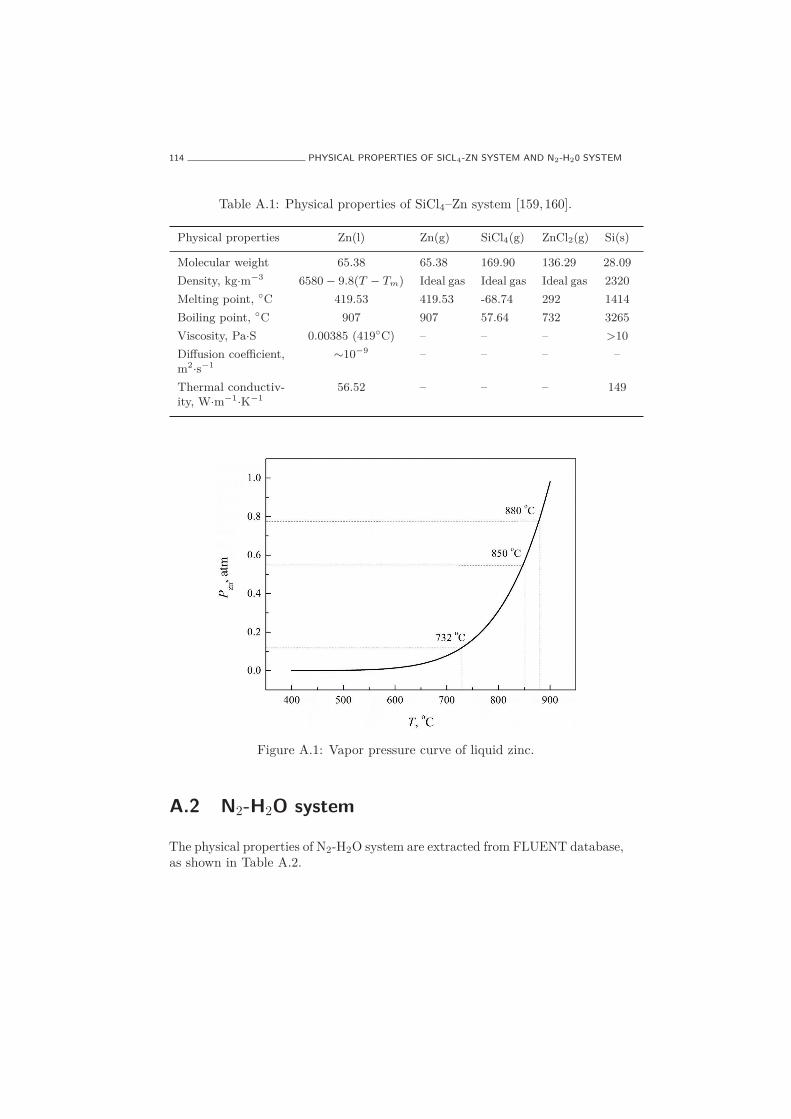
114 PHYSICAL PROPERTIES OF SICL4-ZN SYSTEM AND N2-H20 SYSTEM

Table A.1: Physical properties of SiCl4–Zn system [159,160].

Physical properties Zn(l) Zn(g) SiCl4(g) ZnCl2(g) Si(s)

Molecular weight 65.38 65.38 169.90 136.29 28.09

Density, kg·m−3 6580 − 9.8(T − Tm) Ideal gas Ideal gas Ideal gas 2320

Melting point, C 419.53 419.53 -68.74 292 1414

Boiling point, C 907 907 57.64 732 3265

Viscosity, Pa·S 0.00385 (419C) – – – >10

Diffusion coefficient,m2

·s−1

∼10−9 – – – –

Thermal conductiv-ity, W·m−1

·K−1

56.52 – – – 149

Figure A.1: Vapor pressure curve of liquid zinc.

A.2 N2-H2O system

The physical properties of N2-H2O system are extracted from FLUENT database,as shown in Table A.2.

N2-H2O SYSTEM 115

Table A.2: The physical properties of N2-H2O system.

Physical properties H2O(l) N2(g) H2O(g)

Molecular weight 18 28 18

Density, kg·m−3 997 1.185 0.554

Melting point, C 0 -210 0

Boiling point, C 100 -196 100

Viscosity, Pa·S 8.94 × 10−9 1.66 × 10−5 1.34 × 10−5

Diffusion coefficient, m2·s−1 – 2.88 × 10−5 2.88 × 10−5

Thermal conductivity, W·m−1·K−1 0.60 0.024 0.0261

The experimental values for saturated vapor pressure of liquid water can beexpressed as [161]:

p = exp(20.386 − 5132/T ) (A.2)

Where p in mmHg, T is the temperature in Kelvin. The vapor pressure equation(A.2) is shown in Figure A.2.

Figure A.2: Vapor pressure curve of liquid water.

Appendix B

The Illustration of Interface

mass transfer model

• Find interface grid cells.

Figure B.1: The illustration of interface grid cells for mass transfer.

117

118 THE ILLUSTRATION OF INTERFACE MASS TRANSFER MODEL

• Calculate interface area A.

Figure B.2: The two area expressions for triangle interface(I) and trapezoid(II), respectively. l is the grid cell length.

More details can be found in the UDF.

THE ILLUSTRATION OF INTERFACE MASS TRANSFER MODEL 119

120 THE ILLUSTRATION OF INTERFACE MASS TRANSFER MODEL

Bibliography

[1] J.R. Davis. Aluminum and Aluminum Alloys. page 210. ASMInternational, 1993.

[2] Dipak Mazumdar and James W. Evans. Modeling of SteelmakingProcesses. page 85. CRC Press, 2009.

[3] N. Kantarci, F. Borak, and K.O. Ulgen. Bubble column reactors. ProcessBiochemistry, 40:2263–2283, 2005.

[4] M. van Sint Annaland, N.G. Deen, and J.A.M. Kuipers. Multi-levelmodelling of dispersed gas-liquid two-phase flows. In Bubbly Flows, pages139–157. Springer, 2004.

[5] G.B. Marin. Multiscale Simulation and Design. volume 40, page 24.Academic Press, 2011.

[6] B. Aboulhasanzadeh, S. Thomas, M. Taeibi-Rahni, and G. Tryggvason.Multiscale computations of mass transfer from buoyant bubbles. ChemicalEngineering Science, 75:456–467, 2012.

[7] I. Roghair. Direct Numerical Simulations of Hydrodynamics and MassTransfer in Dense Bubbly Flows. PhD thesis, Technische UniversiteitEindhoven, 2012.

[8] K. Ono and T. Matsushima. On the production of pure silicon. The 61stReport of Research Institute of Mineral Dressing and Metallurgy, pages477–496, 1954.

[9] V. Roig, M. Roudet, F. Risso, and A. Billet. Dynamics of a high-Reynolds-number bubble rising within a thin gap. Journal of Fluid Mechanics,707:444–466, 2012.

121

122 BIBLIOGRAPHY

[10] W.G. Davenport, A. V. Bradshaw, and F.D. Richardson. Behavior ofspherical cap bubbles in liquid metals. Journal of the Iron and SteelInstitute, 205:1034–1042, 1967.

[11] J. Szekely. Fluid Flow Phenomena In Metals Processing. Elsevier Science,2012.

[12] Paneni and W.G. Davenport. Dynamics of bubbles in liquid metals: twodimensional experiments. Metallurgical Transactions, 1:297–297, 1970.

[13] Schwerdtfeger, K. Velocity of rise of argon bubbles in mercury. ChemicalEngineering Science, 23:937–938, 1968.

[14] S. Eckert, W. Witke, and G. Gerbeth. A new mechano-optical techniqueto measure local velocities in opaque fluids. Flow Measurement andInstrumentation, 11:71–78, 2000.

[15] A.C. Mikrovas and S.A. Argyropoulos. Measurement of velocity in high-temperature liquid metals. Metallurgical Transactions B, 24:1009–1022,1993.

[16] S. Eckert, G. Gerbeth, and V.I. Melnikov. Velocity measurements at hightemperatures by ultrasound Doppler velocimetry using an acoustic waveguide. Experiments in Fluids, 35:381–388, 2003.

[17] Q. Fu. Optimization of chlorine fluxing process for magnesium removalfrom molten aluminum. Ph.d thesis, University of California, Berkeley„1998.

[18] M. Iguchi, T. Nakatani, and H. Kawabata. Development of a multineedleelectroresistivity probe for measuring bubble characteristics in moltenmetal baths. Metallurgical and Materials Transactions B, 28:409–416,1997.

[19] Y. Saito, X. Shen, K. Mishima, and M. Matsubayashi. Shape measurementof bubble in a liquid metal. Nuclear Instruments and Methods in PhysicsResearch, 605:192–196, 2009.

[20] B. Klaasen. Gas bubbles in liquid metal in a Hele-Shaw cell a mesocropicstudy. Ph.d thesis, University of Leuven, 2014.

[21] J.K. Brimacombe, E.S. Stratigakos, and P. Tarassoff. Mass transferbetween a horizontal, submerged gas jet and a liquid. MetallurgicalTransactions, 5:763–771, 1974.

BIBLIOGRAPHY 123

[22] J.R.F. Guedes de Carvalho, F.A.N. Rocha, M.I. Vasconcelos, M.C.M.Silva, and F.A.R. Oliveira. Mass transfer during bubbling in single andmulti-orifice absorbers. Chemical Engineering Science, 41:1987–1994,1986.

[23] R.M. Davies and G. Taylor. The mechanics of large bubbles rising throughextended liquids and through liquids in tubes. Proceedings of the RoyalSociety of London A, 200:375–390, 1950.

[24] W.G. Davenport, F.D. Richardson, and A.V. Bradshaw. Spherical capbubbles in low density liquids. Chemical Engineering Science, 22:1221–1235, 1967.

[25] R. Clift, J.R. Grace, and M.E. Weber. Bubbles, Drops, and Particles.pages 1–240. Acedemic press, 1978.

[26] A.A. Kulkarni and J.B. Joshi. Bubble Formation and Bubble Rise Velocityin Gas - Liquid Systems : A Review. Industrial and Engineering ChemistryResearch, 44:5873–5931, 2005.

[27] F. Durst, B. Schönung, K. Selanger, and M. Winter. Bubble-driven liquidflows. Journal of Fluid Mechanics, 170:53–82, 1986.

[28] M.I. Urseanu. Scaling up bubble column reactors. Ph.d thesis, UniversiteitVan Amsterdam, 2000.

[29] M. Wu and M. Gharib. Experimental studies on the shape and path ofsmall air bubbles rising in clean water. Physics of Fluids, 14:L49–L52,2002.

[30] P.C. Duineveld. The rise velocity and shape of bubbles in pure water athigh Reynolds number. Journal of Fluid Mechanics, 292:325–332, 1995.

[31] K. Ellingsen and F. Risso. On the rise of an ellipsoidal bubble in water:oscillatory paths and liquid-induced velocity. Journal of Fluid Mechanics,440:235–268, 2001.

[32] W.L. Shew, S. Poncet, and J.F. Pinton. Force measurements on risingbubbles. Journal of Fluid Mechanics, 569:51–60, 2006.

[33] G. Mougin and J. Magnaudet. Path instability of a rising bubble. PhysicalReview Letters, 88:014502, 2002.

[34] T. Sanada, M. Shirota, and M. Watanabe. Bubble wake visualization byusing photochromic dye. Chemical Engineering Science, 62:7264–7273,2007.

124 BIBLIOGRAPHY

[35] C. Bru. Structure and dynamics of the wake of bubbles and its relevancefor bubble interaction. Physics of Fluids, 11:1781–1796, 1999.

[36] G.K. Batchelor. The stability of a large gas bubble rising through liquid.Journal of Fluid Mechanics, 184:399–422, 1987.

[37] K. Tsuchiya and L. Fan. Near-wake structure of a single gas bubble in atwo-dimensional liquid-solid fluidized bed: vortex shedding and wake sizevariation. Chemical Engineering Science, 43:1167–1181, 1988.

[38] P.G. Saffman. On the rise of small air bubbles in water. Journal of FluidMechanics, 1:249–275, 1956.

[39] H.D. Mendelson. The prediction of bubble terminal velocities from wavetheory. AIChE Journal, 13:250–253, 1967.

[40] G. Bozzano and M. Dente. Shape and terminal velocity of single bubblemotion: a novel approach. Computer aided chemical engineering, 8:649–654, 2000.

[41] D. Rodrigue. A general correlation for the rise velocity of single gasbubbles. The Canadian Journal of Chemical Engineering, 82:382–386,2004.

[42] M. Stöhr, J. Schanze, and A. Khalili. Visualization of gas-liquid masstransfer and wake structure of rising bubbles using pH-sensitive PLIF.Experiments in Fluids, 47:135–143, 2009.

[43] A.B. Newman. The Drying of Porous Solids: Diffusion Calculations, andDiffusion and Surface Emission Equations. Transactions of the AmericanInstitute of Chemical Engineers, 27:203–211, 1931.

[44] R. Kronig and J.C. Brink. On the theory of extraction from fallingdroplets. Applied Scientific Research, 2:142–154, 1950.

[45] L.E. Johns and R.B. Beckmann. Mechanism of dispersed phase masstransfer in visous, single drop extraction system. AIChE Journal, 12:10–16,1966.

[46] H. Watada, A.E. Hamielec, and A.I. Johnson. A theoretical study ofmass transfer with chemical reaction in drops. The Canadian Journal ofChemical Engineering, 48:255–261, 1970.

[47] M. Filla, J.F. Davidson, J.F. Bates, and M.A. Eccles. Gas phase controlledmass transfer from a bubble. Chemical Engineering Science, 31:359–367,1976.

BIBLIOGRAPHY 125

[48] T. Taha and Z.F. Cui. Hydrodynamics of slug flow inside capillaries.Chemical Engineering Science, 59:1181–1190, 2004.

[49] N.E. Zaritzky and A. Calvelo. Internal mass transfer coefficient withinsingle bubbles theory and experiment. The Canadian Journal of ChemicalEngineering, 57:58–64, 1979.

[50] C.-W. Park and G.M. Homsy. Two-phase displacement in Hele Shaw cells:theory. Journal of Fluid Mechanics, 139:291–308, 1984.

[51] B. Sandnes, E.G. Flekkoy, H.A. Knudsen, K.J. Maloy, and H. See. Patternsand flow in frictional fluid dynamics. Nature communications, 2:288, 2011.

[52] J.W.M. Bush. The anomalous wake accompanying bubbles rising in a thingap: a mechanically forced Marangoni flow. Journal of Fluid Mechanics,352:283–303, 1997.

[53] T. Maxworthy. The nonlinear growth of a gravitationally unstable interfacein a Hele-Shaw cell. Journal of Fluid Mechanics, 177:207–232, 1987.

[54] G.I. Taylor and Saffman P.G. A note on the motion of bubbles in aHele-Shaw cell and porous medium. The Quarterly Journal of Mechanicsand Applied Mathematics, 12:265–279, 1959.

[55] S. Tanveer. The effect of surface tension on the shape of a Hele-CShawcell bubble. Physics of Fluids, 29:3537–3548, 1986.

[56] T. Maxworthy. Bubble formation, motion and interaction in a Hele-Shawcell. Journal of Fluid Mechanics, 173:95–114, 1986.

[57] A.R. Kopf-Sill and G.M. Homsy. Nonlinear unstable viscous fingers inHele-Shaw flows. I. Experiments. Physics of Fluids, 31:242–249, 1988.

[58] E. Kelley and M. Wu. Path instabilities of rising air bubbles in a Hele-Shawcell. Physical review letters, 79:1265–1268, 1997.

[59] M. Kawaguchi, S. Niga, N. Gou, and K. Miyake. Buoyancy-driven pathinstabilities of bubble rising in simple and polymer solutions of Hele-Shawcell. Journal of the Physical Society of Japan, 75:124401, 2006.

[60] H. Kozuka, Y. Ikeda, and M. Kawaguchi. Path instabilities of bubblerising in polymer solutions of Hele-Shaw cell. Journal of the PhysicalSociety of Japan, 78:114604, 2009.

[61] M. Yamamoto and M. Kawaguchi. Differences in path instabilities betweena bubble rising in water and in aqueous polymer solution in a Hele-Shawcell in the transient and steady states. Journal of Dispersion Science andTechnology, 32:1445–1451, 2011.

126 BIBLIOGRAPHY

[62] B. Klaasen, F. Verhaeghe, B. Blanpain, and J. Fransaer. A study of gasbubbles in liquid mercury in a vertical Hele-Shaw cell. Experiments inFluids, 55:1652, 2014.

[63] B. Klaasen, F. Verhaeghe, B. Blanpain, and J. Fransaer. ObservingNitrogen Bubbles in Liquid Zinc in a Vertical Hele-Shaw Cell. Metallurgicaland Materials Transactions B, pages 1–14, 2015.

[64] M. van Sint Annaland, W. Dijkhuizen, N.G. Deen, and J.A.M. Kuipers.Numerical simulation of behavior of gas bubbles using a 3-D front-trackingmethod. AIChE Journal, 52:99–110, 2006.

[65] William F Noh and Paul Woodward. Slic (simple line interface calculation).In Proceedings of the Fifth International Conference on Numerical Methodsin Fluid Dynamics June 28–July 2, 1976 Twente University, Enschede,pages 330–340. Springer, 1976.

[66] J.U. Brackbill, D.B. Kothe, and C Zemach. A continuum method formodeling surface tension. Journal of Computational Physics, 100:335–354,1991.

[67] W.J. Rider and D.B. Kothe. Reconstructing Volume Tracking. Journalof Computational Physics, 141:112–152, 1998.

[68] S. Osher and J.A. Sethian. Fronts propagating with curvature dependentspeed: Algorithms based on Hamilton-Jacobi formulations. Journal ofComputational Physics, 79:12–49, 1987.

[69] K.B. Deshpande and W.B. Zimmerman. Simulation of interfacial masstransfer by droplet dynamics using the level set method. ChemicalEngineering Science, 61:6486–6498, 2006.

[70] Z. Yu and L.S. Fan. Direct simulation of the buoyant rise of bubbles ininfinite liquid using level set method. The Canadian Journal of ChemicalEngineering, 86:267–275, 2008.

[71] E. Olsson and G. Kreiss. A conservative level set method for two phaseflow. Journal of Computational Physics, 210:225–246, 2005.

[72] E. Olsson, G. Kreiss, and S. Zahedi. A conservative level set method fortwo phase flow II. Journal of Computational Physics, 225:785–807, 2007.

[73] D. Enright, R. Fedkiw, J. Ferziger, and I. Mitchell. A hybrid particle levelset method for improved interface capturing. Journal of ComputationalPhysics, 183(1):83–116, 2002.

BIBLIOGRAPHY 127

[74] G. Tryggvason, B. Bunner, A. Esmaeeli, D. Juric, N. Al-Rawahi,W. Tauber, J. Han, S. Nas, and Y.-J. Jan. A front-tracking method forthe computations of multiphase flow. Journal of Computational Physics,169:708–759, 2001.

[75] G. Tryggvason, R. Scardovelli, and S. Zaleski. Direct NumericalSimulations of Gas-Liquid Multiphase Flows. page 95. CambridgeUniversity Press, 2011.

[76] R. Singh and W. Shyy. Three-dimensional adaptive Cartesian grid methodwith conservative interface restructuring and reconstruction. Journal ofComputational Physics, 224:150–167, 2007.

[77] M. van Sint Annaland, N.G. Deen, and J.A.M. Kuipers. Numericalsimulation of gas bubbles behaviour using a three-dimensional volume offluid method. Chemical Engineering Science, 60:2999–3011, 2005.

[78] I.R. Park, K.S. Kim, J. Kim, and S.H. Van. A volume-of-fluid methodfor incompressible free surface flows. International Journal for NumericalMethods in Fluids, 61:1331–1362, 2009.

[79] G. Mougin and J. Magnaudet. Wake-induced forces and torques on azigzagging/spiralling bubble. Journal of Fluid Mechanics, 567:185–194,2006.

[80] R. Krishna and J.M. Van Baten. Simulating the motion of gas bubbles ina liquid. Nature, 398:208–208, 1999.

[81] D. Gaudlitz and N.A. Adams. Numerical investigation of rising bubblewake and shape variations. Physics of Fluids, 21:122102, 2009.

[82] J. Zhang and M.J. Ni. Direct simulation of single bubble motion undervertical magnetic field: Paths and wakes. Physics of Fluids, 26:102102,2014.

[83] M. Kroger, A. Alke, D. Bothe, and H. Warnecke. A vof-based approach forthe simulation of reactive mass transfer from rising bubbles. FortschrittBerichte-VDI Reihe 3 Verfahrenstechnik, 883:290, 2007.

[84] A.A. Ganguli and E.Y. Kenig. A CFD-based approach to the interfacialmass transfer at free gas¨Cliquid interfaces. Chemical Engineering Science,66:3301–3308, 2011.

[85] G. Pianet, S. Vincent, J. Leboi, J.P. Caltagirone, and M. Anderhuber.Simulating compressible gas bubbles with a smooth volume tracking 1-Fluid method. International Journal of Multiphase Flow, 36:273–283,2010.

128 BIBLIOGRAPHY

[86] A.R. Kopf-Sill and G.M. Homsy. Bubble motion in a Hele-CShaw cell.Physics of Fluids, 31:18–26, 1988.

[87] S.R.K. Maruvada and C.-W. Park. Retarded motion of bubbles in Hele-Shaw cells. Physics of Fluids, 8:3229–3233, 1996.

[88] W. Eck and J. Siekmann. On bubble motion in a Hele-Shaw cell, apossibility to study 2-phase flows under reduced gravity. Ingenieur-Archiv,47:153–168, 1978.

[89] R. Collins. A simple model of the plane gas bubble in a finite liquid.Journal of Fluid Mechanics, 22:763–771, 1966.

[90] F. Riegels. Zur Kritik des Hele-Shaw-Versuchs. Zeitschrift fur AngewandteMathematik und Mechanik, 18:95–106, 1938.

[91] S.G. Huisman, P. Ern, and V. Roig. Interaction and coalescence of largebubbles rising in a thin gap. Physical Review E, 85:027302, 2012.

[92] J.W.M. Bush and I. Eames. Fluid displacement by high Reynolds numberbubble motion in a thin gap. International Journal of Multiphase Flow,24:411–430, 1998.

[93] D. Ma, M. Liu, Y. Zu, and C. Tang. Two-dimensional volume of fluidsimulation studies on single bubble formation and dynamics in bubblecolumns. Chemical Engineering Science, 72:61–77, 2012.

[94] W. Boos and A. Thess. Thermocapillary flow in a Hele-Shaw cell. Journalof Fluid Mechanics, 352:305–330, 1997.

[95] P. Gondret and M. Rabaud. Shear instability of two-fluid parallel flow ina Hele-Shaw cell. Physics of Fluids, 9:3267–3274, 1997.

[96] A. Tatulchenkov and A. Cebers. Complex bubble dynamics in a verticalHele-Shaw cell. Physics of Fluids, 17:107103, 2005.

[97] N. Jarrige, I. Bou Malham, J. Martin, N. Rakotomalala, D. Salin, andL. Talon. Numerical simulations of a buoyant autocatalytic reaction frontin tilted Hele-Shaw cells. Physical Review E - Statistical, Nonlinear, andSoft Matter Physics, 81:066311, 2010.

[98] R. Krishna and J.M. Van Baten. Rise characteristics of gas bubbles ina 2D rectangular column: VOF simulation vs experiment. InternationalCommunications in Heat and Mass Transfer, 26:965–974, 1999.

[99] J.M. Van Baten and R. Krishna. CFD simulations of mass transfer fromTaylor bubbles rising in circular capillaries. Chemical Engineering Science,59:2535–2545, 2004.

BIBLIOGRAPHY 129

[100] G.S. Beavers, E.M. Sparrow, and R.A. Magnuson. Experiments on thebreakdown of laminar flow in a parallel-plate channel. InternationalJournal of Heat and Mass Transfer, 13:809–815, 1970.

[101] I. Lunati and D. Or. Gravity-driven slug motion in capillary tubes. Physicsof Fluids, 21:052003, 2009.

[102] M. Seifollahi, E. Shirani, and N. Ashgriz. An improved method forcalculation of interface pressure force in PLIC-VOF methods. EuropeanJournal of Mechanics B, 27:1–23, 2008.

[103] S.Y. Lin, Y.H. Chin, C.M. Wu, J.F. Lin, and Y.C. Chen. A pressurecorrection-volume of fluid method for simulation of two-phase flows.International Journal for Numerical Methods in Fluids, 68:181–195, 2010.

[104] D.L. Youngs. Time-dependent multi-material flow with large fluiddistortion. pages 27–39. Academic Press, 1982.

[105] V. Kolár. Vortex identification: New requirements and limitations.International Journal of Heat and Fluid Flow, 28:638–652, 2007.

[106] J. Zhou, R.J. Adrian, S. Balachandar, and T.M. Kendall. Mechanisms forgenerating coherent packets of hairpin vortices in channel flow. Journalof Fluid Mechanics, 387:353–396, 1999.

[107] B.G.M. van Wachem and J.C. Schouten. Experimental validation of 3-Dlagrangian VOF model: Bubble shape and rise velocity. AIChE Journal,48:2744–2753, 2002.

[108] M.R. Ansari and M.E. Nimvari. Bubble viscosity effect on internalcirculation within the bubble rising due to buoyancy using the levelset method. Annals of Nuclear Energy, 38:2770–2778, 2011.

[109] K.D. Danov, D.S. Valkovska, and P.A. Kralchevsky. Hydrodynamicinstability and coalescence in trains of emulsion drops or gas bubblesmoving through a narrow capillary. Journal of Colloid and InterfaceScience, 267:243–258, 2003.

[110] E. Bouche, V. Roig, F. Risso, and A.-M. Billet. Homogeneous swarm ofhigh-Reynolds-number bubbles rising within a thin gap. Part 1. Bubbledynamics. Journal of Fluid Mechanics, 704:211–231, 2012.

[111] G.M. Lazarek and H. Littman. The pressure field due to a large circularcapped air bubble rising in water. Journal of Fluid Mechanics, 66:673–687,1974.

130 BIBLIOGRAPHY

[112] W.F. Bessler and H. Littman. Experimental studies of wakes behindcircularly capped bubbles. Journal of Fluid Mechanics, 185:137–151,1987.

[113] X. Wang, B. Klaasen, J. Degrève, B. Blanpain, and F. Verhaeghe.Experimental and numerical study of buoyancy-driven single bubbledynamics in a vertical Hele-Shaw cell Experimental and numerical studyof buoyancy-driven single bubble dynamics in a vertical Hele-Shaw cell.Physics of Fluids, 26:123303, 2014.

[114] J.H. Hills. The two-dimensional elliptical cap bubble. Journal of FluidMechanics, 68:503–512, 1975.

[115] Y. Yang and H. Levine. Spherical cap bubbles. Journal of Fluid Mechanics,235:73–87, 1992.

[116] K. Raghunathan, S. Kumar, and L.-S. Fan. Pressure distribution andvortical structure in the wake behind gas bubbles in liquid and liquid-solidsystems. International Journal of Multiphase Flow, 18:41–50, 1992.

[117] L.-S. Fan and K. Tsuchiya. Bubble wake dynamics in liquids and liquid-solid suspensions. page 71. Butterworths-Heinemann, 1990.

[118] L. Han and M.H. Al-Dahhan. Gas-liquid mass transfer in a highpressure bubble column reactor with different sparger designs. ChemicalEngineering Science, 62:131–139, 2007.

[119] T. Maxworthy. A note on the existence of wakes behind large, risingbubbles. Journal of Fluid Mechanics, 27:367–368, 1967.

[120] J.Y. Parlange. Spherical cap bubbles with laminar wakes. Journal ofFluid Mechanics, 37:257–263, 2006.

[121] A.W.G. De Vries, A. Biesheuvel, and L. Van Wijngaarden. Notes on thepath and wake of a gas bubble rising in pure water. International Journalof Multiphase Flow, 28:1823–1835, 2002.

[122] K. Sakakibara, M. Yamada, Y. Miyamoto, and T. Saito. Measurementof the surrounding liquid motion of a single rising bubble using a Dual-Camera PIV system. Flow Measurement and Instrumentation, 18:211–215,2007.

[123] Z. Liu and Y. Zheng. PIV study of bubble rising behavior. PowderTechnology, 168:10–20, 2006.

BIBLIOGRAPHY 131

[124] M. Roudet, A.M. Billet, F. Risso, and V. Roig. PIV with volume lightingin a narrow cell: An efficient method to measure large velocity fields ofrapidly varying flows. Experimental Thermal and Fluid Science, 35:1030–1037, 2011.

[125] Z. Liu, Y. Zheng, L. Jia, and Q. Zhang. Study of bubble induced flowstructure using PIV. Chemical Engineering Science, 60:3537–3552, 2005.

[126] R. Zenit and J. Magnaudet. Measurements of the streamwise vorticity inthe wake of an oscillating bubble. International Journal of MultiphaseFlow, 35:195–203, 2009.

[127] R. Zenit and J. Magnaudet. Path instability of rising spheroidal airbubbles: A shape-controlled process. Physics of Fluids, 20:061702, 2008.

[128] J. Magnaudet and G. Mougin. Wake instability of a fixed spheroidalbubble. Journal of Fluid Mechanics, 572:311–337, 2007.

[129] Xue Wang, Bart Klaasen, Jan Degrève, Bart Blanpain, and FrederikVerhaeghe. Volume-of-fluid simulations of bubble dynamics in a verticalHele-Shaw cell. Submitted to Physics of Fluids.

[130] M.T. Pauken. An experimental investigation of combined turbulent freeand forced evaporation. Experimental Thermal and Fluid Science, 18:334–340, 1998.

[131] I.W. Eames, N.J. Marr, and H. Sabir. The evaporation coefficient of water:a review. International Journal of Heat and Mass Transfer, 40:1963–2973,1997.

[132] E. Sartori. A critical review on equations employed for the calculationof the evaporation rate from free water surfaces. Solar Energy, 68:77–89,2000.

[133] P. Rahimi and C.A. Ward. Kinetics of evaporation: statistical rate theoryapproach. International Journal of Thermodynamics, 8:1–14, 2005.

[134] L.E. Scriven. On the dynamics of phase growth. Chemical EngineeringScience, 50:1–13, 1959.

[135] J. Wang, P. Lu, Z. Wang, C. Yang, and Z. Mao. Numerical simulation ofunsteady mass transfer by the level set method. Chemical EngineeringScience, 63:3141–3151, 2008.

[136] P. Lu, Z. Wang, C. Yang, and Z. Mao. Experimental investigation andnumerical simulation of mass transfer during drop formation. ChemicalEngineering Science, 65:5517–5526, 2010.

132 BIBLIOGRAPHY

[137] Z. Wang, P. Lu, Y. Wang, C. Yang, and Z. Mao. ExperimentalInvestigation and Numerical Simulation of Marangoni Effect Inducedby Mass Transfer during Drop Formation. AIChE Journal, 59:4424–4439,2013.

[138] G. Strotos, M. Gavaises, A. Theodorakakos, and G. Bergeles. Numericalinvestigation of the evaporation of two-component droplets. Fuel, 90:1492–1507, 2011.

[139] D. Sun, J. Xu, and L. Wang. Development of a vapor¨Cliquid phasechange model for volume-of-fluid method in FLUENT. InternationalCommunications in Heat and Mass Transfer, 39:1101–1106, 2012.

[140] W. Lee, G. Son, and H.Y. Yoon. Direct numerical simulation of flowboiling in a finned microchannel. International Communications in Heatand Mass Transfer, 39:1460–1466, 2012.

[141] R. Banerjee. Turbulent conjugate heat and mass transfer from the surfaceof a binary mixture of ethanol/iso-octane in a countercurrent stratifiedtwo-phase flow system. International Journal of Heat and Mass Transfer,51:5958–5974, 2008.

[142] J.B. Haelssig, A.Y. Tremblay, J. Thibault, and S.G. Etemad.Direct numerical simulation of interphase heat and mass transfer inmulticomponent vapour-liquid flows. International Journal of Heat andMass Transfer, 53:3947–3960, 2010.

[143] A. Hassanvand and S.H. Hashemabadi. Direct numerical simulation ofinterphase mass transfer in gas ¨C liquid multiphase systems. InternationalCommunications in Heat and Mass Transfer, 38:943–950, 2011.

[144] D.G. Kröger and G.R. Branfield. Evaporation from a Water Surface :Theory and Experiment. R&D Journal of the South African Institutionof Mechanical Engineering, 23:5–11, 2007.

[145] A. Alke, D. Bothe, M. Kroeger, and H.J. Warnecke. VOF-basedsimulation of conjugate mass transfer from freely moving fluid particles.Computational Methods in Multiphase Flow V, pages 157–168, 2009.

[146] S. Hardt and F. Wondra. Evaporation model for interfacial flows basedon a continuum-field representation of the source terms. Journal ofComputational Physics, 227:5871–5895, 2008.

[147] S. Jeon, S. Kim, and G. Park. Numerical study of condensing bubble insubcooled boiling flow using volume of fluid model. Chemical EngineeringScience, 66:5899–5909, 2011.

BIBLIOGRAPHY 133

[148] H. Marschall, K. Hinterberger, C. Schüler, F. Habla, and O. Hinrichsen.Numerical simulation of species transfer across fluid interfaces in free-surface flows using OpenFOAM. Chemical Engineering Science, 78:111–127, 2012.

[149] G. Strotos, M. Gavaises, A. Theodorakakos, and G. Bergeles. Numericalinvestigation on the evaporation of droplets depositing on heated surfacesat low Weber numbers. International Journal of Heat and Mass Transfer,51:1516–1529, 2008.

[150] S. Popov, A. Melling, F. Durst, and C.A. Ward. Apparatus forinvestigation of evaporation at free liquid-vapour interfaces. InternationalJournal of Heat and Mass Transfer, 48:2299–2309, 2005.

[151] R. Marek and J. Straub. Analysis of the evaporation coefficient and thecondensation coefficient of water. International Journal of Heat and MassTransfer, 44:39–53, 2001.

[152] T.H. Yang and C. Pan. Molecular dynamics simulation of a thin waterlayer evaporation and evaporation coefficient. International Journal ofHeat and Mass Transfer, 48:3516–3526, 2005.

[153] V.K. Badam, V. Kumar, F. Durst, and K. Danov. Experimentaland theoretical investigations on interfacial temperature jumps duringevaporation. Experimental Thermal and Fluid Science, 32:276–292, 2007.

[154] U.D. Kück, M. Schlüter, and N. Räbiger. Analyse des grenzschichtnahenStofftransports an frei aufsteigenden Gasblasen. Chemie Ingenieur Technik,81:1599–1606, 2009.

[155] T. Iida and R.I.L. Guthrie. The physical properties of liquid metals.Clarendon Press, 1988.

[156] Ishino T. Matstumoto, A. Manufacture of high-purity silicon. I.Disproportionation reaction of silicon and silicon tetrachloride. KogyoKagaku Zasshi, 6:262–265, 1965.

[157] R.C. Reid, J.M. Prausnitz, and B.E. Poling. The properties of gases andliquids. page 90. McGraw Hill Book Co.,New York, NY, 1977.

[158] Y.K. Rao. Stoichiometry and thermodynamics of metallurgical processes .Cambridge University Press, 1985.

[159] B. Sylvan. Liquid metals chemistry and physics. page 451. Marcel Dekker,New York, 1972.

[160] R.N. Lyon. Liquid-metal handbooks. page 43. U.S. Government, 1952.

134 BIBLIOGRAPHY

[161] W.M. Haynes. CRC Handbook of Chemistry and Physics. CRC Press,2012.

Curriculum Vitae

Xue Wang

Date of birth: 20 January 1982

Place of birth: Sichuan, China

Email address: [email protected]

Education

• 09. 2010–04. 2015: PhD student in Engineering ScienceDepartment of Materials Engineering (MTM)University of Leuven (KU Leuven)Belgium.

• 09. 2004–07. 2007:Master in Chemical TechnologyKey laboratory of Green Process and EngineeringInstitute of Process Engineering, ChineseAcademy of SciencesChina.

• 09. 2000–07. 2004:Bachelor in Metallurgical TechnologyCollege of Chemical EngineeringSichuan UniversityChina.

Work experience

• 07. 2007–09. 2010:China Petroleum Chemical CorporationChina National Petroleum CorporationChina.

135

List of Publications

Articles in internationally reviewed journals

[1] X. Wang, B. Klaasen, J. Degrève, B. Blanpain, F. Verhaeghe. Experimentaland numerical study of buoyancy-driven single bubble dynamics in a verticalHele-Shaw cell. Physics of Fluids, 26 (2014) 123303.

[2] X. Wang, B. Klaasen, J. Degrève, B. Blanpain, F. Verhaeghe. Volume-of-fluid simulations of bubble dynamics in a vertical Hele-Shaw cell. (Submittedto Physics of Fluids)

[3] X. Wang, B. Klaasen, J. Degrève, A. Mahulkar, G. Heynderickx, M.Reyniers, B. Blanpain, F. Verhaeghe. A quantitative modelling of two-dimensional rising bubble dynamics: drag coefficient and bubble wake. (Inpreparation)

[4] X. Wang, A. Mahulkar, B. Klaasen, J. Degrève, M. Reyniers, B. Blanpain,F. Verhaeghe. Numerical simulation of bubble dynamics and evaporation. (Inpreparation)

Papers at international conferences, published in full in proceedings

[1] X. Wang, B. Klaasen, J. Degrève, B. Blanpain, F. Verhaeghe. Twodimensional numerical simulation of bubble dynamics in a vertical Hele-Shawcell. CFD2014: Proceedings of 10th International Conference on CFD in Oiland Gas, Metallurgical and Process Industries, SINTEF, Trondheim, Norway,Jun 17-19, 2014. pp. 687-694.

137

FACULTY OF ENGINEERING SCIENCE

DEPARTMENT OF MATERIALS ENGINEERING (MTM)

HIGH TEMPERATURE PROCESSES AND INDUSTIAL ECOLOGY

Kasteelpark Arenberg 44 bus 2450

B-3001 Heverlee

[email protected]

http://www.mtm.kuleuven.be

Numerical Simulation of Two-Dimensional Bubble Dynamics and ...

Documents

Transcript of Numerical Simulation of Two-Dimensional Bubble Dynamics and ...