Numerical Simulation and Subgrid-Scale Modeling of Mixingand Wall-Bounded Turbulent Flows

Thesis by

Daniel Chung

In Partial Fulfillment of the Requirements

for the Degree of

Doctor of Philosophy

California Institute of Technology

Pasadena, California

2009

(Defended May 1, 2009)

ii

c© 2009

Daniel Chung

All Rights Reserved

iii

Acknowledgements

I would like to thank my advisor Professor Dale Pullin who led our discussions with considerable skill

and gave me much-needed encouragement in what turned out to be a challenging research project—

I will never forget the first time I saw his blackboard illustration that was meant to describe my

progress: a point on a hill located just before it slopes downward. Little did we know that the

illustration had to make frequent appearances for another two years. Dale taught me the value of

answering in the wrong way the right questions as opposed to answering in the right way the wrong

questions; it was after I understood this principle that my research approach matured.

I would also like to express my appreciation to my thesis committee members, Professors Oscar

Bruno, Tim Colonius, Mory Gharib, and Beverley McKeon, who took the time to read my thesis

and offered suggestions that improved my thesis.

Thanks to everybody at GALCIT and Caltech, the research playground of the world. It was a

privilege to associate with some of the smartest and funnest people who have and will continue to

shape the future of our world. I would specifically like to thank the various members of the Iris and

Puckett laboratories, Ivan, Michio, Richard, Manuel, Mike and Karen, Andrew, and Yue. I would

also like to thank my friends in the wider Caltech community for the memorable mountain-biking

trips, beach days, and late-night parties: Waheb, Rogier, Chris and Lydia, Christian and Jennifer,

Giselle, Vala, Sean and Marta, Liliya, Anusha, Aaron, Maria, Raviv, Angel, Alex, and Melanie.

Special thanks to Bill Bing, who ran the Caltech Monday Jazz Band with energy and passion—

drumming for the Caltech MJB was one of the highlights of my week.

Thanks to Professors Min Chong and Andrew Ooi at The University of Melbourne, who first got

me interested in fluid mechanics through their inspiring lectures and also gave me the opportunity

to perform undergraduate research with their group; my interactions at Melbourne with Matteo,

Keith, Anne, Malcolm, Jason, and Ronny instilled in me an appreciation for careful fluid mechanics

research.

I am also fortunate to associate with friends from the Art Center College of Design: Michelle,

Katherine, Eric, and Simone; I got to experience and learn about lots of awesome art.

Much thanks to Sumi and Maria who gave me the opportunity to bake with them at Europane;

it was one of the most rewarding experiences of my graduate life. It is fair to say that the only

iv

experiment in fluid mechanics that I performed during my graduate study is folding egg whites.

Thanks to Doctors David Hill and Carlos Pantano for conversations and e-mail exchanges that

assisted me in understanding various numerical issues that cropped up in my research.

All the present computations were carried out on the excellently administrated Shared Hetero-

geneous Cluster (SHC) at the Caltech CACR, with access kindly provided by ASCI (Professor Dan

Meiron) and PSAAP (Professor Michael Ortiz).

Thanks to Professor Beverley McKeon who gave us the idea for the material in chapter 5 during

the summer of 2008.

I wish to thank Professor J. Jimenez who provided DNS spectra from Reτ = 2 k channel flow,

and Doctors W. H.Cabot and A. W. Cook who provided DNS spectra from high-Re Rayleigh–Taylor

instability.

I would like to thank my parents, Edmund Chung and Goh Kwang Ging, as well as my brother,

Collin Chung, who gave me their unconditional love, support, and encouragement during the course

of my graduate study.

Finally, I thank God for giving me the undeserved opportunity to study at this amazing school—it

was a blast.

This work is partially supported by the NSF under grant CBET 0651754.

v

Abstract

We extend the idea of multiscale large-eddy simulation (LES), the underresolved fluid dynamical

simulation that is augmented with a physical description of subgrid-scale (SGS) dynamics. Using

a vortex-based SGS model, we consider two areas of specialization: active (buoyant) scalar mixing

and wall-bounded turbulence.

First, we develop a novel method to perform direct numerical simulation (DNS) of statistically

stationary buoyancy-driven turbulence by using the fringe-region technique within a triply periodic

domain, in which a mixing region is sandwiched between two fringes that supply the flow with

unmixed fluids—heavy on top of light. Spectra exhibit small-scale universality, as evidenced by

collapse in inner scales. A comparison with high-resolution DNS spectra from Rayleigh–Taylor

turbulence reveals some similarities.

We perform LES of this flow to show that a passive scalar SGS model can also be used in an

unstably stratified environment. LES spectra, including subgrid extensions, show good agreement

with DNS data. For stably stratified flows, we develop an active scalar SGS model by performing a

perturbation expansion in small Richardson numbers of the passive scalar SGS model to obtain an

expression for the SGS scalar flux that contains buoyancy corrections.

We then develop a wall model for LES in which the near-wall region is unresolved. A special

near-wall SGS model is constructed by averaging the streamwise momentum equation together with

an assumption of local–inner scaling, giving an ordinary differential equation for the local wall shear

stress that is coupled with the LES. An extended form of the stretched-vortex SGS model, which

incorporates the production of near-wall Reynolds shear stresses due to the winding of streamwise

momentum by near-wall attached SGS vortices, then provides a log relation for the off-wall LES

boundary conditions. A Karman-like constant is calculated dynamically as part of the LES. With this

closure we perform LES of turbulent channel flow for friction-velocity Reynolds numbers Reτ = 2k–

20 M. Results, including SGS-extended spectra, compare favorably with DNS at Reτ = 2 k, and

maintain an O(1) grid dependence on Reτ .

Finally, we apply the wall model to LES of long channels to capture effects of large-scale struc-

tures. Computed correlations are found to be consistent with recent experiments.

vi

Contents

List of Figures ix

List of Tables xi

1 Introduction 1

1.1 LES . . . . . . . . . . . . . . . . . . . . . . . . . . . . . . . . . . . . . . . . . . . . . 2

1.2 Vortex-Based SGS Model . . . . . . . . . . . . . . . . . . . . . . . . . . . . . . . . . 3

1.3 Plan of Thesis . . . . . . . . . . . . . . . . . . . . . . . . . . . . . . . . . . . . . . . . 4

2 DNS of Statistically Stationary Buoyancy-Driven Turbulence 5

2.1 Background . . . . . . . . . . . . . . . . . . . . . . . . . . . . . . . . . . . . . . . . . 5

2.2 Problem Description . . . . . . . . . . . . . . . . . . . . . . . . . . . . . . . . . . . . 7

2.2.1 Governing Equations . . . . . . . . . . . . . . . . . . . . . . . . . . . . . . . . 7

2.2.2 Consequences of Periodicity . . . . . . . . . . . . . . . . . . . . . . . . . . . . 8

2.2.3 Fringe-Region Forcing . . . . . . . . . . . . . . . . . . . . . . . . . . . . . . . 9

2.2.4 Mean Pressure Gradient . . . . . . . . . . . . . . . . . . . . . . . . . . . . . . 13

2.3 Solution Method . . . . . . . . . . . . . . . . . . . . . . . . . . . . . . . . . . . . . . 13

2.3.1 Alternative Lagrange Multiplier to Pressure . . . . . . . . . . . . . . . . . . . 13

2.3.2 Numerical Discretization . . . . . . . . . . . . . . . . . . . . . . . . . . . . . . 15

2.3.3 Code Validation . . . . . . . . . . . . . . . . . . . . . . . . . . . . . . . . . . 16

2.4 Results and Discussion . . . . . . . . . . . . . . . . . . . . . . . . . . . . . . . . . . . 17

2.4.1 Integral and Taylor Statistics . . . . . . . . . . . . . . . . . . . . . . . . . . . 20

2.4.2 Spectra . . . . . . . . . . . . . . . . . . . . . . . . . . . . . . . . . . . . . . . 22

2.4.3 Mole Fraction Probability Density Functions . . . . . . . . . . . . . . . . . . 25

3 LES and SGS Modeling of Active Scalar Mixing Flows 27

3.1 Background . . . . . . . . . . . . . . . . . . . . . . . . . . . . . . . . . . . . . . . . . 27

3.2 LES of Unstably Stratified Flow . . . . . . . . . . . . . . . . . . . . . . . . . . . . . 29

3.2.1 Filtered LES Equations and SGS Model . . . . . . . . . . . . . . . . . . . . . 29

vii

3.2.2 Subgrid Extensions of Planar Spectra . . . . . . . . . . . . . . . . . . . . . . 31

3.3 SGS Model for Stably Stratified Flows . . . . . . . . . . . . . . . . . . . . . . . . . . 37

3.3.1 Vortex-Based SGS Model for Active Scalar Dynamics . . . . . . . . . . . . . 37

3.3.2 Perturbation Expansion of Mildly Active Scalar Equations . . . . . . . . . . . 38

3.3.3 Kinetic Energy . . . . . . . . . . . . . . . . . . . . . . . . . . . . . . . . . . . 40

3.3.4 Scalar Flux . . . . . . . . . . . . . . . . . . . . . . . . . . . . . . . . . . . . . 41

3.3.5 A Posteriori Testing of Active Scalar SGS Model . . . . . . . . . . . . . . . . 42

4 LES and Wall Modeling of Wall-Bounded Turbulence 45

4.1 Background . . . . . . . . . . . . . . . . . . . . . . . . . . . . . . . . . . . . . . . . . 45

4.2 Equations of Motion and SGS Model . . . . . . . . . . . . . . . . . . . . . . . . . . . 48

4.2.1 Filtered Navier–Stokes Equations . . . . . . . . . . . . . . . . . . . . . . . . . 48

4.2.2 The Stretched-Vortex SGS Model . . . . . . . . . . . . . . . . . . . . . . . . . 48

4.2.3 Extended Stretched-Vortex SGS Model . . . . . . . . . . . . . . . . . . . . . 50

4.3 Near-Wall SGS Model: Boundary Treatment . . . . . . . . . . . . . . . . . . . . . . 52

4.3.1 Near-Wall Filtering . . . . . . . . . . . . . . . . . . . . . . . . . . . . . . . . . 52

4.3.2 Local–Inner Scaling . . . . . . . . . . . . . . . . . . . . . . . . . . . . . . . . 53

4.3.3 Multilayer SGS Wall Model . . . . . . . . . . . . . . . . . . . . . . . . . . . . 54

4.3.4 Slip Velocity at Lifted Virtual Wall . . . . . . . . . . . . . . . . . . . . . . . . 56

4.3.5 Estimation of the Mixing Time Constant γII . . . . . . . . . . . . . . . . . . 58

4.3.6 Summary of SGS Wall Model . . . . . . . . . . . . . . . . . . . . . . . . . . . 59

4.4 Numerical Method . . . . . . . . . . . . . . . . . . . . . . . . . . . . . . . . . . . . . 60

4.4.1 SBP TCD Derivative Matrix . . . . . . . . . . . . . . . . . . . . . . . . . . . 63

4.4.2 Code Validation . . . . . . . . . . . . . . . . . . . . . . . . . . . . . . . . . . 64

4.5 Results and Discussion . . . . . . . . . . . . . . . . . . . . . . . . . . . . . . . . . . . 66

4.5.1 Profiles . . . . . . . . . . . . . . . . . . . . . . . . . . . . . . . . . . . . . . . 66

4.5.2 Resolved-Scale Spectra . . . . . . . . . . . . . . . . . . . . . . . . . . . . . . . 71

4.5.3 Subgrid-Continued Spectra . . . . . . . . . . . . . . . . . . . . . . . . . . . . 73

4.5.4 Wall Model in Inhomogeneous Flows . . . . . . . . . . . . . . . . . . . . . . . 77

5 LES of Long Channel Flows 79

5.1 Background . . . . . . . . . . . . . . . . . . . . . . . . . . . . . . . . . . . . . . . . . 79

5.2 Simulation Details . . . . . . . . . . . . . . . . . . . . . . . . . . . . . . . . . . . . . 79

5.3 Sliding Averages and Sliding Intensities . . . . . . . . . . . . . . . . . . . . . . . . . 80

5.4 Results and Discussion . . . . . . . . . . . . . . . . . . . . . . . . . . . . . . . . . . . 81

viii

6 Conclusions 84

6.1 DNS of Statistically Stationary Buoyancy-Driven Turbulence . . . . . . . . . . . . . 84

6.2 LES and SGS Modeling of Active Scalar Mixing Flows . . . . . . . . . . . . . . . . . 85

6.3 LES and Wall Modeling of Wall-Bounded Turbulence . . . . . . . . . . . . . . . . . . 87

6.4 LES of Long Channel Flows . . . . . . . . . . . . . . . . . . . . . . . . . . . . . . . . 87

A Subgrid Extension of Planar Cospectrum 89

ix

List of Figures

2.1 Triply periodic flow domain and details of fringe region . . . . . . . . . . . . . . . . . 11

2.2 Code validation with the simulation of Livescu and Ristorcelli (2007) . . . . . . . . . 17

2.3 Plane visualizations of heavy-fluid mole fraction . . . . . . . . . . . . . . . . . . . . . 18

2.4 Profiles of integral wavelength, heavy-fluid mole fraction, and density autocorrelation 19

2.5 Profiles of Taylor-microscale Reynolds numbers and density fluctuation intensity . . . 21

2.6 Density spectrum and density–vertical-velocity cospectrum . . . . . . . . . . . . . . . 23

2.7 Velocity spectra . . . . . . . . . . . . . . . . . . . . . . . . . . . . . . . . . . . . . . . 24

2.8 P.d.f.s heavy-fluid mole fraction . . . . . . . . . . . . . . . . . . . . . . . . . . . . . . 26

3.1 Flow regimes in stable stratification characterized by scale-dependent Ri` and Re` . . 28

3.2 LES and DNS comparisons of spectra . . . . . . . . . . . . . . . . . . . . . . . . . . . 32

3.3 LES and DNS comparisons of spectra with improved subgrid extensions . . . . . . . . 34

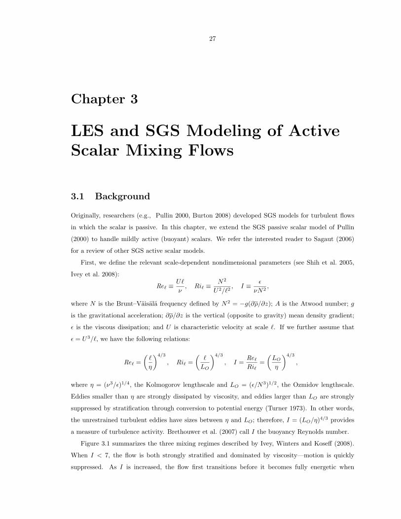
3.4 LES and DNS comparisons of velocity spectra in log–linear coordinates . . . . . . . . 35

3.5 LES and DNS comparisons of the velocity-anisotropy parameter . . . . . . . . . . . . 36

3.6 Normalized scalar flux using passive scalar SGS model . . . . . . . . . . . . . . . . . . 43

3.7 Normalized scalar flux using active scalar SGS model . . . . . . . . . . . . . . . . . . 44

4.1 Schematic of near-wall setup . . . . . . . . . . . . . . . . . . . . . . . . . . . . . . . . 55

4.2 Schematic of attached near-wall counterrotating vortices . . . . . . . . . . . . . . . . . 57

4.3 Code validation with the simulation of Kim, Moin and Moser (1987): mean velocity . 65

4.4 Code validation with the simulation of Kim, Moin and Moser (1987): turbulence statistics 65

4.5 Mean velocity profiles from LES with γIII = 0 . . . . . . . . . . . . . . . . . . . . . . . 67

4.6 Turbulence statistics from LES with γIII = 0 . . . . . . . . . . . . . . . . . . . . . . . 68

4.7 Mean velocity profiles from LES with γIII = 0.45 . . . . . . . . . . . . . . . . . . . . . 69

4.8 Turbulence statistics from LES with γIII = 0.45 . . . . . . . . . . . . . . . . . . . . . . 70

4.9 Subgrid kinetic energy fraction . . . . . . . . . . . . . . . . . . . . . . . . . . . . . . . 70

4.10 P.d.f.s of predicted Karman constant . . . . . . . . . . . . . . . . . . . . . . . . . . . . 71

4.11 Wall model sensitivity to virtual wall location . . . . . . . . . . . . . . . . . . . . . . . 72

4.12 Resolved spectra compared with the model spectrum of Pope (2000) . . . . . . . . . . 72

x

4.13 Effect of grid resolution on LES spectra . . . . . . . . . . . . . . . . . . . . . . . . . . 74

4.14 Streamwise velocity spectra at various wall-normal locations . . . . . . . . . . . . . . 75

4.15 Streamwise, spanwise, and wall-normal velocity spectra at quarter-channel height . . . 76

5.1 Effect of filter size on large-scale–small-scale correlations at Reτ = 2k . . . . . . . . . 81

5.2 Effect of filter size on large-scale–small-scale correlations at Reτ = 200 k . . . . . . . . 82

5.3 Profiles of large-scale–small-scale correlations at Reτ = 2k . . . . . . . . . . . . . . . 83

5.4 Profiles of large-scale–small-scale correlations at Reτ = 200 k . . . . . . . . . . . . . . 83

xi

List of Tables

2.1 DNS parameters for statistically stationary buoyancy-driven turbulence . . . . . . . . 18

4.1 LES parameters and outputs for turbulent channel flow . . . . . . . . . . . . . . . . . 66

5.1 LES parameters for long channel flows . . . . . . . . . . . . . . . . . . . . . . . . . . . 80

1

Chapter 1

Introduction

In the present research, we extend our capability to simulate complex fluid behavior. This research

represents a contribution to the area of computational fluid dynamics, which has and will continue

to have enormous impact on many diverse areas of science and engineering over a large range of

Reynolds numbers, from the galactic scale, through climate modeling, to industrial and engineering

applications.

The ideal is direct numerical simulation (DNS) in which all relevant physical processes are prop-

erly represented and all lengthscales are resolved. For turbulence this will include the Kolmogorov

energy-dissipation scales and the Batchelor scalar-dissipation scales. At the large Reynolds numbers

required for practical engineering applications, full DNS for all but the simplest physics and bound-

ary conditions is unlikely to be practicable for many decades to come. The standard engineering

prediction tool has been Reynolds-averaged modeling (RANS). Whilst RANS will remain useful

for many applications, there is a growing need for a more detailed, DNS-like but computationally

tractable, simulation capability in engineering. Examples include engine, energy, and environmen-

tal applications where physically realistic modeling of turbulent mixing, combustion, and near-wall

flows is required. In particular, the absence of a reliable numerical simulation method at moderate

cost for near-wall flows is perhaps the most severe roadblock to the further expansion of our present

engineering prediction capabilities.

To address this growing need, we develop the multiscale large-eddy simulation (LES) approach in

which conventional LES is enhanced by a physical representation of unresolved subgrid-scale (SGS)

dynamics. While we do not expect to achieve DNS fidelity, we believe that multiscale LES can bring

LES predictions substantially closer to the DNS ideal for many turbulent flows of practical interest,

but at a small fraction of DNS cost. This is the focus of the present work. First, we describe the

LES methodology.

2

1.1 LES

LES, the numerical simulation of fluid flow in which large-scale motion (“large eddy”) is computed

directly while small-scale motion is modeled, shows considerable potential for the underresolved but

accurate simulation of complex turbulent flows. To date, an LES practitioner wishing to simulate

a turbulent flow effectively assumes that the dynamics of large-scale, resolved eddies are dominated

by the flow geometry along with associated large-scale boundary conditions or other turbulence-

generating forcing. Accordingly, it is then thought sufficient to simulate numerically only those

large eddies yet retain the capability to accurately recover at least first- and second-order statistics

(means, correlations, and power spectral densities). The underlying ansatz is that the small scales

are universal and can be parameterized in some way by the local resolved flow properties, with no

explicit dependence on boundary conditions. If these assumptions are valid, successful LES should

require only a computational grid that scales with flow geometry; specifically, the computational

grid should be independent, O(1) or weakly dependent, O(log Re), say, on the Reynolds number

Re. LES promises enormous resource savings when compared to the prohibitively expensive but

accurate DNS, where all scales of motion are computed. Typically, the required number of grid

points for DNS scales as O(Re9/4) (Rogallo and Moin 1984), which measures the size of the largest

eddy relative to the smallest eddy in three dimensions. Further, the need to compute all scales,

and then to perform massive data reduction renders DNS an inefficient and unpractical engineering

design tool.

Also, fundamental questions in LES remain unanswered. For example, it is unclear how the LES

resolved velocity is related to the observed real-world velocity. Pope (2004) provides some insight

into this question. He argued that the relationship is one that is statistical. That is, the statistics of

the observed velocity should only be compared to the model statistics obtained from the combination

of both the LES resolved velocity and the modeled SGS motion. In particular, the statistics of the

LES resolved velocity need not resemble the statistics obtained from the filtered observed velocity.

This also raises the question of the meaning of LES-derived weather predictions at a given space

and time, such as hurricane track predictions. In practice, the LES computation is correlated to

the observed velocity up to a time horizon. For this reason, numerical weather prediction models

are calibrated regularly to incorporate up-to-date observations. Indeed, even DNS, which aims to

resolve all motions, but with finite resolution, is unable to provide accurate pointwise space–time

predictions indefinitely.

Since the early work on LES by Smagorinsky (1963) and Deardorff (1970), LES has met with

a mix of success and challenges. It is fair to say that the outcome of an LES depends largely

on the validity of the assumptions held by our hypothetical LES practitioner. For flows in which

these assumptions apply, typically unbounded flows, such as homogeneous isotropic turbulence (e.g.,

3

Misra and Pullin 1997), shear and wake/jet turbulence, and even the more challenging Richtmyer–

Meshkov instability (e.g., Hill, Pantano and Pullin 2006), LES has performed exceedingly well.

Despite continuing efforts, however (e.g., Cabot and Moin 1999, Voelkl, Pullin and Chan 2000,

Piomelli and Balaras 2002, Wang and Moin 2002, Templeton, Medic and Kalitzin 2005, Piomelli

2008), the LES of wall-bounded flows, while improving, remains a challenging area of research.

One way forward is to augment LES with a physical description of the underlying SGS dynamics

(multiscale LES). However, a detailed accounting of turbulence that contains all orders of statistical

correlations is unnecessary at best and a waste of resources at worst since the main purpose of SGS

modeling is to capture the average effects (low-order statistics) of the underresolved turbulence.

Presently, this is accomplished via a simple vortex-based model of the SGS dynamics.

1.2 Vortex-Based SGS Model

Despite the complex nature of turbulence, simple vortex-based models have been successfully used

to predict many statistical properties of turbulence (Lundgren 1982, Perry and Chong 1982, Pullin

and Saffman 1994, Pullin and Lundgren 2001, O’Gorman and Pullin 2003). Presently, we focus on

its use as a basis for SGS modeling in LES.

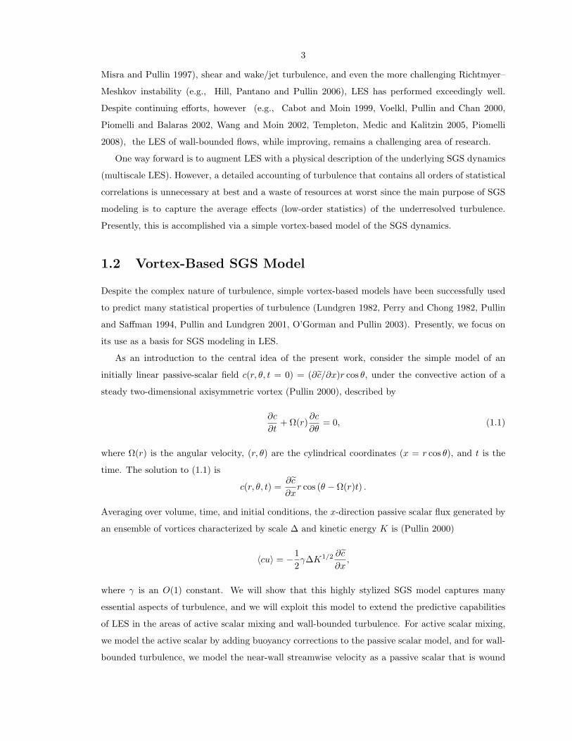
As an introduction to the central idea of the present work, consider the simple model of an

initially linear passive-scalar field c(r, θ, t = 0) = (∂c/∂x)r cos θ, under the convective action of a

steady two-dimensional axisymmetric vortex (Pullin 2000), described by

∂c

∂t+ Ω(r)

∂c

∂θ= 0, (1.1)

where Ω(r) is the angular velocity, (r, θ) are the cylindrical coordinates (x = r cos θ), and t is the

time. The solution to (1.1) is

c(r, θ, t) =∂c

∂xr cos (θ − Ω(r)t) .

Averaging over volume, time, and initial conditions, the x-direction passive scalar flux generated by

an ensemble of vortices characterized by scale ∆ and kinetic energy K is (Pullin 2000)

〈cu〉 = −12γ∆K1/2 ∂c

∂x,

where γ is an O(1) constant. We will show that this highly stylized SGS model captures many

essential aspects of turbulence, and we will exploit this model to extend the predictive capabilities

of LES in the areas of active scalar mixing and wall-bounded turbulence. For active scalar mixing,

we model the active scalar by adding buoyancy corrections to the passive scalar model, and for wall-

bounded turbulence, we model the near-wall streamwise velocity as a passive scalar that is wound

4

by attached streamwise vortices.

1.3 Plan of Thesis

The two areas of the present research are active scalar mixing and wall-bounded turbulence. To

better understand active scalar mixing, we propose a novel method to perform DNS of statistically

stationary buoyancy-driven turbulence in chapter 2. In chapter 3, we develop an SGS model for

active scalar mixing based on the vortex model given in § 1.2. We then shift our focus to developing

a wall model for LES in chapter 4, again using ideas from § 1.2. Finally, we provide an application

of the new wall model in chapter 5 before concluding in chapter 6. Owing to the different areas of

specialization, each chapter will have its own set of notations.

5

Chapter 2

DNS of Statistically StationaryBuoyancy-Driven Turbulence

2.1 Background

The buoyancy-driven turbulent mixing of variable-density fluids arises in many applications, ranging

from the naturally occurring exploding supernovae to the man-made inertial confinement fusion, and

from the weighty subject of environmental pollution to the whimsical emptying of an inverted glass of

water (Sandoval 1995, Cook and Dimotakis 2001, Dimotakis 2005). To better understand and predict

these flows, researchers have proposed various ways to capture the essential physics of these flows

in simple models that lend themselves to academic investigation through laboratory experiments,

numerical simulations, and theoretical development.

In the spirit of such efforts, we propose a new model for the simulation of statistically stationary

buoyancy-driven turbulent mixing of a variable-density fluid by employing a fringe region (Bertolotti,

Herbert and Spalart 1992, Nordstrom, Nordin and Henningson 1999), which sustains an unstable

density gradient within a triply periodic domain, in the presence of gravity. Following Sandoval

(1995), we consider an incompressible binary fluid mixture comprised of fluids with microscopic

densities ρ1 and ρ2, with the convention ρ2 > ρ1. Presently, we are interested in moderately high

density ratios R (≡ ρ2/ρ1), namely R = 3 and 7, a regime in which the Boussinesq assumption,

formally R = 1, is no longer valid. The present model draws on many loosely related ideas from the

literature; we will highlight some important similarities and differences in the following.

Overholt and Pope (1996), Yeung, Donzis and Sreenivasan (2005) simulated, in a triply peri-

odic domain, the mixing of a passive scalar by forced isotropic–homogeneous turbulence embedded

in background mean scalar gradient. Passive scalar fluctuations are continually produced by the

background mean scalar gradient, but are kept in balance by diffusive dissipation, resulting in a

statistically stationary flow. While, like Overholt and Pope (1996), our present model can also be

viewed as a statistically stationary scalar-mixing flow in a background scalar gradient, there are two

6

important distinctions. First, the present model considers an active scalar, the mass fraction (alge-

braically related to the density), whose spatial variation is the source of buoyant potential energy

that solely supplies the turbulent kinetic energy; in the model of Overholt and Pope (1996), the

velocity field is forced externally. Second, the active scalar precludes a straightforward extension of

the Overholt and Pope (1996) model for sustaining a passive scalar gradient because the resulting

equations for the active scalar fluctuations can no longer be simulated in a triply periodic domain.

We adapt the fringe-region technique (Bertolotti, Herbert and Spalart 1992) to our problem to

overcome this difficulty.

Employing the Boussinesq assumption, Batchelor, Canuto and Chasnov (1992) studied the buo-

yancy-driven turbulent mixing of an active scalar in a triply periodic domain. A feature absent

in Boussinesq flows is baroclinic vorticity, generated by misalignments between pressure and den-

sity gradients. Later, Sandoval (1995) and Livescu and Ristorcelli (2007, 2008) performed similar

computations, generalizing to higher density ratios, and without using the Boussinesq assumption.

All of these flows were initialized with blobs of unmixed fluid and allowed to decay as the initial

potential energy is converted to kinetic energy, which drives the turbulent mixing, before it is fi-

nally dissipated by diffusion. Like Sandoval (1995), we presently compute the turbulent mixing of

a moderately high-R incompressible binary fluid mixture within a triply periodic domain, but we

additionally use a fringe region to sustain an unstable density gradient (heavy fluid on top of light

fluid) to produce a statistically stationary flow.

Perhaps the most widely used model to study buoyancy-driven turbulent mixing is the Rayleigh–

Taylor instability (e.g., Cook and Dimotakis 2001, Cook, Cabot and Miller 2004, Cabot and Cook

2006, Mueschke and Schilling 2009), where an initial perturbed interface separating unmixed heavy

fluid on top of light fluid is accelerated toward the light fluid, resulting in a growing turbulent mixing

layer. Rayleigh–Taylor instability is a statistically evolving flow, requiring expensive computational

resources (e.g., Cabot and Cook 2006) to capture late-time asymptotic self-similar statistics. Our

present simulations can perhaps be viewed as a model for the late-time Rayleigh–Taylor instability

deep within the interior of the turbulent mixing zone, where the slowly evolving fine-scale turbu-

lence is informed of the far-field boundary conditions only through the unstable density gradient.

The analogy is incomplete, however, as a statistically evolving flow is fundamentally different to a

statistically stationary flow. Two other flows that are related in this same way are forced isotropic–

homogeneous turbulence and decaying isotropic–homogeneous turbulence.

A somewhat related flow is the closed-vessel experiment of Krawczynski et al. (2006), where

passive scalar mixing is achieved by a continual injection of unmixed fluids from a series of impinging

jets, resulting in a statistically stationary homogeneous isotropic turbulent flow. In the present

simulations, the role of the jets is played by the fringe region, where unmixed fluids are continually

introduced into the domain. Again, we consider a dynamically active scalar, and unlike the jets in

7

the experiment, the fringe region is not a source of momentum.

The plan of the chapter is as follows. The governing equations with source terms and the variable-

density incompressible fluid model is introduced in § 2.2.1. We then determine the restrictions on

the source terms when solving these equations in a triply periodic domain (§ 2.2.2). In § 2.2.3, we

introduce our adaptation of the fringe-region technique, and then prescribe a condition on the exter-

nal pressure gradient in § 2.2.4. A new method for solving the governing equations that guarantees

discrete mass conservation, regardless of iteration errors, is described in § 2.3.1. The numerical

discretization is detailed in § 2.3.2. We present results, including profiles of integral quantities, com-

parisons of present spectra with the Rayleigh–Taylor instability spectra of Cabot and Cook (2006)

and mole fraction probability density functions in § 2.4.

2.2 Problem Description

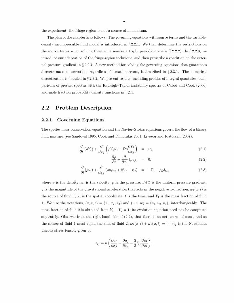
2.2.1 Governing Equations

The species mass conservation equation and the Navier–Stokes equations govern the flow of a binary

fluid mixture (see Sandoval 1995, Cook and Dimotakis 2001, Livescu and Ristorcelli 2007):

∂

∂t(ρY1) +

∂

∂xj

(ρY1uj −Dρ

∂Y1

∂xj

)= ω1, (2.1)

∂ρ

∂t+

∂

∂xj(ρuj) = 0, (2.2)

∂

∂t(ρui) +

∂

∂xj(ρuiuj + pδij − τij) = −Γi − ρgδi3, (2.3)

where ρ is the density; ui is the velocity; p is the pressure; Γi(t) is the uniform pressure gradient;

g is the magnitude of the gravitational acceleration that acts in the negative z-direction; ω1(x, t) is

the source of fluid 1; xi is the spatial coordinate; t is the time; and Y1 is the mass fraction of fluid

1. We use the notations, (x, y, z) = (x1, x2, x3) and (u, v, w) = (u1, u2, u3), interchangeably. The

mass fraction of fluid 2 is obtained from Y1 + Y2 = 1; its evolution equation need not be computed

separately. Observe, from the right-hand side of (2.2), that there is no net source of mass, and so

the source of fluid 1 must equal the sink of fluid 2, ω1(x, t) + ω2(x, t) = 0. τij is the Newtonian

viscous stress tensor, given by

τij = µ

(∂ui

∂xj+∂uj

∂xi− 2

3δij∂uk

∂xk

).

8

The nondimensional parameters that characterize the present flow are the Reynolds, Schmidt and

Froude numbers, defined as

Re ≡ ρ0U`/µ, Sc ≡ µ/(ρ0D), Fr2 ≡ U2/(g`),

where ρ0 is the density scale; U is the velocity scale; ` is the lengthscale; µ = µ1 = µ2 is the constant

matched dynamic viscosity for both fluids; and D is the Fickian diffusion coefficient.

Density variation arises purely from variation in the local fluid composition. The relevant equa-

tion of state is then (Sandoval 1995)

1ρ(x, t)

=Y1(x, t)ρ1

+Y2(x, t)ρ2

= Y1(x, t)(

1ρ1− 1ρ2

)+

1ρ2, (2.4)

where ρ1 and ρ2 are the constant microscopic densities of their respective fluids. We fix the density

scale ρ0 = (ρ1 + ρ2)/2 so that

ρ1

ρ0= 1−A and

ρ2

ρ0= 1 +A, where A ≡ ρ2 − ρ1

ρ2 + ρ1=R− 1R+ 1

> 0, (2.5)

the Atwood number. Next, fix the velocity scale,

U = (Ag`)1/2 ⇒ Re = ρ0(Ag`)1/2`/µ, Fr2 = A,

making Re, Sc and A the three independent parameters for this flow. Presently, Sc = 1; we then

perform a parametric study in the (Re, A) space.

We eliminate Y1 by combining (2.1) and (2.4), and then using (2.2) to get

∂uj

∂xj= −D ∂

∂xj

(1ρ

∂ρ

∂xj

)− ωs, where ωs ≡

(1ρ2− 1ρ1

)ω1, (2.6)

in contrast to constant density flows, where ∂uj/∂xj = 0. We combine (2.6) and (2.2) to write

∂s

∂t+ uj

∂s

∂xj= D ∂

2s

∂x2j

+ ωs, (2.7)

where s ≡ log(ρ/ρ0). We will use (2.7) as an alternative evolution equation for ρ.

2.2.2 Consequences of Periodicity

We wish to compute a nontrivial solution to the governing equations in a periodic domain. Given this

constraint, we will now determine how to obtain a flow that is statistically stationary by choosing

ω1 in (2.1) or equivalently ωs in (2.6). Denote the volume average by ( ), then periodicity implies

9

∂( )/∂xj = 0. From (2.1) and (2.2),

∂

∂tρY1 = ω1,

∂ρ

∂t= 0. (2.8)

Without loss of generality, set ρ = ρ0. We rearrange (2.4) and (2.5), then average, to get

ρY1 = (1− ρ/ρ2) /(1/ρ1 − 1/ρ2) = ρ1/2 = ρ0(1−A)/2.

Likewise, ρY2 = ρ0(1 +A)/2. Since ρY1 is a constant, (2.8) necessarily implies that ω1 = ωs = 0 at

every instant of time.

Decomposing ρ = ρ+ ρ′, we can obtain the evolution equation for ρ′2 from (2.2):

∂ρ′2

∂t+∂(ujρ

′2)∂xj

+(ρ2 − ρ2

) ∂uj

∂xj= 0. (2.9)

Use (2.6) to calculate

ρ2 ∂uj

∂xj= −D

[∂2

∂x2j

(12ρ2

)− 2

(∂ρ

∂xj

)2]− ρ2ωs,

which we then combine with the volume average of (2.9) to obtain the equation governing the density

fluctuation variance:∂ρ′2

∂t= −2D

(∂ρ′

∂xj

)2

+ ρ2ωs. (2.10)

Denote the long-time average by 〈 〉∞, then 〈∂( )/∂t〉∞ = 0 for any statistically stationary quantity.

Time averaging (2.10),

2D⟨(∂ρ′/∂xj)

2⟩∞

=⟨ρ2ωs

⟩∞> 0. (2.11)

We choose ωs(x, t) = 0 except in a region called the fringe. Then (2.11) says that, over time, the

source of unmixed fluids, introduced in the fringe, necessarily balances the mixing occurring outside

the fringe, resulting in a statistically stationary flow.

2.2.3 Fringe-Region Forcing

A source of unmixed fluids in unstable configuration (heavy fluid on top of light fluid) is required for

buoyancy forces to drive the turbulent mixing process. In Rayleigh–Taylor turbulence, the infinite

reservoirs of unmixed fluid supply the mixing zone, but the flow is not stationary owing to the

growing height of the mixing zone. The kind of stationary flow that we envision presently has

similarities with the partially stirred reactor of Krawczynski et al. (2006), which was used to study

passive scalar mixing by jet-driven turbulence in a closed vessel. In our case, the scalar is active and

10

the turbulence is driven by buoyancy (not momentum).

Our goal is to simulate a turbulent mixing flow in a triply periodic domain. In the absence of

any forcing, the flow decays, which is the flow computed by Livescu and Ristorcelli (2007). The

present approach is to approximate the mixing chamber by using the fringe-region technique (e.g.,

Bertolotti, Herbert and Spalart 1992, Nordstrom, Nordin and Henningson 1999). A natural choice

is to apply the technique directly to the source term ω1 in (2.1):

ω1(x, t) = Λ1λ1(x)ρ1Y2(x, t)− Λ2λ2(x)ρ2Y1(x, t), (2.12a)

or equivalently, using (2.4) and (2.6),

ωs(x, t) = Λ1λ1(x)(ρ1/ρ(x, t)− 1) + Λ2λ2(x)(ρ2/ρ(x, t)− 1), (2.12b)

where 0 ≤ λ1, λ2 ≤ 1 are the smooth fringe indicator functions (1 inside the fringe region, 0 outside

the fringe region) corresponding to the respective fluid sources. Momentarily setting (λ1, λ2) = (1, 0)

in (2.12a), observe that the rate at which the light fluid is introduced in the flow is proportional

to its microscopic density ρ1 and its mass fraction deficit Y2 = 1 − Y1. A similar statement can be

made for the heavy fluid source. The indicator functions are defined by

λ1(x) = ξ1(x, y) [Π(z; 0, 0 + Lf ) + Π(z;Lz, Lz + Lf )] , (2.13a)

λ2(x) = ξ2(x, y) [Π(z; 0− Lf , 0) + Π(z;Lz − Lf , Lz)] , (2.13b)

where Lz is the height of the periodic domain, shown in figure 2.1(a); Lf/` = 2π/10, the height of

the fringe region; 0 ≤ ξ1, ξ2 ≤ 1 are planar indicator functions to be defined; and Π is a top-hat

function constructed from smooth step functions S (see figure 2.1(b))

Π(z; zstart, zend) = S

(z − zstart

∆rise+

12

)− S

(z − zend

∆fall+

12

), (2.14a)

S(z) =

0, z ≤ 0,

1/[1 + exp

(1

z−1 + 1z

)], 0 < z < 1,

1, z ≥ 1.

(2.14b)

We choose transition widths ∆rise = ∆fall = 6∆z, where ∆z is the computational grid height. λ1(x)

and λ2(x) in (2.13) are chosen so that heavy fluid is introduced at the top of the flow domain and

light fluid is introduced at the bottom of the domain. We use Π twice in each of (2.13) to preserve

vertical periodicity.

The planar indicator functions have zero mean: 〈ξ1(x, y)〉 = 〈ξ2(x, y)〉 = 0, where 〈 〉 denotes the

11

(a)

x

y

z

g

Lz

Ly

Lx

Lf

Lf

ρ1

ρ2

(b)

Π(z)

z

Δrise

Δfall

1

zstart

zend

(c)

Figure 2.1. (a) Triply periodic flow domain showing the shaded fringe regions that supply theflow with unmixed fluids, heavy above light (ρ2 > ρ1). (b) Features of the smooth function Π(z),(2.14a), used to locate the fringe region. (c) Horizontal slice of the planar indicator function ξ1(x, y),constructed from applying the Gaussian spectral filter to a physical i.i.d. random field of N(0, 1).The filter is centered on wavenumber k0` corresponding to wavelength λ0/` = 2π/16 and the boxshown has dimensions 2π`× 2π`.

12

xy-plane average. They are constructed in a manner similar to the construction of the perturbation

field used by Cook, Cabot and Miller (2004). Briefly, independent and identically distributed (i.i.d.)

normal random variables with zero mean and unit variance, N(0, 1), are assigned to each (x, y) grid

point. We transform this field to Fourier space and apply a Gaussian filter centered on wavenumber

k0` = 16 with standard deviation σk` = 4. The resulting field is transformed back to physical space

with value ζ(x, y) and steepened with the function

ξ1(x, y) = 1/2 + arctan[πζ(x, y)/(3σζ)]/π,

where σζ is the standard deviation of ζ. A contour plot of ξ1 is shown in figure 2.1(c).

Omitting convection and diffusion in (2.7), then substituting (2.12b), we obtain the simple balance

between the source term and the unsteady term in the fringe:

∂ρ

∂t=

Λ1(ρ1 − ρ) if (λ1, λ2) = (1, 0),

Λ2(ρ2 − ρ) if (λ1, λ2) = (0, 1).(2.15)

Observe that ωs is designed to force ρ(x, t) following a fluid particle to track ρ1 (or ρ2) at the rate

Λ1 (or Λ2). The fringe region parameters, Λ1 and Λ2, are similar to the Damkohler number used

in chemical reactions—it measures the strength of the source of unmixed fluids, introduced in the

fringe, relative to the flow. The parameters, Λ1 and Λ2, can also be interpreted as inverse time

constants of first-order systems, clearly seen in structure of (2.15). They are not independent; recall

from § 2.2.2 the constraint ω1 = 0, implying that

Λ1λ1(x, t)(ρ1/ρ− 1) + Λ2λ2(x, t)(ρ2/ρ− 1) = 0.

It remains to fix the upper limit:

Λ = maxΛ1,Λ2.

We use an order-of-magnitude argument to choose Λ. Since the fringe introduces unmixed fluids

with densities ρ1 and ρ2 in a layer of width Lf subjected to gravity g, its characteristic velocity

scale is Uf = (AgLf )1/2. The time it takes for a fluid particle to transit through fringe is Tf =

Lf/Uf = (Lf/Ag)1/2. We then choose Λ(`/Ag)1/2 = 10, which is much larger than the transit rate,

(`/Ag)1/2/Tf = (`/Lf )1/2 = (10/2π)1/2 ≈ 1.26, a source rate high enough, relative to the flow, in

order for ρ(x, t) to take on the desired values ρ1 or ρ2.

13

2.2.4 Mean Pressure Gradient

A model is required for Γi(t), the externally imposed spatially uniform pressure gradient. In

Rayleigh–Taylor turbulence, the far-field quiescent boundary conditions determines Γi felt in the

turbulent mixing zone. In a triply periodic domain where such far-field boundary conditions cannot

be directly imposed, we model Γi by requiring that 〈∂ui/∂t〉z=Lz/2 = 0, where 〈 〉z=Lz/2 denotes

the xy-plane average taken at the z = Lz/2 plane (midplane). As noted by Livescu and Ristor-

celli (2007), 〈∂ui/∂t〉z=Lz/2 ≈ 0 in the turbulent mixing zone, who considered a similar model by

choosing ∂ui/∂t = 0. For definiteness, we choose 〈ui〉z=Lz/2 = 0.

Alternatively, Γi can also be determined from the volume average of (2.3),

∂

∂tρui = −Γi(t)− ρgδi3.

Upon taking the long-time average, the ∂/∂t term vanishes, and we obtain 〈Γi〉∞ = −ρgδi3. That

is, over time, Γi(t) fluctuates about its theoretical steady state. We use this result to check the

internal consistency of our code.

2.3 Solution Method

2.3.1 Alternative Lagrange Multiplier to Pressure

In incompressible flows, a constraint on the velocity divergence has to be satisfied at all times. For

variable density flows, the constraint is (2.6), while for constant density flows, the constraint is

∂uj/∂xj = 0. This is enforced by treating p as a Lagrange multiplier. The elliptic equation for

p is obtained by taking the divergence of (2.3), then enforcing the constraint (2.6). In constant

density flows, this results in a constant-coefficient Poisson equation for p, which is readily solved.

The nonconstant 1/ρ factor in variable density flows presents an additional complication.

This issue appears in a variety of forms in the literature and cannot be circumvented. Sandoval

(1995) and Cook and Dimotakis (2001), for example, take the divergence of (2.3), resulting in a

constant-coefficient Poisson equation for p, but use what amounts to a lower-order extrapolation for

∂ui/∂t, reducing the overall accuracy of the temporal discretization. Consequently, mass conserva-

tion in the form of (2.6) is never satisfied instantaneously. The advantage to their approach is that

no iterations are required. Another approach to this issue is proposed by Livescu and Ristorcelli

(2007), who derive an exact nonlinear equation for p (equation A15 in that paper) that requires an

iterative solution method but eliminates temporal discretization errors. However, it remains that

(2.6) cannot be discretely satisfied owing to the inevitable finite spatial resolution, even if infinite

iterations were possible.

14

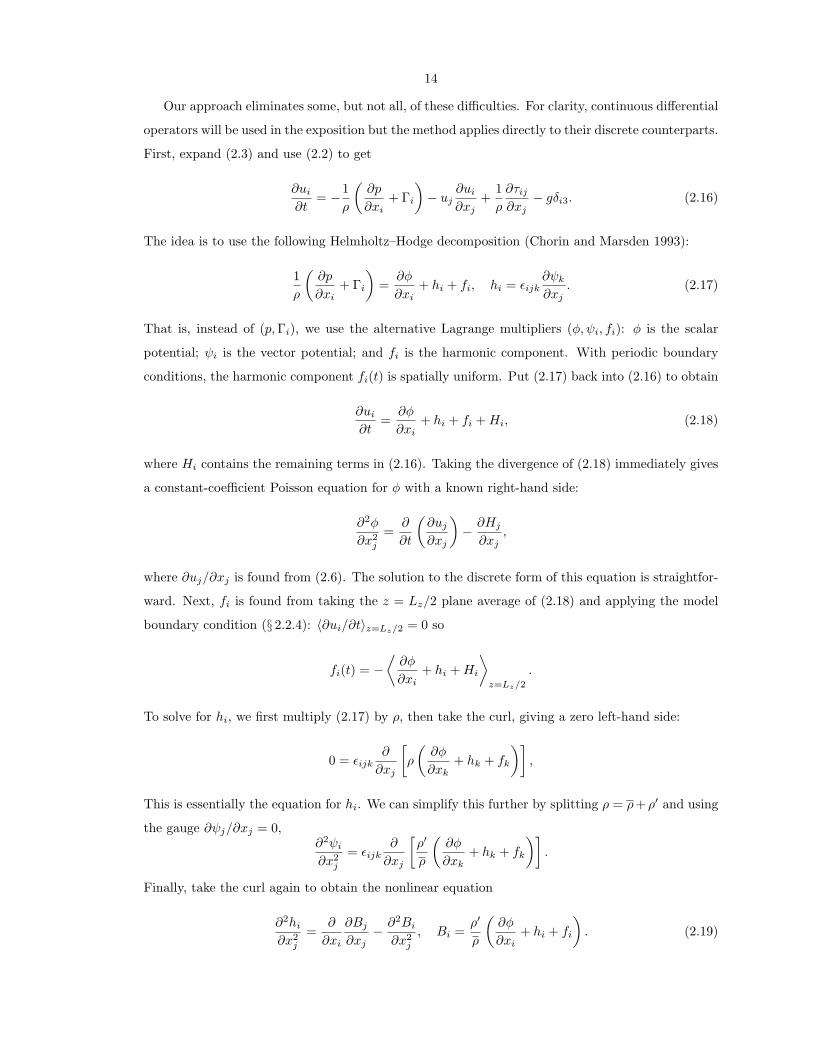
Our approach eliminates some, but not all, of these difficulties. For clarity, continuous differential

operators will be used in the exposition but the method applies directly to their discrete counterparts.

First, expand (2.3) and use (2.2) to get

∂ui

∂t= −1

ρ

(∂p

∂xi+ Γi

)− uj

∂ui

∂xj+

1ρ

∂τij∂xj

− gδi3. (2.16)

The idea is to use the following Helmholtz–Hodge decomposition (Chorin and Marsden 1993):

1ρ

(∂p

∂xi+ Γi

)=

∂φ

∂xi+ hi + fi, hi = εijk

∂ψk

∂xj. (2.17)

That is, instead of (p,Γi), we use the alternative Lagrange multipliers (φ, ψi, fi): φ is the scalar

potential; ψi is the vector potential; and fi is the harmonic component. With periodic boundary

conditions, the harmonic component fi(t) is spatially uniform. Put (2.17) back into (2.16) to obtain

∂ui

∂t=

∂φ

∂xi+ hi + fi +Hi, (2.18)

where Hi contains the remaining terms in (2.16). Taking the divergence of (2.18) immediately gives

a constant-coefficient Poisson equation for φ with a known right-hand side:

∂2φ

∂x2j

=∂

∂t

(∂uj

∂xj

)− ∂Hj

∂xj,

where ∂uj/∂xj is found from (2.6). The solution to the discrete form of this equation is straightfor-

ward. Next, fi is found from taking the z = Lz/2 plane average of (2.18) and applying the model

boundary condition (§ 2.2.4): 〈∂ui/∂t〉z=Lz/2 = 0 so

fi(t) = −⟨∂φ

∂xi+ hi +Hi

⟩z=Lz/2

.

To solve for hi, we first multiply (2.17) by ρ, then take the curl, giving a zero left-hand side:

0 = εijk∂

∂xj

[ρ

(∂φ

∂xk+ hk + fk

)],

This is essentially the equation for hi. We can simplify this further by splitting ρ = ρ+ ρ′ and using

the gauge ∂ψj/∂xj = 0,∂2ψi

∂x2j

= εijk∂

∂xj

[ρ′

ρ

(∂φ

∂xk+ hk + fk

)].

Finally, take the curl again to obtain the nonlinear equation

∂2hi

∂x2j

=∂

∂xi

∂Bj

∂xj− ∂2Bi

∂x2j

, Bi =ρ′

ρ

(∂φ

∂xi+ hi + fi

). (2.19)

15

We solve this by iterating: use the current h(n)i in the right-hand side B(n+1)

i of the Poisson equation

for the next h(n+1)i . If the density is constant, ρ′ = 0 ⇒ Bi = 0 ⇒ hi = 0 to recover (p,Γi) = (φ, fi),

verifiable from (2.19) and (2.17).

Using (2.17) allows the exact satisfaction of mass conservation (2.1) at every time instant and up

to the machine precision of the spatial discretization, regardless of iteration errors in (2.19). This is

because the part of the Lagrange multiplier (1/ρ)(∂p/∂xi) that plays the role of mass conservation

is completely encapsulated by its curl-free component ∂φ/∂xi. All errors from this method are

isolated to iteration residuals in hi. In the vorticity equation, its curl, εijk∂hk/∂xj , is the baroclinic

source of vorticity. In physical terms, the present approach eliminates mass conservation errors but

incurs errors on baroclinic vorticity. However, the vorticity equation is always subject to temporal

discretization errors. A similar approach for the zero-divergence incompressible equations is taken

by Chang, Giraldo and Perot (2002). Presently we control this error by iterating until ||h(n+1)i −

h(n)i ||/||h(n)

i || < 10−2, where || || denotes the L2-norm. In practise, this takes 1–2 iterations.

Since p and Γi have been replaced by φ, ψi, and fi, they are not required for the time integration

of the governing equations. If required for diagnostics, they are readily calculated from

∂2p

∂x2j

=∂

∂xj

[ρ

(∂φ

∂xj+ hj + fj

)], Γi(t) =

[ρ

(∂φ

∂xi+ hi + fi

)].

We remark that the satisfaction of discrete mass conservation is only one of many ways to

assess the “goodness” of a solution. However, anecdotal evidence in the literature suggests that

discrete mass conservation is important for numerical stability. Sandoval (1995), for example, reports

numerical instability when the density ratio is large. Using the present discretization, no such

numerical instability was found, even when R = 7. A study exploring the direct link between

discrete mass conservation and numerical stability is beyond the scope of this work.

2.3.2 Numerical Discretization

The governing equations, in the form (2.6), (2.7), and (2.16), are discretized using the low-storage

semi-implicit Runge-Kutta method of Spalart, Moser and Rogers (1991). Briefly, the method consists

of three sequential substeps of the following form:

s(n+1) − s(n)

∆t= γH(n)

s + ζH(n−1)s + αD ∂2

∂x2j

s(n) + βD ∂2

∂x2j

s(n+1), (2.20a)

u(n+1)i − u

(n)i

∆t= γH

(n)i + ζH

(n−1)i + α

µ

ρ0

∂2

∂x2j

u(n)i + β

µ

ρ0

∂2

∂x2j

u(n+1)i

− (α+ β)ρ(∗)

(∂p

∂xi+ Γi

), (2.20b)

∂

∂xju

(n+1)j = −D ∂2

∂xjs(n+1) − ω(n+1)

s , (2.20c)

16

where

Hs = −uj∂s

∂xj+ ωs,

Hi = −uj∂ui

∂xj+µ

ρ0

[(ρ0

ρ− 1)∂2ui

∂x2j

+ρ0

ρ

13∂

∂xi

∂uj

∂xj

]− gδi3,

ρ ≡ ρ0 exp(s); (α + β)/ρ(∗) ≡ α/ρ(n) + β/ρ(n+1); and ωs is given by (2.12b). The values for α, β,

γ, and ζ, different for each substep, are given in Spalart, Moser and Rogers (1991). For stability,

we have chosen to split the viscous operator into the linear component, which we treat implicitly,

and the nonlinear component, which we treat explicitly. Discretizing s, ∈ (∞,∞), rather than ρ

ensures that ρ > 0, but then, ρ = ρ0 can no longer be maintained discretely; we presently control this

numerical drift with a small proportional control added to Λ1 and Λ2. The Courant–Friedrichs–Levy

condition is dynamically adjusted so that

∆t maxi=1,2,3

|ui|/∆i = 0.7,

where ∆i ≡ Li/Ni. Presently, ∆ ≡ ∆1 = ∆2 = ∆3 everywhere.

The spatial discretization of (2.20) employs the Fourier pseudospectral method (e.g., Canuto

et al. 1987), where the products and nonlinear terms in Hi and Hs are computed in physical space,

then transformed to spectral space for the 2/3-rule dealiasing. The maximum dealiased wavenumber

is then (2/3)(π/∆), where ∆ is the grid size. The 2/3-rule eliminates all aliasing errors arising from

double products, but some higher-order aliasing from quotients and exponentials remains.

The steps for solving the system (2.20) are as follows: First, solve (2.20 a), and then solve (2.20 b),

choosing the Lagrange multipliers (φ, ψi, fi), where

1ρ(∗)

(∂p

∂xi+ Γi

)≡ ∂φ

∂xi+ εijk

∂ψk

∂xj+ fi,

so that (2.20 c) is discretely satisfied and that 〈un+1i 〉z=Lz/2 = 0. The latter step of determining the

Lagrange multipliers is described using continuous operators in § 2.3.1.

2.3.3 Code Validation

As validation of our code, we reproduce the case 3Base of Livescu and Ristorcelli (2007) from three

independent but statistically identical initial conditions (see figure 2.2). This is readily achieved by

setting ωs = 0 in (2.6) and (2.7) and initializing the flow as random blobs of pure fluids in a cube of

size 2π`, a procedure documented in Livescu and Ristorcelli (2007). There is some statistical spread

in the present initial conditions: the initial integral lengthscale Lρ/` = 0.3542–0.3550, and the initial

density fluctuations ρrms/ρ = 0.2248–0.2252. Livescu and Ristorcelli (2007) reported these numbers

17

0.0

0.2

0.4

0.6

0 5 10 15 20

t(Ag/)1/2

ρuiui

2ρ(Ag)

(a)

0 2 4 6 8

t(Ag/)1/2

ρrms/ρ

(b)

Figure 2.2. The present code shows fair agreement when validated against a simulation performedby Livescu and Ristorcelli (2007) ( ). Three independent but statistically identical simulations areshown ( ).

as 0.3525 and 0.22 respectively.

2.4 Results and Discussion

The simulation parameters are given in table 2.1. In each case, the horizontal cross section is a

square, Lx = Ly. To assess sensitivities to the choice of computational domain we perform the

set of cases A, B, and C, which have identical Re and A, but different computational domains:

case A in a cube domain Lz = Lx, case B in a short domain Lz = Lx/2, and case C is a tall

domain Lz = 2Lx. Cases C, D, E, and F share the same tall domains, but have the four different

permutations of A = 1/2, 3/4 and Re = (256/2π)3/2, (384/2π)3/2 = 260, 478. The grid

Reynolds number Re∆ ≡ ρ0(Ag∆)1/2∆/µ = Re(∆/`)3/2 is set to unity; the grid is equidimensional,

∆ = Lx/Nx = Ly/Ny = Lz/Nz. Simulations were advanced until volume-averaged statistics appear

to reach a statistically stationary state at t = tstart. Then all statistics are averaged over Te eddy-

turnover times, defined as

Te ≡ (tend − tstart)(u′iu′i/3)1/2/Lx,

listed in table 2.1. Unless stated otherwise, we will remove time dependence from all statistics to

imply time averaging, avoiding cumbersome notation.

Visualizations of the heavy fluid mole fraction are shown in figure 2.3.

18

Table 2.1. DNS parameters for statistically stationary buoyancy-driven turbulence.

Key Case Re Re∆ Sc A R Lx/` Ly/` Lz/` Lf/` Nx Ny Nz Te

A 260 1 1 1/2 3 2π 2π 2π 2π/10 256 256 256 5.6B 260 1 1 1/2 3 4π 4π 2π 2π/10 512 512 256 3.2C 260 1 1 1/2 3 2π 2π 4π 2π/10 256 256 512 5.3D 260 1 1 3/4 7 2π 2π 4π 2π/10 256 256 512 8.5E 478 1 1 1/2 3 2π 2π 4π 2π/10 384 384 768 5.3F 478 1 1 3/4 7 2π 2π 4π 2π/10 384 384 768 4.0

(a) (b)

(c) (d) (e) (f )

Figure 2.3. Representative xz-plane visualizations of X2, defined by (2.23). Gravity points down-ward. The shades vary from light to dark as X2 vary from 0 to 1. See table 2.1 for simulationparameters. (a) case A, (b) case B, (c) case C, (d) case D, (e) case E, and (f ) case F.

19

0

1

2

3

4

0 0.5 1

z

π

(a)

0 0.5 1

(b)

−1 0 1

(c)

0

1

2

0 0.5 1

lρ/Lx

z

π

(d)

0 0.5 1

〈X2〉

(e)

−1 0 1

σ(z, Lz/2)

(f )

Figure 2.4. Profiles of the integral quantities lρ defined by (2.21),X2 defined by (2.23), and σ(z, Lz/2)defined by (2.24) (see table 2.1 for key). Horizontal lines indicate fringe-region boundaries.

20

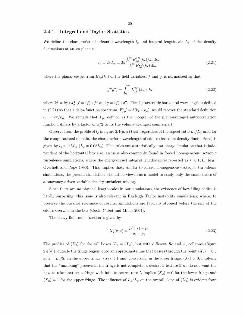
2.4.1 Integral and Taylor Statistics

We define the characteristic horizontal wavelength lρ and integral lengthscale Lρ of the density

fluctuations at an xy-plane as

lρ ≡ 2πLρ ≡ 2π

∫∞0E2D

ρρ (kr)/kr dkr∫∞0E2D

ρρ (kr) dkr

, (2.21)

where the planar cospectrum Efg(kr) of the field variables, f and g, is normalized so that

〈f ′′g′′〉 =∫ ∞

0

E2Dfg (kr) dkr, (2.22)

where k2r = k2

x+k2y, f = 〈f〉+f ′′ and g = 〈f〉+g′′. The characteristic horizontal wavelength is defined

in (2.21) so that a delta-function spectrum, E2Dρρ = δ(kr−kρ), would recover the standard definition

lρ = 2π/kρ. We remark that Lρ, defined as the integral of the plane-averaged autocorrelation

function, differs by a factor of π/2 to its the volume-averaged counterpart.

Observe from the profile of lρ in figure 2.4(a, d) that, regardless of the aspect ratio Lz/Lx used for

the computational domain, the characteristic wavelength of eddies (based on density fluctuations) is

given by lρ ≈ 0.5Lx (Lρ ≈ 0.08Lx). This rules out a statistically stationary simulation that is inde-

pendent of the horizontal box size, an issue also commonly found in forced homogeneous–isotropic

turbulence simulations, where the energy-based integral lengthscale is reported as ≈ 0.15Lx (e.g.,

Overholt and Pope 1996). This implies that, similar to forced homogeneous–isotropic turbulence

simulations, the present simulations should be viewed as a model to study only the small scales of

a buoyancy-driven variable-density turbulent mixing.

Since there are no physical lengthscales in our simulations, the existence of box-filling eddies is

hardly surprising; this issue is also relevant in Rayleigh–Taylor instability simulations, where, to

preserve the physical relevance of results, simulations are typically stopped before the size of the

eddies overwhelm the box (Cook, Cabot and Miller 2004).

The heavy-fluid mole fraction is given by

X2(x, t) =ρ(x, t)− ρ1

ρ2 − ρ1. (2.23)

The profiles of 〈X2〉 for the tall boxes (Lz = 2Lx), but with different Re and A, collapses (figure

2.4(b)), outside the fringe region, onto an approximate line that passes through the point 〈X2〉 = 0.5

at z = Lz/2. In the upper fringe, 〈X2〉 < 1 and, conversely, in the lower fringe, 〈X2〉 > 0, implying

that the “unmixing” process in the fringe is not complete, a desirable feature if we do not want the

flow to relaminarize; a fringe with infinite source rate Λ implies 〈X2〉 = 0 for the lower fringe and

〈X2〉 = 1 for the upper fringe. The influence of Lz/Lx on the overall slope of 〈X2〉 is evident from

21

0

1

2

3

4

0 150 300

z

π

(a)

0 75 150

(b)

0.0 0.2 0.4

(c)

0

1

2

0 150 300

Reλz

z

π

(d)

0 75 150

(Reλx + Reλy )/2

(e)

0.0 0.2 0.4

ρrms/(ρ2 − ρ1)

(f )

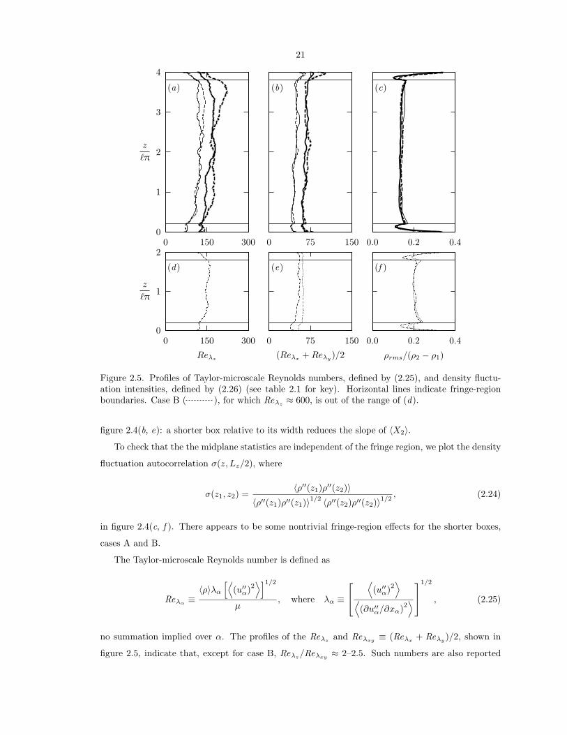
Figure 2.5. Profiles of Taylor-microscale Reynolds numbers, defined by (2.25), and density fluctu-ation intensities, defined by (2.26) (see table 2.1 for key). Horizontal lines indicate fringe-regionboundaries. Case B ( ), for which Reλz

≈ 600, is out of the range of (d).

figure 2.4(b, e): a shorter box relative to its width reduces the slope of 〈X2〉.

To check that the the midplane statistics are independent of the fringe region, we plot the density

fluctuation autocorrelation σ(z, Lz/2), where

σ(z1, z2) =〈ρ′′(z1)ρ′′(z2)〉

〈ρ′′(z1)ρ′′(z1)〉1/2 〈ρ′′(z2)ρ′′(z2)〉1/2, (2.24)

in figure 2.4(c, f ). There appears to be some nontrivial fringe-region effects for the shorter boxes,

cases A and B.

The Taylor-microscale Reynolds number is defined as

Reλα ≡〈ρ〉λα

[⟨(u′′α)2

⟩]1/2

µ, where λα ≡

⟨(u′′α)2

⟩⟨(∂u′′α/∂xα)2

⟩1/2

, (2.25)

no summation implied over α. The profiles of the Reλz and Reλxy ≡ (Reλx + Reλy )/2, shown in

figure 2.5, indicate that, except for case B, Reλz/Reλxy ≈ 2–2.5. Such numbers are also reported

22

in Cook and Dimotakis (2001), with Reλz/Reλxy ≈ 2.5–4, depending on the characteristic scale of

the initial conditions. In case B, however, Reλz/Reλxy ≈ 12, perhaps owing to the large eddy sizes

allowed by the horizontal extent of the computational domain. The general trend that Reλz/Reλxy

is higher with larger eddy sizes is also seen in Cook and Dimotakis (2001).

The root-mean-square (r.m.s.) density fluctuations at a constant-z plane is given by

ρrms(z) = 〈ρ′′ρ′′〉1/2. (2.26)

Its profiles for the tall boxes, but with different Re and A are plotted in figure 2.5(c). Outside the

fringe, the profiles take on roughly constant values, scaling with (ρ2− ρ1), regardless of A. In Cook,

Cabot and Miller (2004), an effective Atwood number Ae, defined at the center of the mixing zone

as ρrms/〈ρ〉, is shown to approach 0.48A at late times. Presently, 〈ρ〉z=Lz/2 ≈ ρ0 for all cases, and

so (Ae/A)z=Lz/2 = 2(ρrms)z=Lz/2/(ρ2−ρ1), ranging from 0.35 to 0.4, depending on the aspect ratio

of the computational domain.

2.4.2 Spectra

The planar spectra, E2Dρρ , −E2D

ρw , E2Duu , and E2D

vv , as defined by (2.22), at the midplane location,

are plotted in figures 2.6 and 2.7, nondimensionalized by their respective midplane Kolmogorov–

Obukhov–Corrsin (KOC) scales: specific kinetic energy dissipation ε, density fluctuation dissipation

ερ and kinematic viscosity ν, which we will define as

ε = ν

⟨(∂ui

∂xj

)2

+13

(∂ui

∂xi

)2⟩, ερ = D

⟨(∂ρ

∂xj

)2⟩, ν =

µ

〈ρ〉, (2.27)

whence η = (ν3/ε)1/4. Observe that, when plotted in KOC scaling, all the spectra from the present

simulations virtually collapse, especially in the high-wavenumber range, regardless of A, Re, and

Lz/Lx. This suggests that, in modeling spectra, the standard scaling ideas (Lumley 1967) used for

passive scalar mixing can still be applied to the active scalar mixing problem; in other words, ε, ερ,

and ν are still the relevant scales. Further, these spectra appear to approach the standard power-law

scaling with the −5/3 exponent for E2Dww and (E2D

uu + E2Dvv )/2, and the −7/3 exponent for −E2D

ρw .

Note that the E2Dρρ spectra appears to be slightly flatter than a −5/3 power law.

For comparison, we also show the 30723 DNS spectra from Cabot and Cook (2006) in figures

2.6 and 2.7, normalized by their constant-ν version of (2.27). We also ran a constant-ν, that is

µ(x, t) = νρ(x, t), version of the present flow simulations with no discernible differences in the

spectra. The present data allows the comparison of statistically evolving Rayleigh–Taylor spectra

relative to statistically stationary flow spectra at the same level of dissipation. When compared to the

Rayleigh–Taylor spectra, the present E2Dρρ and −E2D

ρw show near collapse but E2Dww and (E2D

uu +E2Dvv )/2

23

10−4

10−2

100

102

104

10−2 10−1 100

E2Dρρ ε3/4ε−1

ρ ν−5/4

−5/3

(a)

10−4

10−2

100

102

104

10−2 10−1 100

krη

−E2Dρw ε1/4ε

−1/2ρ ν−5/4

−7/3

(b)

Figure 2.6. Midplane spectra normalized by KOC scales (2.27) of (a) density and (b) density–vertical-velocity: , 30723 DNS of Rayleigh–Taylor instability (Cabot and Cook 2006); re-maining lines are from present simulations (see table 2.1 for key).

24

10−4

10−2

100

102

104

10−2 10−1 100

E2Dwwε−1/4ν−5/4

−5/3

(a)

10−4

10−2

100

102

104

10−2 10−1 100

krη

(1/2)(E2Duu + Evv)ε−1/4ν−5/4

−5/3

(b)

Figure 2.7. Midplane spectra normalized by KOC scales (2.27) of (a) vertical velocity and (b)horizontal velocity: , 30723 DNS of Rayleigh–Taylor instability (Cabot and Cook 2006);remaining lines are from present simulations (see table 2.1 for key).

25

are slightly higher in the high-wavenumber range. This is perhaps not surprising since turbulence

production is greater than dissipation in Rayleigh–Taylor turbulence whereas the present spectra

represent “equilibrium” buoyancy-driven turbulence. Even though they do not collapse completely,

they share common power-law slopes in the inertial range.

2.4.3 Mole Fraction Probability Density Functions

The probability density functions (p.d.f.) of X2, shown in figure 2.8, are taken at various vertical

locations: the left-most and right-most curves represent the p.d.f.s taken from the middle of the

lower and upper fringes, respectively, and the remaining curves are p.d.f.s taken from the quarter-,

half-, and three-quarter domain height. Outside the fringe regions, the p.d.f.s are roughly unimodal

with peaks varying from 0 to 1. An exception is case B (figure 2.8(b)), which exhibits bimodal

behavior, indicating the persistence of unmixed fluids. This can be attributed to the large eddies,

permitted by the large horizontal dimensions (figure 2.4(d)), that cause large-scale sloshing motions

as unmixed fluids clump together. In contrast, we observe better small-scale mixing when the eddies

are smaller (cases A, C–F).

All else equal, the A = 3/4 runs (figure 2.8(d, f )) exhibit wider p.d.f.s compared to the A = 1/2

runs (figure 2.8(c, e)). We also observe a slight skew toward lower X2 at the midplane location, seen

in figure 2.8(c–f ), consistent with the Rayleigh–Taylor turbulence LES performed by Cook, Cabot

and Miller (2004) (figure 13).

26

0

1

2

3

4

0 0.5 1

(a)

0 0.5 1

(b)

0

1

2

3

4

0 0.5 1

(c)

0 0.5 1

(d)

0

1

2

3

4

0 0.5 1

X2

(e)

0 0.5 1

X2

(f )

Figure 2.8. P.d.f.s of X2, defined by (2.23), taken from xy-planes located at, from left to right(alternating between solid and broken lines for legibility), z = 0.5Lf , 0.25Lz, 0.5Lz, 0.75Lz, andLz − 0.5Lf . (a) case A, (b) case B, (c) case C, (d) case D, (e) case E and (f ) case F.

27

Chapter 3

LES and SGS Modeling of ActiveScalar Mixing Flows

3.1 Background

Originally, researchers (e.g., Pullin 2000, Burton 2008) developed SGS models for turbulent flows

in which the scalar is passive. In this chapter, we extend the SGS passive scalar model of Pullin

(2000) to handle mildly active (buoyant) scalars. We refer the interested reader to Sagaut (2006)

for a review of other SGS active scalar models.

First, we define the relevant scale-dependent nondimensional parameters (see Shih et al. 2005,

Ivey et al. 2008):

Re` ≡U`

ν, Ri` ≡

N2

U2/`2, I ≡ ε

νN2,

where N is the Brunt–Vaisala frequency defined by N2 = −g(∂ρ/∂z); A is the Atwood number; g

is the gravitational acceleration; ∂ρ/∂z is the vertical (opposite to gravity) mean density gradient;

ε is the viscous dissipation; and U is characteristic velocity at scale `. If we further assume that

ε = U3/`, we have the following relations:

Re` =(`

η

)4/3

, Ri` =(

`

LO

)4/3

, I =Re`

Ri`=(LO

η

)4/3

,

where η = (ν3/ε)1/4, the Kolmogorov lengthscale and LO = (ε/N3)1/2, the Ozmidov lengthscale.

Eddies smaller than η are strongly dissipated by viscosity, and eddies larger than LO are strongly

suppressed by stratification through conversion to potential energy (Turner 1973). In other words,

the unrestrained turbulent eddies have sizes between η and LO; therefore, I = (LO/η)4/3 provides

a measure of turbulence activity. Brethouwer et al. (2007) call I the buoyancy Reynolds number.

Figure 3.1 summarizes the three mixing regimes described by Ivey, Winters and Koseff (2008).

When I < 7, the flow is both strongly stratified and dominated by viscosity—motion is quickly

suppressed. As I is increased, the flow first transitions before it becomes fully energetic when

28

SGS model

Re = (/η)4/3

102 104 106 108

Ri = (/LO)4/3

100

102

104

106 I = (LO/η)4/3 = 100

I = (LO/η)4/3 = 7

Molecular

Energetic

Figure 3.1. Flow regimes in stable stratification characterized by scale-dependent Ri` and Re`.Shaded area indicates the operating region for present SGS model extension.

I > 100, a process somewhat similar to the mixing transition (Dimotakis 2000). When Ri` 1 and

I 1, the energy spectrum E comprises a buoyancy subrange, E ∼ N2k−3 in k L−1O , and an

inertial subrange, E ∼ ε2/3k−5/3 in L−1O k η−1 (Turner 1973). Turbulence in the atmosphere

and ocean belong to this energetic regime.

When the flow is unstably stratified (also known as the Rayleigh–Taylor instability), the gradi-

ent Richardson number is negative, but its usual meaning—a measure of stratification relative to

turbulence production—is undefined since, for stationary–homogeneous flows, buoyancy flux is the

only source of turbulent kinetic energy and is therefore equal to the dissipation. In the context of

SGS modeling, the effects of buoyancy have already been accounted for once the dissipation, readily

determined from matching structure functions at the cutoff scale, is known. In this regime, the usual

SGS models of Misra and Pullin (1997), Pullin (2000) are adequate. We demonstrate that this is

indeed the case in § 3.2 by performing LES of the unstably stratified flow described in chapter 2.

For stable stratification, we present a new SGS model for the dynamics of the inertial range,

L−1O k η−1 (shaded region in figure 3.1). In this range, stratification alters the overall turbulent

kinetic energy available for mixing and dissipation, but the Richardson cascade, characterized by

this altered kinetic energy, is still preserved. In this sense, the scalar is deemed mildly active. To

model this effect, we develop a first-order buoyancy correction to the SGS passive scalar flux model

of Pullin (2000) in § 3.3. We expect that, using this SGS model, one is able to simulate, with reduced

computations, fully developed stratified turbulence by directly simulating the eddies with sizes down

to LO while modeling the eddies with sizes from LO down to η.

29

3.2 LES of Unstably Stratified Flow

We perform 32 × 32 × 64, 64 × 64 × 128, and 128 × 128 × 256 LES of the DNS case E (table 2.1),

which was run on a 384×384×768 grid. We refer the reader to chapter 2 for full details of the DNS

and flow setup. We only present LES-specific details in this chapter.

3.2.1 Filtered LES Equations and SGS Model

Following Mattner, Pullin and Dimotakis (2004), Hill, Pantano and Pullin (2006), we filter the

governing equations in the form (2.1), (2.2) and (2.3), and then rearrange them using

1/ρ = Y1/ρ1 + (1− Y1)/ρ2 (3.1)

to obtain:

∂uj

∂xj= −D ∂

2s

∂x2j

+∂qs

j

∂xj− ωs, (3.2a)

∂s

∂t+ uj

∂s

∂xj= D ∂

2s

∂x2j

−∂qs

j

∂xj+ ωs, (3.2b)

∂ui

∂t+ uj

∂ui

∂xj= −1

ρ

(∂p

∂xi+ Γi

)+

1ρ

∂τij∂xj

− 1ρ

∂ρTij

∂xj− gδi3, (3.2c)

where s ≡ log(ρ/ρ0). Given a field φ(x), we define its Favre-average by φ ≡ ρφ/ρ; this, in turn, is

defined by the LES filter associated with cutoff scale ∆c,

φ(x) =∫G(x− x′;∆c)φ(x′) dx′.

The subgrid stress tensor is given by (Misra and Pullin 1997)

Tij = (δij − evi e

vj )K, (3.3)

and we choose the subgrid vortex to align with the most extensive eigenvector of the strain-rate

tensor, ev = eeS . K is the subgrid (specific) kinetic energy, given by

K =∫ ∞

kc

E(κ) dκ, (3.4)

where kc ≡ π/∆c and ∆c = ∆x = ∆y = ∆z. The energy spectrum of a spiral vortex is

E(κ) = K0ε2/3κ−5/3 exp

[−κ2λ2

v

], (3.5)

30

where λ2v = 2ν/(3|a|); ν = µ/ρ; and a = ev

i evj Sij , so that

K =12K′0Γ[−1/3, k2

cλ2v], where K′0 = K0ε

2/3λ2/3v . (3.6)

We determine K′0 by matching an expression for the SGS model structure function with its observed

value computed from the resolved part of the LES simulation (Pullin 2000, Voelkl, Pullin and Chan

2000, Hill, Pantano and Pullin 2006).

Since the filter is applied to the Y1 equation, (2.1), we model its (specific) flux as if it were a

passive scalar (Pullin 2000, Hill, Pantano and Pullin 2006):

qY1i ≡ Y1ui − Y1ui = −γY1

∆c

2K1/2(δij − ev

i evj )∂Y1

∂xj; (3.7)

presently, γY1 = 1. Upon substituting (3.1) into (3.7) and comparing the result with both the filtered

form of (2.1) and (3.2 b), we find that

qsi ≡ ui − ui ≡ −

(1ρ1− 1ρ2

)ρqY1

i = −γY1

∆c

2K1/2(δij − ev

i evj )∂s

∂xj.

We can rearrange this to relate the subgrid mass flux, ρui, to the resolved density gradient, ∂ρ/∂xi:

ρui − ρ ui = −γY1

∆c

2K1/2(δij − ev

i evj )∂ρ

∂xj. (3.8)

By definition, the above quantity is equal to∫∞

kcEρui

(κ; ev) dκ, where Eρuiis the ρ–ui cospectrum

of the two-dimensional flow in the ev-oriented vortex cross section. After substituting (3.4) and

(3.5) into (3.8), we solve for Eρuito get

Eρui(κ; ev) = −γY1(2/3)1/2π(K′0)1/2λ2

vF (κλv)(δij − evi e

vj )∂ρ

∂xj, (3.9)

where

F (κv) =√

34κ−7/3

v

(e−κ2v + κ

2/3v Γ[−1/3, κ2

v])

(κ2/3v Γ[−1/3, κ2

v])1/2.

In the inertial range (κv → 0), F ∼ κ−7/3v . Equation (3.9) is consistent with the well-known

result obtained from scaling arguments (e.g., Lumley 1967, Saddoughi and Veeravalli 1994) that

Eρu(κ) ∼ −(∂ρ/∂x)ε1/3κ−7/3.

31

3.2.2 Subgrid Extensions of Planar Spectra

Assuming that the subgrid vortices are aligned according to delta-function p.d.f.s with peaks at

ev(x) = (sinα0 cosβ0, sinα0 sinβ0, cosα0),

we use the following expressions, given by Hill, Pantano and Pullin (2006) (equations (6.11) and

(6.12)), to obtain xy-plane velocity spectra from the vortex spectrum (see also Pullin and Saffman

1994):

E2Dqq (kr) =

2kr

π

∫ |kr/ cos α0|

kr

E(κ)(κ2 − k2

r)1/2(k2r − κ2 cos2 α0)1/2

dκ, (3.10a)

E2D33 (kr) =

2kr

π

∫ |kr/ cos α0|

kr

(k2r − κ2 cos2 α0)1/2E(κ)κ2(κ2 − k2

r)1/2dκ, (3.10b)

where kr = (k2x +k2

y)1/2, the radial wavenumber; and E(κ) is given by (3.5). In the present notation,

(E2Duu + E2D

vv )/2 = E2Dqq − E2D

33 and E2Dww = 2E2D

33 . A similar expression can be found for the planar

ρ–ui cospectrum (see appendix A):

E2Dρui

(kr) =2kr

π

∫ |kr/ cos α0|

kr

Eρui(κ; ev)

(κ2 − k2r)1/2(k2

r − κ2 cos2 α0)1/2dκ, (3.11)

where Eρui(κ; ev) is given by (3.9). Given kr and z, we average (3.10) and (3.11) across the xy-plane

to obtain subgrid extensions of planar spectra.

We plot in figure 3.2 the midplane (z = Lz/2) resolved-scale spectra and their subgrid extensions,

normalized by ν ≡ µ/〈ρ〉 and ε′ ≡ 〈Sijτij − ρSijTij〉/〈ρ〉, where 〈 〉 denotes the xy-plane average.

The LES spectra are in general agreement with their DNS counterparts, also shown in figure 3.2.

However, the subgrid extensions show noticeable resolution dependence at the viscous rolloff. This

can be understood as follows: the viscous rolloff is determined by the factor exp[−2νκ2/(3|a|)] in

the model energy spectrum, (3.5), but the local strain rate a is itself an LES resolution-dependent

quantity. Since we expect that the energy transfer off the resolved-scale grid to subgrid scales will,

in general, depend on the LES-resolution, then this approximation is acceptable and necessary for

integrating the resolved-scale variables in time. For the purposes of subgrid extension, however, a

different approximation is appropriate.

Following Lundgren (1982), we estimate that a = (ε/(15ν))1/2, where ε is the local cell-averaged

dissipation rate to be determined. With this estimate, the viscous rolloff is now characterized by

the resolution-independent factor exp[−(1.61η)2κ2] in (3.5), where η = (ν3/ε)1/4. To determine ε,

we solve the following transcendental equation, obtained from (3.3), (3.6), and the definitions of ε

32

10−4

10−2

100

102

104

10−2 10−1 100

(E2Duu + E2D

vv )/2ε′1/4ν5/4

E2Dww

ε′1/4ν5/4

−5/3

(a)

10−2

100

102

104

106

10−2 10−1 100

krη

−E2Dρw ε′1/4ν−7/4〈∂ρ/∂z〉−1

−7/3

(b)

Figure 3.2. LES and DNS comparisons of (a) midplane vertical-velocity spectra and horizontal-velocity spectra and (b) midplane density–vertical-velocity cospectra: , 32 × 32 × 64 LES; ,64×64×128 LES; , 128×128×256 LES; open symbols, resolved; solid symbols, subgrid; ,384× 384× 768 DNS (case E from table 2.1).

33

and η:

ε = Sijτij/ρ− Sij(δij − evi e

vj )

12A(1.61η)2/3Γ[−1/3, (1.61η)2k2

c ],

η = (ν3/ε)1/4,

(3.12)

where A is the inseparable group prefactor K0ε2/3 determined from the structure function matching

procedure. Equation (3.12), analogous to (37) in Pullin and Saffman (1993), merely states that the

local cell-averaged dissipation comprises the resolved and subgrid components. Having determined

ε, we can then calculate the subgrid extensions as before but replacing λv = 1.61η in both (3.5) and

(3.9).

We replot in figure 3.3(a) the midplane resolved-scale velocity spectra and their subgrid exten-

sions, now normalized by ν and ε, where ν ≡ µ/〈ρ〉 as before, but now ε = 〈ε〉, different from ε′. The

general features of the LES spectra are in fair agreement with their DNS counterparts. However,

LES slightly underpredicts both the vertical-velocity spectrum, E2Dww, and the horizontal-velocity

spectrum, (E2Duu + E2D

vv )/2, at around krη = 10−1. Observe that the improved subgrid extensions

now collapse. The ρ–w cospectra, normalized by ν, ε, and 〈∂ρ/∂z〉, are shown in figure 3.3(b). The

resolved part of the LES cospectra agree well with DNS and their subgrid extensions accurately

capture the shape and location of the viscous rolloff, independent of the LES resolution. We remark

that in the subgrid estimation, ε is to be viewed as a random variable whose planar/timewise p.d.f. is

determined by the LES itself. Pullin and Saffman (1993) argue that the effect of statistical variation

of the effective strain can change the −κ2 factor within the exponential of the Lundgren spectrum

to −κ, as is observed in experiment and DNS. This effect can be seen in the present subgrid-scale

extension, figure 3.4, a result that compares well with the high-Re experiments of Saddoughi and

Veeravalli (1994), in which it was reported that E(k) ∝ exp(−5.2kη) in the range 0.5 < kη < 3.

Plotting the velocity-anisotropy parameter E2Dww/E

2Duiui

− 1/3 in figure 3.5(a), we observe that

the present LES captures the small-scale anisotropy observed in DNS. In particular, the decreasing

anisotropy from low wavenumbers up to krη = 10−1, followed by a gradually increasing anisotropy

up to krη = 2 is reported by both DNS and LES. For the LES, the location of the minimum is

independent of the LES resolution. It appears from figure 3.5(a) that the anisotropy increases

indefinitely, albeit gradually, with increasing wavenumber. We superimpose the high-resolution

Rayleigh–Taylor DNS velocity-anisotropy parameter from Cabot and Cook (2006) in figure 3.5(b)

to see that the anisotropy eventually decreases after reaching a local maximum of about 0.18 at

krη = 2.

That the anisotropy increases with wavenumber is perhaps counterintuitive, and perhaps con-

tradictory to the notion of small-scale isotropy. We remark that Cabot and Cook (2006) measured

small-scale anisotropy by comparing the relative magnitudes of directional Kolmogorov microscales,

defined by ηi = (ν3/εi)1/4, εi = 15ν〈(∂ui/∂xi)2〉 (no summation), and found that, with this measure,

the small scales were isotropic. A question then arises as to why the velocity-anisotropy parameter

34

10−4

10−2

100

102

104

10−2 10−1 100

(E2Duu + E2D

vv )/2ε1/4ν5/4

E2Dww

ε1/4ν5/4

−5/3

(a)

10−2

100

102

104

106

10−2 10−1 100

krη

−E2Dρw ε1/4ν−7/4〈∂ρ/∂z〉−1

−7/3

(b)

Figure 3.3. Improved subgrid extensions in LES and DNS comparisons of (a) midplane vertical-velocity spectra and horizontal-velocity spectra and (b) midplane density–vertical-velocity cospectra: , 32× 32× 64 LES; , 64× 64× 128 LES; , 128× 128× 256 LES; open symbols, resolved; solidsymbols, subgrid; , 384× 384× 768 DNS (case E from table 2.1).

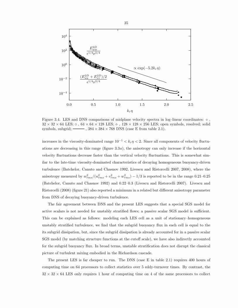
35

10−4

10−2

100

102

104

0.0 0.5 1.0 1.5 2.0 2.5

krη

(E2Duu + E2D

vv )/2ε1/4ν5/4

E2Dww

ε1/4ν5/4

∝ exp(−5.2krη)

Figure 3.4. LES and DNS comparisons of midplane velocity spectra in log–linear coordinates: ,32 × 32 × 64 LES; , 64 × 64 × 128 LES; , 128 × 128 × 256 LES; open symbols, resolved; solidsymbols, subgrid; , 384× 384× 768 DNS (case E from table 2.1).

increases in the viscosity-dominated range 10−1 < krη < 2. Since all components of velocity fluctu-

ations are decreasing in this range (figure 3.3a), the anisotropy can only increase if the horizontal

velocity fluctuations decrease faster than the vertical velocity fluctuations. This is somewhat sim-

ilar to the late-time viscosity-dominated characteristics of decaying homogeneous buoyancy-driven

turbulence (Batchelor, Canuto and Chasnov 1992, Livescu and Ristorcelli 2007, 2008), where the

anisotropy measured by w2rms/(u

2rms + v2

rms + w2rms)− 1/3 is reported to be in the range 0.21–0.25

(Batchelor, Canuto and Chasnov 1992) and 0.22–0.3 (Livescu and Ristorcelli 2007). Livescu and

Ristorcelli (2008) (figure 21) also reported a minimum in a related but different anisotropy parameter

from DNS of decaying buoyancy-driven turbulence.

The fair agreement between DNS and the present LES suggests that a special SGS model for

active scalars is not needed for unstably stratified flows; a passive scalar SGS model is sufficient.

This can be explained as follows: modeling each LES cell as a unit of stationary–homogeneous

unstably stratified turbulence, we find that the subgrid buoyancy flux in each cell is equal to the

its subgrid dissipation, but, since the subgrid dissipation is already accounted for in a passive scalar

SGS model (by matching structure functions at the cutoff scale), we have also indirectly accounted

for the subgrid buoyancy flux. In broad terms, unstable stratification does not disrupt the classical

picture of turbulent mixing embodied in the Richardson cascade.

The present LES is far cheaper to run. The DNS (case E in table 2.1) requires 400 hours of

computing time on 64 processors to collect statistics over 5 eddy-turnover times. By contrast, the

32 × 32 × 64 LES only requires 1 hour of computing time on 4 of the same processors to collect

36

0.0

0.1

0.2

0.3

0.4

0.5

0.6

10−2 10−1 100

E2Dww

E2Duu + E2D

vv + E2Dww

− 13

(a)

0.0

0.1

0.2

0.3

0.4

0.5

0.6

10−2 10−1 100

krη

E2Dww

E2Duu + E2D

vv + E2Dww

− 13

(b)

Figure 3.5. LES and DNS comparisons of the midplane velocity-anisotropy parameter: , 32×32×64LES; , 64× 64× 128 LES; , 128× 128× 256 LES; open symbols, resolved; solid symbols, subgrid;

, 384 × 384 × 768 DNS (case E from table 2.1); , 30723 DNS of Rayleigh–Taylorinstability (Cabot and Cook 2006).

37

statistics over 23 eddy-turnover times. In terms of processor-hours per 10 eddy-turnover times, this

represents savings by a factor in excess of 105.

3.3 SGS Model for Stably Stratified Flows

The development of the SGS model for active scalar flux in a stably stratified flow is organized

as follows. In § 3.3.1, we introduce the vortex-based model for active scalar dynamics by invoking

assumptions similar to that used by Pullin (2000). We then perform a perturbation expansion for

small Richardson numbers (mildly active scalar) of the model equations in § 3.3.2. The solution

to the perturbation equations was then used to calculate the Ri-dependent corrections to the SGS

kinetic energy (§ 3.3.3) and SGS scalar flux (§ 3.3.4). Finally, we use the DNS data of chapter 2 to

perform an a posteriori testing of the new active scalar SGS model in § 3.3.5.

3.3.1 Vortex-Based SGS Model for Active Scalar Dynamics

To simplify the analysis, we will use the Boussinesq approximation of the governing equations. First,

expand the flow variables in small Atwood number A,

s = As(1) +O(A2), ui = u(0)i +O(A), p = p(0) +O(A),

and then substitute these expansions into the governing equations, (2.6), (2.7), and (2.16), omitting

the source term ωs. Collecting leading-order terms while maintaining Ag = O(1) gives the Boussinesq

form of the governing equations:

∂s(1)

∂t+ u

(0)j

∂s(1)

∂xj= D∂

2s(1)

∂x2j

,

∂u(0)j

∂xj= 0,

∂u(0)i

∂t+ u

(0)j

∂u(0)i

∂xj= − ∂P

∂xi+ ν

∂2u(0)j

∂x2j

−Ags(1)δi3,

(3.13)

where ν = µ/ρ0, P = (p(0) + ρ0gx3)/ρ0. We will henceforth drop the cumbersome superscripts, and

rename As(1) → c. Taking the curl of the momentum equation in (3.13), we obtain the vorticity

equation that contains a buoyancy source (or sink):

∂ωi

∂t+ uj

∂ωi

∂xj= ωj

∂ui

∂xj+ ν

∂2ωi

∂x2j

− gεij3∂c

∂xj. (3.14)

Following the simplified analysis of Pullin (2000), we model the SGS dynamics of a turbulent flow

fields as an ensemble of idealized flows, each of which is a two-dimensional two-component (xy-plane)

38

inviscid vortex (ν = 0) in an immiscible (D = 0) fluid. In addition, these flows are now subjected

to gravity, which now, without loss of generality, points in the −y direction of the vortex frame.

In polar coordinates, the governing equations for the active scalar c(r, θ, t), out-of-plane vorticity

ω(r, θ, t), and streamfunction ψ(r, θ, t) are

∂c

∂t+

1r

(∂ψ

∂θ

∂c

∂r− ∂c

∂θ

∂ψ

∂r

)= 0,

∂ω

∂t+

1r

(∂ψ

∂θ

∂ω

∂r− ∂ω

∂θ

∂ψ

∂r

)= −g

(∂c

∂rcos θ − 1

r

∂c

∂θsin θ

),

ω = −(

1r

∂

∂rr∂

∂r+

1r2

∂2

∂θ2

)ψ,

(3.15)

with initial conditionsc(r, θ, 0) =

∂c

∂xr cos θ +

∂c

∂yr sin θ,

ω(r, θ, 0) =1r

ddrr2Ω(r).

(3.16)

where x = r cos θ and y = r sin θ. Ω(r), ∂c/∂x, and ∂c/∂y characterize the resolved vorticity and

the resolved scalar gradient. This simplified vortex model now incorporates the buoyancy source—

compare (3.14) and (3.15).

The relevant nondimensional parameter in this problem is the Richardson number

Ri ≡ −g(∂c/∂y)1/T 2

, (3.17)

where T is the eddy-turnover time of the subgrid vortex described by Ω. When the flow is stably

stratified, Ri > 0.

3.3.2 Perturbation Expansion of Mildly Active Scalar Equations

Now, consider the case when the scalar is mildly active, |Ri | 1. This occurs when the size of

the vortex is small relative to the Ozmidov scale LO. We can then perform a regular perturbation

expansion in small Ri, or equivalently, small g, in which case, g is understood to be small relative

to (∂c/∂y)−1T−2:

c = c(0) + gc(1) +O(g2), ω = ω(0) + gω(1) +O(g2), ψ = ψ(0) + gψ(1) +O(g2). (3.18)

39

Substituting (3.18) into (3.15) and (3.16), then collecting O(g0) terms, we obtain

∂c(0)

∂t+

1r

(∂ψ(0)

∂θ

∂c(0)

∂r− ∂c(0)

∂θ

∂ψ(0)

∂r

)= 0,

∂ω(0)

∂t+

1r

(∂ψ(0)

∂θ

∂ω(0)

∂r− ∂ω(0)

∂θ

∂ψ(0)

∂r

)= 0,

ω(0) = −(

1r

∂

∂rr∂

∂r+

1r2

∂2

∂θ2

)ψ(0),

with initial conditions

c(0)(r, θ, 0) =∂c

∂xr cos θ +

∂c

∂yr sin θ,

ω(0)(r, θ, 0) =1r

ddrr2Ω(r).

As expected, the O(g0) equations are the passive scalar equations. We immediately write its solution,

c(0)(r, θ, t) =∂c

∂xr cos(θ − Ωt) +

∂c

∂yr sin(θ − Ωt),

ω(0)(r, θ, t) =1r

ddrr2Ω,

∂ψ(0)

∂r(r, θ, t) = −rΩ,

(3.19)

which can be verified by direct substitution. This is the same as the solution obtained by Pullin

(2000). Physically, (3.19) represents the convective action of the vortex, winding the linear scalar

gradient into tight spirals, effectively flattening the mean scalar gradient, and results in a counter-

gradient subgrid scalar flux.

The equations for the first-order correction can be obtained by collecting O(g1) terms in the

perturbation expansion, giving

∂c(1)

∂t+ Ω

∂c(1)

∂θ+

1r

(∂ψ(1)

∂θ

∂c(0)

∂r− ∂c(0)

∂θ

∂ψ(1)

∂r

)= 0,

∂ω(1)

∂t+ Ω

∂ω(1)

∂θ+

1r

(∂ψ(1)

∂θ

∂ω(0)

∂r− ∂ω(0)

∂θ

∂ψ(1)

∂r

)= −

(∂c(0)

∂rcos θ − 1

r

∂c(0)

∂θsin θ

),

ω(1) = −(

1r

∂

∂rr∂

∂r+

1r2

∂2

∂θ2

)ψ(1),

(3.20)

with initial conditions

c(1)(r, θ, 0) = 0, ω(1)(r, θ, 0) = 0.

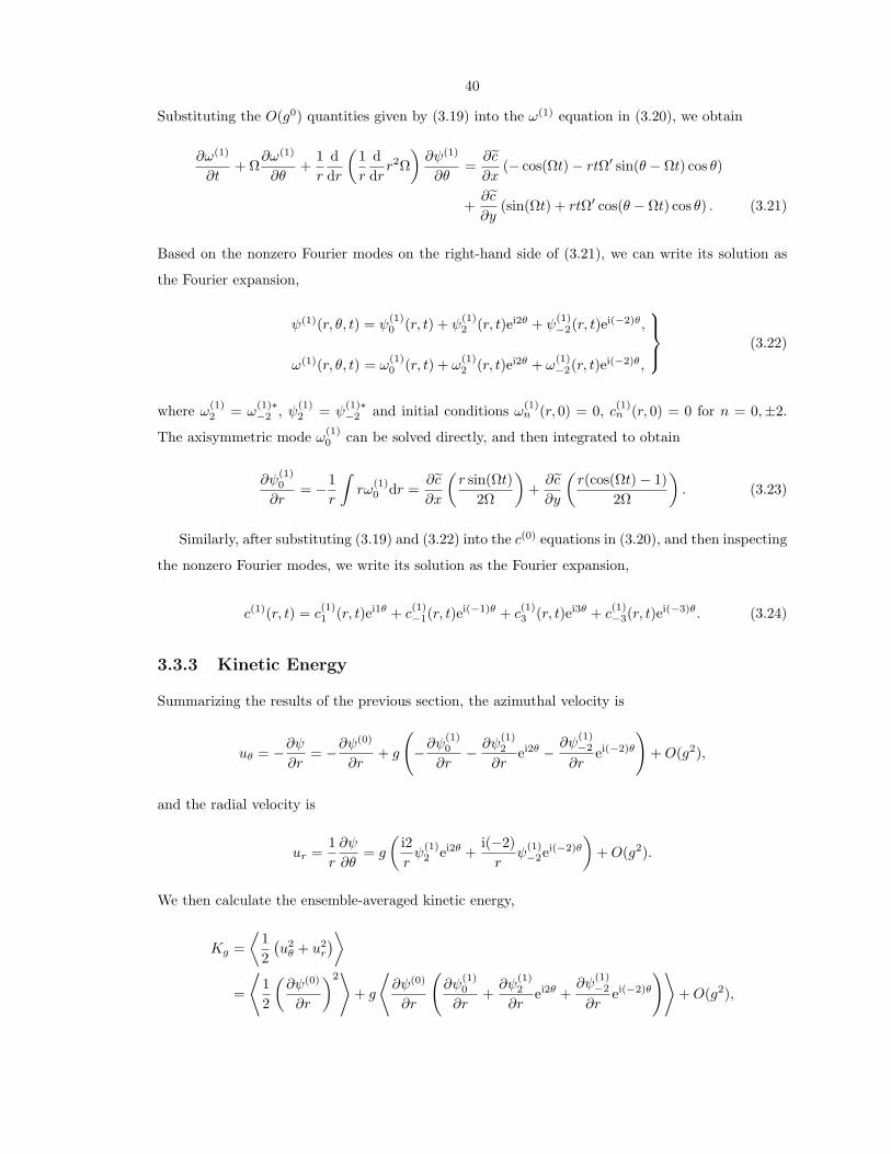
40

Substituting the O(g0) quantities given by (3.19) into the ω(1) equation in (3.20), we obtain

∂ω(1)

∂t+ Ω

∂ω(1)

∂θ+

1r

ddr

(1r

ddrr2Ω

)∂ψ(1)

∂θ=∂c

∂x(− cos(Ωt)− rtΩ′ sin(θ − Ωt) cos θ)

+∂c

∂y(sin(Ωt) + rtΩ′ cos(θ − Ωt) cos θ) . (3.21)

Based on the nonzero Fourier modes on the right-hand side of (3.21), we can write its solution as

the Fourier expansion,

ψ(1)(r, θ, t) = ψ(1)0 (r, t) + ψ

(1)2 (r, t)ei2θ + ψ

(1)−2(r, t)ei(−2)θ,

ω(1)(r, θ, t) = ω(1)0 (r, t) + ω

(1)2 (r, t)ei2θ + ω

(1)−2(r, t)ei(−2)θ,

(3.22)

where ω(1)2 = ω

(1)∗−2 , ψ(1)

2 = ψ(1)∗−2 and initial conditions ω(1)

n (r, 0) = 0, c(1)n (r, 0) = 0 for n = 0,±2.

The axisymmetric mode ω(1)0 can be solved directly, and then integrated to obtain

∂ψ(1)0

∂r= −1

r

∫rω

(1)0 dr =

∂c

∂x

(r sin(Ωt)

2Ω

)+∂c

∂y

(r(cos(Ωt)− 1)

2Ω

). (3.23)

Similarly, after substituting (3.19) and (3.22) into the c(0) equations in (3.20), and then inspecting

the nonzero Fourier modes, we write its solution as the Fourier expansion,

c(1)(r, t) = c(1)1 (r, t)ei1θ + c

(1)−1(r, t)e

i(−1)θ + c(1)3 (r, t)ei3θ + c

(1)−3(r, t)e

i(−3)θ. (3.24)

3.3.3 Kinetic Energy

Summarizing the results of the previous section, the azimuthal velocity is

uθ = −∂ψ∂r

= −∂ψ(0)

∂r+ g

(−∂ψ

(1)0

∂r− ∂ψ

(1)2

∂rei2θ −

∂ψ(1)−2

∂rei(−2)θ

)+O(g2),

and the radial velocity is

ur =1r

∂ψ

∂θ= g

(i2rψ

(1)2 ei2θ +

i(−2)r

ψ(1)−2ei(−2)θ

)+O(g2).

We then calculate the ensemble-averaged kinetic energy,

Kg =⟨

12(u2

θ + u2r

)⟩=

⟨12

(∂ψ(0)

∂r

)2⟩

+ g

⟨∂ψ(0)

∂r

(∂ψ

(1)0

∂r+∂ψ

(1)2

∂rei2θ +

∂ψ(1)−2

∂rei(−2)θ

)⟩+O(g2),

41

where the average is taken over space, time and the sign of Ω:

〈 〉 =12

∑sgn Ω

1T

∫ T

0

1πR2

1

∫ 2π

0

∫ R1

0

( ) r dr dθ dt,

where T is the vortex eddy-turnover time and R1 is the vortex size. The θ-integral removes terms

containing the factor enθ for n 6= 0, therefore simplifying Kg to

Kg =

⟨12

(∂ψ(0)

∂r

)2⟩

+ g

⟨∂ψ(0)

∂r

∂ψ(1)0

∂r

⟩+O(g2).

Substituting the solutions, (3.19) and (3.23), we obtain

Kg =1R2

1

∫ R1

0

r3Ω2 dr + g∂c

∂y

1R2

1

∫ R1

0

r3(− sin(ΩT ) + ΩT )ΩT

dr +O(g2).

Next, we rescale variables according to

Ω(r) =ΓR2

Ω(ξ), ξ =r

R, σ =

ΓTR2

,

where R ≤ R1 and σ = O(1), to write

Kg =Γ2

R21

∫ R1/R

0

ξ3Ω2 dξ + g∂c

∂y

R4

R21

∫ R1/R

0

ξ3(− sin(σΩ) + σΩ)

σΩdξ +O(g2).

The dominant contribution to the second integral comes near ξ = R1/R because the integrand

contains the ξ3 factor, which is small near ξ = 0. Since Ω(R1/R) 1 for a compact vortex, we

can replace the sine with its series expansion about its origin, and then collect terms to obtain the

simple expression

Kg ∼ Kv(1−Ri/6), where Kv =Γ2

R21

∫ R1/R

0

ξ3Ω2 dξ. (3.25)

Kv is the vortex kinetic energy for the passive scalar model (Pullin 2000) and Ri is defined in

(3.17). When a flow is stably stratified (Ri > 0), (3.25) says that the kinetic energy is reduced as

countergradient motion is converted into potential energy, and vice versa.

3.3.4 Scalar Flux

We calculate the ensemble-averaged scalar flux (fx, fy):

fx + ify ≡ 〈cu〉+ i〈cv〉 = 〈cureiθ〉+ 〈cuθieiθ〉.

42

Substituting the O(g0) solution, (3.19), and the O(g1) Fourier expansions, (3.22) and (3.24), and

then dropping the terms containing enθ for n 6= 0, we write

fx + ify =⟨

12iCeiΩtr2Ω

⟩+ g

(⟨−i C∗e−iΩtψ

(1)−2

⟩+⟨ic(1)−1rΩ

⟩+

⟨−1

2irC∗

∂ψ(1)−2

∂re−iΩt

⟩+

⟨−1

2irC ∂ψ

(1)0

∂reiΩt

⟩)+O(g2). (3.26)

where

C =∂c

∂x+ i

∂c

∂y.

We further assume that the phases of the nonaxisymmetric modes, argψ(1)−2 and arg c(1)−1, are ran-

dom (uniformly distributed in the range 0–2π), and therefore vanish under the ensemble average

〈 〉. The remaining terms in (3.26) represent the scalar flux resulting from the interaction between

the O(g0) scalar field and the collective effects of the O(g0) axisymmetric vorticity and its O(g1)

correction. After ensemble-averaging, rescaling and expanding trigonometric functions under the

integrals, (3.26) becomes

fx + ify = −12KvTC + g

(−iR2

1T

16C ∂c∂x

+iT 3Kv

48C(

4∂c

∂x+ i3

∂c

∂y

))+O(g2),

Substitute T = γ∆/K1/2v and further assume that R1 = γ∆, where γ = O(1), to get

fx = −12γ∆K1/2

v∂c

∂x

[1 +Ri

(−1

6

)],

fy = −12γ∆K1/2

v∂c

∂y

[1 +Ri

(−1

8+ζ2

24

)],

(3.27)

where ζ = (∂c/∂x)/(∂c/∂y) and Ri = −g(∂c/∂y)∆2/Kv; we set γ = 1 in the correction terms.

According to (3.27), the active scalar flux is reduced when the fluid is stably stratified (Ri > 0).

However, the size of the coefficients multiplying Ri in (3.27) suggests that the first-order corrections

are small.

3.3.5 A Posteriori Testing of Active Scalar SGS Model

The DNS data of chapter 2 provides an opportunity to test our SGS model (3.27) for active scalar

mixing in LES. Considered as part of a multiscale framework, each of the DNS simulations can be

viewed as a unit of statistically stationary turbulence found in an LES cell embedded in a density

gradient.

Even though we have argued that the buoyancy corrections are only useful for stably stratified

flows (Ri > 0), the terms in (3.27) are still defined when Ri < 0, and we can certainly set Ri = 0

43

0.0

0.5

1.0

1.5

2.0

10−2 10−1 100

kcη

γY1

Figure 3.6. Normalized scalar flux using passive scalar SGS model, given by (3.29) with Ri = 0. Seetable 2.1 for key.

for passive scalars.

Recasting (3.27) into the framework of chapter 2, (also compare with (3.8)), we have

〈ρ′′w′′〉c = −γY1

∆c

2K1/2 ∂〈ρ〉c

∂z

(1− Ri

8

), (3.28)

where gravity points in the −z direction; Y1 is the scalar; 〈 〉c is interpreted as the xy-plane LES

filter associated with the cutoff scale ∆c (≡ π/kc), formally defined as

〈f ′′g′′〉c =∫ ∞

kc

E2Dfg (kr) dkr,

kr = (k2x + k2

y)1/2; Ri = −(g/〈ρ〉c)(∂〈ρ〉c/∂z)∆2c/K; and K = 〈u′′i u′′i 〉c/2 is the subgrid (specific)

kinetic energy. Pullin (2000) estimated that γY1 = 0.89–1.3. Solving for γY1 ,

γY1(kc) =−〈ρ′′w′′〉c

(∆c/2) (〈u′′i u′′i 〉c/2)1/2 (∂〈ρ〉c/∂z) (1−Ri/8), (3.29)

which can be interpreted as the normalized subgrid scalar flux.

Plotting γY1(kc) using Ri = 0 at the midplane location (z = Lz/2) for all the DNS simulations

in figure 3.6, we observe that, in agreement with the analysis by Pullin (2000), γ = O(1) and is

roughly constant with values in the range 1.2–1.8 over one decade of wavenumbers before dropping

to zero when kcη > 1. This is rather surprising, since we have applied a passive scalar model to

an active scalar with moderately high density ratios, R = 3, 7. A possible explanation is that,

44

0.0

0.5

1.0

1.5

2.0

10−2 10−1 100

kcη

γY1

Figure 3.7. Normalized scalar flux using active scalar SGS model, given by (3.29). See table 2.1 forkey.

regardless of R, the present simulations of unstably stratified flows are still rate limited by turbulent

mixing, which is a key argument used in the development of the passive scalar flux model. One could

imagine a different outcome in a stably stratified configuration (Ri > 0), where stable stratification

overwhelms turbulent mixing by converting kinetic energy related to countergradient motion into

potential energy, effectively damping the flow.

We also plot (3.29) with the Ri corrections in figure 3.7, showing that, as expected, γY1(kc)

remains relatively unchanged, compared to figure 3.6, which did not have the buoyancy corrections.

45

Chapter 4

LES and Wall Modeling ofWall-Bounded Turbulence

4.1 Background

The idea of LES—directly simulating the large eddies while modeling the small eddies—cannot be

applied near walls in a straightforward way. Near walls, “large eddies”, implicitly defined by the

coarse grid, simply do not exist (Pope 2004). The near-wall eddies, having sizes constrained by the

wall, become underresolved at high Re and are therefore considered part of the subgrid motion. In

unbounded flows, the large eddies, carrying most of the turbulent kinetic energy, set the lengthscales

and timescales that describe the rest of the small-scale turbulence. This picture is reversed near the

wall, where the most energetically productive eddies are necessarily part of the small-scale motion.

Further, both these descriptions are present in wall-bounded flows, and both contribute significantly

to the overall turbulent flow field. This was demonstrated by Hutchins and Marusic (2007b), who

plotted velocity spectra of high-Re boundary layers at various wall distances and showed the existence

of two distinct energetic peaks: one that scales with viscous units, another that scales with boundary

layer thickness. Guided by even higher Re experiments (Mathis, Hutchins and Marusic 2009), they

later revised the location of the outer peak to scale as z ∼ Re1/2τ . A related complication is that,

given sufficiently high Re, even the mean velocity gradient is too steep to be resolved on the coarse

LES grid, appearing as a numerical discontinuity. The jump conditions across this discontinuity

depend on unclosed turbulent stresses, which themselves require reliable models.

One can always perform a partially resolved LES, where the near-wall grid is refined to resolve

the near-wall eddies (e.g., Voelkl, Pullin and Chan 2000). Although this kind of simulation has

its role in the development of LES models, its resolution requirement, which scales as O(Re1.8)

(Piomelli 2008), is almost as restrictive as DNS. But if we require that the resolution requirements

of LES be at most weakly dependent on Re, we are forced to explicitly model the vigorous near-wall

fluctuations and the numerical discontinuity (slip) in the mean velocity profile. Ample experimental

46

evidence that suggests some degree of universality in wall-bounded flows, e.g., the empirical log law

of the wall, offers hope that a viable LES wall model could be found.

Past modeling efforts were focussed on fitting a log law to the near-wall filtered velocity to obtain

the implied wall shear stress, which, in turn, is used as a wall stress boundary condition (Cabot and

Moin 1999, Pantano et al. 2008). Instead of the log law, the thin boundary layer equations (TBLEs)

coupled with a damped mixing-length eddy viscosity can also be used, giving good agreement with

experiments even in separating flows (Cabot and Moin 1999, Wang and Moin 2002). Yet another

method of determining the wall stress is by matching the LES eddy viscosity with the Reynolds-

averaged Navier–Stokes (RANS) eddy viscosity (Templeton, Medic and Kalitzin 2005), with success

at high Re.

We do not attempt to describe each of these methods in detail, but we will highlight some of these

efforts to provide a sample of the prevalent ideas in the field. Pantano et al. (2008) used 800×302×64

points to simulate flow in a 8πδ × 3πδ × 2δ channel up to Reτ = 2M. They demonstrated that the

stretched-vortex SGS model (Misra and Pullin 1997) was able to capture anisotropic near-wall SGS

stresses. Their wall model involves relating the instantaneous wall-parallel velocity to the wall shear

stress boundary condition via the log law with empirical constants. Although we presently use the

same SGS model for the interior LES (away from the wall), we use a different wall model, one that

is based on the phenomenology of attached eddies and the conservation of momentum—attached

eddies to provide off-wall Dirichlet boundary conditions and conservation of momentum to provide

an ODE for the wall shear stress.

Another interesting approach is taken by Templeton, Medic and Kalitzin (2005), who matched

an expression for the near-wall LES eddy viscosity with the RANS counterpart to calculate both the

wall shear stress boundary condition and the SGS eddy viscosity for the wall-adjacent cells. In the

interior LES, they used the dynamic Smagorinsky SGS model (Germano, Piomelli, Moin and Cabot

1991) with the modification of Lilly (1992). They reported good results up to Reτ = 10 k with only

32 × 32 × 33 points in a 2πδ × πδ × 2δ channel. Templeton, Wang and Moin (2008) later used a

more sophisticated technique employing optimal control to couple a RANS model with the LES. In

contrast, the present effort attempts to circumvent some of the inherent empiricism in RANS models

by developing a unified framework of SGS modeling and wall modeling based on the stretched-spiral

vortex model of (Misra and Pullin 1997).

Presently we apply the wall stress boundary condition in reverse: given the wall shear stress,

we impose the corresponding slip velocity at a predetermined lifted virtual boundary, located well

above the viscous layer and fixed in outer coordinates. We approach the wall modeling problem by

considering the physics of near-wall vortices, giving us a relationship between the wall shear stress

and slip velocity. We assume that the dynamics of each wall-adjacent cell are partially determined

by its wall shear stress, similar to the class of equilibrium-stress models (see Piomelli 2008), but,

47

presently, the wall shear stress is governed by its own ordinary differential equation (ODE) derived

from assumptions somewhat like those used to derive the TBLE. We do not, however, use an inner

mesh to solve the TBLE, called a zonal approach by Piomelli and Balaras (2002); instead, we assume

only that the law of the wall, irrespective of its detailed form, holds locally. This is then used only

for the treatment of one term in our reduction of the streamwise momentum equation. Indeed, our

approach attempts to essentially eliminate the Reynolds number dependence of the wall model. In

terms of the classification of Piomelli (2008), we have combined elements of both the equilibrium-

stress models and the zonal approaches, since we assume a localized near-wall layer characterized

by its wall shear stress, and we also solve a reduced form of the TBLE.

Much understanding of wall turbulence has been gained by studying simple physical models

based on a statistical ensemble of vortical structures that have tractable analytical expressions. The

attached eddy model of Townsend (1976) (see also Perry and Chong 1982, Nickels et al. 2007) was

able to reproduce various observed physics of wall turbulence, e.g., the mean velocity profile, the

Reynolds stress profiles and some aspects of the velocity spectra. A part of our wall model is based

on related ideas, where we assume a hierarchy of vortices with sizes that scale with wall distance.

These are aligned in the streamwise direction and act to wrap the streamwise momentum, that is

the vortex axial velocity, as if it behaved locally like a passive scalar.

In what follows, the filtered Navier–Stokes equations are given in § 4.2.1, and the basics of the

stretched-vortex SGS model (Misra and Pullin 1997) are described in § 4.2.2. This is followed by

the development of an extended SGS model that incorporates the effect of vortex winding of axial

velocity to produce off-diagonal components of the vortex-frame subgrid Reynolds stresses (§ 4.2.3).

We then introduce the ideas of wall-normal averaging (§ 4.3.1) and local–inner scaling (§ 4.3.2), which

together lead to an ODE for the wall-normal streamwise velocity gradient at each wall-adjacent cell

without the need to resolve the wall layer. The SGS dynamics in the wall-adjacent cell are split into

three layers (§ 4.3.3): a viscous dominated region, a constant-stress region and an outer region. The

extended SGS model, applied within the constant-stress layer with streamwise-aligned SGS vortices,

leads to a log relationship for the streamwise velocity. A factor, equivalent to an inverse Karman-

like constant, that multiplies the log term is calculated dynamically by the LES to within a mixing

constant. The latter is determined a priori by a stress-matching argument. Together with the use

of an empirically determined matching point, in inner variables, for the logarithmic and viscous

sublayer velocity intersection, the overall SGS wall model provides a slip boundary condition for the

streamwise velocity at a lifted “virtual” wall (§ 4.3.4) that is placed within the log layer. Statistical

estimates of the Karman “constant” can then be obtained from the LES. Details of the numerical

method are in § 4.4, and the results obtained from LES of channel flow are described in detail in

§ 4.5.

48

4.2 Equations of Motion and SGS Model

4.2.1 Filtered Navier–Stokes Equations

Presently, the following notation is adopted: x1 or x is the streamwise coordinate; x2 or y is the

spanwise coordinate; and x3 or z is the wall-normal coordinate. We obtain the governing equations

for LES by applying a filter to the Navier–Stokes equations. Presently this filtering operation is

considered strictly formal; no explicit filtering is used in the present work. We shall denote with a

tilde any field quantity φ(x) subjected to the filter G with cutoff length ∆c, that is

φ(x) =∫G(x− x′;∆c)φ(x′) dx′.

Except for ∆c, which is prescribed through the SGS model, no other filter properties enter into the

flow simulation. After applying the filter and explicitly decomposing the velocity field as ui ≡ ui+u′i,

we obtain the filtered Navier–Stokes equations

∂ui

∂t+∂uiuj

∂xj= − ∂p

∂xi+ ν

∂2ui

∂x2j

− ∂Tij

∂xj+ f(t)δi1,

∂ui

∂xi= 0,

Tij = uiuj − uiuj = ˜uiu′j + u′iuj + u′iu′j .

In the above equation Tij is the subgrid stress tensor. We have neglected the Leonard stresses since

a numerical method with high spectral resolution is used, allowing us to focus on LES modeling; ν is

the kinematic viscosity; p is the kinematic pressure; and f(t) is a force that maintains a given mass

flux through the channel. Temporal filtering is implicit in LES, since the time step size is chosen by

the Courant–Friedrichs–Levy (CFL) condition, which is based on the advection timescale of spatially

resolved scales. In other words, spatially unresolved scales are also temporally unresolved.

4.2.2 The Stretched-Vortex SGS Model

The stretched-spiral vortex (Lundgren 1982) is a physical model for turbulent fine scales, where the

flow is composed of tube-like structures with concentrated vorticity. On a segment of such tubes,

the flow is approximated by an axially stretched two-dimensional flow. These simplified equations

admit analytical large-time asymptotic solutions, from which ensemble statistics, such as correlation

and spectra, follow. These have been studied extensively and were found to be consistent with

experimental data (e.g., Pullin and Saffman 1993, Pullin and Lundgren 2001, O’Gorman and Pullin

2003).

Misra and Pullin (1997) used a stretched vortex to model subgrid scales for LES in the following

way: Embedded in each computational cell it is assumed that there exists a superposition of stretched

49

vortices, each having orientation taken from a p.d.f. If we further assume that the subgrid ensemble

dynamics are dominated by a vortex aligned with the unit vector ev, modeled via a delta-function

p.d.f., the resulting subgrid stress tensor of the ensemble is (Misra and Pullin 1997)

Tij = (δij − evi e

vj )K, (4.1)

where K is the subgrid kinetic energy,

K =∫ ∞

kc

E(k) dk, (4.2)

where presently, we use the cutoff wavenumber kc = π/∆c, ∆c = (∆x ∆y ∆z)1/3, and E(k) is the

SGS energy spectrum.

The above expression is essentially kinematical and is independent of the detailed subgrid vortex

dynamics. If it is further assumed that the SGS vortices are of the stretched-spiral type, which have

energy spectra, determined by detailed Navier–Stokes dynamics, of the form (Lundgren 1982)

E(k) = K0ε2/3k−5/3 exp

[−2k2ν/(3|a|)

], (4.3)

where a = evi e

vj Sij , the stretching felt along the subgrid vortex axis imposed by the resolved scales,

and Sij = (1/2) (∂ui/∂xj +∂uj/∂xi), the resolved strain-rate tensor, then combining (4.2) and (4.3),

we obtain

K =12K′0 Γ

[−1/3, κ2

c

],

where

K′0 = K0ε2/3λ2/3

v , λv = (2ν/3|a|)1/2, κc = kcλv.

In the above expressions Γ is an incomplete gamma function, and κ2c can be interpreted as the inverse

grid-level Re: the LES model is most active when κc → 0 and turns off for κc →∞.

Except for the choice of ev, we obtain a parameter-free SGS model by calculating the grouped

constant K′0 from the following matching procedure (Voelkl, Pullin and Chan 2000): Calculate the

local average, denoted by 〈 〉, of the resolved-scale second-order structure function from the running

LES simulation, and match it to the stretched-spiral vortex prediction of the same grouped constant,

〈F2〉 =

⟨4∫ kc

0

E(k) [1− J0(kr)] dk

⟩,

where F2 is the local second-order structure function as calculated from the running simulation,

F2 = [δui]2 = [ui(x)− ui(x′)]

2, r2 = (|δx|)2 − (δx · ev)2 , δx = x− x′.

50

Here, x′ is the integration variable; J0 is the zeroth-order Bessel function of the first kind; and r

is the distance from x′ to the vortex axis. Substituting the energy spectrum, (4.3), and simplifying,

we find that

K′0 = 〈F2〉 / 〈Q(κc, d)〉 ,

where

d = r/∆c, Q(κc, d) = 4∫ κc

0

κ−5/3e−κ2[1− J0((κ/κc)π d)] dκ.

Computationally efficient asymptotic approximations for Q(κc, d) as κc → 0, similar to Voelkl,

Pullin and Chan (2000), are presently used.

We now choose the averaging operator to be the ensemble average,

〈φ〉 =1N

∑x′∈N (x)

φ,

where φ is either F2 or Q; N (x) is the set of all points near x; and N is the number of points in

N (x). Presently N (x) consists of points within the closed (2∆x) × (2∆y) × (2∆z) block centered

on x, that is

N (x) = x′ : x′ 6= x, |x− x′| ≤ ∆x, |y − y′| ≤ ∆y, |z − z′| ≤ ∆z;

correspondingly, N = 33 − 1 = 26.

4.2.3 Extended Stretched-Vortex SGS Model

The original stretched-vortex SGS model consists of an ensemble of local two-dimensional two-

component flows. That is, only planar motions of planar velocities of these local flows are con-

sidered when calculating ensemble statistics. The stretched-vortex SGS model used by Misra and

Pullin (1997) and Voelkl, Pullin and Chan (2000) is largely based on this construction. Pullin and

Lundgren (2001) found that planar motions (no axial coordinate dependence) inside cylindrical vor-

tices convecting both passive scalars and the axial velocity could also be analyzed within the same

stretched-spiral vortex framework. An asymptotic two-dimensional three-component flow solution

exists for which the evolution of the axial velocity and of a passive scalar follows essentially the

same mapped evolution equations (Pullin and Lundgren 2001, O’Gorman and Pullin 2003). Using

a simplified version of analysis, Pullin (2000) developed a vortex-based, SGS scalar flux model (see

also Hill, Pantano and Pullin 2006).

These ideas motivate the present extension to the stretched-vortex SGS stress model (Misra and

Pullin 1997) by incorporating the added effects of axial velocity transport modeled as a passive

51

scalar. Recapitulating the result for subgrid scalar flux (Pullin 2000),

v′ic = −Ks∂c

∂yiif i = 1, 2, v′3c = 0, (4.4)

where Ks = γ∆cK1/2/2. Here, vi is the vortex-frame velocity and yi is the vortex-frame spatial

coordinate (y3 coincides with the vortex axis); c is the resolved passive scalar; v′i is the vortex-frame

subgrid velocity; and γ is an O(1) universal dimensionless constant, estimated by Pullin (2000) to

be equal to unity. Equation (4.4) says that the turbulent fluctuations of a subgrid spiral vortex of

size ∆c and energy K transports the passive scalar in a way that results in a net flux of resolved

passive scalar against its gradient.

Assuming analogous axial velocity transport dynamics (c = v3), we write the analogue of (4.4),

v′iv3 = −Ks∂v3∂yi

if i = 1, 2, v′3v3 = 0.

We shall later allow for a different value of γ appropriate to axial velocity transport (see § 4.3.5).

Rotating back to the laboratory frame using the identities

δi3v3 = δi3(δj3vj) = evi (ev

j uj),

(δi1δj1 + δi2δj2)∂/∂yj = (δij − δi3δj3)∂/∂yj = (δij − evi e

vj )∂/∂xj ,

we arrive at the tensor form

u′iuj = −Ks

[evj e

vk

∂uk

∂xl(δli − ev

l evi )].

We add this, and its transpose (since the subgrid stress tensor is symmetric), to the existing terms,

(4.1), to obtain the extended subgrid stress model:

Tij = u′iu′j + u′iuj + ˜uiu′j

= K(δij − evi e

vj )−Ks

[evj e

vk

∂uk

∂xl(δli − ev

l evi ) + ev

i evk

∂uk

∂xl(δlj − ev

l evj )]. (4.5)

Note that the form is invariant under axis rotations and to sign reversals of ev. In other words, the

subgrid stresses are understood to be produced by pairs of counterrotating SGS vortices. Also, the

new terms are traceless so that the SGS kinetic energy remains unchanged (Tii = 2K).

We will later use (4.5) in the development of a special SGS wall model while retaining the

standard stretched-vortex model, with SGS vortex aligned with the most extensive eigenvector of

the resolved strain-rate tensor, that is ev = eeS , within the main body of the flow.

52

4.3 Near-Wall SGS Model: Boundary Treatment

We now describe in detail the development of our wall-adjacent SGS model. This recognizes explic-

itly the highly anisotropic character of near-wall turbulence. The main idea is to integrate across

the near-wall layer in a way that models the appropriate physics while providing a slip boundary

condition at a raised virtual wall for the resolved-scale LES.

4.3.1 Near-Wall Filtering

A novel feature of our boundary treatment is an ODE governing the local wall shear stress that,

when coupled with the LES, eliminates the need to resolve the near-wall region. In this section, we

shall, without loss of generality, fix the location of the wall at z = 0. We first define an xy-plane

filter:

φ(x, y, z, t) =∫ ∫

φ(x′, y′, z, t)G(x− x′;∆f )G(y − y′;∆f ) dx′ dy′. (4.6)

We require the filter width ∆f to be much larger than the viscous wall unit l+, to be defined below.

We apply this filter to the streamwise momentum equation to obtain

∂u

∂t+∂uu

∂x+∂uv

∂y+∂uw

∂z= −∂p

∂x+ ν

∂2u

∂z2, (4.7)

where we have neglected lateral diffusion, which is justifiably small, given the relative size of the filter

width. The planar filtering is purely formal; we do not perform such filtering or indeed any explicit

filtering in the present approach. In terms of inner variables, ∆f l+, where l+ = (ν/η0)1/2

is the viscous, near-wall lengthscale and the wall velocity gradient η0 is defined below. In outer

variables ∆f δ, and we therefore consider G in (4.6) as a delta function for the purposes of

LES, that is ∆f = ∆x or ∆y. The nonlinear terms include both resolved and subgrid contributions,

uiuj = uiuj +Tij , and, for notational convenience, we have bundled the fluctuating pressure gradient

with the mean pressure gradient, renaming −∂p/∂x+ f(t) as −∂p/∂x.

We next define a second, top-hat filter, which is an average in a wall-adjacent layer of arbitrary

thickness, h,

〈φ〉(x, y, t) =1h

∫ h

0

φ(x, y, z, t) dz. (4.8)

Applying this to (4.7) along with the no-slip condition, u(x, y, 0, t) = 0, and assuming that the

streamwise pressure gradient is constant throughout this wall-adjacent layer, we obtain

∂〈u〉∂t

+∂〈uu〉∂x

+∂〈uv〉∂y

= − 1huw|h −

∂p

∂x

∣∣∣∣h

+ν

h

(∂u

∂z

∣∣∣∣h

− η0

), (4.9)

53

where the local wall streamwise velocity gradient is

η0 ≡∂u

∂z

∣∣∣∣0

. (4.10)

The local wall shear stress is τ0(x, y, t) = νη0(x, y, t) ≡ u2τ (x, y, t) where uτ (x, y, t) is the local wall-

friction velocity. Since ∆f l+, each computational cell is effectively assumed to behave as a

local statistically homogeneous unit of wall turbulence, similar to the so-called minimal flow unit of

Jimenez and Moin (1991). Experiments based on one-dimensional filtering conducted by Nakayama,

Noda and Maeda (2004) suggest ∆f > 1800 l+. When two-dimensional filtering is employed, as in

the present LES application, they argued that filter widths larger than ∆+x ×∆+

y = 200 × 360 are

adequate.

4.3.2 Local–Inner Scaling

We now introduce a local–inner-scaling ansatz. This states that the statistics of each cell are char-

acterized by their respective local–inner scales ν and η0(x, y, t) or equivalently l+ and uτ (x, y, t).

Specifically, we assert that the SGS streamwise velocity, within a near-wall, sugbrid region to be

defined subsequently, can, for each cell, be collapsed onto the form

u(x, y, z, t) = (νη0(x, y, t))1/2F (z+), z+ = z (η0(x, y, t)/ν)1/2 ≡ z/l+, (4.11)

where F (z+) can be thought of as a local “law of the wall”. Next, differentiate (4.11) with respect

to η0 to give∂u

∂η0=

12(ν/η0)1/2

[F + z+F ′] , (4.12)

where F ′ = dF/dz+; perform the wall-adjacent average (4.8); and then back-substitute the inner

scaling (4.11), evaluated at z = h,

∂〈u〉∂η0

=12(ν/η0)1/2F (h+) =

u|h2η0

,

where u|h = F (h+) with h+ = h/l+. Finally, using the chain rule we find

∂〈u〉∂t

=∂〈u〉∂η0

∂η0∂t

=u|h2η0

∂η0∂t

. (4.13)

We emphasize that (4.13) is an exact consequence of (4.8) and (4.11). Moreover, using (4.13) to

evaluate the time derivative of the plane-filtered and vertically averaged streamwise velocity, the

explicit form of F (z+) in 0 ≤ z < h is not needed; this occurs owing to the cancellation of two

integrals. The velocity u|h will later be obtained directly from the LES.

54

Now substitute (4.13) into the first term of (4.9) to obtain

u|h2η0

∂η0∂t

+∂〈uu〉∂x

+∂〈uv〉∂y

= − 1huw|h −

∂p

∂x

∣∣∣∣h

+ν

h

(∂u

∂z

∣∣∣∣h

− η0

). (4.14)

Our motivation for performing the wall-adjacent average, (4.8), is to remove the steep near-wall

gradients, which we do not wish to resolve. In-plane (x, y) gradients of filtered quantities in (4.14)

are now approximated by values at z = h, supplied by the LES,

∂〈uu〉∂x

≈ ∂uu|h∂x

,∂〈uv〉∂y

≈ ∂uv|h∂y

.

This approximation captures some of the nonequilibrium effects arising from large-scale in-plane

inhomogeneities. With these assumptions, we rewrite (4.14) as

∂η0∂t

=2η0u|h

[− 1huw|h −

∂uu|h∂x

− ∂uv|h∂y

− ∂p

∂x

∣∣∣∣h

+ν

h

(∂u

∂z

∣∣∣∣h

− η0

)]. (4.15)

Equation (4.15) governs the evolution of the wall shear stress, written in terms of η0. Viewed as

a standalone entity, we treat (4.15) as an ODE driven by external forcing, even though it is strictly a

partial differential equation when coupled with the LES. The right-hand side of (4.15) only involves

known quantities at h, which is arbitrary. In practice, we choose h to be at the first grid point within

the LES (see figure 4.1), and the quantities on the right-hand side can then be determined from

resolved-scale LES quantities. We remark that our use of local–inner scaling, (4.11), is restricted

to the reduction of the unsteady term in (4.9) and that this operation does not require a specific

form for F (z+). The other terms in (4.15) will be provided from the resolved-scale LES itself, so

that (4.15) can then be viewed in this sense as resulting from mixed inner–outer scaling. When

coupled with an LES, (4.15) then allows us to determine the wall shear stress without resolving

the near-wall steep gradients, which have been integrated out by the wall averaging. One can also

interpret (4.15) as an integrated form of the local unsteady turbulent boundary layer equations with

the added assumption of local–inner scaling for the unsteady term. Further, (4.15) knows nothing

about the channel geometry and should, therefore, be applicable to general flows. To close this

coupling, appropriate boundary conditions for the LES need to be applied, which is the subject of

the next subsection.

4.3.3 Multilayer SGS Wall Model

We do not resolve the near-wall region. Instead, the LES computation takes place above a certain

fixed, Re-independent height h0, which will later be chosen as a small fraction of the near-wall cell

size. To proceed we first define three regions for the lower half channel. It is understood that, for

the present simulations, similar regions exist on the upper wall. These regions are (see figure 4.1)

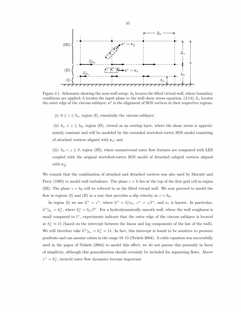
55

h0

h

Δx

Δz

hν

(II)︷

︸︸︷

(III)

︷︸︸

(I)

︷︸︸︷

u|hν

u|h0

ev = ex

ev = eeS

Figure 4.1. Schematic showing the near-wall setup: h0 locates the lifted virtual wall, where boundaryconditions are applied; h locates the input plane to the wall shear stress equation, (4.14); hν locatesthe outer edge of the viscous sublayer; ev is the alignment of SGS vortices in their respective regions.

(i) 0 ≤ z ≤ hν , region (I), essentially the viscous sublayer;

(ii) hν < z ≤ h0, region (II), viewed as an overlap layer, where the shear stress is approxi-

mately constant and will be modeled by the extended stretched-vortex SGS model consisting

of attached vortices aligned with ex; and

(iii) h0 < z ≤ δ, region (III), where nonuniversal outer flow features are computed with LES

coupled with the original stretched-vortex SGS model of detached subgrid vortices aligned

with eeS .

We remark that the combination of attached and detached vortices was also used by Marusic and

Perry (1995) to model wall turbulence. The plane z = h lies at the top of the first grid cell in region

(III). The plane z = h0 will be referred to as the lifted virtual wall. We now proceed to model the

flow in regions (I) and (II) in a way that provides a slip velocity at z = h0.

In region (I) we use u+ = z+, where u+ = u/uτ , z+ = z/l+, and uτ is known. In particular,

u+|hν = h+ν , where h+

ν = hν/l+. For a hydrodynamically smooth wall, where the wall roughness is

small compared to l+, experiments indicate that the outer edge of the viscous sublayer is located

at h+ν ≈ 11 (based on the intercept between the linear and log components of the law of the wall).

We will therefore take u+|hν= h+

ν = 11. In fact, this intercept is found to be sensitive to pressure

gradients and can assume values in the range 10–15 (Nickels 2004). A cubic equation was successfully

used in the paper of Nickels (2004) to model this effect; we do not pursue this presently in favor

of simplicity, although this generalization should certainly be included for separating flows. Above

z+ = h+ν , inviscid outer flow dynamics become important.

56

4.3.4 Slip Velocity at Lifted Virtual Wall

We now model the mean-flow dynamics in region (II), hν < z ≤ h0. We require h0 to scale with

outer flow thickness δ but to remain relatively small, h0 < 0.1 δ, say, so that nonuniversal effects

(the wake) uncharacteristic of the inner scales can be captured by the LES in region (III). This will

permit the LES to be performed with the same grid for a wide range of Re, eliminating the O(Re2τ )

scaling requirement for the grid resolution of a partially resolved wall-bounded LES (Piomelli 2008).

Put another way, h0 remains fixed, O(δ), but hν becomes thinner, O(l+), with increasing Re.

Region (II) is, by construction, the so-called overlap region, or the production-equals-dissipation

layer, where the shear stress is approximately constant. Furthermore, the shear stress is balanced

by the wall shear stress (Townsend 1976). Casting these ideas in LES terminology,

u2τ (x, y, t) = −uw = −uw − Txz = −Txz, since w = 0.

The existence of quasi-streamwise vortical structures in wall turbulence have long been observed

by researchers (e.g., Head and Bandyopadhyay 1981, Robinson 1991), and have also served as useful

physical models (e.g., Bakewell and Lumley 1967, Townsend 1976, Perry and Chong 1982, Marusic

and Perry 1995, Nickels et al. 2007, Adrian 2007). Motivated by these studies, we model region (II)

with an ensemble of vortices aligned in the streamwise direction, (evx, e

vy, e

vz) = (1, 0, 0) ⇔ ev = ex.

Substituting these into the expression for the shear stress produced by the extended stretched-spiral

vortex SGS model, (4.5), and noting that the only nonzero component of the mean velocity gradient

tensor is du/dz, we obtain

Txz = −12γIIK

1/2∆cdudz. (4.16)

Recall the physical mechanism that produces this shear stress: the action of the spiralling streamwise

vortex is to wrap its own axial velocity, now identified as the mean streamwise velocity, as if it were

a passive scalar (see figure 4.2), thereby transporting higher-momentum fluid toward the wall and

transporting low-momentum fluid away from the wall. This process has the observed effect of a

flattened streamwise velocity profile.

Unlike the SGS vortices in region (III), which are unaware of the presence of the wall and

are, therefore, considered as detached from the wall, the size of these near-wall vortices, ∆c, are

constrained by the presence of the wall so that ∆c = z. That is, (4.16) with ∆c → z can be

interpreted as the shear stress produced by a hierarchy of longitudinal vortices that scale with the

wall distance. This scaling assumption is, in fact, the idea of the so-called attached wall eddy (Nickels

et al. 2007). We therefore write (4.16) in the form

dudz

=1K1

uτ

z, (4.17)

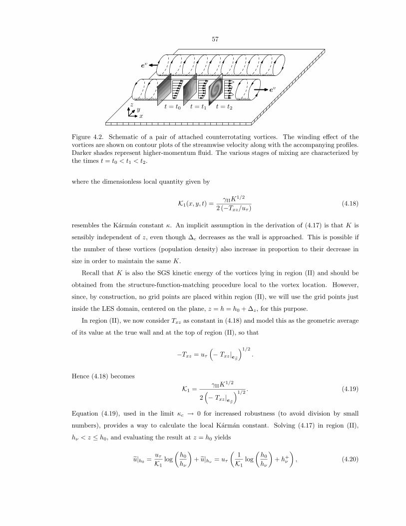
57

xy

z

ev

t = t0 t = t1 t = t2

ev

Figure 4.2. Schematic of a pair of attached counterrotating vortices. The winding effect of thevortices are shown on contour plots of the streamwise velocity along with the accompanying profiles.Darker shades represent higher-momentum fluid. The various stages of mixing are characterized bythe times t = t0 < t1 < t2.

where the dimensionless local quantity given by

K1(x, y, t) =γIIK

1/2

2 (−Txz/uτ )(4.18)

resembles the Karman constant κ. An implicit assumption in the derivation of (4.17) is that K is

sensibly independent of z, even though ∆c decreases as the wall is approached. This is possible if

the number of these vortices (population density) also increase in proportion to their decrease in

size in order to maintain the same K.

Recall that K is also the SGS kinetic energy of the vortices lying in region (II) and should be

obtained from the structure-function-matching procedure local to the vortex location. However,

since, by construction, no grid points are placed within region (II), we will use the grid points just

inside the LES domain, centered on the plane, z = h = h0 + ∆z, for this purpose.

In region (II), we now consider Txz as constant in (4.18) and model this as the geometric average

of its value at the true wall and at the top of region (II), so that

−Txz = uτ

(− Txz|e eS

)1/2

.

Hence (4.18) becomes

K1 =γIIK

1/2

2(− Txz|e eS

)1/2. (4.19)

Equation (4.19), used in the limit κc → 0 for increased robustness (to avoid division by small

numbers), provides a way to calculate the local Karman constant. Solving (4.17) in region (II),

hν < z ≤ h0, and evaluating the result at z = h0 yields

u|h0 =uτ

K1log(h0

hν

)+ u|hν

= uτ

(1K1

log(h0

hν

)+ h+

ν

), (4.20)

58

where the constant of integration has been chosen by putting u|hν = uτ h+ν . We will use (4.20),

which serves as a jump condition between the hν–h0 planes, along with v = 0 and w = 0, to set

the Dirichlet boundary conditions at the lifted virtual wall h0; uτ is obtained from the solution of

(4.15).

Equation (4.20) has been obtained from a physical model of region (II) in which the dominant

Reynolds shear stress is modeled by streamwise-aligned vortices that transport low-momentum mean

streamwise velocity away from the wall and high-momentum mean streamwise velocity toward the

wall. The idea that these self-similar vortices scale only with z—independent of l+ and δ—implies

an overlap argument. Equation (4.20) couples u|h0 with the resolved-scale LES in region (III),

h0 < z ≤ δ, which provides both K and eeS . Equation (4.20) contains two constants, γ and h+ν .

The latter is given empirically by h+ν = 11 from our discussion of region (I); a different value could

be used for rough-wall flows. This physical model provides a means of dynamically calculating the

instantaneous local “Karman constant” K1 as part of the LES. This will be demonstrated later.

It appears from the present construction that we have confined attached eddies to region (II).

This is not the case; the existence of attached eddies in region (II) does not preclude their existence

in region (III). We have only assumed that region (II) is dominated by attached eddies, which led

us to explicitly model their dynamics. If they exist in region (III) and have sizes larger than the

grid spacing, z > ∆x, they would be directly captured by the LES. On the other hand, if they exist

in region (III) and have sizes smaller than the grid spacing, z < ∆x, they would be modeled by the

SGS model.

One may also wonder if these attached eddies still exist near the top of region (II), h0, in very

high Reynolds number flows since we designed h0 to be fixed relative to δ. In the present simulations

h+0 is as high as 149 k. Note, however, that the attached-eddy idea–that they have size z and have

characteristic velocity uτ–is intimately linked with the overlap argument that says that both z and

uτ are the relevant parameters in the overlap region, ν/uτ z δ. In other words, as long as h0/δ

is small, it does not matter how large h+0 is for both z and uτ to emerge as the relevant parameters,

the necessary ingredients for attached eddies.

4.3.5 Estimation of the Mixing Time Constant γII

A constant, γII, is required in (4.20). Owing to the highly anisotropic character of near-wall tur-

bulent physics, this is expected to be somewhat different in value from that used in the SGS scalar

application (Pullin 2000).

Consider the interface of regions (II) and (III), z = h0, where both inner and outer layer modeling

ideas are valid; in the spirit of LES filtering, we interpret this interface as a blurred boundary

between the two regions so that the change in underlying vortical flow is gradual. This interface,

z ≈ h0 < 0.1 δ, is near the wall, so the LES filtered flow field can be approximated by simple shear

59

flow, ∂ui/∂xj = δi1δj3S, where S = du/dz. This implies that, in this region, eeS = (1/√

2, 0, 1/√

2);

that is the detached vortices are inclined at 45 to the wall.

We estimate γII by matching Townsend’s structure parameter,

a1 = T13/Tii = T13/(2K),

of the two vortical flow descriptions at this interface region. Given the vortex alignment, this

parameter measures the amount of shear stress that can be supported relative to the vortex kinetic

energy. First, the eeS alignment and (4.5) give

a1|e eS = (−K|e eS/2)/(2K|e eS ) = −1/4.

Similarly, the ex alignment and (4.5) give

a1|ex = (−γII(K|ex)1/2∆cS/2)/(2K|ex) = −γII∆cS(K|ex)−1/2/4.

To proceed, we assume high Re so that κc → 0. Also, for simplicity, d → 0. The subgrid kinetic

energy of the streamwise vortex then reduces to

K|ex = 2〈(δui)2〉/(π2〈d2〉

).

The local averaging is dominated by the background shear, so we can approximate 〈(δui)2〉 ≈

〈(δu)2〉 ≈ (∆zS)2, and for the same reason 〈d2〉 = (∆z/∆c)2. Then

K|ex = 2 (∆cS/π)2.

Using this, we obtain a1 for the ex aligned vortex,

a1|ex = −2−5/2 π γII.

Finally, matching these, a1|e eS = a1|ex , we have γII = 21/2/π ≈ 0.45. This is the value used presently

for all LES.

4.3.6 Summary of SGS Wall Model

Our SGS model for the near-wall dynamics can be summarized as follows: for every cell adjacent to

both the top and bottom walls, (4.15) is solved for η0 with terms on the right-hand side provided

by the LES at the top of the wall-adjacent cell at z = h = ∆z + h0. This provides η0(x, y, t) and

thus uτ (x, y, t). Equation (4.20) is then used to evaluate the streamwise slip velocity u|h0(x, y, t) at

60

z = h0, with K1 evaluated from (4.19) and with K and Txz|e eS evaluated at z = h = ∆z +h0 from the

LES structure-function-matching procedure. The other boundary conditions at the virtual wall are

taken as v|h0(x, y, t) = w|h0(x, y, t) = 0. This method couples the LES with the modeled, near-wall

dynamics. The LES has implicit knowledge of the true no-slip boundary condition, because this was

used in obtaining (4.15), and the smooth-wall condition through use of h+ν = 11. Because the LES

quantities in both (4.15) and (4.19) are evaluated at the top of the first cell at z = h = ∆z + h0,

the height of the virtual wall at z = h0 should satisfy hν < h0 < h. Presently we use h0 = 0.18 ∆z,

independent of the LES resolution, and consider this as part of the overall grid. Some tests to

investigate sensitivity to h0 were performed.

4.4 Numerical Method

The low-storage third-order semi-implicit Runge–Kutta method of Spalart, Moser and Rogers (1991)

is used for temporal discretization. The implicit treatment of the viscous term allows large time

steps to be taken; in the simulations, the CFL number

∆t max(|u|∆x

,|v|∆y

,|w|∆z

)

was set to unity. The low-storage property simplifies the time step advancement into three sequential

substeps, n = 0, 1, 2, of the same form:

u(n+1)i − u

(n)i

∆t= −(γn + ζn)

∂p(n+1)

∂xi+ γnH

(n)i + ζnH

(n−1)i + αnL

(n)i + βnL

(n+1)i , (4.21a)

∂u(n+1)i

∂xi= 0, (4.21b)

Hi = −12

(∂uiuj

∂xj+ uj

∂ui

∂xj

)− ∂Tij

∂xj+ fi, Li = ν

∂2ui

∂x2j

. (4.21c)

For an arbitrary reference time, t0, u(3)i = ui(t0 +∆t). The value of the constants αn, βn, γn and ζn

are given by Spalart, Moser and Rogers (1991). The discrete pressure p(n+1) is formally a Lagrange

multiplier that enforces (4.21b), including at the boundary.

The governing equations are solved in an Lx × Ly × Lz box with periodic boundary conditions

applied in both the x- and y-directions. Applying the Fourier spectral method for both these

directions results in Nx×Ny sets of one-dimensional complex Helmholtz equations in the z-direction

for each mode (kx, ky), where

kx = 2π/Lx(−Nx/2, . . . ,−1, 0, 1, . . . , Nx/2− 1),

ky = 2π/Ly(−Ny/2, . . . ,−1, 0, 1, . . . , Ny/2− 1).

61

In practice, only half of the Nx × Ny sets of complex equations (or Nx × Ny sets of real equa-

tions, separately counting real and imaginary parts) are solved due to the symmetry of the Fourier

coefficients.

An explicit finite difference scheme with fourth-order global accuracy (third-order boundary,

sixth-order interior) is used to approximate the z derivative on Nz + 1 uniformly spaced nodes,

located at zk = Lz(−1/2 + k/Nz), k = 0, 1, . . . , Nz. When coupled with a certain diagonal norm,

the finite-difference approximation satisfies the summation-by-parts (SBP) property (Strand 1994,

Carpenter, Gottlieb and Abarbanel 1994, Mattsson and Nordstrom 2004). Although stability in

the sense described in those papers is not preserved because Dirichlet boundary conditions are

applied directly (injection method), our experience indicates that stability is not an issue, at least

presently, where the diffusion operator is advanced implicitly. In explicit schemes, a seven-point

stencil is required to achieve sixth-order accuracy, but, following Hill and Pullin (2004), we use two

additional points to minimize the Ghosal truncation error (Ghosal 1996). The Ghosal truncation

error pertains to errors resulting from the application of spatial discretization schemes to the Navier–

Stokes equations. Unsurprisingly, in reducing the Ghosal truncation error, the high-wavenumber

performance of the finite-difference scheme is also simultaneously improved (Hill and Pullin 2004).

Such a scheme, called a tuned centered-difference (TCD) method by Hill and Pullin (2004), is also

combined with the SBP scheme in Pantano et al. (2007). Complete details of the Nz + 1×Nz + 1

finite-difference matrix Dz are provided in § 4.4.1.

Spatially discretizing (4.21), we obtain for each mode (kx, ky) and node zk:

(D2

z − λ2)u = ikxζ

′p+R1 + σ1,(D2

z − λ2)v = ikyζ

′p+R2 + σ2,(D2

z − λ2)w = Dzζ

′p+R3 + σ3,

(4.22a)

ikxu+ iky v +Dzw = 0, (4.22b)

where λ2 = k2x+k2

y+1/(βν∆t) and ζ ′ = (γ+ζ)/(βν). The spatial discretization of (u, p)(n+1)(x, y, z)

is denoted (u, p)(kx, ky, k). For clarity, we have dropped the superscript and subscript n from (4.21);

Ri are known terms, obtained by simple rearrangement; σi are incurred penalty terms for directly

imposing Dirichlet boundary conditions on the velocity at k = 0 and k = Nz (or equivalently, at

z = ±Lz/2),

(u, v, w)(kx, ky, 0) = (g1−, g2

−, g3−)(kx, ky),

(u, v, w)(kx, ky, Nz) = (g1+, g2

+, g3+)(kx, ky).

(4.23)

In other words, because we choose to satisfy (4.23), (4.22) written without σi cannot be satis-

fied at k = 0 and k = Nz. Although we call σi a penalty term, it should not be confused with

the simultaneous-approximation-term (SAT) technique (Carpenter, Gottlieb and Abarbanel 1994),

62

where σi is explicitly specified. Here, σi must be determined as part of the solution procedure. Note,

however, that the divergence constraint, (4.22 b), is satisfied everywhere, even at the boundaries,

k = 0 and k = Nz.

The discrete pressure Poisson equation is obtained by applying the discrete divergence to the

momentum equations:

(D2

z −[k2

x + k2y

])ζ ′p = −Rp − (ikxσ1 + ikyσ2 +Dzσ3) , (4.24)

where Rp = ikxR1 + ikyR2 + DzR3. In general, Dzσ3 is nonzero in the interior of the domain,

k = 1, 2, . . . , Nz−1. That is σi, appearing only at the boundaries of (4.22 a) carry over as additional

interior source terms to (4.24). Careful accounting of the σi terms is key to ensuring discrete mass

conservation up to machine precision. Unlike in well-resolved simulations such as DNS in which σi

is small and can thus be safely ignored, σi in LES is large and if ignored will be a source of nonzero

velocity divergence that leads to numerical instability (Canuto et al. 1987). The method for solving

this coupled problem in the discrete framework is the Kleiser–Schumann influence-matrix method,

detailed by Canuto et al. (1987). Although they presented it for the Chebyshev-tau and spectral

collocation discretizations with homogeneous boundary conditions, the method is quite general, and

we extend its usage here for finite differences with nonhomogeneous boundary conditions.

As written, the nonlinear products in (4.21 c) are computed in skew-symmetric form in physical

space. Then, Hi, which includes the nonlinear products and the LES contributions, is transformed

to wavenumber space, where a p1th-order Fourier exponential filter (Gottlieb and Shu 1997, Hou

and Li 2007) of the form

σ(ξ) = exp(−α1ξp1) (4.25)

is applied in the periodic directions, ξ = |kx|/(π/∆x), |ky|/(π/∆y); p1 = 36; α1 is chosen so that

σ(2/3) = 1/2. The high-order filter, with flat response at resolved wavenumbers and sharp but

smooth drop at the cutoff wavenumber, mimics the 2/3-dealiasing rule. In an LES employing a local

physical-space SGS model, the filter’s smooth cutoff minimizes Gibbs oscillations that, posing as

steep local gradients, would artificially activate the SGS model.

The set of ODEs, (4.15) for the wall shear stress, τ0(x, y, t) = νη0(x, y, t), are advanced using

the same third-order Runge–Kutta scheme as the main part of the flow simulation. The overall

computing overhead for the implementation of the stretched-vortex SGS model is less than 10% of

the overall computing time. Because the numerical solution of the wall ODE set occurs only in

boundary cells, this constitutes a small part of the SGS-related computing effort.

63

4.4.1 SBP TCD Derivative Matrix

We provide details of the fourth-order globally accurate explicit finite-difference Nz + 1 × Nz + 1

matrix, Dz. This matrix operates on any Nz + 1 vector, u, say, whose elements uk represent nodal

discretizations of the continuous function u(z) at uniformly spaced nodes, zk = −Lz/2 + k∆z,

∆z = Lz/Nz k = 0, 1, . . . , Nz, such that u(zk) = uk. SBP operators (Strand 1994, Mattsson and

Nordstrom 2004) are constructed from the following decomposition:

Dz =1

∆zH−1Q, Q+QT = B, B = diag(−1, 0, . . . , 0, 1); (4.26a,b,c)

H = HT > 0 and is used to define an inner product, (u, u)H = uTHu, which, in turn, defines a

norm on u, given by ||u||2H = (u, u)H . Although many possible choices for such H exist, we will only

consider the diagonal norm,

H = diag(h0, h1, . . . , hNz ), (4.27)

which restricts the order of accuracy of the boundary scheme to at most half the order of accuracy

of the interior scheme (Strand 1994). Although not pursued presently, an SBP scheme with diagonal

norm can be easily generalized to apply on arbitrarily mapped grids by absorbing the scaling factors

into H. Presently, a third-order boundary scheme coupled with a sixth-order interior scheme, equiv-

alent to a fourth-order global scheme, is chosen. The boundary scheme covers the finite-difference

approximation for the first and last six points, k = 0, 1, . . . , 5, Nz − 5, Nz − 4, . . . , Nz, while the

interior scheme covers the rest, k = 6, 7, . . . , Nz − 6.

The sixth-order TCD (Hill and Pullin 2004), which has a wider nine-point stencil, is used as

the interior scheme. The extra degree of freedom is used to improve spectral resolution by reducing

truncation errors inherent in the Navier–Stokes equations. Any nine-point sixth-order centered

difference approximation for the derivative is given by

Dzuk =1

∆z

4∑j=0

dj (uk+j − uk−j) , (4.28)

where d0 = 0; d1 = 3/4− 14d4; d2 = −3/20 + 14d4; d3 = 1/60− 6d4; and d4 is the free parameter.

Setting d4 = 0 recovers the standard sixth-order explicit scheme; setting d4 = −1/280 recovers the

standard eighth-order explicit scheme; d4 is determined by minimizing the Ghosal truncation error

(Ghosal 1996), a procedure detailed by Hill and Pullin (2004). Here, we only give the final result:

d4 = −0.0166.

Comparing (4.26a), (4.27) and (4.28), we identify the TCD scheme in the context of the SBP

64

operator as

hk = 1, Qkj =

dj−k, 0 ≤ j − k ≤ 4,

−dk−j , 0 < k − j ≤ 4,

0, otherwise,

(4.29a,b)

for k = 6, 7, . . . , Nz − 6.

To determine the boundary scheme, write (4.26a) and (4.27) explicitly for k = 0, 1, . . . , 5:

hk(∆z)(Dzu)k =10∑

j=0

Qkjuj =5∑

j=0

Qkjuj +10∑

j=6

Qkjuj . (4.30)

The second term on the right-hand side is known from using (4.26b) and (4.29):

Qkj = −Qjk = −(−dj−k) = dj−k

for k = 0, 1, . . . , 5, j = 6, 7, . . . , 10, 0 < j − k ≤ 4. Substituting this in (4.30) gives

hk(∆z)(Dzu)k =5∑

j=0

Qkjuj +k+4∑j=6

dj−kuj . (4.31)

The remaining unknowns to be solved are the 6×6 block, Qkj (k, j = 0, 1, . . . , 5) and the six-element

vector hk (k = 0, 1, . . . , 5). For each k, match the coefficients from the series expansion of (4.31) up

to (∆z)3 and apply (4.26b) to determine the remaining unknowns up to a another free parameter,

Q45, say, different from d4 (see Strand 1994). We choose Q45 by minimizing the so-called average

boundary truncation error (Diener et al. 2007), giving Q45 = (17 171− 329 670d4)/24 300.

4.4.2 Code Validation

To validate our code, we reproduced the Reτ = 180 DNS of Kim, Moin and Moser (1987) using

Lx × Ly × Lz = 2πδ × 4πδ/3 × 2δ and Nx × Ny × Nz = 192 × 192 × 192. The main difference

between these two codes is the discretization scheme in the wall-normal direction: Kim, Moin and

Moser (1987) used a Chebyshev-tau scheme on a stretched–cosine grid, while we used a fourth-order

finite-difference scheme on a uniformly spaced grid. The statistics from the present code are taken

at a snapshot in time. As seen in figures 4.3 and 4.4, these are in good agreement with Kim, Moin

and Moser (1987).

65

0

5

10

15

20

100 101 102 103

z+

u+

Figure 4.3. Mean velocity profile from Reτ = 180 DNS: , present code; , Kim, Moin andMoser (1987).

0.0

1.0

2.0

3.0

4.0

0.0 0.2 0.4 0.6 0.8 1.0

(a)

0.0

0.5

1.0

1.5

2.0

0.0 0.2 0.4 0.6 0.8 1.0

(b)

0.0

0.5

1.0

1.5

0.0 0.2 0.4 0.6 0.8 1.0

z/δ

(c)

0.0

0.5

1.0

1.5

0.0 0.2 0.4 0.6 0.8 1.0

z/δ

(d)

Figure 4.4. Turbulence statistics, (a) u+rms, (b) v+

rms, (c) w+rms and (d) −uw+ from Reτ = 180 DNS:

, present code; , Kim, Moin and Moser (1987).

66

Table 4.1. LES parameters and outputs for turbulent channel flow.

Case Rec Reτ η(%) Lx/δ′ Ly/δ′ h0/∆z Nx Ny Nz ∆+x γIII K1

A1 49 k 2 k 1.1 32 8 0.18 192 48 48 3.3× 102 0 0.37A2 610 k 20 k 2.2 32 8 0.18 192 48 48 3.3× 103 0 0.38A3 7400 k 200 k 2.9 32 8 0.18 192 48 48 3.3× 104 0 0.38A4 87 M 2 M 2.1 32 8 0.18 192 48 48 3.3× 105 0 0.37A5 990 M 20 M 1.7 32 8 0.18 192 48 48 3.3× 106 0 0.37

B2 610 k 20 k 2.9 32 8 0.18 384 96 96 1.7× 103 0 0.38B3 7400 k 200 k 2.7 32 8 0.18 384 96 96 1.7× 104 0 0.38B4 86 M 2 M 2.2 32 8 0.18 384 96 96 1.7× 105 0 0.38

C2 580 k 20 k 3.6 32 8 0.18 192 48 48 3.3× 103 0.45 0.39C3 6900 k 200 k 1.0 32 8 0.18 192 48 48 3.3× 104 0.45 0.40C4 81 M 2 M −0.4 32 8 0.18 192 48 48 3.3× 105 0.45 0.39

F2 620 k 20 k −0.8 32 8 0.36 192 48 48 3.3× 103 0 0.38F3 7600 k 200 k 0.6 32 8 0.36 192 48 48 3.3× 104 0 0.38F4 89 M 2 M 0.8 32 8 0.36 192 48 48 3.3× 105 0 0.38

4.5 Results and Discussion

The LES presently performed are summarized in table 4.1: k ≡ 103,M ≡ 106; Rec ≡ ucδ/ν; uc

is the mean centerline velocity; Reτ ≡ uτδ/ν; η ≡ (Reτ )act/Reτ − 1; δ′ ≡ Lz/2 = δ − h0 ≈ δ;

∆x = ∆y = 4∆z; Reτ is nominal, (Reτ )act is actual; and γIII refers to γ in (4.5) used in the interior

of the LES domain. Four sets were done and are labeled A, B, C and D. All used the same form of

the wall SGS model with γII = 0.45. For sets A and B, the original form of the stretched-vortex SGS

model was used in region (III). This corresponds to γIII = 0 in (4.5). For set C, γIII = 0.45 was used

in (4.5). There is no inconsistency with γII 6= γIII: the former is a necessary part of the special SGS

model in region (II), while the latter forms part of the global SGS model for LES in region (III). Set

F is used to evaluate the wall model’s sensitivity to the virtual wall location h0. The simulations

are run until the first- and second-order statistics have converged. Data is then collected from one

snapshot in time; our interest is in low-order statistics, which do not benefit significantly from time

averaging.

4.5.1 Profiles

The mean streamwise velocity profiles for Reτ = 2k–20 M (set A) corresponding to the original LES

model (γIII = 0) coupled with the present wall model are shown in figure 4.5, where ( ) denotes the

xy-plane average at a particular time. Also shown is the log relationship (4.20) with the predicted

K1 averaged across all cases, (K1)avg = 0.37. Its intercept is 11− log(11)/0.37 = 4.5 (compare with

the classic value of ∼ 5). The slight drop in the mean-flow profile for the two points adjacent to

67

0

10

20

30

40

50

60

100 101 102 103 104 105 106 107 108

z+

u+

Figure 4.5. Mean velocity profiles for LES with γIII = 0 (set A): , Reτ = 2 k; , Reτ = 20 k; ,Reτ = 200 k; 4 , Reτ = 2M; ∇ , Reτ = 20M; , Reτ = 2k DNS (Hoyas and Jimenez 2006);

, log(z+/11)/0.37 + 11.

the lifted virtual wall was thought to be a manifestation of a spurious sublayer due to the Dirichlet

slip and no-transpiration boundary conditions (Cabot and Moin 1999). This issue is not specific

to Dirichlet boundary conditions but can also be observed in wall stress boundary conditions (see

Pantano et al. 2008). The flow quickly recovers beyond the two points and appears to follow the log

profile.

We plot the corresponding profiles of the turbulent statistics in figure 4.6, where ( )rms refers to

the root mean square (r.m.s.) of the fluctuations. The mild near-wall oscillations may suggest that

we used an inadequate time-averaging interval. However, the localized nature of these oscillations

and similar observations by Pantano et al. (2008) offer the explanation that they are, in fact, Gibbs

oscillations caused by the singular no-penetration boundary condition.

Recently, the peak in near-wall u-fluctuations was observed to be mildly increasing with Reynolds

number (DeGraaff and Eaton 2000, Del Alamo et al. 2004). This peak, located at z+ ≈ 12, is

beneath our lifted wall, z = h0, and well within our modeled near-wall layer consisting of streamwise

vortices—region (II). Accordingly, we do not expect to capture this trend with statistics of the

present simulations, which are essentially an outer-layer—region (III)—LES. This is a limitation of

the present wall model.

The w-fluctuations are uniformly underpredicted; this is not surprising, since we used the no-

transpiration boundary condition, which does not strictly hold at the lifted virtual wall. This

amounts to letting the LES SGS model predict all near-wall w-fluctuations, as confirmed by the

subgrid component in figure 4.6(c). The overall anisotropy in the Reynolds stresses, however, is

preserved by our anisotropic LES model, even close to the wall. Physically, we are letting the LES

68

0.0

1.0

2.0

3.0

4.0

0.0 0.2 0.4 0.6 0.8 1.0

(a)

0.0

0.5

1.0

1.5

2.0

0.0 0.2 0.4 0.6 0.8 1.0

(b)

0.0

0.5

1.0

1.5

0.0 0.2 0.4 0.6 0.8 1.0

z/δ

(c)

0.0

0.5

1.0

1.5

0.0 0.2 0.4 0.6 0.8 1.0

z/δ

(d)

Figure 4.6. Turbulence statistics, (a) u+rms, (b) v+

rms, (c) w+rms and (d) −uw+, for LES with

γIII = 0 (set A): , Reτ = 2 k; , Reτ = 20 k; , Reτ = 200 k; 4 , Reτ = 2 M; ∇ , Reτ = 20 M;, Reτ = 2k DNS (Hoyas and Jimenez 2006); open symbols, total (resolved plus subgrid); solid

symbols, subgrid.

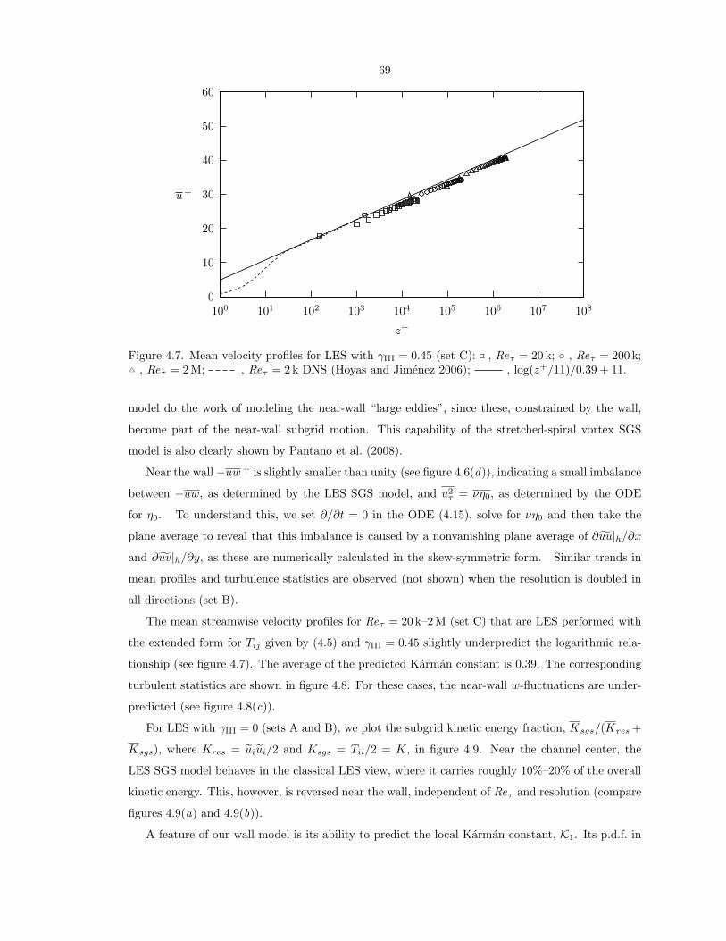
69

0

10

20

30

40

50

60

100 101 102 103 104 105 106 107 108

z+

u+

Figure 4.7. Mean velocity profiles for LES with γIII = 0.45 (set C): , Reτ = 20 k; , Reτ = 200 k;4 , Reτ = 2M; , Reτ = 2k DNS (Hoyas and Jimenez 2006); , log(z+/11)/0.39 + 11.

model do the work of modeling the near-wall “large eddies”, since these, constrained by the wall,

become part of the near-wall subgrid motion. This capability of the stretched-spiral vortex SGS

model is also clearly shown by Pantano et al. (2008).

Near the wall −uw+ is slightly smaller than unity (see figure 4.6(d)), indicating a small imbalance

between −uw, as determined by the LES SGS model, and u2τ = νη0, as determined by the ODE

for η0. To understand this, we set ∂/∂t = 0 in the ODE (4.15), solve for νη0 and then take the

plane average to reveal that this imbalance is caused by a nonvanishing plane average of ∂uu|h/∂x

and ∂uv|h/∂y, as these are numerically calculated in the skew-symmetric form. Similar trends in

mean profiles and turbulence statistics are observed (not shown) when the resolution is doubled in

all directions (set B).

The mean streamwise velocity profiles for Reτ = 20 k–2M (set C) that are LES performed with

the extended form for Tij given by (4.5) and γIII = 0.45 slightly underpredict the logarithmic rela-

tionship (see figure 4.7). The average of the predicted Karman constant is 0.39. The corresponding

turbulent statistics are shown in figure 4.8. For these cases, the near-wall w-fluctuations are under-

predicted (see figure 4.8(c)).

For LES with γIII = 0 (sets A and B), we plot the subgrid kinetic energy fraction, Ksgs/(Kres +

Ksgs), where Kres = uiui/2 and Ksgs = Tii/2 = K, in figure 4.9. Near the channel center, the

LES SGS model behaves in the classical LES view, where it carries roughly 10%–20% of the overall

kinetic energy. This, however, is reversed near the wall, independent of Reτ and resolution (compare

figures 4.9(a) and 4.9(b)).

A feature of our wall model is its ability to predict the local Karman constant, K1. Its p.d.f. in

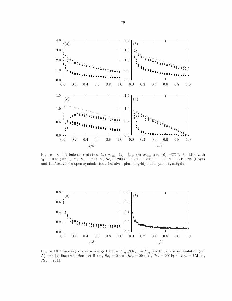
70

0.0

1.0

2.0

3.0

4.0

0.0 0.2 0.4 0.6 0.8 1.0

(a)

0.0

0.5

1.0

1.5

2.0

0.0 0.2 0.4 0.6 0.8 1.0

(b)

0.0

0.5

1.0

1.5

0.0 0.2 0.4 0.6 0.8 1.0

z/δ

(c)

0.0

0.5

1.0

1.5

0.0 0.2 0.4 0.6 0.8 1.0

z/δ

(d)

Figure 4.8. Turbulence statistics, (a) u+rms, (b) v+

rms, (c) w+rms and (d) −uw+, for LES with

γIII = 0.45 (set C): , Reτ = 20 k; , Reτ = 200 k; 4 , Reτ = 2 M; , Reτ = 2 k DNS (Hoyasand Jimenez 2006); open symbols, total (resolved plus subgrid); solid symbols, subgrid.

0.0

0.2

0.4

0.6

0.8

0.0 0.2 0.4 0.6 0.8 1.0

z/δ

(a)

0.0

0.2

0.4

0.6

0.8

0.0 0.2 0.4 0.6 0.8 1.0

z/δ

(b)

Figure 4.9. The subgrid kinetic energy fraction Ksgs/(Kres +Ksgs) with (a) coarse resolution (setA), and (b) fine resolution (set B): , Reτ = 2k; , Reτ = 20 k; , Reτ = 200 k; 4 , Reτ = 2M; ∇ ,Reτ = 20M.

71

0

30

60

90

0.30 0.35 0.40 0.45 0.50

K1

(a)

0

10

20

30

0.30 0.35 0.40 0.45 0.50

K1

(b)

Figure 4.10. P.d.f.s of the predicted Karman constant, K1, for LES with (a) γIII = 0 (set A),(K1)avg = 0.37 and (b) γIII = 0.45 (set C), (K1)avg = 0.39: , Reτ = 2 k; , Reτ = 20 k; ,Reτ = 200 k; 4 , Reτ = 2M; ∇ , Reτ = 20M.

figure 4.10 shows peak values around 0.38, with a wider distribution for the cases with γIII = 0.45.

The notion of variable K1 was also suggested by Nickels (2004), who found that K1 could also be

sensitive to pressure gradients. This is consistent with the present modeling approach, where all local

wall-adjacent cells are subjected to outer flow forcing with pressure gradients and should therefore

have their own K1, although their average K1 should agree with experiments or DNS data.

Figure 4.11 shows that the mean velocity profiles are not very sensitive to a doubling of the

virtual wall location, h0, from h0 = 0.18 ∆z to h0 = 0.36 ∆z, We found some sensitivity when h0

was decreased below 0.1 ∆z and this is not recommended. With ζ0 ≡ h0/∆z and ∆z = Lz/Nz,

δ = Lz/2+h0, we have, in inner variables, h+0 = 2ζ0Reτ/(Nz +2ζ0). We require that h+

0 > h+ν = 11.

This is satisfied always presently. We note that for Reτ = 2k, this is not satisfied with N = 96, and

these runs were done only with N = 48 for which h+0 ≈ 15 with ζ0 = 0.18.

4.5.2 Resolved-Scale Spectra

The one-dimensional power spectra of streamwise velocity fluctuations, Euu, at the quarter-channel

height z/δ = 0.5 is shown in figure 4.12. We adopt the following convention

u2rms =

∫ ∞

0

Euu(kx) dkx =∫ ∞

0

Euu(ky) dky.

The plots are normalized with the plane-averaged Kolmogorov scales ε and ν, where the total

dissipation ε = εres + εsgs, the resolved dissipation εres = 2νSijSij and the subgrid dissipation

εsgs =∫∞

kc2νk2E(k) dk. For reference, Ksgs/(Kres +Ksgs) . 0.2 at this wall-normal plane (figure

4.9(a)). Also in figure 4.12 are model spectra (Pope 2000, figure 6.14) that fit data from nearly

two decades (30–1500) of Taylor-scale Reynolds numbers, as compiled by Saddoughi and Veeravalli

(1994). To reproduce the model spectra of Pope (2000), we use the parameters ε, ν and the isotropic

72

0

10

20

30

40

50

60

70

101 102 103 104 105 106 107 108

z+

u+

h0/Δz = 0.18

h0/Δz = 0.36

Figure 4.11. Model sensitivity to virtual wall location, h0: upper set (set F), (K1)avg = 0.38, shiftedup by 10 units for clarity; lower set (set A), (K1)avg = 0.37; , Reτ = 20 k; , Reτ = 200 k; 4 ,Reτ = 2M; , log(z+/11)/(K1)avg + 11.

10−2

100

102

104

106

108

1010

10−7 10−6 10−5 10−4 10−3 10−2 10−1 100 101

Eu

u/(

εν5)1

/4

kx(ν3/ε)1/4

Figure 4.12. Resolved spectra at z/δ = 0.5 for set A: , Reτ = 2k; , Reτ = 20 k; , Reτ = 200 k;4 , Reτ = 2M; ∇ , Reτ = 20M; , model spectra (Pope 2000).

73

surrogate for the turbulent kinetic energy, 3u2rms/2, where u2

rms = uu+T xx. The envelope produced

by the composite of all the spectra collapses onto the same k−5/3 line, suggesting that in all cases,

the Kolmogorov scale—and hence the total dissipation—are accurately predicted by the LES model,

independent of Reτ . The rapid (∼ 6 points) drop near the 2/3-cutoff wavenumber is purely an artifact

of the exponential smoothing, (4.25). The rest of the drop could be attributed to dominant SGS

dynamics that overwhelm the resolved scales in that wavenumber range, resulting in the observed

effect of excess resolved wavenumbers. To test this idea, we need the subgrid extension of the

spectrum representing the dynamics of the SGS model.

4.5.3 Subgrid-Continued Spectra

A benefit of the stretched-spiral vortex model for LES is the availability of a closed-form spectral

representation of the local Navier–Stokes solution that can be used to obtain the subgrid-continued

spectra down to Kolmogorov scales. This was demonstrated for both velocity and scalar spectra by

Hill, Pantano and Pullin (2006).

Given that the SGS vortices are oriented according to the delta-function distribution (§ 4.2.2),

the one-dimensional spectrum tensors derived by Pullin and Saffman (1994) (equations (49)–(51))

for an ensemble of cylindrical vortices reduce to

Θ11(k3) =2π

∫ ∞

|k3/ sin θ|E(k)

(k2 − k2

3

sin2 θ

)−1/2

×[

1k2

cos2 θ cos2 φ(k2 − k2

3

sin2 θ

)+

1k2

sin2 φk23

sin2 θ

]1

sin θdk, (4.32a)

Θ22(k3) =2π

∫ ∞

|k3/ sin θ|E(k)

(k2 − k2

3

sin2 θ

)−1/2

×[

1k2

cos2 θ sin2 φ

(k2 − k2

3

sin2 θ

)+

1k2

cos2 φk23

sin2 θ

]1

sin θdk, (4.32b)

Θ33(k3) =2π

∫ ∞

|k3/ sin θ|E(k)

(k2 − k2

3

sin2 θ

)−1/2

×[

1k2

sin2 θ

(k2 − k2

3

sin2 θ

)]1

sin θdk, (4.32c)

with E(k) is given by (4.3). Here, the Euler angles θ and φ (the delta-function peak locations) are

defined relative to the (x1, x2, x3) coordinate system, which is not necessarily coincident with the

laboratory frame (different from § 4.2.2). The even function Θii(k3), no summation over i, is defined

such that∫∞−∞ Θii(k3) dk3 = (ui)2rms, from which it follows that Eii(k3) = 2Θii(k3). To obtain the

subgrid-continued Eii(kx), we choose k3 to coincide with kx; that is θ is the angle between the vortex

axis and the x-axis. Given the wavenumber kx, Eii(kx) is found by averaging (4.32) over every cell

on the xy-plane; Eii(ky) is obtained in a similar manner. We remark that this calculation requires

74

10−2

100

102

104

106

10−5 10−3 10−1 101

kx(ν3/ε)1/4

(a)

10−2

100

102

104

106

10−5 10−3 10−1 101

ky(ν3/ε)1/4

(b)

Figure 4.13. Effect of grid resolution on (a) Euu(kx)/(εν5)1/4, and (b) Euu(ky)/(εν5)1/4 at z/δ = 0.5for Reτ = 20 k: case A2; case B2; open symbols, resolved; solid symbols, subgrid.

only numerical information obtained from the LES through E(k); no additional tuning parameters

are required. Also, this calculation is only performed when subgrid-continued spectra are required;

it is not a required part of the resolved-scale LES simulation.

Figure 4.13 shows both resolved and subgrid contributions to Euu(kx) and Euu(ky) for the

Reτ = 20 k case with two different grid resolutions. As the resolution is increased, the resolved

spectra extend themselves to higher wavenumbers, following their subgrid extensions. Note, however,

that the subgrid extensions remain unchanged as the resolution is increased; on this basis, one could

claim that the SGS dynamics have converged. Unlike Euu(kx), Euu(ky) appears not to suffer from

excess resolution, dropping sharply only near the 2/3-cutoff wavenumber. The subgrid part of

Euu(kx) (see figure 4.13(a)) continues where the resolved part drops off, reinforcing the idea that

the SGS dynamics effectively take over.

We compare our LES prediction of Euu at various wall distances with the DNS data of Hoyas

and Jimenez (2006) in figure 4.14. The z/δ = 0.2 plane corresponds to our fifth off-wall grid point,

where Ksgs/(Kres +Ksgs) ≈ 0.2 (see figure 4.9(a)). At these wall locations, the composite of the

resolved and subgrid components appear to faithfully capture the main features of the DNS spectra.

These features include the spatial anisotropy of the subgrid extensions, seen in the ordering of the

subgrid Euu(kx) and Euu(ky), and the hump in the resolved Euu(ky) in the range 10−3 < k+y < 10−2,

which becomes less prominent as z/δ increases from 0.2 to 1. In figure 4.14(a), the subgrid extension

of Euu(kx) is slightly steeper than the DNS result. This may be due to a mismatch between the

near-wall physics, which, perhaps, is exhibiting a k−1 range (Perry and Chong 1982), and our LES

model based on stretched-spiral vortices, which have an inherent k−5/3 inertial range.

We also plot one-dimensional spectra for the spanwise and wall-normal velocity components at

z/δ = 0.5 in figure 4.15. Comparing the spectra for the three velocities at the same wall-normal

location (figures 4.15(a, b) and 4.14(b)), we see a faithful reproduction of the velocity anisotropy, as

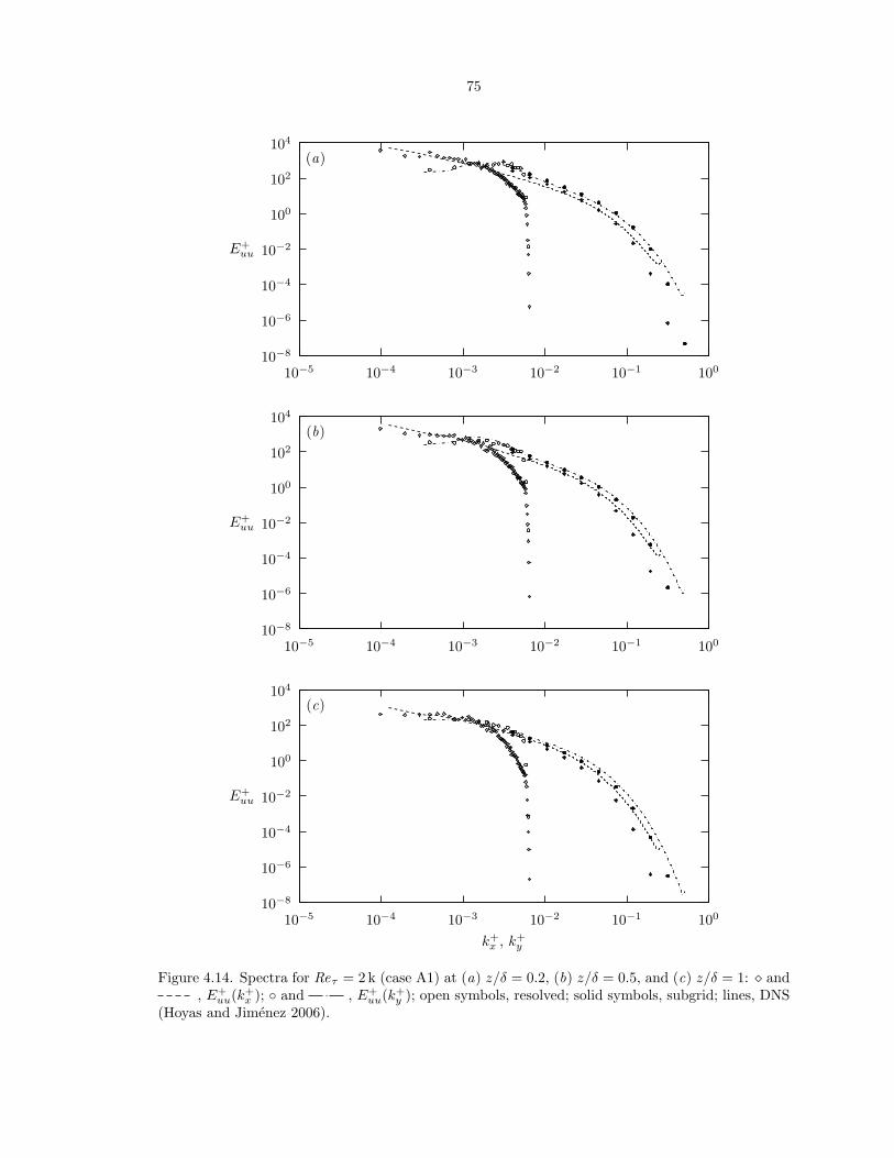
75

10−8

10−6

10−4

10−2

100

102

104

10−5 10−4 10−3 10−2 10−1 100

E+uu

(a)

10−8

10−6

10−4

10−2

100

102

104

10−5 10−4 10−3 10−2 10−1 100

E+uu

(b)

10−8

10−6

10−4

10−2

100

102

104

10−5 10−4 10−3 10−2 10−1 100

k+x , k+

y

E+uu

(c)

Figure 4.14. Spectra for Reτ = 2k (case A1) at (a) z/δ = 0.2, (b) z/δ = 0.5, and (c) z/δ = 1: and, E+

uu(k+x ); and , E+

uu(k+y ); open symbols, resolved; solid symbols, subgrid; lines, DNS

(Hoyas and Jimenez 2006).

76

10−8

10−6

10−4

10−2

100

102

104

10−5 10−4 10−3 10−2 10−1 100

E+vv

(a)

10−8

10−6

10−4

10−2

100

102

104

10−5 10−4 10−3 10−2 10−1 100

k+x , k+

y

E+ww

(b)

Figure 4.15. Spectra for Reτ = 2 k (case A1) at z/δ = 0.5: and , E+vv(k+

x ) and E+ww(k+

x ); and , E+

vv(k+y ) and E+

ww(k+y ); open symbols, resolved; solid symbols, subgrid; lines, DNS

(Hoyas and Jimenez 2006).

77

well as the spatial anisotropy, both in the resolved components and the subgrid extension; in fact,

the ordering of the subgrid Euu(kx) and Euu(ky) is switched for the subgrid Evv(kx) and Evv(ky)

in 10−2 < k+x , k

+y < 10−1.

4.5.4 Wall Model in Inhomogeneous Flows

Since the present near-wall model is entirely local, it can readily be applied to inhomogeneous

turbulent flows. While the predictive performance of a wall model in complex turbulent flows,

especially those involving separation, can only be validated with an a posteriori analysis and further

LES, some prior analysis may guide our expectations of the present model, which we now discuss.

First, we have argued that our approach is not an equilibrium model in the sense of Piomelli

(2008). Presently the local–inner-scaling assumption (4.11) is used in a local sense to reduce only the

unsteady term in the plane-filtered, wall-normal-averaged, streamwise momentum equation, leading

to (4.15). We stress again that in this reduction, a specific F (z+) is not required. Further, our

log-like profile (4.20) does not use (4.11) but is derived directly from the stretched-vortex subgrid

model combined with the attached eddy hypothesis in a way that couples with the resolved-scale

LES. In fact, the effective and local “Karman constant” (4.19) depends partially on LES-derived

quantities and so is also a mixed inner–outer scale parameter. Thus the combination of (4.15) and

(4.20) can be viewed as containing elements of both restricted inner scaling and the outer flow via

the LES. The overall model is therefore only partially reliant on inner scaling. This may be an

improvement over TBLE approaches, where the log law is implied by the damped mixing-length

eddy viscosity. We note that even when this log law is assumed, the TBLE approach improves the

prediction of separated flows relative to equilibrium log law models (Cabot and Moin 1999).

Second, we can show that (4.15) contains an inherent signature for incipient separation in the

sense that uτ (x, y, t) vanishes locally. At each wall-adjacent (x, y) location, (4.15) can be written in

the form (η0 ≡ ∂u/∂z|0)dη0dt

= Λη0(η0 − η0), (4.33)

where

Λ(t) =2νh u|h

, η0(t) = −1νuw|h −

h

ν

(∂uu|h∂x

+∂uv|h∂y

+∂p

∂x

∣∣∣∣h

)+∂u

∂z

∣∣∣∣h

. (4.34a,b)

After using the integrating factor,

I(t) = exp(−∫ t

0

Λ(s)η0(s) ds), (4.35)

78

(4.33) becomes separable, and its exact solution, written as an integral, is

1η0(t)

=I(t)η0(0)

+ I(t)∫ t

0

Λ(s)I(s)

ds, (4.36)

For simplicity now assume constant coefficients η0(t) = η0(0) and Λ(t) = Λ(0); then

1η0(t)

=1

η0(0)e−tΛ(0)eη0(0) +

1η0(0)

(1− e−tΛ(0)eη0(0)

),

so that η0(t) ∼ η0(0) for t 1/[Λ(0)η0(0)]. Roughly, this means η0 tends toward the steady state

η0 at the rate Λη0. A separation criterion can now be obtained based on (4.36). Without loss of

generality, assume that η0(t = 0) > 0. Separation, defined by η0 = 0, would occur at t = ts > 0.

We know I(ts) > 0 from (4.35), and upon assuming that I(ts) < ∞, we require the integral in

(4.36) to be singular for separation. A sufficient condition is Λ(t) = O(t− ts)−1 to give a logarithmic

singularity. From the definition of Λ(t) in (4.34 a), we require that u|h = O(t − ts). When t > ts,

u|h changes sign, indicating that the outer flow has separated and is now reversed.

When the lifted wall penetrates the outer edge of the viscous sublayer, h+0 < h+

ν = 11, which

occurs near separation or in a laminar flow, the logarithmic boundary condition (4.20) would be

replaced with the linear relationship u+|h0 = h0+.

Finally, in the interests of minimizing discretization errors, we tested the present model on

a purpose-built high-accuracy research code. However, we expect similar model performance on

general-purpose codes—see Pantano et al. (2008), who successfully employed a second-order code to

run a similar LES SGS model coupled with a different wall model.

79

Chapter 5

LES of Long Channel Flows

5.1 Background

Recently, Monty et al. (2007), Hutchins and Marusic (2007a,b), Mathis, Hutchins and Marusic (2009)

observed long meandering structures in the log layer of boundary layers, channels, and pipes. These

structures are marked by streamwise-oriented alternating low- and high-momentum streaks, and

have lengths ranging from 6δ to 25δ (δ is the boundary layer thickness, channel half width, or pipe

diameter). The relative energy content of these structures can be observed when plotting contours

of the premultiplied longitudinal energy spectra, kxEuu(kx, z), on the log(λx)–log(z) plane, where

λx = 2π/kx; Hutchins and Marusic (2007b) found that the long structures were related to the peak

found at (z/δ, λx/δ) = (0.06, 6) for Reτ = 7.3 k. Mathis, Hutchins and Marusic (2009) later found

that the wall-normal location of this peak to scale with the middle of the log layer z+ =√

15Re1/2τ ,

or equivalently, z/δ =√

15Re−1/2τ .

According to Mathis, Hutchins and Marusic (2009), these large-scale structures are responsible

for modulating the amplitudes of superimposed small-scale fluctuations. To test this idea, they

extracted the large-scale signal by low-pass filtering the streamwise velocity at λx/δ > 1, and then

computed the correlation coefficients between the large-scale signal and the remaining small-scale

signal at various z for Reτ from 2.8–650 k.

In this chapter, we attempt to reproduce some of their results using the wall model for LES

developed in chapter 4.

5.2 Simulation Details

The two LES simulations reported in this chapter are detailed in table 5.1: k ≡ 103; δ′ ≡ Lz/2 =

δ−h0 ≈ δ; uc is the centerline velocity. To capture the effects of the long meandering structures, we

use long channels, Lx ≈ 96δ. The mixing constant used in the interior of the LES domain, γIII, was

set to zero. Cases G1 and H3 are essentially the long channel versions of cases A1 and B3 detailed

80

Table 5.1. LES parameters for long channel flows.

Case Reτ Lx/δ′ Ly/δ′ h0/∆z Nx Ny Nz T∞uc/Lx

G1 2 k 96 8 0.18 576 48 48 55.0H3 200 k 96 8 0.18 1152 96 96 4.6

in table 4.1. The statistics reported in this chapter were taken over the period T∞ (see table 5.1).

5.3 Sliding Averages and Sliding Intensities

We extract the large-scale component, uL, of the streamwise velocity, u, by performing a local sliding

average with period T (effectively a low-pass filter):

uL(z, t;T ) =1T

∫ t+T

t

u(z, t′) dt′. (5.1)

For notational clarity in (5.1), we omit the dependence on the homogeneous directions, x and y.

The remaining part of the motion, u−uL, is referred to as the local small-scale (relative to timescale

T ) fluctuations. The intensity of these small-scale fluctuations is measured by its root-mean-square

value, urms, defined by

u2rms(z, t;T ) =

1T

∫ t+T

t

[u(z, t′)− uL(z, t;T )]2 dt′.

For the present LES, we also add the SGS contributions, which accounts for modeled fluctuations

associated with timescale smaller than the numerical discretization ∆t:

u2rms(z, t;T ) =

1T

∫ t+T

t

([u(z, t′)− uL(z, t;T )]2 + Txx(z, t′)

)dt′.

The global mean is

u(z) ≡ uL(z, 0;T∞),

81

-0.2

-0.1

0.0

0.1

0.2

0 2 4 6 8 10

QL

S(z

;T)

T u(z)/δ

(a)

-0.2

-0.1

0.0

0.1

0.2

0 2 4 6 8 10

QL

S(z

;L)

L/δ

(b)

Figure 5.1. Effect of filter size on the large-scale–small-scale correlations at Reτ = 2k using (a)temporal averages and (b) spatial averages: , z/δ = 0.042; , z/δ = 0.333; , z/δ = 0.625.

where T∞ is the data-recording period, and T∞ z/u(z). We now define the normalized correlation

between the small scales and large scales, Q(z;T ), by

RLL(z;T ) =1

T∞ − T

∫ T∞−T

0

[uL(z, t;T )− u(z)]2 dt, (5.2a)

RSS(z;T ) =1

T∞ − T

∫ T∞−T

0

u2rms(z, t;T ) dt, (5.2b)

RLS(z;T ) =1

T∞ − T

∫ T∞−T

0

[uL(z, t;T )− u(z)]urms(z, t;T ) dt, (5.2c)

QLS(z;T ) =RLS(z;T )

R1/2LL (z;T )R1/2

SS (z;T ). (5.2d)

If large-scale higher-momentum streaks carry higher small-scale intensity, then QLS(z;T ) > 0. Al-

though the correlation coefficient defined in (5.2d) is different from that used by Mathis, Hutchins

and Marusic (2009), we expect similar qualitative features if the LES is successful.

The spatial counterpart to (5.2d), called QLS(z;L), is defined analogously. In this case, the

large-scale component can be obtained by using the sliding average with length L:

uL(x, z;L) =1L

∫ x+L

x

u(x′, z) dx′.

5.4 Results and Discussion

In figure 5.1, we compare the correlations based on temporal filtering, QLS(z;T ), and correlations

based on spatial filtering, QLS(z;L), at various wall-normal distances, z for Reτ = 2 k. Near the

wall, z/δ = 0.042, the large scales and small scales are positively correlated but away from the wall,

z/δ = 0.333 and 0.625, they are negatively correlated. This observation holds for the range of filter

sizes presently considered, 0.5δ . Tu(z), L . 8δ. Also, when the filter sizes are increased beyond

82

-0.2

-0.1

0.0

0.1

0.2

0 2 4 6 8 10

QL

S(z

;T)

T u(z)/δ

(a)

-0.2

-0.1

0.0

0.1

0.2

0 2 4 6 8 10

QL

S(z

;L)

L/δ

(b)

Figure 5.2. Effect of filter size on the large-scale–small-scale correlations at Reτ = 200 k using (a)temporal averages and (b) spatial averages: , z/δ = 0.042; , z/δ = 0.333; , z/δ = 0.625.

δ, the near-wall correlations tend to become less positive while the correlations away from the wall

tend to become less negative. Similar trends are reported in (Mathis, Hutchins and Marusic 2009,

figure 11).

These general features are also present for Reτ = 200 k, although the near-wall peak forQLS(z;T )

is less obvious (see figure 5.2).

The wall-normal profiles of the same QLS(z;T ) and QLS(z;L) for various filter sizes are shown

in figures 5.3 and 5.4. The zero-crossing of these correlations appear to occur closer to the wall

with increasing Reτ . This is consistent with Mathis, Hutchins and Marusic (2009), who find these

zero-crossings to scale with z/δ ∼√

15Re−1/2τ . A quantitative comparison is impossible owing to

the different low-pass filtering techniques, and perhaps also owing to the different flows (theirs is a

boundary layer).

Note that at the center of the channel, the correlation increases slightly, but remains negative

(see figures 5.3 and 5.4). This increase is also reported in Mathis, Hutchins and Marusic (2009), but

their increase is from negative correlations to positive correlations.

83

-0.2

-0.1

0.0

0.1

0.2

-1.0 -0.5 0.0 0.5 1.0

QL

S(z

;T)

z/δ

(a)

-0.2

-0.1

0.0

0.1

0.2

-1.0 -0.5 0.0 0.5 1.0

QL

S(z

;L)

z/δ

(b)

Figure 5.3. Large-scale–small-scale correlations at Reτ = 2 k using (a) temporal averages and (b)spatial averages: , Tuc/δ = 1.5 and L/δ = 1.7; , Tuc/δ = 6.1 and L/δ = 7.0; , Tuc/δ = 10.8and L/δ = 12.3. uc is the centerline velocity.

-0.2

-0.1

0.0

0.1

0.2

-1.0 -0.5 0.0 0.5 1.0

QL

S(z

;T)

z/δ

(a)

-0.2

-0.1

0.0

0.1

0.2

-1.0 -0.5 0.0 0.5 1.0

QL

S(z

;L)

z/δ

(b)

Figure 5.4. Large-scale–small-scale correlations at Reτ = 200 k using (a) temporal averages and (b)spatial averages: , Tuc/δ = 0.4 and L/δ = 0.8; , Tuc/δ = 3.1 and L/δ = 3.5; , Tuc/δ = 5.7and L/δ = 6.2. uc is the centerline velocity.

84

Chapter 6

Conclusions

In the introduction, we argued for the need of a reliable yet cost-effective method to simulate

turbulent flows of practical interest. To address this need, we extended the idea of multiscale LES,

the underresolved fluid dynamical simulation that is furnished with a physical description of SGS

dynamics. This was accomplished via the vortex-based SGS model for passive scalar mixing of

Pullin (2000). We considered two areas of specialization: active scalar mixing in which an active

(buoyant) scalar is modeled by small-Ri corrections to the passive scalar model; and wall-bounded

turbulence in which the near-wall region was modeled with attached streamwise vortices that wind

the streamwise velocity to produce near-wall turbulent shear stresses. We summarize in detail the

contributions of each chapter in turn.

6.1 DNS of Statistically Stationary Buoyancy-Driven Turbu-

lence

To better understand the nature of buoyancy-driven turbulence, we proposed in chapter 2 a novel

method to simulate statistically stationary buoyancy-driven turbulence. The idea was to adapt the

fringe-region technique to supply the flow with unmixed fluids within a triply periodic domain in

the presence of gravity. The flow comprised an unforced mixing zone sandwiched between two thin

horizontal fringe layers that injected unmixed fluids in an unstable configuration—heavy on top of

light. At each point in the fringe, heavy unmixed fluid was introduced at the same mass rate as

light unmixed fluid was removed so that no mass, momentum or energy was introduced; that is the

flow was driven purely by buoyancy, which in turn was generated by density fluctuations created

in the fringes. The fringes could also be interpreted as “unmixing” zones. This setup resulted in a

statistically stationary flow, characterized by a linear mean mole-fraction profile.

We also developed a method to integrate the variable-density incompressible flow equations in a

way that satisfies discrete mass conservation (expressed as a constraint on the velocity divergence)

85

regardless of iteration errors. This involved replacing the pressure with an alternative Lagrange

multiplier, obtained from the Helmholtz–Hodge decomposition of (1/ρ)(∂p/∂xi). When the govern-

ing equations were discretized in this form, iteration errors were isolated to the time integration of

baroclinic vorticity.

The DNS was performed at various Reynolds numbers, Atwood numbers and aspect ratios of

the computational domain. For the aspect ratios investigated, Lz/Lx = 1/2, 1 and 2, we found that

the large eddies tended to fill the horizontal extent of the simulation domain: lρ ≈ 0.5Lx, where lρ

is the horizontal integral wavelength of the box based on density fluctuations. Consequently, this

DNS should be viewed as a model to study only the small scales of buoyancy-driven turbulence in

the same way that we view DNS of homogeneous–isotropic turbulence.

When the computational domain is short relative to its width (case B), we report nontrivial

correlations between the forced flow in the fringes and the flow at the midplane location (z = Lz/2);

this reduced the usefulness of physical generalizations that can be drawn from that particular case.

Except for case B, the ratio of Taylor-microscale Reynolds numbers was found to be Reλz/Reλxy ≈ 2–

2.5, indicating sustained anisotropy. This is close to the values reported in the Rayleigh–Taylor

instability simulations of Cook and Dimotakis (2001) in which Reλz/Reλxy ≈ 2.5–4.

We report that all the present DNS midplane planar spectra, namely E2Dww, (E2D

uu +E2Dvv )/2, E2D

ρρ

and −E2Dρw , collapsed when scaled with the Kolmogorov–Obukhov–Corrsin scales: ν, ε, and ερ. For

the Reynolds numbers considered, the spectra appear to exhibit about one decade of power-law range,

where E2Dww ∼ k

−5/3r , (E2D

uu + E2Dvv )/2 ∼ k

−5/3r , E2D

ρρ ∼ k−5/3r and −E2D

ρw ∼ k−7/3r ; kr is the radial

wavenumber. When compared with the corresponding spectra from the 30723 DNS of Rayleigh–

Taylor instability (Cabot and Cook 2006), we found collapse in E2Dρρ and −E2D

ρw , but not in the

velocity spectra, where the present spectra shows slightly more energy in the dissipation range (krη >

10−1). We suggested that this could be attributed to the difference between a statistically evolving

flow, in which production exceeds dissipation (Rayleigh–Taylor), and a statistically stationary flow,

in which production equals dissipation (present simulations).

Except for case B, the heavy-fluid mole-fraction (X2) p.d.f.s plotted at various vertical locations

within the mixing region (outside the fringe) exhibited a unimodal Gaussian-like distribution with

peaks approaching X2 = 0 near the lower fringe, and gradually shifting towards peaks approaching

X2 = 1 near the upper fringe.

6.2 LES and SGS Modeling of Active Scalar Mixing Flows

In chapter 3, we reasoned that the SGS active scalar modeling problem could be conceptually divided

into two separate problems: a model for unstably stratified flows and a model for stably stratified

flows. We discuss each of these in turn.

86

For unstably stratified flows, we showed that the SGS model of Pullin (2000), which was originally

designed for passive scalars, can be used without modifications. This is because unstably stratified

flows are rate limited by turbulent mixing, a key argument used in the development of the passive

scalar SGS model. We ran LES of the flow described in chapter 2 to demonstrate this point.

At a small fraction (up to 10−5) of the DNS computational effort, we ran LES of the DNS case

E described in chapter 2. The LES spectra, including subgrid extensions, captured many essential

features of the DNS spectra. For example, the LES velocity spectra exhibited large-scale anisotropy

in the resolved component and also small-scale anisotropy in the subgrid extension including the

viscous rolloff. Further, the LES velocity-anisotropy parameter, E2Dww/E

2Duiui

−1/3, showed a minimum

at the beginning of the dissipation range, krη = 10−1, in agreement with the present DNS, and also

the 30723 Rayleigh–Taylor DNS of Cabot and Cook (2006). The occurrence of the anisotropy

minimum was also reported by Livescu and Ristorcelli (2008). We also showed that the SGS model

of Pullin (2000) contains an intrinsic −7/3 power-law scaling for the SGS ρ–w cospectrum. We then

used this to obtain the subgrid extension of −E2Dρw , which showed fair agreement with DNS.

For stably stratified flows, we developed an SGS model to operate in the wavenumber range

L−1O < k < η−1, where LO is the Ozmidov lengthscale. Eddying motions larger than LO are strongly

affected by buoyancy via conversion from kinetic energy to potential energy. In the range L−1O <

k < η−1, the Richardson cascade is still preserved, although the dissipation that characterizes this

range is slightly reduced by buoyancy. It is in this sense that we deemed a scalar to be mildly active.

More precisely, the grid-dependent Richardson number, Ri∆c = (∆c/LO)4/3 ∼ (kcLO)−4/3 1.

Starting from the passive scalar model of Pullin (2000), we added buoyancy effects, and identified

the appropriate Ri. To make analytical progress, we performed a regular perturbation expansion

in small Ri (equivalently, small g in dimensional form) of the vortex model equations and obtained

its solution up to O(Ri). We then averaged the solution across initial conditions, space and time

to obtain the SGS kinetic energy and SGS scalar flux that contains O(Ri) correction terms. These

expressions showed that both the SGS kinetic energy and the SGS scalar flux are reduced slightly

when Ri > 0.

Even though the physical meaning of the gradient Ri is undefined for unstable stratification,

where Ri < 0, its value could still be computed, and we performed an a posteriori test of the new

active scalar flux model based on the DNS of chapter 2. First, we tested the model in passive-scalar

mode, where Ri = 0, by computing the mixing constant γY1 of the model evaluated at various

cutoff wavenumbers to show that it is indeed an O(1) constant in the inertial range with values

1.2–1.8. This is in fair agreement with the elementary calculations of Pullin (2000), who estimated

that γY1 = 0.89–1.3. This suggests that our use of the passive scalar model in unstably stratified

turbulence was well founded.

When the Ri corrections were included in this a posteriori test, we found little change. However,

87

the active scalar model could be potentially useful for LES of stably stratified flows, (e.g., Shih et al.

2005, Brethouwer et al. 2007). In that case, the scales in the wavenumber range k < L−1O would be

directly simulated, while the scales in the wavenumber range L−1O < k < η−1 would be modeled by

the present active scalar SGS model.

6.3 LES and Wall Modeling of Wall-Bounded Turbulence

An LES wall model based on SGS stretched vortices was developed in chapter 4. Its salient feature

is the implementation of Dirichlet boundary conditions, including a streamwise slip velocity at a

lifted, virtual wall that lies within the overlap region. This is done using a tailored SGS near-wall

model based on the plane filtering and wall-normal averaging of the streamwise momentum equation

combined with an extended version of the general stretched-vortex SGS model that incorporates the

dominant near-wall physics. When coupled with outer, resolved-scale LES, use of the wall model

produces satisfactory mean velocity profiles and acceptable second-order turbulence statistics over

a wide range of Reτ . This scheme also provides dynamic estimates of the Karman constant that are

consistent with experimental measurements. In the main body of the channel flow, subgrid-continued

spectra agree well with DNS down to Kolmogorov scales, and capture anisotropy effects.

It may be interpreted that we have used the empirical logarithmic law of the wall to obtain the

model boundary condition, thereby diminishing the predictive capability of the LES. However, we

have only assumed a physical model of near-wall vortices to arrive at (4.20). It is the very physics

of attached near-wall longitudinal stretched-spiral vortices that warrants the use of the logarithmic

relationship in the same way that the very physics of stretched-spiral vortices warrants the use of the

−5/3 inertial-range spectrum for the prediction of K in (4.3). Further, this physical model provides

a means of dynamically calculating the instantaneous local Karman constant, K1. A successful

physical model should reproduce the logarithmic law of the wall along with the Karman constant,

so that the appearance of the logarithm only reinforces the validity of the present approach.

6.4 LES of Long Channel Flows

In chapter 5, we considered an application of the new wall model of chapter 4 by performing LES of

long channels, Lx ≈ 96δ, at Reτ = 2k and Reτ = 200 k. These simulations were designed to capture

the amplitude-modulation effects of recently reported large-scale log-layer structures.

After decomposing the streamwise velocity into large-scale and small-scale components via a

top-hat window filter, we computed the correlation QLS between the large-scale deviations and its

associated small-scale fluctuation intensities. These correlations were found to be in qualitative

agreement with the recent findings of Mathis, Hutchins and Marusic (2009): 1) QLS > 0 near the

88

wall and QLS < 0 away from the wall; 2) the zero crossings of QLS occurred closer to the wall at

the higher Reτ ; and 3) QLS increased near the channel center but remains negative, while Mathis,

Hutchins and Marusic (2009) reported an increase from QLS < 0 to QLS > 0 at the boundary layer

edge. A quantitative comparison is impossible owing to the different flows—channel versus zero

pressure gradient boundary layer—and to the different low-pass filter definitions.

89

Appendix A

Subgrid Extension of PlanarCospectrum

This appendix follows closely the derivation outlined by Hill, Pantano and Pullin (2006) and Pullin

and Saffman (1994). We define the velocity–scalar cross correlation (O’Gorman and Pullin 2003):

Ruic(r) =1L3

∫ui(x)c(x + r) dx.

Its Fourier-transform pair is

Ruic(r) =∫

Φuic(k) exp(ik · r) dk, Φuic(k) =1

(2π)3

∫Ruic(r) exp(−ik · r) dr. (A.1)

We then define the x1x2-plane cospectrum from

Ruic(0) =1L3

∫ui(x)c(x)dx =

∫Φuic(k) dk =

∫ ∞

0

E2Duic(kr) dkr,

where

E2Duic(kr) = kr

∫ ∞

−∞

∫ 2π

0

Φuic dθ dk3, (A.2)

and k2r = k2

1+k22. If the subgrid turbulent flow field is described by an ensemble ofm vortex segments,

each of which has length lm and orientation given by Euler angles (α, β, γ), the velocity–scalar cross

correlation can then be written as (Lundgren 1982)

Ruic(ρ) =1L3

∑m

lm

∫ ∞

−∞

∫ ∞

−∞

18π2

∫ 2π

0

∫ 2π

0

∫ π

0

Ejiu′(m)j (r′1, r

′2)c

(m)(r′1 + ρ′1, r′2 + ρ′2)

× P (α, β, γ) sinα dα dβ dγ dr′1 dr′2, (A.3)

where primes indicate vortex-frame variables; P (α, β, γ) is the p.d.f. of vortex orientation (P = 1 for

isotropic turbulence); and Eij is the rotation matrix that maps laboratory frame and vortex frame

90

such that ri = Ejir′j and r′j = Ejiri. Define the Fourier-transform pair:

u′(m)i (r′1, r

′2) =

∫ ∞

−∞

∫ ∞

−∞u′(m)i (κ1, κ2)eiκ1r′1+iκ2r′2 dκ1 dκ2, (A.4a)

u′(m)i (κ1, κ2) =

1(2π)2

∫ ∞

−∞

∫ ∞

−∞u′(m)i (r′1, r

′2)e

−iκ1r′1−iκ2r′2 dr′1 dr′2; (A.4b)

a similar Fourier-transform pair can be written for c(m) and c(m). Substitute (A.4) in (A.3), and

then use∫∞−∞ eikr dr = 2πδ(k) to get

Ruic(r) =(2π)2

L3

∑m

lm

∫ ∞

−∞

∫ ∞

−∞

18π2

∫ 2π

0

∫ 2π

0

∫ π

0

Ejiu′(m)j (κ1, κ2)c∗(m)(κ1, κ2)

× e−iκ1r′1−iκ2r′2P (α, β, γ) sinα dα dβ dγ dκ1 dκ2. (A.5)

Substitute (A.5) in the expression for Φuic (A.1), and then use κ1r′1 + κ2r

′2 = (κ1E1i + κ2E2i)ri to

evaluate the r integrals:

∫ ∞

−∞

∫ ∞

−∞

∫ ∞

−∞e−i(κ1r′1+κ2r′2)e−i(k1r1+k2r2+k3r3) dr1 dr2 dr3

= (2π)3δ(κ1E11 + κ2E21 + k1)δ(κ1E12 + κ2E22 + k2)δ(κ1E13 + κ2E23 + k3).

After putting the resulting expression for Φuic in (A.2), we arrive at

E2Duic(kr) = kr

∫ ∞

−∞

∫ 2π

0

(2π)2

L3

∑m

lm

∫ ∞

−∞

∫ ∞

−∞

18π2

∫ 2π

0

∫ 2π

0

∫ π

0

δ(κ1E11 + κ2E21 + k1)δ(κ1E12 + κ2E22 + k2)δ(κ1E13 + κ2E23 + k3)

× Ejiu′(m)j (κ1, κ2)c∗(m)(κ1, κ2)P (α, β, γ) sinα dα dβ dγ dκ1 dκ2 dθ dk3. (A.6)

Evaluate the k3 integral: ∫ ∞

−∞δ(κ1E13 + κ2E23 + k3) dk3 = 1

with

0 = −κ1 sinα cos γ + κ2 sinα sin γ + k3 = −κ cos(γ + θκ) sinα+ k3, (A.7)

where κ1 = κ cos θκ and κ2 = κ sin θκ. To evaluate the θ and γ integrals, we will use

δ [f(θ, γ)] δ [g(θ, γ)] =∑

q

δ(θ − θq)δ(γ − γq)J(θq, γq)

,

91

where

J(θ, γ) =

∣∣∣∣∣∣∣∣∂f

∂θ

∂g

∂θ

∂f

∂γ

∂g

∂γ

∣∣∣∣∣∣∣∣ , f(θq, γq) = g(θq, γq) = 0. (A.8)

That is, the sum is over the roots of f and g, which are arguments of the two delta functions:

f(θ, γ) = κ1(cosα cosβ cos γ − sinβ sin γ) + κ2(− cosα cosβ sin γ − sinβ cos γ) + k1,

= κ(cosα cosβ cos(γ + θκ)− sinβ sin(γ + θκ)) + kr cos θ, (A.9a)

g(θ, γ) = κ1(cosα sinβ cos γ + cosβ sin γ) + κ2(− cosα sinβ sin γ + cosβ cos γ) + k2,

= κ(cosα sinβ cos(γ + θκ) + cosβ sin(γ + θκ)) + kr sin θ, (A.9b)

where k1 = kr cos θ and k2 = kr sin θ. Compute J(θ, γ) from the partial derivatives in (A.8), then

substitute for k1 and k2 obtained from f(θq, γq) = g(θq, γq) = 0 to get

J(θq, γq) = κ2 sin2 α cos(γ + θκ) sin(γ + θκ). (A.10)

But k2 = κ2 and k2 = k2r + k2

3, so k23 = κ2 − k2

r and hence, together with (A.7),

cos2(γ + θκ) =k23

κ2 sin2 α=

κ2 − k2r

κ2 sin2 α, (A.11a)

sin2(γ + θκ) =κ2 sin2 α− k2

3

κ2 sin2 α=k2

r − κ2 cos2 ακ2 sin2 α

. (A.11b)

Put (A.11) in (A.10) to get

J(θq, γq) = (κ2 − k2r)1/2(k2

r − κ2 cos2 α)1/2, kr < κ < |kr/ cosα|. (A.12)

The inequality ensures that the square roots in (A.12) can be taken; it also ensures that the roots

(θq, γq) exist. Note that J(θq, γq) is independent of (θq, γq). We will assume that the orientation

p.d.f. is independent of the spin angle γ, that is P (α, β, γ) = P (α, β). The passive scalar SGS model

of Pullin (2000) says that u′(m)3 = 0, so

Ejiu′(m)j = E1iu

′(m)1 + E2iu

′(m)2 = E1iE1j u

(m)j + E2iE2j u

(m)j = (δij − E3iE3j)u

(m)j ,

which is also independent of γ. But then, the integrand in (A.6) is independent of (θq, γq). Therefore,

to evaluate the θ and γ integrals, we need to only know how many roots (θq, γq) exist and when

they exist. The form of (A.9) indicate that there are four pairs of such roots. Perform the θ and γ

92

integrals:

∫ 2π

0

∫ 2π

0

δ(κ1E11 + κ2E21 + k1) δ(κ1E12 + κ2E22 + k2) dγ dθ

=4

(κ2 − k2r)1/2(k2

r − κ2 cos2 α)1/2

if kr < κ < |kr/ cosα|, otherwise the integrals vanish. Equation (A.6) then becomes

E2Duic(kr) = kr

(2π)2

L3

∑m

lm

∫ |kr/ cos α|

kr

∫ 2π

0

18π2

∫ 2π

0

∫ π

0

(δij − E3iE3j)u(m)j (κ, θκ)c∗(m)(κ, θκ)

× 4(κ2 − k2

r)1/2(k2r − κ2 cos2 α)1/2

P (α, β) sinα dα dβ κ dθκ dκ. (A.13)

But the velocity–scalar cospectrum of the two-dimensional flow in an (α, β)-oriented vortex cross

section is given by

Euic(κ;α, β) =(2π)2

L3

∑m

lm

∫ 2π

0

(δij − E3iE3j)u(m)j (κ, θκ)c∗(m)(κ, θκ)κ dθκ. (A.14)

Put (A.14) in (A.13):

E2Duic(kr) = kr

∫ |kr/ cos α|

kr

18π2

∫ 2π

0

∫ π

0

Euic(κ;α, β)

× 4(κ2 − k2

r)1/2(k2r − κ2 cos2 α)1/2

P (α, β) sinα dα dβ dκ.

Finally, use the delta-function p.d.f. for vortex alignment,

P (α, β) =4π

sinα0δ(α− α0) δ(β − β0),

to get

E2Duic(kr) =

2kr

π

∫ |kr/ cos α0|

kr

Euic(κ;α0, β0)(κ2 − k2

r)1/2(k2r − κ2 cos2 α0)1/2

dκ.

93

Bibliography

Adrian, R. J. 2007 Hairpin vortex organization in wall turbulence. Phys. Fluids 19, 041301.

Bakewell, H. P. and Lumley, J. L. 1967 Viscous sublayer and adjacent wall region in turbulent

pipe flow. Phys. Fluids 10, 1880–1889.

Batchelor, G. K., Canuto, V. M. and Chasnov, J. R. 1992 Homogeneous buoyancy-generated

turbulence. J. Fluid Mech. 235, 349–378.

Bertolotti, F. P., Herbert, T. and Spalart, P. R. 1992 Linear and nonlinear stability of the

blasius boundary layer. J. Fluid Mech. 242, 441–474.

Brethouwer, G., Billant, P., Lindborg, E. and Chomaz, J.-M. 2007 Scaling analysis and

simulation of strongly stratified turbulent flows. J. Fluid Mech. 585, 343–368.

Burton, G. C. 2008 The nonlinear large-eddy simulation method applied to Sc ≈ 1 and Sc 1

passive-scalar mixing. Phys. Fluids 20, 035103.

Cabot, W. and Moin, P. 1999 Approximate wall boundary conditions in the large-eddy simulation

of high Reynolds number flow. Flow Turbul. Combust. 63, 269–291.

Cabot, W. H. and Cook, A. W. 2006 Reynolds number effects on Rayleigh–Taylor instability

with possible implications for type-Ia supernovae. Nature Phys. 2, 562–568.

Canuto, C., Hussaini, M. Y., Quarteroni, A. and Zang, T. A. 1987 Spectral Methods in

Fluid Dynamics. Springer.

Carpenter, M. H., Gottlieb, D. and Abarbanel, S. 1994 Time-stable boundary conditions for

finite-difference schemes solving hyperbolic systems: Methodology and application to high-order

compact schemes. J. Comput. Phys. 111, 220–236.

Chang, W., Giraldo, F. and Perot, B. 2002 Analysis of an exact fractional step method. J.

Comput. Phys. 180, 183–199.

Chorin, A. J. and Marsden, J. E. 1993 A Mathematical Introduction to Fluid Mechanics, 3rd

edition. Springer.

94

Cook, A. W., Cabot, W. and Miller, P. L. 2004 The mixing transition in Rayleigh–Taylor

instability. J. Fluid Mech. 511, 333–362.

Cook, A. W. and Dimotakis, P. E. 2001 Transition stages of Rayleigh–Taylor instability between

miscible fluids. J. Fluid Mech. 443, 69–99.

Deardorff, J. W. 1970 A numerical study of three-dimensional turbulent channel flow at large

Reynolds numbers. J. Fluid Mech. 41, 453–480.

DeGraaff, D. B. and Eaton, J. K. 2000 Reynolds-number scaling of the flat-plate turbulent

boundary layer. J. Fluid Mech. 422, 319–346.

Del Alamo, J. C., Jimenez, J., Zandonade, P. and Moser, R. D. 2004 Scaling of the energy

spectra of turbulent channels. J. Fluid Mech. 500, 135–144.

Diener, P., Dorband, E. N., Schnetter, E. and Tiglio, M. 2007 Optimized high-order

derivative and dissipation operators satisfying summation by parts, and applications in three-

dimensional multi-block evolutions. J. Sci. Comput. 32, 109–145.

Dimotakis, P. E. 2000 The mixing transition in turbulent flows. J. Fluid Mech. 409, 69–98.

Dimotakis, P. E. 2005 Turbulent mixing. Annu. Rev. Fluid Mech. 37, 329–356.

Germano, M., Piomelli, U., Moin, P. and Cabot, W. H. 1991 A dynamic subgrid-scale eddy

viscosity model. Phys. Fluids A 3, 1760–1765.

Ghosal, S. 1996 An analysis of numerical errors in large-eddy simulations of turbulence. J. Comput.

Phys. 125, 187–206.

Gottlieb, D. and Shu, C. 1997 On the Gibbs phenomenon and its resolution. SIAM Rev. 39,

644–668.

Head, M. R. and Bandyopadhyay, P. 1981 New aspects of turbulent boundary-layer structure.

J. Fluid Mech. 107, 297–338.

Hill, D. J., Pantano, C. and Pullin, D. I. 2006 Large-eddy simulation and multiscale modelling

of a Richtmyer–Meshkov instability with reshock. J. Fluid Mech. 557, 29–61.

Hill, D. J. and Pullin, D. I. 2004 Hybrid tuned center-difference–WENO method for large eddy

simulations in the presence of strong shocks. J. Comput. Phys. 194, 435–450.

Hou, T. Y. and Li, R. 2007 Computing nearly singular solutions using pseudo-spectral methods.

J. Comput. Phys. 226, 379–397.

95

Hoyas, S. and Jimenez, J. 2006 Scaling of the velocity fluctuations in turbulent channels up to

Reτ = 2003. Phys. Fluids 18, 011702.

Hutchins, N. and Marusic, I. 2007a Evidence of very long meandering features in the logarithmic

region of turbulent boundary layers. J. Fluid Mech. 579, 1–28.

Hutchins, N. and Marusic, I. 2007b Large-scale influences in near-wall turbulence. Phil. Trans.

R. Soc. A 365, 647–664.

Ivey, G. N., Winters, K. B. and Koseff, J. R. 2008 Density stratification, turbulence, but

how much mixing? Annu. Rev. Fluid Mech. 40, 169–184.

Jimenez, J. and Moin, P. 1991 The minimal flow unit in near-wall turbulence. J. Fluid Mech.

225, 213–240.

Kim, J., Moin, P. and Moser, R. 1987 Turbulence statistics in fully developed channel flow at

low Reynolds number. J. Fluid Mech. 177, 133–166.

Krawczynski, J. F., Renou, B., Danaila, L. and Demoulin, F. X. 2006 Small-scale mea-

surements in a partially stirred reactor. Exp. Fluids 40, 667–682.

Lilly, D. K. 1992 A proposed modification of the Germano subgrid-scale closure method. Phys.

Fluids A 4, 633–635.

Livescu, D. and Ristorcelli, J. R. 2007 Buoyancy-driven variable-density turbulence. J. Fluid

Mech. 591, 43–71.

Livescu, D. and Ristorcelli, J. R. 2008 Variable-density mixing in buoyancy-driven turbulence.

J. Fluid Mech. 605, 145–180.

Lumley, J. L. 1967 Similarity and the turbulent energy spectrum. Phys. Fluids 10, 855–858.

Lundgren, T. S. 1982 Strained spiral vortex model for turbulent fine structure. Phys. Fluids 25,

2193–2203.

Marusic, I. and Perry, A. E. 1995 A wall-wake model for the turbulence structure of boundary

layers. Part 2. Further experimental support. J. Fluid Mech. 298, 389–407.

Mathis, R., Hutchins, N. and Marusic, I. 2009 Large-scale amplitude modulation of the small-

scale structures in turbulent boundary layers. J. Fluid Mech. In press.

Mattner, T., Pullin, D. and Dimotakis, P. 2004 Large-eddy simulations of Rayleigh–Taylor

instability between miscible fluids. In Proceedings of the 9th International Workshop on the Physics

of Compressible Turbulent Mixing (ed. S. B. Dalziel). Cambridge, UK.

96

Mattsson, K. and Nordstrom, J. 2004 Summation by parts operators for finite difference

approximations of second derivatives. J. Comput. Phys. 199, 503–540.

Misra, A. and Pullin, D. I. 1997 A vortex-based subgrid stress model for large-eddy simulation.

Phys. Fluids 9, 2443–2454.

Monty, J. P., Stewart, J. A., Williams, R. C. and Chong, M. S. 2007 Large-scale features

in turbulent pipe and channel flows. J. Fluid Mech. 589, 147–156.

Mueschke, N. J. and Schilling, O. 2009 Investigation of Rayleigh–Taylor turbulence and mixing

using direct numerical simulation with experimentally measured initial conditions. I. Comparison

to experimental data. Phys. Fluids 21, 014106.

Nakayama, A., Noda, H. and Maeda, K. 2004 Similarity of instantaneous and filtered velocity

fields in the near wall region of zero-pressure gradient boundary layer. Fluid Dyn. Res. 35, 299–321.

Nickels, T. B. 2004 Inner scaling for wall-bounded flows subject to large pressure gradients. J.

Fluid Mech. 521, 217–239.

Nickels, T. B., Marusic, I., Hafez, S., Hutchins, N. and Chong, M. S. 2007 Some pre-

dictions of the attached eddy model for a high Reynolds number boundary layer. Phil. Trans. R.

Soc. A 365, 807–822.

Nordstrom, J., Nordin, N. and Henningson, D. 1999 The fringe region technique and the

Fourier method used in the direct numerical simulation of spatially evolving viscous flows. SIAM

J. Sci. Comput. 20, 1365–1393.

O’Gorman, P. A. and Pullin, D. I. 2003 The velocity-scalar cross spectrum of stretched spiral

vortices. Phys. Fluids 15, 280–291.

Overholt, M. R. and Pope, S. B. 1996 Direct numerical simulation of a passive scalar with

imposed mean gradient in isotropic turbulence. Phys. Fluids 8, 3128–3148.

Pantano, C., Deiterding, R., Hill, D. J. and Pullin, D. I. 2007 A low numerical dissipation

patch-based adaptive mesh refinement method for large-eddy simulation of compressible flows. J.

Comput. Phys. 221, 63–87.

Pantano, C., Pullin, D. I., Dimotakis, P. E. and Matheou, G. 2008 LES approach for

high Reynolds number wall-bounded flows with application to turbulent channel flow. J. Comput.

Phys. 227, 9271–9291.

Perry, A. E. and Chong, M. S. 1982 On the mechanism of wall turbulence. J. Fluid Mech. 119,

173–217.

97

Piomelli, U. 2008 Wall-layer models for large-eddy simulation. Prog. Aerosp. Sci. 44, 437–446.

Piomelli, U. and Balaras, E. 2002 Wall-layer models for large-eddy simulations. Annu. Rev.

Fluid Mech. 34, 349–374.

Pope, S. B. 2000 Turbulent Flows. Cambridge University Press.

Pope, S. B. 2004 Ten questions concerning the large-eddy simulation of turbulent flows. New J.

Phys. 6, 35.

Pullin, D. I. 2000 A vortex-based model for the subgrid flux of a passive scalar. Phys. Fluids 12,

2311–2319.

Pullin, D. I. and Lundgren, T. S. 2001 Axial motion and scalar transport in stretched spiral

vortices. Phys. Fluids 13, 2553–2563.

Pullin, D. I. and Saffman, P. G. 1993 On the Lundgren–Townsend model of turbulent fine

scales. Phys. Fluids A 5, 126–145.

Pullin, D. I. and Saffman, P. G. 1994 Reynolds stresses and one-dimensional spectra for a

vortex model of homogeneous anisotropic turbulence. Phys. Fluids 6, 1787–1796.

Robinson, S. K. 1991 Coherent motions in the turbulent boundary layer. Annu. Rev. Fluid Mech.

23, 601–639.

Rogallo, R. S. and Moin, P. 1984 Numerical simulation of turbulent flows. Annu. Rev. Fluid

Mech. 16, 99–137.

Saddoughi, S. G. and Veeravalli, S. V. 1994 Local isotropy in turbulent boundary layers at

high Reynolds number. J. Fluid Mech. 268, 333–372.

Sagaut, P. 2006 Large Eddy Simulation for Incompressible Flows: An Introduction, 3rd edition.

Springer.

Sandoval, D. L. 1995 The dynamics of variable-density turbulence. PhD thesis, University of

Washington, Seattle.

Shih, L. H., Koseff, J. R., Ivey, G. N. and Ferziger, J. H. 2005 Parameterization of turbulent

fluxes and scales using homogeneous sheared stably stratified turbulence simulations. J. Fluid

Mech. 525, 193–214.

Smagorinsky, J. 1963 General circulation experiments with the primitive equations. Part 1. The

basic experiment. Mon. Weather Rev. 91, 99–164.

98

Spalart, P. R., Moser, R. D. and Rogers, M. M. 1991 Spectral methods for the Navier–Stokes

equations with one infinite and two periodic directions. J. Comput. Phys. 96, 297–324.

Strand, B. 1994 Summation by parts for finite difference approximations for d/dx. J. Comput.

Phys. 110, 47–67.

Templeton, J. A., Medic, G. and Kalitzin, G. 2005 An eddy-viscosity based near-wall treat-

ment for coarse grid large-eddy simulation. Phys. Fluids 17, 105101.

Templeton, J. A., Wang, M. and Moin, P. 2008 A predictive wall model for large-eddy simu-

lation based on optimal control techniques. Phys. Fluids 20, 065104.

Townsend, A. A. 1976 The Structure of Turbulent Shear Flow , 2nd edition. Cambridge University

Press.

Turner, J. S. 1973 Buoyancy Effects in Fluids. Cambridge University Press.

Voelkl, T., Pullin, D. I. and Chan, D. C. 2000 A physical-space version of the stretched-vortex

subgrid-stress model for large-eddy simulation. Phys. Fluids 12, 1810–1825.

Wang, M. and Moin, P. 2002 Dynamic wall modeling for large-eddy simulation of complex tur-

bulent flows. Phys. Fluids 14, 2043–2051.

Yeung, P. K., Donzis, D. A. and Sreenivasan, K. R. 2005 High-Reynolds-number simulation

of turbulent mixing. Phys. Fluids 17, 081703.