NUMERICAL SIMULATION AND EXPERIMENTAL STUDIES ON AFT …
20
Brodogradnja/Shipbuilding/Open access Volume 68 Number 1, 2017 77 Chunyu Guo Tiecheng Wu Qi Zhang Wanzhen Luo Yumin Su http://dx.doi.org/10.21278/brod68105 ISSN 0007-215X eISSN 1845-5859 NUMERICAL SIMULATION AND EXPERIMENTAL STUDIES ON AFT HULL LOCAL PARAMETERIZED NON-GEOSIM DEFORMATION FOR CORRECTING SCALE EFFECTS OF NOMINAL WAKE FIELD UDC 629.5.016 Original scientific paper Summary The scale effects of an aft hull wake field pose a great challenge to propeller design and its performance prediction. Research into the characteristics of the scale effects and the subsequent correction of the errors caused by such effects play an important role in improving a ship’s energy conservation and propulsion performance. For this research, using a KCS ship as the research target, the aft shape of an original ship model has been modified based on the smart dummy model (SDM) to change its nominal wake field. The present study explores the aft hull deformation of a KCS ship through a series of numerical calculations and validates the results using a similar ship model. In addition, wake field PIV-measurements are performed using particle image velocimetry to verify the corrected effects of the SDM. The SDM correction method offers a new pathway for correcting the errors associated with the scale effects in the nominal wake field measurements of a ship model. Key words: Nominal wake field; scale effect; local parameterized deformation; Smart Dummy; PIV; non-geosim; 1. Introduction In general, ship model experiments are conducted when the Froude numbers is identica l, but the Reynolds number of the ship model and the full-scale ship are not equivalent. The Reynolds number of model experiments is mainly on the order of 10 6 -10 7 , but most full-sca le ships sail with a Reynolds number on the order of 10 9 [1]. Increasing the Reynolds number will lead to relative reduction in the boundary-layer thickness of the full-scale ship and alteration in the velocity distribution near the hull wall, causing a difference in the wake field between the ship model and the full-scale ship, i.e., the wake scale effect. For the design of marine propellers, energy saving devices (ESDs) and energy-saving rudders, the nominal wake field at stern as the inflow of propeller and ESD decides the propeller performance and energy-saving effect of ESD. Both for new buildings and also for retro-fits, Traditional Energy Saving Devices (TESDs) are widely accepted as important measures to improve the ship’s total propulsive efficiency [2-3]. In the last decades, many new ideas and patents have been proposed, which
Transcript of NUMERICAL SIMULATION AND EXPERIMENTAL STUDIES ON AFT …

Brodogradnja/Shipbuild ing/Open access Volume 68 Number 1, 2017
77
Chunyu Guo
Tiecheng Wu Qi Zhang
Wanzhen Luo Yumin Su http://dx.doi.org/10.21278/brod68105 ISSN 0007-215X
eISSN 1845-5859
NUMERICAL SIMULATION AND EXPERIMENTAL STUDIES ON
AFT HULL LOCAL PARAMETERIZED NON-GEOSIM DEFORMATION FOR CORRECTING SCALE EFFECTS OF NOMINAL
WAKE FIELD
UDC 629.5.016
Original scientific paper
Summary
The scale effects of an aft hull wake field pose a great challenge to propeller design and
its performance prediction. Research into the characteristics of the scale effects and the subsequent correction of the errors caused by such effects play an important role in improving a ship’s energy conservation and propulsion performance. For this research, using a KCS ship
as the research target, the aft shape of an original ship model has been modified based on the smart dummy model (SDM) to change its nominal wake field. The present study explores the
aft hull deformation of a KCS ship through a series of numerical calculations and validates the results using a similar ship model. In addition, wake field PIV-measurements are performed using particle image velocimetry to verify the corrected effects of the SDM. The SDM
correction method offers a new pathway for correcting the errors associated with the scale effects in the nominal wake field measurements of a ship model.
Key words: Nominal wake field; scale effect; local parameterized deformation; Smart Dummy; PIV; non-geosim;
1. Introduction
In general, ship model experiments are conducted when the Froude numbers is identica l, but the Reynolds number of the ship model and the full-scale ship are not equivalent. The
Reynolds number of model experiments is mainly on the order of 106-107, but most full-sca le ships sail with a Reynolds number on the order of 109 [1]. Increasing the Reynolds number will lead to relative reduction in the boundary-layer thickness of the full-scale ship and alteration in
the velocity distribution near the hull wall, causing a difference in the wake field between the ship model and the full-scale ship, i.e., the wake scale effect. For the design of marine
propellers, energy saving devices (ESDs) and energy-saving rudders, the nominal wake field at stern as the inflow of propeller and ESD decides the propeller performance and energy-saving effect of ESD. Both for new buildings and also for retro-fits, Traditional Energy Saving Devices
(TESDs) are widely accepted as important measures to improve the ship’s total propulsive efficiency [2-3]. In the last decades, many new ideas and patents have been proposed, which

Chunyu Guo, Tiecheng Wu. Numerical Simulation and Experimental Studies on Aft Hull local Parameterized
Qi Zhang, Wanzhen Luo, etc. Non-geosim Deformation for Correcting Scale Effects of Nominal Wake Field
78
are tested in towing tanks around the world [4-6]. Several of the ideas are fitted to real ships
and tried at full scale. Significant improvements on total propulsive efficiency of the vessel have been claimed. At the same time, doubts exist about the real efficiency gains achieved by
fitting those devices, due to the fact that some sea trial measurements do not show any improvement directly, although large efficiency gains have been measured in model scale. It is always difficult to judge sea trial results because the efficiency gains by the ESDs are often in
the same order of magnitude as the uncertainties of the sea trial measurements. In addition to this, the scale effects of the ESDs can be rather large, because most of the ESDs are fitted to a
place in the boundary layer of the vessel which differs from that in model scale [7-9].
In addition, the wake scale effect of a ship model will inevitably affect the prediction of propeller cavitation, propeller load and the hull pressure fluctuations. Researchers[10] have
found that when the model is a large single-screw container ship, the excitation-force amplitude at the first blade frequency of the measured hull pressure fluctuations are sometimes much
higher when converted to the full-scale ship. One possible reason is the so-called wake scale effect. The difference in the wake fields between the model and the full-scale ship accounts for the difference in the propeller-induced hull excitation forces. Therefore, considering the scale
effect of the wake field is extremely crucial and has been a hot research topic in all previous International Towing Tank Conferences (ITTCs). On the scale effect and its correction,
Mehlhorn [11], Hoekstra [12], Sasajima [13], Tanaka [14], Garcia Gomez [15-16] did plenty of researches. Starting from the nominal wake field data measurement of the HTC container ship model, KCS container ship model and ITU tanker model, the 26th ITTC special committee
of scale effect of wake field compared their extrapolated full-scale nominal wake field with the CFD calculation results. It showed that the coincidence degree of their methods and CFD
method was not good enough. The committee believed that the CFD method is the most reliable method of prediction of full-scale nominal wake field [17]. With the rapid development of CFD technology and computer hardware level, the calculation of full-scale nominal wake field has
become possible in present theory [18-20], and the missing part is only the verification of the real ship data.
For full-scale wake field measurements, Atsavapranee et al. [21] conducted a full-sca le experimental investigation on a viscous flow field at the bilge keel of an Italian ship called Nave Bettica through the use of PIV, which is the first application of PIV in real-ship tests. In the
EFFORT and DALIDA projects, Verkuyl et al. [22] and Perelman et al. [23] also respectively conducted experimental investigations on full-scale wake field. However, these data have not
been made fully accessible to the public thus far. The CFD method provides a new way of studying the scale effect of nominal wake field. The CFD calculation with a high accuracy can predict the full-scale nominal wake field well, but the huge grid quantity, long computation
time and expensive computational cost are still the considerable problems. In the 26 th and 27th ITTCs, the concept of “Smart Dummy” was mentioned. This intelligent model refers to a model
that is non-geometrically similar (geosim) to the full-scale ship but matches its wake field. Schuiling et al., [10] was the first to make use of computational fluid dynamics (CFD) tools to determine the shape of a dummy model and generate a full-scale wake field to “make the
dummy smarter.” Since the Smart Dummy concept was proposed, researchers have not stopped studying it. Johannsen and van Wijngaarden, [24] used the Smart Dummy model to study the
propeller-induced hull pressure pulses in MARIN’s Depressurized Wave Basin and HSVA’s hydrodynamics and cavitation tunnel. The results show that the Smart Dummy model offers great potential in accurately predicting hull excitation forces. Bosschers and van Wijngaarden,
[25] discussed the application of the Smart Dummy model in predicting cavitating propeller-induced excitation forces of each order in a single-screw ship experiment. With the scale effect
study of the flow field unsolved, the concept of "Smart Dummy" has great potential in the prediction of the nominal wake field, fluctuating pressure of ship's surface and the design of
Numerical Simulation and Experimental Studies on Aft Hull local Parameterized Chunyu Guo, Tiecheng Wu.
Non-geosim Deformation for Correcting Scale Effects of Nominal Wake Field Qi Zhang, Wanzhen Luo, etc.
79
propellers and ESDs. However, there is no detailed discussion on the specific deformation
scheme of "Smart Dummy".
In this paper, a series of local parametric deformation methods are carried out based on
the KCS standard model, and the CFD method is used to analyze the wake shrinkage of the smart dummy model (SDM) and determines the best deformation scheme. Then the PIV technology is applied to the experimental research on nominal wake field of KCS and KCS-
Smart Dummy models. The experimental results are compared with the CFD calculated results. Finally, the deformation rule is summed up based on the results, and its applicability is
discussed. Based on the optimal local parametric deformation method, the stern deformation of
a 5100 twenty-foot-equivalent-unit(TEU)container ship is carried out. The deformation
method is verified by comparison with target wake flow.
2. Methodology
2.1 Model Geometries and Test conditions
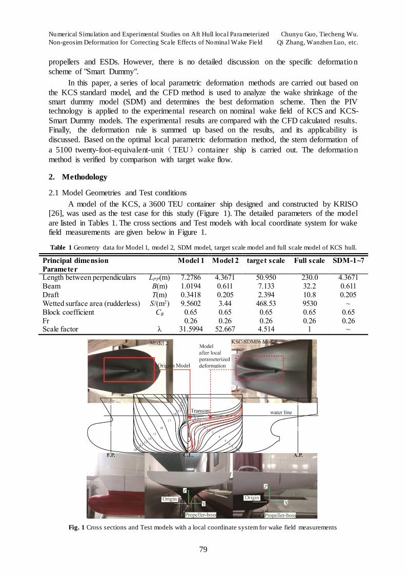
A model of the KCS, a 3600 TEU container ship designed and constructed by KRISO [26], was used as the test case for this study (Figure 1). The detailed parameters of the model
are listed in Tables 1. The cross sections and Test models with local coordinate system for wake field measurements are given below in Figure 1.
Table 1 Geometry data for Model 1, model 2, SDM model, target scale model and full scale model of KCS hull.
Principal dimension Parameter
Model 1 Model 2 target scale Full scale SDM-1~7
Length between perpendiculars LPP(m) 7.2786 4.3671 50.950 230.0 4.3671 Beam B(m) 1.0194 0.611 7.133 32.2 0.611 Draft T(m) 0.3418 0.205 2.394 10.8 0.205 Wetted surface area (rudderless) S/(m2) 9.5602 3.44 468.53 9530 ~ Block coefficient CB 0.65 0.65 0.65 0.65 0.65 Fr 0.26 0.26 0.26 0.26 0.26 Scale factor λ 31.5994 52.667 4.514 1 ~
Fig. 1 Cross sections and Test models with a local coordinate system for wake field measurements
Chunyu Guo, Tiecheng Wu. Numerical Simulation and Experimental Studies on Aft Hull local Parameterized
Qi Zhang, Wanzhen Luo, etc. Non-geosim Deformation for Correcting Scale Effects of Nominal Wake Field
80
2.2 Numerical Model and Mesh Partitioning
2.2.1 Governing Equations
The motion-compliant continuity and momentum conservation equations for
incompressible Newtonian fluid motion [27] are as follows:
0
i
i
u
t x
(1)
i i
i j i j jj j j j
u upu u u u S
t x x x x
(2)
where ui and uj are the time-averaged values (i, j = 1, 2, 3) of the velocity component; p
is the time-averaged value of the pressure; ρ is the fluid density; μ is the dynamic viscosity
coefficient; i ju u is the Reynolds stress term; and Sj is the source term, in this paper, a
numerical wave beach is a wave damping source term (See section 2.2.3).
2.2.2 Turbulence Model and Treatment of Free Surface
In the analysis, a computational finite volume method is used to analyze the cases of KCS
hull, SDM-KCS and 5100 TEU hull in this paper by using a segregated flow solver. The formulation is fully coupled and based on pressure, with second-order upwind spatial discretization being used for the convective flux terms and second-order central discretiza t ion
being used for the diffusion terms. An implicit pseudo time-marching scheme is used to determine a steady-state solution. Preconditioning is used to make this approach suitable for low-speed, isothermal flows [28] (Weiss, 1995). A point-implicit (Gauss-Seidel) linear system
solver is used with algebraic multigrid acceleration to solve the resulting discrete linear system at each iteration. The shear stress transport k model [29] (Menter, 1994) is used in this
study to simulate the strong adverse pressure gradient flow field with considering the impact of
the shear force exerted by the wall of the model. The free surface is modeled using the two-phase volume of fluid (VOF) technique [30] (Hirt, 1981).
2.2.3 Wave Damping
A numerical wave beach was established at the inlet, outlet, and side boundaries of the tank to avoid reflection. Waves can be damped by introducing resistance to vertical motion.
The method devised by Choi and Yoon [31] adds a resistance term to the equation for w -
velocity:
1 2 1
1
1
dz
eS f f w w
e
(3)
with
dn
sd
ed sd
x x
x x
(4)
where sdx is the starting point for wave damping (propagation in the x-direction); edx is the
end point for wave damping (boundary); 1f , 2f , and dn are the parameters of the damping model;
and w is the vertical velocity component.

Numerical Simulation and Experimental Studies on Aft Hull local Parameterized Chunyu Guo, Tiecheng Wu.
Non-geosim Deformation for Correcting Scale Effects of Nominal Wake Field Qi Zhang, Wanzhen Luo, etc.
81
2.2.4 CFD Mesh
All trimmed meshes were generated using STAR-CCM+: five meshes of varying resolutions for the model 1 case and grid-independent validation, and two single “medium”
density meshes for the model 2 and target scale conditions, another two single “medium” density meshs for the model 5100 TEU and its target scale model. A summary of the key mesh parameters is presented in Table 4.
Through the use of arbitrarily shaped volumetric control regions, the volume mesh was refined in different ways, as illustrated in Figure 2, which shows different cross-sectional views.
The first is the overall mesh for the KCS. A Kelvin mesh refinement was defined in the region of the Kelvin wave system to capture the wave pattern and better resolve the water/air layer interaction. A robust automated prism layer meshing algorithm was used to capture the
boundary layer, with a two-layer all y+ wall treatment. The y+ values were kept in the 30–300 range [1] [32].
The computational domain (Figure 3) was -1.0 LPP ≦ x ≦ 4.0 LPP, 0.0 LPP ≦ y ≦ 1.5
LPP, and -1.0 LPP ≦ z ≦ 2.0 LPP. The coordinate system for comparison was fixed to x = 0.0
(FP) on the undisturbed water plane. The boundary conditions are listed in Table 2.
Fig. 2 Details of the CFD mesh used in this study. (a) Overall mesh. (b) Mesh area of the Kelvin wave
system. (c) Prismatic boundary layer mesh of the bow. (d) Prismatic boundary layer mesh of the stern.
Fig. 3 Computational domain used to determine the boundary conditions for the test case in this study.
Table 2 Boundary parameters.
Boundary Boundary Parameter
Inlet Inlet with a flat VOF-wave defined volume fraction. Flow speed is 1.701, 2.196,
5.810 m/s for KCS and SDM hull, 1.251, 4.277 m/s for 5100 TEU hull. Turbulence intensity 0.01
Outlet Outlet with hydrostatic pressure of flat vof wave Bottom/side/top Same as inlet
Ship Wall with no slip condition Symmetry plane Along centerline of hull
2.3 Local parameterized deformation
The deformation method for modifying the aft-hull of the KCS ship model with LPP =
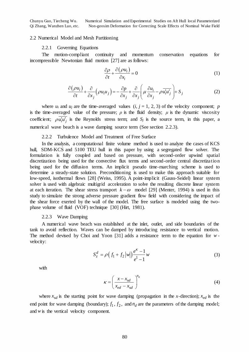
4.367 m is based on the localized method of parametric deformation. A B-spline surface was built on the central vertical section of the stern, and 5*5 control points (CPs) (5 CPs in U-
direction, 5 CPs in V-direction) were set to manage the changes in this surface. By moving one or more control points, the shape of the B-spline surface can be changed, and the shape of the aft hull can thereby be modified. The hull is divided into 20 frames along the length direction.
The sections of deformation are identified using their frame numbers. Setting the center of the propeller plan as a starting point in the height direction, two rows of control points are arranged
Chunyu Guo, Tiecheng Wu. Numerical Simulation and Experimental Studies on Aft Hull local Parameterized
Qi Zhang, Wanzhen Luo, etc. Non-geosim Deformation for Correcting Scale Effects of Nominal Wake Field
82
at the upper 23% T and lower 9.5% T (where T represents the designed draught). A schematic
of the deformation control is shown in Figure 4.
Fig. 4 Schematic of the deformation control surface configured from frame 1.5 to the exit of the stern shaft
2.3.1 Basis functions of B-spline
B-spline basis functions are defined recursively starting with piecewise constants (p = 0)
1,0
1 ,
0 otherwise.
i ii
ifN
(5)
For p = 1, 2, 3…, they are defined by
1, , 1 1, 1
1 1
.i i Pi p i p i p
i p i i p i
N N N
(6)
Derivatives with respect to spatial coordinates may be computed by way of standard
techniques described in Hughes [32, Chapter 3][33].
2.3.2 B-spline curves
B-spline curves in d are constructed by taking a linear combination of B-spline basis
functions. The coefficients of the basis functions are referred to as control points. These are somewhat analogous to nodal coordinates in finite element analysis. Piecewise linear
interpolation of the control points gives the so-called control polygon. In general, control points are not interpolated by B-spline curves. Given n basis functions, Ni,p, i = 1,2,. . . ,n, and
corresponding control points Bi ∈ d , i =1, 2, …, n, a piecewise-polynomial B-spline curve
[32, Chapter 3] [33]is given by
,
1
.n
i p i
i
C N B
(7)
2.3.3 B-spline surface
Given a control net {Bi,j}, i = 1,2,…,n, j = 1,2,…,m, and knot vectors
1 2 1= , , . . . , n p , and 1 2 1= , , . . . , n p , a tensor product B-spline surface is
defined by
, , ,
1 1
, ( ) ,n m
i p j q i j
i j
S N M B
(8)

Numerical Simulation and Experimental Studies on Aft Hull local Parameterized Chunyu Guo, Tiecheng Wu.
Non-geosim Deformation for Correcting Scale Effects of Nominal Wake Field Qi Zhang, Wanzhen Luo, etc.
83
where Ni,p and Mj,q are basis functions of B-spline curves, i is the i th it knot, i is the
knot index, i = 1,2,…, n+p+1, p is the polynomial order, and n is the number of basis functions
which comprise the B-spline[32, Chapter 3][33].
2.4 Test Equipment and Measurement Methods
2.4.1 Towing tank
PIV measurements of the wake fields of the model 2 and KCS-SDM06 were performed in the towing-tank laboratory for ship models at Harbin Engineering University. The
specifications of the laboratory equipment are as follows:
Towing tank: 108 m (length) × 7 m (width) × 3.5 m (depth);
Trailer: steady speed range of 0.1–6.5 m/s and accuracy of 0.1%;
Motion recorder with four degrees of freedom (DOF) (Japan): model = GEL-421-1; measurement range = F ≤ 100 N; measurable heave = ±200 mm; surging = ±400 mm; roll angle
= ±50°; pitch angle = ±50°; accuracy = 0.1%.
2.4.2 DANTEC vehicle- loaded underwater PIV measurement system
The DANTEC vehicle- loaded PIV measurement system was used to measure the wake fields of the model 2 and KCS-SDM06. The schematic diagram of the measurement system is shown in Figure 5. PIV test conditions are listed in Tables 3. The section of the ship’s wake
field being measured is the propeller plan (x/ LPP = 0.0175, where x/ LPP = 0 is the stern). The local coordinate system of the wake field region is shown in Figure 1. The specifications of this
system are as follows:
CCD resolution: 2048 × 2048 pixels; Maximum pulse energy of laser: 200 mJ;
Duration of laser beam: 4 ns; Wavelength of laser: 532–1064 nm;
Thickness of light sheet: 0.6 mm; The largest size of the measurement area: 400 × 400 mm; PIV tracer particles: polyamide tracer particles (PSP-50μm).
Table 3 PIV test conditions
Parameter KCS Mode 2 KCS-SDM06 Model Testing cross section Propeller plan Propeller plan Designed draught/m 0.205 0.205
Liquid medium Water Water Speed Vm / (m/s) 1.701 1.701
Wave Flat water surface Flat water surface
Fig. 5 PIV system and schematic diagram of the measurement system for a ship model’s wake field

Chunyu Guo, Tiecheng Wu. Numerical Simulation and Experimental Studies on Aft Hull local Parameterized
Qi Zhang, Wanzhen Luo, etc. Non-geosim Deformation for Correcting Scale Effects of Nominal Wake Field
84
3. Mesh Sensitivity Study
The level of the mesh density was changed by adjusting the base size of the grids, while keeping the other settings unchanged. As shown above, the meshes generated for the KCS ship
model with LPP = 7.2786 m using a base size of 0.075 (100% base size) for a routine model gave relatively satisfying results. The base size of the grids was then changed to 0.17 (226%), 0.14 (187%), 0.095 (127%), and 0.05 (67%) to generate 0.47, 0.66, 1.37, and 5.40 million grids,
respectively. These meshes are either coarser or denser than that obtained using the normal number of grids (usually 2 to 4 million) for a regular model scale (half ship). To carry out the
grid Sensitivity study, the grid refinement ratio, Gr , should be determined. In general, the
definition of Gr is the ratio of coarse to fine cell sizes, indicating that the refinement factor is
simple to compute for structured grid. However, in the present study, Cartesian cut-cell method was used to generate the computational mesh, the refinement ratio
Gr was considered as follows
[34]: 1/d
fine
G
coarse
Nr
N
(9)
where the total number of grids is noted as N, d is the dimensionality of the computing
problem and its value in the present study is 3. Roy et al. [34] presented methods for assessing the uniformity of the grid refinement with Cartesian grid. As a result, five grid systems considered in the present study was constructed based on method of Roy et al. [34] to uniformly
refine the grid over the entire domain in all three coordinate directions. The grid refinement factor for the fine/medium-1 (medium-1/medium-2, medium-2/coarse, coarse/very coarse)
grids is 1.32, 1.18, 1.27 and 1.12, respectively. The grid refinement ratio of fine to medium (medium to coarse) grids is approximately 1.2, which is consistent with Roy et al. [34].A comparison of the differences among the five mesh scenarios can be obtained from the
perspectives of the resistance coefficient and wake field distribution.
The numerical prediction results obtained from the meshes were compared with the
experimental data. Figure 6 shows that the resulting predicted values are in good agreement with the experimentally measured values [35], which indicates the reliability of the predicted numerical results.
Fig. 6 Nominal wake distribution (1-w) at propeller plan of Model 1(KCS), where the left part shows the
calculated values and the right part shows the measured values
Numerical Simulation and Experimental Studies on Aft Hull local Parameterized Chunyu Guo, Tiecheng Wu.
Non-geosim Deformation for Correcting Scale Effects of Nominal Wake Field Qi Zhang, Wanzhen Luo, etc.
85
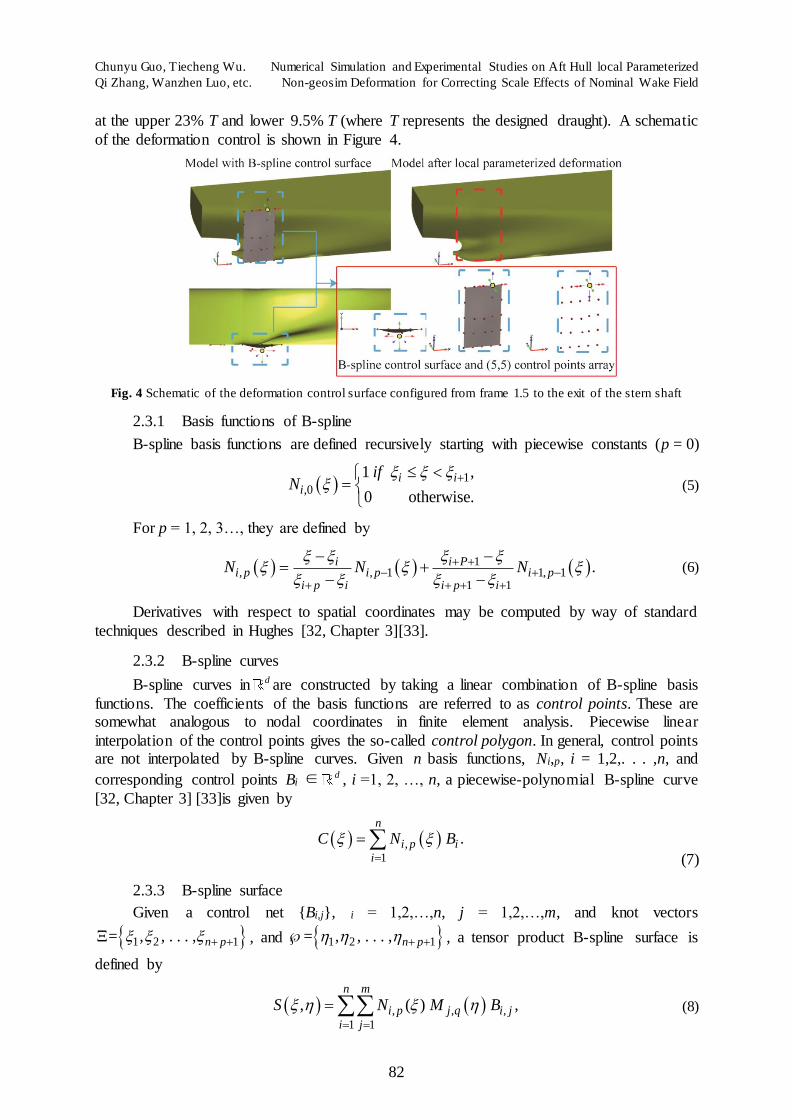
Table 4 Comparison of resistance coefficients under different numbers of grids
Mesh number Residual Resistance coefficient
(10-3)
Friction Resistance coefficient
(10-3)
Total Resistance coefficient
(10-3)
Error(%)
EFD data -- -- 3.550 -- 0.47 million 0.709 2.868 3.577 0.761 0.66 million 0.680 2.889 3.569 0.535 1.37 million 0.646 2.915 3.561 0.309 2.30 million 0.634 2.915 3.549 -0.028 5.41 million 0.628 2.920 3.548 -0.056
Table 4 lists the comparisons between the calculation results with different levels of mesh
density and experimental data. The table indicates that although the five mesh scenarios are under different levels of density, the calculated resistance results for all meshes were fairly accurate, with an error of less than 1% compared to the measured value. When making
comparisons after dividing the total resistance coefficient into the residual resistance and friction resistance coefficients, it can be observed from the above table that the mesh density
has a minor impact on the friction resistance coefficient, whereas the residual resistance coefficient presents a certain level of fluctuation along with changes in the mesh density. In particular, the mesh scenarios with 0.47 and 0.66 million grids show more apparent fluctuat ions
in the residual resistance coefficient, which suggests that the residual resistance is more sensitive to the changes in mesh density.
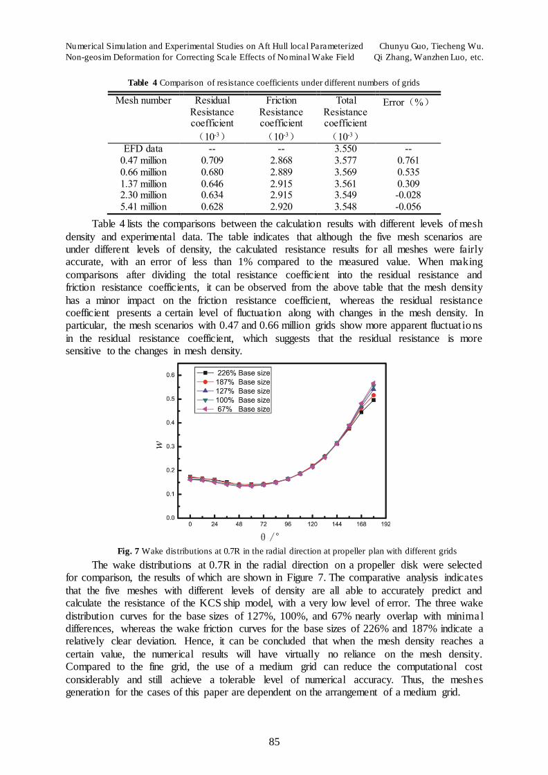
Fig. 7 Wake distributions at 0.7R in the radial direction at propeller plan with different grids
The wake distributions at 0.7R in the radial direction on a propeller disk were selected for comparison, the results of which are shown in Figure 7. The comparative analysis indicates
that the five meshes with different levels of density are all able to accurately predict and calculate the resistance of the KCS ship model, with a very low level of error. The three wake
distribution curves for the base sizes of 127%, 100%, and 67% nearly overlap with minimal differences, whereas the wake friction curves for the base sizes of 226% and 187% indicate a relatively clear deviation. Hence, it can be concluded that when the mesh density reaches a
certain value, the numerical results will have virtually no reliance on the mesh density. Compared to the fine grid, the use of a medium grid can reduce the computational cost
considerably and still achieve a tolerable level of numerical accuracy. Thus, the meshes generation for the cases of this paper are dependent on the arrangement of a medium grid.

Chunyu Guo, Tiecheng Wu. Numerical Simulation and Experimental Studies on Aft Hull local Parameterized
Qi Zhang, Wanzhen Luo, etc. Non-geosim Deformation for Correcting Scale Effects of Nominal Wake Field
86
4. Numerical Simulations with Models of Different Scales
Given that the number of grids for a full scale ship (LPP = 230m) imposes high demands on the computational performance, in this section, the wake fields of the two models are
calculate using different scale models, i.e., using different lengths between perpendiculars LPP = 4.3671 and 50.95 m, the latter of which is treated as a target-scale model for this research. The detailed parameters of the models are listed in Table 5.
Table 5. Major parameters of the numerical models
KCS LPP / m Bwl / m T / m Cb V/ (m·s-1) Wet area/ m2 Re*10-6
Model 2 4.367 0.611 0.205 0.651 1.701 3.44 7.4 Target scale 50.950 7.133 2.394 0.651 5.810 468.53 294.9
The grid was created with reference to the above-mentioned grid methods for a KCS
model. Owing to the difference in ship model scales, there are certain differences in the number of grids, as well as the thickness and numbers of boundary layers between the two models.
Specific values of the thickness of the first-layer boundary, y+, and the total number of grids for the two models are listed in Table 6. The resistance data obtained from the results of the numerical calculations are listed in Table 7.
Table 6 Number of grids and boundary layer setting for each model
Model 2 Target scale
First-layer boundary layer /mm 1.31 0.62 Number of layers for boundary layer 7 15 y plus(max) 80 150
Total number of grids(in millions) 198 472
Table 7 Comparison of the calculations of convergence and resistance for each model
Model 2 Target scale
Time in convergence/s 70 300 Total resistance coefficient CT/10-3 4.08 2.61 Converted to full-scale CT
, /10-3 2.54 2.43 CT error(exact value 2.334[19]) +8.80% +4.11%
The resistance coefficient conversion is implemented using the two-dimensiona l
conversion method, where the roughness allowance coefficient, FC , is calculated based on
the equation recommended by ITTC, as shown in Eq. (9). The exact value of the total resistance
coefficient for a full scale ship (LPP = 230 m) was adopted from the CFD calculation results of a previous study [19].
1/3 3[105( / ) 0.64] 10F sC k L (10)
where ks represents the apparent height of the roughness, which can be set as ks = 150×10-
6 m, and L represents the ship length.
In order to make a Verification and Validation of the PIV test data of this paper. Figure 8
illustrated the comparison of mean axial velocity at the propeller plane between current result (PIV) and the result of Kim's pitot-tube experiment [35]. Good agreement is achieved.

Numerical Simulation and Experimental Studies on Aft Hull local Parameterized Chunyu Guo, Tiecheng Wu.
Non-geosim Deformation for Correcting Scale Effects of Nominal Wake Field Qi Zhang, Wanzhen Luo, etc.
87
Fig. 8 Wake on plane of propeller disc at design condition (Left: Kim et al [35].; right: this paper)
To compare the state of agreement between flow-field CFD calculations and the
experimental data, the nominal wake field distributions of the models were compared. As shown in Figure 9, the measured and calculated wake fields on the propeller plan for the KCS
ship model under the designed speed are in good agreement. Moreover, the measured and calculated circumferential distributions of the model’s axial wake at 0.7R also essentia lly overlap.
Fig. 9 Comparisons of Wake distribution and circumferential wake distributions (0.7R) between CFD results and
PIV data (right) for the KCS ship model (Vm = 1.701 m/s)
Model 2 Lpp=4.367m Target scale Lpp=50.950m
Fig. 10 Axial nominal wake distributions for models of different scales

Chunyu Guo, Tiecheng Wu. Numerical Simulation and Experimental Studies on Aft Hull local Parameterized
Qi Zhang, Wanzhen Luo, etc. Non-geosim Deformation for Correcting Scale Effects of Nominal Wake Field
88
Figure 10 shows the wake field distributions for the two models with scales of LPP = 4.367
and 50.950 m. The figure shows that the target-scale model exhibits a significant contraction of the wake field compared to the other model. In addition, given the lack of experimental data for
the wake field of the target-scale model (LPP = 50.95 m), the reliability of the flow-fie ld calculations can be validated with the help of the resistance data results. The error is less than 5% (table 7) when converting the resistance value of the target-scale model to a full-scale KCS
ship [19], meeting the accuracy requirement of the resistance calculation.
5. Aft Hull Deformation Schemes
5.1 Deformation Schemes with Different Frame Section Spaces
To investigate the effects of contractual deformation at different aft sections on the wake field, the deformation schemes set from frames 1, 1.5, and 2.5 to the stern shaft are
demonstrated. The deformed models are named SDM01, SDM02, and SDM03, respectively. The aim of this study is to explore the best position of deformation, and to do the basic research
for the next study of deformation schemes different degrees of contraction. The change of molded lines and wake distribution between the SDM model and the original model are shown in Figure 11-13.
Fig. 11 Comparisons of molded lines and Wake distribution between the SDM01 and the original model
Fig. 12 Comparisons of molded lines and Wake distribution between the SDM02 and the original model
Numerical Simulation and Experimental Studies on Aft Hull local Parameterized Chunyu Guo, Tiecheng Wu.
Non-geosim Deformation for Correcting Scale Effects of Nominal Wake Field Qi Zhang, Wanzhen Luo, etc.
89
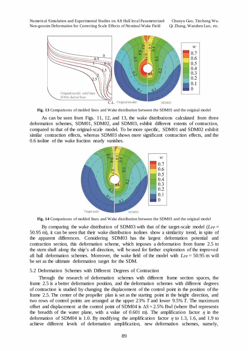
Fig. 13 Comparisons of molded lines and Wake distribution between the SDM03 and the original model
As can be seen from Figs. 11, 12, and 13, the wake distributions calculated from three deformation schemes, SDM01, SDM02, and SDM03, exhibit different extents of contraction,
compared to that of the original-scale model. To be more specific, SDM01 and SDM02 exhibit similar contraction effects, whereas SDM03 shows more significant contraction effects, and the 0.6 isoline of the wake fraction nearly vanishes.
Fig. 14 Comparisons of molded lines and Wake distribution between the SDM03 and the original model
By comparing the wake distribution of SDM03 with that of the target-scale model (LPP = 50.95 m), it can be seen that their wake distribution isolines show a similarity trend, in spite of the apparent differences. Considering SDM03 has the largest deformation potential and
contraction section, this deformation scheme, which imposes a deformation from frame 2.5 to the stern shaft along the ship’s aft direction, will be used for further exploration of the improved
aft hull deformation schemes. Moreover, the wake field of the model with LPP = 50.95 m will be set as the ultimate deformation target for the SDM.
5.2 Deformation Schemes with Different Degrees of Contraction
Through the research of deformation schemes with different frame section spaces, the frame 2.5 is a better deformation position, and the deformation schemes with different degrees
of contraction is studied by changing the displacement of the control point in the position of the frame 2.5. The center of the propeller plan is set as the starting point in the height direction, and two rows of control points are arranged at the upper 23% T and lower 9.5% T. The maximum
offset and displacement at the control point of SDM04 is ∆S = 2.5% Bwl (where Bwl represents the breadth of the water plane, with a value of 0.601 m). The amplification factor η in the
deformation of SDM04 is 1.0. By modifying the amplification factor η to 1.3, 1.6, and 1.9 to achieve different levels of deformation amplification, new deformation schemes, namely,

Chunyu Guo, Tiecheng Wu. Numerical Simulation and Experimental Studies on Aft Hull local Parameterized
Qi Zhang, Wanzhen Luo, etc. Non-geosim Deformation for Correcting Scale Effects of Nominal Wake Field
90
SDM05, SDM06, and SDM07. The change of molded lines and wake distribution between the
SDM model and the target model are shown in Figure 15-18.
Fig. 15 Comparisons of molded lines and Wake distribution between the SDM03 and the original model
Fig. 16 Comparisons of molded lines and Wake distribution between the SDM03 and the original model
Fig. 17 Comparisons of molded lines and Wake distribution between the SDM03 and the original model

Numerical Simulation and Experimental Studies on Aft Hull local Parameterized Chunyu Guo, Tiecheng Wu.
Non-geosim Deformation for Correcting Scale Effects of Nominal Wake Field Qi Zhang, Wanzhen Luo, etc.
91
Fig. 18 Comparisons of molded lines and Wake distribution between the SDM03 and the original model
Figure 15-18 show four schematics of wake isoline changes matching the four deformation
schemes with various degrees of contraction, which are obtained from a large number of numerical calculations. As demonstrated in Figure 15, the wake field of SDM04 apparently has a higher degree of contraction than that of SDM03 (particularly in the upper part of the disk).
However, it still differs somewhat from the wake field of the full-scale model. SDM05 and SDM06, which have deformation control factors within the range of 1.3-1.6, show a fairly
satisfactory contraction effect, especially in the upper part of the disk above its center. SDM07 continues to contract. When the deformation control factor reaches 1.9, as shown in Figure 18, the 0.5 isoline has already discontinued. This deformation scheme is undesirable because the
degree of contraction exceeds the requirement of the target wake field. Therefore, among these four typical deformation schemes, it is clear that SDM05 and SDM06 are in better agreement
with the target wake field.
Through the modifications of speed increase [10] of SDM05 and SDM06, their wake fields may become even closer to that of the full-scale model. Now, by manually increasing the
wake velocity on the propeller disk by 5%, we can modify the circumferential distributions of an axial wake at 0.7R for SDM05 and SDM06, as shown in Figure 20. The modified wake
distributions and other numerical values for both the deformation schemes are extremely close to the targets, except for values under 24°.
Fig. 19 Modified circumferential distribution of the axial wake at 0.7R for SDM05 (left) and SDM06 (right)
To compare the state of agreement between flow-field CFD calculations and the
experimental data, the nominal wake field distributions of the SDM-model were compared. As shown in Figure 20, for the aft-shape modified KCS-SDM06 ship model, the measured and calculated wake distributions on the propeller disk under the designed speed are generally the
Chunyu Guo, Tiecheng Wu. Numerical Simulation and Experimental Studies on Aft Hull local Parameterized
Qi Zhang, Wanzhen Luo, etc. Non-geosim Deformation for Correcting Scale Effects of Nominal Wake Field
92
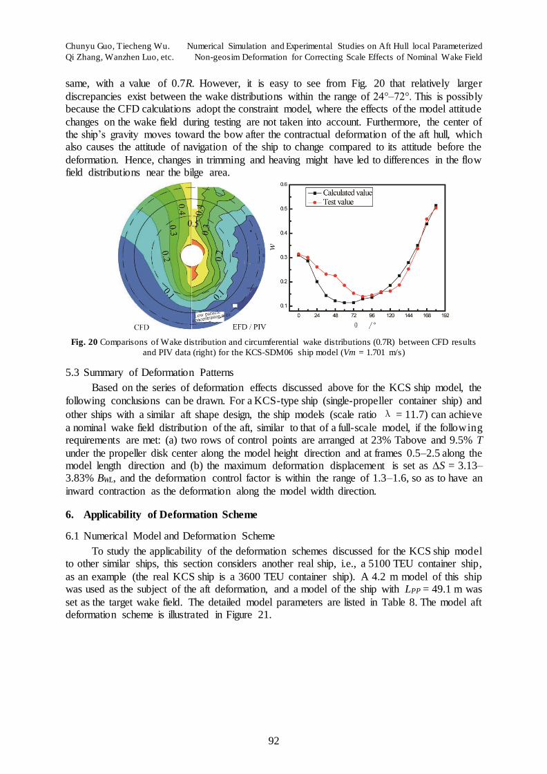
same, with a value of 0.7R. However, it is easy to see from Fig. 20 that relatively larger
discrepancies exist between the wake distributions within the range of 24°–72°. This is possibly because the CFD calculations adopt the constraint model, where the effects of the model attitude
changes on the wake field during testing are not taken into account. Furthermore, the center of the ship’s gravity moves toward the bow after the contractual deformation of the aft hull, which also causes the attitude of navigation of the ship to change compared to its attitude before the
deformation. Hence, changes in trimming and heaving might have led to differences in the flow field distributions near the bilge area.
Fig. 20 Comparisons of Wake distribution and circumferential wake distributions (0.7R) between CFD results
and PIV data (right) for the KCS-SDM06 ship model (Vm = 1.701 m/s)
5.3 Summary of Deformation Patterns
Based on the series of deformation effects discussed above for the KCS ship model, the
following conclusions can be drawn. For a KCS-type ship (single-propeller container ship) and
other ships with a similar aft shape design, the ship models (scale ratio λ = 11.7) can achieve
a nominal wake field distribution of the aft, similar to that of a full-scale model, if the following requirements are met: (a) two rows of control points are arranged at 23% Tabove and 9.5% T
under the propeller disk center along the model height direction and at frames 0.5–2.5 along the model length direction and (b) the maximum deformation displacement is set as ∆S = 3.13–3.83% BWL, and the deformation control factor is within the range of 1.3–1.6, so as to have an
inward contraction as the deformation along the model width direction.
6. Applicability of Deformation Scheme
6.1 Numerical Model and Deformation Scheme
To study the applicability of the deformation schemes discussed for the KCS ship model to other similar ships, this section considers another real ship, i.e., a 5100 TEU container ship,
as an example (the real KCS ship is a 3600 TEU container ship). A 4.2 m model of this ship was used as the subject of the aft deformation, and a model of the ship with LPP = 49.1 m was
set as the target wake field. The detailed model parameters are listed in Table 8. The model aft deformation scheme is illustrated in Figure 21.

Numerical Simulation and Experimental Studies on Aft Hull local Parameterized Chunyu Guo, Tiecheng Wu.
Non-geosim Deformation for Correcting Scale Effects of Nominal Wake Field Qi Zhang, Wanzhen Luo, etc.
93
Table 8 Major parameters of the 5100 TEU ship model
Parameter Full scale Target scale Model scale SDM-5100
TEU Scale ratio λ 1.00 5.79 67.66 67.66
LPP / m 284.16 49.1 4.2 4.2 BW L / m 32.2 5.561 0.475 0.475
T / m 12.0 2.07 0.177 0.177 V/ (m·s-1) 10.29 4.277 1.251 1.251
CB 0.63 0.63 0.63 ~ Re 2.913*109 2.092*108 5.234*106 5.234*106 Fr 0.194 0.194 0.194 0.194
Fig. 21 5100 TEU container ship model and stern lines with SDM08 and the original model (∆S = 3.47% BW L)
6.2 Analysis of wake field calculations
λ=67.66 LPP =4.2m λ=5.79 LPP =49.1m
Fig. 22 Distributions of the axial nominal wake field of model scale and target scale of 5100 TEU container ship
Chunyu Guo, Tiecheng Wu. Numerical Simulation and Experimental Studies on Aft Hull local Parameterized
Qi Zhang, Wanzhen Luo, etc. Non-geosim Deformation for Correcting Scale Effects of Nominal Wake Field
94
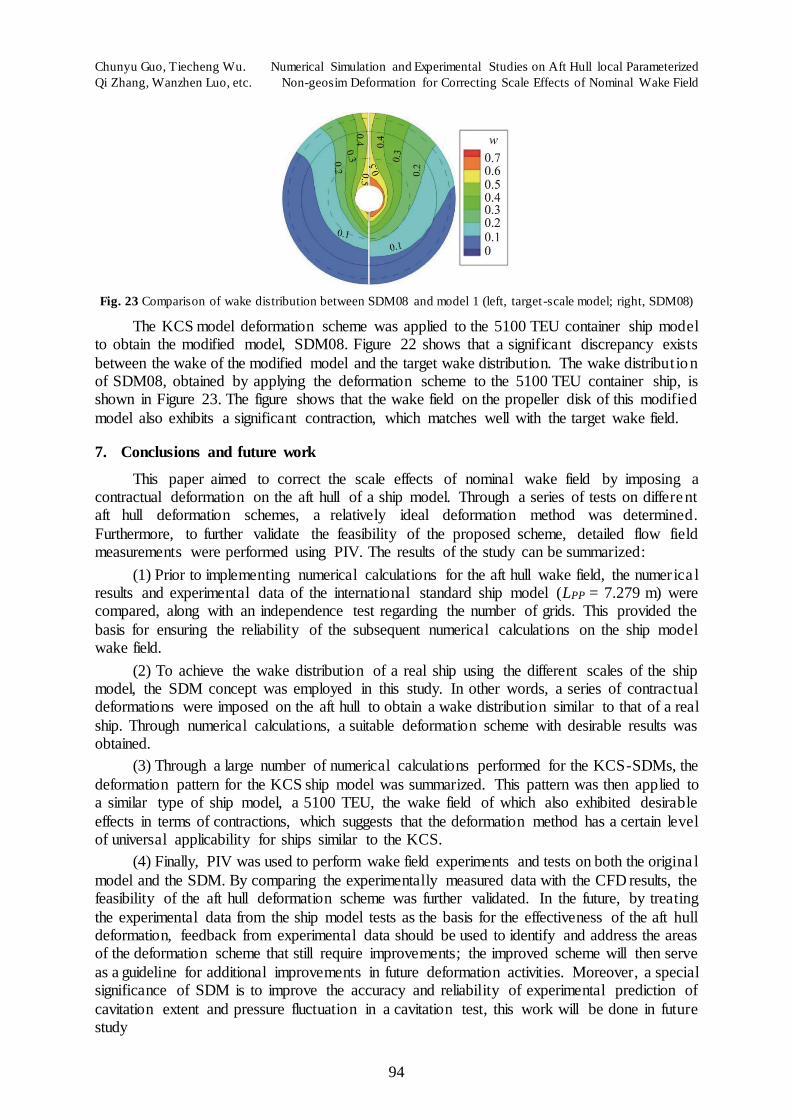
Fig. 23 Comparison of wake distribution between SDM08 and model 1 (left, target -scale model; right, SDM08)
The KCS model deformation scheme was applied to the 5100 TEU container ship model to obtain the modified model, SDM08. Figure 22 shows that a significant discrepancy exists
between the wake of the modified model and the target wake distribution. The wake distribution of SDM08, obtained by applying the deformation scheme to the 5100 TEU container ship, is shown in Figure 23. The figure shows that the wake field on the propeller disk of this modified
model also exhibits a significant contraction, which matches well with the target wake field.
7. Conclusions and future work
This paper aimed to correct the scale effects of nominal wake field by imposing a contractual deformation on the aft hull of a ship model. Through a series of tests on different aft hull deformation schemes, a relatively ideal deformation method was determined.
Furthermore, to further validate the feasibility of the proposed scheme, detailed flow field measurements were performed using PIV. The results of the study can be summarized:
(1) Prior to implementing numerical calculations for the aft hull wake field, the numerica l results and experimental data of the international standard ship model (LPP = 7.279 m) were compared, along with an independence test regarding the number of grids. This provided the
basis for ensuring the reliability of the subsequent numerical calculations on the ship model wake field.
(2) To achieve the wake distribution of a real ship using the different scales of the ship model, the SDM concept was employed in this study. In other words, a series of contractual deformations were imposed on the aft hull to obtain a wake distribution similar to that of a real
ship. Through numerical calculations, a suitable deformation scheme with desirable results was obtained.
(3) Through a large number of numerical calculations performed for the KCS-SDMs, the
deformation pattern for the KCS ship model was summarized. This pattern was then applied to a similar type of ship model, a 5100 TEU, the wake field of which also exhibited desirable
effects in terms of contractions, which suggests that the deformation method has a certain level of universal applicability for ships similar to the KCS.
(4) Finally, PIV was used to perform wake field experiments and tests on both the origina l
model and the SDM. By comparing the experimentally measured data with the CFD results, the feasibility of the aft hull deformation scheme was further validated. In the future, by treating
the experimental data from the ship model tests as the basis for the effectiveness of the aft hull deformation, feedback from experimental data should be used to identify and address the areas of the deformation scheme that still require improvements; the improved scheme will then serve
as a guideline for additional improvements in future deformation activities. Moreover, a special significance of SDM is to improve the accuracy and reliability of experimental prediction of
cavitation extent and pressure fluctuation in a cavitation test, this work will be done in future study

Numerical Simulation and Experimental Studies on Aft Hull local Parameterized Chunyu Guo, Tiecheng Wu.
Non-geosim Deformation for Correcting Scale Effects of Nominal Wake Field Qi Zhang, Wanzhen Luo, etc.
95
8. Acknowledgments
This project was supported by the National Natural Science Foundation of China (Grant Nos. 41176074, 51209048, 51379043 and 51409063), the Fundamental Research Funds for the
Central Universities (Grant No. P013513013), and the Specialized Research Fund for the Doctoral Program of Higher Education (Grant No. 20102304120026).
REFERENCES
[1] Wang. Z. Z., Xiong. Y., Wang. R., Shen. X. R., Zhong. C. H, “Numerical Study on Scale Effect of
Nominal Wake of Single Screw Ship”, Ocean Engineering, 2015.104, 437-451.
[2] Schneekluth H., “Wake Equalization Duct”, the Naval Architect, 1986.
[3] Stierman E. J., “The Design of an Energy Saving, Wake Adapted Duct”, Proceedings of International
Symposium on Practical Design of Ships and other Floating Structures PRADS, 1987. Trondheim,
Norway.
[4] Hansen H. R., Dinham-Peren T. & Nojiri T. “Model and Full Scale Evaluation of a ‘Propeller Boss
Cap Fins’ Device Fitted to an Aframax Tanker”, Proceedings of 2nd International Symposium on Marine
Propulsors, SMP’11. 2011, Hamburg, Germany.
[5] Lee, J. T., Kim, M. C., Suh, J. C., Kim, S. H. & Choi, J. K., “Development of a Preswirl Stator-Propeller
System for Improvement of Propulsion Efficiency: a Symmetric Stator Propulsion System”, Transaction
of SNAK, No. 29(4), 1992, Busan, Korea.
[6] Mewis F. & Guiard Th., “Mewis Duct® - New Developments, Solutions and Conclusions”, Proceedings
of 2nd International Symposium on Marine Propulsors, SMP’11. 2011, Hamburg, Germany.
[7] Dang J., Chen H., Dong G., van der Ploeg A., Hallmann R. and Mauro F., “An Exploratory Study on the
Working Principles of Energy Saving Devices (ESDs)”, Proceedings of International Symposium on
Green Ship Technology, Greenship’2011, Wuxi, China. (available on www.marin.nl)
[8] Dang J., Dong G., chen H., “AN EXPLORATORY STUDY ON THE WORKING PRINCIPLES OF
ENERGY SAVING DEVICES (ESDS) – PIV, CFD INVESTIGATIONS AND ESD DESIGN
GUIDELINES” , Proceedings of the 31st International Conference on Ocean, Offshore and Arctic
Engineering OMAE2012 July 01-06, 2012, Rio de Janeiro, Brazil.
[9] Zhao. Q. X., Guo. C. Y. & Zhao. D. G.., “Study on self-propulsion experiment of ship model with
energy-saving devices based on numerical simulation methods ”, Ships and Offshore Structures, 2015,
10:6, 669-677. https://doi.org/10.1080/17445302.2014.945765.
[10] Schuiling, B., Lafeber, F. H., Ploeg, A. V. D., & Wijngaarden, E. V., “The Influence of the Wake Scale
Effect on the Prediction of Hull Pressures due to Cavitating Propellers ”, Proceedings of 2nd International
Symposium on Marine Propulsors, SMP’11. 2011, Hamburg, Germany.
[11] Mehlhorn, T., “Verfahren zur Berücksichtigung des Maßstabseffekts auf den Nachstrom Internationales
Schiffstechnisches Symposium”, Rostock, Nov. 1983
[12] Hoekstra H., “Prediction of Full Scale Wake Characteristics Based on Model Wake Survey”,
International Shipbuilding Progress, Vol. 22, 1975.
[13] Sasajima, H. and Tanaka, I., “On the estimation of wakes of ships”, XI ITTC, 1966, Tokyo.
[14] Tanaka I., “Scale Effects on Wake Distribution and Viscous Pressure Resistance of Ships” , Journal of
Kansai SNAJ, n.146, 1979.
[15] García Gómez A., “Predicción y Análisis de la Configuracion de la Estela en Buques de una Hélice” PhD
Thesis, Universidad Politénica de Madrid, 1989.
[16] García Gómez A., “On the Form Factor Scale” Ocean Engineering January 2000, 25th International
Towing Tank Conference, The Specialist Committee on Powering Performance Prediction Report,
Fukuoka, 2008.
[17] The Specialist Committee on Scaling of Wake Field. Final report and recommendations to the 26rd ITTC
[C]// Proceedings of 26rd ITTC. Rio de Janriro, Brazil: ITTC, 2011:379-417.
[18] Tezdogan, T., Demirel, Y. K., Kellett, P., Khorasanchi, M., Incecik, A., & Turan, O., “Full-scale unsteady
RANS CFD simulations of ship behaviour and performance in head seas due to slow steaming”, Ocean
Engineering, Volume 97, 15 March 2015, Pages 186-206.
https://doi.org/10.1016/j.oceaneng.2015.01.011.

Chunyu Guo, Tiecheng Wu. Numerical Simulation and Experimental Studies on Aft Hull local Parameterized
Qi Zhang, Wanzhen Luo, etc. Non-geosim Deformation for Correcting Scale Effects of Nominal Wake Field
96
[19] Castro, A. M., Carrica, P. M., & Stern, F., “Full scale self-propulsion computations using discretized
propeller for the KRISO container ship KCS”, Computers & Fluids, Volume 51, Issue 1, 15 December
2011, Pages 35-47. https://doi.org/10.1016/j.compfluid.2011.07.005.
[20] Bhushan, S., Xing, T., Carrica, P., Stern, F., “Model- and Full-scale URANS Simulations of Athena
Resistance, Powering, Seakeeping, and 5415 Maneuvering”, Journal of Ship Research, 2009, Vol. 53, No.
4, pp. 179-198.
[21] Atsavapranee P., Engle A., Grant D J., et al. “Full-Scale Investigation of Viscous Roll Damping with
Particle Image Velocimetry”[C], 27th Symposium on Naval Hydrodynamics, Seoul, Korea. 2008.
[22] Verkuyl, J.B. and Raven H.C., “Joint EFFORT for Validation of Full-Scale Viscous-Flow
Predictions”[R], The Naval Architect. 2003.
[23] Perelman, O., Fournier P., Mace R., Deuff J.B., DALIDA., “Development and Validation of Tools for
Hydrodynamic Signatures Prediction”[R], ATMT. 2012.
[24] Johannsen, C., Wijngaarden, E., “Investigation of Hull Pressure Pulses, Making Use of Two Large Scale
Cavitation Test Facilities”[C], 8th International Symposium on Cavitation (CAV), Singapore, 2012, pp.
196-202. https://doi.org/10.3850/978-981-07-2826-7_196.
[25] Bosschers, J., van Wijngaarden, E., “Scale Effects on Hull Pressure Fluctuations due to Cavitating
Propellers”[C], 10th International Conference on Hydrodynamics, Petersburg, Russia, 2012,pp. 26-30.
[26] Kim, J., “RANS computations for KRISO container ship and VLCC tanker using the WAVIS code”,
Proceedings of CFD Workshop (Tokyo), 2005, pp. 598-603.
[27] David C. Wilcox., “Turbulence Modeling for CFD. DOW Industries”, Inc. La Canada, California, 1994,
15-19p.
[28] Weiss, J.M. and Smith W.A., “Preconditioning applied to variable and constant density flows ”, Aiaa
Journal, 1995, 33(11), 2050-2057. https://doi.org/10.2514/3.12946.
[29] Menter, F.R., “Two-equation eddy-viscosity turbulence models for engineering applications ”, Aiaa
Journal, 1994, 32(8), 1598-1605. https://doi.org/10.2514/3.12149.
[30] Hirt, C.W. and Nichols, B.D., “Volume of fluid /VOF/ method for the dynamics of free boundaries”,
Journal of Computational Physics, 1981, 39(81), 201-225. https://doi.org/10.1016/0021-9991(81)90145-
5.
[31] Choi, J. and Yoon, S.B., “Numerical simulations using momentum source wave-maker applied to RANS
equation model”, Coastal Engineering, 2009, 56(10), 1043-1060.
https://doi.org/10.1016/j.coastaleng.2009.06.009.
[32] Hughes, T. J. R., “The Finite Element Method: Linear Static and Dynamic Finite Element Analysis ”,
Dover Publications, Mineola, NY, 2000.
[33] Hughes, T. J. R., Cottrell, J. A., & Bazilevs, Y., Isogeometric analysis: CAD, finite elements, NURBS,
exact geometry and mesh refinement, Computer Methods in Applied Mechanics and Engineering,
Volume 194, Issues 39–41, 1 October 2005, Pages 4135-4195. https://doi.org/10.1016/j.cma.2004.10.008.
[34] Roy CJ, Heintzelman C, Roberts SJ. Estimation of Numerical Error for 3D Inviscid Flows on Cartesian
Grids. 45th AIAA Aerosp Sci Meet Exhib Aerosp Sci Meet. 2007; (January):1-13.
[35] Kim, W. J., Van, S. H., & Kim, D. H., “Measurement of Flow Around Modern Commercial Ship
Models”, Experiments in Fluids, 2001, Vol. 31, pp. 567–578. https://doi.org/10.1007/s003480100332.
Submitted: 02.01.2016.
Accepted: 20.11.2016.
aChunyu Guo, [email protected] or [email protected] aTiecheng Wu a bQi Zhang aWanzhen Luo aYumin Su a College of Shipbuilding Engineering, Harbin Engineering University ,
Harbin 150001, China b R&D Department , Technical Center ,COSCO Shipyard Group Co. Ltd. ,
Dalian 116600, China