Numerical Optimization - Lecture Notes #18 Quasi-Newton Methods ...
26
Quasi-Newton Methods BFGS Variants Numerical Optimization Lecture Notes #18 Quasi-Newton Methods — The BFGS Method Peter Blomgren, 〈[email protected]〉 Department of Mathematics and Statistics Dynamical Systems Group Computational Sciences Research Center San Diego State University San Diego, CA 92182-7720 http://terminus.sdsu.edu/ Fall 2017 Peter Blomgren, 〈[email protected]〉 Quasi-Newton Methods — The BFGS Method — (1/26)
Transcript of Numerical Optimization - Lecture Notes #18 Quasi-Newton Methods ...

Quasi-Newton MethodsBFGS Variants
Numerical Optimization
Lecture Notes #18Quasi-Newton Methods — The BFGS Method
Peter Blomgren,〈[email protected]〉
Department of Mathematics and StatisticsDynamical Systems Group
Computational Sciences Research Center
San Diego State UniversitySan Diego, CA 92182-7720
http://terminus.sdsu.edu/
Fall 2017
Peter Blomgren, 〈[email protected]〉 Quasi-Newton Methods — The BFGS Method — (1/26)
Quasi-Newton MethodsBFGS Variants
Outline
1 Quasi-Newton MethodsIntroductionThe BFGS Method
2 BFGS VariantsLimited-memory BFGS
Peter Blomgren, 〈[email protected]〉 Quasi-Newton Methods — The BFGS Method — (2/26)
Quasi-Newton MethodsBFGS Variants
IntroductionThe BFGS Method
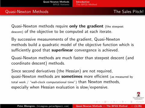
Quasi-Newton Methods The Sales Pitch!
Quasi-Newton methods require only the gradient (like steepest
descent) of the objective to be computed at each iterate.
By successive measurements of the gradient, Quasi-Newtonmethods build a quadratic model of the objective function which issufficiently good that superlinear convergence is achieved.
Quasi-Newton methods are much faster than steepest descent (andcoordinate descent) methods.
Since second derivatives (the Hessian) are not required,quasi-Newton methods are sometimes more efficient (as measured by
total work / “wall-clock computational time”) than Newton methods,especially when Hessian evaluation is slow/expensive.
Peter Blomgren, 〈[email protected]〉 Quasi-Newton Methods — The BFGS Method — (3/26)

Quasi-Newton MethodsBFGS Variants
IntroductionThe BFGS Method
The BFGS Method: Introduction 1 of 3
The BFGS method is named for its discoverers:Broyden-Fletcher-Goldfarb-Shanno, and is the most popularquasi-Newton method.
We derive the DFP (a close relative; named afterDavidon-Fletcher-Powell) and BFGS methods; and look atsome properties and practical implementation details.
The derivation starts with the quadratic model
mk(p) = f (xk) +∇f (xk)T p+
1
2pTBk p
at the current iterate xk . Bk is a symmetric positive definitematrix (model Hessian) that will be updated in every iteration.
Peter Blomgren, 〈[email protected]〉 Quasi-Newton Methods — The BFGS Method — (4/26)
Quasi-Newton MethodsBFGS Variants
IntroductionThe BFGS Method
The BFGS Method: Introduction Standard Stuff 2 of 3
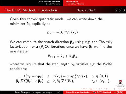
Given this convex quadratic model, we can write down theminimizer pk explicitly as
pk = −B−1k ∇f (xk).
We can compute the search direction pk using e.g. the Choleskyfactorization, or a (P)CG-iteration; once we have pk we find thenew iterate:
xk+1 = xk + αk pk ,
where we require that the step length αk satisfies e.g. the Wolfeconditions:
f (xk + αpk) ≤ f (xk) + c1αpTk ∇f (x), c1 ∈ (0, 1)
pTk ∇f (xk + αpk) ≥ c2pTk ∇f (xk), c2 ∈ (c1, 1).
Peter Blomgren, 〈[email protected]〉 Quasi-Newton Methods — The BFGS Method — (5/26)
Quasi-Newton MethodsBFGS Variants
IntroductionThe BFGS Method
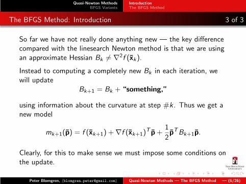
The BFGS Method: Introduction 3 of 3
So far we have not really done anything new — the key differencecompared with the linesearch Newton method is that we are usingan approximate Hessian Bk 6= ∇
2f (xk).
Instead to computing a completely new Bk in each iteration, wewill update
Bk+1 = Bk + “something,”
using information about the curvature at step #k . Thus we get anew model
mk+1(p) = f (xk+1) +∇f (xk+1)T p+
1
2pTBk+1p.
Clearly, for this to make sense we must impose some conditions onthe update.
Peter Blomgren, 〈[email protected]〉 Quasi-Newton Methods — The BFGS Method — (6/26)
Quasi-Newton MethodsBFGS Variants
IntroductionThe BFGS Method
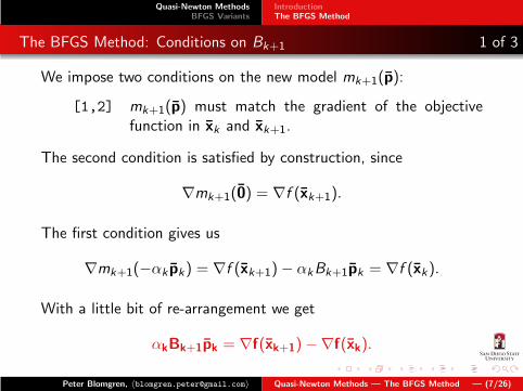
The BFGS Method: Conditions on Bk+1 1 of 3
We impose two conditions on the new model mk+1(p):
[1,2] mk+1(p) must match the gradient of the objectivefunction in xk and xk+1.
The second condition is satisfied by construction, since
∇mk+1(0) = ∇f (xk+1).
The first condition gives us
∇mk+1(−αk pk) = ∇f (xk+1)− αkBk+1pk = ∇f (xk).
With a little bit of re-arrangement we get
αkBk+1pk = ∇f(xk+1)−∇f(xk).
Peter Blomgren, 〈[email protected]〉 Quasi-Newton Methods — The BFGS Method — (7/26)
Quasi-Newton MethodsBFGS Variants
IntroductionThe BFGS Method
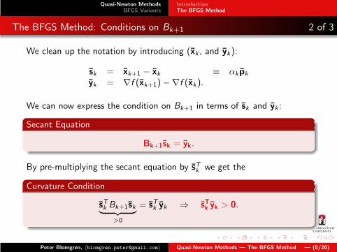
The BFGS Method: Conditions on Bk+1 2 of 3
We clean up the notation by introducing (xk , and yk):
sk = xk+1 − xk ≡ αk pkyk = ∇f (xk+1)−∇f (xk).
We can now express the condition on Bk+1 in terms of sk and yk :
Secant Equation
Bk+1sk = yk.
By pre-multiplying the secant equation by sTk we get the
Curvature Condition
sTk Bk+1sk︸ ︷︷ ︸
>0
= sTk yk ⇒ sTk yk > 0.
Peter Blomgren, 〈[email protected]〉 Quasi-Newton Methods — The BFGS Method — (8/26)
Quasi-Newton MethodsBFGS Variants
IntroductionThe BFGS Method
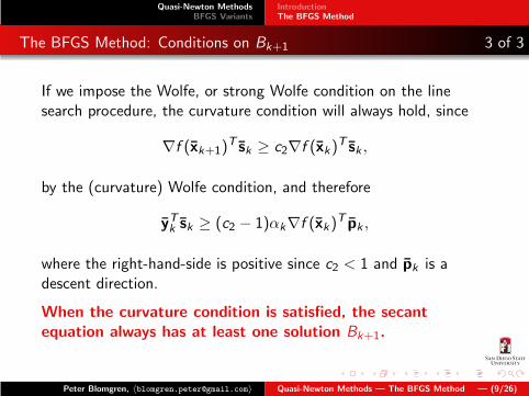
The BFGS Method: Conditions on Bk+1 3 of 3
If we impose the Wolfe, or strong Wolfe condition on the linesearch procedure, the curvature condition will always hold, since
∇f (xk+1)T sk ≥ c2∇f (xk)
T sk ,
by the (curvature) Wolfe condition, and therefore
yTk sk ≥ (c2 − 1)αk∇f (xk)T pk ,
where the right-hand-side is positive since c2 < 1 and pk is adescent direction.
When the curvature condition is satisfied, the secantequation always has at least one solution Bk+1.
Peter Blomgren, 〈[email protected]〉 Quasi-Newton Methods — The BFGS Method — (9/26)
Quasi-Newton MethodsBFGS Variants
IntroductionThe BFGS Method
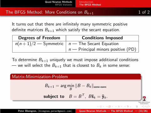
The BFGS Method: More Conditions on Bk+1 1 of 2
It turns out that there are infinitely many symmetric positivedefinite matrices Bk+1 which satisfy the secant equation.
Degrees of Freedom Conditions Imposed
n(n + 1)/2 — Symmetric n — The Secant Equationn — Principal minors positive (PD)
To determine Bk+1 uniquely we must impose additional conditions— we will select the Bk+1 that is closest to Bk in some sense:
Matrix-Minimization-Problem
Bk+1 = argminB‖B − Bk‖some-norm
subject to B = BT , B sk = yk .
Peter Blomgren, 〈[email protected]〉 Quasi-Newton Methods — The BFGS Method — (10/26)
Quasi-Newton MethodsBFGS Variants
IntroductionThe BFGS Method
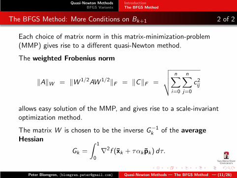
The BFGS Method: More Conditions on Bk+1 2 of 2
Each choice of matrix norm in this matrix-minimization-problem(MMP) gives rise to a different quasi-Newton method.
The weighted Frobenius norm
‖A‖W = ‖W 1/2AW 1/2‖F = ‖C‖F =
√√√√
n∑
i=0
n∑
j=0
c2ij
allows easy solution of the MMP, and gives rise to a scale-invariantoptimization method.
The matrix W is chosen to be the inverse G−1k of the average
Hessian
Gk =
∫ 1
0∇2f (xk + ταk pk) dτ.
Peter Blomgren, 〈[email protected]〉 Quasi-Newton Methods — The BFGS Method — (11/26)
Quasi-Newton MethodsBFGS Variants
IntroductionThe BFGS Method
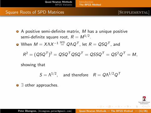
Square Roots of SPD Matrices [Supplemental]
A positive semi-definite matrix, M has a unique positivesemi-definite square root, R = M1/2.
When M = XΛX−1 SPD= QΛQT , let R = QSQT , and
R2 = (QSQT )2 = QSQTQSQT = QSSQT = QS2QT = M,
showing that
S = Λ1/2, and therefore R = QΛ1/2QT
∃ other approaches.
Peter Blomgren, 〈[email protected]〉 Quasi-Newton Methods — The BFGS Method — (12/26)
Quasi-Newton MethodsBFGS Variants
IntroductionThe BFGS Method
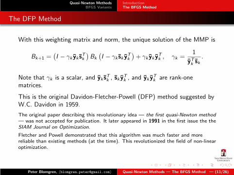
The DFP Method
With this weighting matrix and norm, the unique solution of the MMP is
Bk+1 =(I − γk yk s
Tk
)Bk
(I − γk sk y
Tk
)+ γk yk y
Tk , γk =
1
yTk sk.
Note that γk is a scalar, and yk sTk , sk y
Tk , and yk y
Tk are rank-one
matrices.
This is the original Davidon-Fletcher-Powell (DFP) method suggested byW.C. Davidon in 1959.
The original paper describing this revolutionary idea — the first quasi-Newton method
— was not accepted for publication. It later appeared in 1991 in the first issue the theSIAM Journal on Optimization.
Fletcher and Powell demonstrated that this algorithm was much faster and morereliable than existing methods (at the time). This revolutionized the field of non-linearoptimization.
Peter Blomgren, 〈[email protected]〉 Quasi-Newton Methods — The BFGS Method — (13/26)
Quasi-Newton MethodsBFGS Variants
IntroductionThe BFGS Method
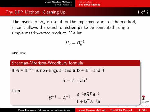
The DFP Method: Cleaning Up 1 of 2
The inverse of Bk is useful for the implementation of the method,since it allows the search direction pk to be computed using asimple matrix-vector product. We let
Hk = B−1k
and use
Sherman-Morrison-Woodbury formula
If A ∈ Rn×n is non-singular and a, b ∈ R
n, and if
B = A+ abT
then
B−1 = A−1 −A−1abTA−1
1 + bTA−1a.
Peter Blomgren, 〈[email protected]〉 Quasi-Newton Methods — The BFGS Method — (14/26)

Quasi-Newton MethodsBFGS Variants
IntroductionThe BFGS Method
The DFP Method: Cleaning Up 2 of 2
With a little bit of linear algebra we end up with
Hk+1 = Hk −Hk yk y
Tk Hk
yTHk yk︸ ︷︷ ︸
Update#1
+sk s
Tk
yTk sk︸ ︷︷ ︸
Update#2
.
Both the update terms are rank-one matrices; so that Hk
undergoes a rank-2 modification in each iteration.
This is the fundamental idea of quasi-Newton updating:instead of recomputing the matrix (-inverse) from scratch eachtime around, we apply a simple modification which combines themore recently observed information about the objective withexisting knowledge embedded in the current Hessianapproximation.
Peter Blomgren, 〈[email protected]〉 Quasi-Newton Methods — The BFGS Method — (15/26)
Quasi-Newton MethodsBFGS Variants
IntroductionThe BFGS Method
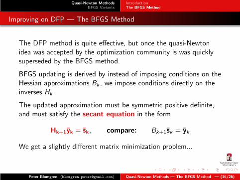
Improving on DFP — The BFGS Method
The DFP method is quite effective, but once the quasi-Newtonidea was accepted by the optimization community is was quicklysuperseded by the BFGS method.
BFGS updating is derived by instead of imposing conditions on theHessian approximations Bk , we impose conditions directly on theinverses Hk .
The updated approximation must be symmetric positive definite,and must satisfy the secant equation in the form
Hk+1yk = sk, compare: Bk+1sk = yk
We get a slightly different matrix minimization problem...
Peter Blomgren, 〈[email protected]〉 Quasi-Newton Methods — The BFGS Method — (16/26)
Quasi-Newton MethodsBFGS Variants
IntroductionThe BFGS Method
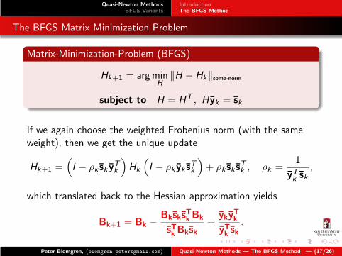
The BFGS Matrix Minimization Problem
Matrix-Minimization-Problem (BFGS)
Hk+1 = argminH‖H − Hk‖some-norm
subject to H = HT , H yk = sk
If we again choose the weighted Frobenius norm (with the sameweight), then we get the unique update
Hk+1 =(
I − ρk sk yTk
)
Hk
(
I − ρk yk sTk
)
+ ρk sk sTk , ρk =
1
yTk sk,
which translated back to the Hessian approximation yields
Bk+1 = Bk −Bksks
TkBk
sTkBksk+
ykyTk
yTk sk.
Peter Blomgren, 〈[email protected]〉 Quasi-Newton Methods — The BFGS Method — (17/26)
Quasi-Newton MethodsBFGS Variants
IntroductionThe BFGS Method
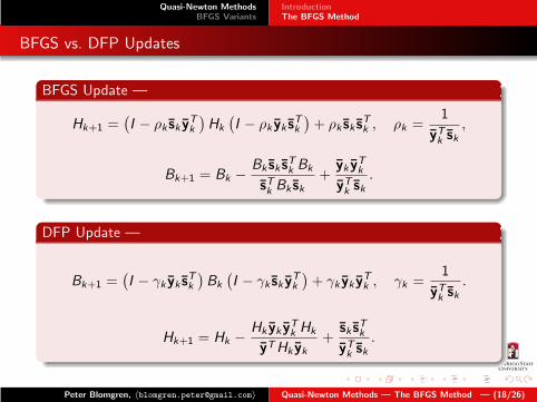
BFGS vs. DFP Updates
BFGS Update —
Hk+1 =(I − ρk sk y
Tk
)Hk
(I − ρk yk s
Tk
)+ ρk sk s
Tk , ρk =
1
yTk sk,
Bk+1 = Bk −Bk sk s
Tk Bk
sTk Bk sk+
yk yTk
yTk sk.
DFP Update —
Bk+1 =(I − γk yk s
Tk
)Bk
(I − γk sk y
Tk
)+ γk yk y
Tk , γk =
1
yTk sk.
Hk+1 = Hk −Hk yk y
Tk Hk
yTHk yk+
sk sTk
yTk sk.
Peter Blomgren, 〈[email protected]〉 Quasi-Newton Methods — The BFGS Method — (18/26)
Quasi-Newton MethodsBFGS Variants
IntroductionThe BFGS Method
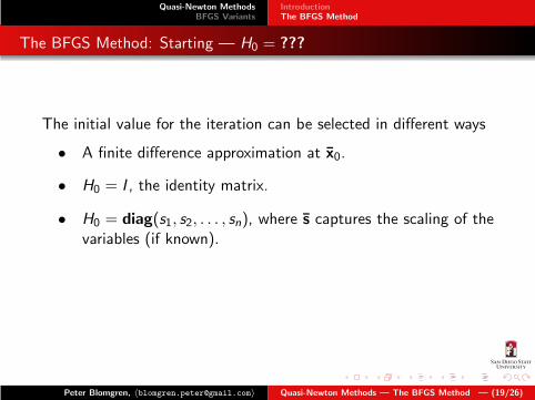
The BFGS Method: Starting — H0 = ???
The initial value for the iteration can be selected in different ways
• A finite difference approximation at x0.
• H0 = I , the identity matrix.
• H0 = diag(s1, s2, . . . , sn), where s captures the scaling of thevariables (if known).
Peter Blomgren, 〈[email protected]〉 Quasi-Newton Methods — The BFGS Method — (19/26)
Quasi-Newton MethodsBFGS Variants
IntroductionThe BFGS Method
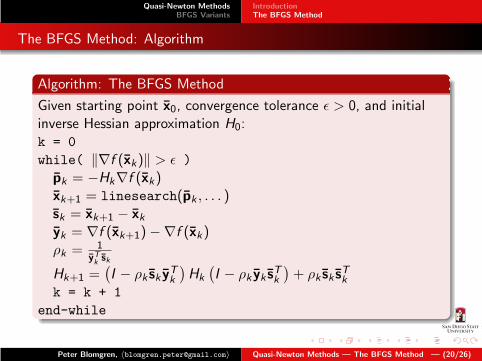
The BFGS Method: Algorithm
Algorithm: The BFGS Method
Given starting point x0, convergence tolerance ǫ > 0, and initialinverse Hessian approximation H0:k = 0
while( ‖∇f (xk)‖ > ǫ )
pk = −Hk∇f (xk)xk+1 = linesearch(pk , . . . )sk = xk+1 − xkyk = ∇f (xk+1)−∇f (xk)ρk = 1
yTksk
Hk+1 =(I − ρk sk y
Tk
)Hk
(I − ρk yk s
Tk
)+ ρk sk s
Tk
k = k + 1
end-while
Peter Blomgren, 〈[email protected]〉 Quasi-Newton Methods — The BFGS Method — (20/26)
Quasi-Newton MethodsBFGS Variants
IntroductionThe BFGS Method
The BFGS Method: Summary
The cost per iteration is
• O(n2) arithmetic operations
• function evaluation
• gradient evaluation
The convergence rate is
• Super-linear
Newton’s method converges quadratically, but the cost periteration is higher — it requires the solution of a linear system. Inaddition Newton’s method requires the calculation of secondderivatives whereas the BFGS method does not.
Peter Blomgren, 〈[email protected]〉 Quasi-Newton Methods — The BFGS Method — (21/26)
Quasi-Newton MethodsBFGS Variants
IntroductionThe BFGS Method
The BFGS Method: Stability and Self-Correction 1 of 2
If at some point ρk = 1/yTk sk becomes large, i.e. yTk sk ∼ 0, thenfrom the update formula
Hk+1 =(
I − ρk sk yTk
)
Hk
(
I − ρk yk sTk
)
+ ρk sk sTk
we see that Hk+1 becomes large.
If for this, or some other, reason Hk becomes a poor approximationof
[∇2f (xk)
]−1
for some k , is there any hope of correcting it?
It has been shown that the BFGS method has self-correctingproperties. — If Hk incorrectly estimates the curvature of theobjective function, and if this estimate slows down the iteration,then the Hessian approximation will tend to correct itself within afew steps.
Peter Blomgren, 〈[email protected]〉 Quasi-Newton Methods — The BFGS Method — (22/26)
Quasi-Newton MethodsBFGS Variants
IntroductionThe BFGS Method
The BFGS Method: Stability and Self-Correction 2 of 2
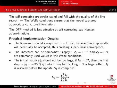
The self-correcting properties stand and fall with the quality of the linesearch! — The Wolfe conditions ensure that the model capturesappropriate curvature information.
The DFP method is less effective at self-correcting bad Hessianapproximations.
Practical Implementation Details:
• The linesearch should always test α = 1 first, because this step lengthwill eventually be accepted, thus creating super-linear convergence.
• The linesearch can be somewhat “sloppy:” c1 = 10−4 and c2 = 0.9are commonly used values in the Wolfe conditions.
• The initial matrix H0 should not be too large, if H0 = βI , then the firststep is p0 = −β∇f (x0) which may be too long if β is large, often H0
is rescaled before the update H1 is computed:
H0 ←yTk skyTk yk
I .
Peter Blomgren, 〈[email protected]〉 Quasi-Newton Methods — The BFGS Method — (23/26)
Quasi-Newton MethodsBFGS Variants
Limited-memory BFGS
L-BFGS
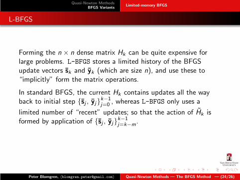
Forming the n × n dense matrix Hk can be quite expensive forlarge problems. L-BFGS stores a limited history of the BFGSupdate vectors sk and yk (which are size n), and use these to“implicitly” form the matrix operations.
In standard BFGS, the current Hk contains updates all the wayback to initial step {sj , yj}
k−1j=0 , whereas L-BFGS only uses a
limited number of “recent” updates; so that the action of Hk isformed by application of {sj , yj}
k−1j=k−m
.
Peter Blomgren, 〈[email protected]〉 Quasi-Newton Methods — The BFGS Method — (24/26)
Quasi-Newton MethodsBFGS Variants
Limited-memory BFGS
L-BFGS ”Two Loop Recursion”
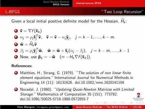
Given a local initial positive definite model for the Hessian, Hk :
1 v = ∇f (xk)
2 αj = ρj sTj v, v = v − αj yj , j = k − 1, . . . , k −m.
3 w = Hk v
4 βj = ρj yTj w, w = w + sj(αj − βj), j = k −m, . . . , k − 1
5 Now, use pk = −w (≈ −Hk∇f (xk)).
References:
1 Matthies, H.; Strang, G. (1979). ”The solution of non linear finite
element equations.” International Journal for Numerical Methods inEngineering 14 (11): 16131626. doi:10.1002/nme.1620141104
2 Nocedal, J. (1980). ”Updating Quasi-Newton Matrices with Limited
Storage.” Mathematics of Computation 35 (151): 773782.doi:10.1090/S0025-5718-1980-0572855-7
Peter Blomgren, 〈[email protected]〉 Quasi-Newton Methods — The BFGS Method — (25/26)
Quasi-Newton MethodsBFGS Variants
Limited-memory BFGS
Index
matrix-minimization-problemBGFS, 17DFP, 10
Reference(s):
D1991 Davidon, William C. ”Variable metric method for minimization.” SIAM Journal on Optimization 1, no. 1(1991): 1-17.
MS1979 Matthies, H.; Strang, G. (1979). ”The solution of non linear finite element equations.” InternationalJournal for Numerical Methods in Engineering 14 (11): 16131626. doi:10.1002/nme.1620141104
N1980 Nocedal, J. (1980). ”Updating Quasi-Newton Matrices with Limited Storage.” Mathematics ofComputation 35 (151): 773782. doi:10.1090/S0025-5718-1980-0572855-7
Peter Blomgren, 〈[email protected]〉 Quasi-Newton Methods — The BFGS Method — (26/26)