NUMERICAL MULTISCALE METHODS FOR COUPLEDOSCILLATORS

GIL ARIEL, BJORN ENGQUIST, AND RICHARD TSAI

ABSTRACT. A multiscale method for computing the effective slow behavior ofa system of weakly coupled general oscillators is presented. The oscillators maybe either in the form of a periodic solution or a stable limit cycle. Furthermore,the oscillators may be in resonance with one another and thereby generate somehidden slow dynamics. The proposed method relies on correctly tracking a set ofslow variables that is sufficient to approximate any variable and functional that areslow under the dynamics of the ODE. The technique is more efficient than exist-ing methods and its advantages are demonstrated with examples. The algorithmfollows the framework of the heterogeneous multiscale method.

1. INTRODUCTION

Ordinary differential equations (ODEs) with highly oscillatory periodic solutionsprove to be a challenging field of research from both the analytic and numericalpoints of view [15, 16]. Several different numerical approaches have been sug-gested, each appropriate to some class of ODEs. Dahlquist laid down the funda-mental work for designing linear multistep methods [4, 5, 6, 7] and studied theirstability properties. Stiff problems with fast transients can be optimally solved byimplicit schemes [4, 18, 22]. The Chebyshev methods [1, 24] as well as the pro-jective integrator approach [13] provide stable and explicit computational strategiesfor this class of problems in general. Chebyshev methods are also efficient withproblems that have a cascade of different scales which are not necessarily wellseparated. For harmonic oscillatory problems, traditional numerical approaches at-tempt to either filter out or fit fast, ε-scale oscillations to some known functions inorder to reduce the complexity, e.g. [12, 23, 30], or use some notion of Poincarémap to determine slow changes in the orbital structure [14, 27]. A general class ofapproaches aiming at Hamiltonian systems are geometric integration schemes thatpreserve a discrete version of certain invariance. We refer the readers to [17] and[25] for more extensive list of literature. Many of the schemes specialized for finitedimensional mechanical systems can be conveniently derived from the view pointof variational integrator; see the review paper [26]. In certain applications, specialconsiderations are given to the expensive cost of evaluating non-local potential inlarge systems, see e.g. the impulse method and its derivatives [25]. For a recentreview on numerical methods for highly oscillatory systems see [3].

1

In this paper, we refer to a pair (x, y) as an oscillator if the trajectory (x(t), y(t)) iseither periodic or approaches a stable periodic limit cycle. The period of anoscilla-tor is denoted T0. One typical example is the Van der Pol oscillator [31],

(1.1) x = −x+ ν(1− x2)x,

for some ν > 0. Equation (1.1) has a unique and stable limit cycle that tends tothe circle x2 + x2 = 4 in the limit ν → 0. Another type of oscillators arise when asystem of ODEs has a family of periodic solutions.

In this paper we propose a numerical multiscale scheme for the initial value prob-lems in which different oscillators are coupled weakly. The period of each oscilla-tion is taken to be proportional to a small parameters ε� 1. The coupling producessignificant influence to the system in a longer time scale. We are particularly in-terested in resonance or synchronization effects. Consequently, we assume that thefrequencies of the uncoupled oscillators are commensurable.

Let {(xk, yk)}lk=1 denote a set of l oscillators with xk, yk ∈ R. We consider ODEsystems in singular perturbation form

(1.2) εx = f(x) + εg(x), x(0) = x0,

where 0 < ε ≤ ε0 and x = (x1, y1, x2, y2, . . . , xl, yl). It is further assumed that thesolution of (1.2) remains in a domain D0 ⊂ R2l, that is bounded independent of εfor all t ∈ [0, T ], T <∞ and independent of ε. For fixed ε and initial condition x0,the solution of (1.2) is denoted x(t; ε,x0). For brevity we will write x(t) wheneverit is clear what the values for ε and x0 are. On short time scales of order ε, theterm εg(x) can be neglected. However, on longer time scales which are independentof ε, this perturbation may accumulate to an important contribution that cannot beignored.

One of the main difficulties in numerical integration of (1.2) using explicit meth-ods is that stability and accuracy requirements severely restrict the usable step size.This generally implies that the computational complexity for integrating (1.2) overa time T is at least of the order of ε−1. This is the motivation for multiscale nu-merical schemes that take advantage of the separation between time scales in theproblem. The new schemes proposed in this paper generalize those in [2] to sys-tems of nonlinear oscillators. The computational cost of our proposed schemes aresublinear in the frequency of the oscillators. Furthermore, it can be applied to prob-lems for which specialized algorithms such as the exponential integrators [17, 20]do not apply, or do not yield efficient approximations.

The various types of oscillators make a general method difficult. As a recourse,we first describe the main idea behind our algorithm and then apply it to severalexamples involving different types of oscillators. An important component in ourapproach is to identify a set of functions of x that are slow with respect to the dy-namics of (1.2), i.e., the time derivatives of these functions are uniformly boundedwith a constant that is independent of ε along the trajectories of (1.2). We clas-sify these functions as the square amplitudes and the relative phases between the

2

oscillators. We generally refer to them as the slow variables of the system. TheODE (1.2) is then integrated using the framework of the heterogeneous multiscalemethod (HMM) [9, 10, 11] — a Macro-solver integrates the effective, but gener-ally unknown evolution equation for the slow variables under the dynamics of (1.2),where the rate of change for these slow variables are computed by a micro-solverthat integrates the full ODE (1.2) for short time segments.

For convenience, Section 2 reviews the main results and algorithm proposed in [2]and [11]. Section 3 describes a method for applying the HMM algorithm to systemsof weakly coupled oscillators. Several examples are studies in Section 4 includingharmonic Volterra-Lotka and relaxation oscillators. The Volterra-Lotka exampleadmits a family of periodic solutions that correspond to some constants of motion.On the other hand, in the relaxation oscillator example trajectories rapidly approacha stable limit cycle. We conclude in Section 5.

2. THE HMM SCHEME

In this section we summarize the main results of [2] and [11]. We begin by analyz-ing how the slow aspects of a multiscale ODE can be identified and separated fromthe fast one by using a convenient system of coordinates. Then, an algorithm forapproximating and evoling these slow aspects is reviewed. The algorithm followsthe framework of the Heterogeneous Multiscale Methods [10].

2.1. Fast and slow dynamics. We study the long time properties of (1.2) by sepa-rating the fast and slow constituents of the dynamics and investigating the interac-tions between these constituents and the collective effective behavior. We say thata real valued smooth function (variable) α(x) is slow with respect to (1.2) if thereexists a non-empty open set A ⊂ Rd such that

(2.1) maxx0∈A,t∈I,ε∈(0,ε0]

∣∣∣∣ ddtα(x(t; ε,x0))

∣∣∣∣ ≤ C0,

where C0 is a constant that is independent of ε and I = [0, T ]. Otherwise, α(x) issaid to be fast. Similarly, we say that a quantity or constant is of order one if it isbounded independent of ε in A. We typically consider functions that are indepen-dent of ε. For integrable hamiltonian systems, the action variables are indeed slowvariables.

Of course, any function of slow variables is also slow. Therefore, it is reason-able to look for variables which are functionally independent, i.e., a vector of slowvariables ξ = (ξ1(x), . . . , ξr(x)) such that ∇ξ1(x), . . . ,∇ξr(x) are linearly inde-pendent in A. Since r is bounded by the dimension, d, it is useful to look at aset with a maximal number of functinally independent slow variables. Augmentingthe slow variables with d − r fast ones z = (z1, . . . , zd−r) such that ∂(ξ, z)/∂x isnon-singular in A, one obtains a local coordinate systems, i.e., a chart of the statesspace. We will refer to a chart in which a maximal number of coordinates is slow

3

as a maximal slow chart for A with respect to the ODE (1.2). Covering the set D0

by maximal slow charts we obtain a maximal slow atlas for D0.

A second type of slow behavior, referred to as slow observables, are integrals of thetrajectories. For example, for any integrable function α(x, t), the integral

(2.2) α(t) =

∫ t

0

α(x(s), s)ds

is slow since |dα/dt| ≤ C for some constant C > 0 Additional slow observablescan be obtained using convolution with a compactly supported kernels, as explainedat the end of this Section.

The difficulty is that it is often not clear a priori which of the slow variables andobservables are of interest. For this reason, we take a wide approach and requirethat our algorithm approximates all variables and observables which are slow withrespect to the ODE. To see how it is possible, let (ξ, φ) ∈ Rd denote a slow chartwith slow coordinates ξ ∈ Rr and let α(x) : Rd → R a slow variable. Then, bythe maximality of the chart, there exists a function α : Rr → Rd such that α(x) =α(ξ(x)), otherwise, α(x) can be added as an additional coordinate. So if the valuesof ξ along the trajectories of (1.2) is accurately approximated, the values of anyother smooth slow variables along the trajectories are automatically approximated.Furthermore, it is not necessary to know α since all points x which correspond tothe same ξ yield the same value of α(x). In [2] we prove that approximation of ξ isalso sufficient to approximate all slow observables of the types described above.

Construction of our multiscale algorithm takes three stages. The first required iden-tification of a maximal slow chart or atlas (ξ, φ) which needs to be defined in aneighborhood of the trajectory. Locally, any coordinates system on a manifold thatis perpendicular to f(x) can serve as a maximal slow chart. However, extending achart to include the full trajectory is more difficult. This is done in [2] for the casein which the leading order term in (1.2) is linear, f(x) = Ax. The main purpose ofthis paper is offer a similar construction for some cases in which the solutions arestill periodic in nature although f(x) may not be linear.

The second stage is to establish the existence of an effective evolution equation forthe slow variables ξ(x(t)) under the flow of (1.2). In all the examples discussesin this paper, the fast coordinate will be taken as a fast rotation of the unit circlewith constant velocity, i.e., φ ∈ S1. This case is quite general since many weaklyperturbed integrable systems in resonance fall into this category. Then, an aver-aging principle can be used to prove [2, 29] that for small ε, ξ(x(t; ε,x0)) is wellapproximated in I by an effective equation of the form

(2.3) ξ = F (ξ), ξ(0) = ξ(x0).

The requirement that (ξ, φ) is a maximal slow chart is critical for the derivationof (2.3). Without it, there is no guaranty that the right hand side of the averagedequation does not depend on additional slow variables which may be hidden orunknown.

4

The effective equation (2.3) may not be available as an explicit formula. Instead, theidea behind the HMM algorithm is to evaluate F (ξ) by numerical solutions of theoriginal ODE (1.2) on significantly reduced time intervals. In this way, the HMMalgorithm approximates an assumed effective equation whose form is typically un-known. This strategy is advantageous if F (ξ) can be approximated efficiently. Thethird step of the process is to construct such an algorithm. This is explained belowin Section 2.2.

In [2] we present both analytic and numerical methods for finding such a chart in aneighborhood of the trajectories in the case in which f(x) is linear, i.e., f(x) = Axand A is a diagonalizable matrix whose eigenvalues have non-positive real parts.It is then proven that the slow atlas can be described using a single chart whichconsists of the following slow variables:

• Slow variables that correspond to a basis of the Null space of A.• Amplitudes of oscillators (or rather square of), which are quadratic func-

tions of x.• The relative phase between each pair of oscillators which correspond to

some specific coupling of different oscillators through initial conditions. Ifthe ratio between the frequencies of two oscillators is a rational number,then this relative phase can be defined by a specific polynomial in x.

A simple example is the following system described by

(2.4) εx =

0 1 0 0 0−1 0 0 0 00 0 0 2 00 0 −2 0 00 0 0 0 0

x + εg(x),

where x = (x1, y1, x2, y2, x3). Here (x1, y1) and (x2, y2) are harmonic oscillatorswith frequencies 1/2π and 1/π, respectively. One verifies that x3 is slow and thatthe square amplitudes, I1 = x2

1 + y21 and I2 = x2

2 + y22 , are slow. In addition, the

cubic polynomial J1 = x21x2 + 2x1y1y2 − y2

1x2 is also slow. This is verified bydifferentiating J1(x(t)) with respect to time. The polynomial J1 is related to therelative phase between the two harmonic oscillators, a quantity that varies slowly intime.

The main purpose of this paper is to extend these ideas to a wider class of ODEs.We find that the components of slow charts can be interpreted as some generalizedconcepts of amplitudes and relative phases. A few typical examples, for which thisprogram can be carried through, are analyzed in the following sections.

2.2. The algorithm. Suppose ξ = (ξ1(x), . . . , ξr(x)) are the slow variables in aslow atlas for (1.2). The system is integrated using a two level algorithm, eachlevel corresponding to a different time scale. The first is a Macro-solver, whichintegrates the effective equation (2.3) for the slow variables ξ. The second level is a

5

micro-solver that is invoked whenever the Macro-solver needs an estimate of F (ξ).The micro-solver computes a short time solution of (1.2) using suitable initial data.Then, the time derivative of ξ is approximated by

(2.5) ξ(t) ∼ 〈ξ(t)〉η =

∫ η/2

−η/2ξ(t+ τ)Kη(t+ η/2− τ)dτ,

where, Kη(·) denotes a smooth averaging kernel with support on [−η/2, η/2]. Notethat ξ is not necessarily slow. However, it is bounded independent of ε. The prop-erties of averaging with respect to a kernel will be reviewed shortly.

Once time derivatives are approximated, the system needs to be evolved in a waythat is consistent with (2.5). For example, a step x(t+H) = x(t) + ∆x, correct tosecond order in H , is to take the least squares solution of the linear system

∆x · ∇ξk(x(t)) = H〈ξk(t)〉η, k = 1, . . . , r.

Higher order methods are explained in [2].

To better explain the algorithm, denote the Macro-solver sample times by t0, . . . , tN ,N = T/H , and its output at corresponding times by x0, . . . ,xN . At the n-th Macro-step, the micro-solver can be implemented using any scheme with step-size h andinitial condition x(tn) = xn. It integrates the full ODE both backwards and for-ward in time to approximate the solution in [tn − η/2, tn + η/2]. The structure ofthe algorithm, depicted in Figure 2.1, is as follows.

(1) Initial conditions: x(0) = x0 and n = 0.(2) Force estimation:

(a) micro-simulation: Solve (1.2) in [tn − η/2, tn + η/2] with initial con-ditions x(tn) = xn.

(b) Averaging: approximate ξk(tn) by 〈ξk(tn)〉η.(3) Macro-step (forward Euler example):

xn+1 = xn + HFn, where Fn is the least squares solution of the linearsystem

Fn · ∇ξk(xn) = 〈ξk(tn)〉η, k = 1 . . . r

(4) n = n+ 1. Repeat steps (2) and (3) to time ε−1T .

The averaged time derivative of ξk, 〈ξk〉η, can be calculated using either the chainrule as ξk = ∇ξk · x = ∇ξk · (f(x) + εg(x)), or using integration by parts. Thescheme described above can be generalized to Macro-solvers with higher order ac-curacy.

Let K(·) denote a smooth kernel function with support on [−1, 1] with unit mass,∫ 1

−1K(τ)dτ = 1, and zero average,

∫ 1

−1K(τ)τdτ = 0. For simplicity, we assume

that K(·) is symmetric with respect to its mid-point. For example, the followingsmooth exponential kernel was found useful:

(2.6) K(t) = Z−1 exp

(−5

4

1

(t− 1)(t+ 1)

),

6

hx(0)

x

ξ

η

micro−solver

Macro−solverH

FIGURE 2.1. The cartoon depicts the time steps taken by the HMMscheme. At the n-th macro step, a micro-solver with step size hintegrates (1.2) to approximate x(t) in a time segment [tn−η/2, tn+η/2]. This data is used to calculate 〈ξ(x(t))〉η. Then, the Macro-solver takes a big step of size HFn, where Fn is consistent with〈ξk〉η, i.e., Fn ·∇ξk = 〈ξk〉η for all slow variables ξk in the maximallyslow chart.

for t ∈ [−1, 1] and zero otherwise. Here, Z is a normalization constant. For η > 0let,

(2.7) Kη(τ) =1

2ηK(

1

2ητ).

We will take η to be ε dependent such that ε < η � 1. The convolution of a functiona(t) with Kη is denoted as (recall (2.5))

(2.8) 〈a(t)〉η =

∫ η/2

−η/2a(t+ τ)Kη(t+ η/2− τ)dτ.

Typically, the fast dynamics in equations such as (1.2) is one of two types. Thefirst consists of modes that are attracted to a low dimensional manifold in ε-timescale. These modes are referred to as transient or dissipative modes and will notbe discussed in this paper. The second type consists of oscillators with constantor slowly changing frequencies. Averaging of oscillatory modes filters out highfrequency oscillations. The errors introduced by the averaging are estimated in [2].Asymmetric kernels can also be used in order to obtain an improved accuracy.

Finally, the stability of the algorithm is related to integration of the approximateeffective equation for the slow variables, ξ = 〈ξ(x(t))〉η using the Macro-solver ofchoice. Additional details can be found in [10] and [11].

3. SLOW CHARTS FOR COUPLED OSCILLATORS

In this section we outline a method for constructing slow charts for weakly coupledoscillators. A few specific examples are detailed in the following sections. For

7

simplicity, we consider a system of two planar oscillators, z, γ ∈ R2, of the form

(3.1)

{εz = f(z),

εγ = g(γ),

where the trajectory (z(t; z0), γ(t; γ0)) ∈ R2 × R2 is either periodic or approachesa stable periodic limit cycle. In addition, consider the perturbed systems

(3.2)

{ε ˙z = fε(z, γ) = f(z) + εh(z, γ)

ε ˙γ = gε(z, γ) = g(γ) + εk(z, γ).

We would like to study the effective behavior of the coupled system (3.2), in partic-ular the effective influence of the perturbative coupling. This could be done usingsome generalized notions of amplitude and relative phase to form slow charts in thestate space.

Suppose that, in the limit ε→ 0, the trajectory of each oscillator approaches a stableperiodic limit cycle. Two possibilities may occur [19, 21, 29, 32]. First, the limitcycle may be attractive, in which case any all trajectories that start close enough willbe asymptotically close to it. Second, there may a continuous one parameter familyof periodic orbits. In either case, one can often use this parameter to describe thecloseness of the trajectory to the limit cycle [19]. In the first case, the parameter is adissipative, “fast” variable. In the second case it is slow. We think of this parameteras some generalized amplitude, in the sense that it identifies the periodic limit cycleof the oscillators. See, for example the discussion on the Van der Pol oscillatorin [19]. The generalized amplitudes of the two oscillators are denoted I1 and I2,respectively.

3.1. Slowly changing observables along the trajectories. We observe that alongeach trajectory of (3.2), a slow variable defines a slowly changing quantity ϑ. First,consider the unperturbed equation (3.1) and a slow variable α(z, γ). We denote

(3.3)d

dtα(z(t), γ(t)) =

1

ε(∇zα|z(t),γ(t) · f + ε∇γα|z(t),γ(t) · g) =: φf,gα (t; z0, γ0),

where ∇z and ∇γ denote the gradients with respect to z and γ, respectively. Be-cause α(z, γ) is slow, we have that |φf,gα (t; z0, γ0)| ≤ C1. If this bound is valid for0 < ε ≤ ε0, then∇zα · f = 0. Next, consider the perturbed equation (3.2). We maydirectly consider integrating a slow observable ϑ(t) satisfying

(3.4)d

dtϑ = φfε,gεα (t; y0), ϑ(0) = ϑ0.

Notice that

φfε,gεα =1

ε(∇zα|z(t),γ(t) · fε + ε∇γα|z(t),γ(t) · gε) = ∇zα|z(t),γ(t) ·h+∇γα|z(t),γ(t) ·k.

Hence, ϑ(t) is slowly varying on a O(1) time scale.8

3.2. Relative phase defined by time. We first consider the unperturbed system(3.1). Time may be used to defined what the phase of the trajectory of an oscillatormeans. Suppose for the moment that there exist two functions τz(z) and τγ(γ) suchthat ετz(z(t)) = t+ c0 and ετγ(γ(t)) = t+ c1. Then, the relative phase between thez(t) and γ(t) can be defined as θ(z(t), γ(t)), where

θ(z, γ) := τz(z)− τγ(γ).

We see that θ(z(t), γ(t)) is constant. For the coupled system (3.2), we find that thequantity defined by

(3.5)d

dtϑ :=

d

dtθ(z(t), γ(t)) =

1

ε∇θ ·

(f(z) + εh(z, γ)g(γ) + εk(z, γ)

)= ∇θ ·

(h(z, γ)k(z, γ)

)measures how the relative phase between z and γ is changing under the coupling.

Of course, such inverse functions, τz and τγ , cannot exist globally for oscillatoryproblems. To define the relative phase this way, we have to allow for the possibilityof using a collection of locally defined inverse functions whose domains collectivelycover a given periodic orbit of the problem. Consider the case in which two patchesτ

(1)z and τ (2)

z are needed. We can glue the two patches together via a partition ofunity {φ1, φ2} supported on the domain of τ (1)

z and τ (2)z . Enforcing that the values

of τ (1)z and τ (2)

z are identical where they are both defined, we have that

τz = φ1τ(1)z + φ2τ

(2)z

and∇τz = φ1∇τ (1)

z + φ2∇τ (2)z .

Perfoming similar procedures to obtain ∇τγ , the relative phase can then be definedas (3.5).

For many problems, even though the inverse function τ does not exist globally, wecan obtain a smooth, globally well-defined gradient from the locally defined in-verses. In this case, we may employ (3.3) to integrate a slow quantity. For example,the derivative of arctan(z) is defined on the whole real line. Similarly, on the com-plex plane, the derivative of the arg function is defined everywhere except at theorigin. In the latter case, the integral of τz(z) and τγ(γ) over closed orbits can bethought of as the winding numbers around z = 0 and γ = 0, respectively, and (3.3)defines a continuous θ(t) on a Riemann sheet.

4. EXAMPLES

For simplicity, we consider two coupled planar oscillators, (x1, y1) and (x2, y2).Generalizations to systems with a larger number of oscillators can be performed ina similar fashion.

9

4.1. Harmonic oscillators. We begin with the simple case in which f(x) is linear,i.e. f(x) = Ax for some diagonalizable matrix whose eigenvalues are purely imag-inary. Such systems were already considered in [2]. Here we apply the alternativeapproach proposed in Section 3 so that the effect of the coupling with fully nonlin-ear oscillators can be studied systematically via the notion of relative phase definedin Section 3. Without loss of generality, we assume that the ODE is in diagonalizedform

(4.1)

{εxk = ωkyk + εgk(x)

εyk = −ωkxk + εhk(x),

for k = 1 . . . l, where ωk 6= 0 and x = (x1, y1, . . . , xl, yl). Note that gk and hk arenot necessarily linear.

Under the dynamics of (4.1), it it easy to identify the r slow variables relating to thesquare of the amplitudes:

(4.2) Ik(x) = x2k + y2

k,

for all k = 1 . . . l. In [2], it was shown that if the frequencies {ωk/2π}lk=1 arerationally related, i.e., ωk/ωj is rational for all k, j, then there exists additionall − 1 polynomials J1(x), . . . , Jl−1(x) that are slow. The variables Jk correspondto a notion of relative phases between the oscillators. Adding a single additionalfast variable, φ, we obtain a maximal slow chart with respect to (4.1), denoted(I1, . . . , Il, J1, . . . , Jl−1, φ). Following our previous notations, r = 2l − 1.

Consider a harmonic oscillator on the unit circle

(4.3)X(t) = sin(ωt+ φ0)

Y (t) = cos(ωt+ φ0).

X(t) and Y (t) thus satisfy

(4.4)

{X = ωY

Y = −ωX, X(0)2 + Y (0)2 = 1.

Time t can be uniquely defined up to a constant term using the arctan function:

(4.5) t = ω−1k

[arctan(

Y

X)− φ0

].

Furthermore, the derivative of arctan is globally defined for all values of X andY . Thus, arctan(Y/X) is a good candidate to find time. From our discussion inSection 3, for the system (4.1), the relative phase between the two oscillators canbe defined as

(4.6) θ(x1, y1, x2, y2) := ω−11 arctan(

y1

x1

)− ω−12 arctan(

y2

x2

).

10

Hence, θ represents the angle/phase difference between two points, (x1, y1) and(x2, y2), when written in the polar coordinates. If we evaluate θ along the trajecto-ries of the solutions of (4.1), we have that

(4.7)d

dtθ(x(t)) = ∇θ ·x =

g1y1 − x1h1

ω1I1

− g2y2 − x2h2

ω2I2

, and | ddtθ(x(t))| ≤ C0.

Hence θ(x) is slow with respect to (4.1).

Since the inverse tangent function is only defined locally, so is θ(x). Nonetheless,as discussed in Section 3.1, ϑ(t) =

∫ t0(d/dτ)θ(x(τ))dτ defines a continuously

changing quantity.

As an example, consider a Van der Pol oscillator (1.1) with ν = ε, weakly coupledto a harmonic oscillator with frequency (2π)−1:

(4.8)

εx1 = y1 + εAx2,

εy1 = −x1 + ε(1− x21)y1,

εx2 = y2 + εωy2,

εy2 = −x2 + εωx2.

with initial conditions x1 = y1 = x2 = 1 and y2 = 0. The parameterA is a couplingconstant and is independent of ε. With A = 0, (x1, y1) is a Van der Pol oscillator(1.1) with ν = ε and (x2, y2) is a harmonic oscillator with frequency (1+ εω)/(2π).Hence, the difference between the frequencies of the two oscillators is of order ε.For A 6= 0 the two oscillators are coupled weakly. It follows from our discussionabove that I1, I2 and θ given by (4.2) and (4.6) are slow variables with respect to(4.8).

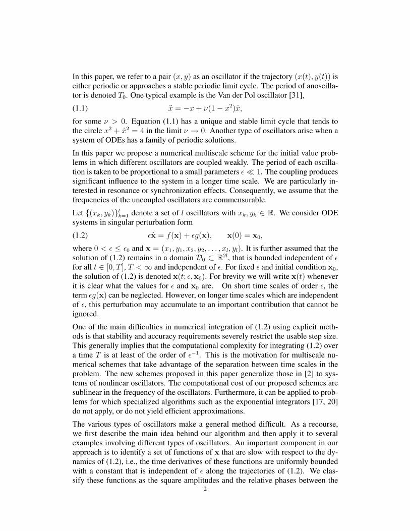
The algorithm described in Section 2.2 was implemented using the slow chart ξwith ε = 10−4 and ω = 10. Other parameters are H = 0.5, h = ε/15, η = 25ε and(2.6) as a kernel. Both micro and Macro solvers employ a fourth order Runge-Kuttascheme. We compare results for A = 0 and A = 10. Figure 4.1 depicts the timeevolution of the amplitude of the Van der Pol oscillator, I1 = x2

1 + y21 . In order

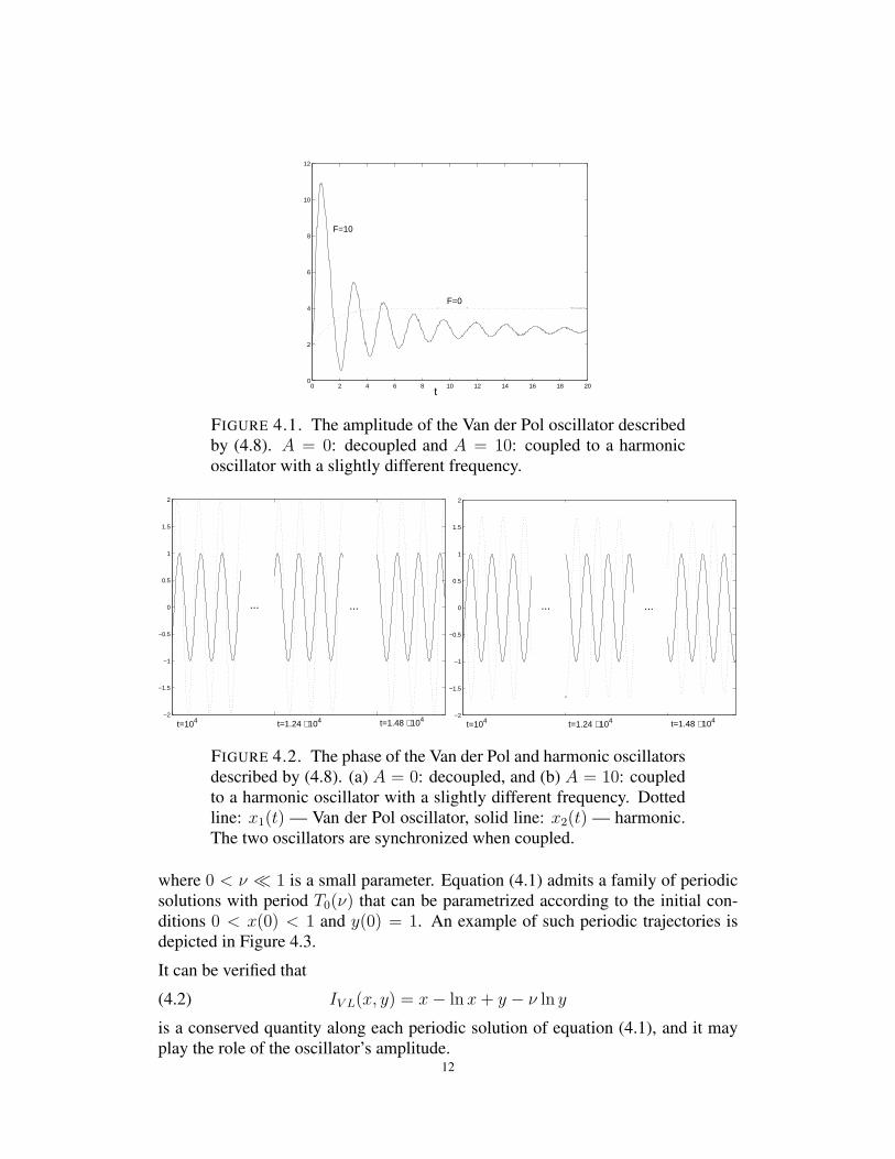
to observe the effect of the relative phase, we plot in Figure 4.2 the values of x1

and x2 during three different runs of the micro-solver. In Figure 4.2a, A = 0 andthe two oscillators are decoupled. We see that the two oscillators slowly drift outof phase due to the slightly different frequencies. With A = 10 the oscillators arecoupled and maintain a constant relative phase. The phenomenon of phase locking,(also called entrainment or synchronization) is well known for nonlinear oscillators[16, 28].

4.2. The Volterra-Lotka oscillator. In this section we consider the Volterra-Lotkaoscillator, which is treated as a benchmark case for oscillators that admit a con-served quantity. The Volterra-Lotka oscillator is given by the ODE

(4.1)

{x = x(1− ν−1y)

y = ν−1y(x− 1),11

0 2 4 6 8 10 12 14 16 18 200

2

4

6

8

10

12

t

F=10

F=0

FIGURE 4.1. The amplitude of the Van der Pol oscillator describedby (4.8). A = 0: decoupled and A = 10: coupled to a harmonicoscillator with a slightly different frequency.

−2

−1.5

−1

−0.5

0

0.5

1

1.5

2

... ...

t=104 t=1.24 ⋅ 104 t=1.48 ⋅ 104 −2

−1.5

−1

−0.5

0

0.5

1

1.5

2

... ...

t=104 t=1.24 ⋅ 104 t=1.48 ⋅ 104

FIGURE 4.2. The phase of the Van der Pol and harmonic oscillatorsdescribed by (4.8). (a) A = 0: decoupled, and (b) A = 10: coupledto a harmonic oscillator with a slightly different frequency. Dottedline: x1(t) — Van der Pol oscillator, solid line: x2(t) — harmonic.The two oscillators are synchronized when coupled.

where 0 < ν � 1 is a small parameter. Equation (4.1) admits a family of periodicsolutions with period T0(ν) that can be parametrized according to the initial con-ditions 0 < x(0) < 1 and y(0) = 1. An example of such periodic trajectories isdepicted in Figure 4.3.

It can be verified that

(4.2) IV L(x, y) = x− lnx+ y − ν ln y

is a conserved quantity along each periodic solution of equation (4.1), and it mayplay the role of the oscillator’s amplitude.

12

Each periodic orbit can be divided into the union of two continuous open segmentsjoined by two points (xI , ν) and (xII , ν) where xI ,and xII are the solutions ofIV L(x, ν) = C0. We denote the first segment by ΓI which consists of a relativelyslow movement close to the x-axis. The second segment, ΓII , corresponds to thetrajectory along the upper arc depicted in Figure 4.3. In a duration proportional to ν,the solution goes through the upper arc and comes downs to the first segment. The

0 0.5 1 1.5 2 2.5 3 3.50

0.2

0.4

0.6

0.8

1

1.2

x

y

t=0

t=0.046, 3.373 t=3.284

t=3.31

FIGURE 4.3. The trajectory of the Volterra-Lotka oscillator (4.1)with ν = 0.01, x(0) = 0.5 and y(0) = 1.

trajectory goes from one segment to the other whenever its y component equals ν,at which location, x = 0. Away from y = ν, x > 0 when the trajectory is on ΓI andx < 0 on ΓII . This suggests that an inverse function mapping from the trajectory tosome reference time coordinate can be defined separately on each segment:

τI(x(t), y(t)) = t, for (x(t), y(t)) ∈ ΓI

andτII(x(t), y(t)) = t+ CII , for (x(t), y(t)) ∈ ΓII .

Hence, for (x, y) ∈ΓI ,

∂τI(x, y)

∂xx+

∂τI(x, y)

∂yy =

1

ε.

Away from the turning points at y = ν, the gradient for τ2(x, y) are exactly the sameas that of τ1(x, y). Denoting 1Γ as the indicator function of the set Γ we formallydefine τ and ∇τ by

τ = 1ΓI (x, y)τI(x, y) + 1ΓII (x, y)τII(x, y),

and∇τ = 1ΓI (x, y)∇τI(x, y) + 1ΓII (x, y)∇τII(x, y).

Hence,∇τ is given by (??) and (??).13

Let (X1(t), Y1(t)) denote a periodic solution of (4.1) and (X2(t), Y2(t)) denote anunperturbed harmonic oscillator with frequency ω. Similar to the approach de-scribed in Section 4.1, we define

(4.3) θ(X1, Y1, X2, Y2) = τ(X1, Y1)− ω−1 arctan(Y2

X2

).

From the discussion of Section 3.2, the slow observable ϑ defined by

d

dtϑ = ∇θ ·

X1

Y1

X2

Y2

is a well-defined continuous function of time, which is related to the relative phasebetween the oscillators.

Now, consider the weak coupling of a Volterra-Lotka and a harmonic oscillator:

(4.4)

εx1 = x1(1− ν−1y1) + εg1(x),

εy1 = ν−1y1(x1 − 1) + εh1(x),

εx2 = ωy2 + εg2(x),

εy2 = −ωx2 + εh2(x).

Thus, as we argued in Section 3.1, along each non-equilibrium trajectory of (4.4),denoted by γ(t) for convenience, we can define the relative phase between the twooscillators as a slowly changing observable satisfying

d

dtϑ =

(∇θ · (ε−1f)

)|γ(t), ϑ(0) = 0,

where f denotes the right hand side of (4.4).

As an example, the HMM algorithm was applied to (4.4) with ε = 10−5, ν = 0.2,g1 = y2

2 , h1 = 0, g2 = 0 and h2 = x1. The frequency of the harmonic oscillator istaken to be close to that of the Volterra-Lotka one, ω = 3.77/2π. The singularityat y1 = ν is not problematic since ∇θ · x is integrable. Hence, we apply a cutoffaround |y1−ν| < 10−4, which introduces an additional error evaluated by changingthe cutoff value. Improved accuracy can be obtained by using methods such asPadé approximations in order to integrate over the problematic region. Additionalparameters are H = 0.25, η = 40 (which is about 11 periods) and the integrationkernel is (2.6). The micro-solver is a fourth order Runge-Kutta scheme with stepsize h = 0.03ε. The Macro-solver is the midpoint rule. In addition, as explained inSection 3.2, we made sure that the macro-step is not taken with y1 values close toν. Figure 4.4 compares the solution of the amplitudes I1(x1, y1) = IV L(x1, y1) andI2 = x2

2 + y22 obtained by the HMM algorithm (plus signs) with that of the fourth

order Runge-Kutta method (solid line) with the same step size h = 0.03ε.14

0 1 2 3 4

1

1.4

1.8

2.2

I1

I2

FIGURE 4.4. The amplitude of the Volterra-Lotka oscillator, I1 =IV L = x1 − lnx1 + y1 − ν ln y1, and the harmonic oscillator, I2 =x2

2 + y22 . Fourth order Runge-Kutta (solid line) compared to HMM

(plus signs).

4.3. Relaxation oscillators. Consider the following ODE suggested by Dahlquistet. al. [8]

(4.1)

{x = −1− x+ 8y3

y = ν−1(−x+ y − y3),

where ν � 1 is a small parameter. The dynamics of (4.1) has a limit cycle thatis defined by the cubic polynomial x = y − y3 and the turning points dx/dy = 0on it. The limit cycle consists of four parts, ΓI,, ΓII , ΓIII , and ΓIV . ΓI and ΓIIIdenote, respectively, the upper and lower branches of this cubic polynomial whichare stable up to the turning points at which dx/dy = 0. For any initial condition, thesolution of (4.1) is attracted to one of the stable branches on anO(ν) time scale. Thetime derivative x stays positive when the trajectory is close to ΓI and negative whenclose to ΓIII . Thus, trajectories of (4.1) move close to a branch until it becomesunstable. At this point the solution is quickly attracted to the other stable branch.During the transient states, the trajectories stay close to ΓII and ΓIV . The trajectoryof the oscillator near the limit cycle is depicted in Figure 4.5. Van der Pol dubbedthe name relaxation oscillators due to the fast relaxation process at the instabilities.We shall use the structure of this limit cycle to parametrize time.

The amplitude of the relaxation oscillator can be defined by some notion of distancebetween the trajectory and the limit cycle, for example, as the difference in the ycoordinates of the trajectory and the limit cycle at some fixed x. This is effectivelya particular realization of the Poincaré map with a transversal segment x = const.Under the dynamics of (4.1), this distance converges to zero exponentially fast ina time scale of order ν.Hence, the amplitude of the oscillator can be considered adissipative variable.

15

Next, we discuss how to define the phase of the oscillator. In order to do so, weneed to make our description of the limit cycle more precise. As we alluded above,it consist of four parts: The vertical segments, ΓII and ΓIV , are defined by theintersections of x = ±2

√3/9 and x = y − y3:

ΓII = {(x, y) : x =2√

3

9, y ∈ I2},

ΓIV = {(x, y) : x = −2√

3

9, y ∈ I4},

where I2 = (b2, 2√

3/9) and I4 = (−2√

3/9, b4) are the intervals bounded by thetwo solutions of y − y3 = 2

√3/9 and y − y3 = −2

√3/9, respectively. Hence,

ΓI = {(x, y) : x = y − y3,1√3< y < b4},

ΓIII = {(x, y) : x = y − y3, b2 < y < − 1√3}.

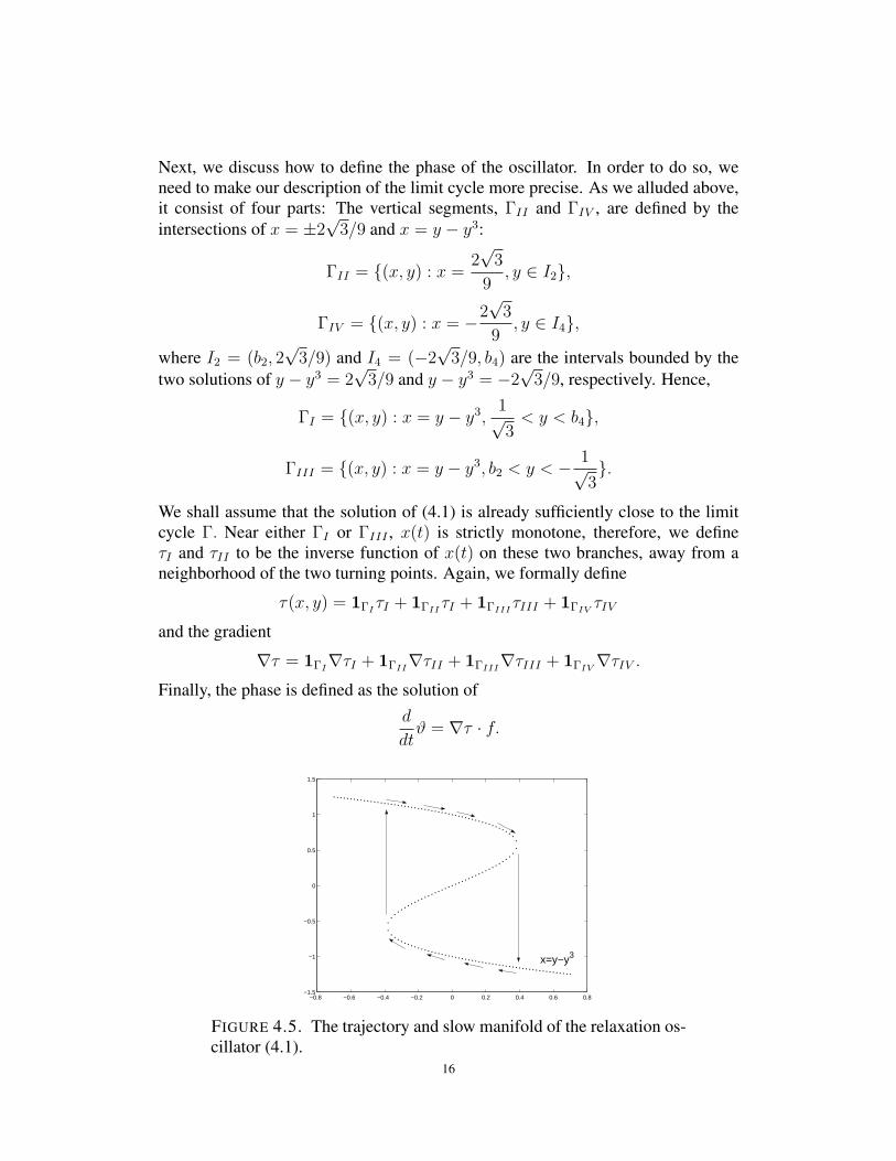
We shall assume that the solution of (4.1) is already sufficiently close to the limitcycle Γ. Near either ΓI or ΓIII , x(t) is strictly monotone, therefore, we defineτI and τII to be the inverse function of x(t) on these two branches, away from aneighborhood of the two turning points. Again, we formally define

τ(x, y) = 1ΓIτI + 1ΓIIτI + 1ΓIIIτIII + 1ΓIV τIV

and the gradient

∇τ = 1ΓI∇τI + 1ΓII∇τII + 1ΓIII∇τIII + 1ΓIV∇τIV .Finally, the phase is defined as the solution of

d

dtϑ = ∇τ · f.

−0.8 −0.6 −0.4 −0.2 0 0.2 0.4 0.6 0.8−1.5

−1

−0.5

0

0.5

1

1.5

x=y−y3

FIGURE 4.5. The trajectory and slow manifold of the relaxation os-cillator (4.1).

16

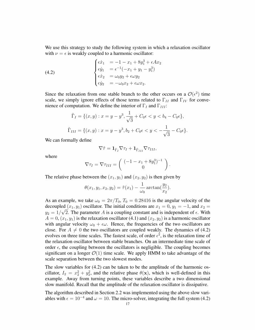
We use this strategy to study the following system in which a relaxation oscillatorwith ν = ε is weakly coupled to a harmonic oscillator:

(4.2)

εx1 = −1− x1 + 8y3

1 + εAx2

εy1 = ε−1(−x1 + y1 − y31)

εx2 = ω0y2 + εωy2

εy2 = −ω0x2 + εωx2.

Since the relaxation from one stable branch to the other occurs on a O(ε2) timescale, we simply ignore effects of those terms related to ΓII and ΓIV for conve-nience of computation. We define the interior of ΓI and ΓIII :

ΓI = {(x, y) : x = y − y3,1√3

+ C0ε < y < b4 − C0ε},

ΓIII = {(x, y) : x = y − y3, b2 + C0ε < y < − 1√3− C0ε}.

We can formally define

∇τ = 1ΓI∇τI + 1ΓIII

∇τIII ,where

∇τI = ∇τIII =

((−1− x1 + 8y3

1)−1

0

).

The relative phase between the (x1, y1) and (x2, y2) is then given by

θ(x1, y1, x2, y2) = τ(x1)− 1

ω0

arctan(y2

x2

).

As an example, we take ω0 = 2π/T0, T0 = 0.28416 is the angular velocity of thedecoupled (x1, y1) oscillator. The initial conditions are x1 = 0, y1 = −1, and x2 =y2 = 1/

√2. The parameter A is a coupling constant and is independent of ε. With

A = 0, (x1, y1) is the relaxation oscillator (4.1) and (x2, y2) is a harmonic oscillatorwith angular velocity ω0 + εω. Hence, the frequencies of the two oscillators areclose. For A 6= 0 the two oscillators are coupled weakly. The dynamics of (4.2)evolves on three time scales. The fastest scale, of order ε2, is the relaxation time ofthe relaxation oscillator between stable branches. On an intermediate time scale oforder ε, the coupling between the oscillators is negligible. The coupling becomessignificant on a longer O(1) time scale. We apply HMM to take advantage of thescale separation between the two slowest modes.

The slow variables for (4.2) can be taken to be the amplitude of the harmonic os-cillator, I2 = x2

2 + y22 , and the relative phase θ(x), which is well-defined in this

example. Away from turning points, these variables describe a two dimensionalslow manifold. Recall that the amplitude of the relaxation oscillator is dissipative.

The algorithm described in Section 2.2 was implemented using the above slow vari-ables with ε = 10−4 and ω = 10. The micro-solver, integrating the full system (4.2)

17

micro−solverh

η η

Macro−solver

x

ξH

FIGURE 4.6. An asymmetric HMM for problems involving transients.

was implemented using a forth order Runge-Kutta scheme with variable step sizein order to speed up integration along the stable branches of the limiting cycle.Hence, our scheme operates on three time scales: ε2, ε and 1. The Macro-solveruses a forward Euler scheme plus projection of the (x2, y2) oscillator onto the unitcircle. Additional parameters are H = 0.25 and η = 25ε. Due to the dissipativenature of the fast oscillations, the micro-solver only integrates the system forwardin time and the resulting algorithmic structure is shown in Figure 4.6. Finally, it isimportant that macroscopic steps are not taken too close to the boundary of a chart,particularly if the boundary corresponds to a turning point of the trajectory. Thiscan be avoided by running the micro-solver to time η + T0, and then choosing asub-segment of length η with a convenient mid-point for taking the macro-step.

We compare results for A = 0 and A = 40. Figure 4.2 depicts the values of x1 andx2 during three different runs of the micro-solver. In Figure 4.7a, A = 0 and theoscillators are decoupled. We see that the two oscillators slowly drift out of phasedue to the slight difference in oscillator frequencies. With A = 40 the oscillatorsare coupled and maintain a constant relative phase. Figure 4.8 depicts the solutionof (4.2) with ω0 = 4π/T0, i.e, the frequency of the harmonic oscillator is slightlydifferent than twice the frequency of the relaxation oscillator. With A = 40 therelaxation oscillator is synchronized with exactly half the frequency of the harmonicone. This phenomenon is referred to 1-2 entrainment or resonance.

5. CONCLUSION

Previously in [2], we have proposed an approach for decomposing a vector fieldinto its fast and slow constituents using the concept of slow variables. The de-composition is used in an algorithm that efficiently integrates the slow parts of thedynamics without fully resolving the fast parts globally in time. In this paper we

18

−1

−0.8

−0.6

−0.4

−0.2

0

0.2

0.4

0.6

0.8

1

... ...

t=1 ⋅ 104 t=5 ⋅ 104 t=9 ⋅ 104 −1

−0.8

−0.6

−0.4

−0.2

0

0.2

0.4

0.6

0.8

1

... ...

t=1 ⋅ 104 t=5 ⋅ 104 t=9 ⋅ 104

FIGURE 4.7. The phase of the relaxation and harmonic oscillatorsdescribed by (4.2). (a) A = 0: decoupled, and (b) A = 40: coupledto a harmonic oscillator with a slightly different frequency. Dottedline: x2(t) — harmonic oscillator, solid line: x1(t) — relaxation.The two oscillators are synchronized when coupled.

−1

−0.8

−0.6

−0.4

−0.2

0

0.2

0.4

0.6

0.8

1

... ...

t=1 ⋅ 104 t=5 ⋅ 104 t=9 ⋅ 104

FIGURE 4.8. Example of 1-2 entrainment between a relaxation os-cillator and a harmonic one. Dotted line: x2(t) — harmonic oscilla-tor, solid line: x1(t) — relaxation.

further develop this idea and extend it to fully nonlinear oscillators. This includesoscillators which are very different in nature from harmonic oscillators. The slowvariables are classified as amplitudes and relative phases, in analogy to correspond-ing variables for harmonic oscillators. The notion of relative phase is defined byconstructing inverse functions that maps the periodic orbits to time. Following theHMM framework, the time evolution of the slow variables in the coupled system iscomputed using only the fly short-time simulations of the full system. Thus, we areable to compute efficiently the slow behavior of the system using large time steps.

19

ACKNOWLEDGMENTS

Support from NSF through Grant DMS-0714612 is gratefully acknowledged. Wethank Nick Tanushev and Eric Vanden-Eijnden for useful suggestions, correctionsand discussions. Tsai’s research is partially supported by an Alfred P. Sloan Fellow-ship. Tsai and Engquist thank the Isaac Newton Institute for Mathematical Sciencesfor hosting parts of this research. Tsai also thanks the National Center for Theoret-ical Sciences at Taipei.

REFERENCES

[1] A. Abdulle. Fourth order Chebyshev methods with recurrence relation. SIAM J. Sci. Comput.,23(6):2041–2054 (electronic), 2002.

[2] G. Ariel, B. Engquist, and R. Tsai. A multiscale method for highly oscillatory ordinary dif-ferential equations with resonance. Math. Comp., 2008. Accepted. A preprint is available as aUCLA CAM report.

[3] D. Cohen, T. Jahnke, K. Lorenz, and C. Lubich. Numerical integrators for highly oscillatoryhamiltonian systems: A review. In Analysis, Modeling and Simulation of Multiscale Problems,pages 553–576. Springer Berlin Heidelberg, 2006.

[4] G. Dahlquist. Convergence and stability in the numerical integration of ordinary differentialequations. Mathematica Scandinavica, 4:33–53, 1956.

[5] G. Dahlquist. Stability and error bounds in the numerical integration of ordinary differentialequations. Kungl. Tekn. Högsk. Handl. Stockholm. No., 130:87, 1959.

[6] G. Dahlquist. A special stability problem for linear multistep methods. Nordisk Tidskr.Informations-Behandling, 3:27–43, 1963.

[7] G. Dahlquist. Error analysis for a class of methods for stiff non-linear initial value problems.In Numerical analysis (Proc. 6th Biennial Dundee Conf., Univ. Dundee, Dundee, 1975), pages60–72. Lecture Notes in Math., Vol. 506. Springer, Berlin, 1976.

[8] G. Dahlquist, L. Edsberg, G. Skollermo, and G. Soderlind. Are the numerical methods andsoftware satisfactory for chemical kinetics? In Numerical Integration of Differential Equationsand Large Linear Systems, volume 968 of Lecture Notes in Math., pages 149–164. Springer-Verlag, 1982.

[9] W. E. Analysis of the heterogeneous multiscale method for ordinary differential equations.Commun. Math. Sci., 1(3):423–436, 2003.

[10] W. E and B. Engquist. The heterogeneous multiscale methods. Commun. Math. Sci., 1(1):87–132, 2003.

[11] B. Engquist and Y.-H. Tsai. Heterogeneous multiscale methods for stiff ordinary differentialequations. Math. Comp., 74(252):1707–1742, 2003.

[12] W. Gautschi. Numerical integration of ordinary differential equations based on trigonometricpolynomials. Numerische Mathematik, 3:381–397, 1961.

[13] C. W. Gear and I. G. Kevrekidis. Projective methods for stiff differential equations: problemswith gaps in their eigenvalue spectrum. SIAM J. Sci. Comput., 24(4):1091–1106 (electronic),2003.

[14] C.W. Gear and K.A. Gallivan. Automatic methods for highly oscillatory ordinary differentialequations. In Numerical analysis (Dundee, 1981), volume 912 of Lecture Notes in Math., pages115–124. Springer, 1982.

[15] J. Grasman. Asymptotic methods for relaxation oscillations and applications, volume 63 ofApplied Mathematical Sciences. Springer-Verlag, 1987.

[16] J. Guckenheimer and P. Holmes. Nonliner oscillations, dynamical systems and bifurcations ofvector fields, volume 42 of Applied Mathematical Sciences. Springer-Verlag, 1990.

20

[17] E. Hairer, C. Lubich, and G. Wanner. Geometric numerical integration, volume 31 of SpringerSeries in Computational Mathematics. Springer-Verlag, Berlin, 2002. Structure-preserving al-gorithms for ordinary differential equations.

[18] E. Hairer and G. Wanner. Solving ordinary differential equations. II, volume 14 of SpringerSeries in Computational Mathematics. Springer-Verlag, 1996.

[19] M.W. Hirsch, S. Smale, and R. Devaney. Differential equations, dynamical systems, and anintroduction to chaos. Academic Press, Boston, 2004.

[20] M. Hochbruck, C. Lubich, and H. Selhofer. Exponential integrators for large systems of differ-ential equations. SIAM J. Sci. Comp., 19:1552–1574, 1998.

[21] J. Kevorkian and J. D. Cole. Multiple Scale and Singular Perturbation Methods, volume 114of Applied Mathematical Sciences. Springer-Verlag, New York, Berlin, Heidelberg, 1996.

[22] H.-O. Kreiss. Difference methods for stiff ordinary differential equations. SIAM J. Numer.Anal., 15(1):21–58, 1978.

[23] H.-O. Kreiss. Problems with different time scales. In Acta numerica, 1992, pages 101–139.Cambridge Univ. Press, 1992.

[24] V. I. Lebedev and S. A. Finogenov. The use of ordered Cebyšhev parameters in iteration meth-ods. Ž. Vycisl. Mat. i Mat. Fiz., 16(4):895–907, 1084, 1976.

[25] B. Leimkuhler and S. Reich. Simulating Hamiltonian dynamics, volume 14 of CambridgeMonographs on Applied and Computational Mathematics. Cambridge University Press, 2004.

[26] J. E. Marsden and M. West. Discrete mechanics and variational integrators. Acta Numer.,10:357–514, 2001.

[27] R.L. Petzold, O.J. Laurent, and Y. Jeng. Numerical solution of highly oscillatory ordinarydifferential equations. Acta Numerica, 6:437–483, 1997.

[28] A. Pikovsky, M. Rosenblum, and J. Kurths. Phase synchronization in regular and chaotic sys-tems. Int. J. Bifurcation and Chaos, 10(10):2291–2305, 2000.

[29] J. A. Sanders and F. Verhulst. Averaging Methods in Nonlinear Dynamical Systems, volume 59of Applied Mathematical Sciences. Springer-Verlag, New York, Berlin, Heidelberg, Tokyo,1985.

[30] R.E. Scheid. The accurate numerical solution of highly oscillatory ordinary differential equa-tions. Mathematics of Computation, 41(164):487–509, 1983.

[31] B. Van der Pol. On relaxation oscillations. Phil. Mag. 2, 2:978–992, 1926.[32] F. Verhulst. Nonlinear differential equations and dynamical systems. Springer, Berlin, New

York, 1996.

DEPARTMENT OF MATHEMATICS, THE UNIVERSITY OF TEXAS AT AUSTIN, AUSTIN, TX, 78712,USA

E-mail address: ariel@math.utexas.edu

E-mail address: engquist@math.utexas.edu

E-mail address: ytsai@math.utexas.edu

21