Int J Adv Manuf Technol (2016) 87:1797–1811DOI 10.1007/s00170-016-8571-y

ORIGINAL ARTICLE

Numerical modeling of the thermal contact in metal formingprocesses

J. M. P. Martins1 ·D. M. Neto1 · J. L. Alves2 ·M. C. Oliveira1 ·L. F. Menezes1

Received: 3 November 2015 / Accepted: 29 February 2016 / Published online: 12 March 2016© Springer-Verlag London 2016

Abstract Heat flow across the interface of solid bodies incontact is an important aspect in several engineering appli-cations. This work presents a finite element model for theanalysis of thermal contact, which takes into account theeffect of contact pressure and gap dimension in the heatflow across the interface between two bodies. Addition-ally, the frictional heat generation is also addressed, whichis dictated by the contact forces predicted by the mechan-ical problem. The frictional contact problem and thermalproblem are formulated in the frame of the finite elementmethod. A new law is proposed to define the interfacial heattransfer coefficient (IHTC) as a function of the contact pres-sure and gap distance, enabling a smooth transition betweentwo contact status (gap and contact). The staggered schemeused as coupling strategy to solve the thermomechanicalproblem is briefly presented. Four numerical examples are

D. M. Netodiogo.neto@dem.uc.pt

J. M. P. Martinsjoao.pmartins@dem.uc.pt

J. L. Alvesjlalves@dem.uminho.pt

M. C. Oliveiramarta.oliveira@dem.uc.pt

L. F. Menezesluis.menezes@dem.uc.pt

1 CEMUC, Department of Mechanical Engineering,University of Coimbra, polo II, Rua Luıs Reis Santos,Pinhal de Marrocos, 3030-788 Coimbra, Portugal

2 CMEMS, Centre for MicroElectroMechanical SystemsResearch, University of Minho, Campus de Azurm,4800-058 Guimares, Portugal

presented to validate the finite element model and high-light the importance of the proposed law on the predictedtemperature.

Keywords Thermal contact · Interfacial heat transfercoefficient (IHTC) · Frictional heat generation · Finiteelement method (FEM) · Coupling strategy · Metal forming

1 Introduction

The heat flow across the interface between two contactingbodies plays an important role in many engineering appli-cations, such as the automotive [52], microelectronics [54],metalworking [37], and gas turbine industries [17]. The heatflow across contacting interfaces is commonly quantified bythe interfacial heat transfer coefficient (IHTC), which is theinverse of the resistance to heat flow [28]. This resistanceis the cause of temperature discontinuity at the interfacebetween the bodies. Three different methods can be used tocalculate the IHTC from experimentally measured temper-atures [55], which are: the heat balance method, the Beck’smethod [9], and the finite element analysis based optimiza-tion method (FEA method). Zhao et al. [55] have comparedthese three methods using a hot stamping experimental set-up to determine the IHTC evolution during the process.They concluded that the Beck’s method presents the mostaccurate results, followed by the heat balance method andfinally, the FEA method, which has the less accurate results,due to the fact that the model used only provides a constantvalue for the IHTC evolution. IHTC evaluation studies havebeen increasing during the last few years, in several areas ofindustry. Recently, Dureja et al. [16] have proposed a newexperimental set-up, for the IHTC determination betweenpressure and calandria tubes from a heavy water reactor.

�

1798 Int J Adv Manuf Technol (2016) 87:1797–1811

They highlighted a linear increase of the IHTC with thecontact pressure up to 10 MPa. Akar et al. [3] have alsoinvestigated the IHTC evolution during the casting process,because the IHTC is an important factor for reliable resultson the numerical simulation of casting processes. The IHTCalso plays a crucial role in hot/warm sheet metal formingprocesses, since the heat exchanges on the interface of thesheet are important for the temperature control and, conse-quently, the mechanical properties of the final part [21, 29,33]. In fact, the numerical modeling of the interfacial heattransfer requires the prior determination of the IHTC [27].Thus, the accurate evaluation of this parameter is essentialfor the thermal and mechanical analysis of any system. Nev-ertheless, the modeling of the heat transfer across a contactinterface is one of the well-known problems in the numer-ical simulation of thermal boundary conditions. Typically,the IHTC is assumed constant in the numerical modeling,although it is known that it is affected by several factors,such as, the surface roughness and flatness, contact pres-sure, mechanical properties of the contacting surfaces andgap distance [26, 45]. The roughness and flatness of the con-tact surface have a significant effect on the IHTC, whichdecreases with the increase in surface flatness and decreasein roughness [11]. Indeed, the real contact area is a verysmall fraction of the nominal contact area (2 % for metal-lic contact). The real contact occurs only in certain discretepoints, at the top of asperities [28]. The contact pressure hasa close connection with the real contact area, since the defor-mation of the contacting asperities induced by the contactpressure increases the real contact area and, consequently,the IHTC value. The effects of the contact pressure duringthe hot forging process were investigated by Bai et al. [5].They reported an exponential increase of the IHTC up to100 MPa, followed by a slightly increase for higher pres-sures. Chang et al. [13] measured the IHTC during the hotstamping of an advanced high strength steel, obtaining thesame trend for the IHTC with the contact pressure, propos-ing a power law to fit the experimental data. Since thedeformation of the asperities is directly defined by the hard-ness of the contacting surfaces, it is greater for soft materialsthan for hard ones. Therefore, soft materials present a largereffective contact surface area and, consequently, higher val-ues of the IHTC than hard materials. There are a numberof empirical and semi-empirical correlations for the deter-mination of the IHTC (or contact condutance) in functionof the roughness, contact pressure, and the hardness of thematerial, for example the Yovanovich’s plastic model [53]and the Mikic’s plastic deformation model [34]. However,this models tend to overestimate the IHTC value. Xu andXu [50] pointed a possible reason for that, which is the useof a constant hardness value in the calculation. In fact, thehardness varies with the temperature, but it is difficult toevaluate this evolution [31].

The heat transfer across the contact interface occursby conduction through asperities in contact, convectionthrough the fluid inside the gap, and by radiation acrossthe gap [47]. The radiation can be negligible for tempera-tures lower than 300 ◦C [28]. The gap fluid conductance isless efficient than the conduction through asperities. Thus,the increasing of the gap separating the contact surfacesdecreases the IHTC value. In fact, Merklein et al. [32]investigated the influence of the gap distance between twocontacting surfaces on the IHTC in hot stamping, conclud-ing that the increase of the gap yields a IHTC decrease,independent of the temperature of the contacting surfaces.For the worst case reported, the IHTC value has decayedapproximately 240 W/m2 K, between a gap distance of 1 to1.5 mm, and only 40 W/m2 K, between a gap distance of 1.5to 2 mm.

The sliding contact between solids generates energy,which originates an increase of temperature at the inter-face and affects the mechanical behavior of the system. Theconversion of mechanical energy into frictional heating isusually assumed around 80–100 % [6], while the remainingenergy is dissipated in abrasive wear and changes of surfacetopography. The amount of factors involved in the frictionalheating (contacting materials, sliding velocity, normal pres-sure, roughness, temperature, etc.) increases significantlythe complexity of this phenomenon [10]. Nevertheless, anaccurate prediction of the temperature rise due to frictionalheating is crucial for thermal stress analysis and thermalwear modeling [7, 22]. Typically, the heat generated is mod-eled based on the applied load, sliding velocity, and frictioncoefficient [15]. In the numerical modeling, the frictioncoefficient is commonly assumed as constant, although itdepends on the roughness of the contacting surfaces, lubri-cation conditions, temperature of the surfaces, applied load,and plastic deformation [14, 24]. Besides this assumption,the total amount of heat generated at the interface has tobe distributed between the contacting bodies, requiring thedefinition of a coefficient of partition, which depends onseveral factors as shown in tribological studies [7, 44]. Nev-ertheless, it is usually assumed equally partitioned betweenthe two bodies.

The finite element analysis of thermomechanical prob-lems allows to understand the thermal effects occurring atthe contact interface of two bodies, which is of crucial inter-est for industrial applications [2, 38, 41, 48, 49]. Thus,the improvement of the actual algorithms is essential forthe development of the numerical simulation, namely inthe field of sheet metal forming. In fact, the concept oflightweight vehicles led to the introduction of new mate-rials, such as advanced high strength steels [23], whichcontributed for the accentuated role of frictional heatingin conventional cold sheet metal forming [42] and theneed to develop temperature supported sheet metal forming

Int J Adv Manuf Technol (2016) 87:1797–1811 1799

processes, such as hot and warm sheet metal forming [20,25, 46]. Hence, this work presents an algorithm able tomodel the conductive heat flow across the contact interfacebetween a deformable body and a rigid obstacle. The pro-posed model takes into account both the contact pressureand the gap distance in the evaluation of the IHTC. Besides,the heat generation at the interface due to frictional contactis also predicted by the model.

The outline of the paper is the following. Section 2 is ded-icated to the formulation of contact and heat transfer prob-lems and to the description of the global thermomechanicalcoupled algorithm, with emphasis on the thermal problem.In Section 3, four numerical examples are used to validatethe proposed model, which highlights the importance of anaccurate modeling of the heat exchanges on the interface.

2 Finite element formulation

2.1 Frictional contact

This section contains the formulation of the frictional con-tact problem between a deformable body involving largedeformation and a rigid obstacle with arbitrary shape, asshown in Fig. 1. The domain occupied by the deformablebody B in the current configuration is represented by theopen set �. The closure of the open set denotes the boundarysurface γ , which is divided into three disjoint open sets: γ =γu∪γσ ∪γc representing the Dirichlet, Neumann, and contactportions, respectively. The body is subject to prescribeddisplacements u on the Dirichlet region of the boundary γu,prescribed tractions t on the Neumann region of the boundaryγσ and to contact constraints on the remaining region γc.

Assuming quasi-static response (no inertia terms), theboundary value problem formulated in the current config-uration is governed by the following balance equations:

⎧⎨

⎩

∇ · σ + b = 0 in �,

t = t at γσ ,

u = u at γu,

(1)

z

x

y

Obstacle

mn

u

c

σ

t u

Fig. 1 Deformable body in contact with a rigid obstacle and respectiveboundary conditions

where σ is the Cauchy stress tensor and b denotes the bodyforces applied in the body volume. In order to include con-straints resulting from the frictional contact between thedeformable body and the rigid obstacle, the kinematic andstatic contact variables are defined. The contact interac-tion between the deformable body and the rigid obstacleis expressed by the gap function and the tangential rel-ative sliding. The normal gap is evaluated in each slavenode, where the counterpart point on the master surfaceis evaluated by means of the projection of the slave nodeon the master surface. Considering a slave node xs of thedeformable body, the normal gap function is defined as:

gn(xs) = (xs − xm) · nm, (2)

where xm indicates the closest point from the slave onto themaster surface and nm is the outer normal vector to the mas-ter surface at the projection point (Fig. 1). This definition ofthe normal gap function establishes that the function valueis positive when the contact is open; otherwise, it will benegative. The tangential sliding of the deformable body overthe rigid surface, which is necessary for modeling frictioneffects, is evaluated through the change of the closest pointprojection. The tangential slip increment of a slave node onthe rigid surface is defined in the incremental form as:

gt = �ξατm

α , α = 1, 2, (3)

where τmα are the covariant tangential basis vectors of

the master surface and �ξα

denotes the increment of theconvective coordinates.

The static variable used to model the frictional contactinteractions is the contact traction vector in the current con-figuration, which is resolved into its normal and tangentialcomponents:

t = pnnm + tt (4)

where pn is normal contact pressure and tt denotes thefriction traction. This Cauchy stress vector represents phys-ically the force exerted by the slave node on the mastersurface. The constraints related with impenetrability andfriction conditions are expressed considering relationshipsbetween the previously presented kinematic and static vari-ables. The contact traction in the normal and in the tan-gential directions are coupled with the normal gap and thetangential slip increment, respectively. The unilateral con-tact condition, which defines the physical requirements ofimpenetrability and compressive interaction between thebodies, is given by:

gn ≥ 0, pn ≤ 0, pngn = 0 (5)

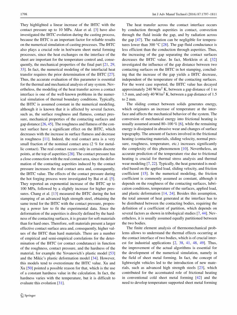
which must hold for all slave nodes. The relationshipbetween the normal gap and the normal contact pressure ispresented in Fig. 2a. The frictional response is formulated

1800 Int J Adv Manuf Technol (2016) 87:1797–1811

gap

contact

np

ng

tt

slip

stick

np

tg

(b)(a)

Fig. 2 Relationship between the normal gap and the normal contactpressure (a) and relationship between the friction force value and theslip increment (b)

using the Coulombs friction law, establishing that the fric-tion force depends on the contact pressure. The constraintsimposed by the friction law are described by the followingthree conditions:

‖tt‖ − μ|pn| ≤ 0,

‖tt‖ − μ|pn| gt‖gt‖ = 0,

‖gt‖(‖tt‖ − μ|pn|) = 0, (6)

where μ is the friction coefficient. If the value of the frictionforce has not reached the Coulomb’s threshold, the node isnot allowed to move in the tangential direction (stick sta-tus). On the other hand, when the friction force reaches theCoulomb’s limit, the node moves in the tangential direction(slip status). Figure 2b shows the relationship between thefriction force value and the slip increment.

2.2 Heat transfer

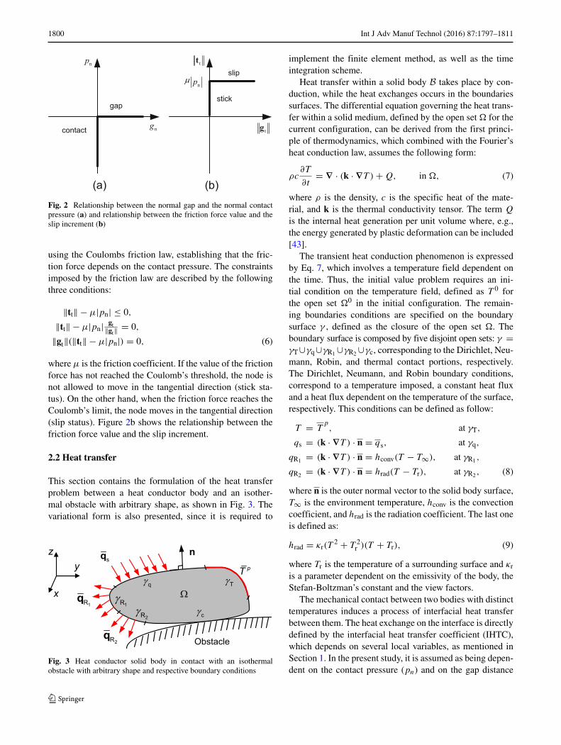
This section contains the formulation of the heat transferproblem between a heat conductor body and an isother-mal obstacle with arbitrary shape, as shown in Fig. 3. Thevariational form is also presented, since it is required to

Obstacle

n

T

c

q

sqpT

1R

2Rq

z

x

y

2R

1Rq

Fig. 3 Heat conductor solid body in contact with an isothermalobstacle with arbitrary shape and respective boundary conditions

implement the finite element method, as well as the timeintegration scheme.

Heat transfer within a solid body B takes place by con-duction, while the heat exchanges occurs in the boundariessurfaces. The differential equation governing the heat trans-fer within a solid medium, defined by the open set � for thecurrent configuration, can be derived from the first princi-ple of thermodynamics, which combined with the Fourier’sheat conduction law, assumes the following form:

ρc∂T

∂t= ∇ · (k · ∇T ) + Q, in �, (7)

where ρ is the density, c is the specific heat of the mate-rial, and k is the thermal conductivity tensor. The term Qis the internal heat generation per unit volume where, e.g.,the energy generated by plastic deformation can be included[43].

The transient heat conduction phenomenon is expressedby Eq. 7, which involves a temperature field dependent onthe time. Thus, the initial value problem requires an ini-tial condition on the temperature field, defined as T 0 forthe open set �0 in the initial configuration. The remain-ing boundaries conditions are specified on the boundarysurface γ , defined as the closure of the open set �. Theboundary surface is composed by five disjoint open sets: γ =γT∪γq ∪γR1 ∪γR2 ∪γc, corresponding to the Dirichlet, Neu-mann, Robin, and thermal contact portions, respectively.The Dirichlet, Neumann, and Robin boundary conditions,correspond to a temperature imposed, a constant heat fluxand a heat flux dependent on the temperature of the surface,respectively. This conditions can be defined as follow:

T = Tp, at γT,

qs = (k · ∇T ) · n = qs, at γq,

qR1 = (k · ∇T ) · n = hconv(T − T∞), at γR1 ,

qR2 = (k · ∇T ) · n = hrad(T − Tr), at γR2 , (8)

where n is the outer normal vector to the solid body surface,T∞ is the environment temperature, hconv is the convectioncoefficient, and hrad is the radiation coefficient. The last oneis defined as:

hrad = κr(T2 + T 2

r )(T + Tr), (9)

where Tr is the temperature of a surrounding surface and κr

is a parameter dependent on the emissivity of the body, theStefan-Boltzman’s constant and the view factors.

The mechanical contact between two bodies with distincttemperatures induces a process of interfacial heat transferbetween them. The heat exchange on the interface is directlydefined by the interfacial heat transfer coefficient (IHTC),which depends on several local variables, as mentioned inSection 1. In the present study, it is assumed as being depen-dent on the contact pressure (pn) and on the gap distance

Int J Adv Manuf Technol (2016) 87:1797–1811 1801

(gn), allowing to predict accurately a wide range of contactconditions involved in forming processes. The heat flux onthe contact surface γc is given by:

qint = hint(pn, gn)(T − Tobs), at γc (10)

where hint is the IHTC and T and Tobs are the surface tem-

peratures of the solid body and the isothermal obstacle. TheIHTC is modeled with an empirical law, which takes intoaccount the dependence on the contact pressure and on thegap distance, the mathematical function proposed is inspiredin the experimental results of the macro-contact analysis [5,13, 32], and is expressed by:

hint(pn, gn) ={hmed + (

hsup − hmed)(1 − exp (m1 pn)) if pn < 0 ∧ gn = 0

hinf − (hinf − hmed) exp (−m2gn) if gn ≥ 0 ∧ pn = 0(11)

where hsup and hinf are the upper and lower threshold val-ues for the IHTC. The piecewise definition of the IHTCallows accounting both mechanical contact status (gap andcontact). The graphical representation of this function isdepicted in Fig. 4, presenting two horizontal asymptotes,corresponding to hsup and hinf. When the contact pressuretends to infinity (negative), the IHTC is equal to hsup, i.e.,the upper threshold value. On the other hand, when the gapdistance tends to infinity (positive), the IHTC is equal tohinf, corresponding to the lower threshold value, i.e. the nat-ural convection coefficient value. The parameters hmed, m1

and m2 allows to control the rate of the increase/decrease ofthe IHTC. This empirical law is attractive from the numer-ical point of view because it promotes a smooth transitionof the IHTC between the two contact status (gap and con-tact), while allowing an accurate fitting to the IHTC valuesdetermined from experimental temperatures.

The frictional heat generation should be taken intoaccount when the friction is considered in the mechanicalcontact. Considering the frictional contact problem involv-ing a solid body and an isothermal obstacle, the heat flux due tofrictional heat generation at the interface can be expressed as:

qfrict = β(ξ tt · gt

), at γc (12)

where ξ represents the fraction of generated energy con-verted into heat, which is partitioned between the solid body

int suph h

inth

int medh h

ng

np

int infh h

Fig. 4 Interfacial heat transfer coefficient

and the isothermal obstacle. Therefore, the parameter β

defines the total amount of heat dissipated to the solid body.The frictional heat is directly proportional to the frictionforce tt and the increment of tangential slip velocity gt, ashighlighted in Eq. 12.

Applying the principle of virtual temperature [8] and pro-ceeding to the decomposition of the domain, the boundaryvalue problem defined in Eq. 7 can be given in the matrixform as:

CT + KT = f (13)

where the matrixes and vector are given by:

C =∫

�

ρcNTNTd� (14)

K =∫

�

MTkMTd� +∫

γtc

hintNTs NsTdγ (15)

f =∫

γtc

hintTobsNTs dγ +

∫

γtc

qfrictdγ (16)

where N and Ns are the vectors of the shape functions asso-ciated to the volume and surface of the body and M = ∇N.The transient heat conduction Eq. 13 is integrated over thetime using the generalized trapezoidal method [18], whichis a one time step method, given by:

Tt+�t = Tt + [αTt+�t + (1 − α) Tt

]�t (17)

where t is the time instant and �t the time increment.The parameter α can vary between 0 and 1. Dependingon the value attributed to this parameter, the generalizedtrapezoidal method takes the form of different integrationmethods, namely Euler forward method (α = 0), Crank-Nickolson method (α = 1/2), Galerkin method (α = 2/3),and Euler backward method (α = 1) [18].

2.3 Staggered coupling scheme

The numerical solution of the thermal problem arising in theinterface between two bodies requires the resolution of themechanical problem in order to evaluate the contact forcesand relative distances. Thus, the algorithm adopted to per-form the thermomechanical coupling is briefly presented.

1802 Int J Adv Manuf Technol (2016) 87:1797–1811

The problem is separated into one mechanical problemwhere the contact forces are evaluate and one thermal prob-lem for the temperature evaluation. The separately treatmentof each of these subproblems is completely implicit andis performed recurring to the Newton-Raphson iterativemethod, to ensure that the thermal and mechanical fieldsare consistent at the end of each time step. Two types ofschemes can be used to perform the coupling between thetwo problems: (i) a fully coupled scheme, where the twoproblems are treated simultaneously; (ii) a staggered cou-pled scheme, where the two problems are treated separately[12]. The former scheme has a better computational effi-ciency, particularly when the thermal problem is linear [19].The staggered scheme is adopted in the present study, wherethe mechanical problem is solved for a previously calculatedtemperature field, while the thermal problem is solved in thecurrent equilibrium configuration [1, 49].

This algorithm was implemented in DD3IMP in-housefinite element code, which has been developed to simulatesheet metal forming processes [30, 40]. The deformationof the body is described by an update Lagrangian formula-tion, where the region occupied by the deformable body ata given instant t is denoted by configuration C [t]. The con-tact constrains are enforced using an augmented Lagrangianmethod, where the Lagrangian multiplier vector (λ) repre-sents the contact force vector needed to fulfil the frictionalconstrains [4]. Thus, the nodal displacements (u) and con-tact forces (λ) are evaluated in the mechanical problem,while the temperature field (T), as the new unknown, isevaluated in the thermal problem. The mechanical problemcomprises a prediction phase, based on an explicit approach,and a correction phase, based on an implicit approach.Within the explicit approach, an approximated first solu-tion is calculated for the nodal displacements u[t+�,trial] andnodal frictional contact forces λ[t+�,trial], for the incrementt + �t . Then, an rmin strategy is employed to restrict theincrement size, in order to improve the convergence rate ofthe mechanical correction phase, which is based on a fullyimplicit algorithm of Newton-Raphson type to solve, withina single iterative loop, the non-linearities related with boththe mechanical behavior of material and the contact withfriction [36, 39, 51]. The resolution of the thermal problemis carried out after achieving the mechanical equilibrium.The solution of the thermal problem uses the updated con-figuration C [t+�t], u[t+�t], λ[t+�t] and the temperaturefield of the last instant T[t]. In this phase, the Eq. 13 mustbe solved, using one of the different methods, depending onthe value assumed for the previously mentioned parameterα, in Eq. 17. The result is a new thermal field T[t+�t]. Themain steps of the global thermomechanical algorithm aresummarized in Table 1.

3 Numerical examples

In this section, four examples of frictionless and frictionalthermal contact are presented. In order to demonstrate theaccuracy of the algorithm and to highlight the influenceof the IHTC on the predicted temperature, the first threeexamples are dedicated to a specific problem. They canbe divided as frictional heat generation, influence of gapdistance on heat flow, and influence of the contact pres-sure on the heat flow. The last example comprises all theseproblems. In all examples, the mechanical behavior of thedeformable bodies is assumed perfectly elastic, in order tofocus the analysis at the interface behavior. For the samereason, the heat exchanges for the environment, by convec-tion and radiation, are neglected. Besides, all the examplesuse solid linear finite elements (8-node hexahedral), for theresolution of both problems, thermal and mechanical. Theobstacles or tools are considered as rigid bodies, and theirouter surfaces are modeled with Nagata patches [35, 36].The parameter α in Eq. 17 is always set to a value of (α =1), which corresponds to an Euler backward time integrationscheme.

3.1 Frictional heating of a block

The first example involves the frictional sliding of an elas-tic block over a fixed rigid surface and it was adaptedfrom Wriggers and Miehe [48]. This example allows topredict the temperature rise due to the frictional heat gen-eration, neglecting the heat lost to the rigid surface bycontact. Thus, the only heat fluxes that are considered on theboundary surface are only due to frictional heat generation.The temperature evolution is evaluated for the deformablebody (block), while the temperature of the rigid surface

Table 1 Global thermomechanical algorithm

1: Process input data.

2: Initialize variables for the current configuration C [t].3: Increment time step by �t .

4: Mechanical problem: Prediction phase.

4.1: Determine u[t+�,trial] and λ[t+�,trial].4.2: Correct the increment size �t , with the rmin strategy.

4.3: Update the current configuration, C [t+�t,trial].5: Mechanical problem: Correction phase.

5.1: Determine u[t+�t] and λ[t+�t].5.2: Update the current configuration, C [t+�t].

6: Thermal problem.

6.1: Determine T[t+�t].7: Go to point 2 and repeat the process until the total time is attained.

Int J Adv Manuf Technol (2016) 87:1797–1811 1803

210 N/mmp

Node A

Node B

0.2

1.25 mm 3.75 mm

1.25 mm

x

z

Fig. 5 Geometry setting of the frictional heating of a block problem and discretization

is assumed constant. The initial configuration of the prob-lem and the finite element mesh adopted for the deformablebody are presented in Fig. 5, assuming plane strain condi-tions. First, a pressure of p = 10 N/mm2 is applied on the topof the block, followed by a prescribed horizontal displace-ment of 3.75 mm within 3.75 × 10−3 s, from the left to theright. The displacement is discretized into 100 time steps,as in the original example [48]. The friction is modeled bythe Coulomb’s law, with a friction coefficient of μ = 0.2.It is assumed that the energy dissipated by friction is totallyconverted into heat and the total amount of heat is equallypartitioned between the body and the rigid surface. Thus,the parameters ξ and β on the Eq. 12 assume the value of1 and 0.5, respectively. The material properties are listed inTable 2 as well as the initial temperature condition.

The applied pressure and displacement of the block leadsto the presence of a relative tangential contact force, whichcauses the heat generation. The nodal contact forces in theblock, evaluated by the mechanical problem, are presentedin Fig. 6, for two instants. Before imposing the horizon-tal displacement, the contact force vectors are symmetric(Fig. 6a), while during the sliding the maximum values offriction force are localized on the front nodes (Fig. 6b), lead-ing to higher temperature due to the frictional sliding. The

Table 2 Material properties and initial conditions

Young’s modulus E 70,006 N/mm2

Poisson’s ratio ν 0.3

Density ρ 2.7×10−9 Ns2/mm4

Expansion coefficient α 23.8×10−6 ◦C−1

Conductivity k 150 Ns/◦C

Capacity c 0.9×109 mm2/s2 ◦C

Reference temperature Tre f 0 ◦C

Initial temperature Tini 0 ◦C

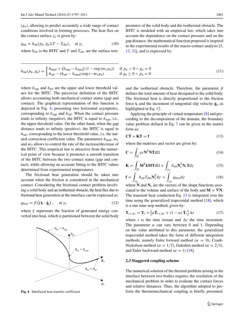
temperature distribution in the block is presented in Fig. 7,for three different instants during the sliding, namely dis-placements u = 1.275, 2.55, and 3.75 mm. The maximumvalue of temperature is reached in node A (Fig. 5), despite

1.25

1.15

1.06

0.96

0.86

0.77

[N]

1.69

2.12

1.27

0.85

0.42

0.00

[N]

(a)

(b)Fig. 6 Distribution of the contact forces: a instant immediately beforethe displacement imposition and b during the sliding for the timeinstant of t = 2.55×10−3 s

1804 Int J Adv Manuf Technol (2016) 87:1797–1811

Fig. 7 Temperature distributionfor the displacements: u = 1.25,2.5, and 3.75 mm 1.275 mmu

2.55 mmu

3.75 mmu

31.275x10 st

32.55x10 st

33.75x10 st

[º ]T C

the maximum tangential force not being located on this node(Fig. 6b), as a result of the heat conduction phenomenon.

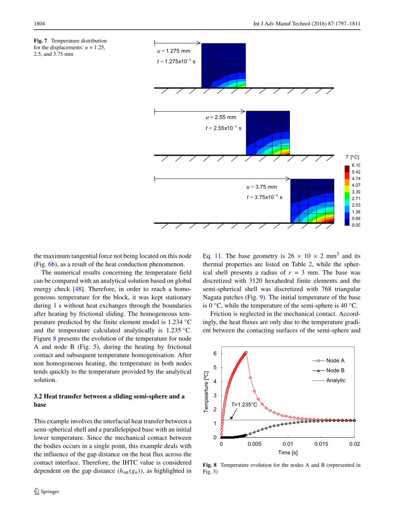
The numerical results concerning the temperature fieldcan be compared with an analytical solution based on globalenergy check [48]. Therefore, in order to reach a homo-geneous temperature for the block, it was kept stationaryduring 1 s without heat exchanges through the boundariesafter heating by frictional sliding. The homogeneous tem-perature predicted by the finite element model is 1.234 ◦Cand the temperature calculated analytically is 1.235 ◦C.Figure 8 presents the evolution of the temperature for nodeA and node B (Fig. 5), during the heating by frictionalcontact and subsequent temperature homogenisation. Afternon homogeneous heating, the temperature in both nodestends quickly to the temperature provided by the analyticalsolution.

3.2 Heat transfer between a sliding semi-sphere and abase

This example involves the interfacial heat transfer between asemi-spherical shell and a parallelepiped base with an initiallower temperature. Since the mechanical contact betweenthe bodies occurs in a single point, this example deals withthe influence of the gap distance on the heat flux across thecontact interface. Therefore, the IHTC value is considereddependent on the gap distance (hint(gn)), as highlighted in

Eq. 11. The base geometry is 26 × 10 × 2 mm3 and itsthermal properties are listed on Table 2, while the spher-ical shell presents a radius of r = 3 mm. The base wasdiscretized with 3120 hexahedral finite elements and thesemi-spherical shell was discretized with 768 triangularNagata patches (Fig. 9). The initial temperature of the baseis 0 ◦C, while the temperature of the semi-sphere is 40 ◦C.

Friction is neglected in the mechanical contact. Accord-ingly, the heat fluxes are only due to the temperature gradi-ent between the contacting surfaces of the semi-sphere and

0

1

2

3

4

5

6

0 0.005 0.01 0.015 0.02

Tem

pear

ture

[ºC

]

Time [s]

Node A

Node B

Analytic

T=1.235°C

Fig. 8 Temperature evolution for the nodes A and B (represented inFig. 5)

Int J Adv Manuf Technol (2016) 87:1797–1811 1805

zy

x

Fig. 9 Geometrical setting for problem 2 and respective finite elementmesh

the parallelepiped base. The semi-sphere centre is initiallylocated at 4 mm from the left hand of the base and is moved18 mm in the x-direction, within 18 s using a incrementaldisplacement of �u = 0.5 mm. Four cases are compared,one with a constant value of IHTC and three with the IHTCdependent on the gap distance between the bodies, given byEq. 11 using different values for the m2. For the case ofthe constant IHTC, a value of 2500×10−3 N/(smm◦C) wasselected. The three sets of parameters selected for the vari-able IHTC definition are presented in Table 3. The evolutionof the IHTC value with the gap distance is presented inFig. 10, for the three sets of parameters presented in Table 3,as well as for the constant IHTC.

The maximum value of gap distance for which the inter-facial heat transfer occurs was restricted to 2 mm in thepresent example. The pattern of gap distance distribution,which defines the area where the heat flux occurs, is con-stant during the motion, due to the insignificant deformationof the base. Figure 11 presents the gap distance for eachslave node of the base with projection, for the instant corre-sponding to a displacement of the semi-sphere of u = 9 mmand a time instant of t = 9 s.

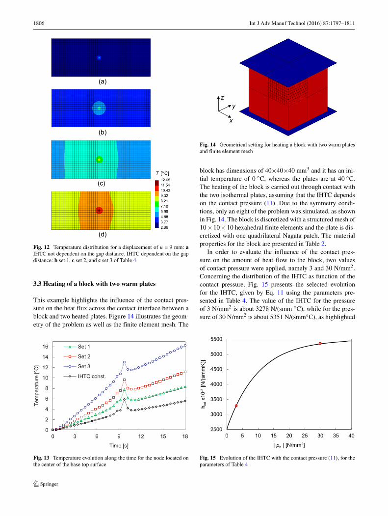
The temperature distribution on the base is presentedin Fig. 12 for a displacement of the semi-sphere of u =9 mm, considering the four cases of the IHTC. The temper-ature distribution presented in Fig. 12a considers a constant

Table 3 Set of parameter for example 2

Set 1 hinf 0 N/(smm◦C)

hmed 2500×10−3 N/(smm◦C)

m2 8

Set 2 hinf 0 N/(smm◦C)

hmed 2500×10−3 N/(smm◦C)

m2 4

Set 3 hinf 0 N/(smm◦C)

hmed 2500×10−3 N/(smm◦C)

m2 2

0

500

1000

1500

2000

2500

0.0 0.5 1.0 1.5 2.0

h int

x10-3

[N/(s

.mm

.K)]

gn [mm]

Constant IHTC

Set 1

Set 2

Set 3

Fig. 10 Evolution of the IHTC with the gap distance (11), for theparameter sets presented in Table 3 and for the constant value of 2500×10−3 N/(smm◦C)

value for the IHTC, while the interfacial heat transfer occursonly with physical contact. On the other hand, the temper-ature distribution considering an IHTC dependent on thegap distance is presented in Fig. 12b–d for the parametersets 1, 2, and 3 listed in Table 3, respectively. The increaseof temperature is lower using the constant value of IHTC(Fig. 12a), because the heat flux occurs only in a single con-tact point. On the other hand, assuming an IHTC dependenton the gap distance leads to higher temperatures, as shownin Fig. 12b–d, for lower m2 values. In fact, the thermalenergy transferred for the base is higher, since the con-ditions to define the area where heat transference occurswas amplified (Fig. 10). Figure 13 presents the tempera-ture evolution for a node located in the middle of the topsurface of the base. The trend for the temperature evolu-tion is identical with a constant or variable IHTC, showingthe influence of the zero gap instant. Moreover, the influ-ence of the IHTC value is highlighted in the temperatureincrease, which is higher for the IHTC dependent of the gapdistance due to the increase of the area where the heat fluxarises.

n [mm]g

Fig. 11 Normal gap distance for the nodes with projection, for adisplacement of u = 9 mm

1806 Int J Adv Manuf Technol (2016) 87:1797–1811

[º ]T C

(c)

(a)

(b)

(d)

Fig. 12 Temperature distribution for a displacement of u = 9 mm: aIHTC not dependent on the gap distance. IHTC dependent on the gapdistance: b set 1, c set 2, and c set 3 of Table 4

3.3 Heating of a block with two warm plates

This example highlights the influence of the contact pres-sure on the heat flux across the contact interface between ablock and two heated plates. Figure 14 illustrates the geom-etry of the problem as well as the finite element mesh. The

0

2

4

6

8

10

12

14

16

0 3 6 9 12 15 18

Tem

pera

ture

[ºC

]

Time [s]

Set 1

Set 2

Set 3

IHTC const.

Fig. 13 Temperature evolution along the time for the node located onthe center of the base top surface

zy

x

Fig. 14 Geometrical setting for heating a block with two warm platesand finite element mesh

block has dimensions of 40×40×40 mm3 and it has an ini-tial temperature of 0 ◦C, whereas the plates are at 40 ◦C.The heating of the block is carried out through contact withthe two isothermal plates, assuming that the IHTC dependson the contact pressure (11). Due to the symmetry condi-tions, only an eight of the problem was simulated, as shownin Fig. 14. The block is discretized with a structured mesh of10 × 10 × 10 hexahedral finite elements and the plate is dis-cretized with one quadrilateral Nagata patch. The materialproperties for the block are presented in Table 2.

In order to evaluate the influence of the contact pres-sure on the amount of heat flow to the block, two valuesof contact pressure were applied, namely 3 and 30 N/mm2.Concerning the distribution of the IHTC as function of thecontact pressure, Fig. 15 presents the selected evolutionfor the IHTC, given by Eq. 11 using the parameters pre-sented in Table 4. The value of the IHTC for the pressureof 3 N/mm2 is about 3278 N/(smm ◦C), while for the pres-sure of 30 N/mm2 is about 5351 N/(smm◦C), as highlighted

2500

3000

3500

4000

4500

5000

5500

0 5 10 15 20 25 30 35 40

h int

x10-3

[N/(s

mm

K)]

| pn | [N/mm2]

Fig. 15 Evolution of the IHTC with the contact pressure (11), for theparameters of Table 4

Int J Adv Manuf Technol (2016) 87:1797–1811 1807

Table 4 Set of parameters for example 3

hsup 5500 ×10−3 N/(smm◦C)

hmed 2500 ×10−3 N/(smm◦C)

m1 0.1

in Fig. 15 (red dots). The total heating time is 60 s and theincrement of time selected was �t = 1.2 s.

Figure 16a, b presents the temperature distribution in thefirst time increment, corresponding to 1.2 s, for the pressureof 3 and 30 N/mm2, respectively. The influence of the con-tact pressure on the temperature distribution is highlighted,namely in the maximum value attained, which arises in thecontact interface. Therefore, the proposed model for theIHTC value, as function of the contact pressure, is able topredict different temperature distributions according to thecontact conditions.

Figure 17 presents the evolution of the temperature fortwo nodes, one located in the top surface of the block (node1) and the other situated 10 mm below the top surface (node2). The positions of these nodes are presented in Fig. 16. The

(a)

(b)

[ºC]T

[ºC]T

Node 2

Node 1

Node 1

Node 2

Fig. 16 Temperature distribution for the instant of 1.2 s: a pressure of3 N/mm2 and b pressure of 30 N/mm2

0

10

20

30

40

0 10 20 30 40 50 60

Tem

pera

ture

[°C

]

Time [s]

Node 1 (P=30MPa)

Node 2 (P=30MPa)

Node 1 (P=3MPa)

Node 2 (P=3MPa)

Fig. 17 Temperature evolution for two nodes. Node 1 situated on thetop surface of the block and node 2 situated 5 mm below the top surface

red lines correspond to a pressure of 3 N/mm2 and the blacklines correspond to a pressure of 30 N/mm2. The slop ofthe curves decreases with the temperature increase, becausethe thermal gradient in the contact interface is decreasing.Besides, for large values of heating time, the temperaturedifference between the selected nodes decreases, due to theheat conduction effect.

3.4 Ironing with a heated cylindrical die

This last example was designed to comprise the threeaspects focused in the last three examples, the frictionalheat generation and the influence of the gap distance andthe contact pressure on the IHTC value. The problem com-prises a rigid cylindrical shell sliding over a deformableparallelepiped base. Figure 18 illustrates the geometricalsetting and the finite element mesh of the bodies. The par-allelepiped base has dimensions of 34 × 5 × 10 mm3, while

zy

x

Fig. 18 Geometrial setting for ironing a deformable parallelepipedbase and finite element mesh

1808 Int J Adv Manuf Technol (2016) 87:1797–1811

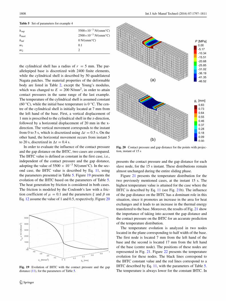
Table 5 Set of parameters for example 4

hsup 5500×10−3 N/(smm◦C)

hmed 2500×10−3 N/(smm◦C)

hinf 0 N/(smm◦C)

m1 0.1

m2 2

the cylindrical shell has a radius of r = 5 mm. The par-allelepiped base is discretized with 2400 finite elements,while the cylindrical shell is described by 50 quadrilateralNagata patches. The material properties of the deformablebody are listed in Table 2, except the Young’s modulus,which was changed to E = 200 N/mm2, in order to attaincontact pressures in the same range of the last example.The temperature of the cylindrical shell is assumed constant(60 ◦C), while the initial base temperature is 0 ◦C. The cen-tre of the cylindrical shell is initially located at 7 mm fromthe left hand of the base. First, a vertical displacement of1 mm is prescribed to the cylindrical shell in the z-direction,followed by a horizontal displacement of 20 mm in the x-direction. The vertical movement corresponds to the instantfrom 0 to 5 s, which is discretized using �t = 0.5 s. On theother hand, the horizontal movement occurs from instant 5to 20 s, discretized in �t = 0.4 s.

In order to evaluate the influence of the contact pressureand the gap distance on the IHTC, two cases are compared.The IHTC value is defined as constant in the first case, i.e.,independent of the contact pressure and the gap distance,adopting the value of 5500 × 10−3 N/(smm◦C). In the sec-ond case, the IHTC value is described by Eq. 11, usingthe parameters presented in Table 5. Figure 19 presents theevolution of the IHTC based on the parameters of Table 5.The heat generation by friction is considered in both cases.The friction is modeled by the Coulomb’s law with a fric-tion coefficient of μ = 0.1 and the parameters ξ and β onEq. 12 assume the value of 1 and 0.5, respectively. Figure 20

Fig. 19 Evolution of IHTC with the contact pressure and the gapdistance (11), for the parameters of Table 5.

(b)

n [mm]g

[MPa]P

(a)

Fig. 20 Contact pressure and gap distance for the points with projec-tion, instant of 15 s

presents the contact pressure and the gap distance for eachslave node, for the 15 s instant. These distributions remainalmost unchanged during the entire sliding phase.

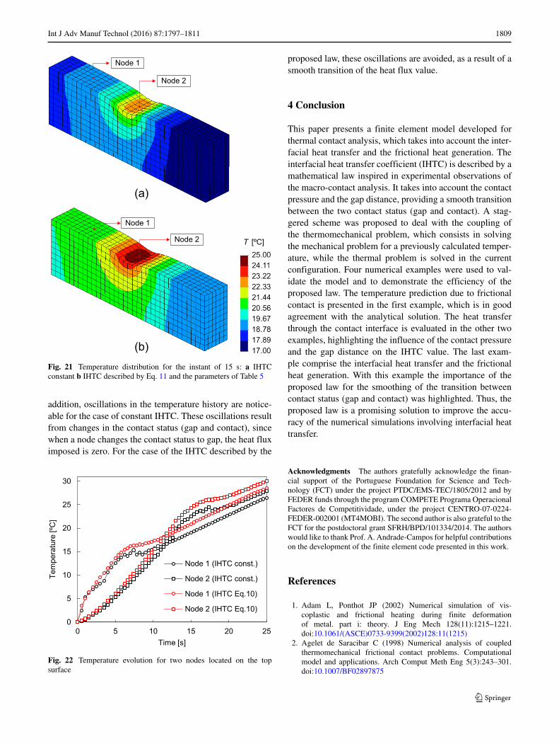
Figure 21 presents the temperature distribution for thetwo previously mentioned cases, at the instant 15 s. Thehighest temperature value is attained for the case where theIHTC is described by Eq. 11 (see Fig. 21b). The influenceof the gap distance on the IHTC has a dominant role in thissituation, since it promotes an increase in the area for heatexchanges and it leads to an increase in the thermal energytransferred to the base. Moreover, the results of Fig. 21 showthe importance of taking into account the gap distance andthe contact pressure on the IHTC for an accurate predictionof the temperature distribution.

The temperature evolution is analyzed in two nodeslocated in the plane corresponding to half width of the base.The first node is located 7 mm from the left hand of thebase and the second is located 17 mm from the left handof the base (centre node). The positions of these nodes arerepresented in Fig. 21. Figure 22 presents the temperatureevolution for these nodes. The black lines correspond tothe IHTC constant value and the red lines correspond to aIHTC described by Eq. 11, with the parameters of Table 5.The temperature is always lower for the constant IHTC. In

Int J Adv Manuf Technol (2016) 87:1797–1811 1809

[ºC]T

(b)

(a)

Node 1

Node 1

Node 2

Node 2

Fig. 21 Temperature distribution for the instant of 15 s: a IHTCconstant b IHTC described by Eq. 11 and the parameters of Table 5

addition, oscillations in the temperature history are notice-able for the case of constant IHTC. These oscillations resultfrom changes in the contact status (gap and contact), sincewhen a node changes the contact status to gap, the heat fluximposed is zero. For the case of the IHTC described by the

0

5

10

15

20

25

30

0 5 10 15 20 25

Tem

pera

ture

[ºC

]

Time [s]

Node 1 (IHTC const.)

Node 2 (IHTC const.)

Node 1 (IHTC Eq.10)

Node 2 (IHTC Eq.10)

Fig. 22 Temperature evolution for two nodes located on the topsurface

proposed law, these oscillations are avoided, as a result of asmooth transition of the heat flux value.

4 Conclusion

This paper presents a finite element model developed forthermal contact analysis, which takes into account the inter-facial heat transfer and the frictional heat generation. Theinterfacial heat transfer coefficient (IHTC) is described by amathematical law inspired in experimental observations ofthe macro-contact analysis. It takes into account the contactpressure and the gap distance, providing a smooth transitionbetween the two contact status (gap and contact). A stag-gered scheme was proposed to deal with the coupling ofthe thermomechanical problem, which consists in solvingthe mechanical problem for a previously calculated temper-ature, while the thermal problem is solved in the currentconfiguration. Four numerical examples were used to val-idate the model and to demonstrate the efficiency of theproposed law. The temperature prediction due to frictionalcontact is presented in the first example, which is in goodagreement with the analytical solution. The heat transferthrough the contact interface is evaluated in the other twoexamples, highlighting the influence of the contact pressureand the gap distance on the IHTC value. The last exam-ple comprise the interfacial heat transfer and the frictionalheat generation. With this example the importance of theproposed law for the smoothing of the transition betweencontact status (gap and contact) was highlighted. Thus, theproposed law is a promising solution to improve the accu-racy of the numerical simulations involving interfacial heattransfer.

Acknowledgments The authors gratefully acknowledge the finan-cial support of the Portuguese Foundation for Science and Tech-nology (FCT) under the project PTDC/EMS-TEC/1805/2012 and byFEDER funds through the program COMPETE Programa OperacionalFactores de Competitividade, under the project CENTRO-07-0224-FEDER-002001 (MT4MOBI). The second author is also grateful to theFCT for the postdoctoral grant SFRH/BPD/101334/2014. The authorswould like to thank Prof. A. Andrade-Campos for helpful contributionson the development of the finite element code presented in this work.

References

1. Adam L, Ponthot JP (2002) Numerical simulation of vis-coplastic and frictional heating during finite deformationof metal. part i: theory. J Eng Mech 128(11):1215–1221.doi:10.1061/(ASCE)0733-9399(2002)128:11(1215)

2. Agelet de Saracibar C (1998) Numerical analysis of coupledthermomechanical frictional contact problems. Computationalmodel and applications. Arch Comput Meth Eng 5(3):243–301.doi:10.1007/BF02897875

1810 Int J Adv Manuf Technol (2016) 87:1797–1811

3. Akar N, Azahin HM, Yalin N, Kocatepe K (2008) Experimentalstudy on the effect of liquid metal superheat and casting height oninterfacial heat transfer coefficient. Exp Heat Transfer 21(1):83–98. doi:10.1080/08916150701647785

4. Alart P, Curnier A (1991) A mixed formulation for fric-tional contact problems prone to newton like solutionmethods. Comput Methods Appl Mech Eng 92(3):353–375.doi:10.1016/0045-7825(91)90022-X

5. Bai Q, Lin J, Zhan L, Dean T, Balint D, Zhang Z (2012) An effi-cient closed-form method for determining interfacial heat transfercoefficient in metal forming. Int J Mach Tools Manuf 56:102–110.doi:10.1016/j.ijmachtools.2011.12.005

6. Banjac M, Vencl A, Otovic S (2014) Friction and wearprocesses–thermodynamic approach. Tribology in Industry 36(4)

7. Bansal DG, Streator JL (2009) A method for obtaining the tem-perature distribution at the interface of sliding bodies. Wear266(7-8):721–732. doi:10.1016/j.wear.2008.08.019

8. Bathe KJ (1996) Finite element procedures. Prentice-Hall, Engle-wood Cliffs

9. Beck JV (1970) Nonlinear estimation applied to the nonlin-ear inverse heat conduction problem. Int J Heat Mass Transfer13(4):703–716. doi:10.1016/0017-9310(70)90044-X

10. Bhushan B (2000) Modern tribology handbook, Two Volume Set.Crc Press

11. Caron EJ, Daun KJ, Wells MA (2014) Experimental heat trans-fer coefficient measurements during hot forming die quenchingof boron steel at high temperatures. Int J Heat Mass Transfer71:396–404. doi:10.1016/j.ijheatmasstransfer.2013.12.039

12. Cervera M, Codina R, Galindo M (1996) On the computa-tional efficiency and implementation of block-iterative algo-rithms for nonlinear coupled problems. Eng Comput 13(6):4–30.doi:10.1108/02644409610128382

13. Chang Y, Tang X, Zhao K, Hu P, Wu Y (2014) Investi-gation of the factors influencing the interfacial heat trans-fer coefficient in hot stamping. J Mater Process Technol.doi:10.1016/j.jmatprotec.2014.10.008

14. Chen Q, Li D (2005) A computational study of frictional heatingand energy conversion during sliding processes. Wear 259(7-12):1382–1391. doi:10.1016/j.wear.2004.12.025. 15th Interna-tional Conference on Wear of Materials

15. Conte M, Pinedo B, Igartua A (2014) Frictional heating calcu-lation based on tailored experimental measurements. Tribol Int74:1–6. doi:10.1016/j.triboint.2014.01.020

16. Dureja A, Pawaskar D, Seshu P, Sinha S, Sinha R (2015)Experimental determination of thermal contact conductancebetween pressure and calandria tubes of Indian pres-surised heavy water reactors. Nucl Eng Des 284:60–66.doi:10.1016/j.nucengdes.2014.11.025

17. Golosnoy IO, Cipitria A, Clyne TW (2009) Heat transferthrough plasma-sprayed thermal barrier coatings in gas turbines:a review of recent work. J Therm Spray Tech 18(5-6):809–821.doi:10.1007/s11666-009-9337-y

18. Hughes TJ (2012) The finite element method: linear static anddynamic finite element analysis. Courier Corporation

19. Ireman P, Klarbring A, Stromberg N (2002) Finite element algo-rithms for thermoelastic wear problems. Eur J Mech A Solids21(3):423–440. doi:10.1016/S0997-7538(02)01208-1

20. Karbasian H, Tekkaya A (2010) A review on hotstamping. J Mater Process Technol 210(15):2103–2118.doi:10.1016/j.jmatprotec.2010.07.019

21. Kaya S (2015) Nonisothermal warm deep drawing of ss304: femodeling and experiments using servo press. Int J Adv ManufTechnol:1–10. doi:10.1007/s00170-015-7620-2

22. Kennedy FE, Lu Y, Baker I (2015) Contact temperatures andtheir influence on wear during pin-on-disk tribotesting. Tribol Int82:534–542. doi:10.1016/j.triboint.2013.10.022

23. Kleiner M, Geiger M, Klaus A (2003) Manufacturing oflightweight components by metal forming. CIRP Ann ManufTechnol 52(2):521–542. doi:10.1016/S0007-8506(07)60202-9

24. Klocke F, Trauth D, Shirobokov A, Mattfeld P (2015) Fe-analysisand in situ visualization of pressure-, slip-rate-, and temperature-dependent coefficients of friction for advanced sheet metal form-ing: development of a novel coupled user subroutine for shelland continuum discretization. Int J Adv Manuf Technol:1–14.doi:10.1007/s00170-015-7184-1

25. Laurent H, Cor J, Manach P, Oliveira M, Menezes L(2015) Experimental and numerical studies on the warmdeep drawing of an al-mg alloy. Int J Mech Sci 93:59–72.doi:10.1016/j.ijmecsci.2015.01.009

26. Lee SL, Ou CR (2001) Gap formation and interfacial heat transferbetween thermoelastic bodies in imperfect contact. J Heat Transf123(2):205. doi:10.1115/1.1338133

27. Liu X, Ji K, El Fakir O, Liu J, Zhang Q, Wang L (2015) Deter-mination of the interfacial heat transfer coefficient in the hotstamping of AA7075. In: MATEC Web of conferences, EDPsciences, vol 21, p 5003

28. Madhusudana CV (1996) Thermal contact conductance. Springer29. Martins JMP, Alves JL, Neto DM, Oliveira MC, Menezes LF

(2016) Numerical analysis of different heating systems for warmsheet metal forming. Int J Adv Manuf Technol 83(5):897–909.doi:10.1007/s00170-015-7618-9

30. Menezes LF, Teodosiu C (2000) Three-dimensional numer-ical simulation of the deep-drawing process using solidfinite elements. J Mater Process Technol 97(1–3):100–106.doi:10.1016/S0924-0136(99)00345-3

31. Merchant H, Murty G, Bahadur S, Dwivedi L, Mehrotra Y(1973) Hardness-temperature relationships in metals. J Mater Sci8(3):437–442. doi:10.1007/BF00550166

32. Merklein M, Lechler J, Stoehr T (2009) Investigations onthe thermal behavior of ultra high strength boron manganesesteels within hot stamping. Int J Mater Form 2(1):259–262.doi:10.1007/s12289-009-0505-x

33. Merklein M, Wieland M, Lechner M, Bruschi S, GhiottiA (2015) Hot stamping of boron steel sheets withtailored properties: a review. J Mater Process Technol.doi:10.1016/j.jmatprotec.2015.09.023

34. Miki B (1974) Thermal contact conductance; theoreticalconsiderations. Int J Heat Mass Transfer 17(2):205–214.doi:10.1016/0017-9310(74)90082-9

35. Neto DM, Oliveira MC, Menezes LF, Alves JL (2013)Nagata patch interpolation using surface normal vectors eval-uated from the IGES file. Finite Elem Anal Des 72:35–46.doi:10.1016/j.finel.2013.03.004

36. Neto DM, Oliveira MC, Menezes LF, Alves JL (2014) ApplyingNagata patches to smooth discretized surfaces used in 3d frictionalcontact problems. Comput Methods Appl Mech Eng 271:296–320. doi:10.1016/j.cma.2013.12.008

37. Norouzifard V, Hamedi M (2014) A three-dimensional heat con-duction inverse procedure to investigate tool-chip thermal inter-action in machining process. Int J Adv Manuf Technol 74(9-12):1637–1648. doi:10.1007/s00170-014-6119-6

38. Oancea VG, Laursen TA (1997) A finite element formulation ofthermomechanical rate-dependent frictional sliding. Int J NumerMethods Eng 40(23):4275–4311. doi:10.1002/(SICI)1097-0207(19971215)40:23<4275::AID-NME257>3.0.CO;2-K

39. Oliveira MC, Menezes LF (2004) Automatic correction of the timestep in implicit simulations of the stamping process. Finite ElemAnal Des 40(13):1995–2010. doi:10.1016/j.finel.2004.01.009

Int J Adv Manuf Technol (2016) 87:1797–1811 1811

40. Oliveira MC, Alves JL, Menezes LF (2008) Algorithms and strate-gies for treatment of large deformation frictional contact in thenumerical simulation of deep drawing process. Arch ComputMeth Eng 15:113–162. doi:10.1007/s11831-008-9018-x

41. Pantuso D, Bathe KJ, Bouzinov PA (2000) A finite element proce-dure for the analysis of thermo-mechanical solids in contact. Com-put Struct 75(6):551–573. doi:10.1016/S0045-7949(99)00212-6

42. Pereira MP, Rolfe BF (2014) Temperature conditions during coldsheet metal stamping. J Mater Process Technol 214(8):1749–1758.doi:10.1016/j.jmatprotec.2014.03.020

43. Rodrigues JMC, Martins PAF (2002) Finite element modelling ofthe initial stages of a hot forging cycle. Finite Elem Anal Des38(3):295–305. doi:10.1016/S0168-874X(01)00065-8

44. Smith E, Arnell R (2014) The prediction of frictional tempera-ture increases in dry, sliding contacts between different materials.Tribol Lett 55(2):315–328. doi:10.1007/s11249-014-0359-3

45. Tariq A, Asif M (2016) Experimental investigation of thermal con-tact conductance for nominally flat metallic contact. Heat MassTransf 52(2):291–307. doi:10.1007/s00231-015-1551-1

46. Toros S, Kacar I (2008) Review of warm forming of aluminum-magnesium alloys. J Mater Process Technol 207(1-3):1–12.doi:10.1016/j.jmatprotec.2008.03.057

47. Wriggers P (2006) Computational contact mechanics, vol 30167.Springer

48. Wriggers P, Miehe C (1994) Contact constraints withincoupled thermomechanical analysis-a finite element model.Comput Methods Appl Mech Eng 113(3-4):301–319.doi:10.1016/0045-7825(94)90051-5

49. Xing H, Makinouchi A (2002) Fe modeling of thermo-elasto-plastic finite deformation and its applicationin sheet warm forming. Eng Comput 19(4):392–410.doi:10.1108/02644400210430172

50. Xu R, Xu L (2005) An experimental investigation of thermal con-tact conductance of stainless steel at low temperatures. Cryogenics45(10-11):694–704. doi:10.1016/j.cryogenics.2005.09.002

51. Yamada Y, Yoshimura N, Sakurai T (1968) Plastic stress-strainmatrix and its application for the solution of elastic-plastic prob-lems by the finite element method. Int J Mech Sci 10(5):343–354.doi:10.1016/0020-7403(68)90001-5

52. Yevtushenko A, Kuciej M, Yevtushenko O (2015) Modellingof the frictional heating in brake system with thermal resis-tance on a contact surface and convective cooling on a freesurface of a pad. Int J Heat Mass Transfer 81:915–923.doi:10.1016/j.ijheatmasstransfer.2014.11.014

53. Yovanovich M (1982) Thermal contact correlations. AIAA paper81:83–95

54. Yovanovich M (2004) Four decades of research on ther-mal contact, gap, and joint resistances in microelectron-ics - achievement award. The Ninth Intersociety Confer-ence on Thermal and Thermomechanical Phenomena InElectronic Systems (IEEE Cat No04CH37543) 2(2):182–206.doi:10.1109/ITHERM.2004.1318237

55. Zhao K, Wang B, Chang Y, Tang X, Yan J (2015) Compar-ison of the methods for calculating the interfacial heat trans-fer coefficient in hot stamping. Appl Therm Eng 79:17–26.doi:10.1016/j.applthermaleng.2015.01.018