NUMERICAL MODELING OF PLASMA CUTTING TORCHES · PDF fileNUMERICAL MODELING OF PLASMA CUTTING...
135
NUMERICAL MODELING OF PLASMA CUTTING TORCHES A THESIS SUBMITTED TO THE FACULTY OF THE GRADUATE SCHOOL OF THE UNIVERSITY OF MINNESOTA BY Madhura Shashikumar Mahajan IN PARTIAL FULFILLMENT OF THE REQUIREMENTS FOR THE DEGREE OF MASTER OF SCIENCE IN MECHANICAL ENGINEERING Adviser: Dr. Joachim V R Heberlein January 2010
Transcript of NUMERICAL MODELING OF PLASMA CUTTING TORCHES · PDF fileNUMERICAL MODELING OF PLASMA CUTTING...

NUMERICAL MODELING OF PLASMA CUTTING TORCHES
A THESIS
SUBMITTED TO THE FACULTY OF THE GRADUATE SCHOOL
OF THE UNIVERSITY OF MINNESOTA
BY
Madhura Shashikumar Mahajan
IN PARTIAL FULFILLMENT OF THE REQUIREMENTS
FOR THE DEGREE OF
MASTER OF SCIENCE IN MECHANICAL ENGINEERING
Adviser: Dr. Joachim V R Heberlein
January 2010

© Madhura Mahajan 2010

i
ACKNOWLEDGEMENTS
My sincere thanks go to Dr. Joachim V R Heberlein for his valuable supervision,
advice and guidance throughout the project. I am most grateful of Dr. Srikumar Ghorui,
Dr. He Ping Li and Dr. Juan Pablo Trelles for laying the foundation of this work for me.
I would like to thank Dr. Jon Lindsay, Dr. John Peters, Mr. Steve Liebold and Mr. Aaron
Brandt from Hypertherm Inc., the generous sponsor of the project, for their help in this
research through meaningful conversations.
I am indebted to all of my teachers at the University of Minnesota for their
thoughtful guidance throughout my coursework. I gratefully acknowledge my thesis
defense committee members Dr. John Bischof and Dr. Mahesh Krishnan for their helpful
supervision. I thank my colleagues from the HTPL group, University of Minnesota for
making the research work enjoyable. I would also like to acknowledge the help of all my
dear friends, especially Soumya for his persistent confidence in me.
Finally, I would like to express my gratitude towards my family for their
unflinching encouragement and support in various ways.

ii
DEDICATION
This thesis is dedicated to my beloved grandparents.
iii
ABSTRACT
In this thesis, a study of numerical modeling technique is performed for various
plasma cutting torches. The plasma cutting process model uses a finite volume method
based on the SIMPLEC algorithm along with the solver “FAST-2D (Flow Analysis
Simulation Tool-2D).” The source code available is a general code and does not include
any finite volume grid generator. Part of this work includes development of a generalized
finite volume grid generator dedicated for the new generation plasma torches. This
modified version of the grid generator offers users a great flexibility in grid and geometry
choice, and offers the advantage of easy variations in boundary conditions. The work
presented also includes a detailed study of the effect of the radiation model and the
cathode current density boundary condition on the distribution of the plasma field
quantities. Finally the modified version of the grid generator along with the appropriate
radiation model and current density boundary condition at the cathode are employed to
simulate selected plasma cutting torches from Hypertherm Inc.

iv
TABLE OF CONTENTS
LIST OF TABLES ....................................................................................................... vii
LIST OF FIGURES ..................................................................................................... viii
1. INTRODUCTION ....................................................................................................1
1.1 Objective ...........................................................................................................4
2. MODELING OF PLASMA CUTTING PROCESS ..................................................5
2.1 The plasma cutting process ................................................................................5
2.2 Modeling approach ............................................................................................6
2.2.1 Torch movement .................................................................................................. 7
2.2.2 Material melting................................................................................................... 8
2.2.3 Material removal .................................................................................................. 9
2.3 Plasma generation model ...................................................................................9
2.4 Governing equations ........................................................................................ 12
2.4.1 Basic assumptions .............................................................................................. 12
2.4.2 Continuity equation for species „s‟ ..................................................................... 13
2.4.3 Momentum equation .......................................................................................... 14
2.4.4 Electron energy equation .................................................................................... 15
2.4.5 Heavy-particle energy equation .......................................................................... 16
2.4.6 Electric potential equation .................................................................................. 16
2.4.7 Magnetic potential equation ............................................................................... 17
2.4.8 Terms in conservation equations ........................................................................ 17
2.5 Boundary conditions ........................................................................................ 19
2.6 Property data ................................................................................................... 21
2.7 Features of FAST-2D ...................................................................................... 22
2.8 Solution procedure .......................................................................................... 24
3. GRID GENERATION ............................................................................................ 26
3.1 Introduction ..................................................................................................... 26
3.2 Old grid generator ........................................................................................... 27
3.2.1 Control points of the plasma torch geometry ...................................................... 27
3.2.2 Coordinates extracted from the dimensions ........................................................ 28

v
3.2.3 Zones in radial direction (X-zones) .................................................................... 29
3.2.4 Zones in axial direction (Y-zones) ...................................................................... 30
3.2.5 Zone boundary functions .................................................................................... 31
3.2.6 Functions employed for generating grids of varying densities ............................. 32
3.2.7 Geometric limitations in FAST-2D and MAKEGRID......................................... 35
3.2.8 Current geometry/mesh-generation routine ......................................................... 36
3.3 New geometry/mesh-generation routine........................................................... 37
3.4 Summary of features of new mesh generation routine ...................................... 38
3.5 New X- and Y- zones ...................................................................................... 38
3.6 Sample grids generated by the grid generation subroutine: ............................... 42
4. MODELING OF RADIATION LOSSES ............................................................... 44
4.1 Introduction ..................................................................................................... 44
4.2 Energy transport in thermal plasmas ................................................................ 44
4.3 Net volumetric radiation loss ........................................................................... 46
4.4 The effective volumetric radiation loss approximation ..................................... 47
4.5 Cutting torch energy balance ........................................................................... 51
5. EFFECT OF CATHODE CURRENT DENSITY BOUNDARY CONDITION ...... 54
5.1 Introduction ..................................................................................................... 54
5.2 Initial profile used for the simulation ............................................................... 56
5.3 Effect of current density boundary condition at cathode ................................... 58
5.4 Simulation results with various current densities for Reff = 0.5 mm .................. 59
6. RESULTS AND DISCUSSION ............................................................................. 62
6.1 Simulation of HT2000 200A O2/Air cutting torch ............................................ 62
6.1.1 About the torch (www.hypertherm.com, 2009) ................................................... 62
6.1.2 Process parameters ............................................................................................. 63
6.1.3 Input velocity calculations from inlet flow rate ................................................... 65
6.1.4 Generated Grid .................................................................................................. 66
6.1.5 Initial simulation results ..................................................................................... 67
6.2 Variations in simulation ................................................................................... 74
6.2.1 Effect of radiation .............................................................................................. 74
6.2.2 Solution for off-axis velocity peaks .................................................................... 76

vi
6.2.3 Swirl velocity boundary condition correction ..................................................... 77
6.2.4 Simulation with input velocity profile ................................................................ 80
6.2.5 Te / Th ratio issue ................................................................................................ 85
6.2.6 Second order exit boundary condition ................................................................ 89
6.2.7 Issue with torch exit condition ............................................................................ 91
6.3 Simulation of HT4400 400A O2/Air torch ....................................................... 92
6.3.1 About the torch (www.hypertherm.com, 2009) ................................................... 92
6.3.2 Process parameters ............................................................................................. 95
6.3.3 Input velocity calculations from inlet flow rate ................................................... 96
6.3.4 Generated grid and simulation results: ................................................................ 97
6.4 Simulation of a 300A O2/Air torch................................................................. 101
6.4.1 Process parameters ........................................................................................... 101
6.4.2 Input velocity calculations from inlet flow rate ................................................. 102
6.4.3 Generated grid and simulation results: .............................................................. 103
7. CONCLUDING REMARKS AND RECOMMENDATIONS............................... 107
7.1 Concluding remarks....................................................................................... 107
7.2 Recommendations ......................................................................................... 109
8. BIBLIOGRAPHY ................................................................................................ 110
APPENDIX A: VARIABLES IN FAST-2D ................................................................ 113
APPENDIX B: SUBROUTINES AND OUTPUT FILES IN NEQ CODE ................... 116
APPENDIX C: SOLUTION FIELDS FOR A RANGE OF CURRENT DENSITY
PROFILE BOUNDARY CONDITIONS AT THE CATHODE FOR REFF = 0.5 MM IN
HT4400 TORCH ......................................................................................................... 117

vii
LIST OF TABLES
Table 2.1: Terms in conservation equations ................................................................... 18
Table 2.2: A typical set of boundary conditions ............................................................. 20
Table 2.3: FAST-2D at a glance ..................................................................................... 22
Table 3.1: Control points‟co-ordinates ........................................................................... 28
Table 3.2: Comparison between old and proposed geometry/mesh-generation routine ... 38
Table 4.1: Terms in the thermal energy conservation equations..................................... 45
Table 4.2: Energy balance in a plasma torch .................................................................. 52
Table 5.1: Peak temperatures with various cathode current densities and radiation models
...................................................................................................................................... 61
Table 6.1: Steady state process parameters and torch specifications (200A torch) .......... 64
Table 6.2: Steady state parameters converted to code parameters (200A torch) .............. 64
Table 6.3: Earlier and current torch exit boundary conditions......................................... 89
Table 6.4: Steady state process parameters and torch specifications (400A torch) .......... 95
Table 6.5: Steady state parameters converted to code parameters (400A torch) .............. 95
Table 6.6: Steady state process parameters and torch specifications (300A torch) ........ 101
Table 6.7: Steady state parameters converted to code parameters (300A torch) ............ 101

viii
LIST OF FIGURES
Figure 2.1: A typical plasma torch (www.hypertherm.com, 2009) ...................................5
Figure 2.2: A thermal plasma discharge (Schnick, Füssel, & Zschetzsche, 2006) ........... 10
Figure 2.3 Basics of MHD (Schnick, Füssel, & Zschetzsche, 2006) ............................... 11
Figure 2.4: Schematic diagram for HT2000 oxygen plasma cutting torch
(www.hypertherm.com, 2009) ....................................................................................... 11
Figure 2.5: Generic form of conservation equations (Ghorui, Heberlein, & Pfender, 2007)
...................................................................................................................................... 17
Figure 2.6: A typical computational domain with boundary conditions (Li, Heberlein, &
Pfender, 2004) ............................................................................................................... 19
Figure 2.7: Flow chart for NEQ code ............................................................................. 25
Figure 3.1: Control points and dimensions of plasma torch geometry in older version of
grid generator (Ghorui, Heberlein, & Pfender, 2007) ..................................................... 27
Figure 3.2: Frame for grid generation with zone boundaries (Ghorui, Heberlein, &
Pfender, 2007) ............................................................................................................... 29
Figure 3.3: Zones in radial direction (X-zones) (Ghorui, Heberlein, & Pfender, 2007) ... 30
Figure 3.4: Zones in axial direction (Y-zones) (Ghorui, Heberlein, & Pfender, 2007) .... 31
Figure 3.5: Zone boundary functions (Ghorui, Heberlein, & Pfender, 2007) .................. 31
Figure 3.6: Example of varying density grid (Ghorui, Heberlein, & Pfender, 2007) ....... 32
Figure 3.7: Varying density grid asymetric about the center (Ghorui, Heberlein, &
Pfender, 2007) ............................................................................................................... 33
Figure 3.8: Varying density grid symmetric about the center (Ghorui, Heberlein, &
Pfender, 2007) ............................................................................................................... 33
Figure 3.9: Assigning x-coordinates using the grid density functions (Ghorui, Heberlein,
& Pfender, 2007) ........................................................................................................... 34
Figure 3.10: Assigning y coordinates using the grid density functions (Ghorui, Heberlein,
& Pfender, 2007) ........................................................................................................... 34
Figure 3.11: New geometry/mesh-generation specification for the file MAKEGRID.f ... 37
Figure 3.12: Zones along the x (top) and y (bottom) coordinates used to characterize
general plasma torch geometries .................................................................................... 40
Figure 3.13: Flow chart for grid generation subroutine ................................................... 41
Figure 3.14: Grid for HT2000 (200A O2/air process) ..................................................... 42
Figure 3.15: Grid for HT4400 (400A O2/air process) ..................................................... 42
Figure 3.16: Grid for vented torch (400A O2/air process) ............................................... 43
Figure 4.1: Effective net radiative emission coefficient for oxygen as a function of
temperature: data previously used in FAST-2D (Krey & Morris, 1970), and new radiation
data by (Gleizes & Cressault, 2007) for two effective absorption radii (Reff = 0.0 & 0.5
mm) ............................................................................................................................... 49

ix
Figure 4.2: Effective net radiative emission coefficient for oxygen as a function of
temperature (T) and effective absorption radius (Reff) for 1 atm (Gleizes & Cressault,
2007) ............................................................................................................................. 50
Figure 4.3: Temperature and emission coefficient distribution in the HT4400 torch. Top
row: electron temperature distributions (left, Reff = 0 mm; right Reff = 0.5 mm). Bottom
row: net emission coefficient (left, Reff = 0 mm; right Reff = 0.5 mm) (Trelles, Heberlein,
& Pfender, 2007) ........................................................................................................... 53
Figure 5.1: Cathode current density vs. electrode temperature for various work functions
(Zhou & Heberlein, 1998).............................................................................................. 55
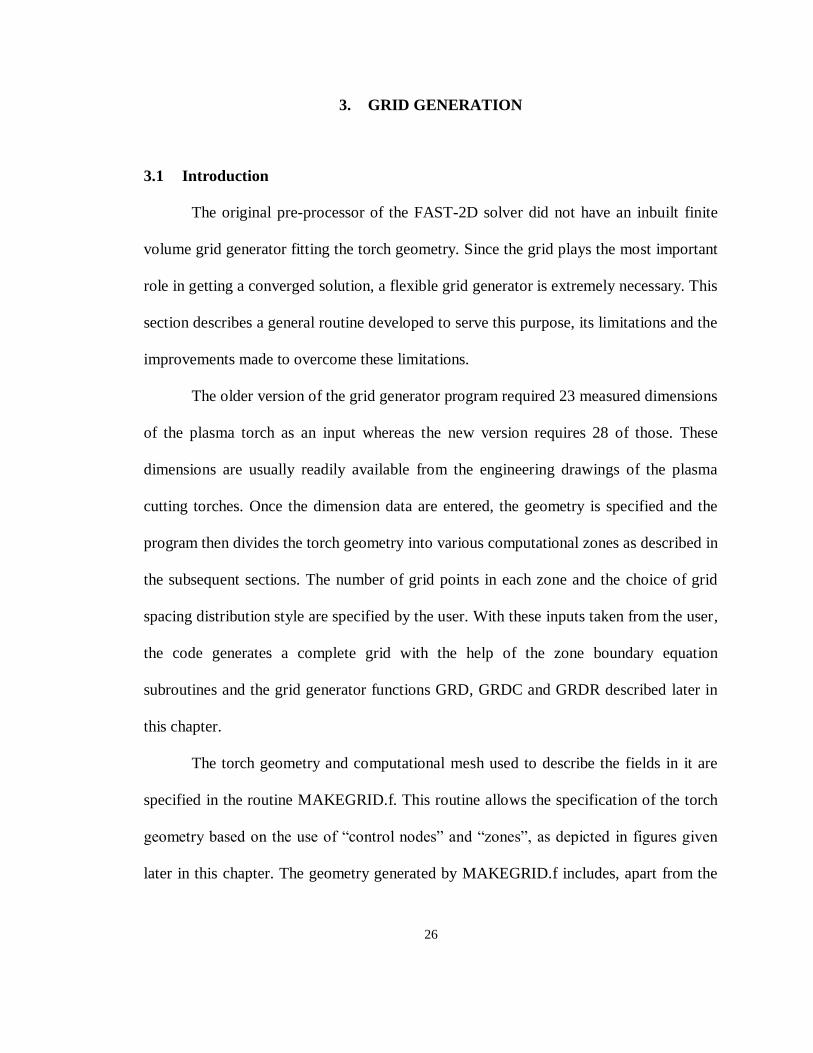
Figure 5.2: Axial current density profile with conservation of total current (Ghorui,
Heberlein, & Pfender, 2007) .......................................................................................... 57
Figure 5.3: Various axial current density profiles used as boundary condition at cathode
where c is constant in equation for profiles given by ............................... 59
Figure 5.4: Temperature profiles at the nozzle exit in HT4400 torch for the current
density profiles given in Figure 5.3 ................................................................................ 59
Figure 6.1: Schematic of HT2000 torch (dimensions in mm) (Li, Heberlein, & Pfender,
2005) ............................................................................................................................. 62
Figure 6.2: Simulation domain (dimensions in mm) (Li, Heberlein, & Pfender, 2005) ... 63
Figure 6.3: Mesh for HT2000 torch ............................................................................... 66
Figure 6.4 Command window showing convergence of FAST-2D for simulation of
HT2000 200A O2/Air cutting plasma torch .................................................................... 67
Figure 6.5: Residual plot for HT2000 torch .................................................................... 68
Figure 6.6: Results of simulation of HT2000 O2/Air 200A plasma torch (upper half)
electron temperature distribution and (lower half) heavy-particle temperature distribution
...................................................................................................................................... 69
Figure 6.7: Temperature profile at the nozzle exit in HT2000 torch................................ 70
Figure 6.8: Velocity distributions in HT2000 torch ........................................................ 71
Figure 6.9: Axial velocity profile at nozzle exit in HT2000 torch showing off-axis peaks
...................................................................................................................................... 72
Figure 6.10: Electrical characteristics of HT2000: (top) electric potential distribution and
(bottom) distribution of axial current density in the region in front of the cathode. ......... 72
Figure 6.11: Electron and heavy-particle temperature distributions in HT2000 torch: (left)
Reff = 0.5 mm (right) Reff = 0.0 mm ................................................................................. 74
Figure 6.12: Velocity plots in HT2000 torch: (left) Reff = 0.5 mm (right) Reff = 0.0 mm... 75
Figure 6.13: Radial temperature profiles at the nozzle exit in HT2000 torch .................. 75
Figure 6.14: Elimination of off-axis peaks by grid refining ............................................ 76
Figure 6.15: Swirl velocity w m/s in HT2000 torch ........................................................ 78
Figure 6.16: Incorrect w.r inlet boundary condition........................................................ 78

x
Figure 6.17: Correct w.r inlet boundary condition .......................................................... 79
Figure 6.18: Swirl velocity (w m/s) plot with corrected boundary conditions ................. 79
Figure 6.19: A sample section of torch from CFDesign simulation ................................ 81
Figure 6.20:Comparison of grids for original simulation and simulation with inlet
velocity profile .............................................................................................................. 81
Figure 6.21: Input velocity profiles for the plasma simulation ........................................ 82
Figure 6.22: Comparison of temperature plots for simulation with inlet velocity profile
and simulation with single point velocity injection ......................................................... 83
Figure 6.23: Comparison of velocity plots for simulation with inlet velocity profile and
simulation with single point velocity injection ............................................................... 83
Figure 6.24: Comparison of axial current density plots for simulation with inlet velocity
profile and simulation with single point velocity injection ............................................. 84
Figure 6.25: Comparison of electric potential plots for simulation with inlet velocity
profile and simulation with single point velocity injection ............................................. 84
Figure 6.26: Augmentation of properties beyond Te / Th = 20 and Te = 45000 (Ghorui,
Heberlein, & Pfender, 2006) .......................................................................................... 85
Figure 6.27: Plot of Te / Th for HT2000 torch ................................................................. 86
Figure 6.28: Density truncation due to excessively high Te / Th ratios ............................ 87
Figure 6.29: Corrected values of Te / Th ratios near nozzle wall ..................................... 88
Figure 6.30: Axial velocity u (m/s) along the torch centerline ........................................ 91
Figure 6.31: Cool-core electrode in HT4400 .................................................................. 92
Figure 6.32: Section of HT4400 with radial dimensions (in mm) ................................... 93
Figure 6.33: Section of HT4400 with axial dimensions (in mm)..................................... 94
Figure 6.34: Mesh for HT4400 torch.............................................................................. 97
Figure 6.35: Electron and heavy-particle temperature distributions in HT4400 torch: (left)
Reff = 0.5 mm (right) Reff = 0.0 mm ................................................................................ 98
Figure 6.36: Velocity distributions in HT4400 torch: (left) Reff = 0.5 mm (right) Reff = 0.0
mm ................................................................................................................................ 98
Figure 6.37: Electrical characteristics of HT4400 torch with Reff = 0.5 mm: (top) electric
potential distribution (bottom) axial current density distribution in front of cathode ....... 99
Figure 6.38: Electrical characteristics of HT4400 torch with Reff = 0.0 mm: (top) electric
potential distribution (bottom) axial current density distribution in front of cathode ..... 100
Figure 6.39: Mesh for 300A torch ................................................................................ 103
Figure 6.40: Electron and heavy-particle temperature distributions in 300A torch with
optically thin radiation model ...................................................................................... 104
Figure 6.41: Velocity distributions in 300A torch with optically thin radiation model .. 104
Figure 6.42: Electrical characteristics of 300A torch with optically thin model: (left)
electric potential distribution (right) distribution of current density .............................. 105

xi
Figure 6.43: Comparison of nozzle exit temperature profiles for 200A (HT2000), 300A
and 400A (HT4400) torches ........................................................................................ 106
Figure 6.44: Comparison of nozzle exit velocity profiles for 200A (HT2000), 300A and
400A (HT4400) torches ............................................................................................... 106

1
1. INTRODUCTION
Electrical arcs and, more generally thermal plasma torches, owing to their ability
to cut a broad range of metals with very high productivity, are widely used in industry.
The plasma-arc-cutting process is characterized by a transferred electric arc that is
established between an electrode (the cathode) that is part of the cutting torch another
electrode that is the metallic work-piece and (the anode) to be cut.
In order to obtain a high-quality cut and a high productivity, the plasma jet must
be, among other things, as collimated as possible and must have high power density.
With this regard, modeling and numerical simulation may be very useful tools for the
investigation of the characteristics of the plasma discharge generated in these kinds of
devices, as well as for the optimization of industrial cutting torches.
Initial work in this field was done by Hsu et al with two-temperature modeling of
free burning arcs with proper boundary conditions (Hsu & Pfender, 1983). For an oxygen
arc, Freton et al used a 2-D turbulence model using the commercial code FLUENT and
performed associated spectroscopic studies for plasma characteristics (Freton, Gonzalez,
Gleizes, Peyret, Caillibotte, & Delzenne, 2002). It was also shown how experimental and
theoretical approaches are complimentary to each other for full characterization of a
plasma torch (Freton, Gonzalez, Peyret, & Gleizes, 2006). A full 3-D model of an argon
inductively coupled plasma torch has been applied to commercial torch geometry
(Colombo, Ghedini, & Mostaghimi, 2008). Recently an equilibrium model was
developed by Colombo et al to investigate the behavior of various transferred arc plasma
cutting torches (Colombo, Concetti, Ghedini, Dallavalle, & Vancini, 2008).

2
The numerical modeling of physical systems helps the designer make the design
process efficient by allowing an earlier optimization analysis (i.e. through parametric
design), and saving experimentation time. The mathematical/numerical modeling
becomes especially important in thermal plasma torch design due to the inherent
difficulty in accessing the inside torch regions for evaluation of parameters like
temperature, pressure or flow patterns. As this region is inaccessible to most diagnostics,
simulations are one of the few means to find out the relative importance of the underlying
physical phenomena and their effects.
This thesis presents a study of two-temperature, axi-symmetric and non-
equilibrium model developed for Hypertherm plasma cutting torches (Ghorui, Heberlein,
& Pfender, 2007). The non-equilibrium properties required for fluid dynamic simulations
are obtained from a non-equilibrium property code that takes chemical non-equilibrium
into account (Ghorui, Heberlein, & Pfender, 2007). The thesis includes development of a
generalized finite volume grid generator for Hypertherm plasma torches, and analysis of
the radiation and cathode current density effects on the torch performance.
This thesis has three main parts: (1) Study of the existing plasma torch model
along with the generalization of the grid generator, (2) analysis of the effects of the
radiation model and (3) the cathode current density on the distribution of plasma field
quantities and application of this model to the Hypertherm plasma cutting torches.

3
The thesis is organized as follows:
In chapter two, the basics of the plasma cutting process and its mathematical
modeling are described; particular emphasis is given on the base approach of this
modeling work which consists of a finite volume method. This SIMPLEC algorithm
based solver FAST-2D (Flow Analysis Simulation Tool- 2D) developed by Zhu is
described in detail along with the underlying governing equations (Zhu, 1991). Emphasis
is given to the non-equilibrium nature of the modeling which is different from the most
commonly used thermal equilibrium approximation for the modeling of plasma. This
chapter describes an approach to obtain the non-equilibrium thermodynamic and
transport properties of oxygen-nitrogen plasma which is an essential to the non-
equilibrium simulation of a plasma cutting torch. This chapter ends with a brief
description of the solution procedure employed in the code.
Chapter three is devoted to the development of a finite volume grid generation
subroutine. It comprises of identification of the torch geometry control points, mapping
of radial and axial solid and fluid zones, and development of the boundaries separating
the aforementioned zones. The chapter then describes the geometric limitations of the old
grid generator along with the development of the modified grid generator. This new grid
generator becomes especially useful for simulation of recent plasma torch designs due to
its flexibility and robustness.
Chapter four is the description of the radiation model used in the plasma torch
simulation. It describes the energy transport in the thermal plasmas along with the
concept of the “net volumetric radiation loss” and “effective radius of radiation”. This

4
chapter concludes with the preliminary results for the radiation model of a sample torch
studied.
Chapter five presents a discussion of the cathode current density boundary
condition used in the simulation. Its importance was realized while researching the
effects of the cathode conditions imposed in the simulation on the overall distribution of
plasma field quantities. This chapter presents the results of simulations with different
cathode current density profiles used as boundary condition at the cathode.
The thesis ends with the presentation of various results of the simulations of
plasma torches with the working currents of 200A, 300A and 400A along with their
interpretation, analysis and concluding remarks.
Regardless of the inherent complexity of the phenomena under study, the material
presented is expected to be application-oriented, and to offer adequate and detailed
analyses of a wide range of possible scenarios in plasma torch modeling.
1.1 Objective
The objective of this thesis is to study a previously developed numerical
technique for the modeling of the plasma flow inside a plasma cutting torch system, with
emphasis on its application to newer generation plasma cutting torches by enhancing the
flexibility of the previously developed model through development of more adaptive grid
generator, along with the study of the effects of the variation in the radiation model and
the cathode current density boundary condition on the simulation.

5
2. MODELING OF PLASMA CUTTING PROCESS
2.1 The plasma cutting process
The plasma cutting process utilizes electrically conductive plasma gas to transfer
energy from an electrical power source through a plasma cutting torch to the material
being cut. The basic plasma arc cutting system consists of a power supply, an arc starting
circuit and a torch. These system components provide the electrical energy, ionization
capability and process control that is necessary to produce high quality, highly productive
cuts on a variety of conductive materials.
Figure 2.1: A typical plasma torch (www.hypertherm.com, 2009)
The power supply is a constant current DC power source. The open circuit voltage
is typically in the range of 240 to 400V DC. The output current (amperage) of the power
supply determines the speed and cut thickness capability of the system. The main
function of the power supply is to provide the energy required to maintain the plasma arc
after ionization.

6
The arc starting circuit is a high frequency generator circuit that produces an AC
voltage of 5,000 to 10,000 V at approximately 2 MHz. This voltage is used to create a
high intensity arc inside the torch to ionize the gas, thereby producing the plasma.
The torch serves as the holder for the consumable nozzle and electrode, and
provides cooling (either gas or water) to these parts. The nozzle and the electrode
constrict and maintain the plasma jet. Plasma torches could be classified based on the
direction of the plasma working gas. Along with the azimuthal (swirl) component, the
plasma working gas has either an axial or a radial component to the total velocity and the
torch may be classified as axial or radial injection torch based on this component.
Another classification would be vented and non-vented torches. A vent in the plasma
torch could be described as a bypass channel, formed between the inner and outer nozzle
pieces, that directs the bypass flow to atmosphere (Couch Jr., Sanders, Luo, Sobr, &
Backander, 1994). The final result obtained by means of a vented torch is that the gas
flow in the plasma chamber is highly uniform and very steady as compared to a non-
vented torch (Colombo, Concetti, Ghedini, Dallavalle, & Vancini, 2008).
2.2 Modeling approach
Due to the inherent complexity of the plasma cutting process, which involves
diverse multi-physics and multi-scale phenomena (viz. plasma flow physics, plasma-
surface interactions, phase change processes, interfacial phenomena, material removal
and transport, etc.), a de-coupling based on the characteristic time scales of each aspect of
the complete cutting process is proposed. The first de-coupling separates the plasma arc

7
generation process from the material melting and removal process. Plasma generation is
the subject of this work and is described in detail beginning in section 2.3.
The material melting and removal portion of the cutting process is briefly
described in the rest of this section. One possible approach to modeling this portion of
the process would be a further de-coupling based on characteristic time scales. Initially
the de-coupling could be based on the characteristics time scales for: torch movement,
material melting, and material removal (namely τ1, τ2, and τ3, respectively). Modeling
approach usually relies on: τ1 >> τ2 >> τ3; i.e. the movement of the torch is significantly
slower than the rate at which material is being melted, which is significantly slower than
the rate at which the molten material is being removed from the cutting front. Thus a
complete model would have three phases as follows.
2.2.1 Torch movement
Considering that the torch moves with a cutting speed Vc, a natural time scale τ1
of this aspect of the cutting process is:
where τ1 is a characteristic cutting distance, typically of the order of the thickness
of the work-piece Lp (i.e. τ1 is of the order of 1 cm); therefore τ1 is directly proportional
to the thickness of the work-piece.
This part of the analysis would model the advancement of the torch and the
interaction of the plasma flow with the surface of the work-piece. The analysis of this
phase would provide the heat fluxes qn and the stresses τtn (the sub-index n indicates

8
normal, and t tangent to the cutting front) over the cutting front to be used in the next two
aspects of the model; particularly qn drives the material melting, whereas τtn the material
removal. The other aspects of the modeling would provide the shape and properties of the
cutting front. The characteristics of the cutting front can then be used as inputs to the
plasma flow model to study, i.e. the movement of the arc root through the cut.
2.2.2 Material melting
Stefan‟s theory of phase change processes (particularly melting-solidification)
gives us an estimate of the time τ2 required to advance the molten front by a thickness τ2
due to the imposition of a constant heat flux qn:
where the constant is an implicit function of qn, the diffusivities of the liquid
and solid phases, the melting temperature and the latent heat of fusion of the material.
That is , with Hm as the volumetric latent heat of fusion, αs and αl
as the solid- and liquid-phase thermal diffusivities respectively, and κs and κl thermal
conductivities).
The numerical modeling of the phase change processes of the work-piece would
be based on the enthalpy method based on either a finite-volume or a finite-element
formulation. The current thickness of the molten front and the temperature distribution
through it would be inputs to the next modeling phase.

9
2.2.3 Material removal
Performing a momentum balance over a thin layer of molten material subject to a
surface stress τtn, and neglecting the surface tension and friction within the molten
material, a characteristic time for material removal τ3 is:
where is the density of the molten material, and is the thickness of the layer,
i.e. is of the order of 1 (therefore, ). From the above expression, it can be
deduced that the stronger the plasma jet (and therefore the larger the ), the faster the
material is removed.
The modeling of this phase of the cutting process would be based on the volume-
of-fluid (VOF) approach, a technique that allows the tracking of moving boundaries in
fluid flow problems.
2.3 Plasma generation model
Thermal plasma gas discharges (electric arcs) are characterized by three different
discharge regions: the two electrode sheaths and the arc column (see Figure 2.2). A
simple way to describe the arc column is to assume local thermodynamic equilibrium
(LTE); this allows description of all thermodynamic and transport properties of the fluid
as functions of temperature, pressure and the molar fractions of the gases. In reality, the
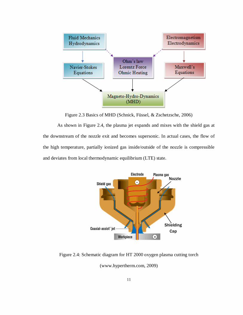
partially ionized gas will deviate from the LTE state significantly especially near the
electrodes and fringes of the arc column. Under such a condition called the Non-LTE, the
electron temperature will be much higher than the heavy-particle temperature. The
physics of the arc column is described by a magneto-hydrodynamic (MHD) model.

10
Figure 2.2: A thermal plasma discharge (Schnick, Füssel, & Zschetzsche, 2006)
The idea of MHD is that magnetic fields can induce currents in a moving
conductive fluid, which create forces on the fluid, and also change the magnetic field
itself. The set of equations which describe MHD are a combination of the Navier-Stokes
equations of fluid dynamics and Maxwell's equations of electromagnetism (see Figure
2.3). The electromagnetic equations are solved for fluids as well as solids. In the present
work, the sheath layers were not modeled.
11
Figure 2.3 Basics of MHD (Schnick, Füssel, & Zschetzsche, 2006)
As shown in Figure 2.4, the plasma jet expands and mixes with the shield gas at
the downstream of the nozzle exit and becomes supersonic. In actual cases, the flow of
the high temperature, partially ionized gas inside/outside of the nozzle is compressible
and deviates from local thermodynamic equilibrium (LTE) state.
Nozzle
Shielding
Cap
Figure 2.4: Schematic diagram for HT 2000 oxygen plasma cutting torch
(www.hypertherm.com, 2009)

12
A 2D Non LTE simulation of the heat transfer and flow patterns inside the nozzle
was carried out with a non-commercial computer code which could predict the
compressible effects of the thermal plasmas. The shield was not part of this simulation.
A non-uniform, body-fitted mesh was used for the 2-D modeling. A suitable
version of a non-commercial computer code FAST-2D (Flow Analysis Simulation Tool
of Two Dimensions) was employed to solve the set of partial differential equations with
the appropriate boundaries.
2.4 Governing equations
The governing equations along with the underlying assumptions are presented in
this section. As mentioned earlier a non-commercial computer code FAST-2D (Flow
Analysis Simulation Tool of Two Dimensions) by (Zhu, 1991) is used to solve this set of
governing equations for plasma modeling.
2.4.1 Basic assumptions
a. The plasma working gas used is either pure oxygen or a combination of oxygen
and nitrogen in the ratios 50:50, 20:80 or 80:20.
b. The plasma is in kinetic and chemical non-equilibrium state and separate
Maxwellian distributions of electrons and heavy particles exist.
c. Charge neutrality is sustained in the system provided that the plasma sheath near
the cold wall is ignored.
d. The viscous dissipation and pressure work terms in the energy equation are
neglected.

13
2.4.2 Continuity equation for species „s‟
where is the mass-averaged velocity of the gas, and are the number
density and number flux of species s, respectively, with the relationship (Li & Chen,
2001)
and
)
where , , and are the partial pressure, temperature, mass and electric
charge number of species s, respectively. is the externally applied electric field.
and are the ordinary and ambipolar diffusion coefficients for a multi-component gas,
respectively, with the following relationship (Li & Chen, 2001)
where
is the net production term of species s. For instance, consider O2, O++
and e as
the independent species undergoing following reactions.

14
The corresponding expressions for can be expressed as follows (Vincenti &
Kruger, 1965)
where is the coefficient appropriate to the backward reaction r (reactions (a)-
(c)). The superscript “*” indicates the values of number densities at chemical equilibrium
state. and represent the production rates of electrons in reaction (b) and (c),
respectively.
Then, the number densities of O and O+ can be calculated with the auxiliary
relationship
2.4.3 Momentum equation

15
where , and are the mass density, scalar pressure and viscous stress of the
gas, respectively. and are the current density and the self-induced magnetic field,
respectively.
2.4.4 Electron energy equation
where , , and are the mass density, specific enthalpy, thermal
conductivity and temperature of electrons, respectively. is the total electric field. is
the net radiation power per unit volume. is the rate of total energy change of
electrons resulting from elastic collisions with all heavy particles, which can be expressed
as
where is the average collision frequency between electrons and heavy
particles, which can be expressed as (Mitchner & Kruger, 1992).
where is the average momentum transfer cross section, is the mean relative
speed for particles with Maxwellian velocity distributions, which can be calculated by
(Mitchner & Kruger, 1992)
16
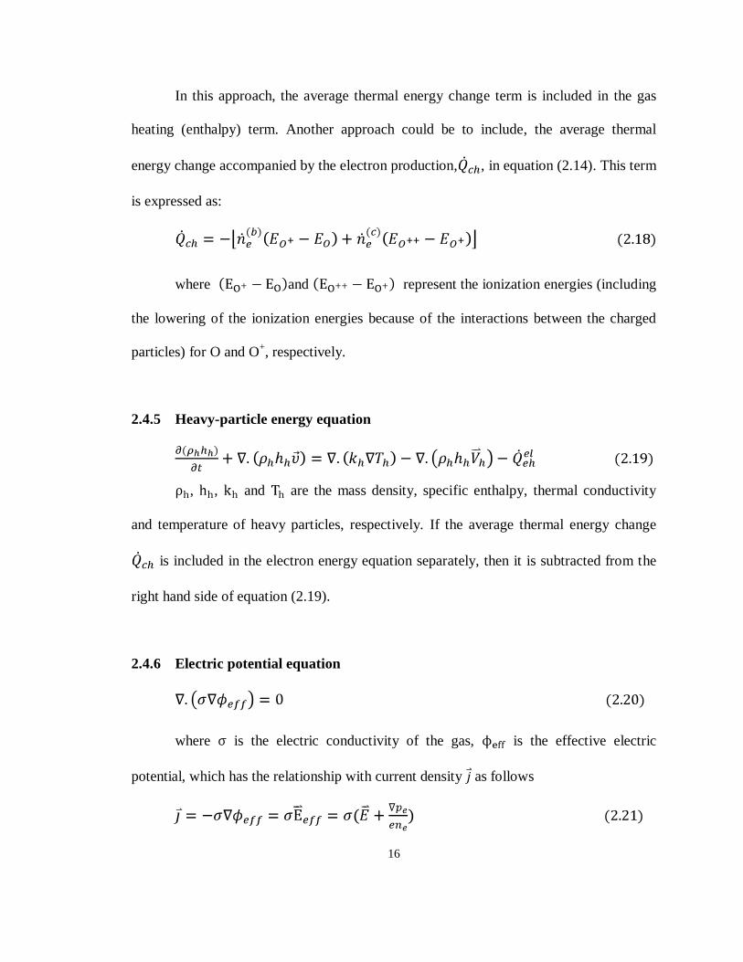
In this approach, the average thermal energy change term is included in the gas
heating (enthalpy) term. Another approach could be to include, the average thermal
energy change accompanied by the electron production, , in equation (2.14). This term
is expressed as:
where and represent the ionization energies (including
the lowering of the ionization energies because of the interactions between the charged
particles) for O and O+, respectively.
2.4.5 Heavy-particle energy equation
, , and are the mass density, specific enthalpy, thermal conductivity
and temperature of heavy particles, respectively. If the average thermal energy change
is included in the electron energy equation separately, then it is subtracted from the
right hand side of equation (2.19).
2.4.6 Electric potential equation
where is the electric conductivity of the gas, is the effective electric
potential, which has the relationship with current density as follows

17
2.4.7 Magnetic potential equation
where is the permeability in vacuum, is the magnetic vector potential
defined using the magnetic field as,
2.4.8 Terms in conservation equations
The explicit forms of various conservation equations are given in (Ghorui,
Heberlein, & Pfender, 2007). All the associated conservation equations have the generic
form as follows:
Figure 2.5: Generic form of conservation equations (Ghorui, Heberlein, &
Pfender, 2007)
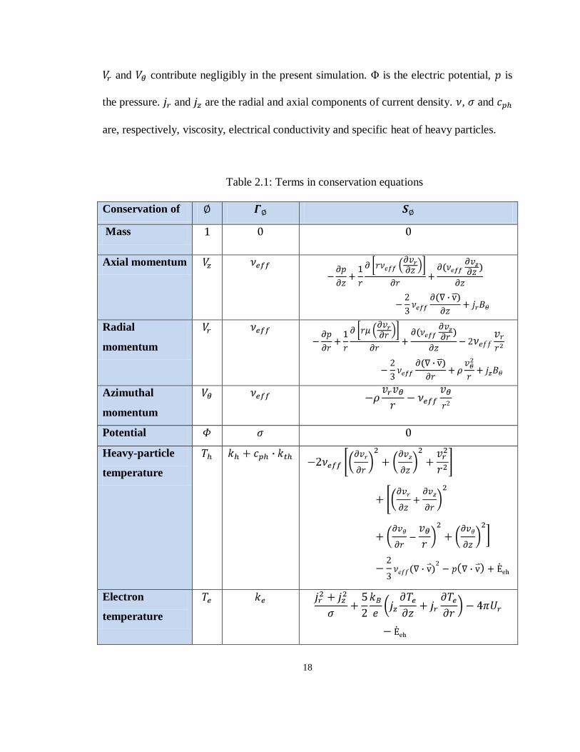
Table 2.1 describes the explicit forms of various conservation equations (Ghorui,
Heberlein, & Pfender, 2007). Some of the source terms involving
18
and contribute negligibly in the present simulation. Φ is the electric potential, is
the pressure. and are the radial and axial components of current density. , and
are, respectively, viscosity, electrical conductivity and specific heat of heavy particles.
Table 2.1: Terms in conservation equations
Conservation of
Mass
Axial momentum
Radial
momentum
Azimuthal
momentum
Potential
Heavy-particle
temperature
Electron
temperature

19
The self-induced magnetic field at radial location is computed integrating
as , where is the permeability of vacuum.
represents the energy transfer from electrons to heavy particles given by:
and .
where, and are, respectively, number density of electrons and heavy
particles. and are their respective masses. is the average volumetric collision
frequency between electrons and heavy particles. is the average thermal speed of
electrons and is the collision cross-section between electrons and heavy particles.
2.5 Boundary conditions
To specify the boundary conditions for pressure, velocity and other variables,
consider a typical computational domain like the one shown in Figure 2.5. It has
boundary conditions of the types: inlet, outlet, wall and symmetry.
Figure 2.6: A typical computational domain with boundary conditions (Li, Heberlein, &
Pfender, 2004)

20
A set of boundary conditions based on the Figure 2.5 for a typical torch with axial
injection is given in Table 2.1.
Table 2.2: A typical set of boundary conditions
Boundaries P (atm) u (m/s) v (m/s) w (m/s) T (K)
(Te and Th)
Φ (V)
BN
- 0 300
BCDG - 0 0 0 1000 0
GE - 0 0 0 3000
RF -
0
0
NOHR - 0 0 0
-
EF -
0
MLKR - - - - -
where, is derived from current density boundary
conditions and n represents the normal direction.

21
2.6 Property data
For the compressible flow and heat transfer simulations with oxygen-nitrogen as
the plasma working gas, tabulated pressure-temperature-dependent thermodynamic and
transport properties of oxygen plasmas in wide pressure and temperature ranges were
calculated with formerly developed computer code (Ghorui, Heberlein, & Pfender, 2007)
for the calculation of composition, thermodynamic and transport properties of
equilibrium/non-equilibrium oxygen-nitrogen plasmas.
Thermodynamic and transport properties were computed for a 17 species model
of nitrogen-oxygen plasma under different degrees of thermal non-equilibrium, pressures
and volume ratio of component gases. In the computation electron temperature ranged
from 300 to 45000K, mole fraction ranged from 0.8 to 0.2, pressure ranged from 0.1 atm
to 5 atm and thermal non-equilibrium parameter (Te/Th) ranged from 1 to 20. It was
assumed that all the electrons followed a temperature Te and the rest of the species in the
plasma followed a temperature Th. Compositions were calculated using the two
temperature Saha equation with appropriate energy level data and recently developed
collision integrals were used to obtain thermodynamic and transport properties. The
results were compared with published data under LTE conditions and an overall good
agreement was observed (Ghorui, Heberlein, & Pfender, 2006).
Linear interpolation was employed for computing the physical properties at
different gas pressures and temperatures. The radiation loss rate of oxygen plasmas (W/
m3) in the temperature range of 9000 K to 30000 K at atmospheric pressure was obtained
from experimental work (Gleizes & Cressault, 2007) and appropriate extrapolations were
applied along with suitable pressure dependence relations.

22
2.7 Features of FAST-2D
The governing equations described in earlier sections are solved by using the
FAST-2D solver with the following features.
Table 2.3: FAST-2D at a glance
Features Description
1 FAST-2D Flow Analysis Simulation Tool of 2-Dimension
developed by Zhu (1991) based on program by S.
Majumdar (1986), Institute of Hydromechanics,
University of Karlsruhe, Germany.
2 Discretization
technique
Finite volume
3 Grid type Non-orthogonal
4 Variable arrangement Non-staggered
5 Pressure velocity
coupling algorithm
SIMPLEC (Van Doormal and Raithby, 1984)
6 Scheme to avoid
oscillation faced with
non-staggered grid
arrangement
Rhie and Chow (1983) momentum interpolation scheme
7 Convection
differencing schemes
(a) hybrid /central/upwind ( Spalding, 1972)
(b) QUICK (Leonard, 1979)
(c) SMART (Gaskell and Lau, 1988)
(d) SOUCUP (Zhu and Rodi, 1991)
(e) HLPA (Zhu,1991)
8 Solution scheme (a) TDMA (alternate direction) of Thomas (Flecher,
1988).
(b) Strongly implicit procedure (Stone, 1968)
9 Turbulence k-epsilon (Launder and Spalding, 1974)

23
The general steps in FAST-2D for solving the governing equations with the
appropriate boundary conditions discussed in the former sections are given below. The
non-equilibrium thermodynamic and transport properties of oxygen-nitrogen plasma,
required to solve the governing equations are derived by (Ghorui, Heberlein, & Pfender,
2007).
1) Initialize all fields (p*, u*, v* etc.). “*” represents the initial/guessed value of any
variable.
2) Solve the u (axial) and v (radial) momentum equations using guessed pressure
field p*.
3) Solve the pressure correction equation (from the continuity equation) to get p‟
(pressure correction) field.
4) ; With the corrected pressure, correct the velocities and fluxes at the
cell centers and faces.
5) Solve the w.r (azimuthal) momentum equation for the swirling flows.
6) Solve the turbulence equations (optional)
7) Solve the enthalpy equation.
8) Solve the electron energy equation.
9) Solve the electric potential equation.
10) Solve the diffusion equation for electrons.
11) Solve the diffusion equation for ions.
12) Solve the heavy-particle energy equation.
24
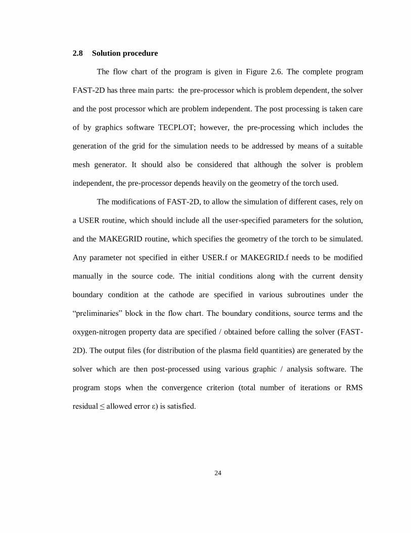
2.8 Solution procedure
The flow chart of the program is given in Figure 2.6. The complete program
FAST-2D has three main parts: the pre-processor which is problem dependent, the solver
and the post processor which are problem independent. The post processing is taken care
of by graphics software TECPLOT; however, the pre-processing which includes the
generation of the grid for the simulation needs to be addressed by means of a suitable
mesh generator. It should also be considered that although the solver is problem
independent, the pre-processor depends heavily on the geometry of the torch used.
The modifications of FAST-2D, to allow the simulation of different cases, rely on
a USER routine, which should include all the user-specified parameters for the solution,
and the MAKEGRID routine, which specifies the geometry of the torch to be simulated.
Any parameter not specified in either USER.f or MAKEGRID.f needs to be modified
manually in the source code. The initial conditions along with the current density
boundary condition at the cathode are specified in various subroutines under the
“preliminaries” block in the flow chart. The boundary conditions, source terms and the
oxygen-nitrogen property data are specified / obtained before calling the solver (FAST-
2D). The output files (for distribution of the plasma field quantities) are generated by the
solver which are then post-processed using various graphic / analysis software. The
program stops when the convergence criterion (total number of iterations or RMS
residual ≤ allowed error ε) is satisfied.

25
Figure 2.7: Flow chart for NEQ code
The variables used in FAST-2D and the subroutines in the non-equilibrium
plasma code along with their purpose, are listed in appendices A and B.
26
3. GRID GENERATION
3.1 Introduction
The original pre-processor of the FAST-2D solver did not have an inbuilt finite
volume grid generator fitting the torch geometry. Since the grid plays the most important
role in getting a converged solution, a flexible grid generator is extremely necessary. This
section describes a general routine developed to serve this purpose, its limitations and the
improvements made to overcome these limitations.
The older version of the grid generator program required 23 measured dimensions
of the plasma torch as an input whereas the new version requires 28 of those. These
dimensions are usually readily available from the engineering drawings of the plasma
cutting torches. Once the dimension data are entered, the geometry is specified and the
program then divides the torch geometry into various computational zones as described in
the subsequent sections. The number of grid points in each zone and the choice of grid
spacing distribution style are specified by the user. With these inputs taken from the user,
the code generates a complete grid with the help of the zone boundary equation
subroutines and the grid generator functions GRD, GRDC and GRDR described later in
this chapter.
The torch geometry and computational mesh used to describe the fields in it are
specified in the routine MAKEGRID.f. This routine allows the specification of the torch
geometry based on the use of “control nodes” and “zones”, as depicted in figures given
later in this chapter. The geometry generated by MAKEGRID.f includes, apart from the

27
fluid region inside the torch, the solid regions (i.e. cathode, nozzle, etc.) and a part of the
outside of the torch.
3.2 Old grid generator
3.2.1 Control points of the plasma torch geometry
The older version of the grid generator required 23 dimensions needed to be
measured for the considered torch as illustrated in Figure 3.1. Bars associated with each
wn and hn dimensions indicate the lengths to be measured.
Figure 3.1: Control points and dimensions of plasma torch geometry in older version of
grid generator (Ghorui, Heberlein, & Pfender, 2007)

28
3.2.2 Coordinates extracted from the dimensions
The derived coordinates for the chosen example are:
Table 3.1: Control points‟co-ordinates
Control Point X-Coordinate Y-Coordinate
A XA = 0 YA = 0
B XB = 0 YB = W4
C XC = 0 YC = W1
D XD = 0 YD = W1+W2
E XE = 0 YE = W1+W2+W3
F XF = (H7-H8) YF = 0
G XG = XF YG = W4
H XH = H4 YH = W6
I XI = H4 YI = W6+W5
J XJ = H4 YJ = YE
K XK = H6 YK = 0
L XL = H6 YL = W6
M XM = H6 YM = DERIVED POINT*
N XN = H6 YN = DERIVED POINT
O XO = H7 YO = 0
P XP = H7 YP = W7
Q XQ = H7 YQ = W8
R XR = H7 YR = DERIVED POINT
S XS = H7 YS = DERIVED POINT
T XT = H3 YT = 0
U XU = H3 YU = DERIVED POINT
V XV = H3 YV = W1+W2+W3/2.
W XW = H5 YW = 0
X XX = H5 YX = W9
Y XY = H5 YY = DERIVED POINT
Z XZ = H9 YZ = 0
AA XAA = H9 YAA = W10
BA XBA = H9 YBA = DERIVED POINT
CA XCA = H2 YCA = 0
DA XDA = H2 YDA = W11
EA XEA = H2 YEA = W12
FA XFA = H1 YFA = 0
GA XGA = H1 YGA = W13
HA XHA = H1 YHA = W14
*Note: “Derived Points” are obtained using the zone boundary functions

29
After extracting the control points from the torch drawing, the solid and fluid zone
boundaries are derived from the defined boundary functions. The resulting frame for grid
generation is shown in Figure 3.2.
Figure 3.2: Frame for grid generation with zone boundaries (Ghorui, Heberlein, &
Pfender, 2007)
3.2.3 Zones in radial direction (X-zones)
The zones created are dependent on the geometric features of the torch and are
chosen to ease the setting of the boundary conditions. In the older version of the
geometry subroutine, zone-2 was shaped to handle the hafnium insert in the cathode.
Zone-3 handled the surface condition of the cathode tip; zone-4 modeled the nozzle exit
and zone-5 handled the outflow zone. Also, five different grid distributions could be
chosen in five different zones described above. These X-zones are shown in Figure 3.3.

30
Figure 3.3: Zones in radial direction (X-zones) (Ghorui, Heberlein, & Pfender, 2007)
3.2.4 Zones in axial direction (Y-zones)
Similar to the case of X-zones, the Y-zones were chosen to specify the boundary
conditions easily. Zone-1 handled the hafnium insert, zone-2 handled the cathode surface,
zone-3 consisted of gas flow region, and zone-4 handled the nozzle wall. Zone-5 was the
plasma formation and expansion zone. Zone-6 covered part of the nozzle wall and
outflow zone. Zone-5 and zone-6 did not require grid number and style specifications as
they were dependent on the specifications set in zone-1 to zone-4.
Four different grid distribution types were chosen for four different zones up to
the cathode tip and then only two different types of grid distributions were chosen for the
domain downstream as shown in Figure 3.4.

31
Figure 3.4: Zones in axial direction (Y-zones) (Ghorui, Heberlein, & Pfender, 2007)
3.2.5 Zone boundary functions
Figure 3.5: Zone boundary functions (Ghorui, Heberlein, & Pfender, 2007)

32
Functions were developed to extract equations for boundaries of every zone.
These functions, as shown in Figure 3.5, computed the equations for the zone boundaries.
For a given x-coordinate, boundary functions gave the y-coordinate at a particular zone
boundary. Once all the boundaries were obtained, the next step was to discretize the
lengths with optimum grid density at associated regions.
3.2.6 Functions employed for generating grids of varying densities
Figure 3.6: Example of varying density grid (Ghorui, Heberlein, & Pfender, 2007)
In the above example, a range „R‟ is discretized by „N‟ grid points such that the
distance between consecutive nodes is a factor „f‟ of the distance between the previous
set of consecutive nodes.
Therefore,
That is

33
For f<1 we have an outward contracting grid and for f>1, we have an outward
diverging grid. A few examples of varying-density grids are presented below. For f=1,
the function needs special care due to 0/0 form.
Function GRD(f,r,n) generates grid points of following types:
Figure 3.7: Varying density grid asymetric about the center (Ghorui, Heberlein, &
Pfender, 2007)
Function GRDC(f,r,n) generates grid points of following types:
Figure 3.8: Varying density grid symmetric about the center (Ghorui, Heberlein, &
Pfender, 2007)
Function GRDC(f,r,n) uses the Function GRD(f,r,n) in the first and the second
half of the points in an order opposite to each other. Function GRDR(r,n) generates grid
points when the ratio of the interval between consecutive grid points and the range is
given. This is particularly advantageous in the zone where a number of zones of different
styles merge into a single zone. This function has been used in the zone following the
cathode tip.

34
The x-coordinates and the y-coordinates are derived using the functions discussed
above as shown in Figures 3.9 and 3.10 respectively
Figure 3.9: Assigning x-coordinates using the grid density functions (Ghorui, Heberlein,
& Pfender, 2007)
Figure 3.10: Assigning y coordinates using the grid density functions (Ghorui,
Heberlein, & Pfender, 2007)

35
3.2.7 Geometric limitations in FAST-2D and MAKEGRID
The complete geometry of all Hypertherm torches could not be modeled using the
earlier version of the MAKEGRID.f file, because this file only allowed the specification
of a geometry using 23 control dimensions. Furthermore, it did not allow the
specification of the nozzle counter-bore, the cone at the torch exit and the vent flow.
Also, the parameters specified in MAKEGRID are “hard-wired” into the rest of the
FAST-2D solver. The swirl injection radius could not be specified in the USER routine,
nor was it specified explicitly in the MAKEGRID routine. The approach used previously
for considering the location of the swirl gas injection, consisted of assigning it to a given
node in the mesh, describing the inlet of the flow injection point – this is done in the
BOUNDS.f file (the file where part of the boundary conditions are specified). This
approach made the swirl injection radius mesh-dependent; therefore non-flexible and
unreliable. Moreover, the size of the gas injection holes could not be specified in the
MAKEGRID.f file. This section addresses the work done towards improving these
aspects of the user-specified part of the FAST-2D code.

36
3.2.8 Current geometry/mesh-generation routine
The above limitations of the MAKEGRID.f routine arise from the fact that the
generated mesh is structured, having the axis of the torch as the driven direction, and uses
a fixed amount of control points.
Apart from the above limitations, an even more important issue for the use of
FAST-2D for the modeling of the Hypertherm HT4400And vented 400A process plasma
torches is that the MAKEGRID.f file is tightly coupled to several routines in FAST-2D.
These files are not only the files used for the definition of the boundaries of the domain
and boundary conditions, but also to the routines in the “problem-independent” part of
the code. Therefore, any modification of the MAKEGRID.f file needs to be consistent
with not only the boundary specification and boundary conditions files, but also with all
the routines in FAST-2D that rely on the specific form of MAKEGRID.f.
Therefore, in order to use FAST-2D to simulate the new generation cutting
torches by Hypertherm Inc., the file MAKEGRID.f needed to be modified/rewritten, as
well as all the routines in FAST2D that rely on the parameters used in MAKEGRID (e.g.
for the NEQ code, the routines MAIN.f, BOUNDS.f, FILES_SPEBND.f,
INITIA_CURRENT.f, OVACON.f, SETJ.f, SOURCE.f).

37
3.3 New geometry/mesh-generation routine
To simulate the HT4400 400A O2 and vented 400A process cutting torches, the
file MAKEGRID.f was missing the following features:
1. Location and size of the swirl injection.
2. Counter-bore or conical expansion at the nozzle outlet.
3. Vent flow channel.
The new MAKEGRID routine was based on the geometrical specifications
depicted in Figure 3.11 According to Figure 3.11, each boundary of the computational
domain (cathode, nozzle inside, etc.) is determined by a set of control points. The torch
geometry is given by 4 profiles: the insert (i), cathode (c), nozzle inside (n), and nozzle
outside (t). Each one of these profiles is specified by a set of “control points” (i.e. for the
cathode profile, the points 1c, 2c, and 3c).
Figure 3.11: New geometry/mesh-generation specification for the file MAKEGRID.f
One disadvantage of the geometry specification given in Figure 3.11 is that the
vent flow channel has to be modeled as vertical. This is due to the structured nature of the

38
mesh generation routine, consistent with the capabilities of FAST-2D. Furthermore, the
shield flow channel cannot be included. Addition of the shield gas flow will require
further modification of the MAKEGRID routine. Table 3.2 shows a summary of the
current and new number of control points used in MAKEGRID.f for the specification of
the torch geometry.
Table 3.2: Comparison between old and proposed geometry/mesh-generation routine
Number of “control-
points”
Old New
Insert 2 2
Cathode 3 3
Swirl injection 0 2
Nozzle inside 6 10
Torch 4 4
TOTAL: 15 21
3.4 Summary of features of new mesh generation routine
1. The new MAKEGRID.f routine allows the specification of axial, radial, and
tangential gas injection, and/or combinations of these.
2. The new routine is able to describe the geometry of the vent channel. (The old
MAKEGRID.f routine lacked an extra “control point” to allow the specification of
the vent channel design).
3. The new routine allows the correct specification of the geometry of the nozzle exit,
e.g. counter-bore and/or conical expansion.

39
4. The new MAKEGRID.f routine has the option, available in the original routine, to
allow the simulation of the domain outside the torch (plasma jet) and the work piece.
5. The new routine is in a modular and user-friendly manner. This modularity makes the
modification of the geometry specification (i.e. addition/removal of control points)
straightforward and intuitive in order to accommodate future torch designs.
The new MAKEGRID routine is developed with “modularity” as the main goal.
The new routine divides the spatial domain of the torch in “characteristic zones” along
the X and Y axes. The X- and Y-zones currently considered in the new MAKEGRID.f
routine are depicted in Figure 3.12. Each zone encompasses several “control points”
along a given axis; i.e. in the X-zones plot in Figure 3.12, zone 4 contains 5 “control
points”: points 11 to 15. Therefore, the definition of “zones” along the X-axis is
somewhat arbitrary, as they are specified to allow identification of particular regions of
the domain for imposition of the boundary conditions. As an example, X-zone 2 is
included to specify the boundary conditions for the radial gas injection, whereas X-zone 6
allows the specification of the vent channel.

40
3.5 New X- and Y- zones
Figure 3.12: Zones along the x (top) and y (bottom) coordinates used to characterize
general plasma torch geometries

41
The mesh generation routine consists of creating a quasi-orthogonal sub-mesh in
each quadrilateral region delineated by the dashed lines in the Y-zones plot. The main
objective of the new MAKEGRID.f routine is to create a sub-discretization of each
quadrilateral sub-region given by the intersection of the sets of dashed lines in the Y-
zones plot in Figure 3.12. That is, every quadrilateral region in this plot will be further
divided into a user-specified number of grid nodes along the X- and Y-axis. The
modularity of the new MAKEGRID.f routine will allow the addition or removal of any
number of “control points” in a consistent manner, such that the domain will still be
divided into quadrilateral sub-regions, which are subsequently discretized. The flow chart
for grid generation subroutine is given in Figure 3.13. The factors FX1 to FX9 and FY1 to
FY7 are the factors deciding the variations in grid densities.
Figure 3.13: Flow chart for grid generation subroutine
NX=NX1+NX2+…+NX9-8 NY=NY1+NY2+…+NY7-6
SET NX1 TO NX9 SET NY1 TO NY7
GRD(f,r,n)GRDC(f,r,n)GRDR(f,r,n)
BOUNDARY FUNCTIONS
X-COORDINATES
Y-COORDINATES AND COMPLETE MESH
GEOMETRY DEFINITION
DERIVATION OF ZONES AND CONTROL POINTS
SET FX1 TO FX9 SET FY1 TO FY7
GRD(f,r,n)GRDC(f,r,n)GRDR(f,r,n)

42
3.6 Sample grids generated by the grid generation subroutine:
Figure 3.14: Grid for HT2000 (200A O2/air process)
Figure 3.15: Grid for HT4400 (400A O2/air process)

43
Figure 3.16: Grid for vented torch (400A O2/air process)
The sample grids generated by the modified grid generation subroutine are
shown in Figures 3.14 (for HT2000 torch), 3.15 (for HT4400 torch) and 3.16 (for 9427
O2 Rev 1 torch). Various solid/fluid zones are shown in different colors. As emphasized
by the diagrams, the modified grid generator features the ability to input axial injection
zone, vent flow zone and nozzle exit counter bore or cone.

44
4. MODELING OF RADIATION LOSSES
4.1 Introduction
It has been observed that the radiation model has a significant effect on the
distribution of plasma field quantities and therefore it is required to select an adequate
radiation model in order to produce reasonable results. In the code, the radiation losses
are modeled by the total effective volumetric radiation loss term. Such an approximation
is widely employed in the thermal plasma community.
In this concept, self-absorption by the plasma is taken into account by assuming a
plasma-geometry and solving the radiation transport for this assumed geometry. The
geometry dependence is expressed in the terms of an effective radius of the radiating
volume. If the effective radius Reff = 0.0 mm, there is no self-absorption and all radiation
escapes. For increasing values of Reff, some of the radiation is absorbed in the arc itself.
4.2 Energy transport in thermal plasmas
The thermal non-equilibrium feature expresses the transport of thermal energy by
the two-temperature model. Two-temperature models do not assume that the electrons
and the heavy-species in the plasma equilibrate instantaneously; therefore they allow
partial kinetic equilibration and hence model the energy transport processes within the
plasma flow more accurately than a single temperature model. The energy conservation
equations solved in FAST-2D are of the form (Boulos, Fauchais, & Pfender, 1994):
(4.1)

45
The terms composing these equations are displayed in Table 4.1.
Table 4.1: Terms in the thermal energy conservation equations
Variable Transient Advection Diffusion Reaction
hT
t
hh hhu
hq'
ehQ
eT
t
he ehu
eq'
rJeh QQQ
In Table 4.1, Th = Heavy-species temperature
Te = Electron temperature
hh = Heavy-species enthalpy
he = Electron enthalpy
ρ = Mass density
u = Velocity
q’ = Total effective heat flux (due to the transport of translational
energy and species enthalpy by diffusion)
Qeh = Net energy exchange term (explicit coupling between the energy
equations)
QJ = Joule heating
Qr = Net volumetric radiation loss term

46
4.3 Net volumetric radiation loss
It is crucial to model the transport of radiative energy in a thermal plasma flow
adequately in order to describe the plasma flow dynamics correctly. This term can
especially dominate the energy transport at very high temperatures (i.e. temperatures
greater than ~ 30000 K). Fundamentally, the net volumetric radiation density, which is
the net energy emitted per unit volume and time, can be expressed by:
(4.2)
where = radiative flux
= vector of spatial coordinates
= spectral absorption coefficient
= Planck function for a black body
(4.3)
where = speed of light
= Planck constant
= Boltzmann constant.

47
The integration for in (4.2) is over all frequencies , all directions and over
all sources on the ray from the domain boundary ( ) to the point under
consideration. Expressions (4.2) and (4.3) indicate that is a complex function of the
geometry containing the plasma flow and the local properties of the plasma.
4.4 The effective volumetric radiation loss approximation
In plasma flow simulations, the modeling of the radiative transfer given by (4.2)
represents an exceedingly large effort (i.e. the number of calculations needed scales with
the cube of N, the number of grid nodes (N3)). The dominant approach used in the
thermal plasma community to approximate the radiative energy exchange consists of the
radiative transport model developed by (Lowke, 1974). Lowke‟s approach consists of
modeling all radiation as being emitted in the center of an isothermal sphere with a
characteristic effective radiation radius . Radiation can be reabsorbed only within
this sphere. Therefore, radiation emitted in the arc has to pass through a certain distance
of (not optically thin) plasma before escaping to the walls. By assuming that the sphere is
isothermal and by assigning it a radius, three independent variables in equation (4.2) are
removed, giving a total volumetric radiation term that depends only on the local
temperature.
Lowke‟s model has some weaknesses, especially when considering that the arc
must be given a characteristic radiation radius. Also, a plasma flow can have areas in the
outer part where the absorption of radiation from the inner parts is higher than the emitted
radiation, effectively giving a negative radiation loss. On the other hand, Lowke‟s model

48
provides a consistent and practical way of determining the radiation loss from thermal
plasma, suitable for numerical simulation.
By assuming the spectral absorption and Planck function to be constants
and integrating from to over all angles in equation (4.2), the net volumetric
radiation loss is given by:
(4.4)
Here, is the net emission coefficient, which is a function of the plasma gas, the
local temperature and the effective absorption radius (a model parameter). It is this
net emission coefficient which approximates locally the radiative energy transfer from
the plasma to its surroundings.
Lowke‟s model was originally derived for thermal plasmas in thermal equilibrium
(i.e. ). For a thermal non-equilibrium plasma model, and considering that
radiation depends mostly on the population of excited species and these, in turn depend
primarily on the electron temperature, the expression given by (4.4) is evaluated as a
function of the electron temperature (i.e. ).

49
Figure 4.1: Effective net radiative emission coefficient for oxygen as a function of
temperature: data previously used in FAST-2D (Krey & Morris, 1970), and new radiation
data by (Gleizes & Cressault, 2007) for two effective absorption radii (Reff = 0.0 & 0.5
mm)
The radiation model employed earlier used radiation data for oxygen plasma
obtained by (Krey & Morris, 1970). The experimental data as reported by Krey and
Morris span over temperatures in the range between 9000 and 14000 K. This data was
curve-fitted and extrapolated and specified in the file O2RAD.DAT.
Figure 4.1 shows the radiation data previously used in FAST-2D (extrapolations
of the data from Krey and Morris) and the radiation data calculated by (Gleizes &
Cressault, 2007) for oxygen plasma for two representative effective radii:
(optically thin) and

50
Figure 4.2: Effective net radiative emission coefficient for oxygen as a function of
temperature (T) and effective absorption radius (Reff) for 1 atm (Gleizes & Cressault,
2007)
Figure 4.2 shows the net emission coefficient Reff for oxygen plasma as a function
of temperature for different effective absorption radii. The data was provided by A.
Gleizes and Y. Cressault from the Université Paul Sabatier, France. The “optically thin”
assumption corresponds to .
Due to the small volume in which the plasma is contained inside a cutting torch, it
is reasonable to assume that all emitted radiation leaves the plasma without further re-
absorption (i.e. the optically thin assumption). Nevertheless, the two values of the net
emission coefficient ( (optically thin) and ) have been
used in simulations of the plasma torches to observe the sensitivity of the flow
characteristics to the radiation transfer model, as discussed in the next sections.

51
It also needs to be considered that the calculation of the net emission coefficient
depends on the plasma composition, which is not only a function of temperature, but also
of pressure. It is reasonable to assume that radiation losses typically increase
approximately linearly with pressure. The radiation data provided by Gleizes and
Cressault have been calculated for a pressure of 1 atm. The fact that the pressure inside
the cutting torch changes drastically (i.e. from 4 atm to 1 atm), the radiation correction is
applied in the following manner (Hsu & Pfender, 1983):
Here, and ( are radiation loss terms and and are the
corresponding pressures.
4.5 Cutting torch energy balance
The total amount of energy lost by radiation per unit time Pr can be calculated
according to:
(4.6)
Here, V represents the volume of the spatial domain. The relative importance of
the radiation loss with respect to the net energy balance is given by the fraction of energy
r lost by radiation:
where, Pin is the input power, I the total current, and ΔΦ the total voltage drop
across the torch. The values of the quantities Pr, Pin and r for the two simulations of one

52
of the 400A torches of Hypertherm (HT4400) are presented in Table 4.2. The radiation
loss term in the case of optically thin plasma assumption is greater than that in the case of
the plasma with Reff = 0.5 mm assumption owing to the higher emission coefficients in
the former case.
The net power loss by radiation represents a very small fraction of the total power
input as shown by the results in Table 4.2. In reality, it is observed that the plasma flow
fields are heavily dependent on the radiation model used in spite of seemingly
contradicting results in the table. There is indeed no contradiction: the precise form of the
energy transfer affects drastically the characteristics of the plasma flow. However, due to
the small volume of the plasma, the integration of the net emission coefficient over the
plasma volume sums up to a very small quantity of power loss when compared with the
net amount of power that goes into the plasma. Furthermore, the net energy balance
depends on the global conservation of energy, which is not very sensitive to the precise
configuration of the plasma flow field (i.e. for the global energy balance what matters are
not the profiles of the plasma characteristics, but their integral value).
Table 4.2: Energy balance in a plasma torch
Effective Absorption Radius
Reff = 0.0 mm (optically thin) Reff = 0.5 mm
Total Volumetric
Radiation Loss: Pr
Power input: Pin
Fraction of power lost
by radiation: r = Pr/Pin

53
Figure 4.3 presents the electron temperature distributions inside the torch as well
as the distribution of the net emission coefficient for one of the torches studied (results
displayed in later chapters). The net emission coefficient has a marked dependence on the
electron temperature. This dependence causes the distribution of net emission coefficient
to be highly localized, which limits the extent of the volume V in the expression for total
energy lost by radiation given by equation (4.6).
Figure 4.3: Temperature and emission coefficient distribution in the HT4400 torch. Top
row: electron temperature distributions (left, Reff = 0 mm; right Reff = 0.5 mm). Bottom
row: net emission coefficient (left, Reff = 0 mm; right Reff = 0.5 mm) (Trelles, Heberlein,
& Pfender, 2007)

54
5. EFFECT OF CATHODE CURRENT DENSITY BOUNDARY CONDITION
5.1 Introduction
The model requires a current density profile as one of the boundary conditions.
The emitting part of the cathode is a hafnium rod inserted in a copper support. There are
different options for determining current density at the cathode surface. One of the
alternatives is to use an experimentally measured temperature profile along with the
Richardson-Dushman equation (Boulos, Fauchais, & Pfender, 1994).
When a cathode is heated to a sufficiently high temperature, electrons are emitted
with a current density j given by the Richardson-Dushman equation:
where A is a constant having a value of about for most
metals, T the surface temperature in Kelvin, e the thermionic work function of cathode
surface, e the electron charge and kB Boltzmann's constant. As known from the equation
(5.1), the current density of thermionic emission is highly sensitive to the cathode surface
temperature. Unless the temperature is increased to a sufficiently high value, it is not
possible to reach the current densities which are encountered in the plasma arcs.
This can be clearly seen when the Richardson-Dushman equation is plotted to
express the relationship between the electrode surface temperature and the current density
emitted from the electrode for various thermionic work functions of the electrode
material as shown in Figure 5.1.

55
Figure 5.1: Cathode current density vs. electrode temperature for various work
functions (Zhou & Heberlein, 1998)
For the high temperature zone, the current density goes up rapidly as the
thermionic work function increases. On the contrary, for lower temperatures the curves
for different thermionic work functions merge together. For a particular thermionic work
function, the current density has the peak value at the maximum electrode temperature
and then decays exponentially as the temperature decreases.

56
5.2 Initial profile used for the simulation
It is not straight forward to evaluate the current density distribution from the
Richardson- Dushman equation directly because the thermionic work function of cathode
material and the temperature distribution of the electrode surface may not be specified
clearly. Hence, another option of using an experimentally determined current density
profile seems more convenient.
The initial approach was to assume that the current density distribution on the
hafnium insert surface was uniform (Li, Heberlein, & Pfender, 2004):
where, I is the arc current and Ac is the area of the hafnium insert frontal surface.
Based on experimental measurements, a more realistic profile was used in the modified
versions of the code as described in the following sections.
Another approach involving conservation of current is to employ an
experimentally observed profile shape in front of the cathode and to adjust its parameters
in order to conserve the total current. Current density in the method using Richardson-
Dushman equation depends on the assumed temperature over the cathode surface in
which computational difficulty in reaching appropriate temperatures may result in
inappropriate current densities affecting the ultimate distributions of temperature and
other plasma quantities. In the current version of the code, the shape of the current
density profile over the cathode surface is derived from a spectroscopic measurement of
the temperature in front of the cathode for an arc current of 200A.
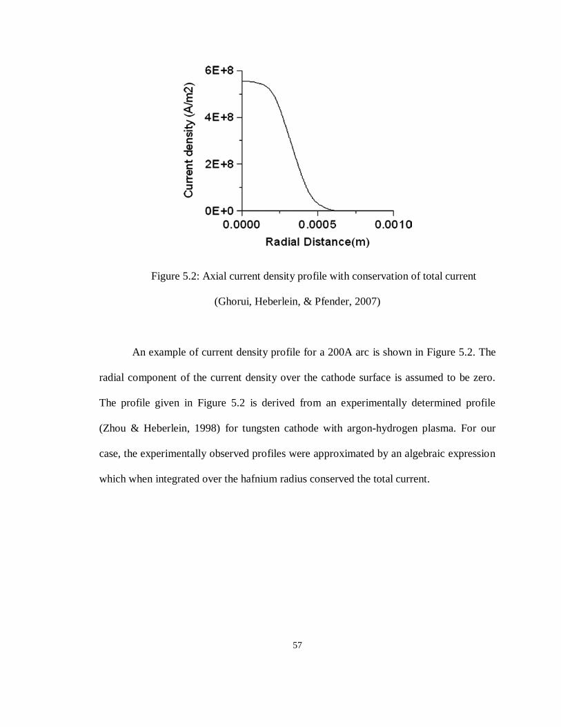
57
Figure 5.2: Axial current density profile with conservation of total current
(Ghorui, Heberlein, & Pfender, 2007)
An example of current density profile for a 200A arc is shown in Figure 5.2. The
radial component of the current density over the cathode surface is assumed to be zero.
The profile given in Figure 5.2 is derived from an experimentally determined profile
(Zhou & Heberlein, 1998) for tungsten cathode with argon-hydrogen plasma. For our
case, the experimentally observed profiles were approximated by an algebraic expression
which when integrated over the hafnium radius conserved the total current.

58
5.3 Effect of current density boundary condition at cathode
The current density distribution plays a huge role in the realized temperature
distribution. In practice, a converged solution could be obtained for any current density
by specifying an appropriate grid distribution. Improper grid density in the nozzle section
makes the code diverge as the constriction tears apart the flow.
This problem becomes severe with higher which is the case for 400A torches.
Due to the scarcity of available experimental data related to current density profiles at the
cathode for 400A torches, different profiles were tried as boundary conditions in the
simulation. The axial current density profiles were obtained conserving the total current
of 400A while maintaining a similar profile shape as that for a 200A torch. The radial
component of the current density over the cathode surface is assumed to be zero. The
results are presented later.
The current density profile over the cathode as described above is given by the
equation , where c is a constant which determines the width of the profile
(Ghorui, Heberlein, & Pfender, 2007). and are the maximum current density at the
center and the radius of the hafnium insert respectively. The value of c used for HT2000
torch simulation was 2.8. Figure 5.3 is a plot of a range of profiles used in the simulation.

59
Figure 5.3: Various axial current density profiles used as boundary condition at cathode
where c is constant in equation for profiles given by
5.4 Simulation results with various current densities for Reff = 0.5 mm
Figure 5.4: Temperature profiles at the nozzle exit in HT4400 torch for the current
density profiles given in Figure 5.3

60
Figure 5.4 shows the corresponding nozzle exit temperatures for the profiles given
in Figure 5.3. As expected, the peak temperatures are higher for narrower current density
profiles at the cathode. Although a converged solution was obtained for the narrowest
profile (c = 2.8), the maximum temperatures inside the torch are unrealistically high.
Such high temperatures would imply strong radiation that could not be sustained by the
power input to the torch. These exceedingly high temperatures indicate the necessity of
using Reff = 0.0 mm (optically thin plasma assumption) for this profile.
Simulation of HT4400 torch with different current density profiles at the cathode
suggests that this boundary condition plays an important role in determining the plasma
solution fields. This also emphasizes the need for experimental data to validate the used
current density boundary condition specified at the cathode for a 400A cutting torch.
Table 5.1 summarizes the simulation results for various combinations of current
density profiles and effective radii of radiation in the HT2000 and HT4400 torches.
Figure 5.4 and Table 5.1 indicate a discrepancy in the results for which
might be because of the grid sensitivity of the code. In Table 5.1, as the value of c in the
equation for the cathode current density profile increases, that is the current density
profile becomes narrower, higher peak temperatures at the cathode and the nozzle exit are
observed. The disagreement with the stated observation, of the results for could
be explained as follows. The NEQ plasma code is highly grid sensitive. Every simulation
of the code needs an optimized grid in order to get converged results. The simulations
with different current density boundary conditions required different grids optimized for
every current density profile used. It was observed that the flat zones in the exit
temperature profile for in Figure 5.4 were due to changed grid density in that
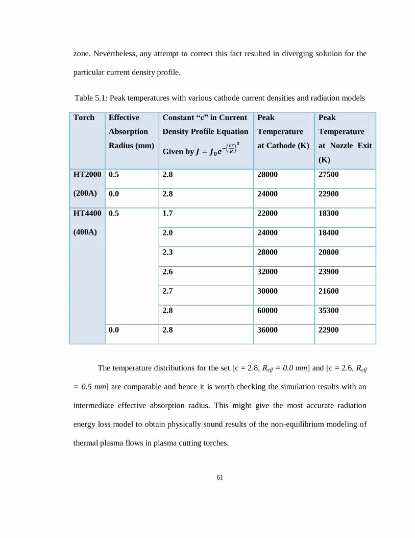
61
zone. Nevertheless, any attempt to correct this fact resulted in diverging solution for the
particular current density profile.
Table 5.1: Peak temperatures with various cathode current densities and radiation models
Torch Effective
Absorption
Radius (mm)
Constant “c” in Current
Density Profile Equation
Given by
Peak
Temperature
at Cathode (K)
Peak
Temperature
at Nozzle Exit
(K)
HT2000
(200A)
0.5 2.8 28000 27500
0.0 2.8 24000 22900
HT4400
(400A)
0.5 1.7 22000 18300
2.0 24000 18400
2.3 28000 20800
2.6 32000 23900
2.7 30000 21600
2.8 60000 35300
0.0 2.8 36000 22900
The temperature distributions for the set [c = 2.8, Reff = 0.0 mm] and [c = 2.6, Reff
= 0.5 mm] are comparable and hence it is worth checking the simulation results with an
intermediate effective absorption radius. This might give the most accurate radiation
energy loss model to obtain physically sound results of the non-equilibrium modeling of
thermal plasma flows in plasma cutting torches.

62
6. RESULTS AND DISCUSSION
6.1 Simulation of HT2000 200A O2/Air cutting torch
6.1.1 About the torch (www.hypertherm.com, 2009)
A section of HT2000 torch along its axis is shown in Figure 6.1. The dimensions
and other parameters for the grid generation are obtained on the basis of this drawing.
Figure 6.1: Schematic of HT2000 torch (dimensions in mm) (Li, Heberlein, &
Pfender, 2005)

63
In the schematic diagram of the Hypertherm HT2000 200A O2/Air plasma cutting
torch shown in Figure 6.1, the geometrical sizes are based on the drawings of the product
and the object measurements. The emitting part of the cathode is hafnium, while the
supporting part is copper. The nozzle and the shielding part are also made of copper.
6.1.2 Process parameters
The actual simulation domain used for the modeling is shown in Figure 6.2. The
shaded portions represent the solid parts whereas the un-shaded ones correspond to the
fluid domain.
Figure 6.2: Simulation domain (dimensions in mm) (Li, Heberlein, & Pfender,
2005)

64
Table 6.1: Steady state process parameters and torch specifications (200A torch)
Flow rate of O2 (79.6 scfh)
Plasma plenum pressure (54.96 psig)
Torch current 200A
Swirl injection type Axial
Swirl angle 20
Number of swirl injection holes 20
Diameter of swirl injection holes (0.025”)
Table 6.1 illustrates a few important process parameters and specifications of the
HT2000 torch. Corresponding code parameters are given in Table 6.2. These parameters
are specified in the USER.f file.
Table 6.2: Steady state parameters converted to code parameters (200A torch)
TCRN 200 (A)
TAND 600 (K)
TIN 300 (K)
UIN 21.2416 (m/s)
WIN 7.7313 (m/s)
PRSIN 480280.5 (Pa)
In Table 6.2, TCRN denotes the total torch current, TAND is the nozzle wall
temperature, and TIN, UIN, WIN and PRSIN denote the inlet- temperature, axial
velocity, tangential velocity and pressure respectively. The velocities are calculated from
the flow rate as described in the following section.

65
6.1.3 Input velocity calculations from inlet flow rate
The inlet velocity components to be specified in USER.f subroutine are calculated
from the flow rate specification as follows. The flow rate in (standard cubic feet per
hour) is first converted to a flow rate in using the inlet pressure and temperature
using the ideal gas law. The velocity ( is calculated from the flow rate in by
division by the area of inlet.
Converting standard flow rate for inlet conditions using ideal gas law:
Area of inlet:

66
Now, the dimension of the inlet zone needs to be calculated in order to be
specified in the grid generation subroutine. This dimension is the width of the annulus
with its area equal to the total area of the swirl injection holes.
Dimensions of inlet zone:
6.1.4 Generated Grid
The grid generated by the modified grid generator is shown in Figure 6.3.
Figure 6.3: Mesh for HT2000 torch

67
6.1.5 Initial simulation results
The validity of the results of FAST-2D when compiled with the modified version
of the grid generator and radiation model based on the data by Gleizes et al with optically
thin assumption; using Intel Fortran Compiler version 10 has been tested by re-running
the simulation of the cutting torch HT2000 operating with pure oxygen and a total current
200A (HT2000 200A O2). Figure 6.3 shows the computational mesh used to discretize
the solid and fluid domains of the inside of the torch HT2000.
Figure 6.4 Command window showing convergence of FAST-2D for simulation of
HT2000 200A O2/Air cutting plasma torch

68
Figure 6.4 shows a part of the output from the command window from the NEQ
(Non-Equilibrium) simulation displaying the completion of the total number of iterations
set by the user. Convergence of the solution was tracked from the residuals displayed in
the command window and from animations of the results. The residuals shown in Figure
6.4 are calculated according to the procedures described in the FAST-2D report (Zhu,
1991). These residuals when plotted against iteration number are shown in Figure 6.5.
This plot shows that the residuals become steady after about 365000 iterations and hence
the simulation could be said to be converged.
Figure 6.5: Residual plot for HT2000 torch
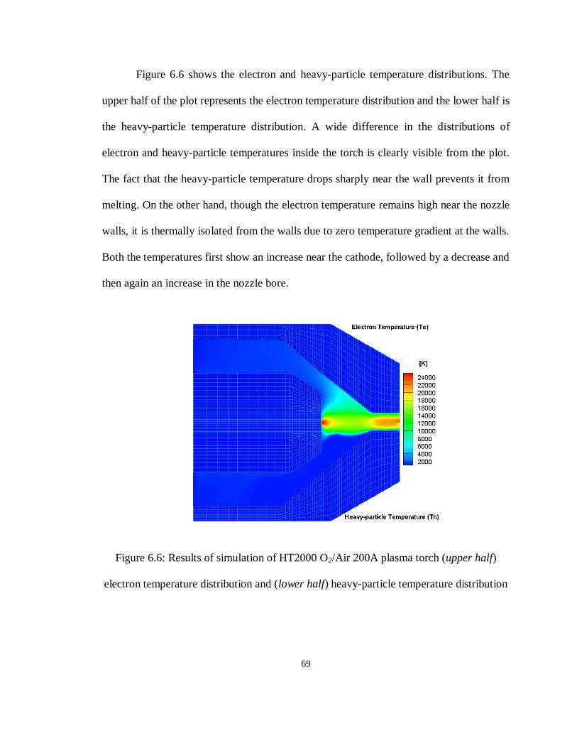
69
Figure 6.6 shows the electron and heavy-particle temperature distributions. The
upper half of the plot represents the electron temperature distribution and the lower half is
the heavy-particle temperature distribution. A wide difference in the distributions of
electron and heavy-particle temperatures inside the torch is clearly visible from the plot.
The fact that the heavy-particle temperature drops sharply near the wall prevents it from
melting. On the other hand, though the electron temperature remains high near the nozzle
walls, it is thermally isolated from the walls due to zero temperature gradient at the walls.
Both the temperatures first show an increase near the cathode, followed by a decrease and
then again an increase in the nozzle bore.
Figure 6.6: Results of simulation of HT2000 O2/Air 200A plasma torch (upper half)
electron temperature distribution and (lower half) heavy-particle temperature distribution

70
The maximum temperatures of ~ 24000 K inside the torch compare with the
maximum temperatures of ~ 28000 K presented in the simulation results by Ghorui et al.
The fact that the new radiation data is almost an order of magnitude greater than the data
used in the earlier simulations seems to have a major effect on the predicted temperature
surrounding the plasma column, which enhances the constriction of the plasma flow. The
larger values of the new volumetric radiation losses predict a stronger radiative cooling of
the arc than what was previously predicted. The stronger cooling of the arc causes the
constriction of the arc observed above (Figure 6.6) and also limits the values of the
temperatures inside the torch.
Figure 6.7 shows the temperature profile at the nozzle exit for the HT 2000 torch.
As expected, the highest temperatures are obtained on the torch axis.
Figure 6.7: Temperature profile at the nozzle exit in HT2000 torch

71
The velocity distribution in the torch is shown in Figure 6.8. The streaks in the
velocity plot are due to the uneven nature of the grid and could be eliminated with the
refinement of the grid as demonstrated in the following sections of this chapter.
Figure 6.8: Velocity distributions in HT2000 torch
The axial velocity profile plot at the nozzle exit shown in Figure 6.9 gives
emphasis on the unphysical off-axis peaks due to the uneven grid.
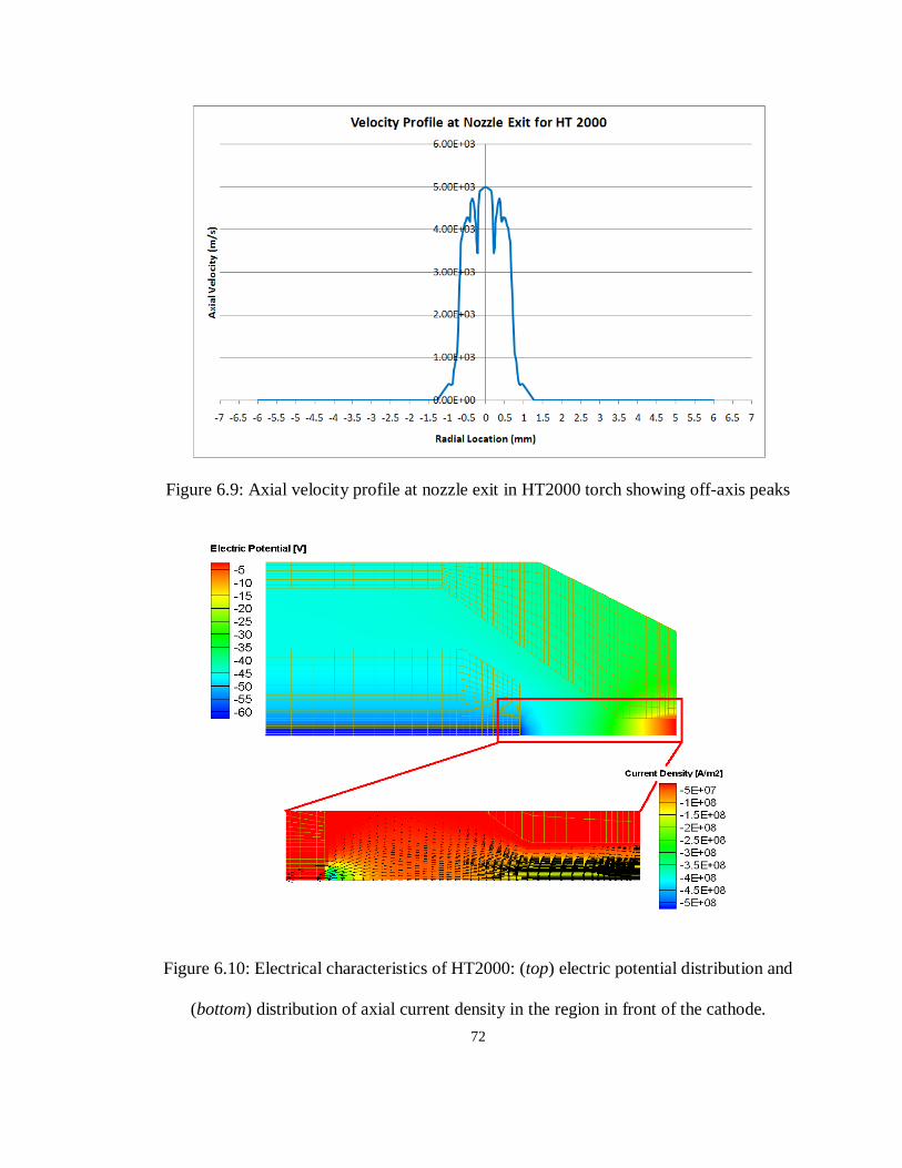
72
Figure 6.9: Axial velocity profile at nozzle exit in HT2000 torch showing off-axis peaks
Figure 6.10: Electrical characteristics of HT2000: (top) electric potential distribution and
(bottom) distribution of axial current density in the region in front of the cathode.

73
Figure 6.10 presents the distribution of electric potential and current density in the
axial direction in the region in front of the cathode. The computational total voltage drop
of ~ 65 V is comparable to the voltage drop obtained experimentally (equal to ~ 63 V).
In the vector plot of the current density as shown in Figure 6.10, the current
distribution is constricted by the cold gas boundary layer along the wall, with the
maximum constriction near the upstream end of the nozzle bore. As the current density
obeys the conservation of current, the highest density is observed in this region as
compared to the region near the cathode where the arc can find more space to expand.
The heat generation mechanism of a plasma torch is by Joule heating. Hence, the
temperature distribution follows the current density distribution.
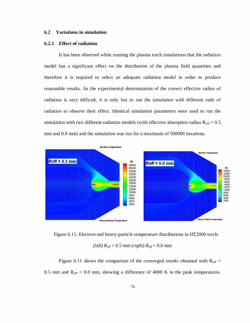
74
6.2 Variations in simulation
6.2.1 Effect of radiation
It has been observed while running the plasma torch simulations that the radiation
model has a significant effect on the distribution of the plasma field quantities and
therefore it is required to select an adequate radiation model in order to produce
reasonable results. As the experimental determination of the correct effective radius of
radiation is very difficult, it is only fair to run the simulation with different radii of
radiation to observe their effect. Identical simulation parameters were used to run the
simulation with two different radiation models (with effective absorption radius Reff = 0.5
mm and 0.0 mm) and the simulation was run for a maximum of 500000 iterations.
Figure 6.11: Electron and heavy-particle temperature distributions in HT2000 torch:
(left) Reff = 0.5 mm (right) Reff = 0.0 mm
Figure 6.11 shows the comparison of the converged results obtained with Reff =
0.5 mm and Reff = 0.0 mm, showing a difference of 4000 K in the peak temperatures.
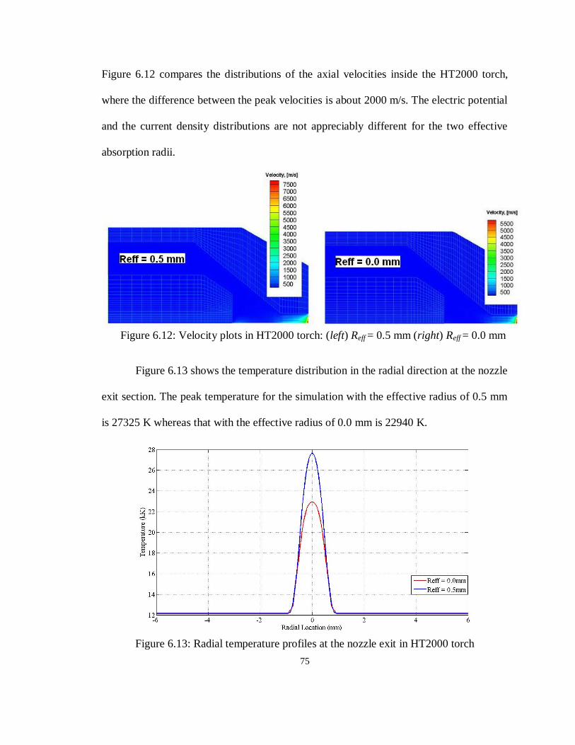
75
Figure 6.12 compares the distributions of the axial velocities inside the HT2000 torch,
where the difference between the peak velocities is about 2000 m/s. The electric potential
and the current density distributions are not appreciably different for the two effective
absorption radii.
Figure 6.12: Velocity plots in HT2000 torch: (left) Reff = 0.5 mm (right) Reff = 0.0 mm
Figure 6.13 shows the temperature distribution in the radial direction at the nozzle
exit section. The peak temperature for the simulation with the effective radius of 0.5 mm
is 27325 K whereas that with the effective radius of 0.0 mm is 22940 K.
Figure 6.13: Radial temperature profiles at the nozzle exit in HT2000 torch

76
The studies performed indicate that the nozzle exit peak temperatures in case of
Reff = 0.0 mm are 2000 K lower than the experimentally measured ones, whereas those in
case of the larger Reff are 2000 K higher.
6.2.2 Solution for off-axis velocity peaks
Figure 6.14: Elimination of off-axis peaks by grid refining

77
As discussed earlier in this chapter the off-axis peaks in the near-exit velocity
profiles are coupled with smoothness of the grid and can be eliminated by adjusting the
grid which is performed as above in Figure 6.14. The grid density distribution in the first
part of the figure is considerably uneven. As the results of NEQ code are highly grid
dependent, this unevenness causes the velocity profile show off-axis peaks at the
locations of abrupt grid density changes. The second part of Figure 6.14 shows a grid
with better density transition as compared to the grid shown in the first part. Therefore, it
results into less prominent off-axis peaks. The third grid shown in Figure 6.14 gives the
best results by almost eliminating the off-axis peaks. The results with this grid are the
closest to the results obtained by Ghorui et al.
6.2.3 Swirl velocity boundary condition correction
The plot of swirl velocity for the HT2000 torch given in Figure 6.15 showed
unrealistically high swirl velocities. The expected value of the swirl velocity at any
location would be in a much lower range as compared to the highest of 900 m/s
(magnitude wise) obtained in the distribution plot.
As evident from the plot, the highest values of swirl velocities are near the inlet
zone which makes one suspect the correctness of the inlet boundary conditions for the
swirl velocity. The following flaw was noticed in the boundary condition subroutine
(BOUNDS.f).

78
Figure 6.15: Swirl velocity w m/s in HT2000 torch
The code solves w.r momentum equation for the swirl velocity w. It was observed
that the value of win (inlet swirl velocity) was given as a boundary condition at the inlet
for w.r equation which is not correct. Figure 6.16 shows the part of BOUNDS.f
subroutine where the above mentioned boundary condition is specified. The expression
inside the highlighted box shows that the value of inlet swirl velocity is assigned as the
boundary condition for the w.r momentum equation.
Figure 6.16: Incorrect w.r inlet boundary condition
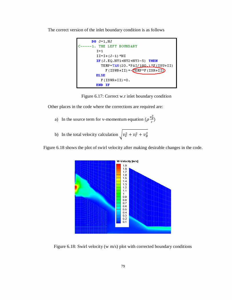
79
The correct version of the inlet boundary condition is as follows
Figure 6.17: Correct w.r inlet boundary condition
Other places in the code where the corrections are required are:
a) In the source term for v-momentum equation
b) In the total velocity calculation
Figure 6.18 shows the plot of swirl velocity after making desirable changes in the code.
Figure 6.18: Swirl velocity (w m/s) plot with corrected boundary conditions
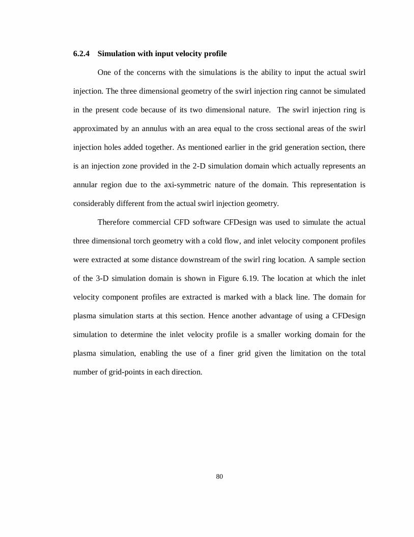
80
6.2.4 Simulation with input velocity profile
One of the concerns with the simulations is the ability to input the actual swirl
injection. The three dimensional geometry of the swirl injection ring cannot be simulated
in the present code because of its two dimensional nature. The swirl injection ring is
approximated by an annulus with an area equal to the cross sectional areas of the swirl
injection holes added together. As mentioned earlier in the grid generation section, there
is an injection zone provided in the 2-D simulation domain which actually represents an
annular region due to the axi-symmetric nature of the domain. This representation is
considerably different from the actual swirl injection geometry.
Therefore commercial CFD software CFDesign was used to simulate the actual
three dimensional torch geometry with a cold flow, and inlet velocity component profiles
were extracted at some distance downstream of the swirl ring location. A sample section
of the 3-D simulation domain is shown in Figure 6.19. The location at which the inlet
velocity component profiles are extracted is marked with a black line. The domain for
plasma simulation starts at this section. Hence another advantage of using a CFDesign
simulation to determine the inlet velocity profile is a smaller working domain for the
plasma simulation, enabling the use of a finer grid given the limitation on the total
number of grid-points in each direction.

81
Figure 6.19: A sample section of torch from CFDesign simulation
Figure 6.20:Comparison of grids for original simulation and simulation with inlet
velocity profile
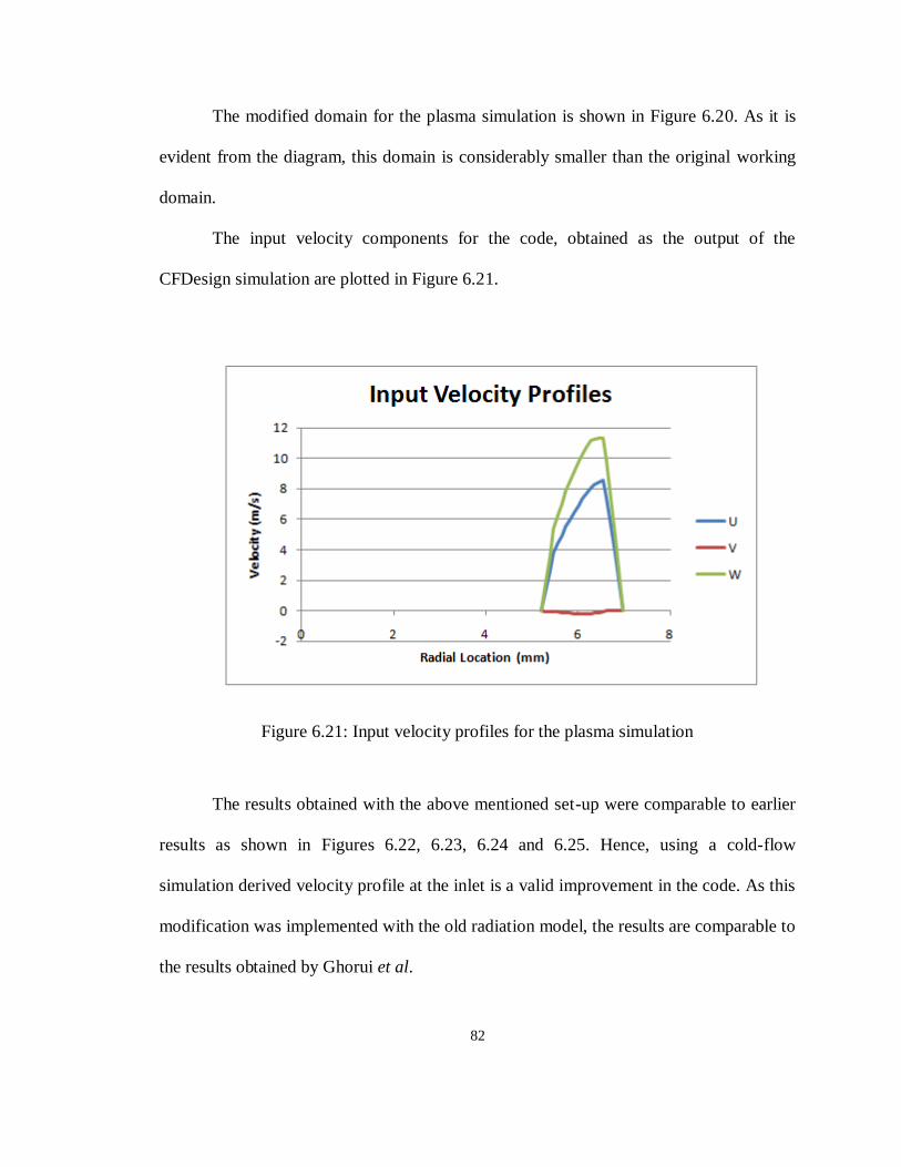
82
The modified domain for the plasma simulation is shown in Figure 6.20. As it is
evident from the diagram, this domain is considerably smaller than the original working
domain.
The input velocity components for the code, obtained as the output of the
CFDesign simulation are plotted in Figure 6.21.
Figure 6.21: Input velocity profiles for the plasma simulation
The results obtained with the above mentioned set-up were comparable to earlier
results as shown in Figures 6.22, 6.23, 6.24 and 6.25. Hence, using a cold-flow
simulation derived velocity profile at the inlet is a valid improvement in the code. As this
modification was implemented with the old radiation model, the results are comparable to
the results obtained by Ghorui et al.
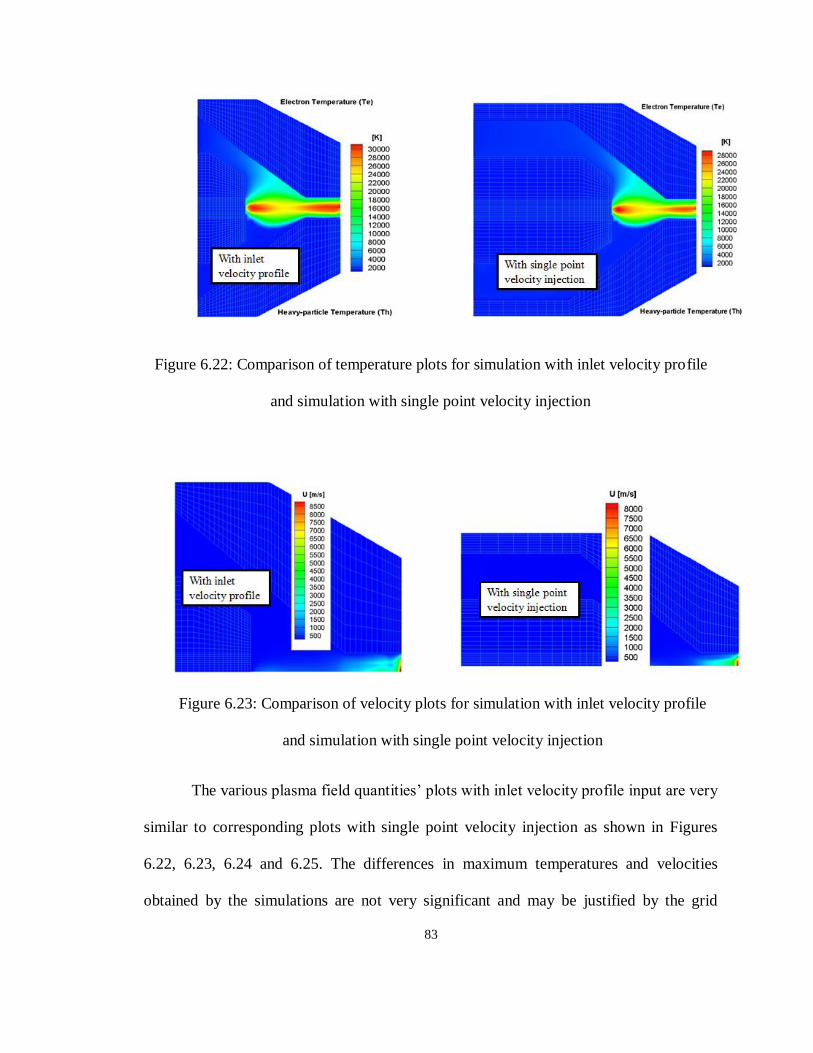
83
Figure 6.22: Comparison of temperature plots for simulation with inlet velocity profile
and simulation with single point velocity injection
Figure 6.23: Comparison of velocity plots for simulation with inlet velocity profile
and simulation with single point velocity injection
The various plasma field quantities‟ plots with inlet velocity profile input are very
similar to corresponding plots with single point velocity injection as shown in Figures
6.22, 6.23, 6.24 and 6.25. The differences in maximum temperatures and velocities
obtained by the simulations are not very significant and may be justified by the grid

84
sensitivity of the code. The grids for the two simulations are significantly different. The
simulation domain for the input velocity profile case is much smaller as compared to the
one for the other case in consideration. Also, the variation might have been introduced by
the software CFDesign used for cold flow simulation.
Figure 6.24: Comparison of axial current density plots for simulation with inlet
velocity profile and simulation with single point velocity injection
Figure 6.25: Comparison of electric potential plots for simulation with inlet velocity
profile and simulation with single point velocity injection

85
6.2.5 Te / Th ratio issue
The degree of non-equilibrium in a plasma torch simulation is quantified by the
ratio of the electron temperature to the heavy-particle temperature. This degree of non-
equilibrium also plays an important role in determining the thermodynamic and transport
properties of the plasma. The present version of the code has properties for the oxygen
plasma with the degree of non-equilibrium up to beyond which the properties get
clipped as shown in Figure 6.26.
Figure 6.26: Augmentation of properties beyond Te / Th = 20 and Te = 45000
(Ghorui, Heberlein, & Pfender, 2006)
The maximum Te / Th ratios as obtained from the simulation are much higher
than 20. Near the nozzle walls, the degree of non-equilibrium is very high due to much
colder heavy particles as compared to those in plasma plume. This is shown in Figure
6.27.

86
Figure 6.27: Plot of Te / Th for HT2000 torch
Excessively high values of Te / Th result in incorrect density values in the region
in the proximity of the nozzle wall as shown in Figure 6.28. The majority of the mass
flow is in this low temperature zone. Hence it is essential to obtain the correct density
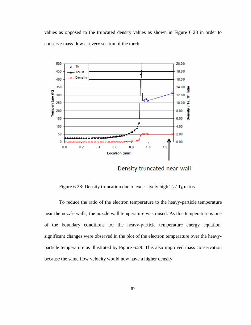
87
values as opposed to the truncated density values as shown in Figure 6.28 in order to
conserve mass flow at every section of the torch.
Figure 6.28: Density truncation due to excessively high Te / Th ratios
To reduce the ratio of the electron temperature to the heavy-particle temperature
near the nozzle walls, the nozzle wall temperature was raised. As this temperature is one
of the boundary conditions for the heavy-particle temperature energy equation,
significant changes were observed in the plot of the electron temperature over the heavy-
particle temperature as illustrated by Figure 6.29. This also improved mass conservation
because the same flow velocity would now have a higher density.

88
Figure 6.29: Corrected values of Te / Th ratios near nozzle wall

89
6.2.6 Second order exit boundary condition
The exit boundary conditions used for the simulation essentially assume a fully
developed flow of plasma. This approach is valid only when the exit conditions are given
at a sufficient distance away from the domain of interest. A better approach for any CFD
simulation would be to use the second order boundary conditions at the exit, as the flow
might not be fully developed in reality in order to use the first order boundary conditions.
The earlier set of exit boundary conditions used and the corresponding new
boundary conditions are illustrated in Table 6.3.
Table 6.3: Earlier and current torch exit boundary conditions

90
The modified boundary conditions were converted into the discretized form with
a finite difference approach for any variable ξ from Table 6.3 as described below.
It was observed that the results were not changed with the modified boundary
conditions. Hence, it is valid to assume a fully developed flow at the exit.

91
6.2.7 Issue with torch exit condition
Figure 6.30: Axial velocity u (m/s) along the torch centerline
Figure 6.30 shows the plot of axial velocity u (m/s) along the torch centerline. As
expected, the velocity increases rapidly in the nozzle portion of the torch but there is a
sudden jump in the velocity near the torch exit, indicating the inaccuracy in representing
the physical conditions at this location.
This problem could be solved with the simulation of the outside-nozzle-exit zone
as this would allow the capturing of the shockwave as the plasma jet ejects out of the
nozzle. This will be a part of the future developments in the code.
0.00E+00
2.00E+03
4.00E+03
6.00E+03
8.00E+03
1.00E+04
1.20E+04
1.20E+01 1.40E+01 1.60E+01 1.80E+01 2.00E+01 2.20E+01
U-final
U-final

92
6.3 Simulation of HT4400 400A O2/Air torch
6.3.1 About the torch (www.hypertherm.com, 2009)
The HySpeed HT4400 is a 400A dry oxygen plasma cutting system. Its single
power supply delivers very high cut speeds – especially on thicker metals. At the same
time, the HT4400 produces virtually no dross and delivers superior cut-face weldability
over the widest range of material types and thicknesses.
Figure 6.31: Cool-core electrode in HT4400
Two proprietary Hypertherm technologies allow high-speed cutting with
maximum consumable life. The LongLife oxygen process involves precise control of key
cutting parameters to gradually ramp up when starting the cut and ramp down when
stopping. These are the times when consumable deterioration is most prevalent. As a
result, the LongLife process significantly extends consumable life.
CoolCore electrodes are designed with the hafnium insert cored-out rather than
utilizing a solid element. This permits heat-extracting copper to be in contact with both

93
the inside and outside surfaces of the hafnium. Transferring heat away from the hafnium
results in a 2-fold increase in electrode life. Because of the cool-core electrode in
HT4400 torch it would be most realistic to use a current density profile which is flat at
the center. This is because of lower centerline temperatures on cathode surface resulting
in lower current density values in accordance with the Richardson-Dushman equation.
A section of HT4400 torch along its axis is shown in Figures 6.32 and 6.33. The
dimensions and other parameters for the grid generation are obtained on the basis of this
drawing.
Figure 6.32: Section of HT4400 with radial dimensions (in mm)

94
Figure 6.33: Section of HT4400 with axial dimensions (in mm)
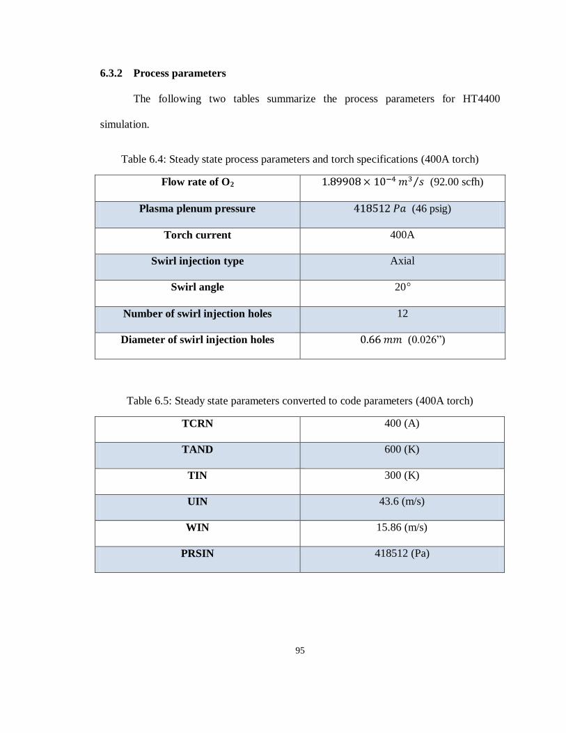
95
6.3.2 Process parameters
The following two tables summarize the process parameters for HT4400
simulation.
Table 6.4: Steady state process parameters and torch specifications (400A torch)
Flow rate of O2 (92.00 scfh)
Plasma plenum pressure (46 psig)
Torch current 400A
Swirl injection type Axial
Swirl angle 20
Number of swirl injection holes 12
Diameter of swirl injection holes (0.026”)
Table 6.5: Steady state parameters converted to code parameters (400A torch)
TCRN 400 (A)
TAND 600 (K)
TIN 300 (K)
UIN 43.6 (m/s)
WIN 15.86 (m/s)
PRSIN 418512 (Pa)

96
6.3.3 Input velocity calculations from inlet flow rate
The calculations follow the steps described in section 6.1.3.
Converting standard flow rate for inlet conditions:
Area of inlet:
Dimensions of inlet zone:

97
6.3.4 Generated grid and simulation results:
The grid generated by the modified grid generator is shown in Figure 6.34.
Figure 6.34: Mesh for HT4400 torch
Figure 6.35 shows the electron and the heavy-particle temperature distributions
for the HT4400 torch for two effective radii of radiation (Reff = 0.0 mm (optically thin
plasma assumption) and Reff = 0.5 mm). The upper half part of the plot represents the
electron temperature distribution and the lower half part is the heavy-particle temperature
distribution. As it is clear from the plots, the model with Reff = 0.5 mm under-predicts the
radiation losses and hence gives unreasonably high temperatures which do not occur in
reality. The current density boundary condition at cathode, used for this simulation is
given by

98
Figure 6.36 shows the velocity distributions for the two effective radii of radiation
(Reff = 0.0 mm (optically thin plasma assumption) and Reff = 0.5 mm). The higher
temperatures obtained with Reff = 0.5 mm in turn lead to higher velocities as compared to
the optically thin model, owing to the more energetic electrons in the former case.
Figure 6.35: Electron and heavy-particle temperature distributions in HT4400
torch: (left) Reff = 0.5 mm (right) Reff = 0.0 mm
Figure 6.36: Velocity distributions in HT4400 torch: (left) Reff = 0.5 mm (right) Reff = 0.0
mm

99
The electric potential and current density plots are shown in Figures 6.37 and
6.38. The potential difference in case of the optically thin model is larger as compared to
the model with Reff = 0.5 mm by about 30 V. This is because of the conservation of the
total energy in spite of the higher energy dissipation in case of the optically thin model.
As the torch current remains 400A and the energy loss due to radiation assumes a higher
value for Reff = 0.0 mm, the potential difference increases in order to conserve the total
energy.
Figure 6.37: Electrical characteristics of HT4400 torch with Reff = 0.5 mm: (top) electric
potential distribution (bottom) axial current density distribution in front of cathode

100
Figure 6.38: Electrical characteristics of HT4400 torch with Reff = 0.0 mm: (top) electric
potential distribution (bottom) axial current density distribution in front of cathode
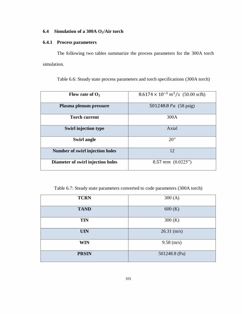
101
6.4 Simulation of a 300A O2/Air torch
6.4.1 Process parameters
The following two tables summarize the process parameters for the 300A torch
simulation.
Table 6.6: Steady state process parameters and torch specifications (300A torch)
Flow rate of O2 (50.00 scfh)
Plasma plenum pressure (58 psig)
Torch current 300A
Swirl injection type Axial
Swirl angle 20
Number of swirl injection holes 12
Diameter of swirl injection holes (0.0225”)
Table 6.7: Steady state parameters converted to code parameters (300A torch)
TCRN 300 (A)
TAND 600 (K)
TIN 300 (K)
UIN 26.31 (m/s)
WIN 9.58 (m/s)
PRSIN 501248.8 (Pa)

102
6.4.2 Input velocity calculations from inlet flow rate
The calculations follow the steps described in section 6.1.3.
Converting standard flow rate for inlet conditions:
Area of inlet:
Dimensions of inlet zone:

103
6.4.3 Generated grid and simulation results:
The grid generated by the modified grid generator is shown in Figure 6.39.
Figure 6.39: Mesh for 300A torch
Figure 6.40 shows the electron and the heavy-particle temperature distributions
for the effective radius of radiation Reff = 0.0 mm (optically thin plasma assumption). The
upper half part of the plot represents the electron temperature distribution and the lower
half part is the heavy-particle temperature distribution. The current density boundary
condition at cathode, used for this simulation is the same as the one used for HT2000 and
HT4400 torches and is given by

104
Figure 6.40: Electron and heavy-particle temperature distributions in 300A torch
with optically thin radiation model
Figure 6.41 presenting the velocity distribution shows a maximum velocity of ~
6000 m/s which is an intermediate value between the maximum values for the 200A (~
5500 m/s) and 400A (~ 6500 m/s) torches.
Figure 6.41: Velocity distributions in 300A torch with optically thin radiation
model

105
Figure 6.42: Electrical characteristics of 300A torch with optically thin model: (left)
electric potential distribution (right) distribution of current density
Figure 6.42 presents the distribution of the electric potential as well as the current
density in the axial direction. The obtained total voltage drop of ~ 75 V is comparable to
the voltage drop of 72 V obtained experimentally.
Figure 6.43 presents a comparison of the nozzle exit temperature profiles for the
three torches in consideration. As expected, the temperatures are in ascending order as we
go from the lowest current value of 200A to the highest current value of 400A. However,
the profiles for the 200A and 300A torches are closer together as compared to the profiles
for the 300A and 400A torches. This is because the HT4400 400A torch has a longer
nozzle bore as opposed to the shorter ones in the other two torches. It is also reflected in
Figure 6.44 showing a comparison of the nozzle exit velocity profiles. As the plasma gas
achieves higher temperatures in the HT4400 torch, we have lower densities for a high
mass flow rate (92 scfh) which results in significantly higher velocity values. Hence we
have higher velocity difference between the 400A and the 300A torch as compared to the
difference between the velocities in the 300A and the 200A torch.
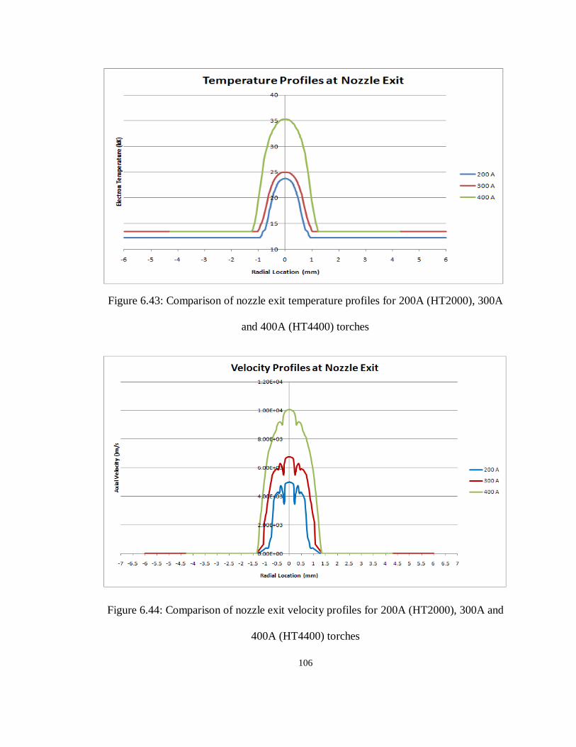
106
Figure 6.43: Comparison of nozzle exit temperature profiles for 200A (HT2000), 300A
and 400A (HT4400) torches
Figure 6.44: Comparison of nozzle exit velocity profiles for 200A (HT2000), 300A and
400A (HT4400) torches

107
7. CONCLUDING REMARKS AND RECOMMENDATIONS
7.1 Concluding remarks
1. A new geometry subroutine (MAKEGRIDX.f) was developed with the ability to
input the nozzle exit cone/counter-bore, vent flow and the specific size and location
of the swirl injection. This routine allowed the complete specification of the
geometrical characteristics (possible in 2-D geometry) of the existing 200A, 300A
and 400A cutting torches from Hypertherm, as well as the future torch designs. The
new routine is recognized by its modularity and user-friendliness. This would make
its further modification, in order to accommodate future design changes,
straightforward.
2. The radiation data for oxygen used in the earlier version of the code underestimated
the radiation losses for the temperatures above ~ 25000 K. New radiation data for
oxygen plasmas, based on the net emission approximation and provided by Gleizes et
al, was incorporated into the NEQ version of FAST-2D.
3. From the simulation of HT2000 with two different effective absorption radii, it was
observed that the radiation loss term had a noticeable effect on the predicted
maximum temperatures and velocities, and only a mild effect on the electrical
characteristics of the flow inside cutting torches. Simulations of the HT2000 torch
using two values of the net absorption radius in the net emission approximation
highlighted the importance of the adequate modeling of the radiative energy transfer
in thermal plasma flow simulations.
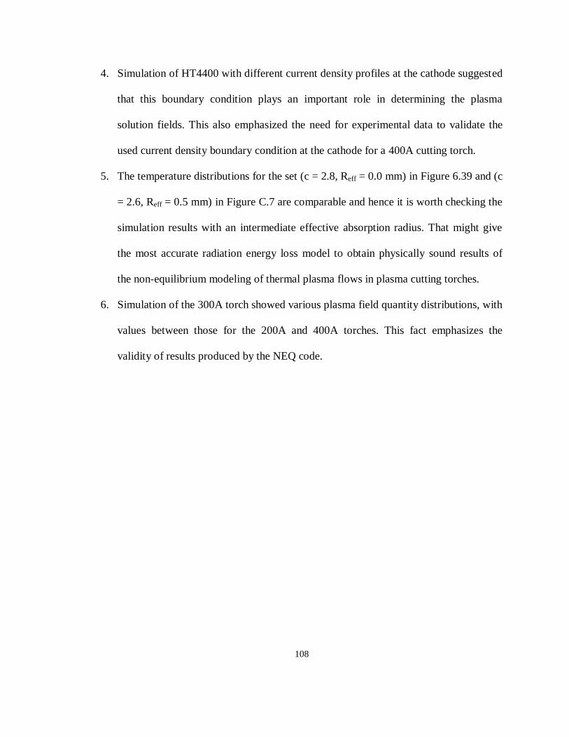
108
4. Simulation of HT4400 with different current density profiles at the cathode suggested
that this boundary condition plays an important role in determining the plasma
solution fields. This also emphasized the need for experimental data to validate the
used current density boundary condition at the cathode for a 400A cutting torch.
5. The temperature distributions for the set (c = 2.8, Reff = 0.0 mm) in Figure 6.39 and (c
= 2.6, Reff = 0.5 mm) in Figure C.7 are comparable and hence it is worth checking the
simulation results with an intermediate effective absorption radius. That might give
the most accurate radiation energy loss model to obtain physically sound results of
the non-equilibrium modeling of thermal plasma flows in plasma cutting torches.
6. Simulation of the 300A torch showed various plasma field quantity distributions, with
values between those for the 200A and 400A torches. This fact emphasizes the
validity of results produced by the NEQ code.

109
7.2 Recommendations
1. Validate the results for the 300A and 400A torches with supporting experimental
work (Electrode temperature measurement for current density boundary condition
and/or spectroscopic measurement of plasma properties at the torch exit).
2. Modify the solver of the code to handle two directional flows (the current version of
the code can handle mainly axial flows but not vent flows and radial swirl injection
geometries).
3. Fix the property code to address very large values of Te / Th ratios - expand tables or
use ideal gas law.
4. Expand model to include cathode boundary condition model by calculated heat flux
to the hafnium from the plasma and heat flux away from hafnium trough conduction.

110
8. BIBLIOGRAPHY
(2009). Retrieved from www.hypertherm.com.
Boulos, M. I., Fauchais, P., & Pfender, E. (1994). Thermal Plasmas: Fundamentals and
Applications. New York: Plenum Press.
Colombo, V., Concetti, A., Ghedini, E., Dallavalle, S., & Vancini, M. (2008). Understanding
Plasma Fluid Dynamics Inside Plasma Torches Through Advanced Modeling. Plasma Science,
IEEE Transactions on 36 , 389-402.
Colombo, V., Ghedini, E., & Mostaghimi, J. (2008). Three-Dimensional Modeling of an
Inductively Coupled Plasma Torch for Spectroscopic Analysis. Plasma Science, IEEE
Transactions on 36 , 1040-1041.
Couch Jr., R. W., Sanders, N. A., Luo, L., Sobr, J., & Backander, P. (1994). Patent No. 5317126.
USA.
Freton, P., Gonzalez, J. J., Gleizes, A., Peyret, F. C., Caillibotte, G., & Delzenne, M. (2002).
Numerical and experimental study of a plasma cutting torch. J. Phys. D: Appl. Phys. 35 , 115-
131.
Freton, P., Gonzalez, J. J., Peyret, F. C., & Gleizes, A. (2006). Complementary experimental and
theoretical approaches to the determination of the plasma characteristics in a cutting plasma torch.
J. Phys. D: Appl. Phys. 36 , 1269-1283.
Ghorui, S., Heberlein, J. V., & Pfender, E. (2006). Hypertherm Report No. 7: Non-Equilibrium
Modeling of Oxygen Plasma - Determination of Non-equilibrium Thermodynamic and Transport
Properties up to 50,000K. University of Minnesota.
Ghorui, S., Heberlein, J. V., & Pfender, E. (2007). Hypertherm Report No. 8: Non-Equilibrium
Modeling of Oxygen Plasma - Determination of Temperature Distribution Using One
Dimensional Arc Model and Development of a General Finite Volume 2-D Grid Generator For
Arc Torches. University of Minnesota.
Ghorui, S., Heberlein, J. V., & Pfender, E. (2006). Hypertherm Report No. 9: Thermodynamic
and transport properties of Two-Temperature Nitrogen-Oxygen plasma. University of Minnesota.
Ghorui, S., Heberlein, J. V., & Pfender, E. (2007). Non-equilibrium modelling of an oxygen-
plasma cutting torch. J. Phys. D: Appl. Phys.40 , 1966-1976.
Ghorui, S., Heberlein, J. V., & Pfender, E. (2007). Thermodynamic and Transport Properties of
Two-temperature Oxygen Plasmas. Plasma Chemistry and Plasma Processing 27 , 267-291.
Gleizes, A., & Cressault, Y. (2007, November). Private Communication. LAPLACE - Université
Paul Sabatier, France.

111
Hsu, K. C., & Pfender, E. (1983). Analysis of the cathode region of a free-burning high intensity
argon arc. J. Phys. D: Appl. Phys. 54 , 3818-3824.
Krey, R. U., & Morris, J. C. (1970). Experimental Total and Total Line Radiation of Nitrogen,
Oxygen, and Argon Plasmas. The Physics of Fluids 13 , 1483.
Li, H. P., & Chen, X. (2001). Diffusion in Two-Temperature Partially Ionized Gases. Chinese
Physics Letters, 18 , 547-549.
Li, H. P., Heberlein, J. V., & Pfender, E. (2004). Hypertherm Report No. 1: Modeling of
Hypertherm Plasma Cutting Torch (HT2000) – Phase 1: Calculation of the Composition and of
Thermodynamic Properties of Two-Temperature Oxygen Plasmas. University of Minnesota.
Li, H. P., Heberlein, J. V., & Pfender, E. (2004). Hypertherm Report No. 2: Modeling of
Hypertherm Plasma Cutting Torch (HT2000) – Phase 2: Basic Equations for the Calculation of
Transport Properties of Two-Temperature Oxygen Plasmas. University of Minnesota.
Li, H. P., Heberlein, J. V., & Pfender, E. (2004). Hypertherm Report No. 3: Modeling of
Hypertherm Plasma Cutting Torch (HT2000) –Phase 3: Composition, Thermodynamic, and
Transport Properties of Two-Temperature Oxygen Plasmas. University of Minnesota.
Li, H. P., Heberlein, J. V., & Pfender, E. (2004). Hypertherm Report No. 4: Modeling of
Hypertherm Plasma Cutting Torch (HT2000) – Phase 4: Physical/Mathematical Two-
Temperature Model. University of Minnesota.
Li, H. P., Heberlein, J. V., & Pfender, E. (2005). Hypertherm report No. 5: Modeling of
Hypertherm Plasma Cutting Torch (HT2000) – Phase 5: A Unified Method for Computing
Incompressible and/or Compressible Flows with Arbitrary Boundaries. University of Minnesota.
Li, H. P., Heberlein, J. V., & Pfender, E. (2005). Hypertherm Report No. 6: Modeling of
Hypertherm Plasma Cutting Torch (HT2000) – Phase 6: Physical/Mathematical Models and
Modeling Results. University of Minnesota.
Lowke, J. J. (1974). Predicitons of Temperature Profiles Using Approximate Emission
Coefficients for Radiation Losses. Journal of Quantitative Spectroscopy Radiative Transfer 14 ,
111-122.
Mitchner, M., & Kruger, C. H. (1992). Partially Ionized Gases. USA: John Wiley & Sons, Inc.
Nemchinsky, V. A. (1998). Plasma flow in a nozzle during plasma arc cutting. J. Phys. D: Appl.
Phys. 31 , 3102-3107.
Patankar, S. V. (1980). Numerical Heat Transfer and Fluid Flow. New York: McGraw-Hill.
Peters, J. (2003). Cathode erosion in a plasma cutting torch. MS Thesis . University of Minnesota,
MN.

112
Ramakrishnan, S., Gershenzon, M., Polivka, F., Kearney, T. N., & Rogozinsk, M. W. (1997).
Plasma Generation for the Plasma Cutting Process. IEEE TRANSACTIONS ON PLASMA
SCIENCE 25 , 937-946.
Schnick, M., Füssel, U., & Zschetzsche, J. (2006). Simulation of plasma and shielding gas flows
in welding and cutting arcs with Ansys CFX. Modelling for Material Processing. Riga:
International Scientific Colloquium.
Trelles, J. P., Heberlein, J. V., & Pfender, E. (2007). Hypertherm Report No. 1: Modeling of
Hypertherm Plasma Cutting Torches (HT4400 and 9427 Rev1). University of Minnesota.
Trelles, J. P., Heberlein, J. V., & Pfender, E. (2007). Hypertherm Report No. 2: Modeling of
Hypertherm Plasma Cutting Torches (HT4400 and 9427 Rev1). . University of Minnesota.
Vincenti, W. G., & Kruger, C. H. (1965). Introduction to Physical Gas Dynamics. New York:
John Wiley and Sons.
www.castolin.com. (2009).
www.dgkk.de. (2009). Retrieved from http://www.dgkk.de/PDF/kinsim09/Spille_Kohoff.pdf.
Zhou, X., & Heberlein, J. V. (1998). An experimental investigation of factors affecting arc-
cathode erosion. Journal of Physics D: Applied Physics , 2577-2590.
Zhu, J. (1991). FAST-2D: A computer program for numerical simulation of two-dimensional
incompressible flows with complex boundaries. Institute for hydromechanics, University of
Karlsruhe.

113
APPENDIX A: VARIABLES IN FAST-2D
Geometry Variables:
Variable Description Index1
ISCOX, ISCOY x, y coordinates of control volume vertices (grid-corner
points)
1,2
ISX, ISY x, y coordinates of control volume center 3,4
ISR Coordinate r of cylindrical coordinates 5
ISFX, ISFY2 Linear Interpolation factors fx , fy 6,7
ISVOLP Volume of control volume 8
ISB11W ynw – ysw 9
ISB12W xsw – xnw 10
ISB21W yW– yP 11
ISB22W xP – xW 12
ISB11S yP – yS 13
ISB12S xS – xP 14
ISB21S ysw– yse 15
ISB22S xse – xsw 16
ISB11P yn – ys 17
ISB12P xs – xn 18
ISB21P yw – ye 19
ISB22P xe – xw 20
Figure A1 : A typical control volume centered at node P along with neighboring nodes
(Zhu, 1991)

114
Other Variables:
Variable Description Index
ISPP3 Pressure correction 21
ISU Axial velocity at time level n 22
ISV Radial velocity at time level n 23
ISWR (Azimuthal velocity )W.r 24
ISTE Turbulent kinetic energy at time level n 25
ISED Dissipation rate (ε) at time level n 26
ISAH Enthalpy at time level n 27
ISTEM Electron temperature at time level n 28
ISEP Electric potential at time level n 29
ISZFE Species Concentration- Electrons at time
level n
30
ISZFI Species Concentration- Heavy Particles at
time level n
31
ISP Pressure at time level n 32
ISDEN Mass density at time level n 33
ISMUT Turbulent viscosity 34
ISW Azimuthal velocity at time level n 35
ISCW, ISCS Convective coefficients Cw ,Cs 36,37
ISAW, ISAE, ISAS,
ISAN, ISAP
Coefficients AW , AE , AS , AN , AP 38,39,40,41,42
ISSU, ISSP Source terms for difference equation 43,44
ISAPU, ISAPV 1/Ap for U and V momentum equation 45,46
ISSUMU, ISSUMV (AE , AW , AN , AS)/ AP for U and V
momentum equation
47,48
ISP1 Pressure at time level n-1 49
ISU1 Axial velocity at time level n-1 50
ISV1 Radial velocity at time level n-1 51
ISW1 Azimuthal velocity at time level n-1 52
ISK1 Turbulent kinetic energy at time level n-1 53
ISE1 Dissipation rate (ε) at time level n-1 54
ISAH1 Enthalpy at time level n-1 55
ISTEM1 Electron temperature at time level n-1 56
ISEP1 Electric potential at time level n-1 57
ISZFE1 Species Concentration- Electrons at time
level n-1
58
ISZFI1 Species Concentration- Heavy Particles at
time level n-1
59
ISP2 Pressure at time level n-2 60
ISU2 Axial velocity at time level n-2 61

115
ISV2 Radial velocity at time level n-2 62
ISW2 Azimuthal velocity at time level n-2 63
ISK2 Turbulent kinetic energy at time level n-2 64
ISE2 Dissipation rate (ε) at time level n-2 65
ISAH2 Enthalpy at time level n-2 66
ISTEM2 Electron temperature at time level n-2 67
ISEP2 Electric potential at time level n-2 68
ISZFE2 Species Concentration- Electrons at time
level n-2
69
ISZFI2 Species Concentration- Heavy Particles at
time level n-2
70
ISGAM, ISGAMW,
ISGAMS
Effective diffusion coefficient 71, 72, 73
ISB Azimuthal component of self induced
magnetic field
74
ISJX Axial current density component 75
ISJR Radial current density component 76
ISDEN1, ISDEN2 Density at time level n-1, n-2 77, 78
ISUW, ISVW, ISUS,
ISVS
Velocity interpolations on west and south
faces
79, 80, 81, 82
ISTMH,
ISTMH1,ISTMH2
Heavy particle temperature at time levels n,
n-1, n-2
83, 84, 85
1 Index number in represents the order of the corresponding variable in array F 2 Interpolation factors are given by: fx = lwW / (lPw + lwW) & fy = lsS / (lPs + lsS)
where lwW , lwW , lwW , lwW are lengths of linear segments wW, Pw, sS, Ps 3 Variables in red are the ones for which the governing equations are solved
Figure A2 : Layout and indexing of cell center and corner points (Zhu, 1991)

116
APPENDIX B: SUBROUTINES AND OUTPUT FILES IN NEQ CODE
Code Subroutines:
1. BOUNDS: boundary conditions geometry specific
2. COEFF: FAST2D, coefficients
3. FILES_SPEBND: FAST2D, boundary conditions; i.e. for solid domains, specify
4. FLOSOL: FAST2D, solver
5. USER: Inputs from user
6. INTIA_CURRENT: inserts current density profile as a boundary condition
7. SETJ: calculates current density profile
8. MAIN: Calls other subroutines
9. MAKEGRIDX: mesh generation
10. OVACON: checks overall conservation (~ SIMPLEC algorithm)
11. SAVINGS_MAGNET: generation of TECPLOT files
12. SOURCE: specification source terms
Output Files:
Output files are generated each 500 iterations
MESH: complete mesh
TEMxxxx: electron temperature
TMHxxxx: heavy and electron temperature
VELxxxx: velocity
FAIxxxx: potential
CURxxxx: current density
MCHxxxx: Mach number
Here xxxx represents the file number.

117
APPENDIX C: SOLUTION FIELDS FOR A RANGE OF CURRENT
DENSITY PROFILE BOUNDARY CONDITIONS AT THE CATHODE FOR
REFF = 0.5 MM IN HT4400 TORCH
1) →
Figure C.1: Results with : (left) temperature distribution and (right) velocity distribution
Figure C.2: Results with : (left) electric potential distribution and (right) current
density distribution

118
2) →
Figure C.3: Results with : (left) temperature distribution and (right) velocity
distribution
Figure C.4: Results with : (left) electric potential distribution and (right) current
density distribution

119
3) →
Figure C.5: Results with : (left) temperature distribution and (right) velocity
distribution
Figure C.6: Results with : (left) electric potential distribution and (right) current
density distribution

120
4) →
Figure C.7: Results with : (left) temperature distribution and (right) velocity
distribution
Figure C.8: Results with : (left) electric potential distribution and (right) current
density distribution
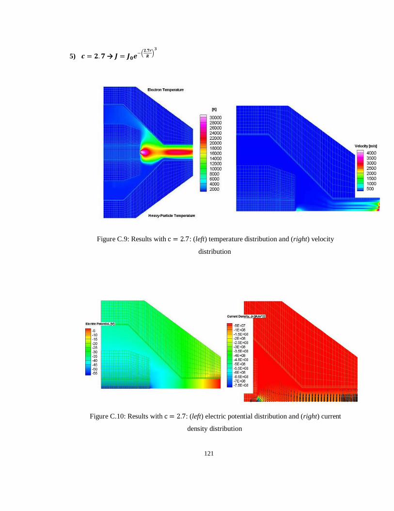
121
5) →
Figure C.9: Results with : (left) temperature distribution and (right) velocity
distribution
Figure C.10: Results with : (left) electric potential distribution and (right) current
density distribution

122
6) →
Figure C.11: Results with : (left) temperature distribution and (right) velocity
distribution
Figure C.12: Results with : (left) electric potential distribution and (right) current
density distribution