Numerical modeling of coupled water flow and heat ... · Numerical Modeling of Coupled Water Flow...

Soil Science Society of America Journal

Soil Sci. Soc. Am. J. 80:247–263 doi:10.2136/sssaj2015.07.0279 Received 3 Aug. 2015. Accepted 9 Dec. 2015. *Corresponding author ([email protected]). © Soil Science Society of America, 5585 Guilford Rd., Madison WI 53711 USA. All Rights reserved.

Numerical Modeling of Coupled Water Flow and Heat Transport in Soil and Snow

Soil Physics & Hydrology

A one-dimensional vertical numerical model for coupled water flow and heat transport in soil and snow was modified to include all three phases of water: vapor, liquid, and ice. The top boundary condition in the model is driven by incoming precipitation and the surface energy balance. The model was applied to three different terrestrial systems: a warm desert bare lysimeter soil in Boulder City, NV; a cool mixed-grass rangeland soil near Laramie, WY; and a snow-dominated mountainous forest soil about 50 km west of Laramie, WY. Comparison of measured and calculated soil water contents with depth yielded modeling efficiency (ME) values (maximum range: −¥ < ME £ 1) of 0.32 £ ME £ 0.75 for the bare soil, 0.05 £ ME £ 0.30 for the rangeland soil, and 0.06 £ ME £ 0.37 for the forest soil. Results for soil temperature with depth were 0.87 £ ME £ 0.91 for the bare soil, 0.92 £ ME £ 0.94 for the rangeland soil, and 0.85 £ ME £ 0.88 for the forest soil. The model described the mass change in the bare soil lysimeter due to outgoing evaporation with moderate accuracy (ME = 0.41, based on 4 yr of data and using weekly evaporation rates). Snow height for the rangeland soil and the forest soil was captured reasonably well (ME = 0.57 for both sites based on 5 yr of data for each site). The model is physics based, with few empirical parameters, making it applicable to a wide range of terrestrial ecosystems.

Abbreviations: LAI, leaf area index; ME, modeling efficiency.

The ability to understand and quantify temporal dynamics in water and heat storage in soil and snow is important across a range of terrestrial eco-systems. The modeling of water and heat fluxes in the soil–plant–atmo-

sphere system is used in many disciplines such as agriculture, structural engineer-ing, hydrology, ecology, and climate science. Increasingly detailed algorithms on water and heat exchange are now also routinely included in watershed- and basin-scale computer simulation models to improve regional water management. The effect of climate change and land use change on modifying water and heat fluxes are a particularly active area of research at present.

Water in soil and snow is stored in three phases: liquid, vapor, and solid (ice). Water flow and heat transport are coupled processes. For example, vaporizing liq-uid water requires heat and freezing liquid water releases heat as the water mol-ecules are moved to a higher and lower energy state, respectively. Soil salinity influ-ences the vaporization and freezing processes by lowering the energy state of the liquid water, reducing vaporization rates, and delaying the onset of freezing. Soil type has a similar effect, with fine-textured soils having higher water retention thus reducing the energy state of the water.

The theory of water flow, heat transport, and phase change in soil and snow has been worked out during the past decades. Philip and de Vries (1957) showed how liquid water and water vapor transfer may be separated into isothermal and thermal components. Guymon and Luthin (1974) used the Clapeyron equation

Thijs J. Kelleners*Dep. of Ecosystem Science and Management Univ. of Wyoming Laramie, WY 82071

Jeremy Koonce Rose Shillito Jelle Dijkema Markus Berli

Division of Hydrologic Sciences Desert Research Institute Las Vegas, NV 89119

Michael H. YoungBureau of Economic Geology Univ. of Texas Austin, TX 78758

John M. Frank W.J. Massman

US Forest Service Rocky Mountain Research Station Fort Collins, CO 80526

Core Ideas

•Models of coupled water flow and heat transport improve our understanding of ecosystems.

•Soil and snow liquid water flow, water vapor flow, and ice are described using numerical models.

•The model is verified for a bare desert soil, a rangeland soil, and a forest soil.

Published April 22, 2016

248 Soil Science Society of America Journal

and the soil water retention curve to relate freezing temperature to liquid water potential and liquid water content in frozen soils. Fuchs et al. (1978) incorporated the effect of osmotic potential into the relationship between freezing temperature and water potential in frozen soil. Nassar and Horton (1989) added osmot-ic effects to the relationship between soil liquid water potential and soil air relative humidity.

The calculation of water flow and heat transport in soil and snow generally requires numerical techniques due to the hetero-geneous nature of the media and the variable boundary condition with the atmosphere. Root water uptake further complicates mat-ters. Early models treated water flow and heat transport separately and neglected vapor and ice. Subsequent models incorporated either water vapor flow (Fayer, 2000; Saito et al., 2006) or freez-ing (Harlan, 1973; Dall’Amico et al., 2011). Relatively few mod-els consider all three phases of water simultaneously (Zhao et al., 1997; Hansson et al., 2004; Painter, 2011). Even fewer models treat water flow and heat transport in soil and snow with the same rigor (Flerchinger and Saxton, 1989; Flerchinger, 2000).

The purpose of this study was to develop a rigorous numeri-cal model for coupled water flow and heat transport in soil and snow. The model is an extension of that presented by Kelleners et al. (2009), Kelleners and Verma (2012), and Kelleners (2013). The earlier versions of the model included only water phase change due to freeze–thaw. The new model now also includes water vapor flow. The canopy and surface energy balance, as ex-plained in the previous studies, remains largely unchanged, in-cluding the ability to calculate incoming solar radiation in com-plex terrain. Within-canopy transfer of sensible and latent heat was modified for this study by using an exponential wind profile as proposed by Dolman (1993). Soil evaporation and root water uptake were modified based on recent studies by Tang and Riley (2013) and de Jong van Lier et al. (2008), respectively. The effect of ion concentration on coupled flow and transport was incorpo-rated by assuming that the solute mass in the soil profile is time invariant, with solute concentration increasing (decreasing) as the soil water content decreases (increases).

The specific objectives of the study were: (i) to develop the coupled water flow and heat transport equations for soil and snow; (ii) to apply the model to a warm-climate bare soil where water vapor flow might be relatively significant; (iii) to apply the model to a cold-climate rangeland soil where soil freezing is significant; and (iv) to apply the model to a cold-climate moun-tainous forest soil where snow accumulation and melt dominate the annual hydrological cycle. With the first case (bare soil con-tained in a lysimeter), the lysimeter weight change was used to verify the calculated water fluxes due to incoming precipitation and outgoing soil evaporation. In addition, calculated water and heat fluxes were validated indirectly by comparing the measured and calculated soil water contents and soil temperatures. For the other two cases, no direct flux measurements were available and the calculated water and heat fluxes were both validated indirectly by determining the model’s ability to replicate the measured soil water contents, soil temperatures, and snow height dynamics.

THEORYThe main water flow and heat transport equations are pro-

vided in this section as well as a description of the updated cal-culation methods for within canopy transfer, soil evaporation, and root water uptake. Expressions for the non-zero derivative terms used are given in the appendix. The coupled water flow and heat transport equations are solved using flexible time step-ping, where the time step is decreased (increased) as the number of iterations needed to solve the equations increases (decreases) following Šimůnek et al. (2013).

Snow Water FlowWater movement in snow is the result of liquid water flow

due to gravity and water vapor flow due to a temperature gradi-ent (Colbeck and Davidson, 1973; Colbeck, 1993; Pinzer et al., 2012):

( )vs a 3w i iws e vT

w w

1 TK S Kt t t z z

r qq r qr r

∂∂ ∂ ∂ ∂ + + = + ∂ ∂ ∂ ∂ ∂ [1]

where qw is liquid water content (m3 m−3), qa is air content (m3 m−3), qi is ice content (m3 m−3), rw is liquid water density (kg m−3), rvs is saturated water vapor density (kg m−3), ri is ice den-sity (kg m−3), t is time (s), Se is relative saturation (dimension-less), Kws is saturated snow hydraulic conductivity (m s−1), KvT is thermal water vapor hydraulic conductivity (m2 s−1 K−1), T is temperature (°C), and z is the vertical coordinate (m). It is as-sumed that snow water vapor is always at saturation (e.g., Oleson et al., 2013). The relative saturation of liquid water in snow is ( Jordan, 1991)

w wre

wr1S q q

q−

=−

[2]

where qwr is the residual liquid water content (m3 m−3) given as (Tarboton and Luce, 1996)

c snwr

w

F rq

r= [3]

where Fc = 0.02 is the mass of liquid water that can be retained per mass of dry snow (kg kg−1), and the snow bulk density rsn (kg m−3) is calculated as

sn w w i ir q r q r= + [4]

The snow hydraulic conductivities are (Shimizu, 1970; Colbeck, 1993)

2w snws gr

w

7.80.077 exp

gK dr rh r

−=

[5a]

vsvT

w

dd

DKTr

r= [5b]

where g is acceleration due to gravity (m s−2), h is liquid water vis-cosity (kg m−1 s−1), dgr is snow grain diameter (m), and D is water vapor diffusivity (m2 s−1). The grain diameter for each snow layer

www.soils.org/publications/sssaj 249

is calculated as a function of snow temperature, snow liquid water content, and snow age (Kelleners et al., 2009). The vapor diffu-sivity in snow is calculated by assuming that vapor movement is unobstructed by ice (or liquid water) and that there is no diffu-sion enhancement, based on experimental data and theoretical considerations presented by Pinzer et al. (2012), so that

aD D= [6]

where Da is the diffusivity of water vapor in bulk air (m2 s−1). Use of qa = 1 − qi − qw, application of the product rule, and rear-rangement of Eq. [1] results in the following mass balance equa-tion:

vs w vs a vsi i

w w w w

3ws e vT

1tt t

TK S Kz z

r q r q rr qr r r r

∂ ∂∂− + − + = ∂ ∂ ∂ ∂ ∂ + ∂ ∂

[7]

The mass balance equation is written in terms of the unknown Se using the chain rule and by noting that dqi/dSe and drvs/dSe are zero:

vs w e vs a vsi i

w e w w w

3ws e vT

d1

d tS

S t tTK S K

z z

r q r q rr qr r r r

∂ ∂∂− + − + = ∂ ∂ ∂ ∂ ∂ + ∂ ∂

[8]

The mass balance equation is solved for Se by using the mixed formulation of Celia et al. (1990) where the three storage terms in Eq. [1] are combined with the single ¶Se/¶t term in Eq. [8] to describe the change in storage with time. The creation, com-paction, and merger of snow layers is handled at each time step outside the numerical solution. Compaction due to metamor-phism and overburden follows Jordan (1991). Snow layers that drop below a preset minimum thickness (1 cm in this study) are merged with an underlying layer. Snow layers that exceed a preset maximum thickness (2 cm in this study) are split into equal parts (Kelleners et al., 2009).

Soil Water FlowWater movement in soil is due to pressure head gradients,

temperature gradients, and gravity (the effect of gravity on water vapor is ignored). The soil water flow equation is (Hansson et al., 2004; Saito et al., 2006)

( )r vs aw i i

w w

wh wh wT

vh vT w

1 Ht t t

h TK K Kz z z

h TK K Sz z

r qq r qr r

∂∂ ∂+ + =

∂ ∂ ∂∂ ∂ ∂ + +∂ ∂ ∂

∂ ∂ + + −∂ ∂

[9]

where Hr is soil air relative humidity (dimensionless), h is soil water pressure head (m), Kwh is isothermal liquid water hydraulic

conductivity (m s−1), KwT is thermal liquid water hydraulic con-ductivity (m2 s−1 K−1), Kvh is isothermal water vapor hydrau-lic conductivity (m s−1), KvT is thermal water vapor hydraulic conductivity (m2 s−1 K−1), and Sw is a sink term for root water uptake (s−1). Assuming that the contributions from the pressure potential and osmotic potential are additive, and the solute is conservative, the relative humidity (as a fraction) is (Nassar and Horton, 1992)

( )w

r ww

exp , 0273.15

hM gH MM hR T

fq

= − ≤ +

[10]

where Mw is the molecular mass of water (kg mol−1), M is mo-lality at saturation (mol kg−1 of solvent), R is the gas constant ( J mol−1 K−1), and f is porosity (m3 m−3). The soil hydraulic conductivities are (Hansson et al., 2004; Saito et al., 2006)

( ) i

21/

wh whs e e1 1 10mmK K S Sl Wq− = − − ×

[11a]

wT wh0

1 dd

K K hGTg

g= [11b]

vs rvh

w

ddHK Dh

rr

= [11c]

vs rvT e r e vs

w w

d dd d

D D HK HT Tr

h h rr r

= + [11d]

where Kwhs is saturated soil liquid water hydraulic conductivity (m s−1), m (dimensionless) and l (dimensionless) are empirical parameters in the van Genuchten–Mualem soil hydraulic func-tions, W is an impedance factor (dimensionless), G = 4 is a gain factor (dimensionless), g is soil water surface tension (kg s−2), g0 is soil water surface tension at 25°C (kg s−2), and he is an en-hancement factor (dimensionless) as derived by Cass et al. (1984). Values for the impedance factor, which describes the blocking of pores due to ice formation (e.g., Hansson et al., 2004), were set to zero for all soil layers, except for the rangeland soil where W = 4.4 was used below the 40-cm depth based on a previous model cali-bration (Kelleners, 2013). The soil relative saturation and water retention function are (van Genuchten, 1980)

( )w wre

wr

1 , 0mnS h hq q

af q

−−= = + ≤

− [12]

where a (m−1) and n (dimensionless) are empirical param-eters, with m = 1 − 1/n. The diffusivity of water vapor in soil is (Moldrup et al., 1999)

1 3/a

a a a a 3/

b

bD D D q

q t qf

+

= = [13]

where t is the tortuosity factor (dimensionless) and b is the Campbell soil water retention parameter (dimensionless) ap-proximated as 1/(n − 1). The use of qa = f − qi − qw, application


of the triple product rule, and rearrangement of Eq. [9] results in the following mass balance equation:

r vs w r vsi i

w w w

vs a r a vsr

w w

wh wh wT

vh vT w

1H H

t tHH

t th TK K K

z z zh TK K Sz z

r q rr qr r r

r q q rr r

∂ ∂− + − ∂ ∂

∂∂+ + =

∂ ∂∂ ∂ ∂ + +∂ ∂ ∂

∂ ∂ + + −∂ ∂

[14]

The mass balance equation is written in terms of the unknown h using the chain rule and by noting that drvs/dh is zero:

r vs w r vsi i

w w w

vs a r a vsr

w w

wh wh wT

vh vT w

d d1

d ddd

H Hh hh t h t

HH hh t t

h TK K Kz z z

h TK K Sz z

r q rr qr r r

r q q rr r

∂ ∂− + − ∂ ∂

∂∂+ + =

∂ ∂∂ ∂ ∂ + +∂ ∂ ∂

∂ ∂ + + −∂ ∂

[15]

The mass balance equation is solved for h by using the mixed for-mulation of Celia et al. (1990), where the three storage terms in Eq. [9] are combined with the three ¶h/¶t terms in Eq. [15] to describe the change in storage with time. Note that dqi/dh = −dqw/dh for saturated frozen soils, while dqi/dh = 0 for unsaturat-ed soils. This avoids the need for a separate water flow equation for saturated frozen conditions, as was used by Kelleners (2013).

Snow–Soil Heat TransportHeat transport is due to conduction and convection and is

calculated using (Hansson et al., 2004; Saito et al., 2006)

( ) ( )r vs a iv f i

w w v w v v w v

w w

HCTt t t

T C q T c q T qz zC S T

r q qg g r

k r g r

∂∂ ∂+ − =

∂ ∂ ∂∂ ∂ − − − ∂ ∂ −

[16]

where C is bulk snow-soil heat capacity ( J m−3 K−1), gv is latent heat of vaporization ( J kg−1), gf is latent heat of fusion ( J kg−1), k is bulk snow–soil thermal conductivity ( J m−1 s−1 K−1), Cw is liquid water heat capacity ( J m−3 K−1), cv is water vapor heat capacity ( J kg−1 K−1), qw is liquid water flux (m s−1), and qv is water vapor flux (expressed as an equivalent liquid water flux, m s−1). Note that Hr = 1 for snow and 0 £ Hr £ 1 for soil. The snow and soil volumetric heat capacities are, respectively,

w w i i a aC C C Cq q q= + + [17a]

( ) s w w i i a a1C C C C Cf q q q= − + + + [17b]

where Ci is heat capacity of ice ( J m−3 K−1), Ca is heat capac-ity of air ( J m−3 K−1), and Cs is heat capacity of solids ( J m−3 K−1). The snow and soil thermal conductivities are, respectively ( Jordan, 1991; Farouki, 1981),

( )( )

5 6 2a sn sn

i a

7.75 10 1.105 10k k r r

k k

− −= + × + ×

× − [18a]

( )dry KN sat dryFk=k + k -k [18b]

where ka is thermal conductivity of air ( J m−1 s−1 K−1), ki is thermal conductivity of ice ( J m−1 s−1 K−1), kdry is thermal con-ductivity of dry soil ( J m−1 s−1 K−1), ksat is thermal conductivity of saturated soil ( J m−1 s−1 K−1), and FKN is the Kersten num-ber (dimensionless). The Kersten number is a function of the degree of saturation and the phase of water (Oleson et al., 2013). Application of the triple product rule and the volume relation-ship dqi = −dqw results in

( ) vsrv vs a v r a

a wv r vs f i

w w v w v v w v

w w

CT H Ht t t

Ht t


rg r q g q

q qg r g r

k r g r

∂ ∂∂+ +

∂ ∂ ∂∂ ∂

+ + =∂ ∂

∂ ∂ − − − ∂ ∂ −

[19]

The energy balance equation is written in terms of the unknown T using the chain rule and by noting that dqa/dT is zero:

( ) vsrv vs a v r a

a wv r vs f i

w w v w v v w v

w w

ddd d

dd

CT H T THt T t T t

THt T t


rg r q g q

q qg r g r

k r g r

∂ ∂ ∂+ +

∂ ∂ ∂∂ ∂

+ + =∂ ∂

∂ ∂ − − − ∂ ∂ −

[20]

The energy balance equation is solved for T by using the mixed formulation of Celia et al. (1990), where the three storage terms in Eq. [16] are combined with the three ¶T/¶t terms in Eq. [20] to describe the change in storage with time. Note that Kelleners (2013) used the mass relationship dqi = −rwdqw/ri instead of the volume relationship dqi = −dqw to eliminate qi from the heat transport equation for unsaturated frozen soils. Both options have been used in the literature (e.g., Fuchs et al., 1978; Hansson et al., 2004). The benefit of using the volume relationship for both unsaturated and saturated frozen soil conditions is that it avoids the need for a separate soil water flow equation for satu-rated frozen conditions. The use of either the volume or mass relationship seems to have little impact on the resulting calcula-tions, based on limited testing. (See Kelleners [2013] for more details on the solution strategy for the coupled water flow and heat transport equations.)


Soil–Plant–Atmosphere TransferThe model calculates the complete

canopy and ground surface energy balance by solving for the canopy and ground surface temperatures, respectively (complete equa-tion set given in Kelleners et al. [2009] and Kelleners and Verma [2012]). Previously, the surface resistance to soil evaporation was ignored and the latent and sensible heat flux between the soil surface and the canopy air was calculated by weighing the trans-fer coefficients of bare ground and shaded ground (e.g., Oleson et al., 2013). For the current study, the conductance factors that govern the exchange of latent and sensible heat in the soil–plant–atmosphere system were updated in two significant ways: First, soil evaporation is now regulated by con-ductance factors for liquid water flow and water vapor flow (acting in parallel) in the upper half of the top soil element to describe surface resistance. Second, the transfer of water vapor and heat in the canopy air space is now calculated by assuming an exponen-tial wind profile within the canopy. Above-canopy transfer continues to be based on a logarithmic wind profile. The conductance factors are depicted in Fig. 1 for vegetated and unvegetated sur-faces. Soil water vapor flow conductance Gv (m s−1) and soil liquid water flow conductance Gw (m s−1) are calculated following Tang and Riley (2013):

v1

2Dz

GD

= [21a]

( )wh w ww

1 r vs

2 d dK hz H

q rG

D r= [21b]

where Dz1 is thickness of the top soil element (m). A downside of these soil conductance factors is their dependence on the spatial discretization of the surface (the Dz1 term). This implies that the calculated latent heat flux will be influenced in part by the top soil element thickness. This effect is at least partly offset by the fact that the diffusion terms D and Kwhdh/dqw for the topsoil can be expected to increase (decrease) as Dz1 increases (decreases) in a drying soil, thus partly compensating for the Dz1 dependency. The conductance factors for canopy air transfer Gca,u (lower can-opy, m s−1) and Gca,a (higher canopy, m s−1) are calculated using an exponential wind profile following Dolman (1993):

( )

vege e,ca,u

e veg

1

e 0g e 0 v

veg veg

exp( )

exp exp

zn D

n z

n z n d zz z

G

−

=

− − + × −

[22a]

veg

1

e e, 0 vca,a e

veg veg

exp 1 1zn D d zn

z zG

− + = − −

[22b]

where ne is a dimensionless eddy decay coefficient (3.0 for grass and 6.0 for coniferous forest in this study), De,zveg is an eddy diffusion coefficient (m2 s−1) at canopy height zveg (m), z0g is ground momentum roughness length (m), d is zero-plane dis-placement height (m), and z0v is roughness length for vegeta-tion (m, assumed the same for momentum, sensible heat, and latent heat). The conductance factor for atmospheric transfer Ga (m s−1) is calculated using a logarithmic wind profile (Dolman, 1993):

( ) ( ) ( )

( ) ( )

2a Ri

a 0 v a veg

a

2a Ri

a 0g a 0g,w

ln ln

vegetated

unvegetatedln ln

k vz d z z d z d

k vz z z z

f

G

f

− − − =

[23]

where k = 0.4 is the von Karman constant (dimensionless), va is measured wind speed above the canopy (m s−1), fRi atmospheric stability correction factor (dimensionless), za is the wind speed measurement height (m), and z0g,w is ground roughness length for latent heat (m). The atmospheric stability factor fRi is calcu-lated from the dimensionless Richardson number Ri as (Moene and van Dam, 2014)

Fig. 1. Conductance factors (in m s−1) for soil–plant–atmosphere latent and sensible heat exchange for vegetated and unvegetated surfaces. The conductance factors for soil liquid water flow Gw and soil water vapor flow Gv describe diffusive transport according to Tang and Riley (2013). The canopy conductance factors Gca,u and Gca,a are based on an exponential wind profile as suggested by Dolman (1993). The atmosphere conductance factor Ga is based on the standard logarithmic wind profile (e.g., Oleson et al., 2013). The leaf boundary conductance Gleaf is derived using the within-canopy exponential wind profile (Mahat et al., 2013). All heights are relative to the soil surface, where Dz1 is the thickness of the topsoil element, d + z0v is the sum of the zero displacement height and the vegetation roughness length, zveg is the vegetation height, and za is the height at which the meteorological input data are measured.


( )( )

0.75

Ri 2

1 16Ri unstable Ri 0

1 5Ri stable 0 Ri 0.16f

− <=− ≤ <

[24]

where 0.16 is the maximum allowed value of Ri (Mahat et al., 2013). Finally, the leaf boundary conductance Gleaf (m s−1) is given by (Mahat et al., 2013)

veg eleaf

e leaf

0.021 exp

2zv n

n dG

− = − [25]

where 0.02 has the unit of m s−0.5, vzveg is the wind speed at the canopy height (m s−1), and dleaf is the characteristic dimen-sion of the leaves in the direction of wind flow (= 0.04 m in this study). Adjustments are made to the conductance factors when the ground is covered with snow. For example, z0g in Eq. [22a] is replaced by zsnow + z0g to account for the snow height zsnow, with the assumption that the decay coefficient ne remains unchanged. Also, za in Eq. [23] (unvegetated) is replaced by za − zsnow when the snow completely covers the vegetation, as might happen with grass. Note that alternative methods for calculating soil evapora-tion exist based on pore-scale analysis of the evaporation process (e.g., Or et al., 2012). The macroscopic approach of Tang and Riley (2013) was used here because of its simplicity and because no additional parameters are needed. Other methods may be implemented in the future.

Root Water UptakePrevious versions of the model described root water uptake

through a combination of the Vrugt et al. (2001) root depth dis-tribution function and the Feddes et al. (1978) soil water pres-sure head based root water uptake reduction function (Kelleners and Verma, 2012). In this new model, the sink term for root wa-ter uptake is derived from the microscopic single root analysis of de Jong van Lier et al. (2008). Their analysis allows for com-pensated root water uptake and hydraulic lift, two potentially important processes that were not captured by the older models. The sink term in the new model is defined as

( )( ) ( )

avg 0w 22 2 2

0 1 0 1 1 0

4

2 ln

M MS

R a R R R aR R

−=

− + + [26]

where Mavg is matric flux potential at the average water content of the soil layer (m2 s−1), M0 is matric flux potential at the root surface (m2 s−1), R0 = 3 ´ 10−4 m is root radius (m), R1 is half the mean distance between individual roots (m), and a = 0.53 is relative distance from the root where the water content is equal to the layer average (dimensionless). The matric flux potentials M are defined as

( )wp

wh dh

hM K h h=∫ [27]

where hwp is pressure head at the permanent wilting point (m). The half mean distance between individual roots is calculated as

11R

Lp= [28]

where L is root length density (m m−3). The values for a, R0, and M0 are the same for all soil layers. Analytical expressions for calculating the matric flux potential were given by de Jong van Lier et al. (2009). The root length density is calculated using the Vrugt et al. (2001) root depth distribution function. Root water uptake is calculated in several steps. First, the maximum root water uptake is calculated using M0 = 0 in Eq. [26]. Then the potential transpiration rate is calculated based on the canopy energy balance (Kelleners and Verma, 2012), assuming zero wa-ter stress. Finally, the value of M0 is calculated by comparing the maximum root water uptake and potential transpiration. A value of M0 = 0 is used during periods of water stress when root water uptake cannot supply enough water to satisfy the atmospheric demand. This has the effect of maxing out the root water uptake for a given value of Mavg. In contrast, values of M0 > 0 are calcu-lated when there is sufficient water in the root zone.

BARE SOIL LARgE WEIgHINg LYSIMETER ExPERIMENT

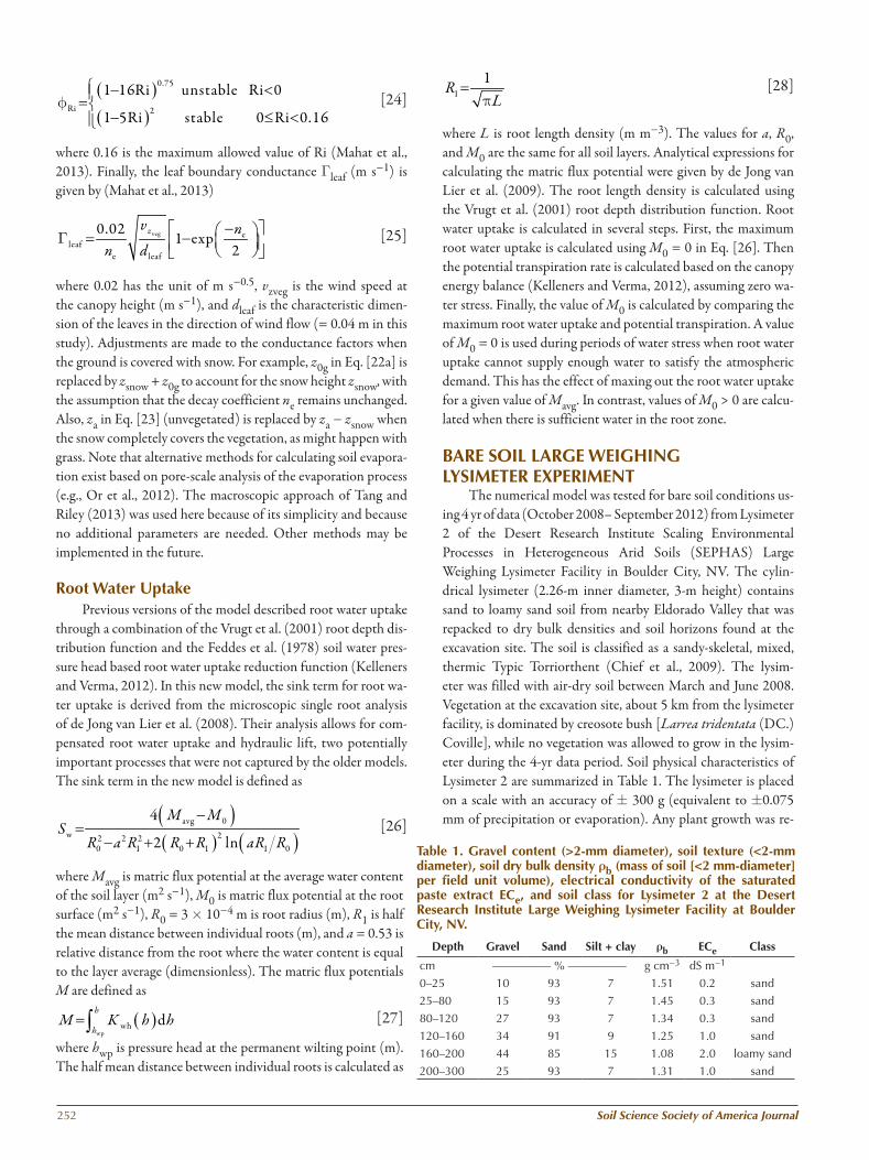
The numerical model was tested for bare soil conditions us-ing 4 yr of data (October 2008– September 2012) from Lysimeter 2 of the Desert Research Institute Scaling Environmental Processes in Heterogeneous Arid Soils (SEPHAS) Large Weighing Lysimeter Facility in Boulder City, NV. The cylin-drical lysimeter (2.26-m inner diameter, 3-m height) contains sand to loamy sand soil from nearby Eldorado Valley that was repacked to dry bulk densities and soil horizons found at the excavation site. The soil is classified as a sandy-skeletal, mixed, thermic Typic Torriorthent (Chief et al., 2009). The lysim-eter was filled with air-dry soil between March and June 2008. Vegetation at the excavation site, about 5 km from the lysimeter facility, is dominated by creosote bush [Larrea tridentata (DC.) Coville], while no vegetation was allowed to grow in the lysim-eter during the 4-yr data period. Soil physical characteristics of Lysimeter 2 are summarized in Table 1. The lysimeter is placed on a scale with an accuracy of ± 300 g (equivalent to ±0.075 mm of precipitation or evaporation). Any plant growth was re-

Table 1. gravel content (>2-mm diameter), soil texture (<2-mm diameter), soil dry bulk density rb (mass of soil [<2 mm-diameter] per field unit volume), electrical conductivity of the saturated paste extract ECe, and soil class for Lysimeter 2 at the Desert Research Institute Large Weighing Lysimeter Facility at Boulder City, NV.

Depth gravel Sand Silt + clay rb ECe Class

cm ————— % ————— g cm−3 dS m−1

0–25 10 93 7 1.51 0.2 sand

25–80 15 93 7 1.45 0.3 sand

80–120 27 93 7 1.34 0.3 sand

120–160 34 91 9 1.25 1.0 sand

160–200 44 85 15 1.08 2.0 loamy sand

200–300 25 93 7 1.31 1.0 sand


moved by hand each spring and weighed. The associated plant mass was within the accuracy range of the lysimeter scale and no corrections were made to the lysimeter weight. Measured deep percolation from the bottom of the lysimeter was zero during the 4-yr study period. More details on the construction, layout, and operation of the lysimeter were provided by Chief et al. (2009).

The climate at Boulder City, NV (elevation 770 m above mean sea level), is characterized by low precipitation (141-mm annual average) and warm temperatures (13.7°C average an-nual minimum temperature; 25.4°C average annual maximum temperature) according to the closest Western Regional Climate Center meteorological station no. 261071. Half-hourly weather data (humidity, temperature, wind speed, atmospheric pressure, and precipitation) for the 4-yr calculation period were available from a weather station at the lysimeter facility. Fractional cloud cover was derived from the National Climatic Data Center sta-tion data for Henderson Executive Airport (about 16 km to the west of Boulder City at 750 m above mean sea level). Atmospheric turbidity data needed for the calculation of aerosol optical depth (Kelleners et al., 2009) were derived from monthly solar radiation data from Desert Rock, NV (Augustine et al., 2008).

Only the top 250 cm of soil in the lysimeter was modeled because no sensor observations were conducted below this depth. Vertical grid spacing was 1 cm throughout the modeled domain. Soil water retention parameters for all six soil layers were deter-mined at the University of Wyoming. Water retention in the dry soil range was measured using a WP4 dew-point potentiometer (Decagon Devices). Water retention in medium wet soil (−7 < h < −1 m) was measured using Tempe cells and the pressure-outflow method (Dane and Hopmans, 2002a). Water retention in wet soils (h > −1 m) was measured using hanging water col-umns (Dane and Hopmans, 2002b). Repacked soil was used in all cases. Gravimetric water contents were converted to volumet-ric water contents using the bulk density values of the lysimeter soil layers (mass of soil [<2-mm diameter] per field unit volume; Russo [1983]; Table 1). Saturated volumetric water content as calculated for the lysimeter soil layers was also included as a data point. Optimum values for qwr, f, a, and n were determined us-ing the solver tool in Microsoft Excel. The resulting parameters are shown in Table 2. Saturated hydraulic conductivity Kwhs was set at 100 cm d−1 for all soil layers based on unpublished results from tension infiltration experiments conducted by the Desert Research Institute. Finally, the exponent l (Eq. [11a]) was fixed at 0.5 as recommended by Mualem (1976).

The top boundary condition for both water flow and heat transport was determined by the incoming precipitation and the surface energy balance (Kelleners et al., 2009). The bottom boundary condition for water flow was free drainage. The bottom boundary condition for heat transport was a prescribed tempera-ture as measured by a Model 229 Heat Dissipation Unit (HDU, Campbell Scientific) at the 250-cm depth. Our preferred bottom boundary condition for heat transport of a zero temperature gra-dient did not work well because the lower part of the lysimeter is situated in an underground chamber. This setup conflicts with

the assumption of an infinite soil profile and strictly vertical heat transport. This is reflected in the measured soil temperatures in the lysimeter, which show only a muted time lag with depth in re-sponse to seasonal changes in the surface energy balance. With the prescribed temperature boundary condition, the heat transport in the lower part of the lysimeter is more constrained, allowing the model to better capture the observed temperature dynamics. Initial conditions for water flow and heat transport were deter-mined using time domain reflectometry TDR 100–CS 605 water content data (Campbell Scientific) and HDU temperature data measured at the 5- (HDU only), 10-, 25-, 50-, 75-, 100-, 150-, 200-, and 250-cm depths. No parameter optimization was conducted for this study and the model was run using only default values.

Measured and calculated soil water content and soil tem-perature are shown in Fig. 2 and 3, respectively, for the 10-, 25-, 50-, 100-, and 150-cm depths. Measured and calculated lysim-eter liquid water gain and weekly bare soil evaporation are shown in Fig. 4, with the measured values being derived from the ly-simeter mass change with time. Measured and calculated bare soil evaporation rates were compared only for periods without precipitation to eliminate the impact of discrepancies between rain-gauge-measured and lysimeter-captured rainfall on the cal-culated and measured evaporation rates, respectively. Weekly evaporation rates were preferred over daily evaporation rates to increase the signal/noise ratio in the measured evaporation rates (measurement accuracy ± 0.075 mm). The calculated liquid wa-ter gain and evaporation in Fig. 4 are shown for the complete model (top row), for the model without vapor flow (Kvh = KvT = 0; middle row), and for the model without surface resistance (Gv

−1 = Gw−1 » 0; bottom row).

The modeling statistics for the complete model with vapor flow and surface resistance are summarized in Table 3, where the root mean square error (RMSE) and ME are as defined by Green and Stephenson (1986). The maximum value for ME is 1. The model-calculated values are worse than simply using the mea-sured mean when ME is <0. No modeling statistics are presented for lysimeter liquid water gain because later gain values are influ-enced by earlier gain values and therefore cannot be considered as independent values.

The ME values were variable for soil water content (0.32 £ ME £ 0.75), relatively high for soil temperature (0.87 £

Table 2. Residual water content qwr, porosity f, and the shape parameters a and n in the van genuchten (1980) soil water retention function for the six soil layers of Lysimeter 2 at the Desert Research Institute Large Weighing Lysimeter Facility at Boulder City, NV.

Depth qwr f a n

cm cm−1

0–25 0.022 0.341 0.0373 1.567

25–80 0.027 0.294 0.0209 1.790

80–120 0.041 0.280 0.0269 1.888

120–160 0.025 0.260 0.0300 1.621

160–200 0.011 0.242 0.0870 1.283

200–300 0.032 0.337 0.0745 1.626


ME £ 0.91), and intermediate for weekly bare soil evaporation (ME = 0.41). Figures 2 and 4 show that the lysimeter was gaining water while the soil moved toward a dynamic equilibrium after being packed dry between March and June 2008. In October 2012, at the end of the 4-yr simulation period, the wetting front was somewhere between the 200- and 250-cm depths (measured water contents not shown). The occasional significant dips in the calculated water contents at the 10-cm depth in Fig. 2 are due to short freezing events in winter when liquid water was trans-formed into ice. The two large “measured” condensation events in Fig. 4 (right column) may be due in part to missed precipita-tion events.

The soil temperatures were underestimated, especially dur-ing winter periods (Fig. 3). It appears that the chamber environ-ment was keeping the measured temperatures artificially high during winter. The one-dimensional vertical model was unable to capture the true three-dimensional lysimeter environment, de-spite the prescribed temperatures that define the bottom bound-ary condition for heat transport. The change in lysimeter mass,

expressed as liquid water gain in millimeters, due to incoming water from precipitation and outgoing water from evaporation was captured reasonably well by the model (Fig. 4, top left pan-el). The measured gain was 111 mm while the calculated gain was 95 mm during the 4-yr period. One contributing factor to the difference is that the lysimeter, with a surface area of 4 m2, is more efficient at capturing precipitation than the rain gauge, which typically suffers from under-catch (Duchon and Biddle, 2010). A good example of this can be seen for December 2010 in Fig. 4, top left panel, when the measured liquid water gain during a period of high precipitation was significantly higher than the calculated gain.

Calculated evaporation rates for May to June were gener-ally underestimated (Fig. 4, top right panel). This is also evident from Fig. 2, where calculated water contents at the 10- and 25-cm depths are consistently overestimated during May to June. It is difficult to determine whether these discrepancies were due to deficiencies in the surface energy balance equations, the coupled water flow–heat transport equations, the measured soil hydrau-

Fig. 2. Measured (black line) and calculated (complete model, gray line) soil water content at five depths for October 2008 to September 2012 for Lysimeter 2 of the Desert Research Institute Large Weighing Lysimeter Facility in Boulder City, NV.


lic properties, the Tang and Riley (2013) conductance factors, or a combination of these. Exclusion of vapor flow degraded the calculated evaporation rates, with ME decreasing from 0.41 (Fig. 4, top right panel) to ME = 0.37 (Fig. 4, middle right panel). Exclusion of surface resistance also degraded the evaporation rates, with ME decreasing to 0.36 (Fig. 4, bottom right panel). In addition, the RMSE increased from 1.20 mm wk−1 for the complete model to 1.25 mm wk−1 for both cases, confirming the reduced model performance. The underestimation of May to June evaporation rates even for the case without surface re-sistance (Fig. 4, bottom right panel) is surprising and requires further work, which was beyond the scope of the current study.

RANgELAND SOIL FIELD ExPERIMENTThe numerical model was also applied to a semiarid mixed-

grass rangeland near Laramie, WY (elevation 2200 m above sea level, average annual temperature 4.7°C, average annual precipi-tation 300 mm). The soil at the study site is a fine-loamy, mixed, superactive, frigid Ustic Calciargid, developed in alluvium on an

old Pleistocene terrace of the Laramie River. Soil texture ranges from sandy loam for the top 10 cm to loam and sandy clay loam at depth. High percentages of CaCO3 are found in the subsur-face. The vegetation consists mainly of cool-season grasses and is dominated by Sandberg bluegrass (Poa secunda J. Presl), prai-rie June grass [Koeleria macrantha (Ledeb.) Schult.], and west-ern wheatgrass [Elymus smithii (Rydb.) Barkworth and D.R. Dewey]. The site is grazed by both sheep (Ovis aries) and cows (Bos taurus) during short periods of the summer. A detailed de-scription of the soil physical characteristics and the soil hydrau-lic properties for this site were provided by Kelleners and Verma (2012).

An older version of the model was applied to the same site for the July 2009 to October 2011 period (Kelleners and Verma, 2012; Kelleners, 2013). For the current study, the simulation period was extended to cover 5 yr ( July 2009–September 2014). Climate data for 15-min intervals were from the Automated Surface Observation System (ASOS) at Laramie regional airport ?1 km from the site. Winter pre-

Fig. 3. Measured (black line and black circles) and calculated (complete model, gray line) soil temperature at five depths for October 2008 to September 2012 for Lysimeter 2 of the Desert Research Institute Large Weighing Lysimeter Facility in Boulder City, NV. The black circles are used for periods with infrequent (>3-h time interval) temperature measurements.


cipitation data were corrected using daily manual observations from the Community Collaborative Rain, Hail, and Snow (CoCoRaHS) network. Atmospheric turbidity was estimated from average monthly values for Cheyenne, WY, as presented by Curtis and Grimes (2004). The parameters in the Vrugt et al. (2001) root depth distribution function were changed com-pared with those of Kelleners and Verma (2012) to correct an error and to improve performance for the 5-yr period. The new values are: maximum rooting depth zm = 1.0 m; dimensionless empirical factor Pz = −5; empirical parameter z* = 1.0 m. In ad-dition, a vegetation height of 0.4 m, a maximum leaf area index (LAI) of 1.7 m2 m−2, and a soil profile root mass of 1.4 kg m−2 was assumed ( Jackson et al., 1996).

The simulated 3-m-deep soil profile had five diagnostic layers and was described using 52 nodes with grid spacing in-creasing from 1 cm at the surface to 50 cm in the subsurface. Soil hydraulic properties for the five layers were similar to those

reported by Kelleners and Verma (2012). The top boundary condition was again the result of incoming precipitation and the surface energy balance. The bottom boundary condition for water flow was free drainage. The bottom boundary condi-tion for heat transport was a zero temperature gradient. The initial conditions for water flow and heat transport as deter-mined from HydraProbe impedance–temperature sensors at the 7.5-, 15-, 25-, 45-, and 65-cm depths (Stevens Water Monitoring Systems) also remained unaltered compared with the previous studies. No additional parameter optimization was conducted for the present study.

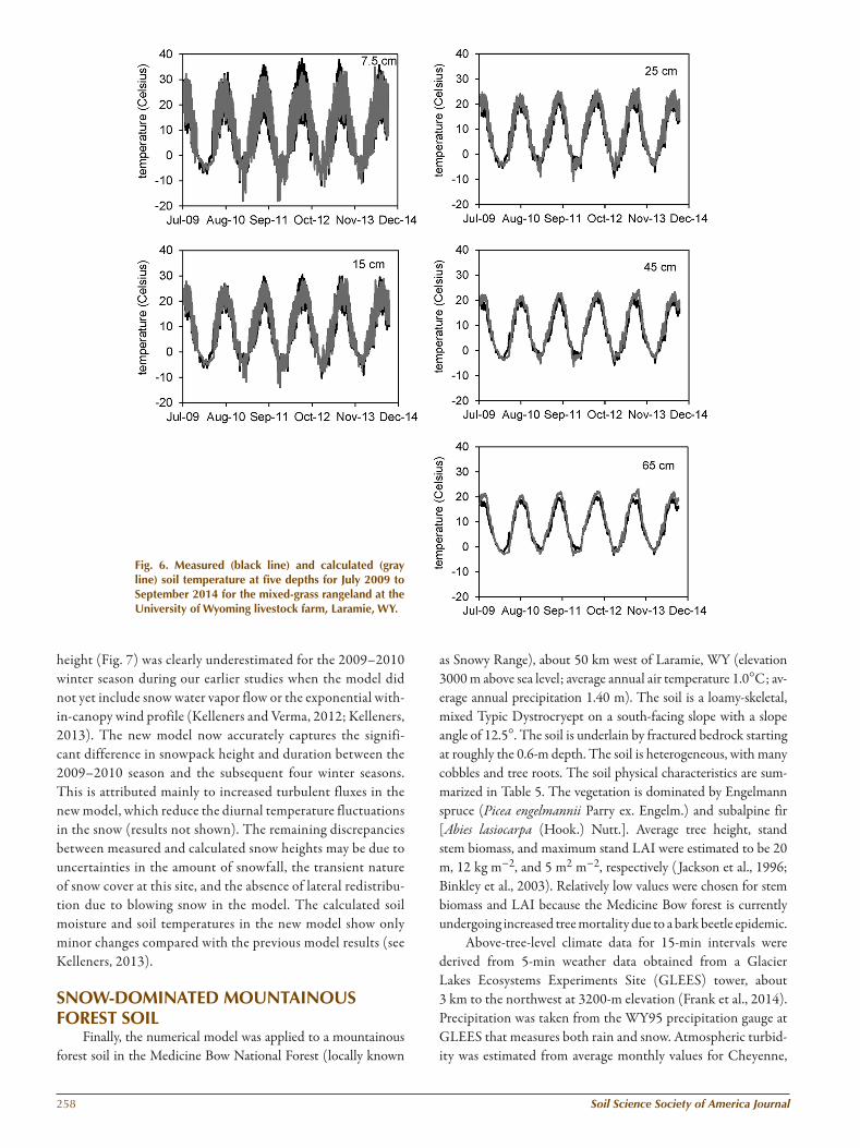
Measured and calculated soil water content, soil tempera-ture, and snow height are shown in Fig. 5, 6, and 7, respectively, where the measured snow heights were observed manually at 30-d intervals using a meter stick. The modeling statistics are sum-marized in Table 4. The model performance was variable, with good performance for soil temperature (0.92 £ ME £ 0.94),

Fig. 4. Measured (black line) and calculated (gray line) liquid water gain and bare soil evaporation rate for October 2008 to September 2012 for Lysimeter 2 of the Desert Research Institute Large Weighing Lysimeter Facility in Boulder City, NV. Calculated values are shown for the complete model (top row), without vapor flow (middle row), and without surface resistance (bottom row). The measured liquid water gain and bare soil evaporation rate were derived from the lysimeter mass change with time. Measured and calculated weekly evaporation rates are shown only for periods without precipitation.


intermediate performance for snow height (ME = 0.57), and relatively weak performance for soil water content (0.05 £ ME £ 0.30). These modeling statistics are similar to those of our previ-ous studies, which used only 2 yr of data (Kelleners and Verma, 2012; Kelleners, 2013). The RMSE values for soil water contents of 0.03 to 0.04 m3 m−3 are only slightly above the measurement accuracy of ±0.03 m3 m−3 for the HydraProbe (e.g., Kammerer et al., 2014), suggesting that soil spatial heterogeneity and sensor calibration are significant contributing factors to the discrepan-cies between measured and calculated soil water content.

Systematic discrepancies between measured and calculated soil water content occurred mainly for the 45- and 65-cm depths (Fig. 5). The water content was generally overestimated at these depths. This was probably due to imperfections in the soil hy-draulic properties (which were measured) and/or vegetation parameters (only partly based on measurements), in addition to the effects of soil spatial heterogeneity and sensor calibration as mentioned above. The calculated steep drops in (liquid) soil water content in winter were due to soil water freezing. These drops can also be observed in the measured values, albeit only when winter water contents were relatively high at the onset of freezing. Note that impedance probes, like most electromagnetic

soil water content sensors, mainly react to liquid water content (relative permittivity ?80) and not so much to ice (relative per-mittivity ?3).

The good model performance for soil temperature (Fig. 6) suggests that the calculated canopy and surface energy bal-ances are realistic for the mixed-grass ecosystem. Both the diurnal and seasonal trends were captured accurately. Snow

Table 3. Model statistics of root mean square error (RMSE) and modeling efficiency (ME) for soil water content, soil tem-perature, and the bare soil evaporation rate for October 2008 to September 2012 for Lysimeter 2 of the Desert Research Institute Large Weighing Lysimeter Facility in Boulder City, NV.

Depth Soil water content

Soil temperature

Bare soil evaporation

RMSE ME RMSE ME RMSE ME

cm m3 m−3 °C mm wk−1

Surface 1.2 0.41

10 0.02 0.56 3.3 0.91

25 0.02 0.32 3.0 0.89

50 0.01 0.75 3.1 0.87

100 0.02 0.41 2.6 0.87

150 0.01 0.75 2.3 0.87

Fig. 5. Measured (black line) and calculated (gray line) soil water content at five depths for July 2009 to September 2014 for the mixed-grass rangeland at the University of Wyoming livestock farm, Laramie, WY.


height (Fig. 7) was clearly underestimated for the 2009–2010 winter season during our earlier studies when the model did not yet include snow water vapor flow or the exponential with-in-canopy wind profile (Kelleners and Verma, 2012; Kelleners, 2013). The new model now accurately captures the signifi-cant difference in snowpack height and duration between the 2009–2010 season and the subsequent four winter seasons. This is attributed mainly to increased turbulent fluxes in the new model, which reduce the diurnal temperature fluctuations in the snow (results not shown). The remaining discrepancies between measured and calculated snow heights may be due to uncertainties in the amount of snowfall, the transient nature of snow cover at this site, and the absence of lateral redistribu-tion due to blowing snow in the model. The calculated soil moisture and soil temperatures in the new model show only minor changes compared with the previous model results (see Kelleners, 2013).

SNOW-DOMINATED MOUNTAINOUS FOREST SOIL

Finally, the numerical model was applied to a mountainous forest soil in the Medicine Bow National Forest (locally known

as Snowy Range), about 50 km west of Laramie, WY (elevation 3000 m above sea level; average annual air temperature 1.0°C; av-erage annual precipitation 1.40 m). The soil is a loamy-skeletal, mixed Typic Dystrocryept on a south-facing slope with a slope angle of 12.5°. The soil is underlain by fractured bedrock starting at roughly the 0.6-m depth. The soil is heterogeneous, with many cobbles and tree roots. The soil physical characteristics are sum-marized in Table 5. The vegetation is dominated by Engelmann spruce (Picea engelmannii Parry ex. Engelm.) and subalpine fir [Abies lasiocarpa (Hook.) Nutt.]. Average tree height, stand stem biomass, and maximum stand LAI were estimated to be 20 m, 12 kg m−2, and 5 m2 m−2, respectively ( Jackson et al., 1996; Binkley et al., 2003). Relatively low values were chosen for stem biomass and LAI because the Medicine Bow forest is currently undergoing increased tree mortality due to a bark beetle epidemic.

Above-tree-level climate data for 15-min intervals were derived from 5-min weather data obtained from a Glacier Lakes Ecosystems Experiments Site (GLEES) tower, about 3 km to the northwest at 3200-m elevation (Frank et al., 2014). Precipitation was taken from the WY95 precipitation gauge at GLEES that measures both rain and snow. Atmospheric turbid-ity was estimated from average monthly values for Cheyenne,

Fig. 6. Measured (black line) and calculated (gray line) soil temperature at five depths for July 2009 to September 2014 for the mixed-grass rangeland at the University of Wyoming livestock farm, Laramie, WY.


WY, as presented by Curtis and Grimes (2004). Air tempera-ture, relative humidity, atmospheric pressure, precipitation, and turbidity data were corrected for differences in elevation. The parameters in the Vrugt et al. (2001) root depth distribution function were zm = 0.6 m, Pz = 1, and z* = 0.6 m, resulting in a square-shaped distribution. Note that the maximum root-ing depth for temperate coniferous forest averages 3.9 ± 0.4 m (Canadell et al., 1996) but that the bulk of the roots are mostly in the top 0.5 m of the soil ( Jackson et al., 1996). The result-ing distribution, with a high root concentration between 0 and 0.6 m and few roots between 0.6 and 3.9 m, cannot be captured accurately with the Vrugt et al. (2001) function, despite its ver-satility. We therefore elected to limit the modeled root zone to 0.6 m to at least capture the high root concentration in the top 0.6 m. The mass of roots, needed to calculate the root length density L, was estimated at 4.4 kg m−2 ( Jackson et al., 1996).

The soil and underlying bedrock were modeled using four layers. The 0.6-m soil profile was described using three layers, each 20 cm in thickness. The underlying bedrock was described using one layer up to a depth of 10 m below the soil surface. A total of 81 nodes was used, with a grid spacing of 1 cm in the soil layers (requir-ing 60 nodes) and a gradually increasing grid spacing with depth of up to 2.1 m for the bedrock (requiring 21 nodes). Water reten-tion for the three soil layers was determined at the University of Wyoming (Table 6). Water retention in the dry soil range was mea-sured using a WP4 dew-point potentiometer (Decagon Devices). Water retention in medium wet soil (−10 < h < −1 m) was mea-

sured using a pressure plate apparatus (Dane and Hopmans, 2002c) and by subjecting Tempe cells to the pressure-outflow method (Dane and Hopmans, 2002a). Water retention in wet soils (h > −1 m) was measured using hanging water columns (Dane and Hopmans, 2002b). Repacked soil was used in all cases. Conversion of gravimetric to volumetric water contents was conducted using estimated dry bulk density values (mass of soil [<2-mm diameter] per field unit volume, Table 5) to scale the water retention data so that the model captured the field-measured volumetric soil water contents in the heterogeneous soil. The saturated soil hydraulic conductivity and pore connectivity values were estimated at 25 cm d−1 and 0.5, respectively. The hydraulic properties of the fractured bedrock in Table 6 were all estimated using a low value for porosity, a relatively high value for a (early air entry on drying), and a rela-tively high value for Kwhs (pore connectivity = 0.5).

The simulation period covered August 2009 to September 2014. The top boundary condition in the model was again due to precipitation and the surface energy balance. The bot-tom boundary condition for water flow and heat transport was free drainage and a zero temperature gradient, respectively. Soil and snow monitoring at the site started in October 2009 when there was already some snow on the ground. The soil environ-ment was monitored using HydraProbe impedance–tempera-ture sensors at 10, 30, and 50 cm below the soil surface (Stevens Water Monitoring Systems). Snow height was monitored using a downward-facing SR50 acoustic distance sensor (Campbell Scientific). Initiating the simulation period in August instead of October has the benefit of well-defined soil conditions. At this stage in the season, the soil is generally dry and warm and the ice content is zero. Also, snow cover is unlikely. The initial soil con-ditions for August 2009 were estimated by using a preliminary model run and by taking the soil conditions for August 2014 as the initial conditions for August 2009.

Fig. 7. Measured (symbols) and calculated (line) snow height for July 2009 to September 2014 for the mixed-grass rangeland at the University of Wyoming livestock farm, Laramie, WY.

Table 4. Model statistics of root mean square error (RMSE) and modeling efficiency (ME) for soil water content, soil tem-perature, and snow height for July 2009 to September 2014 for the mixed-grass rangeland at the University of Wyoming livestock farm, Laramie, WY.

Depth

Soil water content Soil temperature Snow height

RMSE ME RMSE ME RMSE ME

cm m3 m−3 °C m

Surface 0.05 0.57

7.5 0.04 0.30 2.9 0.92

15 0.04 0.20 2.4 0.94

25 0.03 0.28 2.4 0.93

45 0.04 0.12 2.1 0.93

65 0.04 0.05 2.0 0.93

Table 5. Measured soil texture (<2-mm diameter), estimated soil dry bulk density rb (mass of soil [<2-mm diameter] per field unit volume), and soil class for the south-facing moun-tainous forest site in the Medicine Bow National Forest, about 50 km west of Laramie, WY.

Depth Sand Silt Clay rb Class

cm ————— % ————— g cm−3

0–20 50 37 13 1.0 loam

20–40 50 35 15 0.7 loam

40–60 41 40 19 1.2 loam

Table 6. Residual water content qwr, porosity f, the shape parameters a and n in the van genuchten (1980) soil water retention function, and saturated hydraulic conductivity Kwhs for the three soil layers and the underlying fractured bedrock at the south-facing mountainous forest site in the Medicine Bow National Forest, about 50 km west of Laramie, WY.

Depth qwr f a n Kwhs

cm cm−1 cm d−1

0–20 0.0 0.351 0.038 1.277 25

20–40 0.0 0.218 0.030 1.280 25

40–60 0.0 0.440 0.074 1.261 25

60–1000 0.0 0.050 0.100 1.500 700


Measured and calculated soil water content, soil tempera-ture, and snow height are shown in Fig. 8, 9, and 10, respectively. The modeling statistics are summarized in Table 7. The ME values were highest for soil temperature (0.85 £ ME £ 0.88), intermediate for snow height (ME = 0.57), and lowest for soil water content (0.06 £ ME £ 0.37). The soils at this site are heterogeneous with many cobbles and large roots. It’s there-fore unrealistic to expect a perfect fit between measured and calculated soil water content. The relatively high RMSE values

for soil water content, between 0.05 and 0.07 m3 m−3, reflect this as well. Large systematic errors in the calculated soil water contents can be observed during the spring melt in April to May 2011 and April to May 2014 (Fig. 8). The measured water con-tents increased with time, presumably due to incoming meltwa-ter from the overlying snowpack. In contrast, the calculated soil water contents decreased due to a combination of limited snow meltwater input and gradually increasing root water uptake. The calculated average snow temperature during these periods was −2 to −3°C, while the actual snowpack was probably isothermal.

The calculated snow height was significantly overestimated in the 2010–2011 winter. The overestimate was a little less se-vere than suggested by Fig. 10 because the actual snow height ex-

Fig. 8. Measured (black line) and calculated (gray line) soil water content at three depths for August 2009 to September 2014 for the south-facing mountainous forest site in the Medicine Bow National Forest, about 50 km west of Laramie, WY. The two vertical arrows in the top panel (10 cm) indicate April to May 2011 and April to May 2014, respectively, when soil water contents are significantly underestimated by the model.

Fig. 9. Measured (black line) and calculated (gray line) soil temperature at three depths for August 2009 to September 2014 for the south-facing mountainous forest site in the Medicine Bow National Forest, about 50 km west of Laramie, WY.


ceeded the sensor height during this period, resulting in missing measured values. However, snow heights above 4 m probably did not occur. The high calculated snow heights are almost cer-tainly due to the GLEES area, which served as the source for the precipitation data, receiving more snowfall than the study site. For example, a snow height of 3.8 m was measured manually at GLEES in April 2011. We applied a generic elevation correc-tion to precipitation that did not capture the large differences in snow input between GLEES and our site during this event. Note that the non-zero height readings of up to 0.4 m during the summer periods are due to the acoustic sensor signal reflec-tion of understory vegetation. The measured snow height was set to zero for the months of July and August for the calculation of RMSE and ME because snow cover is unlikely during these 2 mo. The understory vegetation was not simulated in the present model application.

Small systematic differences between measured and calculated soil temperatures can also be observed (Fig. 9). The calculated soil temperature at the 10-cm depth was often underestimated during the summer months. This may be due to the canopy energy balance method being used where Beer’s law is used to calculate the fraction of solar radiation that is being intercepted by the canopy. In reality, portions of the solar radiation beam may reach the surface without being intercepted because the canopy is not completely closed. This results in some locations being warmer than expected. This type of overestimation is most likely in the summer when the sun is relatively high in the sky. Vegetation change due to the ongoing bark beetle epidemic may also be a contributing factor. The delay in calculated soil warmup in June and July 2011 for all depths is due to the delayed melt of the snowpack for the 2010–2011 winter owing to the likely overestimation of snowfall during February 2011, as mentioned above.

CONCLUSIONSThe numerical model for coupled water flow and heat trans-

port in soil and snow was applied to a warm bare desert lysimeter soil, a cold mixed-grass rangeland soil, and a snow-dominated

mountainous forest soil. The combined simulation periods to-taled >14 yr. Results for the bare lysimeter soil showed that the lysimeter mass change due to incoming precipitation and out-going evaporation, expressed as liquid water gain, was captured reasonably well by the model (measured gain = 111 mm; calcu-lated gain = 95 mm; ME for bare soil evaporation = 0.41). The comparison of measured vs. calculated soil temperatures was hampered by the lysimeter design, which allows three-dimen-sional heat transport that deviates from the one-dimensional heat transport as assumed by the model. Model performance for soil temperature was best for the mixed-grass rangeland soil, with ME ³ 0.92 for all five depths. The model’s ability to simulate realistic snowpack heights was demonstrated for both the range-land soil and the mountainous forest soil, where snow height was calculated with ME = 0.57 for both sites.

Calculating realistic soil water contents is a challenge and ME values varied considerably in this study, with 0.32 £ ME £ 0.75 for the bare soil, 0.05 £ ME £ 0.30 for the rangeland soil, and 0.06 £ ME £ 0.37 for the forest soil. Calculated water con-tents are sensitive to the prescribed soil water retention curves, which were measured in the laboratory. However, the transla-tion to actual field conditions is challenging due to variations in gravel content (lysimeter soil), the presence of a dense CaCO3 layer (rangeland soil), and the presence of cobbles and large roots (forest soil). The process of hysteresis and the presence of mac-ropores (neither included in the model) further add to the chal-lenge, as do uncertainties about soil water sensor calibration and the distribution and activity of roots. It’s conceivable that the soil water ME values can be improved by optimizing the soil hy-draulic (all three sites) and the vegetation parameters (rangeland and forest sites) using an inverse algorithm. This was beyond the scope of the current study but could be attempted in the future.

Overall, though, the model presented in this study was able to calculate realistic soil water contents for all three ecosystems. Advantages of the current model are the inclusion of all three water phases (ice, liquid, and vapor) in a physics-based approach, a realistic within-canopy exponential wind profile (Dolman, 1993), the inclusion of compensated root water uptake (de Jong van Lier et al., 2008), and the absence of an empirical reduction factor for soil evaporation (van de Griend and Owe, 1994; Tang and Riley, 2013). These attributes should allow application of the model to a variety of terrestrial ecosystems without the need

Fig. 10. Measured (black line) and calculated (gray line) snow height for August 2009 to September 2014 for the south-facing mountainous forest site in the Medicine Bow National Forest, about 50 km west of Laramie, WY.

Table 7. Model statistics of root mean square error (RMSE) and modeling efficiency (ME) for soil water content, soil tem-perature, and snow height for August 2009 to September 2014 for the south-facing mountainous forest site in the Medicine Bow National Forest, about 50 km west of Laramie, WY.

Depth

Soil water content Soil temperature Snow height

RMSE ME RMSE ME RMSE MEcm m3 m−3 °C m

Surface 0.33 0.57

10 0.06 0.37 1.9 0.85

30 0.05 0.24 1.5 0.88

50 0.07 0.06 1.3 0.88


for prior assumptions about the dominant processes. A disadvan-tage of the model is the computational effort required to solve the coupled water flow and heat transport equations, and re-search to solve these equations more efficiently is ongoing.

APPENDIx: DERIVATIVE TERMSThe derivative of liquid water content qw (m3 m−3) with

respect to relative saturation Se (dimensionless) for snow is

( ) ( )( )

( ) ( )( )

e c c c i i ww2

e e c c

c e e c i i w c i i w

2e c c

1 1dd 1

1

S F F F

S S F F

F S S F F

S F F

é ù+ - - q r rq ê úë û=+ -

é ù- q r r + q r rê úë û-+ -

[A1]

where Fc is mass of liquid water that can be retained per mass of dry snow (kg kg−1), qi is ice content (m3 m−3), ri is ice density (kg m−3), and rw is liquid water density (kg m−3). The derivative of soil water surface tension g (kg s−2) with respect to tempera-ture T (°C) is (Bachmann and van der Ploeg, 2002)

d0.0001535

dTg=− [A2]

The derivative of qw with respect to soil water pressure head h (m) is (Mous, 1995; Radcliffe and Šimůnek, 2010)

( ) ( )

( )( )( ) ( )

1wr

1

w

1/wr e

11/e

1 , 0dd

1 1 , 0

nn

mn

m

mm

mn h

h hh m S

S m h

a f q

aq

a f q

−

− −

−

− − × + − < =

−

× − − ≥

[A3]

where a (m−1), n (dimensionless), and m (dimensionless) are empirical parameters in the van Genuchten (1980) water reten-tion function, f is porosity (m3 m−3), and qwr is residual liquid water content (m3 m−3). The derivative of relative humidity Hr (dimensionless) with respect to h is given by

( )w wr

r w2w

ddd 273.15 d

M gH H M Mh R T h

qfq

= + +

[A4]

where Mw is molecular mass of water (kg mol−1), g is accelera-tion due to gravity (m s−2), R is the gas constant ( J mol−1 K−1), and M is molality at saturation (mol kg−1 of solvent). The de-rivative of Hr with respect to T is

( )wr

r 2

ww2

w

0 snow

dd 273.15

dsoil, 0

d

hM gH HT R T

M M hTqf

q

−=

+ + ≤

[A5]

The derivative of qw with respect to T is (Kelleners, 2013)

( )

( )

22i i

2 2 22 2w

w f

w

1

2w w

2 11 snow, 0

11

d 1d 273.15

273.15dsoil, 0

d

a T Ta Ta T

RMT g T g

RM Th Tg

q rr

q g fq

fq q

−

−

− − < + + = + + +× + <

[A6]

where a = 1000°C−1 is a constant with reported values of 100 to 1000°C−1 (Jordan et al., 1999), and gf is the latent heat of fusion (J kg−1). Finally, drvs/dT over ice and water is calculated using sixth-order polynomials and data provided by Oleson et al. (2013).

ACKNOWLEDgMENTSThe SEPHAS large weighing lysimeter study is based on work supported by the National Science Foundation under Grant no. EPS-0447416. The field measurements at the mixed-grass rangeland site were facilitated by an equipment grant from the University of Wyoming Agricultural Experiment Station. Field data collection and modeling work at the mountainous forest site was supported by a University of Wyoming Faculty Grant-In-Aid award and by the National Science Foundation funded Wyoming Center for Environmental Hydrology and Geophysics under Grant no. EPS-1208909. The comments of three anonymous reviewers and the associate editor helped to improve the paper.

REFERENCESAugustine, J.A., G.B. Hodges, E.G. Dutton, J.J. Michalsky, and C.R. Cornwall.

2008. An aerosol optical depth climatology for NOAA’s national surface radiation budget network (SURFRAD). J. Geophys. Res. 113:D11204. doi:10.1029/2007JD009504

Bachmann, J., and R.K. van der Ploeg. 2002. A review of recent developments in soil water retention theory: Interfacial tension and temperature effects. J. Plant Nutr. Soil Sci. 165:468–478. doi:10.1002/1522-2624(200208)165:4<468::AID-JPLN468>3.0.CO;2-G

Binkley, D., U. Olsson, R. Rochelle, T. Stohlgren, and N. Nikolov. 2003. Structure, production and resource use in some old-growth spruce/fir forests in the Front Range of the Rocky Mountains, USA. For. Ecol. Manage. 172:271–279. doi:10.1016/S0378-1127(01)00794-0

Canadell, J., R.B. Jackson, J.R. Ehleringer, H.A. Mooney, O.E. Sala, and E.D. Schulze. 1996. Maximum rooting depth of vegetation types at the global scale. Oecologia 108:583–595. doi:10.1007/BF00329030

Cass, A., G.S. Campbell, and T.L. Jones. 1984. Enhancement of thermal water vapor diffusion in soil. Soil Sci. Soc. Am. J. 48:25–32. doi:10.2136/sssaj1984.03615995004800010005x

Celia, M.A., E.T. Bouloutas, and R.L. Zarba. 1990. A general mass-conservative numerical solution for the unsaturated flow equation. Water Resour. Res. 26:1483–1496. doi:10.1029/WR026i007p01483

Chief, K., M.H. Young, B.F. Lyles, J. Healey, J. Koonce, E. Knight, et al. 2009. Scaling environmental processes in heterogeneous arid soils: Construction of large weighing lysimeter facility. Publ. 41249. Desert Res. Inst., Las Vegas, NV.

Colbeck, S.C. 1993. The vapor diffusion coefficient for snow. Water Resour. Res. 29:109–115. doi:10.1029/92WR02301

Colbeck, S.C., and G. Davidson. 1973. Water percolation through homogeneous snow. In: International Symposium on the Role of Snow and Ice in Hydrology, Banff, AB, Canada. Sept. 1972. IAHS Publ. 107. Inst. of Hydrology, Wallingford, UK. p. 242–256.

Curtis, J., and K. Grimes. 2004. Wyoming climate atlas. Wyoming State Climatologist Office, Laramie.

Dall’Amico, M., S. Endrizzi, S. Gruber, and R. Rigon. 2011. A robust and energy-conserving model of freezing variably-saturated soil. Cryosphere 5:469–484. doi:10.5194/tc-5-469-2011

Dane, J.H., and J.W. Hopmans. 2002a. Pressure cell. In: J.H. Dane and G.C. Topp, editors, Methods of soil analysis. Part 4. Physical methods. SSSA Book Ser. 5. SSSA, Madison, WI. p. 684–688. doi:10.2136/sssabookser5.4.c25


Dane, J.H., and J.W. Hopmans. 2002b. Hanging water column. In: J.H. Dane and G.C. Topp, editors, Methods of soil analysis. Part 4. Physical methods. SSSA Book Ser. 5. SSSA, Madison, WI. p. 680–683. doi:10.2136/sssabookser5.4.c25

Dane, J.H., and J.W. Hopmans. 2002c. Pressure plate extractor. In: J.H. Dane and G.C. Topp, editors, Methods of soil analysis. Part 4. Physical methods. SSSA Book Ser. 5. SSSA, Madison, WI. p. 688–690. doi:10.2136/sssabookser5.4.c25

de Jong van Lier, Q., D. Dourado Neto, and K. Metselaar. 2009. Modeling of transpiration reduction in van Genuchten–Mualem type soils. Water Resour. Res. 45:W02422. doi:10.1029/2008WR006938

de Jong van Lier, Q., J.C. van Dam, K. Metselaar, R. de Jong, and W.H.M. Duijnisveld. 2008. Macroscopic root water uptake distribution using a matric flux potential approach. Vadose Zone J. 7:1065–1078. doi:10.2136/vzj2007.0083

Dolman, A.J. 1993. A multiple-source land surface energy balance model for use in general circulation models. Agric. For. Meteorol. 65:21–45. doi:10.1016/0168-1923(93)90036-H

Duchon, C.E., and C.J. Biddle. 2010. Undercatch of tipping-bucket gauges in high rain rate events. Adv. Geosci. 25:11–15. doi:10.5194/adgeo-25-11-2010

Fayer, M.J. 2000. UNSAT-H Version 3.0: Unsaturated soil water and heat flow model: Theory, user manual, and examples. Rep. 13249. Pac. Northw. Natl. Lab., Richland, WA.

Farouki, O.T. 1981. The thermal properties of soils in cold regions. Cold Reg. Sci. Technol. 5:67–75. doi:10.1016/0165-232X(81)90041-0

Feddes, R.A., P.J. Kowalik, and H. Zaradny. 1978. Simulation of field water use and crop yield. Simul. Monogr. Pudoc, Wageningen, the Netherlands.

Flerchinger, G.N. 2000. The Simultaneous Heat and Water (SHAW) model: Technical documentation. Tech. Rep. 2000-09. Northw. Watershed Res. Ctr., Boise, ID.

Flerchinger, G.N., and K.E. Saxton. 1989. Simultaneous heat and water model of a freezing snow–residue–soil system: I. Theory and development. Trans. ASAE 32:565–571. doi:10.13031/2013.31040

Frank, J.M., W.J. Massman, B.E. Ewers, L.S. Huckaby, and J.F. Negron. 2014. Ecosystem CO2/H2O fluxes are explained by hydraulically limited gas exchange during tree mortality from spruce bark beetles. J. Geophys. Res. 119:1195–1215. doi:10.1002/2013JG002597

Fuchs, M., G.S. Campbell, and R.I. Papendick. 1978. An analysis of sensible and latent heat flow in a partially frozen unsaturated soil. Soil Sci. Soc. Am. J. 42:379–385. doi:10.2136/sssaj1978.03615995004200030001x

Green, I.R.A., and D. Stephenson. 1986. Criteria for comparison of single event models. Hydrol. Sci. J. 31:395–411. doi:10.1080/02626668609491056

Guymon, G.L., and J.N. Luthin. 1974. A coupled heat and moisture transport model for arctic soils. Water Resour. Res. 10:995–1001. doi:10.1029/WR010i005p00995

Hansson, K., J. Šimůnek, M. Mizoguchi, L.-C. Lundin, and M.Th. van Genuchten. 2004. Water flow and heat transport in frozen soil: Numerical solution and freeze–thaw applications. Vadose Zone J. 3:693–704. doi:10.2136/vzj2004.0693

Harlan, R.L. 1973. Analysis of coupled heat–fluid transport in partially frozen soil. Water Resour. Res. 9:1314–1323. doi:10.1029/WR009i005p01314

Jackson, R.B., J. Canadell, J.R. Ehleringer, H.A. Mooney, O.E. Sala, and E.D. Schulze. 1996. A global analysis of root distributions for terrestrial biomes. Oecologia 108:389–411. doi:10.1007/BF00333714

Jordan, R. 1991. A one-dimensional temperature model for a snow cover: Technical documentation for SNTHERM.89. Spec. Rep. 91-16. U.S. Army Corps Eng., Cold Regions Res. Eng. Lab., Hanover, NH.

Jordan, R.E., E.L. Andreas, and A.P. Makshtas. 1999. Heat budget of snow-covered sea ice at North Pole 4. J. Geophys. Res. 104:7785–7806. doi:10.1029/1999JC900011

Kammerer, G., R. Nolz, M. Rodny, and W. Loiskandl. 2014. Performance of Hydra probe and MPS-1 soil water sensors in topsoil tested in lab and field. J. Water Resour. Prot. 6:1207–1219. doi:10.4236/jwarp.2014.613110

Kelleners, T.J. 2013. Coupled water flow and heat transport in seasonally frozen soils with snow accumulation. Vadose Zone J. 12(4). doi:10.2136/vzj2012.0162

Kelleners, T.J., D.G. Chandler, J.P. McNamara, M.M. Gribb, and M.S. Seyfried. 2009. Modeling the water and energy balance of vegetated areas with snow accumulation. Vadose Zone J. 8:1013–1030. doi:10.2136/vzj2008.0183

Kelleners, T.J., and A.K. Verma. 2012. Modeling carbon dioxide production and transport in a mixed-grass rangeland soil. Vadose Zone J. 11(3).

doi:10.2136/vzj2011.0205Mahat, V., D.G. Tarboton, and N.P. Molotch. 2013. Testing above- and below-

canopy representations of turbulent fluxes in an energy balance snowmelt model. Water Resour. Res. 49:1107–1122. doi:10.1002/wrcr.20073

Moene, A.F., and J.C. van Dam. 2014. Transport in the atmosphere–vegetation–soil continuum. Cambridge Univ. Press, New York.

Moldrup, P., T. Oleson, T. Yamaguchi, P. Schjonning, and D.E. Rolston. 1999. Modeling diffusion and reaction in soils: IX. The Buckingham–Burdine–Campbell equation for gas diffusivity in undisturbed soil. Soil Sci. 164:542–551. doi:10.1097/00010694-199908000-00002

Mous, S.L.J. 1995. An efficient solution procedure for the one-step experiment. Appl. Math. Model. 19:130–132. doi:10.1016/0307-904X(94)00006-R

Mualem, Y. 1976. A new model for predicting the hydraulic conductivity of unsaturated porous media. Water Resour. Res. 12:513–522. doi:10.1029/WR012i003p00513

Nassar, I.N., and R. Horton. 1989. Water transport in unsaturated nonisothermal salty soil: II. Theoretical development. Soil Sci. Soc. Am. J. 53:1330–1337. doi:10.2136/sssaj1989.03615995005300050005x

Nassar, I.N., and R. Horton. 1992. Simultaneous transfer of heat, water, and solute in porous media: I. Theoretical development. Soil Sci. Soc. Am. J. 56:1350–1356. doi:10.2136/sssaj1992.03615995005600050004x

Oleson, K.W., D.M. Lawrence, G.B. Bonan, B. Drewniak, M. Huang, C.D. Koven, et al. 2013. Technical description of Version 4.5 of the Community Land Model (CLM). Tech. Note TN-503+STR. Natl Ctr. Atmos. Res., Boulder, CO.

Or, D., P. Lehmann, E. Shahraeeni, and N. Shokri. 2012. Advances in soil evaporation physics: A review. Vadose Zone J. 12(4). doi:10.2136/vzj2012.0163

Painter, S.L. 2011. Three-phase numerical model of water migration in partially frozen geological media: Model formulation, validation, and applications. Comput. Geosci. 15:69–85. doi:10.1007/s10596-010-9197-z

Philip, J.R., and D.A. de Vries. 1957. Moisture movement in porous materials under temperature gradients. Trans. Am. Geophys. Union 38:222–232. doi:10.1029/TR038i002p00222

Pinzer, B.R., M. Schneebeli, and T.U. Kaempfer. 2012. Vapor flux and recrystallization during dry snow metamorphism under a steady temperature gradient as observed by time-lapse micro-tomography. Cryosphere 6:1141–1155. doi:10.5194/tc-6-1141-2012

Radcliffe, D.E., and J. Šimůnek. 2010. Soil physics with HYDRUS: Modeling and applications. CRC Press, Boca Raton, FL.

Russo, D. 1983. Leaching characteristics of a stony desert soil. Soil Sci. Soc. Am. J. 47:431–438. doi:10.2136/sssaj1983.03615995004700030008x

Saito, H., J. Šimůnek, and B.P. Mohanty. 2006. Numerical analysis of coupled water, vapor, and heat transport in the vadose zone. Vadose Zone J. 5:784–800. doi:10.2136/vzj2006.0007

Šimůnek, J., M. Sejna, H. Saito, M. Sakai, and M.Th. van Genuchten. 2013. The HYDRUS-1D software package for simulating the one-dimensional movement of water, heat, and multiple solutes in variably-saturated media. Version 4.16. Univ. of California, Riverside.

Shimizu, H. 1970. Air permeability of deposited snow. Contrib. 1053. Inst. Low Temp. Sci., Sapporo, Japan.

Tang, J.Y., and W.J. Riley. 2013. A new top boundary condition for modeling surface diffusive exchange of a generic volatile tracer: Theoretical analysis and application to soil evaporation. Hydrol. Earth Syst. Sci. 17:873–893. doi:10.5194/hess-17-873-2013

Tarboton, D.G., and C.H. Luce. 1996. Utah energy balance snow accumulation and melt model (UEB): Computer model technical description and users guide. Utah Water Res. Lab., Logan.

van de Griend, A.A., and M. Owe. 1994. Bare soil surface resistance to evaporation by vapor diffusion under semiarid conditions. Water Resour. Res. 30:181–188. doi:10.1029/93WR02747

van Genuchten, M.Th. 1980. A closed-form equation for predicting the hydraulic conductivity of unsaturated soils. Soil Sci. Soc. Am. J. 44:892–898. doi:10.2136/sssaj1980.03615995004400050002x

Vrugt, J.A., J.W. Hopmans, and J. Šimůnek. 2001. Calibration of a two-dimensional root water uptake model. Soil Sci. Soc. Am. J. 65:1027–1037. doi:10.2136/sssaj2001.6541027x

Zhao, L., D.M. Gray, and D.H. Male. 1997. Numerical analysis of simultaneous heat and mass transfer during infiltration into frozen ground. J. Hydrol. 200:345–363. doi:10.1016/S0022-1694(97)00028-0

Numerical modeling of coupled water flow and heat ... · Numerical Modeling of Coupled Water Flow...

Documents

Transcript of Numerical modeling of coupled water flow and heat ... · Numerical Modeling of Coupled Water Flow...