This is a repository copy of Numerical modeling of converging compound channel flow.

White Rose Research Online URL for this paper:http://eprints.whiterose.ac.uk/126633/

Version: Accepted Version

Article:

Naik, B, Khatua, KK, Wright, N et al. (2 more authors) (2018) Numerical modeling of converging compound channel flow. ISH Journal of Hydraulic Engineering, 24 (3). pp. 285-297. ISSN 0971-5010

https://doi.org/10.1080/09715010.2017.1369180

(c) 2017, Indian Society for Hydraulics. This is an Accepted Manuscript of an article published by Taylor & Francis in the ISH Journal of Hydraulic Engineering on 20 September 2017, available online: https://doi.org/10.1080/09715010.2017.1369180

eprints@whiterose.ac.ukhttps://eprints.whiterose.ac.uk/

Reuse

Items deposited in White Rose Research Online are protected by copyright, with all rights reserved unless indicated otherwise. They may be downloaded and/or printed for private study, or other acts as permitted by national copyright laws. The publisher or other rights holders may allow further reproduction and re-use of the full text version. This is indicated by the licence information on the White Rose Research Online record for the item.

Takedown

If you consider content in White Rose Research Online to be in breach of UK law, please notify us by emailing eprints@whiterose.ac.uk including the URL of the record and the reason for the withdrawal request.

Numerical modeling of Converging Compound Channel Flow 1

2

B. Naik1, K.K.Khatua2 N. G. Wright3, and A. Sleigh4 P. Singh5 3

4

1 Ph. D. Research Scholar, Department of Civil Engineering, National Institute of Technology 5

Rourkela, India. Email:banditanaik1982@gmail.com 6

2 Associate Professor, Department of Civil Engineering, National Institute of Technology Rourkela, 7

India. Email: kkkhatua@yahoo.com 8

3 Professor of Water and Environmental Engineering, University of Leeds, School of Civil 9

Engineering, UK. Email: n.g.wright@leeds.ac.uk 10

4 Professor, Department of Water and Environmental Engineering, University of Leeds, 11

School of Civil Engineering, UK. Email: p.a.sleigh@leeds.ac.uk 12

5 M.Tech Scholar, Department of Civil Engineering, National Institute of Technology Rourkela, India. 13

Email:prateek.k.singh1992@gmail.com 14

15

16

Abstract 17

18

This paper presents numerical analysis for prediction of depth-averaged velocity distribution of 19

compound channels with converging flood plains. Firstly, a 3D Computational Fluid Dynamics 20

(CFD) model is used to establish the basic database under various working conditions. 21

Numerical simulation in two phases is performed using the ANSYS-Fluent software. k-＼ 22

turbulence model is executed to solve the basic governing equations. The results have been 23

compared with high quality flume measurements obtained from different converging compound 24

channels in order to investigate the numerical accuracy. Then ANN (Artificial Neural Network) 25

are trained based on the Back Propagation Neural Network (BPNN) technique for depth-26

averaged velocity prediction in different converging sections and these test results are compared 27

with each other and with actual data. The study has focused on the ability of the software to 28

correctly predict the complex flow phenomena that occur in channel flows. 29

30

Keywords: compound channel, stage discharge, Prismatic, non-prismatic, ANN, ANSYS 31

32

1 INTRODUCTION 33

34

Distribution of depth-averaged velocity is important aspect in river hydraulics and engineering 35

problems in order to give a basic understanding of the resistance relationship, to understand the 36

mechanisms of sediment transport and to design sustainable channels etc. Due to continuous 37

settlement of people near the riverbank and due to natural causes, the channel with floodplain 38

cross-sections behaves as converging type non-prismatic compound channels. An improper 39

estimation of floods in these regions, will lead to an increase in the loss of life and property. A 40

number of authors [1-8] has investigated the depth-averaged velocity distribution and flow 41

resistance in prismatic compound cross-sections. These models are not appropriate to predictions 42

in compound channels with converging flood plain because of non-uniform flow occurs from 43

section to section. Therefore, there is a need to evaluate the depth-averaged velocity in the main 44

channel and floodplain at various locations of a converging compound channel. Converging 45

channel flows, being highly complicated, are a matter of recent and continued research. For a 46

better understanding of the structure of turbulent flow in converging compound channels, it is 47

necessary to undertake detailed measurements. Because of the difficulty in obtaining sufficiently 48

accurate and comprehensive field measurements of velocity and shear stress in converging 49

compound channels under non-uniform flow conditions, considerable reliance must still be 50

placed on well focused laboratory investigations under steady flow conditions to provide the 51

information concerning the details of the flow structures and lateral momentum transfer. 52

Attention must be paid to the fact that physical models are very expensive, especially when a 53

large number of influencing parameters have to be studied. Sometimes, it is impossible to 54

construct a physical model for certain prototypes. Therefore, there is urgent need for economic 55

mathematical prediction models. In past a lot of experimental research has been done on 56

prismatic compound channel flows but relatively less usage has been made of numerical 57

techniques on non-prismatic compound sections. After the development of powerful computers 58

and sophisticated CFD (Computational Fluid Dynamics) techniques, much research is now being 59

conducted using these techniques in different research areas. This is not only due to economy 60

and less time required with CFD methodology but also due to the fact that through CFD one can 61

cover those aspects of flow behavior which are very difficult to observe through 62

experimentation. In recent years, numerical modeling of open channel flows has successfully 63

reproduced experimental results. Computational fluid dynamics (CFD) has been used to model 64

open channel flows ranging from main channels to flood plains. Simulations have been 65

performed by Krishnappan & Lau (1986), Kawahara & Tamai (1988) and Cokljat (1993). CFD 66

has also been used to model flow features in natural rivers by Sinha et al. (1998), Lane et al. 67

(1999), and Morvan (2001). Hodskinson (1996, 1998) was one of the first to present results using 68

a commercial CFD. In this case FLUENT was used to predict the 3D flow structure in a 90-69

degree bend on the River Dean in Cheshire. Pan & Banerjee (1995), Hodges & Street (1999), 70

and Nakayama & Yokojima (2002) studied free surface fluctuations in open channel flow by 71

employing the LES method. Hsu et al. (2000) have reported the existence of the inner secondary 72

currents in the rectangular open-channels, which occur at the junction of the free surface and 73

sidewall. Knight et al. (2005) applied state-of-the-art CFD software to explore the physics within 74

open-channel flows. In their research work they applied three different turbulent models, namely 75

the k-似, Reynolds Stress model by Speziale, Sarkar and Gatski (SSG) by Speziale et al. (1991) 76

and Reynolds Stress の or SMC-の (implemented in ANSYS-CFX) models to trapezoidal channel. 77

Thomas and Williams (1995a) and Cater and Williams (2008) simulated an asymmetric 78

rectangular compound channel using LES for a relative depth of ɴ = 0.5. They have predicted 79

mean stream wise velocity distribution, secondary currents, bed shear stress distribution, 80

turbulence intensities, TKE, and calculated lateral distribution of apparent shear stress. Gandhi et 81

al. (2010) determined the velocity profiles in two directions under different real flow field 82

conditions and also investigated the effects of bed slope, upstream bend and a convergence / 83

divergence of channel width. Kara et al. (2012) compared the depth-averaged stream wise 84

velocities obtained by LES with calculated by analytical solution of Shiono and Knight Method 85

(SKM), and concluded that the analytical approach to their problem requires calibration of the 86

lateral eddy viscosity coefficient, そ, and the secondary current parameter, d. Xie et al. (2013) 87

used LES to simulate asymmetric rectangular compound channel. In this study the distributions 88

of the mean velocity and secondary flows, boundary shear stress, turbulence intensities, TKE and 89

Reynolds stresses were in a good agreement with the experimental data. Filonovich (2015) used 90

ANSYS-CFX package to allow the simulation of uniform flows in straight asymmetric 91

trapezoidal and rectangular compound channels with several different RANS turbulence closure 92

models. 93

94

In the last decade machine-learning methods were the subject of many researches in engineering 95

problems and also in water resources engineering (Cheng et al., 2002; Lin et al., 2006; 96

Muzzammil, 2008; Wang et al., 2009; Wu et al. 2009; Ghosh et al., 2010; Safikhani et al., 97

2011). Bilgil and Altun (2008) predicted friction factor in smooth open channel flow using ANN. 98

Sahu et al. (2011) proposed an artificial neural network model for accurate estimation of 99

discharge in compound channel flume and Moharana and Khatua (2014) studied the flow 100

resistance in meandering compound channels by using ANFIS. Abdeen (2008) adopted an ANN 101

technique to simulate the impacts of vegetation density, flow discharge and the operation of 102

distributaries on the water surface profile of open channels. Yuhong and Wenxin (2009) studied 103

the application of ANN for prediction of friction factor of open channel flows. The ANN 104

technique has also been successfully applied to compound open channel flow for the prediction 105

of the hydraulics characteristics, such as integrated discharge and stage-discharge relations 106

(Bhattacharya & Solomatine 2005; Jain 2008; Unal et al. 2010; Sahu et al.2011) 107

108

In the first part of this paper, 3D numerical simulations of flow field with two phases (water & 109

air) are carried out with the software ANSYS FLUENT to study the variation of velocity profiles 110

in different converging sections of a compound channel. In multiphase fluid flow, a phase is 111

described as a particular class of material that has a certain inertial response and interaction with 112

the fluid flow and the potential field in which it is immersed. Currently there are two approaches 113

for the numerical calculation of multiphase flows: The Euler-Lagrange approach and the Euler-114

Euler approach. Even though air is considered as a secondary material we have taken it in 115

analysis to give it more real time analogy, by compromising over the computational time. 116

In order to solve turbulence equations, the k-の model is used since more accurate near wall 117

treatment with automatic switch from wall function to a low Reynolds number formulation based 118

on grid spacing. Numerical results are verified using experimental data obtained in an 119

experimental analysis in the Hydraulics and Fluid Mechanics Laboratory of the Civil 120

Engineering Department of NIT, Rourkela. This study shows that the numerical model results 121

have good agreement with experimental ones. There are always some limitations in experimental 122

studies and obtaining experimental data in every point of a channel is not easy. Also after doing 123

an experimental test and obtaining the velocity in the desired point, measuring the velocity in 124

other points needs to do the experimental test again. Artificial intelligence is evaluated here as a 125

solution to this problem. By training an ANN based on experimental data of the points that are 126

available, the ANN assists investigators in calculating the velocity at other points of the channel 127

with good accuracy. This paper employs ANN for the prediction of depth average velocity of 128

converging compound channel, after using the computational fluid dynamics (CFD) technique to 129

establish the basic database under various working conditions. Quite a few model available for 130

prediction of depth average velocity usually under performs when the meagre datasets are used 131

for estimation. Generally, this happens while predicting the depth average velocity for a wide 132

range of hydraulic conditions and geometries of compound channel. To alleviate the above 133

problem, a robust prediction strategy based on an ANN has been proposed. It is demonstrated 134

that the ANN model is quite capable of predicting a depth average velocity with reasonable 135

accuracy for a wide range of hydraulic conditions. 136

137

2 EXPERIMENTAL WORKS 138

Experiments have been conducted at the Hydraulics and Fluid mechanics Laboratory of Civil 139

Engineering Department of National Institute of Technology, Rourkela, India. Three sets of non-140

prismatic compound channels with varying cross section were built inside a concrete flume with 141

Perspex sheet measuring 15m long × 0.90m width × 0.5m depth. The width ratio (g = flood plain 142

width (B)/main channel width (b)) of the channel was 1.8 and the aspect ratio (h = main channel 143

width (b)/main channel depth (h)) was 5. Keeping the geometry constant, the converging angles 144

of the channels were varied as 12.38º, 9º and 5º respectively. Converging length of the channels 145

fabricated were found to be 0.84m, 1.26m and 2.28m respectively. Longitudinal bed slope of the 146

channel was measured to be 0.0011, satisfying subcritical flow conditions at all the sections of 147

the non-prismatic compound channels. Roughness of both floodplain and main channel were 148

kept smooth with the Manning's n 0.011 determined from the inbank experimental runs in the 149

channel. The flow conditions in all sections were turbulent. A re-circulating system of water 150

supply was established with pumping of water from the large underground sump located in the 151

laboratory to an overhead tank from where water flows under gravity to the experimental 152

channels. Adjustable vertical gates along with flow strengtheners were provided in the upstream 153

section sufficiently ahead of rectangular notch to reduce turbulence and velocity of approach in 154

the flow near the notch section. An adjustable tailgate at the downstream end of the flume helps 155

to maintain uniform flow over the test reach. Water from the channel was collected in a 156

volumetric tank of fixed area that helps to measure the discharge rate by the time rise method. 157

From the volumetric tank water runs back to the underground sump by the valve arrangement. 158

For present work the experimental data Rezaei (2006) have been used. Rezaei (2006) have also 159

used converging compound channels of angles 11.310, 3.810, 1.910 giving the same subcritical 160

flow and smooth surfaces. They have found the depth-averaged velocity and boundary shear 161

distribution of the same channels under different flow conditions. Figure 1(a) shows the plan 162

view of experimental setup. Figure 1(b) shows the plan view of different test reach with cross-163

sectional dimensions of both NITR & Rezaei (2006) channels. Figure 1(c) shows the typical grid 164

showing the arrangement of velocity measurement points along horizontal and vertical direction 165

in the test section. 166

167

A movable bridge was provided across the flume for both span-wise and stream-wise movements 168

over the channel area so that each location on the plan of compound channel could be accessed 169

for taking measurements. Water surface depths were measured directly with a point gauge 170

located on an instrument carriage. The flow depth measurements were taken along the center of 171

the flume at an interval of 0.5 m both in upstream and downstream prismatic parts of flume and 172

at every 0.1 m in the converging part of the flume. A micro-Pitot tube of 4.77 mm external 173

diameter in conjunction with suitable inclined manometer and a 16-Mhz Micro ADV (Acoustic 174

Doppler Velocity-meter) was used to measure velocity at these points of the flow-grid. In some 175

points, micro-ADV cannot take the velocity reading (up to 50cm from the water surface).In such 176

points Pitot tube was used to take the velocity. The Pitot tube was physically rotated with respect 177

to the main stream direction until it gave maximum deflection of the manometer reading. A flow 178

direction finder having a minimum count of 0.1° was used to get the direction of maximum 179

velocity with respect to the longitudinal flow direction. The angle of limb of Pitot tube with 180

longitudinal direction of the channel was noted by the circular scale and pointer arrangement 181

attached to the flow direction meter. The overall discharge obtained from integrating the 182

longitudinal velocity plot and from volumetric tank collection was found to be within ±3% of the 183

observed values. Using the velocity data, the boundary shear at various points on the channel 184

beds and walls were evaluated from a semi log plot of velocity distribution. 185

186

3 NUMERICAL MODELING 187

188

A number of CFD packages (Fluent, CFX, Star-CD, and others) are now available and have been 189

used for research in water flows Van Hoffa et al. (2010). In recent past, a good number of 190

researchers have used these software packages for prediction of different aspects of 3D flow 191

fields e.g Sahu et al. (2011). They detected that flow features in compound channels are 192

dependent on topography of the channel, surface roughness etc. However, the flow behavior 193

changes are still an unresolved phenomenon and attempts are underway to address this problem. 194

These researchers attempted to predict the flow behavior using different numerical models as it is 195

difficult to capture all flow features experimentally but still a lot of work is to be done. This is 196

due to various problems which are encountered in numerical modelling such as grid generation, 197

choice of turbulence model, discretization scheme, specifying the boundary and initial conditions 198

etc. 199

In this work, an attempt has been made to improve the understanding of 3D flows in converging 200

compound channels. For this purpose, a 3D numerical code FLUENT has been tested for its 201

suitability for simulation of flood flows. Initially, the closure problem of governing equations 202

was considered as there is no universal closure model which is acceptable for all flow problems. 203

Each has its own advantages and disadvantages. Therefore, some consideration must be taken 204

when choosing a turbulence model including, physics encompassed in the flow, level of accuracy 205

and computation resources available one has to attempt different models and then to choose the 206

one producing best results. The models tested here were standard k-i, LES and k-の. The one 207

with best output (standard k-の in this case) was then used for all simulation works. The k-の 208

model is chosen on the basis of the computational time and resource availability. Beside the fact 209

that k-似 more or less produce same results as that of the k-の model but the other two-equation 210

model ‘k-の’ performs better near the wall region and k-似 performs better in the fully turbulent 211

region (Filonovich 2015). On the other hand, LES partially resolves the turbulence and give good 212

results when compared to experimental data (Kara et al. 2012). The overall idea of modelling 213

through sub grid model for small time and length scale (Kolmogorov scales i.e. ratio of small 214

eddies to large eddies lengthwise as well as time wise) and resolving the large scale through 215

governing equation needs an exceptionally high computation effort. To optimize such 216

computational resource and time requirement, k-の model is chosen even though compromises 217

are made over the results which are acceptable than spending high in computational resources 218

and time. It was used for prediction of resultant velocity contours on free surface, pressure, 219

turbulence intensity and secondary flow velocities at different sections along the converging 220

length. 221

Generally FLUENT involves three stage. The first stage is the pre-processing, which involve 222

geometry creation, setting of grid and defining the physics of the problem. The second stage 223

involves the application of solver to generate a numerical solution. In the third stage post- 224

processing takes place, where the results are visualized and analyzed. 225

3.1 Geometry 226

The first step in CFD analysis is the explanation and creation of computational geometry of the 227

fluid flow region. A consistent frame of reference for coordinate axis was adopted for creation of 228

geometry. Here in coordinate system, x axis corresponded the lateral direction which indicates 229

the width of channel bed. Y axis aligned stream-wise direction of fluid flow and Z axis 230

represented the vertical component or aligned with depth of water in the channel. The origin was 231

placed at the upstream boundary and coincided with the base of the center line of the channel. 232

The water flowed along the positive direction of the y-axis. The simulation was done on a non-233

prismatic compound channel with a converging flood plain. The setup of the compound channel 234

is shown in Figure 2. 235

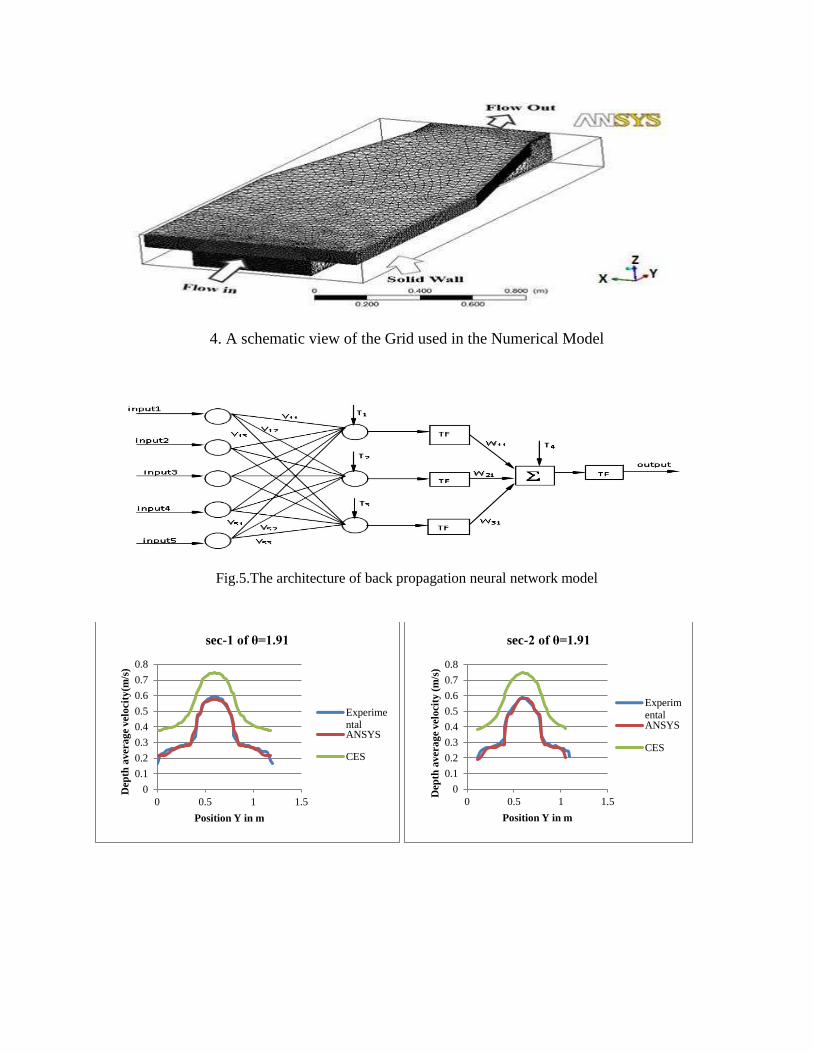
For identify the domain six different surfaces are generated. Figure 3 shows the different 236

Geometrical entities used in a non-prismatic compound channel 237

Inlet 238

Outlet 239

Free Surface 240

Side Wall 241

Channel Bottom 242

Centre line 243

244

3.2 Mesh generation 245

246

The second and very important step in numerical analysis is setting up the discretized grid 247

associated with the geometry. Construction of the mesh involves discretizing or subdividing the 248

geometry into the cells or elements at which the variables will be computed numerically. By 249

using the Cartesian co-ordinate system, the fluid flow governing equations i.e. momentum 250

equation, continuity equation are solved based on the discretization of domain. The meshing 251

divides the continuum into a finite number of nodes. Generally, one of three different methods, 252

i.e. Finite Element, Finite Volume and Finite Difference, can discretize the equations. Fluent 253

uses Finite Element (FE) based Finite Volume Method (FVM). This alternative uses the control 254

volume analysis, which is vertex-centered, i.e. the solution correlation variables are saved at the 255

nodes (vertices) of the mesh. The concept of FVM is used to convert the partial differential 256

equation into system of algebraic equation, which can be solved through closure. Two prominent 257

discretization steps involved at this stage are discretization of the computational domain and 258

discretization of the equation. The discretization of the computational domain is done through 259

mesh generation, which can be identified later through control volume constructions. However, a 260

very dense mesh of nodes causes excess computational time and memory. For CFD analysis, 261

more nodes are required in some areas of interest, such as near wall and wake regions, in order to 262

capture the large variation of fluid properties. Thus, the structure of grid lines causes further 263

unnecessary use of computer storage due to further refinement of mesh. In this study, the flow 264

domain is discretized using an unstructured grid and body-fitted coordinates. Unstructured grid is 265

used so that intricacies can be covered under the grid which is left over in structured one. The 266

detailed meshing of the flow domain is shown in Figure 4. 267

268

3.3 Solver setting 269

270

3.3.1 Setup 271

After the meshing part is completed, various inputs are given in the Setup section. VOF (volume 272

of fluid) model is the only model available for open channel flow simulation in ANSYS-273

FLUENT, which is based on the idea of volume fraction (Hirt and Nichols 1981). In this method, 274

a transport equation is solved for the volume fraction at each time step whereupon the shape of 275

the free surface is reconstructed explicitly using the distribution of the volume fraction function. 276

The “reconstruction” of the free surface can be explained more clearly through the concept of 277

water volume fraction. Free surface is defined as the cell, which takes the value of the water 278

volume fraction as non-zero while a zero value indicates that no fluid is present in the cell. The 279

value of 0.5 for the water volume fraction is indicative of the fact that free surface position is 280

detected. This method can define sharp interfaces and is robust. VOF is capable of calculating 281

time dependent solutions. Flow in an open channel is generally bound by channel from all 282

directions except for the upward free surface. To achieve a free surface zero friction interface, a 283

command called “surface_symmetry” is given in named selection. Velocity inlet for inlet and 284

pressure outlet for outlet is defined and the roughness coefficient is added to the walls for “no 285

slip” condition. Transient flow was chosen because the flow parameters were varied in time in 286

the experiment. Gravity is check marked and the value for Z-axis is given as -9.81 because 287

gravity acts downward opposite to the z-direction vector. As mentioned earlier, the turbulence 288

model was chosen as k- の model. PISO was selected for solving the pressure equation, as it is 289

generally a pressure-based segregated algorithm recommended for transient flow conditions (Issa 290

1986). Also, PISO scheme may aid in accelerating convergence for many unsteady flows. 291

Finally, solver is patched and run to apply all the settings as well as conditions mentioned above. 292

It’s just finalizing and complying the settings. The equation solved in the CFD are usually 293

iterative and starting from initial approximation, they iterate to a final result. However, these 294

iterations are terminated at some step to minimize the numerical effort. This termination are done 295

on the basis of normalized residual target which is by default is set to 10-4, which leads to loose 296

convergence target. For problems like compound channel in order to obtain more accuracy 297

residual target should be placed a value near around 10-6. Time step size was set to 0.001s and 298

number of iteration given was 1000 for better accuracy and convergence of the iteration. Time 299

step size, ∆t, is then set in the Iterate panel, ∆t must be small enough to resolve time-dependent 300

features; making sure that the convergence is reached within the number of max iterations per 301

time step. The order of magnitude of an appropriate time step size can be estimated as ratio of 302

typical cell size to the characteristic flow velocity. Time step size estimate can also be chosen so 303

that the unsteady characteristics of the flow can be resolved (e.g. flow within a known period of 304

fluctuations). To iterate without advancing in time, use zero time steps. 305

306

3.3.2 Governing Equations 307

ANSYS Fluent uses the finite volume method to solve the governing equations for a fluid. It 308

provides the capability to use different physical models such as incompressible or compressible, 309

inviscid or viscous, laminar or turbulent etc. The most practical and still the most popular 310

method of dealing with turbulence is that based on the RANS method. With this method, all 311

scales of turbulence are modelled. Several models were studied to compare the effect of 312

turbulent modeling in the converging compound channel, including the following: (1) k-Epsilon, 313

(2) k-の and (3) Large Eddy Simulation (LES) model. Here k-＼ model is used for turbulence 314

modeling. The k-の model solves the k-transport equation and a transport equation for の. The k-315

transport equation and the transport equation for の can be written (Wilcox 1988) 316

317

擢賃擢痛 髪 戟沈 擢賃擢掴日 噺 擢擢掴日 岾 塚禰蹄入 擢賃擢掴日峇 髪 鶏 伐 紅嫗倦降 (1) 318

319 擢摘擢痛 髪 戟沈 擢賃擢掴日 噺 擢擢掴日 岾 塚禰蹄狽 擢賃擢掴日峇 髪 糠 摘賃 鶏 伐 紅降態 (2) 320

321

and the eddy viscosity is given by 322

323 鉱痛 噺 倦【降 (3) 324

325

P is the turbulence kinetic energy production rate. Menter [49] as suggested the turbulence 326

equation: 327

328

P = min (P, 10紅嫗倦降) (4) 329

It represents the rate at which the energy is fed from the mean flow to each stress component. 330

The estimation of the production term can be done directly from the stress and the men flow 331

strain rate components and thus needs no modelling other than this all other terms need 332

modelling. 333

The k-の model involves five empirical constants く’, く, g, jk and jの. They have their universal 334

constant values, which have been derived on the basis of high quality data. Their values vary 335

from one turbulence model to another. For any particular turbulence model, the values of these 336

constants remain same for all simulation purposes. For standard k-の, their values are presented in 337

Table 2. 338

339

3.3.3 Boundary conditions 340

Four different types of boundary condition were considered in this study. These are (i) inlet, (ii) 341

outlet, (iii) water surface, and (iv) walls of the geometry 342

(i) Inlet 343

The velocity distribution at the upstream cross-section was taken as inlet boundary condition. At 344

the inlet, turbulence properties i.e. k (turbulence kinetic energy) and (降 turbulence dissipation 345

rate) must be specified. These were calculated as [28] 346

347 倦 噺 荊戟態 (5) 348

349 降 噺 賃迭【鉄鎮 (6) 350

351

Where I is the turbulence intensity and U is the mean value of stream-wise velocity. l is the 352

turbulence length scale 353

(ii) Outlet 354

At the outlet, the pressure condition was given as the boundary condition and pressure was fixed 355

at zero. Importance of the outflow boundary at an appropriate location can be explained through 356

the influence of the downstream condition. Thus it makes extremely imperative to put the 357

downstream end far enough to prevail the fully developed state. 358

(iii) Channel and Floodplain Boundaries 359

A no-slip boundary condition was considered at the walls. This means that the velocity 360

components should be zero at the walls. The no-slip condition is the default, and it indicates that 361

the fluid sticks to the wall and moves with the same velocity as the wall, if it is moving. The wall 362

is the most common boundary condition in bounded fluid flow problem. Setting the velocity near 363

wall as zero under no-slip condition is appropriate condition for the solid boundary. The wall 364

boundary condition in the turbulent flow is implemented and initiated by evaluating the 365

dimensionless distance ‘z+’ from the wall to the nearest boundary node. This dimensionless 366

distance is the function of the near wall node to the solid boundary, friction velocity and the 367

kinematic viscosity. The near wall treatment will depend on the position of the nearest to the 368

boundary node. If z+判 11.06 the nearest to boundary node will lie in the viscous sub-laminar 369

layer where profile is linear and very fine meshing is required. This will tend to intensify the 370

computation effort, which is being dedicated for near wall treatment. In another case where 371

z+伴11.06 the nearest boundary node will lie in the buffer layer which is the transition region 372

from viscous sublayer and the log law region. The main shortcoming of the wall function 373

approach is their dependability on the nearest node distance from the wall, which cannot be 374

overcome through refining since it does not guarantees high accuracy. Nevertheless, the problem 375

of discrepancy in the wall function approach can be subsidized through Scalable wall function 376

where limiting the z+ value to not fall below 11.06 (the intersection of linear profile and log-law) 377

is concentrated. Therefore, all mesh points are made lie outside the viscous sublayer and all fine 378

mesh discrepancies are circumvented. 379

Thus, standard wall-function, which uses log-law of the wall to compute the wall shear stress is, 380

used [50]. Fluid flows over rough surfaces are encountered in diverse situations. If the modeling 381

is a turbulent wall-bounded flow in which the wall roughness effects are considered significant, 382

it can include the wall roughness effects through the law-of-the-wall modified for roughness. 383

(iv) Free Surface 384

The water surface was defined as a plane of symmetry, which means that the normal velocity and 385

normal gradients of all variables are zero at this plane. Free surface in the present study is 386

modeled through VOF for estimating the domain for air and water (multiphase problem). 387

388

3.4 Results 389

A variety of flow characteristics can be considered in the post-processing software of CFD 390

packages. This work has been concerned with the velocity distribution and the results are 391

compared with experimental measurements. In general the user should make an attempt to 392

validate the CFD results with known data so that there can be some confidence in the solution. In 393

the case of open channel flow, the validation is most likely to take the form of a comparison 394

against physical measurements and a qualitative understanding of what features should be 395

present in the flow. As part of the analysis, the user may also wish to perform a sensitivity study 396

and vary any parameters (such as roughness here) which have a degree of uncertainty, and 397

determine what influence they have on the solution. 398

399

4. PREDICTION USING ANN 400

401

ANN is a new and rapidly growing computational technique and an alternative procedure to 402

tackle complex problems. In recent years it has been broadly used in hydraulic engineering and 403

water resources [36, 37]. It is a highly self-organized, self-adapted and self-trainable 404

approximator with high associative memory and nonlinear mapping. ANNs may consist of 405

multiple layers of nodes interconnected with other nodes in the same or different layers. Various 406

layers are referred to as the input layer, the hidden layer and the output layer. The inputs and the 407

inter-connected weights are processed by a weight summation function to produce a sum that is 408

passed to a transfer function. The output of the transfer function is the output of the node. In this 409

paper, multi-layer perception network is used. Input layer receives information from the external 410

source and passes this information to the network for processing. Hidden layer receives 411

information from the input layer and does all the information processing, and output layer 412

receives processed information from the network and sends the results out to an external 413

receptor. The input signals are modified by interconnection weight, known as weight factor Wij 414

which represents the interconnection of ith node of the first layer to the jth node of the second 415

layer. The sum of modified signals (total activation) is then modified by a sigmoidal transfer 416

function (f). Similarly output signals of hidden layer are modified by interconnection weight 417

(Wij) of kth node of output layer to the jth node of the hidden layer. The sum modified k signal is 418

then modified by a pure linear transfer function (f) and output is collected at output layer. 419

420

Let Ip = (Ip1, Ip2,…,Ipl), p=1,2,…,N be the pth pattern among N input patterns. Wji and Wkj are 421

connection weights between ith input neuron to jth hidden neuron and jth hidden neuron to kth 422

output neuron respectively. 423

Output from a neuron in the input layer is 424

425

Opi = Ipi , i=1, 2… l (7) 426

427

Output from a neuron in the hidden layer is 428

429

Opj = f (NETpj) = f (デ 激珍沈頚椎沈鎮沈退待 ), j = 1, 2. m (8) 430

431

Output from a neuron in the hidden layer is 432

433

Opk = f (NET pk) = f盤デ 激賃珍頚椎珍鎮沈退待 匪, k=1, 2. n (9) 434

435

4.1 Sigmoidal Function 436

A bounded, monotonic, non-decreasing, S Shaped function provides a graded non-linear 437

response. It includes the logistic sigmoid function 438

F(x) = 怠怠袋勅貼猫 (10) 439

Where x = input parameters taken 440

441

The architecture of back propagation neural network model, that is the l-m-n (l input neurons, m 442

hidden neurons, and n output neurons) is shown in the fig.5 443

444

4.2 Learning or training in back propagation neural network 445

Batch mode type of supervised learning has been used in the present case in which 446

interconnection weights are adjusted using delta rule algorithm after sending the entire training 447

sample to the network. During training, the predicted output is compared with the desired output 448

and the mean square error is calculated. If the mean square error is more, then a prescribed 449

limiting value, it is back propagated from output to input and weights are further modified until 450

the error or number of iteration is within a prescribed limit. 451

Mean Squared Error, Ep for pattern is defined as 452

Ep = デ 怠態 盤経椎沈 伐 頚椎沈匪態津沈退怠 (11) 453

Where Dpi is the target output, Opi is the computed output for the ith pattern. 454

Weight changes at any time t, is given by 455 ッ 激岫建岻 噺 伐券継椎岫建岻 髪 糠 抜 ッ激岫建 伐 な岻 (12) 456

n = learning rate i.e. ど 隼 券 隼 な 457 糠 = momentum coefficient i.e. ど 隼 糠 隼 な 458

4.3 Source of data 459

The data are collected from research work done in Hydraulic and Fluid Mechanics Laboratory, 460

NIT Rourkela, [44] data, available at the laboratory of University of Birmingham, Wallingford 461

and also generated data by using ANSYS-15 .The descriptions of geometrical parameters of 462

above data are mentioned in Table.3. 463

464

4.4 Selection of hydraulic parameters 465

Flow hydraulics and momentum exchange in converging compound channels are significantly 466

influenced by both geometrical and hydraulic variables, the computation become more complex 467

when the floodplain width contracted and become zero. The flow factors responsible for the 468

estimation of depth-averaged velocities are 469

(i) Converging angle denoted as し 470

(ii) Width ratio (g) i.e .ratio of width of floodplain to width of main channel 471

(iii) Aspect ratio (j) i.e. ratio of width of main channel (B) to depth of main channel (h) 472

(iv) Depth ratio (く) = (H-h)/H, where H=height of water at a particular section and, h= height of 473

water in main channel 474

(v) Relative distance (Xr) i.e of point velocity in the length wise direction of the channel)/total 475

length of the non-prismatic channel. Total five flow variables were chosen as input parameters 476

and depth-averaged velocity as output parameter. 477

478

5. RESULTS 479

480

5.1 Results of ANSYS and CES 481

482

5.1.1 Verification 483

The values of depth-averaged velocity distributions of different cross-sections of the non-484

prismatic compound channel are achieved from the numerical models like CES (Conveyance 485

Estimating System) and ANSYS then the results from the experimental data of both NITR and 486

[44] channels were compared in Figures 6-11. As illustrated in Figures 6-10, the numerical 487

model was in good agreement with experimental results but the results of the CES model have 488

some differences with experimental results. The Conveyance and Afflux Estimation System 489

(CES/AES) is a software tool for the improved estimation of flood and drainage water levels in 490

rivers, watercourses and drainage channels. The software development followed 491

recommendations by practitioners and academics in the UK Network on Conveyance in River 492

Flood Plain Systems, following the Autumn 2000 floods, that operating authorities should make 493

better use of recent improved knowledge on conveyance and related flood (or drainage) level 494

estimation. This led to a Targeted Program of Research aimed at improving conveyance 495

estimation and integration with other research on afflux at bridges and structures at high flows. 496

The CES/AES software tool aims to improve and assist with the estimation of: 497

hydraulic roughness 498

water levels (and corresponding channel and structure conveyance) 499

flow (given slope) 500

section-average and spatial velocities 501

backwater profiles upstream of a known flow-head control e.g. weir (steady) 502

afflux upstream of bridges and culverts 503

uncertainty in accuracy of input data and output 504

Conveyance Estimation System (CES) is developed by joint Agency/DEFRA research program 505

on flood defence, with contributions from the Scottish Executive and the Northern Ireland Rivers 506

Agency, HR Wallingford. CES is based Reynolds-averaged Navier-Stokes (RANS) approach as 507

the solution basis for estimation of conveyance. RANS equation of CES has been solved 508

analytically by Shiono & Knight method. In this solution the converging fluid plain effect has 509

not been considered which is reflected by the results of depth-averaged velocity and giving much 510

error However, Fluent K-の model take care of converging effect as well as interaction effect of 511

geometry of converging compound channel. 512

513

5.2 Results of ANN 514

5.2.1 Testing of Back propagation neural network 515

Determination of depth-averaged velocity distribution of compound channel with converging 516

flood plain is an important task for river engineer. Due to nonlinear relationship between the 517

dependent and independent variables any model tools to provide the accurate depth-averaged 518

velocity distribution. Numerical approach has also consumed more memory and time. So in the 519

present work the ANN has been tested. The total experimental data set is divided into training set 520

and testing set. For depth-averaged velocity calculations 32321 data are used among which 70% 521

are training data and 30% are taken as testing data. The number of layers and neurons in the 522

hidden layer are fixed through exhaustive experimentation when mean square error is minimised 523

for training data set. It is observed that minimum error is obtained for 5-7-1 architecture. So the 524

back propagation neural network (BPNN) used in this work has three layered feed forward 525

architecture. The model was run on MATLAB commercial software dealing with trial and error 526

procedure. 527

528

A regression curve is plotted between actual and predicted depth-averaged velocity of testing 529

data which are shown in figure (12) .It can be observed that data are well fitted because a high 530

degree of coefficient of determination R2 of 0.91. Figure 13 shows the error histogram plot of the 531

model. 532

533

6. ERROR ANALYSIS 534

535

To check the strength of the model, with the result from CES error analyses have been done. 536

Mean Absolute Error (MAE), the Mean Absolute Percentage Error (MAPE), Mean Squared 537

Error (MSE), the Root Mean Squared Error (RMSE) for all the converging compound channels 538

for different geometry and flow conditions have been estimated. Efficiency criterion like R2, 539

Nash-Sutcliffe efficiency (E) have also been estimated to provide more information on the 540

systematic and dynamic errors present in the model simulation. The definitions of error terms are 541

described below. The detailed results of the error analysis have been presented in table 4 .The 542

expression used to estimate errors in different forms are 543

1. Mean Absolute Error (MAE) 544

The Mean Absolute Error has been evaluated as, 545

546 警畦継 噺 怠津 デ 嵳牒日貸潮日潮日 嵳津沈 (13) 547

548

Where Pi=predicted values, Oi=observed values 549

550

2. Mean Absolute Percentage Error (MAPE) 551

Mean Absolute Percentage Error also known as Mean absolute Percentage Deviation. It was 552

usually expressed as a percentage, and was defined by the formula 553

554 警畦鶏継 噺 怠津 デ 嵳潮日貸牒日潮日 嵳津沈 (14) 555

3. Mean Squared Error (MSE) 556

Mean Squared Error measures the average of the squares of the errors. It is computed as 557 警鯨継 噺 怠津 デ 岫鶏沈 伐 頚沈岻態津沈 (15) 558

4. Root Mean Squared Error (RMSE) 559

Root Mean Squared Error or Root Mean Squared Deviation is also a measure of the differences 560

between values predicted by model or an estimator and the actually observed values. These 561

individual differences are called as residuals when the calculations are performed over the data 562

sample that is used for estimation, and are known as estimation errors when computed out 563

of the sample. The RMSE is defined as 564

565 迎警鯨継 噺 ヂ警鯨継 (16) 566

5. Coefficient of correlation R2 567

The coefficient of correlation R2 can be expressed as the squared ratio between the covariance 568

and the multiplied standard deviations of the observed and predicted values. The range of R2 lies 569

between 0 and 1.0 which describes how much of the observed dispersion is explained by the 570

prediction. A value of zero means no correlation at all whereas a value of 1 means that the 571

dispersion of the prediction is equal to that of the observation. 572

573

574

6. Nash-Sutcliffe efficiency E 575

The efficiency E proposed by Nash and Sutcliffe [51] is defined as: 576 継 噺 な 伐 デ 岫潮日貸牒日岻鉄韮日デ 岫潮日貸潮博岻鉄韮日 (17) 577

Where 頚博 represents the mean of calculated values. The range of E lies between 1.0 (perfect fit) 578

and –∞. 579

580

7. CONCLUSIONS 581

582

In this study numerical analysis for prediction of depth-averaged velocity for compound channel 583

with converging flood plain using ANN were presented. In the first part of the paper, a 3D model 584

of turbulence stream pattern in compound channel with converging flood plains were simulated 585

using a numerical model. Using experimental and numerical analysis, variation of velocity 586

components for compound channel with converging flood plains were studied. The other part of 587

this paper dealt with the prediction of the depth-averaged velocity field using ANN. In the 588

prediction part, at first, BPNN neural networks were created. Then coordinates of different points 589

were applied as input values and corresponding velocity as target outputs to create ANNs. Some 590

experimental data were used to train the ANNs and some experimental data were used to test the 591

trained ANNs based on BPNN techniques. Finally, the results of ANN and CES methods were 592

compared in sections. The main conclusions of this study are as follows: 593

594

1. ANSYS shows a good conformity with the experimental results for predicting the depth-595

averaged velocity. 596

597

2. Results of numerical model showed that the CES was not in good agreement with 598

experimental results for predicting the depth-averaged velocity. Since the one dimensional model 599

of CES is incompetent when it comes to more realistic results. 600

601

3. Results of ANNs that had been trained using BPNN indicated that the velocity field was 602

predicted with good approximation in both training and testing methods and it was concluded 603

that the proposed procedures are useful for velocity prediction in non-prismatic compound 604

channel with converging flood plain. 605

606

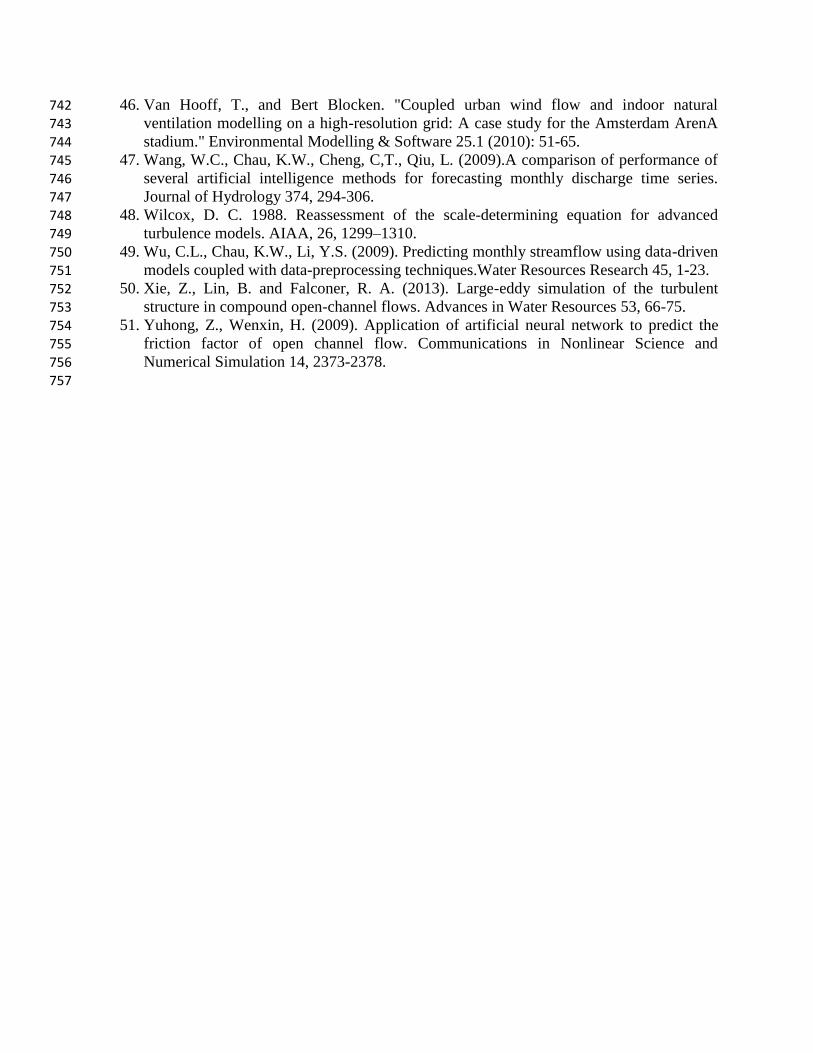
4. Different error analyses are performed to test the strength of the present ANN model. It is 607

found that MAE as 0.033,MAPE as 3.29 which less than 10%,MSE as 0.0004, RMSE as 0.02, E 608

as 0.0.95, R2 as 0.99 where as CES gave MAE as 0.2, MAPE as 20, MSE as 0.008, RMSE as 609

0.08, E as 0.75, R2 as 0.7. 610

611

5. The main advantage of ANN is the prediction of the approximate velocity at points where 612

experimental data are not available. In addition, the presented procedure can be used in 613

predicting some other properties of flow besides velocity, such as shear stresses, depth of water 614

or variations of channel bed. In addition, the presented procedure can be applied to prediction 615

and analysis of the properties of other types of channels and other structures across the flow. 616

617

Turbulence studies can also be carried out on the same guidelines indicating the turbulent 618

shearing through Reynolds stresses, secondary flow structures, and the turbulent kinetic energy, 619

which can significantly indicate the momentum exchange process and mass transfer due to 620

differential velocity due to two different stages. Overall studies consider only depth averaged 621

streamwise velocity prediction only, since the applicability of numerical modelling is 622

corroborated on the converging compound channel. Since the validation and error analysis shows 623

an undisputable results, which suggestively indicate the application of the numerical method for 624

further studies such as turbulence studies. 625

626

8. ACKNOWLEDGEMENTS 627

628

The author wish to acknowledge the support from the Institute and the UGC UKIERI Research 629

project (ref no UGC-2013 14/017) by the second authors for carrying out the research work in 630

the Hydraulics Laboratory at National Institute of Technology, Rourkela. 631

632

633

634

9. REFERENCES 635

636

1. Abdeen, M. A. M. (2008). Predicting the impact of vegetations in open channels with 637

different distributaries’ operations on water surface profile using artificial neural 638

networks. Journal of Mechanical Science and Technology, 22, 1830–1842. 639

2. Bhattacharya,B. & Solomatine, D. P. (2005). Neural networks and M5 model trees in 640

modelling water level–discharge relationship. Neurocomputing, 63, 381–396. 641

3. Bilgil, A., Altun, H. (2008). Investigation of flow resistance in smooth open channels 642

using artificial neural networks. Flow Measurement and Instrumentation 19, 404-408. 643

4. Cater, J. E. and Williams, J. J. R. (2008). Large eddy simulation of a long asymmetric 644

compound open channel. 645

5. Cheng, C.T., Ou, C.P., Chau, K.W. (2002). Combining a fuzzy optimal model with 646

agenetic algorithm to solve multi-objective rainfall–runoff model calibration. Journal of 647

Hydrology 268, 72–86. 648

6. Cokljat, D. (1993). Turbulence Models for Non-circular Ducts and Channels. PhD 649

Thesis, City University London. 650

7. Ervine, D. A., Koopaei K. B. and Sellin R. H. J. (2000). Two Dimensional Solution for 651

Straight and Meandering Over-bank Flows. J. Hydraul. Eng., ASCE, 126 (9), 653-669. 652

8. Filonovich MS, Azevedo R, Rojas-Solórzano L, Leal, JB (2013). Credibility Analysis of 653

Computational Fluid Dynamic Simulations for Compound Channel Flow. Journal of 654

Hydroinformatics 15(3), 926-938. 655

9. Gandhi, B.K., Verma, H.K., Abraham, B.(2010). Investigation of Flow Profile in Open 656

Channels using CFD, 8th Intl Conference on Hydraulic Efficiency Measurement, 243-657

251. 658

10. Ghosh, S., and Jena, S.B. (1971). Boundary shear stress distribution in open channel 659

compound. Proc. Inst. Civil Eng. 49, 417–430. 660

11. Ghosh, S., Pratihar, D.K., Maiti, B., Das, P.K. (2010). Optimum design of a two step 661

planar diffuser: A hybrid approach. Engineering Applications of Computational Fluid 662

Mechanics 4(3), 415-424. 663

12. Hodges, B. R., & Street, R. L. (1999). On simulation of turbulent nonlinear free-surface 664

flows. J. Comp. Phys. 151, 425–457. 665

13. Hodskinson, A., and R. Ferguson,(1998). Numerical modelling of separated flow in river 666

bends: model testing and experimental investigation of geometric controls on the extent 667

of flow separation at the concave bank. Hydrological Processes, 12, 1323-1338. 668

14. Hodskinson, A.,(1996). Computational fluid dynamics as a tool for investigating 669

separated flow in river bends. Earth Surface Processes and Landforms,21, 993-1000. 670

15. Hsu, T. Y., Grega, L. M., Leighton, R. I. and Wei, T. (2000). Turbulent kinetic energy 671

transport in a corner formed by a solid wall and a free surface. J. Fluid Mech. 410, 343-672

366. 673

16. Issa, R. I. (1986). Solution of the implicitly discretised fluid flow equations by operator-674

splitting. Journal of computational physics, 62(1), 40-65. 675

17. J. Hydraulic Research 46 (4), 445-453. 676

18. Jain, S. K. (2008).Development of integrated discharge and sediment rating relation using 677

a compound neural network. Journal of Hydrologic Engineering 13, 124–131. 678

19. Kara, S., Stoesser, T. and Sturm, T. W. (2012). Turbulence statistics in compound 679

channels with deep and shallow overbank flows. J. Hydraulic Research 50 (5), 482-493. 680

20. Kawahara,Y., & Tamai, N. (1988). Numerical calculation of turbulent flows in 681

compound channels with an algebraic stress turbulence model. In: Proc. 3rd Symp. 682

Refined Flow Modeling and Turbulence Measurements, Tokyo, Japan, pp. 9–17. 683

21. Khatua K.K, Patra K C, Mohanty, P.K. (2012). Stage Discharge Prediction for Straight 684

and Smooth Compound Channels with Wide Floodplains. J. Hydraul. Eng., ASCE, 138 685

(1), 93-99. 686

22. Khatua, K.K., Patra, K.C. (2008). Boundary Shear Stress Distribution in Compound 687

Open Channel Flow. J. Hydraul. Eng., ISH, 12 (3), 39-55. 688

23. Knight, D. W., Wright, N. G. and Morvan, H. P. (2005) .Guidelines for applying 689

commercial CFD software 690

24. Krishnappan,B. G., and Lau, Y. L. 1986. Turbulence modelling of flood plain flows. J. 691

Hydraulic Eng., ASCE, 112(4), 251-266. 692

25. Lane S. N., Bradbrook, K. F., Richards, K. S., Biron, P. A. & Roy, A. G. (1999). The 693

application of computational fluid dynamics to natural river channels: three-dimensional 694

versus two dimensional approaches. Geomorphology 29, 1–20. 695

26. Lin, J.Y., Cheng, C.T., Chau, K.W. (2006). Using support vector machines for long-term 696

discharge prediction. Hydrological Sciences Journal 51(4): 599-612. 697

27. Menter, F. R. (1994) .Two-equation eddy-viscosity turbulence models for engineering 698

applications. AIAA, 32 (8), 1598 – 1605. 699

28. Morvan, H. P.(2001). Three-dimensional Simulation of River Flood Flows. PhD 700

Thesis,University of Glasgow, Glasgow. 701

29. Muzzammil, M. (2008). Application of neural networks to scour depth prediction at the 702

bridge abutments. Engineering Applications of Computational Fluid Mechanics 2(1), 30-703

40. 704

30. Myers,W. R. C., and Elsawy (1975). Boundary Shear in Channel with Floodplain. J. 705

Hydraul. Eng., ASCE, 101(HY7), 933-946. 706

31. Nakayama, A. & Yokojima, S. (2002). LES of open-channel flow with free-surface 707

fluctuations. In: Proc. Hydraul. Eng. JSCE. 46, 373–378. 708

32. NASH, J. E., SUTCLIFFE, J. V.(1970). River flow forecasting through conceptual 709

models, Part I. A discussion of principles.J. Hydrol. 10, 282–290. 710

33. Pan, Y., & Banerjee, S. (1995). Numerical investigation of free-surface turbulence in 711

open-channel flows. Phys. Fluids ,113 (7),1649–1664. 712

34. Rezaei, B.(2006). Overbank flow in compound channels with prismatic and non-713

prismatic floodplains. PhD Thesis. Univ. of Birmingham. U.K. 714

35. Rhodes, D. G., and Knight, D. W. (1994). Distribution of Shear Force on Boundary of 715

Smooth Rectangular Duct. Journal of Hydralic Engg., 120-7, 787– 807. 716

36. Safikhani, H., Khalkhali, A., Farajpoor, M. (2011). Pareto Based Multi-Objective 717

Optimization of Centrifugal Pumps Using CFD, Neural Networks and Genetic 718

Algorithms. Engineering Applications of Computational Fluid Mechanics 5(1), 37-48. 719

37. Sahu, M., Khatua, K. K. & Mahapatra, S. S. (2011). A neural network approach for 720

prediction of discharge in straight compound open channel flow. Flow Measurement and 721

Instrumentation, 22, 438–446. 722

38. Shiono, K., Knight, D. W. (1988). Refined Modelling and Turbulance Measurements. 723

Proceedings of 3rd International Symposium, IAHR, Tokyo, Japan, July, 26-28. 724

39. Sinha, S. K., Sotiropoulos, F. & Odgaard, A. J.(1998). Three dimensional numerical 725

model for flow through natural rivers.J. Hydraul. Eng. 124(1), 13–24. 726

40. Spalding, D. B. (1980) .Genmix: a general computer program for two-dimensional 727

parabolic phenomena, Pergamon Press, Oxford. 728

41. Speziale, C. G., Sarkar, S. and Gatski, T. B. (1991) .Modelling the pressure-strain 729

correlation of turbulence: an invariant dynamical systems approach. J. Fluid Mech. 277, 730

245-272. 731

42. Thomas, T. G. and Williams, J. J. R. (1995a). Large eddy simulation of turbulent flow in 732

an asymmetric compound channel. J. Hydraulic Research 33 (1), 27-41. 733

43. to open channel flow. Report based on the research work conducted under EPSRC Grants 734

GR/R43716/01 and GR/R43723/01. 735

44. Unal, B., Mamak, M., Seckin, G. & Cobaner, M. (2010). Comparison of an ANN 736

approach with 1-D and 2-D methods for estimating discharge capacity of straight 737

compound channels. Advances in Engineering Software, 41, 120–129. 738

45. Van Hooff, T., & Blocken, B. (2010). Coupled urban wind flow and indoor natural 739

ventilation modelling on a high-resolution grid: A case study for the Amsterdam ArenA 740

stadium. Environmental Modelling & Software, 25(1), 51-65. 741

46. Van Hooff, T., and Bert Blocken. "Coupled urban wind flow and indoor natural 742

ventilation modelling on a high-resolution grid: A case study for the Amsterdam ArenA 743

stadium." Environmental Modelling & Software 25.1 (2010): 51-65. 744

47. Wang, W.C., Chau, K.W., Cheng, C,T., Qiu, L. (2009).A comparison of performance of 745

several artificial intelligence methods for forecasting monthly discharge time series. 746

Journal of Hydrology 374, 294-306. 747

48. Wilcox, D. C. 1988. Reassessment of the scale-determining equation for advanced 748

turbulence models. AIAA, 26, 1299–1310. 749

49. Wu, C.L., Chau, K.W., Li, Y.S. (2009). Predicting monthly streamflow using data-driven 750

models coupled with data-preprocessing techniques.Water Resources Research 45, 1-23. 751

50. Xie, Z., Lin, B. and Falconer, R. A. (2013). Large-eddy simulation of the turbulent 752

structure in compound open-channel flows. Advances in Water Resources 53, 66-75. 753

51. Yuhong, Z., Wenxin, H. (2009). Application of artificial neural network to predict the 754

friction factor of open channel flow. Communications in Nonlinear Science and 755

Numerical Simulation 14, 2373-2378. 756

757

Table1.Hydraulic parameters for the experimental channel data

Sl. No Item Description Converging Compound Channel 1 Geometry of main channel Rectangular

2 Geometry of flood plain Converging

3 Main channel width (b) 0.5m

4 Bank full depth of main channel 0.1m

5 Top width of compound channel (B1) before convergence 0.9m

6 Top width of compound channel (B2) after convergence 0.5m

7 Converging length of the channels 0.84m, 1.26, 2.26m

8 Slope of the channel 0.0011

9 Angle of convergence of flood plain (楢) 12.38,9, 5

10 Position of experimental section 1 start of the converging part

11 Position of experimental section 2 Middle of converging part

12 Position of experimental section end of converging part.

Table 2. Values of the constants in the k- の model (Wilcox 1988)

く’ く g jk jの 0.09 0.075 5/9 2 2

Table 3.Input and output data used for the present analysis

Sl.No Converging

angles Flood plain

type Converging

Length 1 1.91 Convergent 6m 2 3.81 Convergent 6m 3 11.31 Convergent 2m 4 5 Convergent 2.26m 5 9 Convergent 1.28m 6 12.38 Convergent 0.84m 8 2.5 Convergent 4.58 9 3 Convergent 3.82 10 4 Convergent 2.86 11 7 Convergent 1.64 12 10 Convergent 1.15 13 14 Convergent 0.8 14 15 Convergent 0.77

15 17 Convergent 0.68 16 20 Convergent 0.58

Table 4 Different Error Analysis

ANN CES

MSE 0.0004 0.008

RMSE 0.02 0.08

MAE 0.033 0.2

MAPE 3.29 20

E 0.95 0.70

R2 0.99 0.75

Figure 1(a). Plan view of Experimental Setup

Figure 1(b). Plan view of different test reaches with cross-sectional dimensions of non-prismatic

compound channel from both NITR & Rezaei (2006) channels

Figure 1(c). Typical grid showing the arrangement of velocity measurement points at the test

sections (1-1,2-2,3-3,4-4 &5-5)

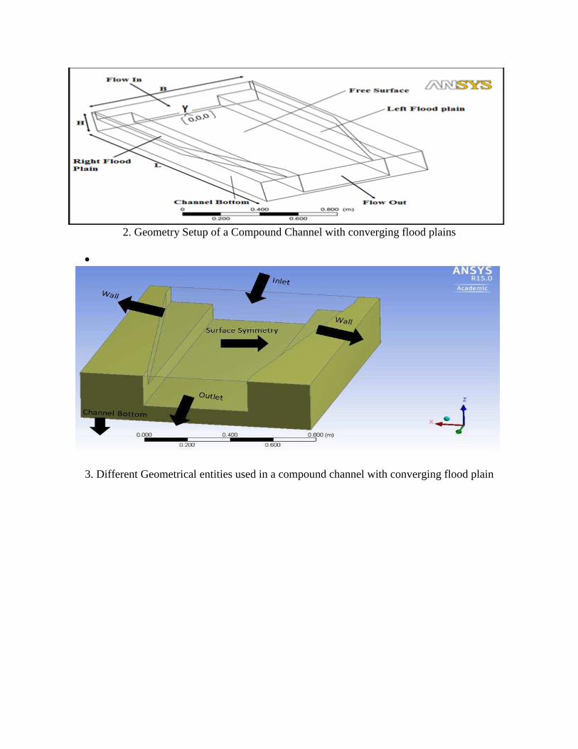
2. Geometry Setup of a Compound Channel with converging flood plains

3. Different Geometrical entities used in a compound channel with converging flood plain

4. A schematic view of the Grid used in the Numerical Model

Fig.5.The architecture of back propagation neural network model

0

0.1

0.2

0.3

0.4

0.5

0.6

0.7

0.8

0 0.5 1 1.5

Dep

th a

vera

ge v

eloc

ity(

m/s

)

Position Y in m

sec-1 of し=1.91

ExperimentalANSYS

CES

0

0.1

0.2

0.3

0.4

0.5

0.6

0.7

0.8

0 0.5 1 1.5

Dep

th a

vera

ge v

eloc

ity

(m/s

)

Position Y in m

sec-2 of し=1.91

ExperimentalANSYS

CES

Figure 6 (a) , (b) , (c) Depth-averaged velocity of Sec 1, Sec 2 , Sec 3 of し=1.910

Figure 7 (a) , (b) , (c) Depth-averaged velocity of Sec 1, Sec 2 , Sec 3 of し=3.810

0.00.10.20.30.40.50.60.70.8

0 0.5 1 1.5D

epth

ave

rage

vel

ocit

y(m

/s)

Position Y in m

sec-3 of し=1.91

ExperimentalANSYS

CES

0

0.1

0.2

0.3

0.4

0.5

0.6

0.7

0.8

0 0.5 1 1.5

Dep

th a

vera

ge v

eloc

ity(

m/s

)

Position Y in m

sec-1 of し=3.81

Experimental

ANSYS

CES

0

0.1

0.2

0.3

0.4

0.5

0.6

0.7

0.8

0 0.5 1 1.5

Dep

th a

vera

ge v

eloc

ity(

m/s

)

Position Y in m

sec-2 of し=3.81

Experimental

ANSYS

CES

0

0.1

0.2

0.3

0.4

0.5

0.6

0.7

0.8

0 0.5 1

Dep

th a

vera

ge v

eloc

ity(

m/s

)

Position Y in m

sec-3 of し=3.81

ExperimentalANSYS

CES

Figure 8 (a) , (b) , (c) Depth-averaged velocity of Sec 1, Sec 2 , Sec 3 of し=11.310

0.0

0.1

0.2

0.3

0.4

0.5

0.6

0.7

0.8

0.0 0.5 1.0 1.5

Dep

th a

vera

ge v

eloc

ity(

m/s

)

Position Y in m

sec-1 of し=11.31

Experimental

ANSYS

CES

0

0.1

0.2

0.3

0.4

0.5

0.6

0.7

0.8

0 0.5 1 1.5

Dep

th a

vera

ge v

eloc

ity(

m/s

)

Position Y in m

sec-2 of し=11.31

Experimental

ANSYS

CES

0

0.1

0.2

0.3

0.4

0.5

0.6

0.7

0.8

0 0.5 1

Dep

th a

vera

ge v

eloc

ity(

m/s

)

Position Y in m

sec-3 of し=11.31

ExperimentalANSYS

CES

0

0.1

0.2

0.3

0.4

0.5

0.6

0.7

0.8

0.9

0 0.5 1

Dep

th a

vera

ge v

eloc

ity(

m/s

)

Position Y in m

sec-1 of し=5

Experimental

ANSYS

CES

0

0.1

0.2

0.3

0.4

0.5

0.6

0.7

0.8

0.9

0 0.5 1

Dep

th a

vera

ge v

eloc

ity(

m/s

)

Position Y in m

sec-2 of し=5

Experimental

ANSYS

CES

Figure 9 (a) , (b) , (c) Depth-averaged velocity of Sec 1, Sec 2 , Sec 3 of し =50

Figure 10 (a) , (b) , (c) Depth-averaged velocity of Sec 1, Sec 2 , Sec 3 of し =90

0

0.2

0.4

0.6

0.8

1

1.2

0 0.5 1D

epth

ave

rage

vel

ocit

y(m

/s)

Position Y in m

sec-3 of し=5

ExperimentalANSYS

CES

0

0.1

0.2

0.3

0.4

0.5

0.6

0.7

0.8

0 0.5 1

Dep

th a

vera

ge v

eloc

ity(

m/s

)

Position Y in m

sec-1 of し=9

ExperimentalANSYS

CES

0

0.1

0.2

0.3

0.4

0.5

0.6

0.7

0.8

0 0.5 1

Dep

th a

vera

ge v

eloc

ity(

m/s

)

Position Y in m

sec-2 of し=9

ExperimentalANSYS

CES

0

0.2

0.4

0.6

0.8

1

1.2

0 0.5 1

Dep

th a

vera

ge v

eloc

ity(

m/s

)

Position Y in m

sec-3 of し=9

Experimental

ANSYS

CES

Figure 11 (a) , (b) , (c) Depth-averaged velocity of Sec 1, Sec 2 , Sec 3 of し =12.380

Fig 13 Correlation plot of actual depth-averaged velocity and predicted depth-averaged velocity

0

0.1

0.2

0.3

0.4

0.5

0.6

0.7

0.8

0.9

0 0.5 1

Dep

th a

vera

ge v

eloc

ity

(m/s

)

Position Y in m

sec-1 of し=12.38

experimentalANSYS

CES

0

0.1

0.2

0.3

0.4

0.5

0.6

0.7

0.8

0.9

0 0.5 1

Dep

th a

vera

ge v

eloc

ity(

m/s

)

Position Y in m

sec-2 of し=12.38

CES

ANSYS

Experimental

0.74

0.76

0.78

0.8

0.82

0.84

0.86

0.88

0 0.5 1

Dep

th a

vera

ge v

eloc

ity(

m/s

)

Position Y in m

sec-3 of し=12.38

Experimental

ANSYS

CES

Fig 14 Error Histogram