NUMERICAL MODELING FOR MULTIPHASE INCOMPRESSIBLE FLOW … publications/2005... · numerical...

NUMERICAL MODELING FOR MULTIPHASEINCOMPRESSIBLE FLOW WITH PHASE CHANGE

Xiao-Yong Luo, Ming-Jiu Ni, Alice Ying, and M. A. AbdouMechanical & Aerospace Engineering Department, University of California,Los Angeles, Los Angeles, California, USA

A general formula for the second-order projection method combined with the level set

method is developed to simulate unsteady, incompressible multifluid flow with phase change.

A subcell conception is introduced in a modified mass transfer model to accurately calculate

the mass transfer across the interface. The third-order essentially nonoscillatory (ENO)

scheme and second-order semi-implicit Crank-Nicholson scheme is employed to update

the convective and diffusion terms, respectively. The projection method has second-order

temporal accuracy for variable-density unsteady incompressible flows as well. The level

set approach is employed to implicitly capture the interface for multiphase flows. A con-

tinuum surface force (CSF) tension model is used in the present cases. Phase change

and dynamics associated with single bubble and multibubbles in two and three dimensions

during nucleate boiling are studied numerically via the present modeling. The numerical

results show that this method can handle complex deformation of the interface and account

for the effect of liquid–vapor phase change.

1. INTRODUCTION

The heat transfer and incompressible flow processes associated with phase-change phenomena are typically among the complex transport circumstancesencountered in engineering applications, such as power and refrigeration cycles, pet-roleum and chemical processing, thermal control of aircraft avionics and spacecraftenvironments, and operating circumstances of nuclear power plant design. Theseprocesses may have complexities including nonlinearities, time-varying behavior,dynamic interaction between the phases, and motion of the interface. Theoreticaland experimental studies have laid the necessary groundwork for the phase change,but it is clear that computational modeling can provide accurate predictions ofphysical phenomena with complex interactions among many effects such as fluidflow, surface tension, and heat and mass transfer with phase change. However, accu-rate numerical investigation to predict the associated heat and mass transfer hasoften proved to be a formidable task. Computations of this problem are still farbehind what is possible for multifluid flows without phase change. Typical numerical

Received 31 March 2005; accepted 21 May 2005.

The authors would like to thank Prof. S. Osher for fruitful discussion. This work is supported by

the U.S. Department of Energy under Grant DE-FG03-86ER52123.

Address correspondence to Xiao-Yong Luo, UCLA MAE Department, 44-136 Engineering IV,

Los Angeles, CA 90095-1597, USA. E-mail: [email protected]

425

Numerical Heat Transfer, Part B, 48: 425–444, 2005

Copyright # Taylor & Francis Inc.

ISSN: 1040-7790 print=1521-0626 online

DOI: 10.1080/10407790500274364

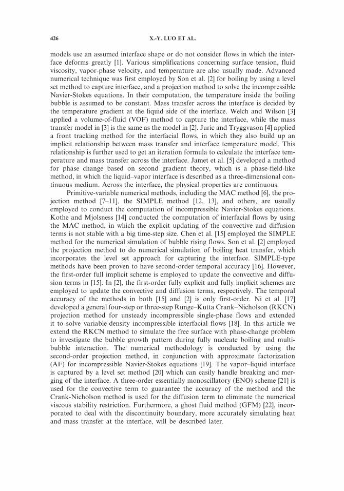
models use an assumed interface shape or do not consider flows in which the inter-face deforms greatly [1]. Various simplifications concerning surface tension, fluidviscosity, vapor-phase velocity, and temperature are also usually made. Advancednumerical technique was first employed by Son et al. [2] for boiling by using a levelset method to capture interface, and a projection method to solve the incompressibleNavier-Stokes equations. In their computation, the temperature inside the boilingbubble is assumed to be constant. Mass transfer across the interface is decided bythe temperature gradient at the liquid side of the interface. Welch and Wilson [3]applied a volume-of-fluid (VOF) method to capture the interface, while the masstransfer model in [3] is the same as the model in [2]. Juric and Tryggvason [4] applieda front tracking method for the interfacial flows, in which they also build up animplicit relationship between mass transfer and interface temperature model. Thisrelationship is further used to get an iteration formula to calculate the interface tem-perature and mass transfer across the interface. Jamet et al. [5] developed a methodfor phase change based on second gradient theory, which is a phase-field-likemethod, in which the liquid–vapor interface is described as a three-dimensional con-tinuous medium. Across the interface, the physical properties are continuous.

Primitive-variable numerical methods, including the MAC method [6], the pro-jection method [7–11], the SIMPLE method [12, 13], and others, are usuallyemployed to conduct the computation of incompressible Navier-Stokes equations.Kothe and Mjolsness [14] conducted the computation of interfacial flows by usingthe MAC method, in which the explicit updating of the convective and diffusionterms is not stable with a big time-step size. Chen et al. [15] employed the SIMPLEmethod for the numerical simulation of bubble rising flows. Son et al. [2] employedthe projection method to do numerical simulation of boiling heat transfer, whichincorporates the level set approach for capturing the interface. SIMPLE-typemethods have been proven to have second-order temporal accuracy [16]. However,the first-order full implicit scheme is employed to update the convective and diffu-sion terms in [15]. In [2], the first-order fully explicit and fully implicit schemes areemployed to update the convective and diffusion terms, respectively. The temporalaccuracy of the methods in both [15] and [2] is only first-order. Ni et al. [17]developed a general four-step or three-step Runge–Kutta Crank–Nicholson (RKCN)projection method for unsteady incompressible single-phase flows and extendedit to solve variable-density incompressible interfacial flows [18]. In this article weextend the RKCN method to simulate the free surface with phase-change problemto investigate the bubble growth pattern during fully nucleate boiling and multi-bubble interaction. The numerical methodology is conducted by using thesecond-order projection method, in conjunction with approximate factorization(AF) for incompressible Navier-Stokes equations [19]. The vapor–liquid interfaceis captured by a level set method [20] which can easily handle breaking and mer-ging of the interface. A three-order essentially monoscillatory (ENO) scheme [21] isused for the convective term to guarantee the accuracy of the method and theCrank-Nicholson method is used for the diffusion term to eliminate the numericalviscous stability restriction. Furthermore, a ghost fluid method (GFM) [22], incor-porated to deal with the discontinuity boundary, more accurately simulating heatand mass transfer at the interface, will be described later.

426 X.-Y. LUO ET AL.

Employing the variable-density projection method and the level set method tosimulate immiscible interfacial flows with phase change is the main subject of thisarticle. The physical models, a modified mass transfer model, and numerical algo-rithms are presented in Section 2. The broken-dam validation case is presented inSection 3. 2-D single-bubble growth pattern during nucleate boiling, 2-D multibub-ble dynamic interaction during nucleate boiling, and 3-D single-bubble nucleateboiling are studied numerically in Section 4. Conclusions are presented in Section 5.

2. PHYSICAL MODELS AND NUMERICAL ALGORITHMS

2.1. Governing Equations

For incompressible multiphase flows with phase change, the governing equa-tions can be written as

r � u ¼ Ja

Pe

eKKeqq2 ð½rT �C � reqqÞ" #ð1Þ

quqt

þr � ðuuÞ ¼ � 1eqqrpþ 1

Fr� Gr

Re2T

� �g þ 1eqq Re

r � ðemmruÞ

þ 1eqq Rer � ðemmruÞT þ kð/Þdð/Þr/eqq We

ð2Þ

qTqt

þ u � rT ¼ 1eqqeCCp

1

Pe½r � ðeKKrTÞ� ð3Þ

where

½rT �C ¼ ðrTÞliquid � ðrTÞgas ð4Þ

with dimensionless groups of Reynolds, Froude, Weber, Jacob, Peclet, and Grashofnumbers,

Re ¼ qlUL

mlFr ¼ U2

gLWe ¼ qlU

2L

rJa ¼ CplðTw � TsatÞ

hfg

Pe ¼ qlULCpl

KlGr ¼ g0L

3q2l blðTw � TsÞm2l

Here U and L are characteristic velocity and length, respectively; r is the surfacetension coefficient; emm ¼ m=ml ; eqq ¼ q=ql ; eKK ¼ K=Kl ; and fCpCp ¼ Cp=Cpl are the dimen-sionless viscosity, density, thermal conductivity, and specific heat. / is the level setfunction, k is the front curvature of the interface, and d is the smeared-out Diracdelta function. A continuum surface force (CSF) model [23, 24] is used to reformu-late the surface tension as a volume force.

MULTIPHASE INCOMPRESSIBLE FLOW WITH PHASE CHANGE 427

2.2. Level Set Method

The level set method [20] is employed to capture the interface implicitly byintroducing a smooth level set function /, with the zero level set as the interface,positive value outside the interface, and negative value inside the interface. Considerthe following interface evolution equation:

q/qt

þ u � r/ ¼ 0 ð5Þ

which will evolve the zero level of / ¼ 0 exactly as the actual interface moves. Thecorresponding physical variants can be expressed as

eqqnð/Þ ¼ kq þ ð1� kqÞHnð/Þ ð6Þ

emmnð/Þ ¼ km þ ð1� kmÞHnð/Þ ð7Þ

where kq ¼ qg=ql and km ¼ mg=ml . H is the smeared-out Heaviside function definedby

Hð/Þ ¼

0 / < �e

1

2þ /2e

þ 1

2psin

p/e

� ��e � / � e

1 / < e

8>>>><>>>>: ð8Þ

where e is a tunable parameter that determines the size of the bandwidth of numeri-cal smearing. A typical good value is e ¼ 1:5Dx; see Figure 1.

Since / will generally drift away from its initialized value as the signed distancewhile Eq. (5) will move the level set / ¼ 0 with the correct velocity, a reinitializationapproach based on solving the hyperbolic partial differential equation is presented in[25, 26]. The reinitialization equation is

/t ¼ Lð/0;/Þ ¼ Seð/0Þð1� jr/jÞ ð9Þ

/t ¼ Lð/0;/Þ þ kf ð/Þ ð10Þ

Figure 1. Smoothing of the Heaviside function.


where k is a local constraint and function of t only, determined by

k ¼�RX H 0ð/ÞLð/0;/ÞRX H 0ð/Þf ð/Þ ð11Þ

where

f ð/Þ ¼ H 0ð/Þjr/j ð12Þ

2.3. Variable-Density RKCN Projection Method

Ni et al. [17] developed a general four-step or three-step RKCN projectionmethod for unsteady incompressible single-phase flows and extended it to solvevariable-density incompressible interfacial flows [18]. In this article we extend theRKCN method to simulate the interfacial phase change with heat and mass transfer.The variable-density RKCN projection method for phase change can be expressed as

Amuum ¼ rm � amrpm�1 þ bmrpm�2

eqqnþ1=2ð13Þ

e~uu~uu m¼ uum þ Dt � a

mrpm�1 þ bmrpm�2

eqqnþ1=2ð14Þ

amr � rpmeqqnþ1=2

!¼ 1

Dtr � ~uum � bmr � rpm�1

eqqnþ1=2

!� 1

Dtr � um

� �ð15Þ

um ¼ ~uum � Dt � amrpm þ bmrpm�1

eqqnþ1=2ð16Þ

/mþ1 ¼ /m � Dt amþ1um � r/m þ bmþ1um�1 � r/m�1� �

ð17Þ

where

Am ¼ 1

DtI � Dt � cmeqqnþ1=2 Re

r � emmnþ1=2r� �" #

ð18Þ

rm ¼ 1

DtI � Dt � cmeqqnþ1=2 Re

r � mnþ1=2r� �" #

um�1 � am½S�m�1 � bm½S�m�2 ð19Þ

S ¼ 1eqqRer � emmnþ1=2ðruÞTh i

� 1

Fr� Gr

Re2T

� �gi �

kð/Þdð/Þr/eqqWeð20Þ


and

am ¼ 8

15;5

12;3

4

� �bm ¼ 0;� 17

60;� 5

12

� �cm ¼ 4

15;1

15;1

6

� �are coefficients of the third-order Runge-Kutta method. The velocity componentsand pressure in the intermediate velocities equation at the first substep areu�1 ¼ 0; p�1 ¼ 0 ðm� 2 ¼ �1Þ; andu0 ¼ un; p0 ¼ pn ðm� 1 ¼ 0Þ. At the third stepthey are u3 ¼ un þ 1 and p3 ¼ pnþ1, which are the updated velocities and pressurefor the next time level, nþ 1. The density, viscosity, and temperature are updatedusing /nþ1, which will be eqqnþ1=2, emmnþ1=2, and Tnþ1=2 at the next time step.

In the above variable-density RKCN projection method, the Crank-Nicholsonimplicit technique is employed to update the diffusion term for stability, and the low-storage three-stage Runge-Kutta technique is employed to update the convectiveterm for simplicity and stability. The projection method also has second-ordertemporal accuracy for variable-density unsteady incompressible flows. The diffusionterm can be spatially discretized using standard central difference schemes. Theconvective term in the momentum equation can be conveniently updated using thethird-order ENO scheme [21].

2.4. A Modified Mass Transfer Model

Mass transfer during the phase-change process is associated with the tempera-ture and density gradient near the interface, as we can see from the governing equa-tion (1). Son et al. [2] simplify it by assuming the gas side is always at saturationtemperature, so that only the temperature gradient on the liquid side is accountedfor in the mass transfer. The mass continuity and energy balance at the interface withevaporation are expressed as

m ¼ eqqðuint �~uuÞ ¼ekkrT

hfgð21Þ

Assuming that the interface is advected the same way as the level set function, thecontinuity equation can be rewritten as

r � u ¼ meqq2 � reqq ¼ekkrT

hfgeqq2 � reqq ð22Þ

with its dimensionless form

r � u ¼ Ja

Pe

krTeqq2 !

� reqq ð23Þ

This simplified model is physically pretty accurate when simulating nucleate boilingphenomena. However, the following discretization formula,

qTqx

� �across interface

¼ Tiþ1 � TI

Dxð24Þ


for the calculation of the temperature gradient will cause great error when dealingwith complex heat and mass transfer conditions, since the mass transfer is dependenton the difference of the temperature gradients on both sides of the phase interface.Unfortunately, the numerical results of [2] and [3] are acquired based on the model ofEqs. (23) and (24). For the VOF method [27], it is not so convenient to accuratelydiscretize the gradients on both sides of the free interface, since the volume fractionis discontinuous. However, for the level set method, it will be shown that we canaccurately discretize the temperature gradient very conveniently, since the level setfunction is a distance function from the front interface. In this article, we modify thismass transfer model by introducing a subcell concept to accurately calculate the tem-perature gradient on both sides in the gas–liquid phase-change region. The modifiedmass transfer model greatly improves the numerical results and is a general modelfor liquid–gas phase-change heat and mass transfer.

Since the interface usually has a fairly complex shape, the level set represen-tation of the interface is used in this work. Assuming the interface lies between thenodes i and iþ 1, the temperature at these nodes are Ti and Tiþ 1, respectively (seeFigure 2).

Taking the subcell location of the interface into account allows us to discretizethe temperature gradient more accurately. Suppose that /i � 0 and /iþ1 > 0. Definea h function to estimate the subcell interface location:

h ¼ j/ijj/ij þ j/iþ1j

ð25Þ

The interface splits this cell into two pieces of size hDx on the left and sizeð1� hÞDx on the right. Denoting the temperature value at this subcell interfacelocation by Ti, which is given by the physical properties, and discretize the tempera-ture gradient near the interface as

qTqx

� �liquid

¼ Tiþ1 � TI

ð1� hÞDxqTqx

� �gas

¼ TI � Ti

hDxð26Þ

For the Y and Z normal directions, the procedure is the same so that we canget all three values of the temperature gradient near the interface. Considering the

Figure 2. Phase interface location.


mass continuity and energy balance at the interface with phase change, we canmodify Eq. (23) as Eq. (1),

r � u ¼ Ja

Pe

eKKeqq2 ð½rT �C � reqqÞ" #ð1Þ

where

½rT �C ¼ ðrTÞliquid � ðrTÞgas ð4Þ

Once the first derivative of the temperature has been computed, the secondderivative of the temperature across the interface can be computed as follows. Wedefine

ðKTxÞiþ1=2 ¼ K� TI � Ti

hDx

� �ð27Þ

and

ðKTxÞi�1=2 ¼ K� Ti � Ti�1

hDx

� �ð28Þ

arriving at

qqx

ðKTxÞi ¼ðKTxÞiþ1=2 � ðKTxÞi�1=2

Dxð29Þ

The formula of Eqs. (1) and (4) coupling with the numerical models of Eqs. (26)–(29)will be called the subcell model, and the original model of Eqs. (23) and (24) will becalled the old model later in this article.

3. NUMERICAL SIMULATION OF VALIDATION CASES

The broken dam problem is calculated to further validate the code by compar-ing the numerical result with the experimental data. An 81� 41 uniform Cartesiangrid is used with initial water column height-to-width ratio of 2. qwater=qback ¼ 1; 000; mwater=mback ¼ 1; 000; and Re ¼ 1; 000. At the outlet boundary, theNeumann boundary condition is set for velocities. At all other boundaries, slip wallboundary conditions are applied for the velocities. Figure 3 illustrates the freesurface profiles between time ¼ 0.2 and time ¼ 3.0 with time interval of 0.2. Thewater surface evolves in a smooth shape and no oscillation occurs at the interfacenear the solid wall.

Figure 4a shows the history of the waterfront moving along the ground surface( y ¼ 0), and Figure 4b shows the transient height of the wetted wall along thevertical surface (x ¼ 0). The error bar in Figure 4a shows the interface height in thiscalculation. The experimental results from Martin and Moyce (1952) are also shownin Figure 4. The numerical results match the experimental data well.


4. NUMERICAL SIMULATION OF BUBBLES DURING NUCLEATE BOILING

4.1. 2-D Single-Bubble Nucleate Boiling

The 2-D single-bubble computational domain is 1� 2 and the meshes are57� 103. The initial bubble radius is 0.1. The Reynolds number is 100 and the Webernumber is 5. The density ratio is ql=qg ¼ 1; 000=1 and the viscosity ratio is ml=mg ¼100=1. To initiate the computations, the initial fluid temperature profile is taken tobe linear in the natural-convection thermal boundary layer and fluid velocity is setequal to zero. The initial thermal boundary layer thickness is assumed to be 0.9 inthis case.

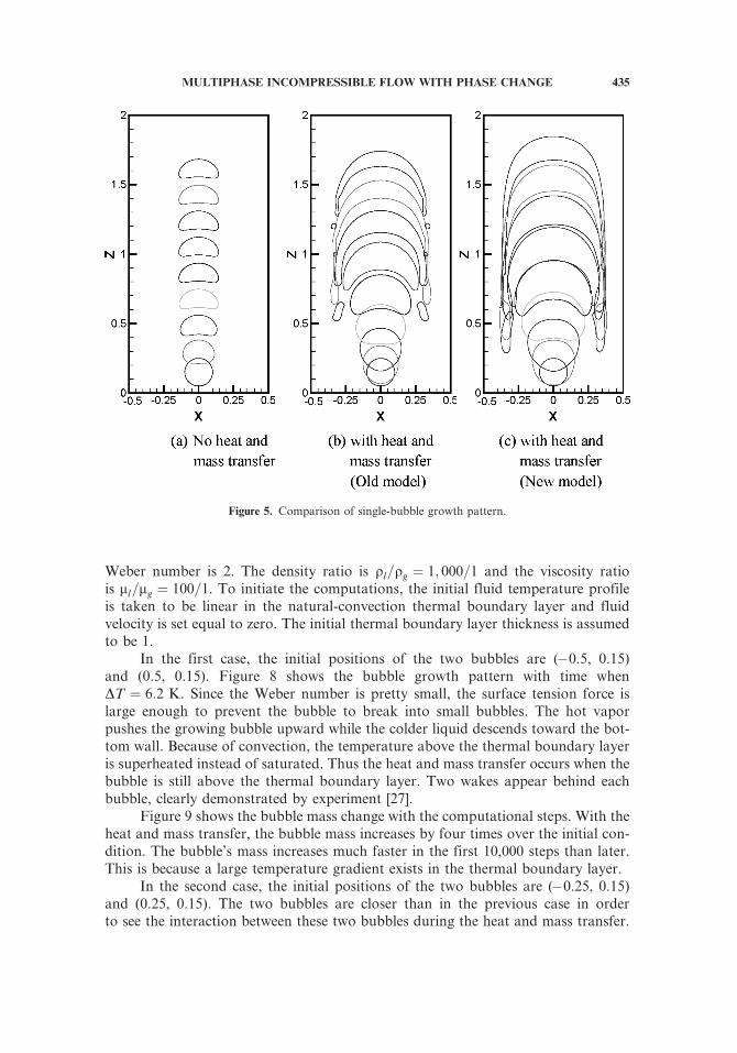
Figure 5a shows the bubble growth pattern with time when there is no heat andmass transfer. Figures 5b and 5c show the bubble growth pattern with time by usingthe old model and new model separately when DT ¼ 6:2 K. Compared with no heatand mass transfer, the bubble grows fast when under the thermal boundary layer.After that, the bubble grows slowly and begins to break into smaller bubbles.Because of the convection initialized by the bubble movement, the temperatureabove the thermal boundary layer is superheated instead of saturated. Thus the heatand mass transfer still occur when the bubble is above the thermal boundary layer,although they are much smaller than under the thermal boundary layer. By using themodified model, the mass transfer part has been simulated more accurately, so thatthe bubble grows faster than in the old model.

Figure 6 shows the bubble mass change with time by using two different models.By using the modified model, the bubble mass increases 463.6%, compared with248.5% in theoldmodel.This is because themodifiedmodel considers the interface con-dition more accurately and thus can simulate the mass transfer part more accurately.

Figure 7 shows the single-bubble growth pattern and temperature field duringthe nucleate boiling by using the old and modified models. Comparing them, wecan see the modified model captures more information at the interface so that themass increases faster and the bubble holds its shape better. This is because the subcell

Figure 3. Zero level set contour from time ¼ 0.2 to time ¼ 3.0.


conception has been used near the interface in the modified model and the masstransfer part can be simulated more accurately, which will affect the other terms,such as surface tension.

4.2. 2-D Multibubble Dynamic Interaction during Nucleate Boiling

The 2-D multibubbles computational domain is 2� 2 and the meshes are193� 193. The initial bubble radius is 0.1. The Reynolds number is 100 and the

Figure 4. History of water front location on solid surfaces in the dam break.


Weber number is 2. The density ratio is ql=qg ¼ 1; 000=1 and the viscosity ratiois ml=mg ¼ 100=1. To initiate the computations, the initial fluid temperature profileis taken to be linear in the natural-convection thermal boundary layer and fluidvelocity is set equal to zero. The initial thermal boundary layer thickness is assumedto be 1.

In the first case, the initial positions of the two bubbles are (�0.5, 0.15)and (0.5, 0.15). Figure 8 shows the bubble growth pattern with time whenDT ¼ 6:2 K. Since the Weber number is pretty small, the surface tension force islarge enough to prevent the bubble to break into small bubbles. The hot vaporpushes the growing bubble upward while the colder liquid descends toward the bot-tom wall. Because of convection, the temperature above the thermal boundary layeris superheated instead of saturated. Thus the heat and mass transfer occurs when thebubble is still above the thermal boundary layer. Two wakes appear behind eachbubble, clearly demonstrated by experiment [27].

Figure 9 shows the bubble mass change with the computational steps. With theheat and mass transfer, the bubble mass increases by four times over the initial con-dition. The bubble’s mass increases much faster in the first 10,000 steps than later.This is because a large temperature gradient exists in the thermal boundary layer.

In the second case, the initial positions of the two bubbles are (�0.25, 0.15)and (0.25, 0.15). The two bubbles are closer than in the previous case in orderto see the interaction between these two bubbles during the heat and mass transfer.

Figure 5. Comparison of single-bubble growth pattern.


Figure 10 shows the bubbles’ growth pattern with time when DT ¼ 6:2 K. Duringthe processing, the hot vapor pushes the growing bubble upward while the colderliquid descends toward the bottom wall. Because of the viscous fluid, bubble motionwill induce a vortex of the same sign in the computational domain. This vortex pairaccelerates the separation of the bubbles. The bubbles break into smaller bubbleswhen outside the thermal boundary. The lower parts of the broken bubbles in thethermal boundary layer grow faster because of the large temperature gradient.

Figure 11 shows the bubble mass change with the computational steps. Withthe heat and mass transfer, the bubble mass increases by three times over the initialcondition.

4.3. 3-D Single-Bubble Nucleate Boiling

The 3-D single-bubble computational domain is 1� 1� 2 and the meshes are41� 41� 81. The initial bubble radius is 0.1. The Reynolds number is 100 and theWeber number is 5. The density ratio is ql=qg ¼ 1; 000=1 and the viscosity ratio isml=mg ¼ 100=1. To initiate the computations, the initial fluid temperature profile istaken to be linear in the natural-convection thermal boundary layer and fluidvelocity is set equal to zero. The initial thermal boundary layer thickness is assumedto be 1 in this case.

Figure 6. Steps–mass comparison between two models.


Figure 12a shows the bubble growth pattern when DT ¼ 6:2 K. With the heatand mass transfer, the bubble grows fast. When the bubble is above the thermalboundary layer, it begins to deform from the top center. The deformation propa-gates along the radial direction and finally the bubble breaks up and forms a corollashape. This is significantly different from a no heat and mass transfer bubble rising,when the bubble shape holds because of a large surface tension force. If we take alook at the shape of the bubble from the bottom view, we find that the inside ofthe bubble became empty during the bubble expansion. When the surface tensioncannot maintain this ‘‘empty inside’’ bubble shape, the deformation begins.

Figure 12b shows the bubble mass change with time by using two differentmodels. By using the modified model, the bubble mass increases 1945.3% com-pared with 1089.5% in the old model. This is because the new model considersthe interface condition more accurately and can simulate the mass transfer partmore accurately.

Figure 7. Single-bubble growth pattern during nucleate boiling process.


Figure 8. Two separate bubbles’ growth pattern during nucleate boiling.


Figure 13 shows the bubble growth pattern and temperature field contoursduring the nucleate boiling process by using both the old and the modified models.After the bubble deformation, the mass begins to decrease a little because the roughmesh size cannot capture smaller bubbles. When the bubble is under the thermalboundary layer, the mass transfer part is big because of the large temperature gra-dient. When the bubble is above the thermal boundary layer, this part decreasesquickly.

5. CONCLUSION

In this article we have presented a numerical modeling for multiphase incom-pressible flow with phase change. The subcell conception has been introduced in thenew mass transfer model. The RKCN projection method has second-order temporalaccuracy for variable-density unsteady incompressible flows. The third-order ENOscheme and second-order semi-implicit Crank-Nicholson scheme is employed toupdate the convective and diffusion terms, respectively. The hyperbolic equationfor the level set function has been employed to implicitly capture the interface formultiphase flows. The four-level multigrid technique has been employed to enforcedivergence-free velocity incompressible flows. The numerical results show that thismethod can handle complex deformation of the interface and account for the effectof liquid–vapor phase change. The modified mass transfer model is more accurate

Figure 9. Bubble mass changes with computational steps.


Figure 10. Two separate bubbles’ growth pattern during nucleate boiling.


Figure 11. Bubble mass changes with computational steps.

Figure 12. 3-D bubble growth pattern when DT ¼ 6:2 K.


than the old model. The present numerical modeling has been further extended byemploying the ghost fluid method to calculate the heat and mass transfer at the inter-face. More results of multiphase incompressible flow with phase change by newmodeling will be given in the future.

REFERENCES

1. P. F. Peterson, R. Y. Bai, V. E. Schrock, and K. Hijikata, Droplet Condensation inRapidly Decaying Pressure Fields, J. Heat Transfer, vol. 114, pp. 194–200, 1992.

2. G. Son, V. K. Dhir, and N. Ramanujapu, Dynamics and Heat Transfer Associated with aSingle Bubble during Nucleate Boiling on a Horizontal Surface, J. Heat Transfer, vol. 121,pp. 623–631, 1999.

3. S. Welch and J. Wilson, A Volume of Fluid Based Method for Fluid Flows with PhaseChange, J. Comput. Phys., vol. 160, pp. 662–682, 2000.

4. D. Juric and G. Tryggvason, Computations of Boiling Flows, Int. J. Multiphase Flow,vol. 24, p. 387, 1998.

Figure 13. 3-D bubble growth pattern during nucleate boiling process.


5. D. Jamet, O. Lebaigue, N. Coutris, and J. M. Delhaye, The Second Gradient Theory forthe Direct Numerical Simulations of Liquid-Vapor Flows with Phase-Change, J. Comput.Phys., vol. 169, pp. 624–651, 2001.

6. F. H. Harlow and J. E. Welch, Numerical Calculation of Time-Dependent Viscous Incom-pressible Flow of Fluid with Free Surface, Phys. Fluids, vol. 8, no. 12, pp. 2182–2189,1965.

7. A. J. Chorin, Numerical Solution of Navier-Stokes Equations, J. Comput. Math., vol. 22,p. 745, 1968.

8. J. Kim and P. Moin, Application of Fractional-Step Method to Incompressible Navier-Stokes Equations, J. Comput. Phys., vol. 59, p. 108, 1985.

9. J. B. Bell, P. Colella, and H. M. Glaz, A Second-Order Projection Method for the Incom-pressible Navier-Stokes Equations, J. Comput. Phys., vol. 85, p. 257, 1989.

10. P. Gresho, On the Theory of Semi-implicit Projection Methods for Viscous Incompress-ible Flow and Its Implementation via a Finite Element Method That Also Introduces aNearly Consistent Mass Matrix, Part I: Theory, Int. J. Numer. Meth. Fluids, vol. 11,pp. 587–620, 1990.

11. H. Choi and P. Moin, Effects of the Computational Time Step on Numerical Solutions ofTurbulent Flow, J. Comput. Phys., vol. 101, p. 334, 1992.

12. S. V. Pantankar and D. B. Spalding, A Calculation Procedure for Heat, Mass andMomentum Transfer in Three-Dimensional Parabolic Flows, Int. J. Heat Mass Transfer,vol. 15, p. 1787, 1972.

13. S. V. Pantankar, Numerical Heat Transfer and Fluid Flow, McGraw-Hill, New York, 1980.14. D. B. Kothe and R. C. Mjolsness, IPPLE: A New Model for Incompessible Flows with

Free Surfaces, AIAA J., vol. 30, pp. 2694–2700, 1992.15. L. Chen, S. V. Garimella, J. A. Reizes, and E. Leonardi, The Development of a Bubble

Rising in a Viscous Liquid, J. Fluid Mech., vol. 387, pp. 61–96, 1999.16. M.-J. Ni and M. A. Abdou, Temporal Second-Order Accuracy of SIMPLE-Type

Methods for Incompressible Unsteady Flows, Numer. Heat Transfer B, vol. 46,pp. 529–548, 2004.

17. M.-J. Ni, S. Komori, and N. Morley, Projection Methods for the Calculation of Incom-pressible Unsteady Flows, Numer. Heat Transfer B, vol. 44, pp. 533–551, 2003.

18. M.-J. Ni, S. Komori, and M. Abdou, A Variable-Density Projection Method for Inter-facial Flows, Numerical Heat Transfer B, vol. 44, pp. 553–574, 2003.

19. J. K. Dukowicz and A. S. Dvinsky, Approximation Factorization as a High Order Split-ting for Implicit Incompressible Flow Equations, J. Comput. Phys., vol. 102, pp. 336–347,1992.

20. S. Osher and J. A. Sethian, Fronts Propagating with Curvature-Dependent Speed, Algo-rithms Based on Hamilton-Jacobi Formulation, J. Comput. Phys., vol. 79, pp. 12–49,1988.

21. A. Harten, B. Enquist, S. Osher, and S. Chakravarthy, Uniformly High Order EssentiallyNon-oscillatory Schemes, J. Comput. Phys., vol. 71, pp. 231–303, 1987.

22. R. P. Fedkiw, T. Aslam, B. Merriman, and S. Osher, A Non-oscillatory EulerianApproach to Interfaces in Multimaterial Flows (the Ghost Fluid Method), J. Comput.Phys., vol. 152, pp. 457–492, 1999.

23. J. U. Brackbill, D. B. Kothe, and C. Zemach, A ContinuumMethod for Modeling SurfaceTension, J. Comput. Phys., vol. 100, no. 2, pp. 335–354, 1992.

24. Y. C. Chang, T. Y. Hou, B. Merriman, and S. Osher, A Level Set Formulation of EulerianInterface Capturing Methods for Incompressible Fluid Flows, J. Comput. Phys., vol. 124,pp. 449–464, 1996.

25. M. Sussman, P. Smereka, and S. Osher, A Level Set Approach for Computing Solutionsto Incompressible Two-Phase Flow, J. Comput. Phys., vol. 20, pp. 1165–1191, 1994.


26. M. Sussman and E. Fatemi, An Efficient Interface-Preserving Level Set RedistancingAlgorithm and Its Application to Interfacial Incompressible Fluid Flow, J. Sci. Comput.,vol. 20, pp. 1156–1191, 1999.

27. R. Scardovelli and S. Zaleski, Direct Numerical Simulation of Free-Surface and Inter-facial Flow, Annu. Rev. Fluid Mech., vol. 31, p. 567, 1999.

28. D. Bhaga and M. E. Weber, Bubbles in Viscous Liquids: Shapes, Wakes and Velocities,J. Fluid Mech., vol. 105, pp. 61–85, 1981.

29. J. C. Martin and W. J. Moyce, An Experimental Study of the Collapse of Liquid Columnson a Rigid Horizontal Plane, Philosophical Transactions of the Royal Society of London.Series A, Mathe. Phys. Sci., vol. 244, pp. 312–324, 1952.


NUMERICAL MODELING FOR MULTIPHASE INCOMPRESSIBLE FLOW … publications/2005... · numerical...

Documents

Transcript of NUMERICAL MODELING FOR MULTIPHASE INCOMPRESSIBLE FLOW … publications/2005... · numerical...