Numerical methods for wave propagation in nonlinear acoustics
97
1/97 Examples 1D 2D/3D Future Conclusions Ref Numerical methods for wave propagation in nonlinear acoustics R´ egis Marchiano Universit ´ e Pierre et Marie Curie Institut Jean le Rond d’Alembert (UMR UPMC/CNRS 7190) [email protected] 22 Juin 2010 R´ egis Marchiano Ol´ eron 2010
Transcript of Numerical methods for wave propagation in nonlinear acoustics

1/97
Examples 1D 2D/3D Future Conclusions Ref
Numerical methods for wave propagation innonlinear acoustics
Regis Marchiano
Universite Pierre et Marie CurieInstitut Jean le Rond d’Alembert (UMR UPMC/CNRS 7190)
[email protected] Juin 2010
Regis Marchiano Oleron 2010

2/97
Examples 1D 2D/3D Future Conclusions Ref
Guidelines...
”[...] In general it is extremely valuable to understand where theequation one is attempting to solve comes from, since a goodunderstanding of the physics (or biology, etc ...) is generallyessential in understanding the development and behavior ofnumerical methods for solving the equation [...]”
R. J. LeVeque, Finite Difference Methods for Ordinaryand Partial Differential Equations[1]
Regis Marchiano Oleron 2010

3/97
Examples 1D 2D/3D Future Conclusions Ref
Propagation of nonlinear waves
Propagation in fluids
Dauxois, Oléron 2007
Propagation in solids
Barrière, Oléron 2007
Regis Marchiano Oleron 2010

4/97
Examples 1D 2D/3D Future Conclusions Ref
Propagation in complex media
Propagation in rocks
Johnson, Oléron 2007
Propagation in granular media
Regis Marchiano Oleron 2010

5/97
Examples 1D 2D/3D Future Conclusions Ref
NDE and medical acoustics
NDE
Van Abeele, Oléron 2007
Medical therapy and imaging
http://www.polyclinique-cotebasquesud.com/images/Lithotritie.jpg
Regis Marchiano Oleron 2010

6/97
Examples 1D 2D/3D Future Conclusions Ref
Shock waves propagation in air (BSN, sonic boom, ...)
Regis Marchiano Oleron 2010

7/97
Examples 1D 2D/3D Future Conclusions Ref
Flow instabilities
Aeroacoustics Musical acoustics
Regis Marchiano Oleron 2010

8/97
Examples 1D 2D/3D Future Conclusions Ref
Various examples of nonlinear acoustics
Which numerical methods ?
Dauxois, Oléron 2007
Regis Marchiano Oleron 2010

9/97
Examples 1D 2D/3D Future Conclusions Ref
Answer:
... It depends ...
Regis Marchiano Oleron 2010

10/97
Examples 1D 2D/3D Future Conclusions Ref
Table of content I
1 Various examples of nonlinear acoustics
2 Numerical Resolution of the Burgers equationNumerical resolution of Burgers equation - case withoutshocksNumerical resolution of Burgers equation - case withshocks
3 Higher dimensionsThe geometrical acousticsThe one-way methodsDirect computation
4 Future ...?
5 Conclusions
6 References
Regis Marchiano Oleron 2010
11/97
Examples 1D 2D/3D Future Conclusions Ref no shocks with shocks
The Burgers equation
For plane waves or in 1D in fluids, the simplest equation is theBurgers equation:
∂p
∂x=
β
2ρ0c30
∂p2
∂τ+
δ
2c30
∂2p
∂τ2,
with β the nonlinear term and δ the absorption one. Ifabsorption is neglected, it yields the inviscid Burgers equation:
∂p
∂x=
β
2ρ0c30
∂p2
∂τ,
How to solve that equation numerically? ....There exist severalways.
Regis Marchiano Oleron 2010

12/97
Examples 1D 2D/3D Future Conclusions Ref no shocks with shocks
Numerical resolution of Burgers equation - casewithout shocks
1 The inviscid Burgers equationFinite Difference MethodPoisson SolutionFrequency Domain Solution
2 The Burgers equationFrequency domainTime DomainHopf-Cole transformation
Regis Marchiano Oleron 2010

13/97
Examples 1D 2D/3D Future Conclusions Ref no shocks with shocks
Numerical resolution of the inviscid Burgers equation -case without shocks - Finite Difference Method
∂u
∂t+∂f(u)∂x
= 0 (1)
with f(u) = u2/2 for fluids or f(u) = u3/3 for solids.
Regis Marchiano Oleron 2010

14/97
Examples 1D 2D/3D Future Conclusions Ref no shocks with shocks
Numerical resolution of the inviscid Burgers equation -case without shocks - Finite Difference Method
Basic Idea [2, 3, 1]: g(x, t)→ gni = g(xi, tn),∂g
∂t≈gn+1i − gni
∆t+O(∆t) or
∂g
∂t≈gn+1i − gn−1
i
2∆t+O(∆t2).
Various schemes exist:Explicit (Natural, Lax-Wendroff, Lax-Friederichs,
Leap-Frog,...)gn+1i − gni
∆t= L(fn)
Implicitgn+1i − gni
∆t= L(fn+1)
Crank-Nicolsongn+1i − gni
∆t=
12(L(gn+1) + L(gn)
)Regis Marchiano Oleron 2010

15/97
Examples 1D 2D/3D Future Conclusions Ref no shocks with shocks
Numerical resolution of the inviscid Burgers equation -case without shocks - Finite Difference Method
Natural scheme for the Burgers equation:
un+1i − uni
∆t= −
Funi+1 − Funi−1
2∆x,
with Funi = f(uni ) and un1 = u(xn)Unstable ![3]Lax-Friederichs scheme:
un+1i =
uni+1 + uni2
− ∆t2∆x
(Funi+1 − Funi−1
),
with Funi = f(uni ) and un1 = u(xn)Conditionally stable [3]: ∆t/∆x < 1/|u|
Regis Marchiano Oleron 2010
16/97
Examples 1D 2D/3D Future Conclusions Ref no shocks with shocks
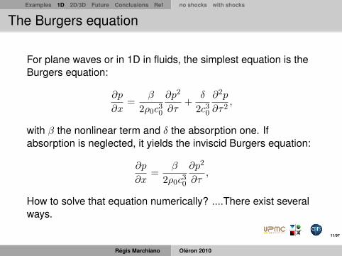
Numerical resolution of the inviscid Burgers equation-case without shocks - Finite Difference Method
Nx = Nt = 5000f(u) = u2/2 f(u) = u3/3
Regis Marchiano Oleron 2010

17/97
Examples 1D 2D/3D Future Conclusions Ref no shocks with shocks
Numerical resolution of the inviscid Burgers equation-case without shocks - Finite Difference Method
Same as previously but ∆x and ∆t are divided by 5(Nx = Nt = 5000).
f(u) = u2/2 f(u) = u3/3
Finite Difference methods for inviscid Burgers equationpresent... strong dissipation!Regis Marchiano Oleron 2010

18/97
Examples 1D 2D/3D Future Conclusions Ref no shocks with shocks
Numerical resolution of the inviscid Burgers equation-case without shocks - Poisson Solution
There exists an implicit solution for the inviscid Burgersequation:
u(x, t) = u0(ξ)
x = ξ − t.u0(ξ)
That solution can be used up to the shock formation distance:∂x
∂ξ6= 0.
Regis Marchiano Oleron 2010

19/97
Examples 1D 2D/3D Future Conclusions Ref no shocks with shocks
Numerical resolution of the inviscid Burgers equation -case without shocks - Poisson Solution
f(u) = u2/2 f(u) = u3/3
Regis Marchiano Oleron 2010
20/97
Examples 1D 2D/3D Future Conclusions Ref no shocks with shocks
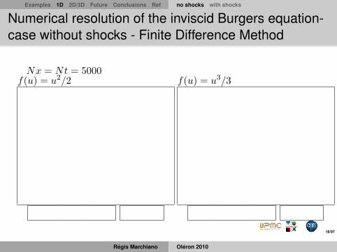
Numerical resolution of the inviscid Burgers equation -case without shocks - Spectral method
The basic idea is closed to the Fubini solution. Solution ofinviscid Burgers equation:
∂p
∂x=
12∂p2
∂t,
is sought as:
p(x, t) =+∞∑
m=−∞Am(x) exp(−imt).
So, the problem to solve is now a coupled ODE set:
dAmdx
= − i2m
+∞∑m=−∞
Am−r(x)Ar(x)
For details see [4, 5, 6]Regis Marchiano Oleron 2010

21/97
Examples 1D 2D/3D Future Conclusions Ref no shocks with shocks
Numerical resolution of the inviscid Burgers equation -case without shocks - Spectral method
For the resolution, the system is truncated :
dAm∂x
= − i2m
+M∑m=−M
Am−r(x)Ar(x),
once the Am are computed, the pressure is reconstructed:
p(x, t) =+∞∑
m=−∞Am(x) exp(−imt).
Regis Marchiano Oleron 2010

22/97
Examples 1D 2D/3D Future Conclusions Ref no shocks with shocks
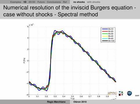
Numerical resolution of the inviscid Burgers equation -case without shocks - Spectral method
M = 10, 20, 30, 40, 50 and 100.
0 0.1 0.2 0.3 0.4 0.5 0.6 0.7 0.8 0.9 1x 10⁻⁶
−6
−4
−2
0
2
4
6x 10⁵
T [s]
P [P
a]
0 0.1 0.2 0.3 0.4 0.5 0.6 0.7 0.8 0.9 1x 10⁻⁶
−6
−4
−2
0
2
4
6x 10⁵
T [s]
P [P
a]
0 0.1 0.2 0.3 0.4 0.5 0.6 0.7 0.8 0.9 1x 10⁻⁶
−6
−4
−2
0
2
4
6x 10⁵
T [s]
P [P
a]
0 0.1 0.2 0.3 0.4 0.5 0.6 0.7 0.8 0.9 1x 10⁻⁶
−6
−4
−2
0
2
4
6x 10⁵
T [s]
P [P
a]
0 0.1 0.2 0.3 0.4 0.5 0.6 0.7 0.8 0.9 1x 10⁻⁶
−6
−4
−2
0
2
4
6x 10⁵
T [s]
P [P
a]
0 0.1 0.2 0.3 0.4 0.5 0.6 0.7 0.8 0.9 1x 10⁻⁶
−6
−4
−2
0
2
4
6x 10⁵
T [s]
P [P
a]
Regis Marchiano Oleron 2010
23/97
Examples 1D 2D/3D Future Conclusions Ref no shocks with shocks
Numerical resolution of the inviscid Burgers equation -case without shocks - Spectral method
0 0.1 0.2 0.3 0.4 0.5 0.6 0.7 0.8 0.9 1x 10⁻⁶
−6
−4
−2
0
2
4
6x 10⁵
T [s]
P [P
a]
M=10M=20M=30M=40M=50M=100
Figure:
Regis Marchiano Oleron 2010

24/97
Examples 1D 2D/3D Future Conclusions Ref no shocks with shocks
Numerical resolution of the inviscid Burgers equation -case without shocks - Spectral method
0 10 20 30 40 50 60 70 80 90 100−10
−9
−8
−7
−6
−5
−4
m
log(
Pw)
M=100M=50M=40M=30M=20M=10
Regis Marchiano Oleron 2010

25/97
Examples 1D 2D/3D Future Conclusions Ref no shocks with shocks
Conclusion
+ −Finite Difference Method simplicity absorption
Poisson Solution nonlinearities continuous wavestransient waves
Spectral method freq. interactions oscillationscontinuous waves transient waves
Regis Marchiano Oleron 2010

26/97
Examples 1D 2D/3D Future Conclusions Ref no shocks with shocks
Numerical resolution of the Burgers equation - casewithout shocks
The Burgers equation is:
∂p
∂x=
β
2ρ0c30
∂p2
∂τ2+
δ
2c30
∂2p
∂τ2,
Frequency Domain SolutionTime Domain SolutionHopf-Cole transformation
Regis Marchiano Oleron 2010

27/97
Examples 1D 2D/3D Future Conclusions Ref no shocks with shocks
Numerical resolution of the Burgers equation - casewithout shocks - Frequency domain approximation
As for the inviscid Burgers equation, the solution is sought as:
p(x, t) =+∞∑
m=−∞Am(x) exp(−imt).
There is an additional term in the set of ODE:
dAmdx
= αAm(x)m2 − i
2m
+M∑m=−M
Am−r(x)Ar(x),
The numerical procedure is the same as previously.
Regis Marchiano Oleron 2010

28/97
Examples 1D 2D/3D Future Conclusions Ref no shocks with shocks
Numerical resolution of the Burgers equation - casewithout shocks - Time domain approximation
Basic idea: resolution in time by using the power of Poissonsolution without drawbacks of numerical absorptionSolution: technique of the operator splitting:
1∂p
∂x=
β
2ρ0c30
∂p2
∂τ2, (implicit Poisson Solution)
2∂p
∂x=
δ
2c30
∂2p
∂τ2. (finite difference method)
!! !
1- Nonlinearitiesimplicit Poisson Solution
2 - Absorptionfinite difference method
Regis Marchiano Oleron 2010

29/97
Examples 1D 2D/3D Future Conclusions Ref no shocks with shocks
Numerical resolution of the Burgers equation - casewithout shocks - Hopf-Cole approximation
The Burgers equation:
∂u
∂t= u
∂u
∂x+ α
∂2u
∂x2,
The Hopf-Cole transformation:
u(x, t) = −2αθxθ
One obtains the heat equation (linear PDE!):
∂θ
∂t= α
∂2θ
∂x2
It is possible to solve it numerically thanks to classical methods.
Regis Marchiano Oleron 2010

30/97
Examples 1D 2D/3D Future Conclusions Ref no shocks with shocks
Conclusion
+ −Frequency domain absorption oscillations
nonlinearitiescontinuous waves
Time domain nonlinearities absorptiontransient waves
Pseudo-spectral nonlinearities FFT, IFFTabsorption
Hopf-cole transformation 1D nD
Regis Marchiano Oleron 2010

31/97
Examples 1D 2D/3D Future Conclusions Ref no shocks with shocks
Numerical resolution of the inviscid Burgers equation -case with shocks - Poisson Solution
f(u) = u2/2 f(u) = u3/3
Regis Marchiano Oleron 2010
32/97
Examples 1D 2D/3D Future Conclusions Ref no shocks with shocks
Numerical resolution of Burgers equation - case withshocks
The theory (cf 1st lecture by F. Coulouvrat) shows that twoingredients are needed beyond the shock formation distance:
The ’mathematical’ solution of the Burgers equation(whatever the method) ;The weak shock theory ;
From the 1st part, the first point is addressed. For the secondpoints, there are two strategies:
Shock capturing (introduction of numerical dissipation);Shock fitting (explicit treatment of the shock);
Regis Marchiano Oleron 2010

33/97
Examples 1D 2D/3D Future Conclusions Ref no shocks with shocks
Numerical resolution of Burgers equation - case withshocks - shock capturing
Basic idea: to introduce numerical viscosity in theneighborhood of shocksAn example: McDonald and Ambrosiano scheme (1984):
1 standard scheme for the regular part2 correction of the flux near the shocks
For more details, see Leveque (1992).
Regis Marchiano Oleron 2010
34/97
Examples 1D 2D/3D Future Conclusions Ref no shocks with shocks
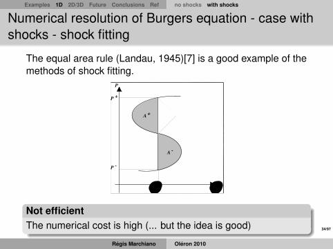
Numerical resolution of Burgers equation - case withshocks - shock fitting
The equal area rule (Landau, 1945)[7] is a good example of themethods of shock fitting.
Formulation géométrique : la loides aires égales
Landau (1944)
Loi des aires égales : le choc est placé de telle façon que les airesdes 2 lobes de part et d’autre du choc sont égales
!
A+ = A"
P
!!C
P -
P +
A -
A +
Not efficientThe numerical cost is high (... but the idea is good)
Regis Marchiano Oleron 2010

35/97
Examples 1D 2D/3D Future Conclusions Ref no shocks with shocks
Numerical resolution of Burgers equation - case withshocks - shock fitting
The Burgers-Hayes method [8, 9, 10]: Poisson solution for thepotential + max of the potential
!3 !2 !1 0 1 2 30
0.05
0.1
0.15
0.2
0.25
0.3
0.35
!3 !2 !1 0 1 2 3!0.4
!0.3
!0.2
!0.1
0
0.1
0.2
0.3
0.4
!3 !2 !1 0 1 2 3!0.4
!0.3
!0.2
!0.1
0
0.1
0.2
0.3
0.4
Φ(X,T )Φ(X + ∆X,T )Φphys(X + ∆X,T )
Regis Marchiano Oleron 2010

36/97
Examples 1D 2D/3D Future Conclusions Ref no shocks with shocks
Numerical resolution of Burgers equation - case withshocks - shock fitting
The Burgers-Hayes method needs:1 Compute the potential ;2 Compute the Poisson solution ;3 Compute the max of the Poisson solution (for quadratic
nonlinearities) ;4 Compute the original variable ;
Efficient and elegantfor time domain simulation
Regis Marchiano Oleron 2010

37/97
Examples 1D 2D/3D Future Conclusions Ref Rays One-way Direct
The original sin
Now, 1D is a piece of cake, what about 2D/3D ?
Figure: Michel-Ange, Chapelle Sixtine, 1512
The troubles begin !
Regis Marchiano Oleron 2010

38/97
Examples 1D 2D/3D Future Conclusions Ref Rays One-way Direct
A first example
Simulation of sonic boom:
domain 18km×35km×60km.f0 ≈ 3.4Hz; c0 ≈ 340m.s−1 soλ0 ≈ 100msimulation with 100 harmonics impliesλ100 ≈ 1mgood discretization implies ≈ 6 pts/λmeshes are:18.103∗6×35.103∗6×60.103∗6 ≈ 8.1015
time integration dt ≈ 1, 5.10−3s,∆T ≈1min, NT ≈ 40.103
The direct simulationis prohibitive (not necessarily impossible) and alternative wayshave to be found.
Regis Marchiano Oleron 2010

39/97
Examples 1D 2D/3D Future Conclusions Ref Rays One-way Direct
Several ways to follow
Geometrical acoustics ;One way methods ;Nonlinear Wave Equation ;The FDTD.
Regis Marchiano Oleron 2010

40/97
Examples 1D 2D/3D Future Conclusions Ref Rays One-way Direct
Nonlinear geometrical acoustics
High frequency;plane wave assumption;λ << L;λ << LH .
Regis Marchiano Oleron 2010
41/97
Examples 1D 2D/3D Future Conclusions Ref Rays One-way Direct
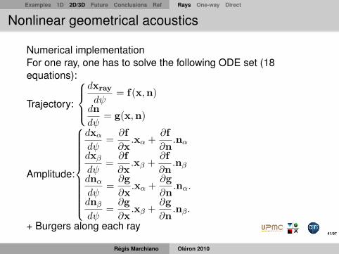
Nonlinear geometrical acoustics
Numerical implementationFor one ray, one has to solve the following ODE set (18equations):
Trajectory:
dxray
dψ= f(x,n)
dndψ
= g(x,n)
Amplitude:
dxαdψ
=∂f∂x
.xα +∂f∂n
.nαdxβdψ
=∂f∂x
.xβ +∂f∂n
.nβdnαdψ
=∂g∂x
.xα +∂g∂n
.nα.
dnβdψ
=∂g∂x
.xβ +∂g∂n
.nβ.
+ Burgers along each ray
Regis Marchiano Oleron 2010

42/97
Examples 1D 2D/3D Future Conclusions Ref Rays One-way Direct
Nonlinear geometrical acoustics
+ −easy caustics
efficient (fast) shadow zoneinterferences
diffraction
For more details, see Olaf Gainville’s lecture on Friday.
Regis Marchiano Oleron 2010

43/97
Examples 1D 2D/3D Future Conclusions Ref Rays One-way Direct
One-way approximations
Regis Marchiano Oleron 2010

44/97
Examples 1D 2D/3D Future Conclusions Ref Rays One-way Direct
Basic idea of the one-way approximations
Basic idea: factorization of the wave equation.Similar to the derivation of the 1D Burgers equation (see 1stlecture):
∂2p
∂x2− 1c20
∂2p
∂t2= 0, (2)
That equation can be factorized easily:
(∂p
∂x− 1c0
∂p
∂t
) (∂p
∂x+
1c0
∂p
∂t
)= 0 (3)
Propagation towards −x Propagation towards+x
Regis Marchiano Oleron 2010

45/97
Examples 1D 2D/3D Future Conclusions Ref Rays One-way Direct
One way approximation in 1D
The ”one-way” equation is:
∂p
∂x+
1c
∂p
∂t= 0, (4)
Considering that the sound velocity depends on the
instantaneous pressure: c ≈ c0 +βp
ρ0c0, it yields the Burgers
equation:
∂P
∂X=
12∂P 2
∂T(5)
with P = p/P0, X = x/LC , LC = 1/(kβM), M acoustical Machnumber, β ≈ 3.5 (in water), k the wavenumber andT = ω0(t− x/c0)
Regis Marchiano Oleron 2010

46/97
Examples 1D 2D/3D Future Conclusions Ref Rays One-way Direct
One-way approximation in 2D/3D
Let us start from the Lighthill-Westerwelt equation:
∂2pa∂t2
− c20∆pa =β
ρ0c20
∂2p2a
∂t2
That equation can be expressed in delayed time τ = t− x/c0:
2c0∂2pa∂τ∂x
− c20(∂2pa∂x2
+ ∆⊥pa
)=
β
ρ0c20
∂2p2a
∂t2
How to factorize that equation ? formal factorization is possiblebut introduces non integer operators !
Regis Marchiano Oleron 2010

47/97
Examples 1D 2D/3D Future Conclusions Ref Rays One-way Direct
One-way approximation in 2D/3D
Several strategies exist to factorize the wave equation:1 Parabolic approach (KZ, wide angle, NPE, ...)2 Other approches
Regis Marchiano Oleron 2010

48/97
Examples 1D 2D/3D Future Conclusions Ref Rays One-way Direct
One-way approximation in 2D/3D: the parabolicapproximation
Derivation of the KZ equation
2c0∂2pa∂x∂τ
− c20(∂2pa∂x2
+ ∆⊥pa
)=
β
ρ0c20
∂2p2a
∂t2
Parabolic approximation:1c0
∂pa∂τ
>>∂pa∂x
2c0∂2pa∂x∂τ
− c20
∂2pa∂x2
+∂2pa∂y2
=β
ρ0c20
∂2p2a
∂t2.
Khokhlov-Zabolotskaya equation [11] (or NPE [12]) :
2c0∂2pa∂x∂τ
− c20∂2pa∂y2
=β
ρ0c20
∂2p2a
∂τ2.
Regis Marchiano Oleron 2010

49/97
Examples 1D 2D/3D Future Conclusions Ref Rays One-way Direct
One-way approximation in 2D/3D: the wide anglenonlinear equation
Derivation of the wide-angle nonlinear equation:
2c0∂2pa∂x∂τ
− c20(∂2pa∂x2
+ ∆⊥pa
)=
β
ρ0c20
∂2p2a
∂t2
The linear parabolic approximation:∂2pa∂x∂τ
− c02∂2pa∂y2
= 0 so,∂3pa∂x2∂τ
− c02∂3pa∂x∂y2
= 0
It yields the wide-angle nonlinear wave equation [13, 14]:
2c0∂3pa∂x∂τ2
− c20[(
∂
∂τ+c02∂
∂x
)∂2pa∂y2
]=
β
ρ0c20
∂3p2a
∂τ3
Regis Marchiano Oleron 2010

50/97
Examples 1D 2D/3D Future Conclusions Ref Rays One-way Direct
One-way approximation in 2D/3D: go further ?
−2 −1.5 −1 −0.5 0 0.5 1 1.5−1.5
−1
−0.5
0
0.5
1
1.5
KZ
KX
The process can be used again and again to improve theapproximation.
ButThe order of the equation increases (so additional BC arerequired)The improvement is not so important (see results of thenumerical simulations)Regis Marchiano Oleron 2010

51/97
Examples 1D 2D/3D Future Conclusions Ref Rays One-way Direct
How to solve the KZ equation ?
The KZ equation [11, 15] is:
∂P
∂X∂τ=∂2P
∂Y 2+ µ
∂2P 2
∂τ2,
with µ the nonlinear parameter, α the absorption parameter.3 families of numerical solvers exist:
1 Spectral resolution ;2 Time domain resolution.3 Pseudo-spectral resolution ;
Regis Marchiano Oleron 2010
52/97
Examples 1D 2D/3D Future Conclusions Ref Rays One-way Direct
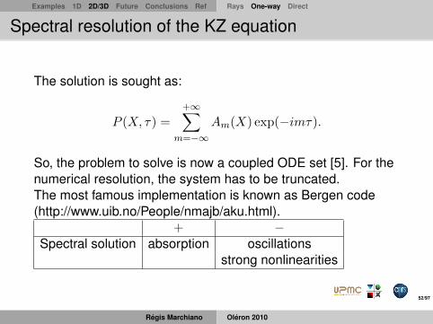
Spectral resolution of the KZ equation
The solution is sought as:
P (X, τ) =+∞∑
m=−∞Am(X) exp(−imτ).
So, the problem to solve is now a coupled ODE set [5]. For thenumerical resolution, the system has to be truncated.The most famous implementation is known as Bergen code(http://www.uib.no/People/nmajb/aku.html).
+ −Spectral solution absorption oscillations
strong nonlinearities
Regis Marchiano Oleron 2010

53/97
Examples 1D 2D/3D Future Conclusions Ref Rays One-way Direct
Pseudo-Spectral and temporal resolutions the KZequation
The pseudo-spectral and the temporal methods of resolution ofthe KZ equation rely on the split-step procedure [16, 17].
∂2P
∂X∂τ=
∂2P
∂Y 2+ µ
∂2P 2
∂τ2
!! !
Diffraction
FFT + FD + IFFTTemporal solver
Nonlinearities
Temporal solverTemporal solver
Regis Marchiano Oleron 2010

54/97
Examples 1D 2D/3D Future Conclusions Ref Rays One-way Direct
Time domain resolution the KZ equation
This family of solvers has been introduced by Lee and Hamiltonet al. [18].
∂2P
∂X∂τ=
∂2P
∂Y 2+ µ
∂2P 2
∂τ2
∂P
∂X=∫ τ
−∞
∂2P
∂Y 2dτ ′
Implicit scheme: P ki = L(P ki )+Trapezoidal rule
∂2P
∂X∂τ= µ
∂2P 2
∂τ2
Integration:∂P
∂X= µ
∂P 2
∂τThis is the Burgers equation. Itcan be solved by methodspresented in section I.
Regis Marchiano Oleron 2010

55/97
Examples 1D 2D/3D Future Conclusions Ref Rays One-way Direct
Time domain resolution the KZ equation: Exemple
N wave focusing on a cusp caustic [19]
ConvergentWavefront
P
T
N wave
Regis Marchiano Oleron 2010

56/97
Examples 1D 2D/3D Future Conclusions Ref Rays One-way Direct
Pseudo-Spectral resolution the KZ equation
This family of solvers has been introduced by Bakhvalov et al.[20].
∂2P
∂X∂τ=
∂2P
∂Y 2+ µ
∂2P 2
∂τ2
∂2P
∂X∂τ=∂2P
∂Y 2
FFT: iω∂P
∂X=∂2P
∂Y 2
Implicit scheme: P ki = L(P ki )Resolution of a linear system.IFFT: P (Z = ∆Z, τ)
∂2P
∂X∂τ= µ
∂2P 2
∂τ2
Integration:∂P
∂X= µ
∂P 2
∂τThis is the Burgers equation. Itcan be solved by methodspresented in section I.
Regis Marchiano Oleron 2010

57/97
Examples 1D 2D/3D Future Conclusions Ref Rays One-way Direct
Pseudo-Spectral resolution the KZ equation: Example
The reflexion of shock waves on a rigid surface
z
y
θ
θ<15°
Incident wave
Reflected wave
Periodic sawtooth wave
Regis Marchiano Oleron 2010

58/97
Examples 1D 2D/3D Future Conclusions Ref Rays One-way Direct
Pseudo-Spectral resolution the KZ equation: Example
The reflexion of shock waves on a rigid surfaceθ = 5o θ = 3o θ = 1o
a = 1.81 a = 0.91 a = 0.36
a) KZ code, b) Experiment and c) linear KZ equation
Regis Marchiano Oleron 2010

59/97
Examples 1D 2D/3D Future Conclusions Ref Rays One-way Direct
Pseudo-Spectral resolution the KZ equation: Example
Piston: (a) analytical solution, (b) KZ simulation
x/ !
y/ !
(a)0 5 10 15
−10
0
10−40
−20
0
x/ !
y/ !
(b)0 5 10 15
−10
0
10−40
−20
0
x/ !
y/ !
(c)0 5 10 15
−10
0
10−40
−20
0
x/ !y/
!
(d)0 5 10 15
−10
0
10−40
−20
0
Regis Marchiano Oleron 2010

60/97
Examples 1D 2D/3D Future Conclusions Ref Rays One-way Direct
Numerical resolution of the wide-angle nonlinearequation
The procedure is the same as for the KZ equation: split-stepprocedure + resolution of the simpler equations
x/ !
y/ !
(a)0 5 10 15
−10
0
10−40
−20
0
x/ !
y/ !
(b)0 5 10 15
−10
0
10−40
−20
0
x/ !
y/ !
(c)0 5 10 15
−10
0
10−40
−20
0
x/ !
y/ !
(d)0 5 10 15
−10
0
10−40
−20
0
x/ !
y/ !
(a)0 5 10 15
−10
0
10−40
−20
0
x/ !y/
!
(b)0 5 10 15
−10
0
10−40
−20
0
x/ !
y/ !
(c)0 5 10 15
−10
0
10−40
−20
0
x/ !
y/ !
(d)0 5 10 15
−10
0
10−40
−20
0
(a) analytical(c) KZ(d) WA
Regis Marchiano Oleron 2010

61/97
Examples 1D 2D/3D Future Conclusions Ref Rays One-way Direct
Summary
+ −Frequency domain absorption oscillations
nonlinearitiescontinuous waves
Time domain nonlinearities absorptiontransient waves
Pseudo-spectral nonlinearities FFT, IFFTabsorption
continuous wavesadditional effects
Regis Marchiano Oleron 2010

62/97
Examples 1D 2D/3D Future Conclusions Ref Rays One-way Direct
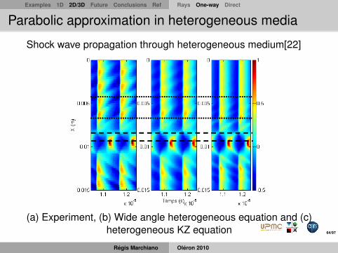
Parabolic approximation in heterogeneous media
The parabolic equations (KZ or wide-angle) can be extended totake into account propagation in weakly heterogeneous media[21, 22]Sound speed fluctuations: c(x, y) = c0 + c0(x, y)Generalized KZ equation:
∂2pa∂x∂τ
− c02∂2pa∂y2
=β
ρ0c02
∂2p2a
∂τ2+c20(x, y)
2c03
∂2pa∂τ2
.
!! !
Diffraction Heterogenities Nonlinearities
Regis Marchiano Oleron 2010

63/97
Examples 1D 2D/3D Future Conclusions Ref Rays One-way Direct
Shock wave propagation through heterogeneous medium
c0 ch c0
Regis Marchiano Oleron 2010
64/97
Examples 1D 2D/3D Future Conclusions Ref Rays One-way Direct
Parabolic approximation in heterogeneous media
Shock wave propagation through heterogeneous medium[22]!"#$%&'()&"*+,+-.(*#+(*-%/+0+/)+1$)$."-$*$&)$'+23%)&4%/'+ +++++++++++++++++++
!"#$
!
5&-3./+678+9/4.$'/*)()&"*+'4()&":)/24"./%%/+#3+;1(24+#/+4./''&"*+2/'3.$+<=+-(3;1/>+
/)+'&23%$+(?/;+%@$A3()&"*+,+-.(*#+(*-%/+0+<(3+2&%&/3>+/)+(?/;+%@$A3()&"*+4(.(B&(%/+<=+
#."&)/>+#(*'+%/+4%(*+C";(%+<DE622>+#@3*/+1$)$."-$*$&)$+#/+#&(2F)./+G+22+<-(3;1/>8+H/'+
*&?/(3B+#/+4./''&"*+'"*)+./4.$'/*)$'+/*+;"3%/3.+/)+*".2(%&'$+4(.+%(+4./''&"*+C";(%/+
2(B&2(%/8+
!
%&'! ()*+,'! -&! ,.&''/01! '/+234'! '2.! 35*6&! -&! ,.0,*7*8/01! *9&(! 3&'! 4:2*8/01'!
;!7.*1-! *173&!<! =>/7?! $@A! &1! 8/.&8B! &8! ,*.*6/*3&! =>/7?! $@A! &1! ,0/18/334B! '018! &1! 8.C'! D01!
*((0.-! &1! *+,3/82-&! &8! &1! ,)*'&! *9&(! 3&! .4'238*8! &6,4./+&18*3?! E&23&! 3*! ,)*'&!
-5&6,*1'/01! &'8! 21! ,&2! +0/1'! D/&1! -4(./8&! &6,4./+&18*3&+&18?! F1! .&8.029&! /(/A! 3&'!
.4'238*8'!-4GH!,.4'&184'!*2!()*,/8.&!"!-*1'!3&!(*'!;!'8*1-*.-!<?!%5*,,.06/+*8/01!;!7.*1-!
*173&!<!&'8!:2*'/+&18!/1-/'(&.1*D3&!-&!35*,,.06/+*8/01!'8*1-*.-?!!
I!"!++!-&!35*6&!-&!,.0,*7*8/01!=>/7?!$#BA!3&!()*+,!-&!,.&''/01!'2.!21&!,4./0-&!
8&+,0.&33&! &'8! +0-/J/4! ,*.! 3501-&! (K3/1-./:2&! -/JJ.*(84&! ,*.! 35)484.07414/84! '2.! 3*!
,4./0-&!()0/'/&A!+*/'!*2''/! '2.! 3*!,4./0-&!,.4(4-&18&! =(J?!>/7?!$LB?!%&'!-&26! 3/71&'!&1!
(a) Experiment, (b) Wide angle heterogeneous equation and (c)heterogeneous KZ equation
Regis Marchiano Oleron 2010

65/97
Examples 1D 2D/3D Future Conclusions Ref Rays One-way Direct
Numerical Resolution of the KZ equation in 3D
∂2Φ∂X∂τ
= ∆⊥P + µ∂
∂τ
(∂Φ∂τ
)2
+Hc∂2Φ∂τ2
!! !
Diffraction effects
∂2Φ∂X∂τ
= ∆⊥Φ
→ spectral method
Nonlinear effects
∂2Φ∂X∂τ
= µ∂
∂τ
(∂Φ∂τ
)2
→ Burgers-Hayesmethod
Heterogeneouseffects
∂2Φ∂X∂τ
= Hc∂2Φ∂τ2
→ analytical method
Regis Marchiano Oleron 2010

66/97
Examples 1D 2D/3D Future Conclusions Ref Rays One-way Direct
Numerical Resolution of the KZ equation in 3D
source: P (X = 0, Y, Z, T ) = P0 sin(2πf0T ) exp(−(Y 2 + Z2)σ2
))
Temporal evolution
RMS pressure Phase
Regis Marchiano Oleron 2010

67/97
Examples 1D 2D/3D Future Conclusions Ref Rays One-way Direct
Numerical Resolution of the KZ equation in 3D
RMS pressureRegis Marchiano Oleron 2010

68/97
Examples 1D 2D/3D Future Conclusions Ref Rays One-way Direct
Numerical Resolution of the KZ equation in 3D
Sound speed profil: c(x, y, z) = c0 + 100y
!0.1
0
0.1
0.1
0.2
0.3
0.4
0.5
!0.1
!0.05
0
0.05
0.1
XZ
Y
1490
1492
1494
1496
1498
1500
1502
1504
1506
1508
1510
!0.10
0.10.05 0.1 0.15 0.2 0.25 0.3 0.35 0.4 0.45 0.5 0.55
!0.1
!0.05
0
0.05
0.1
X
Z
Y
0.1
0.2
0.3
0.4
0.5
0.6
0.7
0.8
0.9
white curve = acoustical ray
Regis Marchiano Oleron 2010

69/97
Examples 1D 2D/3D Future Conclusions Ref Rays One-way Direct
Summary on the parabolic approaches
Advantagesefficient ;versatile ;very popular ;
Drawbacksangular limitation ;no backscattering ;
Regis Marchiano Oleron 2010

70/97
Examples 1D 2D/3D Future Conclusions Ref Rays One-way Direct
Beyond the parabolic
Is it possible to keep the advantages of parabolic approach,while avoiding the drawbacks ?Existing answers:
1 Christopher and Parker phenomenological approach [23] ;2 Wojcik et al.,’s TAWE method [24];3 HOWARD method.
These methods are still one-way methods
Regis Marchiano Oleron 2010

71/97
Examples 1D 2D/3D Future Conclusions Ref Rays One-way Direct
Christopher and Parker phenomenological approach[23]
problem, in order to gain advantages in computational effi- ciency, to develop a formalism that does not require the parabolic approximation, and to allow for multiple layer propagations. Basically, our methodology utilizes an incre- mental propagation of an axially symmetric field from some plane at axial distance z from the source to a parallel plane at distance z + Az. The concept is illustrated in Fig. 1. The normal velocity radial profiles ui (z,r) of a fundamental (solid line) and higher harmonics u, (z,r) (dashed lines), n = 2 to N, are propagated together in Az steps. Note in Fig. 1 that to highlight the nonlinear effect over Az, the initial field consists of the fundamental harmonic only.
First, the diffraction effect is accounted for by utilizing the (Fourier) convolution theorem and a discrete Hankel trans- form (DHT). The recently developed DHT •8 offers great computational savings 19 as compared to the two-dimension- al discrete fast Fourier transform. Computing diffraction in- volves multiplying the DHT of each harmonic radial profile by its appropriate linear transfer function H, (z,R) [the DHT of the point spread function h• (z,r) ], which is equiva- lent to convolution in the original spatial domain, as implied by Huygen's principle. An inverse DHT gives the desired diffracted harmonic radial profile u'• (z + Az, r) (the prime notation indicates intermediate results) for each harmonic present in the propagation. This diffraction operator is de- picted in Fig. 2. Note also the presense of attenuation in the form of an attenuated transfer function. The nonlinear effect is accounted for by advancing the diffracted and discretely sampled field forward on a point-by-point basis over an
equivalent incremental Az distance without diffraction, but with accretion and depletion of harmonics according to a temporal frequency domain solution to Burgers' equation (FDSBE).20-22 That is, for some radial position ri, the nor- mal velocities u', (z + Az, ri) are modified by nonlinear mechanisms to u, (z + Az, r• ) as if the acoustic velocity rep- resented a plane wave traveling in the direction of the phase front at ri. This concept is illustrated in Fig. 3.
The model also accounts for the effects of refraction and reflection (but not multiple reflections) in the case of propa- gation through multiple, parallel layers of fluid medium. •9 The model's use of a novel harmonic-limiting scheme for the FDSBE 23 makes possible some previously intractable high- intensity (shocked) propagations. The model's approach appears to be a departure from other nonlinear models in its extensive use of transform (spatial and temporal) tech- niques. There are well-known computational advantages in- herent in transform operations, but also pitfalls in imple- mentations as discussed extensively in our companion paper on linear propagation. 19 These pitfalls can be avoided by appropriately windowing the point spread function h or its transform H.
Conceptually, our approach is somewhat akin to the work of Pestorius and Blackstock, 24'25 who treated the nondif- fraeting propagation of plane waves in two domains using incremental advances. In the time domain, waveform distor-
DIFFRACTION & ATTENUATION SUBSTEP
INCREMENTAL PROPAGATION I Partk•e Velocity
U • U • HANKEL TRANSFORM J r R
MULTIPLY BY ATTENUATED
INVERSE DIFFRACTION NONUNEAR HANKEL TRANSFORM 8tJBSl'EP 8UBSTEP
FIG. 1. Illustration depicting the concept of incremental field propagation using substeps for the diffraction and nonlinear operators. Shown are radial (transaxial) plots of normal velocity magnitude of the fundamental (solid lines) and the higher harmonics (dotted lines) at different stages in the propagation substeps. To highlight the nonlinear effect over Az, the figure depicts an initial single harmonic field.
FIG. 2. The diffraction substep with its discrete Hankel transform useage (here applied to one harmonic using the RFSC approach).
489 J. Acoust. Soc. Am., Vol. 90, No. 1, July 1991 P.T. Christopher and K. d. Parker: Nonlinear diffractive field 489
Christopher and Parker, JASA, 1991
1 Resolution of thewave equation
2 Resolution of theBurgers equation
Regis Marchiano Oleron 2010

72/97
Examples 1D 2D/3D Future Conclusions Ref Rays One-way Direct
Woicjik et al.’s TAWE method [24]
TAWE = Time Averaged Wave Envelopes method
the given point in space as the superposition of sinusoidalwaves unbounded in time. The vertical lines in Fig. 2(A)
correspond to the coefficients Cl of the decomposition.They are calculated after the substitution of Eq. (5) into
d0
),( zPm x
QmP
),( zzPm ∆+x
x
x
y
dmin (x, z) P(x, z)
z
nonlinear step
diffraction & absorption step
S
dmax(x, z)
z∆
Fig. 1. Explanation of the incremental wave propagation using incremental steps for the diffraction, absorption and non-linear distortion operators. Hered0 denotes the diameter of the source; dmax and dmin are the maximum and minimum distances of the field point (x,z) from the source. The pressure at (x,z)is propagated to the field point (x,z + Dz) in two steps.
n
V(x, z, n) = F [ P(x, z, τ) ]
V1
V2Vm
0 2πτ
P(x, z,τ)
Cn(x, z)
… + … +
A
B
C
n max
dn
mnim ezP
−),τ,(x
niezP 2
2 ), τ,(−
xni
ezP 1), τ,(1−
x
Nn~
11= Nn~
22=Nmnm~=
Fig. 2. Decomposition of the disturbance, P(x,z,s). (C) shows the representation of P(x,z,s) as Re[R(x,z,s)]. (B) shows the decomposition of P(x,z,s) intothe sum of M wavelet-like sinusoidal pulses, Pmðx; z; sÞ expð#im~NsÞ. (A) shows the Fourier spectrum, V(x,z,n). The N spectral components, Cn(x,z)(shown as the solid lines – in (A)) are calculated in the CM. The Fourier spectra V mðx; z; n# m~NÞ of the individual wavelets (shown as thin solid lines – in(A)), are calculated in the TAWE method and sum into the total spectrum identical to V(x,z,n).
314 J. Wojcik et al. / Ultrasonics 44 (2006) 310–329
[Wojcik et al., Ultrasonics, 2006]
Regis Marchiano Oleron 2010

73/97
Examples 1D 2D/3D Future Conclusions Ref Rays One-way Direct
HOWARD
HOWARD = Heterogeneous One-Way Approximation forResolution of Diffraction
2c0∂2pa∂x∂τ
−c20(∂2pa∂x2
+∂2pa∂y2
)− β
ρ0(x)c20(x)∂2p2
a
∂τ2
−(
1− c20c20(x)
)∂2pa∂τ2
+c20(x)ρ0(x)
([∂pa∂x− 1c0
∂pa∂τ
]∂ρ0
∂x+∂pa∂y
∂ρ0
∂y
)=0
No approximation on the diffraction term ;High frequency approximation on the nonlinear term ;Wide angle approximation on the heterogeneous term(Heterogeneous terms are assumed to be weak).
Regis Marchiano Oleron 2010

74/97
Examples 1D 2D/3D Future Conclusions Ref Rays One-way Direct
HOWARD
Numerical resolution: the splitting operator technique
2c0∂2pa∂x∂τ
−c20(∂2pa∂x2
+∂2pa∂y2
)− β
ρ0(x)c20(x)∂2p2
a
∂τ2
−(
1− c20c20(x)
)∂2pa∂τ2
+c20(x)ρ0(x)
([∂pa∂x− 1c0
∂pa∂τ
]∂ρ0
∂x+∂pa∂y
∂ρ0
∂y
)=0
!! !
Diffraction
Spectral method
Heterogeneities
Finite difference
Nonlinearities
Burgers-Hayes
Regis Marchiano Oleron 2010

75/97
Examples 1D 2D/3D Future Conclusions Ref Rays One-way Direct
Step 1: diffraction
Diffraction: Spectral resolution
2c0∂2Φ∂x∂τ
−c20(∂2pa∂x2
+∂2pa∂y2
)= 0
Angular spectrum method [?, 23, 25]:ˆpa(X, kY , ω) = FY {FT {Φ(X,Y, T )}}
D∂2 ˆpa∂X2
+ iω∂ ˆpa∂X−K2
Yˆpa = 0.
2nd order ODE => 2 solutions (propagation towards +x et −x).
ˆpa(X+∆X,KY , ω) =
ˆpa(X,KY , ω) exp
−iω +√
4DK2Y − ω2
2D
∆X if 4DK2Y ≥ ω2
ˆpa(X,KY , ω) exp
−iω + i√ω2 − 4DK2
Y
2D
∆X if 4DK2Y < ω2.
[1] Goodman et al., 1976 ; [2] Christopher et al., 1991, [3] Marchiano et al., 2008
Regis Marchiano Oleron 2010

76/97
Examples 1D 2D/3D Future Conclusions Ref Rays One-way Direct
Dispersion
−2 −1.5 −1 −0.5 0 0.5 1 1.5−1.5
−1
−0.5
0
0.5
1
1.5
KZ
KX
Regis Marchiano Oleron 2010

77/97
Examples 1D 2D/3D Future Conclusions Ref Rays One-way Direct
Step 2 : heterogeneities
heterogeneities: Finite differences method (pseudo-spectral method)
2c0∂2Φ∂x∂τ
−(
1− c20c20(x)
)∂2Φ∂τ2
+c20(x)ρ0(x)
([∂Φ∂x− 1c0
∂Φ∂τ
]∂ρ0
∂x+∂Φ∂y
∂ρ0
∂y
)=0
Resolution in Fourier space with an implicit scheme (possibilityto add absorption).
Regis Marchiano Oleron 2010

78/97
Examples 1D 2D/3D Future Conclusions Ref Rays One-way Direct
HOWARD
x/
y/
(a: analytique)
0 5 10 15
15
10
5
0
5
10
15 40
30
20
10
0
x/
y/
(b : HOWARD)
0 5 10 15
15
10
5
0
5
10
15 40
30
20
10
0
x/
y/
(c : KZ)
0 5 10 15
15
10
5
0
5
10
15 40
30
20
10
0
x/
y/
(d : Grand angle)
0 5 10 15
15
10
5
0
5
10
15 40
30
20
10
0
Regis Marchiano Oleron 2010

79/97
Examples 1D 2D/3D Future Conclusions Ref Rays One-way Direct
Propagation of sonic boom in turbulent atmosphere
Regis Marchiano Oleron 2010

80/97
Examples 1D 2D/3D Future Conclusions Ref Rays One-way Direct
Propagation of sonic boom in turbulent atmosphere
Regis Marchiano Oleron 2010

81/97
Examples 1D 2D/3D Future Conclusions Ref Rays One-way Direct
Conclusions
Today, one-way methods are the standard for manyapplications. But remember that there is a severe drawback(due to their advantages!): they are one-way.
They are not adapted for nonlinear propagation in complexmedia.
Regis Marchiano Oleron 2010

82/97
Examples 1D 2D/3D Future Conclusions Ref Rays One-way Direct
Direct computation
Very intensive but ...Various approaches exist:Sparrow and Raspet, JASA, 1991 [?]
FDTD: Finite Difference Time DomainResolution of a system of 1st order equations (nonlinear +dissipative effects)2D simulation of the propagation of spark pulse inhomogeneous media(NX ×NY )=322×322, NT = 4000.Computer: Cray 2.
Regis Marchiano Oleron 2010

83/97
Examples 1D 2D/3D Future Conclusions Ref Rays One-way Direct
Direct computation
Sparrow and Raspet, JASA, 1991(a) {c)
• ..... :=-:'•.. •,•;•.,--•. "'".":::'•-:.¾!:.':...! '.: .-::' ::' :-.'.-:'• : ": -' : .... ' :' ' ':: :.'.':'%'•½A•. ' :'.-*:•,;-'! :.:.::-:;:-,:.-::.:7.:::.-:-: ================================= '- :--'•':.::-- ";:-i"i:"-i:::':::" :-':::Y ::: i- !: •:-..'- :i-...':..:'.-i:?:'-..:::+: i-:..:-'
.i:::-:: ß ' '.': :':':':i:i:.:•; ' ::.i..%%t.--. ........ ' ........... '.: ,:-: .:::
.... . ..... . :•.-..:•.•.. .;..-:.:-:-:-:-.-:-: :.:.:.:.:-:.:.: :...::.'.!::.::
:.:!::..::... :.. " '"'::.'...•.: ..i '- ' '. .... -' ":':'.':..!..ii,:•.•: • ::.:'%"v ' ß 'i : ß ' ß: ': ':"': ":" :' "i'."::'":".:: :"';'""::•'"::•':'"""" ' -•:•' ':'& •i :'"" •:i':::':' :' ' ' '
lb) (d)
ß .. -•.."?•.• .- :,'.•-:,: •.',,-.,':i..i' :.-.'.i: ,.ii :ii E: i::. •:i :':i:.:::.:r':' :', ': "::':':"':'*'½.:,, i:• ::"• '"' •:'" ' ::::::::::::::::::::::::::::::::::::: •':" :'"':"'"':•:'":'"'""•':
'::.4. ,:•, • ; ' .:" :i.• .-'- ' -,-':' .il, :.:.i :L .' :': ': .ii':: "i:: , i .:: ,: :i: i ::: ':::' ' ' : .... :'• • """: :'::"::' :::':::':':'::":: ': ':':'"'":: ,'--•::, "::.i'"::."!: J!;:•! :::.•:":.::::.i:i:L•:.?• i:: !::'::::::.:i::.
FIG. 4. Mach stem development for one of the simulation runs. Each snapshot is 4 cm long in d and extends from I 0175 to 3'0 cm high in Zl (a) The initial condition at time zero. (b)-(d) Snapshots at times 40, 80, and ! 20Fs in a coordinate system moving forward at speed 343 m/s. Positive acoustic pressures are the darker shades, while the negative acoustic pressures are light.
2.4 ÷
2.2
2
1.8
1.6
1.4
1.2
amplificatiønb• factor
a
d
incident angle in degrees
2'0 4'0 6'0 8'0
FIG. 5. Oblique reflection amplification factor versus angle in degrees for fixed free-field incident peak pressures. When the angle is 0 deg, the wave front is locally normally incident on the hard surface, and when the angle is 90 deg, the wave front is locally grazing. (a) Free-field incident peak pres- sureis 15.0 kPa, 177.5 dB, (b) I0.0 kPa, 174 dB, (c) 5.0 kPa, 168 dB, and (d) 2.5 kPa, 162 dB.
add the effects of molecular relaxation dissipation. In the future the numerical technique will model the propagation of acoustic waves from explosions over natural ground sur- faces and the results will be compared to published experi- mental data.
ACKNOWLEDGMENTS
This research was supported by the United States Army Construction Engineering Research Laboratory (USA- CERL), Champaign, IL. The National Center for Super- computing Applications (NCSA), Champaign, IL provided the supercomputing resources.
• D. H. Trivett and A. L Van Buren, "Propagation of plane, cylindrical, and spherical finite amplitude waves," J. Acoust. Soc. Am. 69, 943-949 (1981).
2S. I. Aanonsen, T. Barkve, J. Naze Tj6tta and S. TjCtta, "Distortion and
2690 J. Acoust. Soc. Am., Vol. 90, No. 5, November 1991 V. W, Sparrow and R. Raspet: Finite amplitude wave propagation 2690
Downloaded 18 Jun 2010 to 134.157.34.104. Redistribution subject to ASA license or copyright; see http://asadl.org/journals/doc/ASALIB-home/info/terms.jsp
Regis Marchiano Oleron 2010

84/97
Examples 1D 2D/3D Future Conclusions Ref Rays One-way Direct
Direct computation
Pinton et al., IEEE Trans. Ultrason. Ferroelectr. Freq. Control,2010 [26]
FDTD: Finite Difference Time DomainResolution of the Westervelt equation (2nd orderderivatives, nonlinear + dissipative effects)3D simulation of nonlinear propagation of ultrasonic wavesgenerated by a transducer(LX × LY × LZ)=1.5cm×1.5cm×1.5cm, f0 = 2MHz,λ = 0.075cm.(NX ×NY ×NZ)=833×833×833, NT = 10000.Cluster: 56 proc, 128GB, Linux, MPI
For more details, see Gianmarco’s talk on thursday.
Regis Marchiano Oleron 2010

85/97
Examples 1D 2D/3D Future Conclusions Ref Rays One-way Direct
Direct computation
cm
cm
10 5 0 5 10
0
5
10
1535
30
25
20
15
10
5
0
Regis Marchiano Oleron 2010

86/97
Examples 1D 2D/3D Future Conclusions Ref
New trends ?
Various new trends exist. Let us focus on the parallelization.Again, various paradigms exist:
1 SPMD = Single Program Multiple Data (OpenMPIstandard)
2 SIMD = Single Instruction Multiple Data (OpenMPstandard)
3 CPU vs. GPU
Regis Marchiano Oleron 2010

87/97
Examples 1D 2D/3D Future Conclusions Ref
OpenMP vs MPI
Shared memory
P1 P2 P3 P4
SIMD (OpenMP)
P1 P2 P3 P4
SPMD (MPI)
M1 M2 M3 M4
Message PassingInterface
Regis Marchiano Oleron 2010

88/97
Examples 1D 2D/3D Future Conclusions Ref
MPI example: Domain Decomposition
Regis Marchiano Oleron 2010

89/97
Examples 1D 2D/3D Future Conclusions Ref
GPU vs CPU
CPU = Central Processing UnitIn June 2010: a standard configuration has ≈ 10 cores.Numerous clusters exist through the world from ≈ 100 cores inthe labs to ≈ 100.000 cores for the best ones (TOP 500 : 1st
Oak Ridge National Laboratory 224162 cores ! )GPU = Graphics Processing UnitIn June 2010: on 1 GPU = (≈ 500 cores, 6Go memory, doubleprecision). Possibility to have a cluster of GPU.
New technologies...... need new methodologies to take advantage of the availablepower. Think out of the box !
Regis Marchiano Oleron 2010
90/97
Examples 1D 2D/3D Future Conclusions Ref
Conclusions
Lot of methods exist ;No-one is the best one ;Everything begins with a good modeling ;Follow the physics to find the appropriate method ;Numerical methods are fun (numerical experiments) ;Think out of the box !
Regis Marchiano Oleron 2010

91/97
Examples 1D 2D/3D Future Conclusions Ref
References I
R. J. Leveque, Finite Difference Methods for Ordinary andPartial Differential Equations (SIAM) (2007).
G. Cohen, Higher-order numerical methods for transientwave equations (Springer-Verlag) (2002).
D. Euvrard, Resolution numerique des equations auxderivees partielles (Masson) (1994).
A. Korpel, “Frequency approach to non-linear dispersivewaves”, J. Acoust. Soc. Am. 67, 1954–1958 (1980).
S. I. Aanonsen, T. Barkve, J. N. Tjotta, and S. Tjotta,“Distortion and harmonic generation in the nearfield of afinite amplitude sound beam”, J. Acoust. Soc. Am. 75,749–768 (1984).
Regis Marchiano Oleron 2010

92/97
Examples 1D 2D/3D Future Conclusions Ref
References II
R. Fernando, “Modelisation et simulation du buzz sawnoise”, Ph.D. thesis, Universite Pierre et Marie Curie(2010).
L. Landau, “On shock waves at large distances from theplace of their origin”, J. Phys. USSR 9, 496–500 (1945).
J. M. Burgers, “A mathematical model illustrating the theoryof turbulence”, Adv. Appl. Mech. 1, 171–199 (1948).
W. D. Hayes, R. C. Haefeli, and H. E. Kulsrud, “Sonic boompropagation in a stratified atmosphere with computerprogram”, Technical Report CR-1299, NASA (1969).
F. Coulouvrat, “A quasi-analytical shock solution for generalnonlinear progressive waves”, Wave Motion online (2008).
Regis Marchiano Oleron 2010

93/97
Examples 1D 2D/3D Future Conclusions Ref
References III
E. A. Zabolotskaya and R. V. Khokhlov, “Quasi-plane wavesin the nonlinear acoustics of confined beams”, Sov. Phys.Acoust. 15, 35–40 (1969).
B. E. McDonald and W. A. Kuperman, “Time domainformulation for pulse propagation including nonlinearbehavior at a caustic”, J. Acoust. Soc. Am. 81, 1406–1417(1987).
J. F. Claerbout, Fundamentals of geophysical dataprocessing: with applications to petroleum pospecting(McGraw-Hill (New-York)) (1976).
L. Ganjehi, “Ondes de choc acoustiques en milieuheterogene, des ultrasons au bang sonique”, Ph.D. thesis,Univeriste Pierre et Marie Curie (2008).
Regis Marchiano Oleron 2010

94/97
Examples 1D 2D/3D Future Conclusions Ref
References IV
V. P. Kuznetsov, “Equation of nonlinear acoustics”, Sov.Phys. Acoust. 16, 467–470 (1970).
W. F. Ames, Numerical methods for partial differentialequations (Academic Press (San Diego)) (1977).
R. J. Leveque, Numerical Methods for Conservation Laws(Birkhauser) (1992).
Y. S. Lee and M. F. Hamilton, “Time-domain modeling ofpulsed finite-amplitude sound beams”, J. Acoust. Soc. Am.97 (1995).
R. Marchiano, F. Coulouvrat, and J. L. Thomas, “Nonlinearfocusing of acoustic shock waves at a caustic cusp”, J.Acoust. Soc. Am. 117, 566 – 577 (2005).
Regis Marchiano Oleron 2010

95/97
Examples 1D 2D/3D Future Conclusions Ref
References V
N. S. B. et al., Nonlinear Theory of Sound Beams(American Institute of Physics) (1987).
P. Blanc-Benon, P. Lipkens, L. Dallois, M. F. Hamilton, andD. T. Blackstock, “Propagation of finite amplitude soundthrough turbulence: Modeling with geometrical acousticsand the parabolic approximation”, J. Acoust. Soc. Am.487–498 (2002).
L. Ganjehi, R. Marchiano, F. Coulouvrat, and J. L. Thomas,“Evidence of the wave front folding of sonic boom by alaboratory scale deterministic experiment of shock waves ina heterogeneous medium”, J. Acoust. Soc. Am. 124, 57–71(2008).
Regis Marchiano Oleron 2010

96/97
Examples 1D 2D/3D Future Conclusions Ref
References VI
T. Christopher and K. Parker, “New approaches tononlinear diffractive field propagation”, J. Acoust. Soc. Am.90, 488–499 (1991).
J. Wojcik, A. Nowicki, P. A. Lewin, P. E. Bloomfield,T. Kujawska, and L. Filipczynski, “Wave envelopes methodfor description of nonlinear acoustic wave propagation”,Ultrasonics 44, 310–329 (2006).
R. Marchiano, F. Coulouvrat, L. Ganjehi, and J. L. Thomas,“Numerical investigation of the properties of nonlinearacoustical vortices through weakly heterogeneous media”,Physical Review E 77, 016605 (2008).
Regis Marchiano Oleron 2010

97/97
Examples 1D 2D/3D Future Conclusions Ref
References VII
G. Pinton, J. Dahl, S. Rosenzweig, and G. E. Trahey, “Aheterogeneous nonlinear attenuating full- wave model ofultrasound”, IEEE Trans. Ultrason. Ferroelectr. Freq.Control 56, 474–488 (2010).
Regis Marchiano Oleron 2010