R. HiptmairL. ScarabosioC. Urzua Torres

Spring Term 2015

Numerical Methods for PartialDifferential Equations

ETH ZurichD-MATH

Homework Problem Sheet 3

Problem 3.1 Fourier Spectral Galerkin Scheme for Two-Point BoundaryValue Problem

In [NPDE, Section 1.5.2.1] you learned about the discretization of 2-point boundary value prob-lems based on global polynomials using integrated Legendre polynomials as basis. The imple-mentation for a linear BVP was presented in [NPDE, § 1.5.48].

This problem is focused on another variant of spectral Galerkin discretization, which relies onnon-polynomial trial and test spaces and, again, employs globally supported basis functions. Thistime the solution will be approximated by linear combinations of trigonometric functions. Youwill be asked to implement the Galerkin discretization in MATLAB and to study its convergencein a numerical experiment, cf [NCSE, Thm. 9.1.4].

We consider the linear variational problem: seek u ∈ C10,pw([0, 1]) such that∫ 1

0

σ(x)du

dx(x)

dv

dx(x) dx =

∫ 1

0

f(x)v(x) dx, ∀v ∈ C10,pw([0, 1]), (3.1.1)

cf. [NPDE, Eq. (1.4.23)]. For the discretization of (3.1.1) we may use a so-called Fourier-spectralGalerkin method, which boils down to a Galerkin method using the trial and test space

VN,0 := span{sin(πx), sin(2πx), . . . , sin(Nπx)} , (3.1.2)

and the basis function already given in the definition (3.1.2). It is related the spectral Galerkinscheme discussed in [NPDE, Section 1.5.2.1].

(3.1a) Show that the functions specified in (3.1.2) really provides a basis of VN,0.

HINT: First establish orthogonality of the basis functions with respect to the inner product

(f, g)L2(0,1) :=

∫ 1

0

f(x)g(x) dx .

Then recall that a basis of a finite dimensional vector space is a maximal linearly independentsubset.

Solution: We only have to show that the sines are linearly independent. In fact, they are orthog-onal. For i = j:∫ 1

0

sin(iπx) sin(jπx) dx =1

2

∫ 1

0

[cos((i− j)πx)− cos((i+ j)πx)] dx = 0,

as both i+ j and i− j are nonzero.

Problem Sheet 3 Page 1 Problem 3.1

(3.1b) Which basis should be used for the Fourier spectral scheme, if we had to approximatefunctions in the space C1

0,pw([a, b]) for fixed a < b, instead of the space C10,pw([0, 1]).

HINT: Read [NPDE, § 1.5.41].

Solution: The transformed basis in this case would be

VN,0([a, b]) = span{sin(π(x− a)/h), sin(2π(x− a)/h), . . . , sin(Nπ(x− a)/h)},

with h = b− a.

(3.1c) Since (3.1.1) is a linear variational problem, any Galerkin discretization will lead toa linear system of equations. For the case σ ≡ 1 compute its matrix for the Galerkin schemerelying on VN,0 and the trigonometric basis specified in (3.1.2). Discuss structural properties ofthe matrix like sparsity, symmetry, regularity.

Solution: We need to compute the matrix entries

Ai,j = ijπ2

∫ 1

0

cos(iπx) cos(jπx) dx.

Using the identity

cos(iπx) cos(jπx) =1

2[cos((i− j)πx) + cos((i+ j)πx)],

we see as in (3.1a) that the off-diagonal terms are all zero. Then

Ai,i =i2π2

2

∫ 1

0

(1 + cos(2iπx)) dx =i2π2

2.

So

A =π2

2

1

49

. . .N2

.

This matrix is diagonal, thus both sparse and symmetric.

(3.1d) Write a MATLAB function

function A = getGalMat(sigma,N)

that computes the Galerkin matrix for the Fourier spectral Galerkin scheme for (3.1.1). Heresigma is a handle to the coefficient function σ. The evaluation of the integrals should be doneby means of a 3N -point Gaussian quadrature formula on [0, 1].

HINT: The nodes and weights of the Gaussian quadrature rules on [a, b] can be computed by theMATLAB function [x,w] = gauleg(a,b,n,tol), which is available for download.

Solution: See Listing 3.1.

Problem Sheet 3 Page 2 Problem 3.1

Listing 3.1: Computation of the Galerkin matrix1 f u n c t i o n C = getGalMat(sigma, N)2

3 [x,w] = gauleg(0,1,3*N);4

5 C = cos(pi*x*(1:N));6 % C(k,i) = cos(pi i x_k)

7

8 D = bsxfun(@times, C, sigma(x));9 D = bsxfun(@times, D, w);

10 % D(k,i) = cos(pi i x_k) sigma(x_k) w_k

11

12 C = C’ * D;13 % C(i,j) = sum_k cos(pi i x_k) cos(pi j x_k) sigma(x_k)

w_k

14

15 C = bsxfun(@times, C, 1:N);16 C = bsxfun(@times, C, (1:N)’);17 C = piˆ2 * C;18

19 end

(3.1e) Write a function

function phi = getrhsvector(f,N)

that computes the right-hand side vector for the Fourier spectral Galerkin discretization with Nbasis functions. The routine should rely on 3N -point Gaussian quadrature for the evaluation ofthe integrals.

Solution: See Listing 3.2.

Listing 3.2: Computation of the right-hand side vector1 f u n c t i o n phi = getrhsvector(f, N)2

3 [x,w] = gauleg(0,1,3*N);4

5 C = s i n(pi*x*(1:N));6 C = bsxfun(@times, C, f(x));7 phi = C’ * w;8

9 end

(3.1f) For σ(x) = 1cosh(sin(πx))

, f(x) = π2 sin(πx), determine an approximate solution of(3.1.1) by means of the Fourier spectral scheme introduced above. Create a suitable plot ofthe L2-norm and L∞-norm of the discretization error versus the number N of unknowns forN = 2, 3, . . . , 14 and, thus, investigate the convergence of the method [NCSE, Remark 9.1.4].

Problem Sheet 3 Page 3 Problem 3.1

Figure 3.1: Exact and approximate solution for N = 3.

The computation of the norms should be done approximately by means of numerical quadrature(equidistant trapeziodal rule with 105 points) and sampling (in 105 equidistant points), respec-tively, see [NPDE, Rem. 1.6.19].

HINT: The exact solution of the 2-point boundary value problem is

u(x) = sinh(sin(πx)).

Solution:

See Figure 3.1 for the approximate and exact solution at N = 3, Figure 3.2 for the convergenceplots and Listing 3.3 for the code used.

To compute the L2([a, b])-error (here [a, b] = [0, 1]) we use a composite trapeziodal rule withN + 1 equidistant points x0, . . . , xN∫ a

b

f(x) dx ≈ b− a

N

(f(x0)

2+

N−1∑i=1

f(xi) +f(xN)

2

)=

b− a

N

N∑i=1

f(xi),

where in the last step we used the periodicity of f , i.e., f(x0) = f(a) = f(b) = f(xN).

To estimate the rate of the exponential convergence, we do the following consideration for theerror e

e ≈ e−γnδ ⇐⇒ log e ≈ −γnδ ⇐⇒ log log e ≈ log(−γ) + log(nδ) = δ log n+ log−γ

Then we do a polyfit of the last term and obtain the best matching polynomial in x = log n andobtain δx+ x0, and we recompute γ as γ = −ex0 . We implement this in Listing 3.3 and obtain asimilar convergence for both normsL-inf convergence exponential with gamma: 1.4904 and delta: 1.2291

Problem Sheet 3 Page 4 Problem 3.1

Figure 3.2: Convergence for subproblem (3.1f).

L-2 convergence exponential with gamma: 1.7698 and delta: 1.1627.Note that the parameter 0 < δ < ∞ (high values are good) is more important than γ (which isoften omitted). The plots looks like a staircase, this comes from the fact, that this particular exactsolution uses only every second function in the space VN,0.

Listing 3.3: Convergence estimates for (3.1f)1 nvals = 2:14;2 M = 10ˆ5;3 sigma = @(x) ones( s i z e(x))./cosh( s i n(pi*x));4 f = @(x) piˆ2* s i n(pi*x);5 exact = @(x) s inh( s i n(pi*x));6

7 xpts = l i n s p a c e(0,1,M+1)’;8 xpts = xpts(2:end-1);9

10 l2err = [];11 lierr = [];12

13 f o r N = nvals14 A = getGalMat(sigma, N);15 L = getrhsvector(f, N);16 mu = A \ L;17

18 approx = evaltrigsum(mu, M);19 err = abs(approx - exact(xpts));20

Problem Sheet 3 Page 5 Problem 3.1

21 l2err = [l2err; s q r t(sum(err.ˆ2)/M)];22 lierr = [lierr; max(err)];23 end24

25 semi logy(nvals, lierr, ’bo-’);26 hold on; gr id on;27 p l o t(nvals, l2err, ’ro-’);28 xl im([1, 15]);29 x l a b e l(’N’);30 y l a b e l(’Error’);31 l egend(’Lˆ\infty’, ’Lˆ2’);32

33 P = p o l y f i t( l o g(nvals), l o g( l o g(lierr’)),1);34 gamma_inf=- r e a l(exp(P(2)));35 delta_inf=P(1);36

37 di sp([’L-inf convergence exponential with gamma: ’num2str(gamma_inf) ’ and delta: ’ num2str(delta_inf) ]);

38 Q = p o l y f i t( l o g(nvals), l o g( l o g(l2err’)), 1);39 gamma_2=- r e a l(exp(Q(2)));40 delta_2=Q(1);41 di sp([’L-2 convergence exponential with gamma: ’

num2str(gamma_2) ’ and delta: ’ num2str(delta_2) ]);42

43 p l o t(nvals, exp(-gamma_inf.*nvals.ˆdelta_inf));44 hold off;

(3.1g) Carry out the investigations requested in subproblem (3.1f) for

σ(x) =

{2 for |x− 1

2| < 1

4,

1 elsewhere,f ≡ 1 ,

this time using N = 2, 4, 8, 16, 32, 64, 128, 256, 512, 1024. What kind of convergence do youobserve? Relate with the observation made in subproblem (3.1f) and try to explain.

HINT: The exact solution is

u(x) =

{364

+ 14x− 1

4x2 |x− 1

2| < 1

4,

12x− 1

2x2 elsewhere.

Also recall the observations made in [NPDE, Exp. 1.6.31].

Solution:

See Figure 3.3 for the convergence plots and Listing 3.4 for the code used. The convergence isalgebraic with rates 1 for the L∞-norm and 1.25 for the L2-norm.

Listing 3.4: Convergence estimates for subproblem (3.1f)1 nvals = 2.ˆ(1:10);

Problem Sheet 3 Page 6 Problem 3.1

Figure 3.3: Convergence for subproblem (3.1f).

2 M = 10ˆ5;3 inside = @(x) abs(x-0.5) < 0.25;4 outside = @(x) 1 - inside(x);5 sigma = @(x) (1+inside(x)).*ones( s i z e(x));6 f = @(x) ones( s i z e(x));7 temp = @(x) 0.25*x - 0.25*x.ˆ2;8 exact = @(x) (1+outside(x)).*temp(x) +

inside(x).*ones( s i z e(x))*3/64;9

10 xpts = l i n s p a c e(0,1,M+1)’;11 xpts = xpts(2:end-1);12

13 l2err = [];14 lierr = [];15

16 f o r N = nvals17 A = getGalMat(sigma, N);18 L = getrhsvector(f, N);19 mu = A \ L;20

21 approx = [evaltrigsum(mu, M)];22 err = abs(approx - exact(xpts));23

24 l2err = [l2err; s q r t(sum(err.ˆ2)/M)];25 lierr = [lierr; max(err)];26 end

Problem Sheet 3 Page 7 Problem 3.1

27

28 l o g l o g(nvals, lierr, ’bo-’);29 hold on; gr id on;30 p l o t(nvals, l2err, ’ro-’);31 xl im([1, 2000]);32 x l a b e l(’N’);33 y l a b e l(’Error’);34 l egend(’Lˆ\infty’, ’Lˆ2’);35

36 P = p o l y f i t( l o g(nvals), l o g(lierr’), 1);37 di sp([’L-inf convergence algebraic with rate: ’

num2str(-P(1))]);38 P = p o l y f i t( l o g(nvals), l o g(l2err’), 1);39 di sp([’L-2 convergence algebraic with rate: ’

num2str(-P(1))]);

Listing 3.5: Testcalls for Problem 3.11 M = 6;2

3 sigma = @(x)(1./(cosh( s i n(pi*x))));4 N=5;5 f p r i n t f(’\n\n##getGalMat:’)6 getGalMat(sigma,N)7

8 f = @(x) (piˆ2 * s i n(pi*x));9 f p r i n t f(’\n\n##getrhsvector:’)

10 getrhsvector(f,N)

Listing 3.6: Output for Testcalls for Problem 3.11 test_call22

3 ##getGalMat:4 ans =5

6 4.4209 0.0000 1.4066 0.0000 0.20587 0.0000 16.1117 0.0000 3.4734 -0.00008 1.4066 0.0000 35.9390 0.0000 6.46829 0.0000 3.4734 0.0000 63.8443 -0.0000

10 0.2058 -0.0000 6.4682 -0.0000 99.750411

12 ##getrhsvector:13 ans =14

15 4.934816 0.000017 0.000018 -0.000019 0.0000

Problem Sheet 3 Page 8 Problem 3.1

Problem 3.2 Linear Finite Elements for the Brachistochrone ProblemIn this problem we focus on the Galerkin discretization of the variational formulation for thebrachistochrone problem by means of linear finite elements as introduced in [NPDE, Section 1.5.2.2].

We remind that the variational problem reads as: Find u ∈ V so that∫ 1

0

(u′ · v′

√−u2∥u′∥

− v2∥u′∥2√−u2u2

)dξ = 0 for all v ∈ V0, (3.2.1)

V0 :={v ∈ (C1

pw([0, 1]))2∣∣v(0) = v(1) = 0

}and V :=

{v ∈ (C1

pw([0, 1]))2∣∣v(0) = a, v(1) = b

}.

Throughout we use equidistant meshes M = {]xj−1 := j−1M

, xj := jM[, j = 1, . . . ,M} of [0, 1]

and the standard “tent function” basis B of the Galerkin trial space

VN,0 = (S01,0(M))2 =

{v ∈ (C0([0, 1]))2 : v|[xi−1,xi] linear ,i = 1, . . . ,M, v(0) = v(1) = 0

}. (3.2.2)

This is explained in detail in [NPDE, § 1.5.82], see, in particular, [NPDE, Eq. (1.5.83)]. It isrecommended to use the ordering of the basis functions implied by [NPDE, Eq. (1.5.83)], thoughyou are free to use any other scheme.

(3.2a) Determine a “u-dependent coefficient function” σ(ξ) = σ(u)(ξ) and a “u-dependentsource function” f(ξ) = f(u)(ξ) such that the variational formulation (3.2.1) can be written as

u ∈ V :

∫ 1

0

σ(u)(ξ)u′(ξ) · v′(ξ) dξ =

∫ 1

0

f(u)(ξ) · v(ξ) dξ ∀v ∈ V0 . (3.2.3)

The point of recasting (3.2.1) in this form is the reduction to the structure of a linear variationalproblem. For the elastic string model this has proved highly useful as regards the implementa-tion of Galerkin discretizations in [NPDE, § 1.5.55], Code [NPDE, Code 1.5.58], and [NPDE,§ 1.5.82], Code [NPDE, Code 1.5.92]. Please study the latter example and code again, in caseyou do not remember the rationale behind (3.2.3).

Solution: We have:

σ(u) =1√

−u2∥u′∥, f(u) =

∥u′∥2√−u2u2

(01

).

(3.2b) Implement a MATLAB function

s = sigma(mu, xi)

where:

• mu is a 2 × (M + 1) matrix containing the components {µ1,µ2, ...,µM+1} of uN withrespect to the basis representation of the curve (where µ1 = u(0) and µM+1 = u(1) are thepinning points);

• xi is a vector of evaluation points in the interval ]0, 1[.

Problem Sheet 3 Page 9 Problem 3.2

The output is a vector s with the evaluations of the scalar function σ = σ(u) at the mesh pointsxi.

HINT: You may use the MATLAB function linterp to get a piecewise linear interpolation ofuN at the evaluation points.Remember that the mesh on which you have the coefficients mu is equispaced.The derivative of uN is piecewise constant. You don’t have to worry if an evaluation point is alsoa mesh point, where the derivative is discontinuous; in this case, you can take either the left or theright derivative.A reference implementation sigma ref is available in the file sigma ref.p.

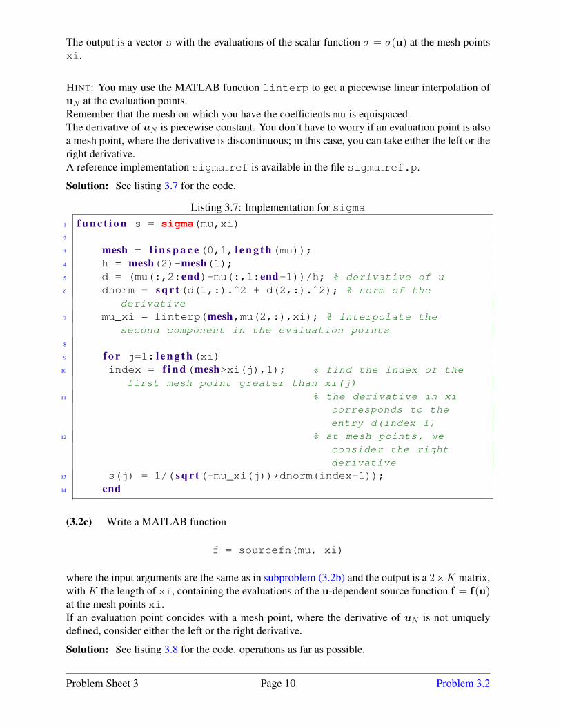
Solution: See listing 3.7 for the code.

Listing 3.7: Implementation for sigma1 f u n c t i o n s = sigma(mu,xi)2

3 mesh = l i n s p a c e(0,1, l e n g t h(mu));4 h = mesh(2)-mesh(1);5 d = (mu(:,2:end)-mu(:,1:end-1))/h; % derivative of u

6 dnorm = s q r t(d(1,:).ˆ2 + d(2,:).ˆ2); % norm of the

derivative

7 mu_xi = linterp(mesh,mu(2,:),xi); % interpolate the

second component in the evaluation points

8

9 f o r j=1: l e n g t h(xi)10 index = f i n d(mesh>xi(j),1); % find the index of the

first mesh point greater than xi(j)

11 % the derivative in xi

corresponds to the

entry d(index-1)

12 % at mesh points, we

consider the right

derivative

13 s(j) = 1/( s q r t(-mu_xi(j))*dnorm(index-1));14 end

(3.2c) Write a MATLAB function

f = sourcefn(mu, xi)

where the input arguments are the same as in subproblem (3.2b) and the output is a 2×K matrix,with K the length of xi, containing the evaluations of the u-dependent source function f = f(u)at the mesh points xi.If an evaluation point concides with a mesh point, where the derivative of uN is not uniquelydefined, consider either the left or the right derivative.

Solution: See listing 3.8 for the code. operations as far as possible.

Problem Sheet 3 Page 10 Problem 3.2

Listing 3.8: Implementation for sourcefn1 f u n c t i o n f = sourcefn(mu,xi)2

3 M = l e n g t h(mu)-1;4 mesh = l i n s p a c e(0,1, l e n g t h(mu));5 h = mesh(2)-mesh(1);6 d = (mu(:,2:end)-mu(:,1:end-1))/h; % derivative of u

7 dnorm = s q r t(d(1,:).ˆ2 + d(2,:).ˆ2); % norm of the

derivative

8 mu_xi = linterp(mesh,mu(2,:),xi);9

10 f(1,:)= z e r o s(1, l e n g t h(xi));11

12 f o r j=1: l e n g t h(xi)13 index = f i n d(mesh>xi(j),1); % find the index of the

first mesh point greater than xi(j)

14 % the derivative in xi

corresponds to the entry

d(index-1)

15 % at mesh points, we

consider the right

derivative

16 f(2,j) = dnorm(index-1)/(2* s q r t(-mu_xi(j))*mu_xi(j));17 end

(3.2d) Implement a MATLAB function

t = traveltime (mu)

which accepts as input the vector mu as in (3.2b), and returns the approximate value of the func-tional

J(uN) =

∫ 1

0

∥u′N(ξ)∥√

−(uN)2(ξ)dξ (3.2.4)

representing the time needed to go from u(0) to u(1) along the curve uN .

For the computation of the integral in (3.2.4), use the midpoint rule (see [NPDE, Eq. (1.5.77)]).Note that the trapezoidal rule would be inappropriate because of the singularity of the functionalat the origin.

HINT: A reference implementation traveltime ref is available in the file traveltime ref.p.

Solution: See listing 3.9 for the code.

Listing 3.9: Implementation for traveltime1 f u n c t i o n t = traveltime(mu)2

Problem Sheet 3 Page 11 Problem 3.2

3 mesh = l i n s p a c e(0,1, l e n g t h(mu));4 h = mesh(2)-mesh(1);5 d = (mu(:,2:end)-mu(:,1:end-1))/h;6 dnorm = s q r t(d(1,:).ˆ2 + d(2,:).ˆ2);7 % TRAPEZOIDAL RULE

8 % mu2 = mu(2,:);

9 % t =

sum((dnorm(1:end-1)+dnorm(2:end))./(sqrt(-mu2(2:(end-1)))))+...

10 % ...+dnorm(end)/sqrt(-mu2(end));

11 % if abs(mu2(1))>eps

12 % t = t+dnorm(1)/sqrt(-mu2(1));

13 % end

14 % MIDPOINT RULE

15 xi = h/2:h:(1-h/2);16 mu_xi = linterp(mesh,mu(2,:),xi);17 t = sum(dnorm./( s q r t(-mu_xi)))*h;

(3.2e) Proceeding as in [NPDE, § 1.5.82], the discretization of (3.2.3) leads to a nonlinearsystem of equations of the form(

R(µ) 00 R(µ)

)µ =

(φ1(µ)φ2(µ)

), (3.2.5)

with R(µ) ∈ RM−1,M−1 and φi(µ) ∈ RM−1. Write a MATLAB function

R = Rmat(mu)

such that, given the coefficients µ = mu in input (as in subproblem (3.2a)), returns the matrix R= R(µ).For the evaluation of the integrals, use the midpoint rule [NPDE, Eq. (1.5.77)].

HINT: Compute the matrix including also the rows and columns referring to the two basis func-tions for the offset function. In this way, your matrix R will have dimensions (M +1)× (M +1).Then, in subproblem (3.2g), where you will have to solve the linear system, you have to considerjust the entries relative to the inner nodes (i.e. you have to exclude the first and last columns androws of R). The reason for doing this is that with such R it will be easier, in subproblem (3.2g), tomodify the right hand side to take into account the boundary conditions.A reference implementation R ref is available in the file R ref.p.

Solution: See listing 3.10 for the code.

Listing 3.10: Implementation for Rmat1 f u n c t i o n R = Rmat(mu)2

3 mesh = l i n s p a c e(0,1, l e n g t h(mu));4 h = mesh(2)-mesh(1);5 xi = h/2:h:(1-h/2); % midpoints, where we will evaluate

sigma

Problem Sheet 3 Page 12 Problem 3.2

6 M = l e n g t h(mu)-1;7 % Computation of the r_j

8 s = sigma(mu,xi);9 r = s./h;

10

11 % Assemble tridiagonal matrix R

12 R = g a l l e r y(’tridiag’,[-r(1), -r(2:M-1),-r(M)],[r(1),r(1:M-1)+r(2:M), r(M)],[-r(1), -r(2:M-1), -r(M)]);

(3.2f) Write a MATLAB function

phi = rhs(mu)

which, given the coefficients mu in input, returns as output the right hand side vector from (3.2.5)

φ(µ) =

(φ1(µ)φ2(µ)

)∈ R2M−2 . (3.2.6)

For integration, consider the composite trapezoidal quadrature rule [NPDE, Eq. (1.5.72)]. At theorigin (where the source function is singular), consider the integrand to be zero.HINT: A reference implementation rhs ref is available in the file rhs ref.p.

Solution: See listing 3.11 for the code.

Listing 3.11: Implementation for rhs1 f u n c t i o n phi = rhs(mu)2

3 mesh = l i n s p a c e(0,1, l e n g t h(mu));4 h = mesh(2)-mesh(1);5 % TRAPEZOIDAL RULE

6 xxi = h:h:(1-h);7 phi =

(sourcefn(mu,xxi(1:end))+sourcefn(mu,xxi(1:end)))*h/2;8 % MIDPOINT RULE: DOESN’T WORK!

9 % xi = h/2:h:(1-h/2);

10 % sourcefn(mu,xxi); % for debugging

11 % 2*sourcefn(mu,xxi) % for debugging

12 % source = sourcefn(mu,xi);

13 % source(:,1:end-1) + source(:,2:end) % for debugging

14 % phi = source(:,1:end-1)*h/2 + source(:,2:end)*h/2;

(3.2g) The nonlinear system (3.2.6) can be solved by fixed point iteration. In this way, anapproximate solution is computed solving, at each iteration, a linear system of equations (see[NPDE, § 1.5.82], [NPDE, Code 1.5.92]).Implement a MATLAB function

mufinal = solvebrachlin(mu0, tol)

Problem Sheet 3 Page 13 Problem 3.2

to compute the approximate solution (i.e. the coefficients mufinal with respect to the basisfunctions) using the fixed point iteration.The input arguments are the initial guess mu0 and the tolerance tol for the relative error in thefixed point iteration algorithm (see [NPDE, Code 1.5.92], line 41).For each iteration, plot the shape of the curve (see [NPDE, Code 1.5.92], lines 19-22).Plot the travel time as defined in subproblem (3.2d) with respect to the number of iteration steps.Remark: Remember to take into account the boundary conditions.

HINT: The solution should look like the cycloid

u(ξ) =

(πξ − sin(πξ)cos(πξ)− 1

), 0 ≤ ξ ≤ 1 , (3.2.7)

that was shown in the previous assignment to be a strong solution.A reference implementation solvebrachlin ref is available in the file solvebrachlin ref.p.

Solution: See listing 3.12 for the code.

Listing 3.12: Implementation for solvebrachlin1 f u n c t i o n [mu_new,figsol] = solvebrachlin(init_guess,tol)2 % M intervals, M-1 interior nodes

3 M = l e n g t h(init_guess)-1;4 h= 1/M; %meshwidth

5

6 figsol = f i g u r e; hold on;7 maxiter=10000;8 mu_new = init_guess;9 t = [];

10 f o r k=1:maxiter11 mu = mu_new;12 % Plot shape of string

13 p l o t(mu(1,:), mu(2,:),’--g’); drawnow;14 t i t l e ( s p r i n t f(’M = %d, iteration #%d’, M,k));15 x l a b e l(’{\bf x_1}’); y l a b e l(’{\bf x_2}’);16 t = [t; traveltime(mu)];17

18 R = Rmat(mu);19 % Computation of right hand side

20 phi = rhs(mu);21 phi1 = phi(1,:);22 phi2 = phi(2,:);23

24 % Modify right hand side to take in account to the offset

function

25 phi1(1)= phi1(1) - R(2,1)*mu(1,1);26 phi1(M-1) = phi1(M-1) -R(M,M+1)*mu(1,end);27 phi2(1) = phi2(1) - R(2,1)*mu(2,1);28 phi2(M-1) = phi2(M-1) -R(M,M+1)*mu(2,end);29

Problem Sheet 3 Page 14 Problem 3.2

30 % Solve linear system and compute new iterate

31 mu_new = [mu(:,1),[(R((2:end-1),(2:end-1))\phi1’)’;32 (R((2:end-1),(2:end-1))\phi2’)’],mu(:,end)];33 % Check simple termination criterion for fixed point

iteration.

34 i f (norm(mu_new - mu,’fro’) < tol*norm(mu_new,’fro’)/M)35 p l o t(mu_new(1,:),mu_new(2,:),’r’);36 xi = l i n s p a c e(0,1);37 p l o t(pi*xi- s i n(pi*xi),cos(pi*xi)-1,’b’);38 break;39 end40

41 end42 f i g u r e43 p l o t(t);

The solution for M=16, with straight line as initial guess, should look like the following:

(3.2h) The fixed point iteration algorithm converges quite slowly to the approximate solution.To improve this, we use nested iterations:

a) start from an initial guess mu0 and an initial coarse mesh mesh0 and compute the solutionmu1;

b) consider the mesh mu1 obtained from mu0 inserting the midpoints of the interval as meshpoints (thus doubling the number of mesh points) and compute the solution mu2 consider-ing mu1 as initial guess;

c) repeat point b) iteratively until the desired final meshwidth level L is reached.

In point b), to get the initial guess, one has to extend a piecewise linear function defined on acoarser grid to a finer nested grid. To achieve this, piecewise linear interpolation can be used.

Problem Sheet 3 Page 15 Problem 3.2

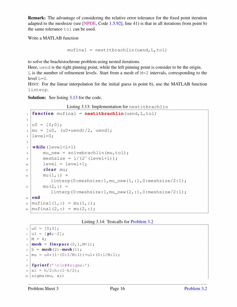
Remark: The advantage of considering the relative error tolerance for the fixed point iterationadapted to the meshsize (see [NPDE, Code 1.5.92], line 41) is that in all iterations from point b)the same tolerance tol can be used.

Write a MATLAB function

mufinal = nestitbrachlin(uend,L,tol)

to solve the brachistochrone problem using nested iterations.Here, uend is the right pinning point, while the left pinning point is consider to be the origin.L is the number of refinement levels. Start from a mesh of M=2 intervals, corresponding to thelevel L=0.HINT: For the linear interpolation for the initial guess in point b), use the MATLAB functionlinterp.

Solution: See listing 3.13 for the code.

Listing 3.13: Implementation for nestitbrachlin1 f u n c t i o n mufinal = nestitbrachlin(uend,L,tol)2

3 u0 = [0;0];4 mu = [u0, (u0+uend)/2, uend];5 level=0;6

7 whi le(level<L+1)8 mu_new = solvebrachlin(mu,tol);9 meshsize = 1/(2ˆ(level+1));

10 level = level+1;11 c l e a r mu;12 mu(1,:) =

linterp(0:meshsize:1,mu_new(1,:),0:meshsize/2:1);13 mu(2,:) =

linterp(0:meshsize:1,mu_new(2,:),0:meshsize/2:1);14 end15 mufinal(1,:) = mu(1,:);16 mufinal(2,:) = mu(2,:);

Listing 3.14: Testcalls for Problem 3.21 u0 = [0;0];2 u1 = [pi;-2];3 M = 4;4 mesh = l i n s p a c e(0,1,M+1);5 h = mesh(2)-mesh(1);6 mu = u0*(1-(0:1/M:1))+u1*(0:1/M:1);7

8 f p r i n t f(’\n\n##sigma:’)9 xi = h/2:h:(1-h/2);

10 sigma(mu, xi)

Problem Sheet 3 Page 16 Problem 3.2

11

12 f p r i n t f(’\n\n##sourcefn:’)13 xxi = h:h:(1-h);14 sourcefn(mu,xxi)15

16 f p r i n t f(’\n\n#traveltime:’)17 traveltime(mu)18

19 f p r i n t f(’\n\n##Rmat:’)20 Rmat(mu)21

22 f p r i n t f(’\n\n##rhs:’)23 rhs(mu)24

25 f p r i n t f(’\n\n##solvebrachlin:’)26 solvebrachlin(mu,10ˆ(-5))27

28 f p r i n t f(’\n\n##nestitbrachlin:’)29 nestitbrachlin([pi;-2],3,10ˆ(-5))

Listing 3.15: Output for Testcalls for Problem 3.21 >> test_call_fem2

3 ##sigma:4 ans =5

6 0.5370 0.3101 0.2402 0.20307

8 ##sourcefn:9 ans =

10

11 0 0 012 -5.2668 -1.8621 -1.013613

14 #traveltime:15 ans =16

17 4.473718

19 ##Rmat:20 ans =21

22 (1,1) 2.148123 (2,1) -2.148124 (1,2) -2.148125 (2,2) 3.388326 (3,2) -1.240227 (2,3) -1.240228 (3,3) 2.2009

Problem Sheet 3 Page 17 Problem 3.2

29 (4,3) -0.960730 (3,4) -0.960731 (4,4) 1.772632 (5,4) -0.811933 (4,5) -0.811934 (5,5) 0.811935

36 ##rhs:37 ans =38

39 0 0 040 -1.3167 -0.4655 -0.253441

42 ##solvebrachlin:43 ans =44

45 0 0.3114 1.0169 1.9977 3.141646 0 -0.6794 -1.3570 -1.8269 -2.000047

48 ##nestitbrachlin:49 ans =50

51 Columns 1 through 952

53 0 0.0510 0.1019 0.2179 0.3339 0.49940.6650 0.8683 1.0717

54 0 -0.1679 -0.3358 -0.5287 -0.7215 -0.9031-1.0847 -1.2425 -1.4002

55

56 Columns 10 through 1757

58 1.3040 1.5364 1.7906 2.0447 2.3145 2.58432.8629 3.1416

59 -1.5280 -1.6558 -1.7500 -1.8442 -1.9022 -1.9602-1.9801 -2.0000

Problem 3.3 Spline Collocation Method[NPDE, Section 1.5.3.2] introduces the spline collocation method for 2-point boundary value problemsbased on natural cubic splines, see [NPDE, Def. 1.5.116]. In this problem we consider the simple BVP

−d2u

dx2= f(x) in [0, 1], u(0) = u(1) = 0, (3.3.1)

f ∈ C0([0, 1]), and its cubic spline collocation discretization based on the knot set

T := {jh}Mj=0, h := 1/M, M ∈ N, (3.3.2)

and on the set of collocation nodes {jh}M−1j=1 .

(3.3a) Refresh your knowledge of the basic idea of discretization by collocation as explained in thebeginning of [NPDE, Section 1.5.3].

Problem Sheet 3 Page 18 Problem 3.3

(3.3b) Any cubic spline s ∈ S3,T has the local monomial representation

s(x) = ai(x− xi−1)3 + bi(x− xi−1)

2 + ci(x− xi−1) + di, xi−1 < x < xi, i = 1, . . . ,M, (3.3.3)

with coefficients ai, bi, ci, di ∈ R. This local monomial representation will be used in the sequel.

Denote fi := f(xi), i = 0, . . . ,M .

Show that the collocation conditions [NPDE, Eq. (1.5.100)] imply the following formulas

ai =fi−1 − fi

6h, i = 1, . . . ,M, (3.3.4a)

b1 = 0 (3.3.4b)

bi = −12fi−1, i = 2, . . . ,M, (3.3.4c)

for the coefficients of the local monomial representation of the spline solving the collocation equations (inthe fist equation we have set fM := s′′(1) = 0).

Solution: A natural cubic spline s : [0, 1] → R satisfies

(i) s ∈ C2([0, 1]),

(ii) s∣∣[xj−1,xj ]

∈ P3(R),

(iii) s′′(0) = s′′(1) = 0.

With (ii) we know that for xi−1 ≤ x ≤ xi, i = 1, . . . ,M we have

s(x) = ai(x− xi−1)3 + bi(x− xi−1)

2 + ci(x− xi−1) + di,

s′(x) = 3ai(x− xi−1)2 + 2bi(x− xi−1) + ci,

s′′(x) = 6ai(x− xi−1) + 2bi.

Since −s′′(xi−1) = f(xi−1) we have .

2bi = −f(xi−1) = −fi−1 ⇒ bi =1

2fi−1, i = 2, . . . ,M,

and b1 = 0 since s′′(0) = 0. We also have for −s′′(xi) = f(xi) that

−6aih− fi−1 = fi ⇒ ai =fi−1 − fi

6hi = 1, . . . ,M.

(3.3c) The equations (3.3.4) are too few to determine all unknown coefficients. To obtain further equa-tions, use the continuity conditions for the “zeroth” and first derivative of a cubic spline, the collocationand boundary conditions at x = 0 and x = 1, and the relationships (3.3.4) to establish

d1 = 0 (3.3.5a)

di+1 − 2di + di−1 = −h2

6(fi + 4fi−1 + fi−2), 2 ≤ i ≤ M − 1, (3.3.5b)

c2 − c1 = −h

2f1, (3.3.5c)

ci+1 − ci = −h

2(fi + fi−1), 2 ≤ i ≤ M − 1, (3.3.5d)

cMh+ dM =h2

3fM−1, (3.3.5e)

cM−1h+ dM−1 − dM =h2

6(2fM−2 + fM−1). (3.3.5f)

Problem Sheet 3 Page 19 Problem 3.3

HINT: Recall the formulas for interpolating natural cubic splines from [NCSE, Sect. 3.8.1].

Solution: Since s′(x) is continuous we have

ci+1 = s′(xi) = 3aih2 + 2bih+ ci

= 3fi−1 − fi

6hh2 − 2

fi−1

2h+ ci

= −fi + fi−1

2h+ ci.

Therefore ci+1 − ci = −fi+fi−1

2 h for i = 2, . . . ,M − 1 and ci+1 − ci = −fi2 h for i = 1.

Furthermore, since s(x) is continuous, we obtain

di = s(xi) = ai−1h3 + bi−1h

2 + ci−1h+ di−1,⇒ di+1 − di = aih

3 + bih2 + cih;

this implies

⇒ di+1 − 2di + di−1 =h3(fi−1 − fi − fi−2 + fi−1

6h

)+ h2

(−fi−1 + fi−2

2

)+

h2

2(−fi−1 − fi−2) =

=− h2

6(fi + 4fi−1 + fi−2),

for i = 2, . . . ,M − 1, and

cM−1h+ dM−1 − dM = −aM−1h3 − bM−1h

2 =h2

6(2fM−2 + fM−1).

Additionally, the boundary conditions s(0) = s(1) imply, respectively, d1 = 0 and

cMh+ dM =h2

3fM−1.

(3.3d) Write a MATLAB function

function [a,b,c,d] = natcubsplinecoll(M,f)

that computes the local monomial expansion coefficients of the natural cubic spline collocation solution of(3.3.1) with node set (3.3.2). These coefficients are to be returned in the row vectors a, b, c, d of lengthM . The argument f is a handle to the (continuous) right hand side function f .

Solution: See Listing 3.16.

Listing 3.16: Code for subproblem (3.3d).1 f u n c t i o n [a,b,c,d] = natcubsplinecoll(M,f)2

3 % Computes the coefficients in the monomial expansion of the splinefor

4 % equispace knots5 % INPUT:6 % M = number of intervals7 % f = FHandle to right-hand side8 % OUTPUT:

Problem Sheet 3 Page 20 Problem 3.3

9 % column vectors of coefficients in the monomial expansion10

11 h = 1/M;12 x = l i n s p a c e(0,1,M+1);13 fval = f(x);14 fval = fval(:);15 a = (fval(1:end-1)-fval(2:end))/(6*h);16 b = [0; -fval(2:end-1)/2];17 A11 = diag([-ones(M-1,1);h])+diag(ones(M-1,1),1);18 A12 = z e r o s(M,M);19 A12(end,end) = 1;20 A21 = z e r o s(M,M);21 A21(end,end-1) = h;22 A22 =

diag([1;-2*ones(M-2,1);-1])+diag([0;ones(M-2,1)],1)+diag([ones(M-2,1);1],-1);23 A = [A11 A12; A21 A22];24 RHS = z e r o s(2*M,1);25 RHS(1:M-1)=(fval(2:end-1)+fval(1:end-2))*(-h/2);26 RHS(M) = fval(end-1)*hˆ2/3;27 RHS(M+1) = 0;28 RHS(M+2:end-1) = -hˆ2/6*(fval(3:M)+4*fval(2:M-1)+fval(1:M-2));29 RHS(end) = hˆ2/6*(2*fval(M-1)+fval(M));30 res = A\RHS;31 c = res(1:M);32 d = res(M+1:end);

(3.3e) Plot the approximate solution of (3.3.1) with f(x) = sin(2πx) obtained by natural cubic splinecollocation on an equidistant node set (3.3.1) with M = 5, 10, 20.

Solution: See Listing 3.17.

Listing 3.17: Code for subproblem (3.3e).1 f = @(x) s i n(2*pi.*x(:));2

3 M = 20;4 [a, b, c, d]=natcubsplinecoll(M,f);5 x = l i n s p a c e(0,1,M+1);6 xx = l i n s p a c e(0,1,4*M+1);7 yy = [];8 f o r i=1:M9 yval = a(i)*(xx((i-1)*4+1:i*4+1)-x(i)).ˆ3 +

b(i)*(xx((i-1)*4+1:i*4+1)-x(i)).ˆ2 +c(i)*(xx((i-1)*4+1:i*4+1)-x(i)) + d(i);

10 yy = [yy(1:end-1) yval];11 end12

13 p l o t(xx,yy,’o’)

For M = 20 we obtain the plot shown in Figure 3.4.

Problem Sheet 3 Page 21 Problem 3.3

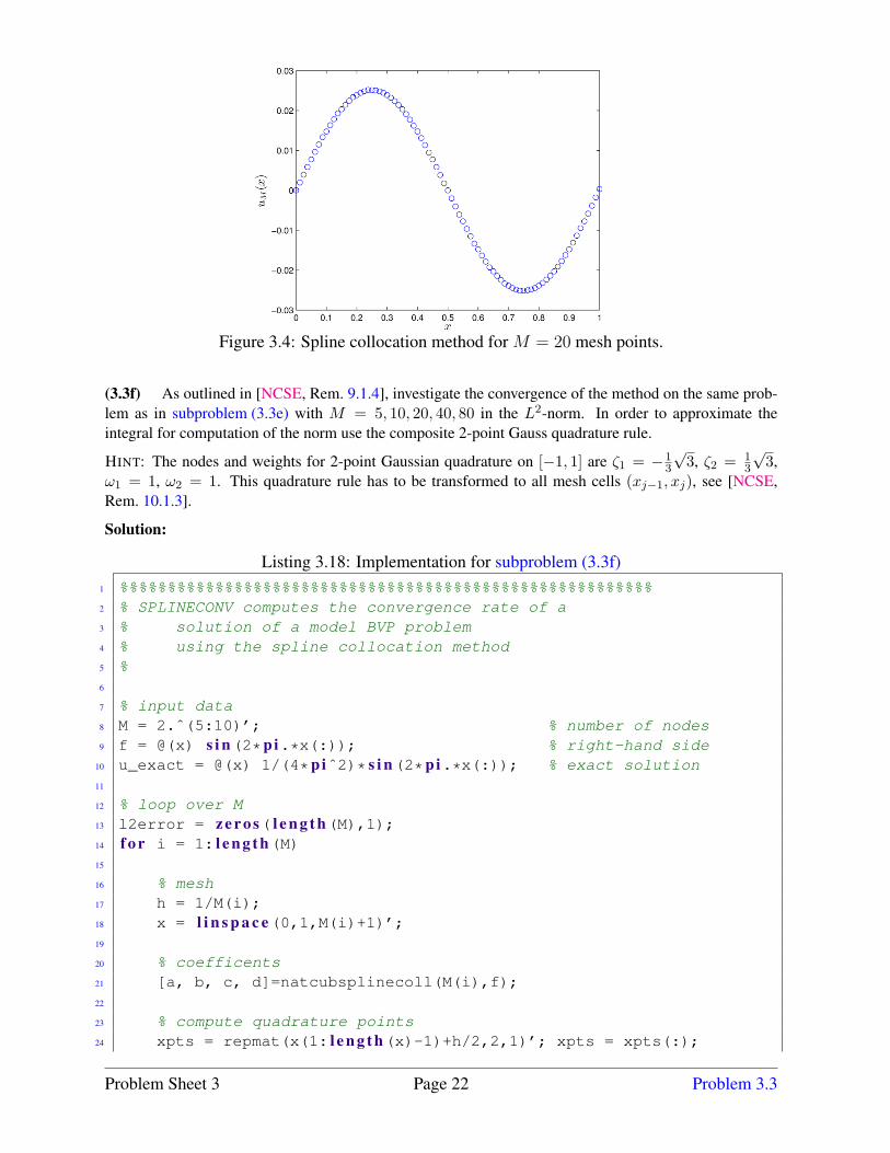
Figure 3.4: Spline collocation method for M = 20 mesh points.

(3.3f) As outlined in [NCSE, Rem. 9.1.4], investigate the convergence of the method on the same prob-lem as in subproblem (3.3e) with M = 5, 10, 20, 40, 80 in the L2-norm. In order to approximate theintegral for computation of the norm use the composite 2-point Gauss quadrature rule.

HINT: The nodes and weights for 2-point Gaussian quadrature on [−1, 1] are ζ1 = −13

√3, ζ2 = 1

3

√3,

ω1 = 1, ω2 = 1. This quadrature rule has to be transformed to all mesh cells (xj−1, xj), see [NCSE,Rem. 10.1.3].

Solution:

Listing 3.18: Implementation for subproblem (3.3f)1 %%%%%%%%%%%%%%%%%%%%%%%%%%%%%%%%%%%%%%%%%%%%%%%%%%%%%%%%2 % SPLINECONV computes the convergence rate of a3 % solution of a model BVP problem4 % using the spline collocation method5 %6

7 % input data8 M = 2.ˆ(5:10)’; % number of nodes9 f = @(x) s i n(2*pi.*x(:)); % right-hand side

10 u_exact = @(x) 1/(4*piˆ2)* s i n(2*pi.*x(:)); % exact solution11

12 % loop over M13 l2error = z e r o s( l e n g t h(M),1);14 f o r i = 1: l e n g t h(M)15

16 % mesh17 h = 1/M(i);18 x = l i n s p a c e(0,1,M(i)+1)’;19

20 % coefficents21 [a, b, c, d]=natcubsplinecoll(M(i),f);22

23 % compute quadrature points24 xpts = repmat(x(1: l e n g t h(x)-1)+h/2,2,1)’; xpts = xpts(:);

Problem Sheet 3 Page 22 Problem 3.3

25 gqpts = repmat([-1;1]/ s q r t(3),1,M(i))’*h/2; gqpts = gqpts(:) +xpts;

26 gqpts = s o r t(gqpts);27

28 % compute solution in quadrature points29 u = [];30 f o r j=1:M(i)31 uval = a(j)*(gqpts((j-1)*2+1:j*2)-x(j)).ˆ3 +

b(j)*(gqpts((j-1)*2+1:j*2)-x(j)).ˆ2 +c(j)*(gqpts((j-1)*2+1:j*2)-x(j)) + d(j);

32 u = [u; uval];33 end34

35 % compute error36 l2error(i) = s q r t(sum(h/2*(u-u_exact(gqpts)).ˆ2));37 end38

39 % compute convergence rate40 p = p o l y f i t( l o g(M), l o g(l2error),1);41 s = p(1);42 f p r i n t f(’Convergence rate s = %2.4f\n’,abs(s));43

44 % plot convergence rate45 f i g u r e(1)46 h = axes;47 l o g l o g(M,l2error,’bo-’)48 hold on;49 add_Slope(gca,’NorthEast’,p(1));50 gr id on51 s e t(h,’FontSize’,14);52 x l a b e l(’M’)53 y l a b e l(’Lˆ2-error’)54 %print -depsc splineconv.eps

We obtain the optimal convergence rate s = 2 as shown in Figure 3.5.

Listing 3.19: Testcalls for Problem 3.31

2 f p r i n t f(’\n\n##natcubsplinecoll:’)3

4 f = @(x) s i n(2*pi.*x(:));5 M = 5;6 [a, b, c, d]=natcubsplinecoll(M,f)

Listing 3.20: Output for Testcalls for Problem 3.31 >> test_call2

3 ##natcubsplinecoll:4 a =

Problem Sheet 3 Page 23 Problem 3.3

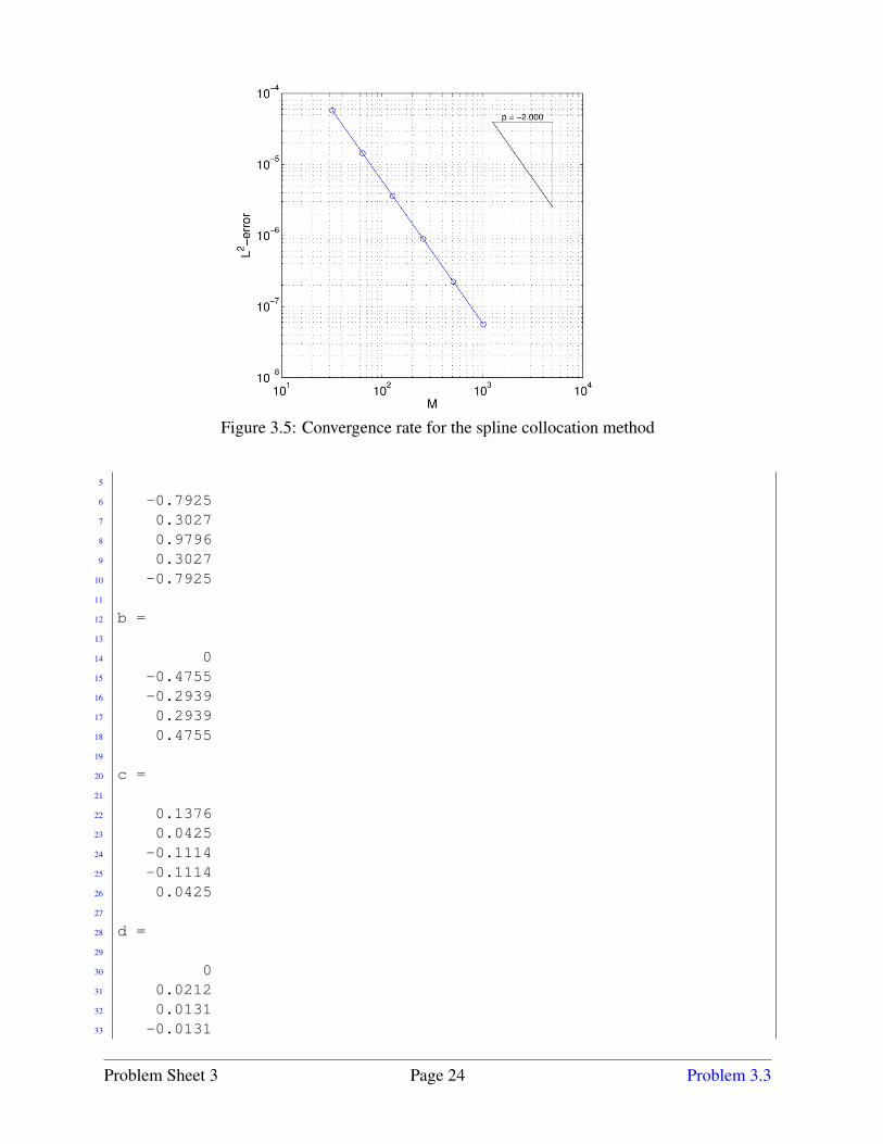
Figure 3.5: Convergence rate for the spline collocation method

5

6 -0.79257 0.30278 0.97969 0.3027

10 -0.792511

12 b =13

14 015 -0.475516 -0.293917 0.293918 0.475519

20 c =21

22 0.137623 0.042524 -0.111425 -0.111426 0.042527

28 d =29

30 031 0.021232 0.013133 -0.0131

Problem Sheet 3 Page 24 Problem 3.3

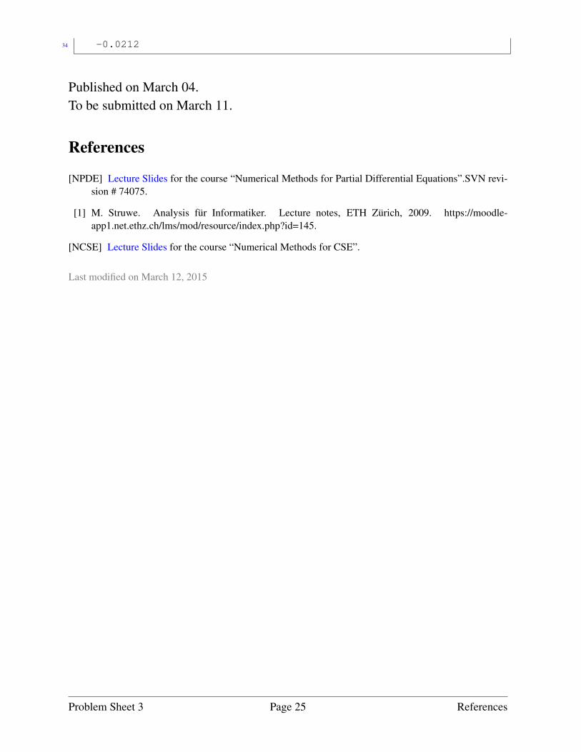
34 -0.0212

Published on March 04.To be submitted on March 11.

References

[NPDE] Lecture Slides for the course “Numerical Methods for Partial Differential Equations”.SVN revi-sion # 74075.

[1] M. Struwe. Analysis fur Informatiker. Lecture notes, ETH Zurich, 2009. https://moodle-app1.net.ethz.ch/lms/mod/resource/index.php?id=145.

[NCSE] Lecture Slides for the course “Numerical Methods for CSE”.

Last modified on March 12, 2015

Problem Sheet 3 Page 25 References