Numerical Methods for Option Pricing

Kimiya MinoukadehEcole Polytechnique

M2 Mathématiques Appliquées, OJME

Prof: Olivier Pironneau

Agenda• Introduction to Monte-Carlo method

• Heston stochastic volatility model using M-C

• Basket option using Monte-Carlo

• Accuracy of Monte-Carlo methods

• Variance Reduction methods

• Conclusion

Monte-Carlo Method I

• Based on the expectation of a random variable X, given N samples {X1,X2,…,XN}

• Price of a European Call option is therefore calculated as

where: is the ith estimate of the stock price at time T, the time of maturation, r is the risk free interest rate and K is the strike price.

Monte-Carlo Method II

• The stock price St follows the stochastic differentialEquation (SDE)

where

• is the drift term

• is the volatility

•

Agenda• Introduction to Monte-Carlo method

• Heston stochastic volatility model using M-C

• Basket option using Monte-Carlo

• Accuracy of Monte-Carlo methods

• Variance Reduction methods

• Conclusion

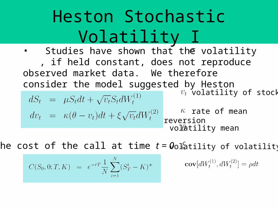
• Studies have shown that the volatility , if held constant, does not reproduce observed market data. We therefore consider the model suggested by Heston

Heston Stochastic Volatility I

volatility of stock

rate of mean reversion

volatility mean

volatility of volatilityThe cost of the call at time t = 0

• Results are consistent with the a priori lower bounds known for call options.

Heston stochastic volatility II

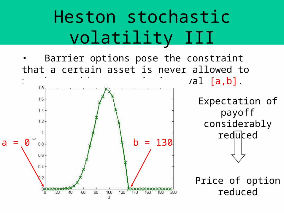
• Barrier options pose the constraint that a certain asset is never allowed to reach outside a certain interval [a,b].

Heston stochastic volatility III

b = 130 a = 0

Expectation of payoff considerably

reduced

Price of option reduced

Agenda• Introduction to Monte-Carlo method

• Heston stochastic volatility model using M-C

• Basket option using Monte-Carlo

• Accuracy of Monte-Carlo methods

• Variance Reduction methods

• Conclusion

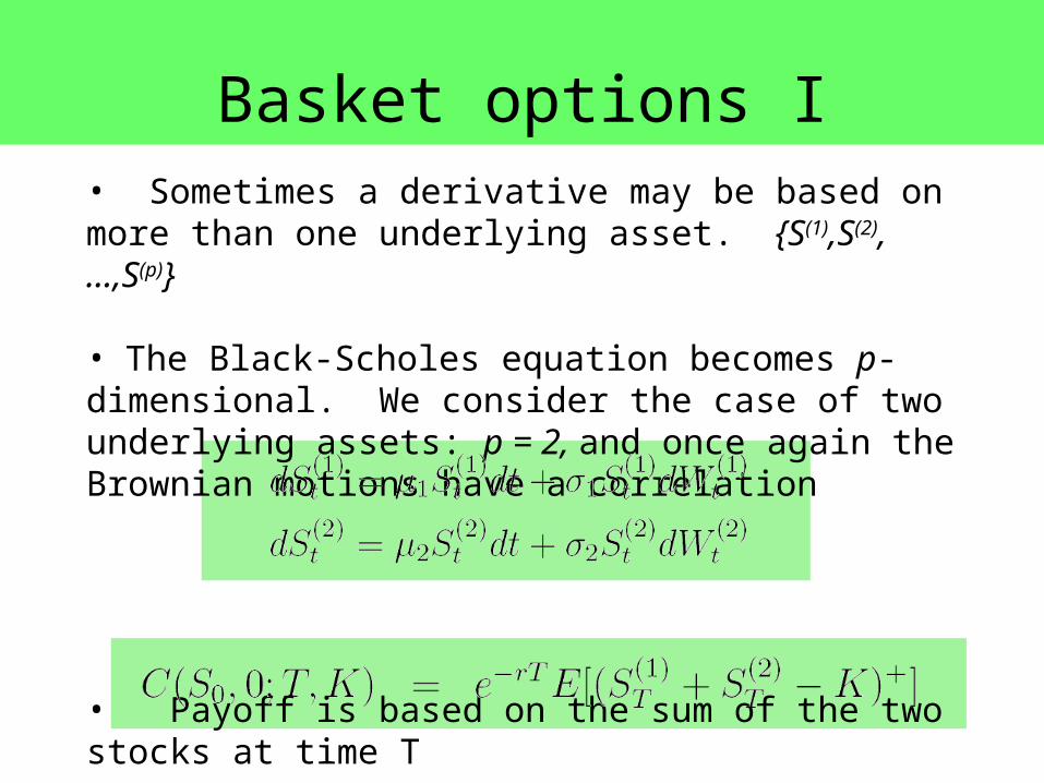
• Sometimes a derivative may be based on more than one underlying asset. {S(1),S(2),…,S(p)}

• The Black-Scholes equation becomes p-dimensional. We consider the case of two underlying assets: p = 2, and once again the Brownian motions have a correlation

• Payoff is based on the sum of the two stocks at time T

Basket options I

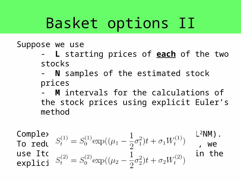
Suppose we use- L starting prices of each of the two stocks- N samples of the estimated stock prices- M intervals for the calculations of the stock prices using explicit Euler’s method

Complexity of the program would be O(L2NM). To reduce this by a factor M to O(L2N), we use Ito’s Lemma with Yi = log(S(i)) to obtain the explicit solution to the SDE

Basket options II

Basket options III

By using the explicit solution we can observe that we get desirable results, accuracy similar to using the Explicit Euler’s method, however time performance improved dramatically.

ERROR ANALYSISTIME PERFORMANCE

• Letting K = K1 + K2 for the respective quasi strike prices of stocks S(1) and S(2), we observe the following results

Basket options IV

By choosing S0(1) = K1 = 100,

we observe that results resemble that of a standard European call option with one underlying asset

Agenda• Introduction to Monte-Carlo method

• Heston stochastic volatility model using M-C

• Basket option using Monte-Carlo

• Accuracy of Monte-Carlo methods

• Variance Reduction methods

• Conclusion

The central limit theorem shows that the accuracy of the Monte-Carlo method is controlled by

Accuracy of Monte-Carlo method

Thus to halve the error we would need to quadruple the number of samples N used in the Monte-Carlo simulation.

Agenda• Introduction to Monte-Carlo method

• Heston stochastic volatility model using M-C

• Basket option using Monte-Carlo

• Accuracy of Monte-Carlo methods

• Variance Reduction methods

• Conclusion

IDEA: Reduce the variance of the random process X.

For an independent random process Y, we note that

The variance is then given by

therefore we have

Variance Reduction Methods I

Need to choose a random variable Y such that it is closely correlated with X.

We adapt a method suggested by P. Pellizzari [1] for variance reduction of basket options

Variance Reduction Methods II

[1] P. Pellizzari. Efficient Monte-Carlo pricing of basket options. Finance, EconWPA, 1998

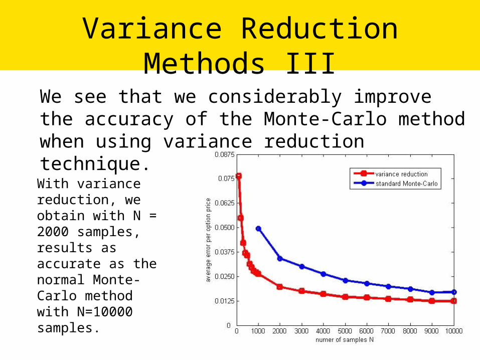
We see that we considerably improve the accuracy of the Monte-Carlo method when using variance reduction technique.

Variance Reduction Methods III

With variance reduction, we obtain with N = 2000 samples, results as accurate as the normal Monte-Carlo method with N=10000 samples.

Agenda• Introduction to Monte-Carlo method

• Heston stochastic volatility model using M-C

• Basket option using Monte-Carlo

• Accuracy of Monte-Carlo methods

• Variance Reduction methods

• Conclusion

Conclusion

The Monte-Carlo method is intuitive and extremely easy to implement

It can be used to calculate call prices when an analytic solution of a PDE does not exist

Data is consistent with observed data

For well estimated expectations we need many sample simulations. To double accuracy, number of samples must quadruple.

IMPROVEMENT: When analytic solutions do not exist and we are obliged to use Monte-Carlo methods, variance reduction can improve the performance of the calculation.