NUMERICAL METHODS FOR DETERMINING THE … · successfully in helicopter rotor dynamics and...

Camp. & Maths. withAppls. VoL 12A. No. t. pp. 131-148. 1986 0097-4qg3/Sb $3.1X)~-.00 Pnnted in Great Britain. ¢ Iq86 Pergamon Pre,s Ltd

N U M E R I C A L METHODS FOR D E T E R M I N I N G THE STABILITY AND RESPONSE OF PERIODIC SYSTEMS

WITH APPLICATIONS TO HELICOPTER ROTOR D Y N A M I C S AND AEROELASTICITY

PERETZ P. FRIEDMANN Mechanical. Aerospace and Nuclear Engineering Department. University of California

at Los Angeles. Los Angeles. CA 90024. U.S.A.

Abstract - -This paper reviews and extends some recently developed numerical techniques for analyzing the stability, linear response and nonlinear response of periodic systems, which are governed by ordinary differential equations with periodic coefficients. The main emphasis is on applications aimed at rotor blade aeroelastic stability and response calculations in forward flight. First Floquet theory, is briefly reviewed and numerically efficient methods for evaluating the transition matrix at the end of one period are described. Next the numerical treatment of the linear response problem is discussed. Finally the numerical solution of the nonlinear response problem is treated using quasilinearization and periodic shooting. Applications illustrating numerical properties of the methods are described.

[A(~)] [C,l

[C(~, k)] [C(d/)l

i [/1

J K

[K(O)] k

[L(~)] [M]

{N,(O, y)}, {N,, d:. y, j,}

{qO)} [e(q,)l

[Q] JR]

$

[Sl, T t

{y} b.~O, k)}

[vo} {y,I

{z(~,)}

[A] k, A,

[¢(~. ~,,)] [¢A(T. 0)], [¢b,~(T. 0)]

(JOj

fl

NOMENCLATURE

periodic matrix constant matrix approximation of [A(O:)] over kth interval step function approximation to [A(~)] symbolic matrix representing linear damping effects complete nonlinear loading periodic shooting iteration index unit matrix number of terms used in the approximation of matrix exponential number of intervals into which T is divided symbolic matrix representing linear stiffness effects quasilinearization iteration index linear periodic matrix symbolic matrix representing linear inertia effects nonlinear parts of system in state space nonlinear state vector generalized coordinate vector. (n × l) periodic matrix used in Floquet theorem constant matrix constant matrix used in Floquet theorem index sensitivity matrix for periodic shooting, ith iteration common nondimensional period time state variable vector. (2n × I) approximate value of {y(d:)} value of state vector at beginning of period value of state vector at end of period integrated state at end of period for linear inhomogeneous periodic system with zero initial conditions excitation in the state space small quantity, error real part of characteristic exponent diagonal matrix containing characteristic exponents diagonal matrix containing characteristic multipliers characteristic exponent characteristic multiplier dummy variable transition matrix at nondimensional time for initial conditions give at ~b,, various approximations of [¢(T, 0)] at end of one period nondimcnsional time coordinate, also azimuth angle of blade ~b = fb measured from straight aft position imaginary part of characteristic exponent speed of rotation of rotor

131

132 PERETZ P. FRIED'qANN

Special Symbols [ ] square matrix

[ ] ~ inverse -~, = +~ - +~_, stepsize

( )R. ( )~ real and imaginary part o f a quantity d differentiation with respect to nondimensional time ( ) = - -

d+

I . I N T R O D U C T I O N

The equations of motion for a wide class of dynamical systems are mathematically represented by a system of ordinary differential equation with periodic coefficients. These equations can be either linear or nonlinear. Two basic problems associated with these systems are of significant engineering importance; the stability of such systems and their response under various kinds of excitation. In a previous paper[I] the efficient numerical treatment of linear periodic systems was discussed, in considerable detail, with an emphasis on stability problems. In Ref. 1 two numerically efficient methods for dealing with the stability of linear periodic systems ,~ere presented and applied to the classical parametrically excited beam problem, a helicopter rotor aeroelastic problem in forward flight and a ground resonance type of aeromechanical problem. The purpose of this paper is to briefly review some previous work on equations with periodic coefficients with applications to helicopter rotor dynamic problems and present a number of recently developed numerical methods which are applicable to the treatment of two important problems, namely (a) response of a linear periodic system under a periodic excitation and (b) response of a nonlinear periodic system under periodic excitation. These two mathematical problems occur frequently in rotary wing aeroelastic stability and response calculations[2] and their efficient numerical treatment has a central role in helicopter rotor dynamics, aeroelasticity and structural dynamics.

Although the main objective of the paper is to discuss methods which have been used successfully in helicopter rotor dynamics and aeroelasticity it is relevant to note that a vast amount of literature exists on various mathematical aspects of equations with periodic coefficients[3-8]. In addition to the mathematical interest in the subject a wide range of practical applications of periodic systems has generated significant research on this topic in various disciplines within engineering and applied science. The most notable of these is control system theory and network theory{9-11], dynamic stability problems in applied mechanics[12] and nonlinear oscillations[ 131.

A variety of helicopter rotor dynamic and aeroelastic problems in forward flight are governed by ordinary differential equations with periodic coefficients[2,14]. Therefore papers dealing with the mathematical and numerical treatment of equations with periodic coefficients as applied to helicopter rotor dynamic problems have appeared in the literature since the late 1940s. A complete review of these studies is beyond the scope of this paper, however, to provide a historical perspective, some of the more useful references, dealing with helicopter rotor dynamic problems, will be briefly mentioned. The first papers written on this subject were aimed at determining the stabili~ of rotor blade flapping motions at high advance ratios. A pioneering contribution to the subject was a paper by Horvay and Yuan[15] which was based on the rectangular ripple method. In the 1960s a number of papers were written on both the flapping as well as coupled flap-torsional dynamics in forward flight[16-191; however these papers were based on direct numerical integration of the equations of motion or Hill's method of infinite determinants[12] which are not as convenient for implementation on digital computers as later methods which are based on Floquet's theorem[3,6,10,11 ].

In 1970, Hall[20] was the first to recognize that Floquet theory combined with the state variable representation of the equations of motion (as used in control systems engineering) was the most effective technique for dealing with rotor blade stability problems. At the same time Gockel[21] emphasized the applicability of Floquet theory to the solution of variety of rotor dynamic problems and Peters and Hohenemser[22] applied the theory to the solution of the blade flapping stability problem in forward flight. Subsequently Floquet theory was applied to more complicated rotordynamic problems. Hammond used the theory to study the ground resonance problem of a helicopter with one blade damper inoperative[23]. Friedmann and

Numerical methods for determining the stability and response of periodic systems 133

Silverthorn applied the theory to the coupled flap-lag aeroelastic problem of a hingeless rotor blade in forward flight[24]. The treatment of these, somewhat more complicated, problems required improved numerical schemes for the computation of the transition matrix at the end of one period. Therefore, in both Refs. 23 and 24, improved numerical schemes for the calculation of the transition matrix at the end of one period were presented. A detailed description of these schemes was presented in a unified manner in Ref. 1.

Rotary wing aeroelastic stability and response problems are frequently governed by nonlinear, nonhomogeneous differential equations with periodic coefficients. For such systems, it is important to evaluate numerically the linear response of a periodic system as well as the nonlinear response of a periodic system. A convenient numerical scheme was developed first in the literature in Refs. 25 and 26, for calculating the linear periodic response of blades undergoing coupled flap-lag-torsional motion. First the method was used to calculate the response of wind turbine blades and subsequently this method was combined with quasilinearization and used to obtain the response of nonlinear periodic systems[27,28], representing coupled flap- lag-torsional dynamics of rotor blades in forward flight. An alternative approach for obtaining the response of linear periodic systems as well as nonlinear periodic systems, using periodic shooting, was developed in Refs. 29 and 30, and applied to trim problem of helicopter rotors. Finally it should be noted that the analytic aspects of various methods for dealing with rotating systems with periodic coefficients have been also considered in a recent review paper by Dugundji and Wendell[31] and in a book by Johnson[14]. In Ref. 31 Floquet methods as well as some more restrictive methods, such as harmonic balance and multiblade coordinates were also discussed. The main emphasis in Ref. 31 is the analytical aspects of the methods and not on their numerical implementation.

In this paper we emphasize numerical methods which are both general and numerically efficient. First the stability problem will be briefly considered. Next the linear response and nonlinear response problem of periodic systems is discussed with considerable detail. Finally numerical examples illustrating various aspects of these methods are presented.

2. FLOQUET THEORY AND THE STABILITY OF LINEAR PERIODIC SYSTEMS

2.1 Brief review of Floquet's theorem and its consequences The stability of systems of linear differential equations with periodic coefficients is governed

by Floquet's theorem[3,6,10,11]. Consider a linear periodic homogeneous system,

{.9(0)} = [A(,)l(v($)}, (l)

where [A(O)] is a square periodic matrix having a common period T; thus [A(O)] = [A(0 + T)]. Based on the Floquet theorem, the transition matrix for the periodic system, represented by eqn (1), has the form

[O(0, $0)] = [P($)l-t elRl,,-,,,,[p(~0)], (2)

where [P(0)] is also a periodic matrix [P(0 + 7")] = [P(0)], [P(O0)] is associated with the initial conditions at 00, and [R] is a constant matrix related to the value of the transition matrix [~(T, 0)] at the end of one period:

[~(T, 0)] = e MRv. (3)

Each column of the transition matrix represents a linear independent solution[3] to eqn (l); thus

[+(O, 0o)1 = [a(O)](O(O, 0o)1 (4)

and [0(0o, 0o)] = [1]. In general two cases can occur: (a) The transition matrix [~(T, 0)] has n-distinct eigen-

values, denoted characteristic multipliers, which are associated with n-independent eigenvec-

134 PI-_RETZ P. FRIED'q',N~

tors. This is the case usually encountered in helicopter rotor dynamic and aeroelastic problems: (b) the transition matrix [qbIT. 0)1 has a number of repeated eigenvalues and a certain number of corresponding generalized eigenvectors, a discussion of this case can be found in Ref. 3.

For case (a) where [Op(T, 0)] has n-distinct eigenvalues, these eigenvalues can be related to the n-distinct eigenvalues of the matrix [R] which are usually' denoted as characteristic exponents. From linear algebra, a similarity transformation[32] can be found such that

[QI-t[RI(QI = [hi, (5)

where the columns of [Q] are the n-linearly independent eigenvectors of [R] and [hi is a diagonal matrix containing the eigenvalues of [R]. Using the definition of the matrix exponential[32].

(IRIT)" e I81T = I + E n! (6)

i x = [

Combining eqns (5) and (6) and using eqn (3),

.2. ([QI[h][QI-LT) ,, etRar = eqOH,,el 'r = 1 + Y .=~l t/!

( = [Q] [1] + E ([h_]T)"][Q]_, . . . . t n! ]

= [Q] el~lr[Q] - ' = I~(T. 0)1. (7)

Equation (7) can be also interpreted as a similarity transformation,

e ~xlr= [Ql- ' Iqb(T, 0)][Q] = [AI, (8)

where [A] is a diagonal matrix containing the eigenvalues of the transition matrix at the end of one period. Equation (8) provides a relation between each characteristic exponent and characteristic multiplier,

e ~,r = A . s = 1, 2 . . . . . n. (9)

In general both h~ and A, are complex quantities, and thus

l

1 "\ / ~o~ = ~ t a n - ' ( ~ ) . (10)

Having provided this background on Floquet theory, the most important consequences of Fto- quet 's theorem can be stated.

(1) The stability of the system, eqn (1). is determined by the matrix [R] or the knowledge of the transition matrix at the end of one period. [~(T, 0)].

(2) Knowledge of the transition matrix over one period determines the solution of the homogeneous system, eqn (1), everywhere, due to the semigroup[10] or extension property of the transition matrix

[60(+ + pT, 0)] = [@(+, 0)](eaRIr) :'. (11)

(3) The stability criteria for the system can be stated in terms of the real part of the characteristic exponent M. The solutions of eqn ( 1 ) are stable, i.e. they approach zero

Numerical methods t\)r determining the stability and response of periodic s,,sten>

as +---, ~ if

135

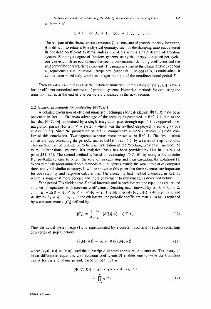
~ , < 0 . o r l A , [ < I, f o r s = 1 .2 . . . . . n.

The real part of the characteristic exponent, i;, is a measure of growth or decay; however, it is difficult to relate it to a physical quantity, such as the damping ratio encountered in constant coefficient systems, unless one deals with a single degree of freedom system. For single degree of freedom systems, using the energy dissipated per cycle. one can establish an equivalence between a conventional damping coefficient and the real part of the characteristic exponent. The imaginary part of the characteristic exponent co, represents a nondimensional frequency. Since t a n - t in eqn (10). is multivalued it can be determined only within an integer multiple of the nondimensional period T.

From this discussion it is clear that efficient numerical computation of [Op(T, 0)] is basis for the efficient numerical treatment of periodic systems. Numerical methods for evaluating the transition matrix at the end of one period are discussed in the next section.

2.2 Numerical methods for evaluating [~(T, 0)] A detailed discussion of efficient numerical techniques for calculating [~(T. 0)] have been

presented in Ref. 1. The main advantage of the techniques presented in Ref. 1 is due to the fact that [OO(T, 0)] is obtained by a single integration pass through eqns (1), as opposed to n- integration passes (for a n × n system) which was the method employed in some previous studies[20.22J. Since the publication of Ref. 1, comparative numerical studies[33] have con- firmed this conclusion. Two separate schemes were presented in Ref. I. The first method consists of approximating the periodic matrix [A(+)] in eqn (1). by a series of step functions. This method can be considered to be a generalization of the "'rectangular ripple" method[15] to multidimensional systems, lt 's analytical basis has been provided by Hsu in a series of papers[34-36]. The second method is based on evaluating [~(T. 0)] by using a fourth-order Runge-Kutta scheme to obtain the solution in each step and then cascading the solutions[ll. When carefully programmed both methods require approximately the same amount of computer time, and yield similar accuracy. It will be shown in this paper that these schemes are important for both stability and response calculations. Therefore, the first method discussed in Ref. 1. which is somewhat more concise and more convenient to implement, is described below.

Each period T is divided into K equal intervals and in each interval the equations are treated as a set of equations with constant coefficients. Denoting each interval by tb~. k = 0, 1, 2, . . . . K, with 0 = Oo < tO, < "'" < OK = T. The kth interval (Ok-,, Ok) is denoted by Tk and its size by Ak = O~ -- O~-,. In the kth interval the periodic coefficient matrix [A(O)] is replaced by a constant matrix [C~] defined by

[Ck] = ~ [A(~)] d~, ~ ~ %. (12)

Thus the actual system, eqn (1), is approximated by a constant coefficient system consisting of a series of step functions

{.~'a(+; K)} = [C(O, K)]{ya(0, K)}, (13)

where tO'a(0, K)} = {y(0)}, and the subscript A denotes approximate quantities. The theory of linear differential equations with constant coefficients[3] enables one to write the transition matrix for the end of one period, based on eqn (13) as

[OPA(T. K)] = e -x~tc'l e -x'-'w' ,I ... e-X,lc,J

K

= FI e<lC'l. k = l

(14)

C¢*~WA 1 2 , 1¢~-J

130 PERETZ P. FRIEDMANN

With regard to the product sign, it is understood that the order of positioning of the factors is material and the kth factor is to be placed in front of the {k - l)th factor. It should be noted that the approximate expression for [O(T, 0)] given by eqn (14) represents the first level of approximation in this method. It can be shown[36] that when K ~ ~c [qbA(T, K)]---, [qb(T, 0)1.

The efficient numerical evaluation of [Oa(T, K)] is accomplished by using the definition of the matrix exponential for each term in the product given by eqn (14); thus

r.

e.~,lc, i = 11] + Y, ('XffCJ)i ,=, j!

15)

For sufficiently small time intervals A i ---* 0 and the series represented by eqn (15) converges rapidly; thus the series can be truncated and represented by a finite number of terms.

~ (&[c,]), ea,lc, I ~_ [11 + j! '

j = l (16)

where the error is given by

y~ (~,[c,])J j=g+, j!

(16a)

The final approximation for the transition matrix at the end of one period is obtained by combining eqns (14) and (16),

[qbaA(T, 0)] = f i ([1] + ~ (A*[C~])'t. i=, j=, J! /

(17)

Equation (16a) represents the error in approximating each matrix exponential of the product given by eqn (14); thus eqn (17) represents a second level of approximation inherent in this method and the double subscript in [~aa(T, 0)] emphasizes this aspect of the method. General asymptotic error estimates for this approximation were obtained in Ref. 36 where it was shown that the error is of order O(A;~) for J -> 2. It should be noted however that these error estimates were not sharp and by increasing the number of terms used in approximating the matrix exponential the accuracy of the method is improved.

Numerical experiments performed in Ref. 1 have shown that the approximation of [qb(T, 0)] with J = 4, based on eqn (17), is comparable to a fourth-order Runge-Kutta method in terms of accuracy and computer times. Furthermore, it is evident that eqn (16) represents an approximation of the matrix exponential by a truncated Taylor series, which represents just one of the many available methods for computing the exponential of a matrix[37,38].

An alternative procedure for evaluating [O(T, 0)] using a fourth-order Runge-Kutta method has been presented in Ref. 1. In a similar manner the transition matrix can be evaluated using a variety of numerical integration procedures which can be implemented in a similar single pass manner[39], which has been emphasized in this section.

3. GENERAL MATHEMATICAL FORM OF PERIODIC SYSTEMS FOR HELICOPTER ROTOR DYNAMICS AND AEROELASTICITY

The general mathematical form of the equations of motion representing the aeroelastic stability and response problem of a helicopter rotor in forward flight have been presented in Ref. 2. These are coupled ordinary differential equations with periodic coefficients. The mathematical structure of these general equations can be presented in the following symbolic form:

[M]{(/} + [C(+)]{0} + [K(+)I {q} = {FNL(dJ. q. q)}. (18)


where it is understood that the matrix [C(O)] contains aerodynamic, inertial and viscous damping contributions, while the matrix [K(0)] contains aerodynamic, inertia as well as structural contributions. In this formulation all nonlinear effects and the excitation are combined in the general vector {FNL(+, q, el)]. The nonlinear terms in those equations can be geometrical nonlinearities, due to moderate blade deflections or aerodynamic nonlinearities due to dynamic stall[2l. The mathematical methods discussed in this paper are particularly useful when dealing with geo- metrically nonlinear terms, which are weak nonlinearities. When dynamic inflow is considered. the dynamic inflow equations have to be appended to eqns (18) and solved jointly[2,40].

The mathematical and numerical treatment of eqns (18) is facilitated by rewriting them in first order state variable form; thus

{y,(+)} = {//(~)}, {y2(t~)} = {q(+)} (19)

and eqn (19) can be rewritten as

{)'} = {Qst.(+. )', y)} = {Z(~)} + [L(~)] {y} + {N,(+, y)} + {N..(+, y,~')}, (20)

where

and

I - [M]- ' [C(O) ] - [ M I - ' [ K ( + ) ]

[L(+)] = [t] 0 (21)

with

(

{Z($)} + {Ni0b, Y)} + {N,(O, y, ~')} = ~ - [ M I - ' F~L(O, y,, y:)~ [ {o} j (22)

{Y(0)} = ly:(,) j

It should be noted this transformation doubles the size of the system represented by eqns (20) when compared to eqn (19). Since the system is periodic with a period of 2~.

{Z(,)} = {Q(t~ + 2'rr)}, (23)

[L(0)I = [L(d~ + 2~)1, (24)

{N,(~, y)} = {N,(d~ + 2"rr, y)} (24a)

and

{N2(*, Y, $9} = {Nx(dJ + 2w, y, $9}. (24b)

The vector {Z(0)} represents a known excitation, the matrix [L(~)] contains the periodic coefficients of the linear system, and the vectors {N~(~, y)} and {N,(tb, y, y)} represent the nonlinear terms in the equations, and {Y(0)} is the state of the system.

The numerical techniques for obtaining the response of both linear and nonlinear periodic systems, discussed in the following sections will be based on the mathematical form of the equations represented by eqn (20).

4. RESPONSE OF LINEAR PERIODIC SYSTEMS

Consider first the linear part of the general aeroelastic response problem represented by

13S

eqn (20). which can be written as

P[ REFZ P. FR[I 1)\1 \ ~ , \

{.+(,b)} = {Z(+)} * I L l ~ b l l ] v { , I J ) } . ~25~

Both the system of equations and the excitation for the rotary-~ving aeroelastic response problems are periodic, as indicated by eqns (23) and (24).

The associated homogeneous system is given by

{i'~,(¢,)1. = ILOJ,)l{.v,,(+)l. (26)

which is identical to eqn (1). Urabe[41] has shown that for characteristic muhipliers of the corresponding homogeneous system, eqn (26). which are different from one. i.e. a stable or unstable homogeneous system according to Floquet theory, one has one and onh' one periodic solution of eqn (25) given by

{y(+)} : [qb(¢,)] { ; ; [dO(s)l-~{Z(s)} ds + (Ill - [~(2w)l) '

* ,@,2w)l f f [q)(s)]- '{Zts)} ds} . 127)

The general solution for any inhomogeneous equation such as eqn {25) whether periodic or not can be mathematically written as[42]

j 'd~

{y(+)} = [~(+)l{y(0)} + Iqt, t+)l [@ts)l '{Z(s)} ds. I28)

where in eqns (27) and (28) [q~(0)l is the transition matrix defined by

[do(O)l = [LI+)I[~I~b)I

and [dP(0)l = [/l. Note that the condition for the existence of a unique periodic solution of eqn (25) is that

the determinant of ([I] - [~(2rr)]) be nonzero. This is satisfied if all the multipliers of eqn (26), the A/s, are different from unity, which is equivalent to the condition that the real parts of all characteristic exponents be nonzero, i.e. 4, # O. From Floquet theory, if all the ~,'s < O, the homogeneous system is asymptotically stable: if any one 4, > 0. the homogeneous system becomes asymptotically unstable. In the former case eqn (27) is the steady state solution of the linear system eqn (25). When any one to, > O, the mathematical expression for {.v(O)}. eqn (27), is still valid, however the periodic solution of eqn (25) is of no practical physical signif- icance; Hsu and Cheng[43] have made some interesting comments in this respect.

Comparing eqns (27) and (28) it is obvious that eqn (27) corresponds to the general solution of any inhomogeneous system, eqn (28) with the initial condition given by

{y(0)} = ([ll - [~(2ml)-'[qb(2~v)] [dp(s)l-'{Zts)} ds.

Equation (29) can be simplified by rewriting it in a more convenient manner:

129)

{y(0)} = ([/1 - [~(2~)1) ' [~(2w)ll~(.s){ '{ZCs)} dx. 130~


Using the semigroup property of the transition matrix. Ref. 10. p. 29 (sometimes denoted the extension property) which establishes a functional equation for the transition matrix

[@(~. +o)l = [@(+. +01[@(~,, tOo)l.

one can express

[O(2w. 0)1 = [~(2,-r, s)l[~(s, 0)1. (31)

Postmultiplying each side of eqn (31) by [q~(s, 0)1- ~ yields

[~(2w)l[qb(s, 0)1-' = [dO(2~, s)]. (32)

Substitution of eqn (32) into eqn (30) yields

fo ~ {y(0)} = ([1] - [~b(2,rr)])-' [qb(2rr, s)l{Z(s)} ds. (33)

Equation (33) is more convenient for the calculation of the initial condition {y(0)}, eqn (29), since it does not require the inversion of [qb(s)l. A very similar solution technique is also described in Ref. 31. The approximation to the transition matrix given, eqn (17) can be also employed to calculate the value of [~(2~, s)] needed in order to evaluate numerically the initial condition {y(0)}, given by eqn (33). The value of the integral in eqn (33) can be evaluated using any conventional integration procedure such as Simpson's rule. This procedure for gen- erating the initial condition is described in detail and used in Ref. 44.

Taking the initial condition, eqn (33). the linear system represented by eqn (25) is integrated numerically using a fourth-order, Runge-Kutta scheme, with Gill coefficients[ 1 ]. The integration is performed with a constant step size which is identical to the step size used in evaluating the transition matrix at the end of one period [qb(T, 0)l. This means that the use of eqn (27) is actually, completely, bypassed. Convergence of the method is checked by comparing the dis- placement quantities obtained for the response at the end of the first, or second revolution with the initial conditions, i.e. compare

{y(O)} with {y(2~)}, or {y(4w)}, or {y(6w)}.

Depending on the numerical accuracy of the calculations excellent converged solutions can be obtained with one to three revolutions.

5. RESPONSE OF NONLINEAR PERIODIC SYSTEMS

The solution of the complete nonlinear system represented by eqn (20) is considered next. When the nonlinearities are relatively mild a number of approaches are available and have been used successfully to obtain the nonlinear response of rotor blades in forward flight. Three approaches which have been used are (a) quasilinearization[27,28], (b) periodic shooting[29,30] and (c) harmonic balancing[31]. Quasilinearization and periodic shooting, depending on the implementation and application, can be equally effective. Harmonic balancing is less convenient to use[31] although some recent developments and extensions of the method[45] indicate that this method can be also quite effective. An alternative to these methods is a numerical perturbation method described in Ref. 3 I, which appears to work only for mildly nonlinear systems.

The approaches described in this paper are quasilinearization and periodic shooting: other methods will be mentioned briefly. Quasilinearization is essentially a generalized Newton- Raphson type method possessing second-order convergence[461. The quasilinearization scheme described here is based on an iterative application of the method for obtaining the linear response of periodic systems described in the previous section[30]. Introducing an iteration index k for obtaining the nonlinear periodic response of eqn (20) one can perform a first-order Taylor series

1 4 i ) PERETZ P. FRIEDMANN

expansion about the #th iteration,

r Q, l' , ,_ {.+}~.t = {Qyc}' + L- -~-y J ({yt ' - {y}*) + L a~, j (b}'-' - {~'}')

(34)

which enables one to write a linear equation in the form

{5,} *+, = [Ap{y} ~*' + {f}~. (35)

Equation (35) is obtained as follows. Express QNt_ as given by eqn (20) and substitute it into eqn (34). Then [A] and {f} in eqn (36) can be identified as

L all / L a y j L - ~ y J / (36)

and

( P :l'l {f}' = [11 - k O}'J /

+ {N_,(0, y, y)}~

- - k

-'i{Z(O)}[" + {N.(+, y.)}~

_ O N , ~

(37)

To initiate the iterative procedure, the nonlinear terms {Nff0, y)} and {N_,(O, y, .';9} are dropped from {QNt.} and the resulting linear system, eqn (25), is solved for a periodic solution which provides an initial guess; thus {y}0 = {Yc}, where {YL} is the periodic response of eqn (25) and is obtained by the method described in the previous section. This method is also used to solve eqn (35) for k = 1, 2 . . . . Thus quasilinearization is a sequence of linear iterates based upon eqns (35), (36) and (37). For the cases which have been considered[27,28] the derivatives of Na and N_, were evaluated explicitly. The iterations are terminated when the L,- norm

II({y} k÷' - {y}*)ll; < e, (38)

for all O, where e is a prescribed small parameter. Thus k = ! corresponds to the linearized response and k = 2 corresponds to the first approximation of the nonlinear periodic response.

The nonlinear periodic shooting method[29,30] is based on integrating eqn (20) with an estimated initial condition {y(0)} over one period. The integrated solution {y(T)} is not periodic, and can be regarded as a first estimate of the periodic solution {Ye}" The initial conditions can be modified so as to make {y(T)} periodic, applying this procedure in an iterative manner eventually leads to a solution.

The mathematical basis of this method consists of using as initial condition the relation[30,31 ]

{y(O)} = ([11 - [qb(2~r)])-'{ye(2"rr)}, (39)

where {yE(2w)} is the numerical response of the linear system, eqn (25), at 0 = T (or 27) for zero initial conditions. This initial condition, eqn (39) is identical to eqn (33), and thus it guarantees a periodic response for the linear system. Since the system represented by eqn (20) is nonlinear, numerical integration over one period will not yield a periodic solution. Theretbre, the method of periodic shooting is based on successive iteration on the initial values in order to satisfy the periodic boundary condition. In each stage of the iteration the full nonlinear equations are solved, while the error in the periodic boundary condition is driven to zero. The


periodic shooting method described in Ref. 30 is a two point periodic shooting method for which the algorithm has the following structure:

(1) Initial guess for the state vector at the beginning of the period is based on eqn (39). (2) The nonlinear system is integrated over one period using a suitable numerical integration

method. (3) The sensitivity matrix for the state vector at the end of period is expressed in terms

of perturbations in the values of state vector at the beginning of the period, denoting the sensitivity matrix by [S]i, for the ith iteration

= [ O{ys}] (40) (Sl, kO{yo}J, '

where {Ys}~ is the final state vector for the ith iteration and {Y0} is the initial state vector for the ith iteration.

(4) Using the sensitivity information given by eqn (40) a revised vector of initial values is calculated, so that the periodic boundary conditions are satisfied. The revised vector of initial conditions for the (i + l)th iteration is given by

{Yo};+, = {Y0}, + ([/l - [S],)- ' ({Yl},- {Yo},). (41)

(5) The nonlinear equations are integrated again over one period using the revised initial condition given by eqn (41).

(6) The periodicity condition is checked within a desired accuracy

I{Yf},*, - {yo}i+,l < ~- (42)

If eqn (42) is satisfied the iteration is stopped. If eqn (42) is violated, one returns to step (3), and the procedure is repeated until convergence is obtained.

A somewhat similar procedure called numerical perturbation is also described in Ref. 31. Comparative numerical studies between quasilinearization and periodic shooting for rotary-wing aeroelastic problems were conducted in Ref. 44. It was shown that the methods are equally efficient in terms of computer times. However, it should be noted that the two point periodic shooting described in Ref. 44 used a somewhat more efficient method for calculating the sensitivity matrix [S]i, eqn (40), than the finite difference method used in previous studies[30]. A careful examination of eqn (40) shows that infinitesimal changes in the initial values {Y0}~ cause infinitesimal changes in the baseline nonlinear solution {y}, Due to the infinitesimal nature of these changes, they are governed by the linearized perturbed system about the baseline solution {y}~; furthermore, it can be shown that this perturbed system is homogeneous. Therefore, the sensitivity matrix for the final values, with respect to the initial values, is simply the transition matrix of the linear perturbed system[44]. This transition matrix can be evaluated using eqn (17), and thus the need to use a finite difference scheme for the calculation of the sensitivity matrix is bypassed. Furthermore, multiple periodic shooting methods were also considered and tested[44]; it was concluded the success of shooting as well as quasilinearization methods can depend to some extent on the type of problems to which the methods are applied.

6. AEROELASTIC STABILITY OF ROTOR BLADES IN FORWARD FLIGHT USING THE LINEARIZED SYSTEM

When the system is mildly nonlinear, which is the case when geometric nonlinearities due to moderate blade deflections are incorporated in the blade equations of motion, a considerable number of studies[2,44,48-501 have indicated that a reliable measure of system stability can be obtained from the linearized system. Denoting by {Fl(~b) } the time-dependent periodic equilibrium of the blade, obtained from solving eqn (20) using the method described in Section 5,

14.2 PEREFZ P. FRIIDM \\ '~

the perturbed state about this equilibrium position can be ~ritten as

{q(o)} = {0(o)} ÷ {_xq +IL

Substituting this relation into eqn (18) and assuming that squares of the perturbation quantities, namely Aq,(tL,) &qi(O). are small and negligible, one obtains a [inearized homogeneous system which can be symbolically written in a first-order state variable form. as

{_k~} = [LOb. ?l,l~))] {3y}. (43)

where

{,_x:,} = ±q

and [L(O,.v(0))] is a coefficient matrix, similar to eqn (21). which depends on both the nondimensional time 0, and the nonlinear periodic equilibrium state of the blade {.~(0)}. The matrix [L(+,~(+))] is also a periodic matrix: hence the equilibrium of the system, eqn 143), can be obtained from Floquet theory by evaluating the characteristic exponents as described in Section 2. This approach has been used successfully in many recent studies dealing x~ith forward flight[2,44.48-50].

7. NUMERICAL ASPECTS OF THE METHODS DISCUSSED AND SOME ILLUSTRATIVE RESULTS

The purpose of this section is to describe various examples where the methods described in this paper were applied to rotor dynamics, and helicopter rotor blade aeroelastic stability and response calculations. The primary intent is to present information on the numerical aspects. convergence and efficiency of the methods instead of reproducing numerical results which were presented in the various references cited.

First the methods for evaluation of the transition matrix at the end of one period [O(T, 0)], described in Section 2.2, are discussed. These methods have been used first in Refs. 1, 23 and 24 and subsequently in Refs. 25-28, 44. Transition matrices of size ( 12 × 12) have been treated without any numerical difficulties. For larger systems double precision in thc calculation of the transition matrix on IBM machines is usually required. The stepsize used varies between 60 < K < 120 per revolution. For the same step size the computations based on eqn (17) and the fourth-order Runge-Kutta scheme are equally effective[l]. Considerable information on numerical experimentation involving accuracy, convergence and computing times can be found in Ref. 1. Furthermore, it should be noted that the method has been also used in conjunction with a finite element method employed to descretize the spatial properties of the aeroelastic equations of motion[47].

The method based on the application of eqn (33) combined with numerical integration to obtain the response of a linear periodic system was developed initially for the linear periodic response problems of horizontal axis wind turbines[25,26], where a somewhat more cumbersome version of eqn (33), namely eqn (29) was used.

Subsequently this method was applied to the linear and nonlinear response problem of helicopter rotor blades in tbrward flight, in presence of quasisteady aerodynamic loads[27.28,47]. and more recently, with the improvement represented b; eqn (33) in Ref. 44. to helicopter rotor blades in forward flight, in presence of unsteady aerodynamic loads. For linear response calculations the stepsize required for the implementation of the method was similar to the number of steps needed for the calculation of the transition matrix [4)IT, 0)]. thu_. 60 < K < 120, per revolution.

The quasilinearization method described in Section 5. is based on an iterative application of the linear response calculation described in Section 4. For application to nonlinear periodic system response calculations, using eqn (35). the number or'steps which provided good numerical

Numerical methods for determining the stability and respt)nse of periodic systems

0.12

gl (~), g2 (~)'~ " 0"t~ O K'O

K '2

0.02

0.00

0 30

-~ 0.10 1

~" 0.06

5 0.06

Z ~ 0 . 0 4

90 180 270 360

PSI (DEGREES)

143

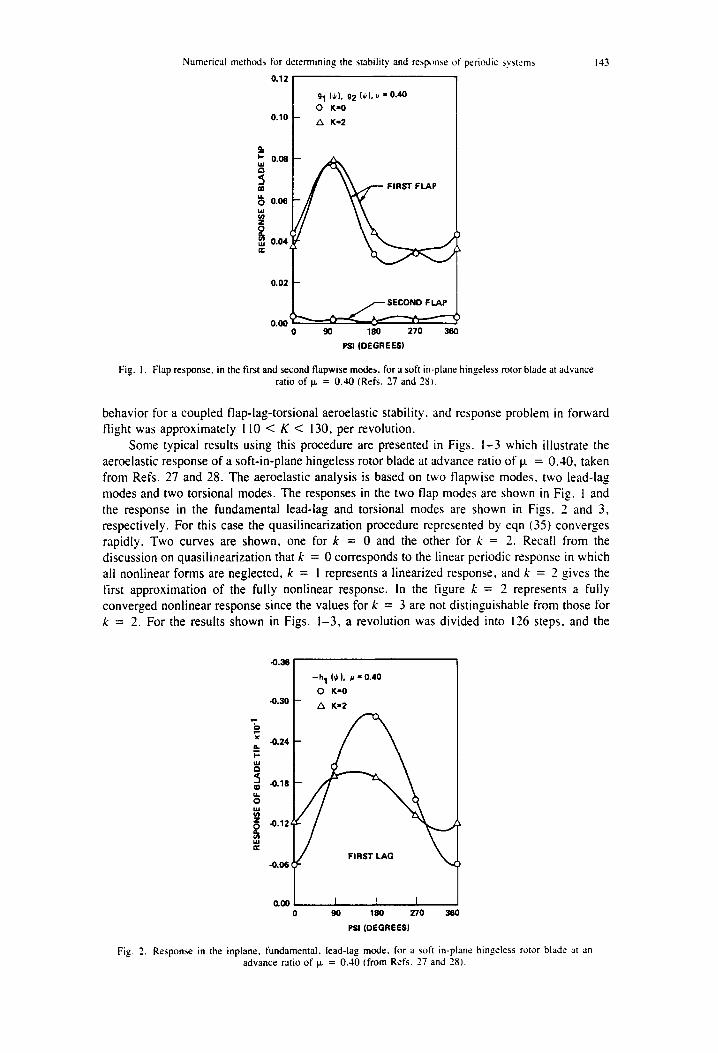
Fig. 1. Flap response, in the first and second flapwise modes, for a soft in-plane hingeless rotor blade at advance ratio of ~ = 0.40 (Refs. 27 and 281.

behavior for a coupled flap-lag-torsional aeroelastic stability, and response problem in forward flight was approximately 110 < K < 130, per revolution.

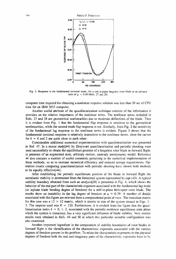
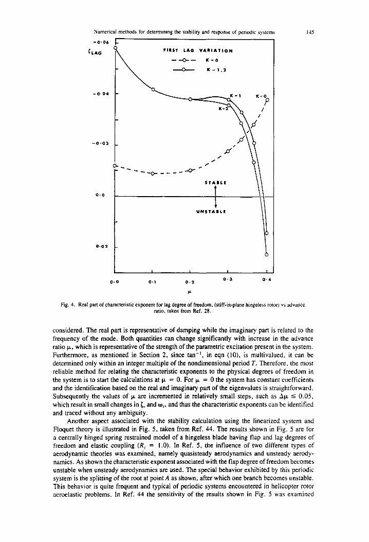
Some typical results using this procedure are presented in Figs. I - 3 which illustrate the aeroelastic response of a soft-in-plane hingeless rotor blade at advance ratio of tx = 0.40, taken from Refs. 27 and 28. The aeroelastic analysis is based on two flapwise modes, two lead-lag modes and two torsional modes. The responses in the two flap modes are shown in Fig. 1 and the response in the fundamental lead-lag and torsional modes are shown in Figs. 2 and 3, respectively. For this case the quasilinearization procedure represented by eqn (35) converges rapidly. Two curves are shown, one for k = 0 and the other for k = 2. Recall from the discussion on quasilioearization that k = 0 corresponds to the linear periodic response in which all nonlinear forms are neglected, k = ! represents a linearized response, and k = 2 gives the first approximation of the fully nonlinear response. In the figure k = 2 represents a fully converged nonlinear response since the values for k = 3 are not distinguishable from those for k = 2. For the results shown in Figs. 1-3, a revolution was divided into 126 steps, and the

- h 1 (~), ~ - 0 . 4 0

O K-0

K-2

2 x -0.24

-~ -0.18

~ 41.12,

w

°0.06

0.0o I ! I 0 90 180 270 360

PSI (DEGREES) Fig. 2. Response in the inplane, fundamental, lead-lag mode. for a soft in-plane hingeless rotor blade at an

advance ratio of Ix = 0.40 (from Refs. 27 and 28).

144

i 0.01

-0.01

-0.03

-0.05

-0.07

PERETZ P. FRIEDMCNN

0 0E ] fl (" 1" " = 0.40

O K:0

0.03

I I t 90 180 270 360

PSI (DEGREES)

Fig. 3. Response in the fundamental torsional mode, /or a soft in-plane hingeless rotor blade at an advance ratio of/,t = 0.40 (Refs. 27 and 28).

computer time required for obtaining a nonlinear response solution was less than 30 sec of CPU time for an IBM 3033 computer.

Another useful attribute of the quasilinearization technique consists of the information it provides on the relative importance of the nonlinear terms. The nonlinear terms included in Refs. 27 and 28 are geometrical nonlinearities due to moderate deflections of the blade. Thus it is evident from Fig. 1 that the fundamental flap response is sensitive to the geometrical nonlinearities, while the second mode flap response is not. Similarly, from Fig. 2 the sensitivity of the fundamental lag response to the nonlinear terms is evident. Figure 3 shows that the fundamental torsional response is relatively insensitive to the nonlinear terms, since the curves for k = 0 and 2 are quite close to each other.

Considerable additional numerical experimentation with quasilinearization was presented in Ref. 47. In a recent study[44] by Dinyavari quasilinearization and periodic shooting were used successfully to obtain the equilibrium position of a hingeless rotor blade in forward flight, in presence of an augmented state, arbitrary motion, unsteady aerodynamic model. Reference 44 also contains a number of useful comments pertaining to the numerical implementation of these methods, so as to increase numerical efficiency and reduced storage requirements. Op- eration counts comparing quasilinearization with periodic shooting have shown both methods to be equally effective[44].

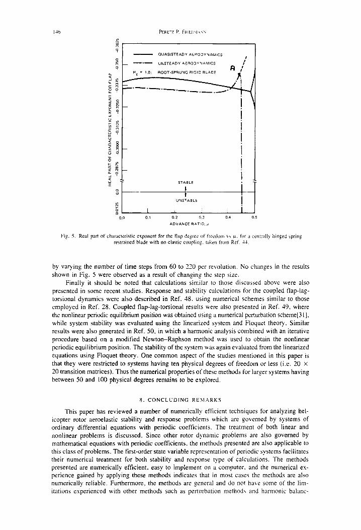
After establishing the periodic equilibrium position of the blade in forward flight the aeroelastic stability is determined from the linearized system represented by eqn (43). A typical stability boundary obtained from such an analysis[28] is presented in Fig. 4, which shows the behavior of the real part of the characteristic exponent associated with the fundamental lag mode (or inplane blade bending degree of freedom) for a stiff-in-plane helicopter rotor blade. The results show an instability in the lag degree of freedom at p. ~ 0.39. A number of details associated with this figure are relevant from a computational point of view. The transition matrix for this case was a 12 × 12 matrix, which is similar in size of the system treated in Figs. 1- 3. The stepsize used was K = 120. Furthermore, it is evident from the figure that the quasilinearization index k = 0, 1, 2, associated with the periodic nonlinear equilibrium state about which the system is linearized, has a very significant influence of blade stability. Very similar results were obtained in Refs. 49 and 50 in which this particular unstable configuration was also examined.

Another important ingredient in the computation of stability boundaries of rotor blades in forward flight is the identification of the characteristic exponents associated with the various degrees of freedom present in the problem. To relate the characteristic exponents to the physical degrees of freedom both the real and imaginary parts of the characteristic exponents have to be


- - 0 " 0 6

~LAG

--0"04

- 0 " 0 2

0 . 0

0 .02

I- FIRST LAG V A R I A T I O N

- - "-(~- - - K : 0

O K ~ 1 , 2

K - I K = ~

/

J

H f

STABLE

I UNSTABLE

0 .0

I I

0.1 0 . 2 0 . 3 0"4

Fig. 4. Real part of characteristic exponent for lag degree of freedom, (stiff-in-plane hingeless rotor) vs advance ratio, taken from Ref. 28.

considered. The real part is representative of damping while the imaginary part is related to the frequency of the mode. Both quantities can change significantly with increase in the advance ratio ~, which is representative of the strength of the parametric excitation present in the system. Furthermore, as mentioned in Section 2, since tan -1, in eqn (10), is multivalued, it can be determined only within an integer multiple of the nondimensional period T. Therefore, the most reliable method for relating the characteristic exponents to the physical degrees of freedom in the system is to start the calculations at Ix = 0. For i~ = 0 the system has constant coefficients and the identification based on the real and imaginary part of the eigenvalues is straightforward. Subsequently the values of ix are incremented in relatively small steps, such as Aix -- 0.05, which result in small changes in g~ and cos, and thus the characteristic exponents can be identified and traced without any ambiguity.

Another aspect associated with the stability calculation using the linearized system and Floquet theory is illustrated in Fig. 5, taken from Ref. 44. The results shown in Fig. 5 are for a centrally hinged spring restrained model of a hingeless blade having flap and lag degrees of freedom and elastic coupling (R, = 1.0). In Ref. 5, the influence of two different types of aerodynamic theories was examined, namely quasisteady aerodynamics and unsteady aerodynamics. As shown the characteristic exponent associated with the flap degree of freedom becomes unstable when unsteady aerodynamics are used. The special behavior exhibited by this periodic system is the splitting of the root at point A as shown, after which one branch becomes unstable. This behavior is quite frequent and typical of periodic systems encountered in helicopter rotor aeroelastic problems. In Ref. 44 the sensitivity of the results shown in Fig. 5 was examined

146

?

c5 u. J

e,i

Lu

cJ

F-

< - r .

'il 0.0

PERETZ P. FRIED\I ".'-,",

Q U A S I S T E A D Y A E R O D Y N A M I C S

__ ~ ° ~ U N S T E A D Y A E R O D Y N A M I C S #

A / R c " 1.0: ROOT-SPRUNG RIGID BLADE I ( l

2 - . . - - -

I I I i I

STABLE

UNSTABLE I

I I I I 0.1 0.2 03 0.4

ADVANCE RAT$O, ,~

0.5

Fig. 5. Real part of characteristic exponent for the flap degree or freedom vs ¢t. for a centrally hinged spring restrained blade with no elastic coupling, taken from Ref. 44.

by varying the number of time steps from 60 to 220 per revolution. No changes in the results shown in Fig. 5 were observed as a result of changing the step size.

Finally it should be noted that calculations similar to those discussed above were also presented in some recent studies. Response and stability calculations for the coupled flap-lag- torsional dynamics were also described in Ref, 48, using numerical schemes similar to those employed in Ref. 28. Coupled flap-lag-torsional results were also presented in Ref. 49, where the nonlinear periodic equilibrium position was obtained using a numerical perturbation scheme[31 ], while system stability was evaluated using the linearized system and Floquet theory. Similar results were also generated in Ref. 50, in which a harmonic analysis combined with an iterative procedure based on a modified Newton-Raphson method was used to obtain the nonlinear periodic equilibrium position. The stability of the system was again evaluated from the linearized equations using Floquet theory. One common aspect of the studies mentioned in this paper is that they were restricted to systems having ten physical degrees of freedom or less (i.e. 20 x 20 transition matrices). Thus the numerical properties of these methods for larger systems having between 50 and 100 physical degrees remains to be explored.

8. CONCLUDING REMARKS

This paper has reviewed a number of numerically efficient techniques for analyzing helicopter rotor aeroelastic stability and response problems which are governed by systems of ordinary differential equations with periodic coefficients. The treatment of both linear and nonlinear problems is discussed. Since other rotor dynamic problems are also governed by mathematical equations with periodic coefficients, the methods presented are also applicable to this class of problems. The first-order state variable representation of periodic systems facilitates their numerical treatment for both stability and response type of calculations. The methods presented are numerically efficient, easy to implement on a computer, and the numerical ex- perience gained by applying these methods indicates that in most cases the methods are also numerically reliable. Furthermore, the methods are general and do not have some of the lim- itations experienced with other methods such as perturbation methods and harmonic balanc-


ing[31]. On the other hand, it should be noted that additional research is needed to establish the reliability of such methods for larger systems which would be governed by state vectors containing 50 to 100 state variables.

Acknowledgement--The constructive comments made by Dr. Ron Dinyavari are hereby gratefully acknowledged.

REFERENCES

I. E Friedmann. C. E. Hammond and T, Woo. Efficient Numerical Treatment of Periodic Systems with Application to Stability Problem. Ira. J. Numer. Methods Engng II, 1117-1136 (1977)

2. E P. Friedmann, Formulation and Solution of Rotary-Wing Aeroelastic Stability and Response Problems. Vertica 7, 101-141 (1983).

3. E. A. Coddington and N. Levinson. Theory of Ordinary Differential Equations. McGraw-Hill. New York (1955). 4. L. A. Pipes and L. R. Harvill, Applied Mathematics for Engineers and Physicists, 3rd Edn. McGrav.-Hill, New

York (1970). 5. N. P. Erugin, Linear Systems of Ordinary Differential Equations with Periodic and Quasi-Periodic Coefficients.

Academic, New York (1966). 6. V. A, Yakubovitch and X, Starzhinskii, Linear Differential Equations with Periodic Coefficients. Vols. I and II.

Halsted, Wiley, New York, (Israel Program for Scientific Translations) (1975). 7. W. Magnus and S. Winkler. Hill's Eq,,ation. Wiley, New York (1966). 8. E M. Arscott, Periodic Differential Equations. Pergamon. Oxford (1964). 9, H. D'Angelo, Linear Time-Varying Systems: Analysis and Synthesis. Allyn and Bacon, Boston (1970).

10. R. W. Brocket. Finite Dimensional Linear Systems. Wiley. New York (1970). I I. J. A. Richards, Ana(vsis of Periodically Time-Va~'ing Systems, Springer-Verlag. New York (1983). 12. V. V. Bolotin. Dynamic Stabili~.' of Elastic Systems. Holden-Day, San Francisco (1964). 13. A. H. Nayfeh and D. T. Mook, Nonlinear Oscillations. Wiley, New York (1979). 14. W. Johnson, Helicopter Theory. Princeton Univ. Press (1980). 15. G. Horvay and S. W. Yuan, Stability of Rotor Blade Flapping Motion when the Hinges are Tilted, Generalization

of the "'Rectangular Ripple" Method of Solution. J. Aeronaut. Sci. 14, 583-593 (1947). 16. G. J. Sissingh, Dynamics of Rotor Operating at High Advance Ratios. J. Am, Helicopter Soc. 13.56-63 (1968). 17. G. J. Sissingh and W. A. Kuczynski, Investigation on the Effects of Blade Torsion on the Dynamics of the Flapping

Motion at High Tip Speed Ratios. J. Am. Helicopter Soc. 15.2-9 (1970). 18. O. J. Lowis, The Stability of Rotor Blade Flapping Motion at High Tip Speed Ratios. Aeronautical Research

Council, London. England, R&M 3544 (January, 1963). 19. P. Crimi, A Method for Analyzing the Aeroelastic Stability of a Helicopter Rotor in Forward Flight. NASA CR-

1332 (August 1969). 20. W. E. Hall, Application of Floquet Theory to the Analysis of Rotary Wing VTOL Stability. SUDDAR 400. Feb.

1970. Stanford University Center of Systems Research, Palo Alto, CA. 21. M. A. Gockel. Practical Solution of Linear Equations with Periodic Coefficients. J. Am. Helicopter Soc. 17. 2-

10 (1972). 22. D. A. Peters and K. H. Hohenemser, Application of the Floquet Transition Matrix to Problems of Lifting Rotor

Stability. J. Am. Helicopter Soc. 16, 25-33 (1971). 23. C, E. Hammond, An Application of Floquet Theory to Prediction of Mechanical Instability. J, Am. Helicopter

Soc. 19, 14-23 (1974). 24. P. Friedmann and L. J. Silverthorn, Aeroelastic Stability of Periodic Systems with Application of Rotor Blade

Flutter. AIAA J. 12, 1559-1565 (1974). 25. S. B. R. Kottapalli. P. P. Friedmann and A. Rosen, Aeroelastic Stability and Response of Horizontal Axis Wind

Turbine Blades. Paper C4, Proceedings of Second International Symposium on Wind Energy Systems. BHRA Fluid Engineering, Cranfield. October 1978, Vol. I, pp. C4-49-C4-66.

26. S. B. R. Kottapalli, P. P. Friedmann and A. Rosen, Aeroelastic Stability and Response of Horizontal Axis Wind Turbine Blades. AIAA J. 17. 1381-1389 (1979).

27. P. P. Friedmann and S. B. R. Kottapalli, Rotor Blade Aeroelastic Stability and Response in Forward Flight. Paper No. 14, Proceedings of the 6th European Rotorcraft and Powered Lift Aircraft Forum, Bristol. England, September 1980.

28. P. P. Friedmann and S. B. R. Kottapalli, Coupled Flap-Lag-Torsional Dynamics of Hingeless Rotor Blades in Forward Flight. J. Am. Helicopter Soc. 27, 28-36 (1982).

29. A. P. izadpanah, Helicopter Trim and Air Loads by Periodic Shooting with Newton-Raphson Interation. M.S. thesis. Sever Institute of Technology. Washington University, St. Louis. December 1979.

30. D. A. Peters and A. P. Izadpanah. Helicopter Trim by Periodic Shooting with Newton-Raphson Iteration. Pro- ceedings 37th Annual Forum of the American Helicopter Society, New Orleans. 1981. pp. 217-226.

31. J. Dugundji and J. H. Wendell, Some Analysis Methods for Rotating System. with Periodic Coefficients. AIAA J. 21. 890-897 (1983).

32. B. Noble. Applied Linear Algebra. Prentice Hall. Englewood Cliffs. NJ (1969). 33. G. H. Gaonkar. D. S. Prasad and D. Sastry. On Computing Floquet Transition Matrices for Rotorcraft. J. Am.

Helicopter Soc. 26. 56-61 ( 198 I). 34. C. S. Hsu, Impulsive Parametric Excitation: Theory. J. Appl. Mech. 39, 551-558 (1972). 35. C. S. Hsu and W. H. Cheng, Applications of the Theory of Impulsive Parametric Excitation and New Treatments

of General Parametric Excitation Problems. J. Appl. Mech. 40, 78-86 (1973). 36. C. S. Hsu. On Approximating a General Linear Periodic System. J. Math. Anal. Appl. 45, 234-251 (1974). 37. C. Moler and C. Van Loan. Nineteen Dubious Ways to Compute the Exponential of a Matrix. SL4M Rev. 20.

801-836 (1978). 38. G. J. Bierman. Power Series Evaluation of Transition and Covariance Matrices. IEEE Trans. Atttomatic Control

228-232 (April 1972).

14S PERETZ P. FRIED'~AN'q

39. C. Von Kerczek, Calculation of Transition Matrices. A[AA J. 13. 1401-1403 (1975). 40. D. A. Peters and G. H. Gaonkar. Theoretical Flap-Lag Damping with Various Dynamic Intlow Models. J. Am

Helic~)pter Soc. 25, 29-36 (1980). 41. M. Urabe, Galerkin's Procedure for Nonlinear Periodic Systems, Arch. Rational Mech. Anal. 211. 120-152 11965 I. 42. H. K. Wilson, Ordinary Differential Equations, p. 117. Addison-Wesley, Reading, MA i l971k 43. E, S. Hsu and W. H. Cheng. Steady-State Response of a Dynamical System Under Combined Parametric and

Forcing Excitation. J. Appl. Mech. 41. No. 2, pp. 371-378 (1974). 44. M. A. H. Dinyavari. Unsteady Aerodynamics in Time and Frequency Domains for Finite-Time Arbitrary Motion

of Helicopter Rotor Blades in Hover and Forward Flight. Ph.D, dissertation, Mechanical, Aerospace and Nuclear Engineering Department, University of California at Los Angeles. March 1985.

45. S. S. Lau, Y. K. Cheung and S. Y. Wu, A Variable Parameter [ncrementation Method for Dynamic lnstabilit', of Linear and Nonlinear Systems. J. Appl. Mech. 49. 849-853 (1982).

46. S. M. Robets and J. S. Shipman, Two Point Boundary Value Problems: Shooting Methods, pp. 87-109. Elsevier, New York i1972).

47. F, K. Straub and P, P. Friedmann, Application of the Finite Element Method to Rotary-Wing Aeroelasticity. NASA CR-165854 (February 1982).

48. G. R. Nilakantan and G. H. Gaonkar, Feasibility of Simplifying Coupled Flap-Lag-Torsional Models for Rotor Blade Stability in Forward Flight. Paper No. 53. Tenth European Rotorcraft Forum. The Hague, Netherlands, August 28-31, 1984. pp. 53.1-53.31.

49. B. Panda and 1, Chopra, Flap-Lag-Torsion Stability in Forward Flight. Paper No. 16, Proceedings of Second Decennial Specialists Meeting on Rotorcraft Dynamics, Ames Research Center, Moffett Field, Nov. 7-9, 1984.

50. T. S. R. Reddy and W. Warmbrodt. The Influence of Dynamic Inflow and Torsional Flexibility on Rotor Damping in Forward Flight from Symbolically Generated Equations. Paper No. 15. Proceedings of Second Decennial Specialist's Meeting on Rotorcraft Dynamics, Ames Research Center. Moffett Field, Nov. 7-9, 1984.

NUMERICAL METHODS FOR DETERMINING THE … · successfully in helicopter rotor dynamics and...

Documents

Transcript of NUMERICAL METHODS FOR DETERMINING THE … · successfully in helicopter rotor dynamics and...