ACTAUNIVERSITATIS

UPSALIENSISUPPSALA

2017

Digital Comprehensive Summaries of Uppsala Dissertationsfrom the Faculty of Science and Technology 1495

Numerical Methods for DarcyFlow Problems with Rough andUncertain Data

FREDRIK HELLMAN

ISSN 1651-6214ISBN 978-91-554-9872-6urn:nbn:se:uu:diva-318589

Dissertation presented at Uppsala University to be publicly examined in ITC 2446,Lägerhyddsvägen 2, Uppsala, Friday, 19 May 2017 at 10:15 for the degree of Doctor ofPhilosophy. The examination will be conducted in English. Faculty examiner: ProfessorRobert Scheichl (Department of Mathematical Sciences, University of Bath).

AbstractHellman, F. 2017. Numerical Methods for Darcy Flow Problems with Rough andUncertain Data. Digital Comprehensive Summaries of Uppsala Dissertations from theFaculty of Science and Technology 1495. 41 pp. Uppsala: Acta Universitatis Upsaliensis.ISBN 978-91-554-9872-6.

We address two computational challenges for numerical simulations of Darcy flow problems:rough and uncertain data. The rapidly varying and possibly high contrast permeabilitycoefficient for the pressure equation in Darcy flow problems generally leads to irregularsolutions, which in turn make standard solution techniques perform poorly. We study methodsfor numerical homogenization based on localized computations. Regarding the challenge ofuncertain data, we consider the problem of forward propagation of uncertainty through anumerical model. More specifically, we consider methods for estimating the failure probability,or a point estimate of the cumulative distribution function (cdf) of a scalar output from the model.

The issue of rough coefficients is discussed in Papers I–III by analyzing three aspects ofthe localized orthogonal decomposition (LOD) method. In Paper I, we define an interpolationoperator that makes the localization error independent of the contrast of the coefficient. Theconditions for its applicability are studied. In Paper II, we consider time-dependent coefficientsand derive computable error indicators that are used to adaptively update the multiscale space.In Paper III, we derive a priori error bounds for the LOD method based on the Raviart–Thomasfinite element.

The topic of uncertain data is discussed in Papers IV–VI. The main contribution is theselective refinement algorithm, proposed in Paper IV for estimating quantiles, and furtherdeveloped in Paper V for point evaluation of the cdf. Selective refinement makes use of ahierarchy of numerical approximations of the model and exploits computable error bounds forthe random model output to reduce the cost complexity. It is applied in combination with MonteCarlo and multilevel Monte Carlo methods to reduce the overall cost. In Paper VI we quantifythe gains from applying selective refinement to a two-phase Darcy flow problem.

Keywords: numerical homogenization, multiscale methods, rough coefficients, high contrastcoefficients, mixed finite elements, cdf estimation, multilevel Monte Carlo methods, Darcyflow problems

Fredrik Hellman, Department of Information Technology, Division of Scientific Computing,Box 337, Uppsala University, SE-751 05 Uppsala, Sweden.

© Fredrik Hellman 2017

ISSN 1651-6214ISBN 978-91-554-9872-6urn:nbn:se:uu:diva-318589 (http://urn.kb.se/resolve?urn=urn:nbn:se:uu:diva-318589)

Till pappa

List of papers

This thesis is based on the following papers, which are referred to in the text

by their Roman numerals.

I F. Hellman and A. Målqvist. Contrast independent localization of

multiscale problems. ArXiv e-prints:1610.07398, 2016. (Submitted)

II F. Hellman and A. Målqvist. Numerical homogenization of

time-dependent diffusion. ArXiv e-prints:1703.08857, 2017.

(Submitted)

III F. Hellman, P. Henning, and A. Målqvist. Multiscale mixed finite

elements. Discrete Contin. Dyn. Syst. Ser. S, 9(5):1269–1298, 2016.

IV D. Elfverson, D. Estep, F. Hellman, and A. Målqvist. Uncertainty

quantification for approximate p-quantiles for physical models with

stochastic inputs. SIAM/ASA J. Uncertain. Quantif., 2(1):826–850,

2014.

V D. Elfverson, F. Hellman, and A. Målqvist. A multilevel Monte Carlo

method for computing failure probabilities. SIAM/ASA J. Uncertain.Quantif., 4(1):312–330, 2016.

VI F. Fagerlund, F. Hellman, A. Målqvist, and A. Niemi. Multilevel

Monte Carlo methods for computing failure probability of porous

media flow systems. Advances in Water Resources, 94:498–509, 2016.

Reprints were made with permission from the publishers.

Contents

1 Introduction . . . . . . . . . . . . . . . . . . . . . . . . . . . . . . . . . . . . . . . . . . . . . . . . . . . . . . . . . . . . . . . . . . . . . . . . . . . . . . . . . . . . . . . . . . . . . . . . . . 9

2 A two-phase Darcy flow model . . . . . . . . . . . . . . . . . . . . . . . . . . . . . . . . . . . . . . . . . . . . . . . . . . . . . . . . . . . . . . . . 12

3 Numerical homogenization . . . . . . . . . . . . . . . . . . . . . . . . . . . . . . . . . . . . . . . . . . . . . . . . . . . . . . . . . . . . . . . . . . . . . . . 15

3.1 The finite element method and rough coefficients . . . . . . . . . . . . . . . . . . . . . . . 15

3.2 Multiscale methods . . . . . . . . . . . . . . . . . . . . . . . . . . . . . . . . . . . . . . . . . . . . . . . . . . . . . . . . . . . . . . . . . . . . . . . . 17

3.3 Localized orthogonal decomposition . . . . . . . . . . . . . . . . . . . . . . . . . . . . . . . . . . . . . . . . . . . . 18

3.4 Contrast independent localization . . . . . . . . . . . . . . . . . . . . . . . . . . . . . . . . . . . . . . . . . . . . . . . . . 21

3.5 Adaptive update of the multiscale space . . . . . . . . . . . . . . . . . . . . . . . . . . . . . . . . . . . . . . . 22

3.6 Multiscale mixed finite elements . . . . . . . . . . . . . . . . . . . . . . . . . . . . . . . . . . . . . . . . . . . . . . . . . . 23

4 Estimating failure probabilities . . . . . . . . . . . . . . . . . . . . . . . . . . . . . . . . . . . . . . . . . . . . . . . . . . . . . . . . . . . . . . . . . 26

4.1 Monte Carlo . . . . . . . . . . . . . . . . . . . . . . . . . . . . . . . . . . . . . . . . . . . . . . . . . . . . . . . . . . . . . . . . . . . . . . . . . . . . . . . . . . . . 27

4.2 Multilevel Monte Carlo . . . . . . . . . . . . . . . . . . . . . . . . . . . . . . . . . . . . . . . . . . . . . . . . . . . . . . . . . . . . . . . . . 28

4.3 Selective refinement . . . . . . . . . . . . . . . . . . . . . . . . . . . . . . . . . . . . . . . . . . . . . . . . . . . . . . . . . . . . . . . . . . . . . . . 29

5 Summary of papers . . . . . . . . . . . . . . . . . . . . . . . . . . . . . . . . . . . . . . . . . . . . . . . . . . . . . . . . . . . . . . . . . . . . . . . . . . . . . . . . . . . . 31

5.1 Paper I . . . . . . . . . . . . . . . . . . . . . . . . . . . . . . . . . . . . . . . . . . . . . . . . . . . . . . . . . . . . . . . . . . . . . . . . . . . . . . . . . . . . . . . . . . . . . 31

5.2 Paper II . . . . . . . . . . . . . . . . . . . . . . . . . . . . . . . . . . . . . . . . . . . . . . . . . . . . . . . . . . . . . . . . . . . . . . . . . . . . . . . . . . . . . . . . . . . . 31

5.3 Paper III . . . . . . . . . . . . . . . . . . . . . . . . . . . . . . . . . . . . . . . . . . . . . . . . . . . . . . . . . . . . . . . . . . . . . . . . . . . . . . . . . . . . . . . . . . 32

5.4 Paper IV . . . . . . . . . . . . . . . . . . . . . . . . . . . . . . . . . . . . . . . . . . . . . . . . . . . . . . . . . . . . . . . . . . . . . . . . . . . . . . . . . . . . . . . . . . 32

5.5 Paper V . . . . . . . . . . . . . . . . . . . . . . . . . . . . . . . . . . . . . . . . . . . . . . . . . . . . . . . . . . . . . . . . . . . . . . . . . . . . . . . . . . . . . . . . . . . 33

5.6 Paper VI . . . . . . . . . . . . . . . . . . . . . . . . . . . . . . . . . . . . . . . . . . . . . . . . . . . . . . . . . . . . . . . . . . . . . . . . . . . . . . . . . . . . . . . . . . 33

6 Sammanfattning på svenska . . . . . . . . . . . . . . . . . . . . . . . . . . . . . . . . . . . . . . . . . . . . . . . . . . . . . . . . . . . . . . . . . . . . . . 35

References . . . . . . . . . . . . . . . . . . . . . . . . . . . . . . . . . . . . . . . . . . . . . . . . . . . . . . . . . . . . . . . . . . . . . . . . . . . . . . . . . . . . . . . . . . . . . . . . . . . . . . . . 39

1. Introduction

Darcy’s law is a model that describes how fluids flow in porous media. It is

perhaps the most commonly used model in large-scale computer simulations

of subsurface flows, such as spread of pollutants in ground water, flow of water

and oil in oil reservoirs for enhanced oil recovery, and flow of brine and carbon

dioxide in a saline aquifer for carbon dioxide storage. This thesis studies two

major challenges for such computer simulations: (i) that the medium proper-

ties are varying with high contrast and at a much finer scale than the scale of

the computational domain (rough data), and (ii) that the medium properties are

largely unknown (uncertain data). Problems with rough and uncertain data can

be found in many other situations, for example in simulations for composite

materials. Although many of the results in this thesis are applicable to other

problems, we discuss the results in the context of subsurface flows to illustrate

one important application.

For Darcy flow problems, the equation for the pressure u often takes the

form of an elliptic partial differential equation (PDE)

−∇ ·A∇u = f ,

where f are source and sink terms and the coefficient A is related to the perme-

ability. The permeability determines to what extent a fluid can flow through

a particular point in the domain, and it can vary significantly over small dis-

tances due to local variations in the properties of the rock. It can also vary by

large magnitudes, when materials with very different properties occur in the

computational domain. If a coefficient has any of these two properties, we call

it rough. The finite element method (FEM) is a commonly used method for

solving elliptic equations. However, in the case of rapidly varying coefficients,

the computational mesh needs to resolve the fine variations of A for the method

to yield an accurate solution. A fine mesh makes the resulting linear system

of equations very large and a rough coefficient makes it difficult to solve also

by iterative methods [7, 12]. To be able to do large-scale simulations, we need

memory efficient and parallelizable algorithms.

Numerical homogenization or multiscale methods address the problem of

rough coefficients. A commonly recurring strategy is to solve small local-

ized problems, whose solutions are used to construct an upscaled operator or

modified basis functions on a coarser mesh, resulting in better coarse scale

approximations. In this thesis, we study the localized orthogonal decomposi-

tion method (LOD, [27, 29]), which has its roots in the variational multiscale

9

method (VMS, [24]). LOD is a parallelizable method for constructing a low-

dimensional multiscale space based on the coefficient A, with provably good

approximation properties. This is in sharp contrast to the standard finite el-

ement space, where one always can find a coefficient such that the method

converges arbitrarily slowly [5]. Two closely related multiscale methods are

the multiscale finite element method [22] and meshfree polyharmonic ho-

mogenization [33]. The convergence analysis of the multiscale finite element

method, however, relies on periodicity of A. Meshfree polyharmonic homoge-

nization can be applied under milder assumptions, and numerical experiments

show that localization is possible with maintained accuracy for this method as

well.

We focus on three aspects of the LOD. One aspect is high contrast coeffi-

cients, i.e. when the ratio between largest and smallest value of A is large. The

contrast enters the error bounds of the standard LOD as a constant and reduces

the possibility for localization. We make the simplifying assumption that A is

equal to either α or 1 in each point, which allows us to make a geometrical

interpretation of the coefficient. We propose a modification of the LOD for

contrast independent localization. Another aspect is time-varying coefficients

that occur in, for example, time-dependent two-phase Darcy flow problems.

Here we construct an initial multiscale space and derive error indicators that

can tell when and what parts of the multiscale space to update to keep the

error small, as we iterate in time. Finally, we apply the LOD to mixed finite

elements, more specifically the Raviart–Thomas finite element. We derive a

priori error bounds independent of fine scale variations and obtain a solution

that is locally conservative.

The coefficient A in the pressure equation above is typically not only rough,

but also uncertain. This has motivated us to develop and analyze methods for

forward propagation of uncertainty. The setting is general. We consider an

output X from a model with random input ω , and we are interested in estimat-

ing the failure probability p = F(y), where F is the cumulative distribution

function of X . In other words, the quantity of interest X indicates a failure

if X ≤ y and p is the probability for this to happen. Methods for this kind

of problems include those constructing representations of X in the stochas-

tic space, e.g. first/second order reliability methods (FORM/SORM) [26] and

surrogate-based methods (e.g. [28]). The former are not expected to perform

well if there is no known normal state from which a limit point for failure can

be determined. The latter suffer from the curse of dimensionality. This can be

an issue for subsurface flow problems where the random input typically is a

spatial random field of high stochastic dimension. There are also sample based

methods specifically constructed for computing failure probabilities, e.g. sub-

set simulation [2, 41], where Markov Chain Monte Carlo techniques are used

to generate samples concentrated to the failure event.

In this thesis, we consider sample based methods for stochastic integration.

We focus on Monte Carlo and multilevel Monte Carlo [16] methods that are in-

10

dependent of the representation of the random input. However, the results are

applicable also to quasi-Monte Carlo methods, lattice rules and sparse grids,

if regularity allows for any gain in using them. We consider the typical case

that only numerical approximations of X are available and that we are able to

compute approximations X� for which the error |X −X�| decreases exponen-

tially with �. We use computable error bounds to find subsets of realizations

to compute at lower levels of approximation and thus achieve improved com-

putational cost complexity compared to the standard Monte Carlo method and

the multilevel Monte Carlo method

The subsequent chapters give a more detailed summary of the papers in-

cluded in this thesis. Chapter 2 introduces a two-phase Darcy flow model that

is used in many numerical experiments and examples in the included papers.

Chapter 3 discusses the topic of numerical homogenization that is covered by

Papers I–III, and Chapter 4 reviews the work on failure probability estimation

found in Papers IV–VI.

11

2. A two-phase Darcy flow model

Gravel, sandstone, limestone, and packed coffee powder are a few examples

of porous media. A porous medium consists of a solid material called matrix,

with a network of cavities known as pores. We are interested in simulating

the flow of fluids within the pores. In many cases there are several immiscible

fluids sharing the pore space. In the context of porous media flow, they are

called phases. We call oil and water in sandstone a two-phase system since

the two fluids do not mix, although both of them are liquids. Air and water in

packed coffee powder is another example of a two-phase system. We will only

consider single- or two-phase systems in this thesis. In a two-phase system,

the phase that is most strongly attracted to the solid matrix is called the wetting

phase and the other phase is called the non-wetting phase. Figure 2.1 gives an

Figure 2.1. A cross section of a porous medium with two phases filling the pore space.

Gray, white, and striped fields represent the solid, wetting phase, and non-wetting

phase, respectively.

illustration of a cross section of a porous medium depicting pore space, solid

and the two phases with a sharp interface.

While fluid flow through a porous medium can be modeled using the first

principle Navier–Stokes equations or a network model at microscopic level,

this thesis focuses on the macroscopic Darcy’s law. In a macroscopic model,

medium properties and state variables need to be averaged over, or upscaled

to, a representative elementary volume (REV). A point in the macroscopic

model corresponds to averages or upscaled quantities over an REV located at

the point in question. New variables that were not present in the microscopic

model enter the model. Since several phases can occupy the same REV, a sat-

uration variable 0≤ sβ ≤ 1 is introduced for each phase β , stating the fraction

12

of the pore volume that is occupied by phase β . This means that at the macro-

scopic level we do not recognize the sharp interface between phases. Another

upscaled quantity is hydraulic conductivity, which specifies how easily a phase

flows through the pores in presence of a pressure gradient. The hydraulic con-

ductivity depends on the viscosity of the fluid, the pore sizes and connectivity

between pores, and whether there are other phases present that block the way.

Darcy’s law reads, for phases β = n,w (non-wetting and wetting, respectively)

in domain Ω,

σσσβ =−krβ (sβ )

μβK(∇uβ −ρβ ggg), (2.1)

where σσσβ is Darcy (volumetric) flux, krβ is relative permeability, μβ is dy-

namic viscosity, sβ is saturation, K is intrinsic permeability, uβ is pressure, ρβis fluid density, and ggg is gravitational acceleration. All quantities above are

considered over an REV. The intrinsic permeability (or just the permeability)

K reflects to what degree the pore structure in the REV allows for fluid flow

and is independent of the fluid properties and the saturation. Relative per-

meability 0 ≤ krβ (sβ ) ≤ 1 is a nonlinear function of the saturation which in

product with intrinsic permeability forms the effective permeability. It models

the reduction in effective permeability when the pore space is blocked by the

presence of the other phase.

We proceed by presenting single- and two-phase flow models under a num-

ber of simplifying assumptions to reach to the challenging enough elliptic

pressure equation. We assume that the fluids are immiscible and that there

is no mass exchange between the phases. Then we have mass conservation for

each phase,

φ∂ sβ

∂ t+∇ ·σσσβ = fβ , (2.2)

where φ is porosity (pore space fraction of REV) and fβ is a source or sink

term. Here we also assumed incompressibility of the fluids and solid. In

addition to (2.1) and (2.2) we define a relation between the phase pressures by

a capillary pressure curve pc(sw) = un−uw and further let sw+ sn = 1 to close

the system. In a single-phase system we omit the subscript β , and use s≡ 1 to

make (2.1) and (2.2) form the elliptic pressure equation,

−∇ ·A∇u = f , (2.3)

where A = krμ K (the gravitational force was discarded for simplicity). For a

two-phase system with no capillary pressure, we can sum the equations (2.1)

and (2.2) over both phases to get (2.3) with u = un = uw (no capillary pres-

sure), A = λ (sw)K, where λ (sw) =(

krw(sw)μw

+ krn(1−sw)μn

)is the total mobility

function, and f = fw + fn.

In view of this model, the motivation for the topics in this thesis is the rough

and uncertain intrinsic permeability K. A rough K appears when the compu-

13

tational domain Ω is of reservoir or aquifer scale (1–10 km), while the perme-

ability K varies at a much smaller scale (10 m). The contrast problem appears

when highly permeable areas and less permeable areas coexist, for example

when channel structures are present. This topic is discussed next in Chapter 3.

Uncertainty in K comes from the difficulties in measuring the permeability,

since direct samples of K are typically available only along boreholes. We

take a probabilistic approach to this uncertainty. Geostatistical models can be

used to generate possible realizations of K that can be used as inputs to the

methods discussed in Chapter 4.

14

3. Numerical homogenization

In this chapter, we consider numerical methods for Poisson’s equation in (2.3)

when the coefficient A is rough in the sense that it is varying rapidly in space,

possibly in combination with high contrast. We let Ω denote a polygonal do-

main in Rd (d = 1,2, or 3) in which the equation is posed. Assuming that

A is differentiable, we say that A is rapidly varying if ‖∇A‖L∞(Ω) ∼ ε−1 with

ε � 1, and that it has high contrast ifsupΩ AinfΩ A is large. For such coefficients,

the solution is generally irregular and standard numerical techniques for (2.3)

perform poorly. As we will soon see, the standard P1 finite element discretiza-

tion generally requires a mesh with element diameter h ≤ ε to yield accurate

solutions [4]. The resulting linear system is also challenging to solve. The

multigrid method, for instance, which performs well for many problems, con-

verges slowly for rapidly varying coefficients in general [12]. This chapter

summarizes the work in Papers I–III.

3.1 The finite element method and rough coefficients

To illustrate the problem of a rapidly varying coefficient, we study the 1D

equation (from [34])

−(Aux)x = 1, for 0≤ x≤ 1,

with A = (2−cos(2πxε−1))−1 and boundary conditions u(0) = u(1) = 1. The

solution is

u = x−x2− ε2π

(1

2sin(2πxε−1)− xsin(2πxε−1)− ε

2πcos(2πxε−1)+

ε2π

).

(3.1)

We note that the coefficient A is rapidly varying at scale ε , and that |uxx| ∼ ε−1.

We let ε = 0.02 and use the P1 finite element (globally continuous, piecewise

linear functions) on a sequence of meshes with element size h to solve the

problem. We get the solutions shown in Figure 3.1 and see clearly that the fine

scale variations need to be resolved by the mesh (i.e. h ≤ ε) to get accurate

solutions.

In the remainder of this chapter, we consider a weak formulation of (2.3)

and assume only that A ∈ L∞(Ω). We impose homogeneous Dirichlet and

Neumann boundary conditions on ΓD (non-empty) and ΓN ⊂ ∂Ω, respectively.

We introduce the Sobolev space H1(Ω) of functions with L2-integrable weak

15

0 1

x

0

1/4u

(a) The thick upper-most line is the true so-

lution. Solutions for mesh sizes h = 8,64,

and 128 are plotted in gray.

10−110−210−3 εh

10−4

10−3

10−2

10−1

100

Err

or

(b) Relative errors of FEM approximation

in energy norm (solid line) and L2-norm

(dashed line) as functions of h.

Figure 3.1. FEM approximations of 1D problem with rapidly varying coefficient.

first derivatives over Ω and define V = {v ∈ H1(Ω) : v|ΓD = 0} where the

specification of boundary values is to be interpreted in the sense of traces.

After multiplicating by a test function from V and integrating by parts, we

obtain the weak formulation, find u ∈V , such that for all v ∈V ,

a(u,v) = ( f ,v), (3.2)

where a(u,v) =∫

Ω A∇u ·∇v and ( f ,v) =∫

Ω f v. In our particular case, we

assume that 0< α ≤ A≤ 1, so that a is bounded and coercive on V , and that fis a bounded linear functional on V . Then, by the Lax–Milgram theorem this

problem has a unique solution u ∈V . The upper bound 1 of A is no limitation,

since this can be obtained by rescaling A and f .

Coercivity and boundedness are inherited to subspaces. This makes it very

easy to construct a discretization of (3.2). In the case of the finite element

method (see e.g. [8, 10]), this is done by partitioning the domain Ω into a set of

elements Th. For simplicity, we consider quasi-uniform families of partitions

into simplices, where ρ−1h ≤ diam(T ) ≤ h for all T ∈ Th and a constant ρindependent of h. We then construct the conforming P1 finite element spaces,

parametrized by mesh size h,

Vh = {v ∈V : v|T ∈ P1 for all T ∈ Th},

where P1 contains the polynomials of degree at most 1. Replacing V with Vhin (3.2) gives the discrete Ritz–Galerkin problem, find uh ∈V , such that for all

vh ∈V ,

a(uh,vh) = ( f ,vh). (3.3)

Galerkin-orthogonality a(u− uh,vh) = 0 yields the best-approximation result

(Céa’s Lemma)

|||u−uh||| ≤ |||u− vh|||, (3.4)

16

where |||v|||2 = a(v,v) denotes the energy norm.

To get an a priori error bound for u−uh in terms of h, we assume sufficient

smoothness of u and regularity of the mesh. More specifically we assume

that u ∈ H2(Ω), so that the nodal interpolation Inodalh u of u onto VH is well-

defined, and that ρ (in addition to being a quasi-uniformity parameter) is a

mesh regularity parameter. Then we substitute the arbitrary vh in Céa’s Lemma

by Inodalh u, and obtain by interpolation estimates (see e.g. [8]) that

|||u−uh||| ≤ |||u−Inodalh u||| ≤ |u−Inodal

h u|H1(Ω) ≤Ch|u|H2(Ω),

where the constant C depends on ρ . We observe that we need h ≤ |u|H2(Ω)for accurate solutions with the Ritz–Galerkin finite element method. In the

1D example presented previously in this chapter, we observed that variations

of order ε in A can cause the second derivative of the solution to be of order

ε−1. Thus, we have seen that the standard finite element method generally re-

quires resolving meshes to obtain accurate solutions for problems with rapidly

varying coefficient.

One interpretation of these observations in combination with Céa’s Lemma

(3.4) is that the space Vh has poor approximation properties for problems with

rapidly varying coefficients. All works related to rough coefficients in this

thesis are about constructing a low-dimensional space (multiscale space) with

good approximation properties, in the sense that a good approximation can be

found in the space and will be the solution guaranteed by Céa’s Lemma, also

when A is rapidly varying. This is the symmetric (Galerkin) version of local-

ized orthogonal decomposition (LOD) [29]. We do, however, also consider

nonsymmetric Petrov–Galerkin methods where the multiscale space is used as

either trial and test space, where similar quasi-optimal approximation results

hold on the basis of inf-sup stability.

3.2 Multiscale methodsIf we are interested in a good L2-approximation of the solution in the 1D exam-

ple in the previous section, it is possible to obtain this by replacing the coeffi-

cient by its harmonic average A|T = |T |(∫

T A−1)−1

on each element T . Then

the pre-asymptotic regime in the L2-norm of the error for h ≥ ε is removed

[4] and accurate solutions can be obtained also for meshes not resolving the

variations. This result can be intuitively explained by thinking of the prob-

lem in terms of the steady state heat equation, where A is heat conductivity.

Obviously, in 1D, there is a bottle-neck effect when the heat conductivity is

low in some parts of the line. However, in an arithmetic average (as is in fact

performed in the standard method), the average is in the order of magnitude

of the larger values, while in a harmonic average, the lower values dominate

the average, modeling the bottle-neck effect correctly. Unfortunately, this par-

ticular averaging does not generalize to higher dimensions. This can easily be

17

seen by considering isolated islands of low conducting materials in 2D, which

should not cause a bottle-neck effect.

Asymptotic homogenization [6] is a theoretical framework for construct-

ing homogenized coefficients for periodic coefficients. In this framework, we

consider a sequence of PDEs with coefficient Aε = Aε(xε ) where Aε(y) is 1-

periodic in its argument y. For such problems, it is possible to find an effective

(homogenized) coefficient A0 in the limit ε → 0. The multiscale finite element

method [22] is a method for numerical homogenization inspired by asymp-

totic homogenization. It solves localized problems on a fine mesh resolving

the coefficient (i.e. h ≤ ε) on patches around the basis functions from a finite

element space on a coarser mesh TH (H > h). The fine-scale computations are

used to modify the coarse basis functions and capture the fine scale features

of the coefficient. Convergence for periodic coefficients with non-resolving

coarse meshes H ≥ ε is shown in [23] in the limit ε → 0. However, in many

realistic settings, for instance in the modeling of permeability for subsurface

flow [14], there is no clear scale ε for the variations, and the coefficient is

typically not periodic.

The multiscale methods discussed in this thesis are based on ideas from

the variational multiscale method (VMS) [24, 25]. We introduce a family of

coarse meshes TH and correspondingP1 finite element spaces VH . A fine space

V f is chosen, such that the full space V can be decomposed into V =VH ⊕V f.

In the VMS, we use the linear independence of vH ∈VH and vf ∈V f, and test

(3.2) with vH and vf separately. The trial function can also be decomposed into

u = uH +uf. The resulting system is,

a(uH +uf,vH) = ( f ,vH),

a(uf,vf) = ( f ,vf)−a(uH ,vf).(3.5)

We note that the fine scale part uf of the solution is driven by the residual of

the coarse scale. The discussions in e.g. [24, 25] go further by introducing

and investigating the properties of a fine-scale Green’s function, for example

by relating the resulting numerical methods to stabilization schemes. In the

localized orthogonal decomposition method, we deviate here and consider the

fine scale equation in (3.5) as a basis for the definition of correctors used to

construct a multiscale space.

3.3 Localized orthogonal decomposition

In the LOD [27, 29], we specify V f = kerIH to be the kernel of a projective

interpolation operator IH : V →VH satisfying the approximability and stability

property

H−1‖v−IHv‖L2(T ) +‖∇(v−IHv)‖L2(T ) ≤C‖∇v‖L2(U(T )),

18

where U(T ) is the union of all elements adjacent (by nodes) to T . A Clément

type [11] or Scott–Zhang type [37] interpolation operator is typically chosen.

The nodal interpolation operator is not defined in V in general. In a practical

implementation, the space V is replaced by a finite-dimensional space Vh based

on a fine mesh Th with h≤ ε , and the nodal interpolation operator can be used,

however, this reduces the accuracy [29].

For the remainder of this section, we will neglect the fine scale contribution

of the right hand side f in (3.5), and only consider fine scale corrections from

the coarse part of the solution. We define the global corrector operator Q :

V →V f

a(Qv,vf) = a(v,vf), (3.6)

and define a low-dimensional multiscale space V ms = {v−Qv : v ∈VH}. We

note that a(vms,vf) = 0 for all vms ∈V ms and vf ∈V f, i.e. that V ms is orthogonal

to V f in the scalar product a. The non-localized symmetric Galerkin formula-

tion of LOD reads, find ums ∈V ms, such that for all vms ∈V ms,

a(ums,vms) = ( f ,vms).

Galerkin orthogonality gives a(u−ums,vms) = 0, so that u−ums ∈V f, i.e. the

error is in the kernel space of IH . This gives the error bound

|||u−ums|||2 = ( f ,u−ums−IH(u−ums))≤Cα−1/2H‖ f‖L2(Ω)|||u−ums|||,

where C depends only on the interpolation stability and mesh regularity. We

note that neither the regularity of u nor the rapid variations in A appear in the

bound.

(a) One coarse layer patch, k = 1. (b) Two coarse layer patch, k = 2.

Figure 3.2. Illustration of patches. T is dark gray and Uk(T ) is light gray.

Computing a localized approximation ofQ is central to the efficiency of the

LOD method. We decompose the corrector Q = ∑T QT into element correc-

tors QT : V →V f,

a(QT v,vf) = a(v,vf)T , (3.7)

19

where a(u,v)T =∫

T A∇u ·∇v. Localization is done by computing approxima-

tions of the element correctorsQT on patches around T . Exponential decay of

QT with distance from T allows for localization with small sacrifice in accu-

racy.

We define element patches Uk(ω) ⊂ Ω, for ω ⊂ Ω (typically ω is an el-

ement), where 0 ≤ k ∈ N. With trivial case U0(ω) = ω , Uk(ω) (a k-layer

element patch around ω) is defined by the recursive relation

Uk+1(ω) =⋃{T ′ ∈ TH : Uk(ω)∩T ′ �= /0}.

See Figure 3.2 for examples of element patches. Let V f(Uk(T )) = {v ∈ V f :

v|Ω\Uk(T ) = 0} be the space of fine functions that are zero outside the element

patches. Then we define localized element correctors Qk,T : V → V f(Uk(T ))by

a(Qk,T v,vf) = a(v,vf)T , (3.8)

for all vf ∈ V f(Uk(T )). We get the localized corrector Qk = ∑T Qk,T . It was

shown in [21, 29] that

|||Qv−Qkv|||2 ≤Ckdθ 2k ∑T|||QT v|||2, (3.9)

were 0 < θ < 1 and C depend on the contrast α−1, but not on H, k or rapid

variations in A. This inequality shows that the corrector localization error

decays exponentially with the patch size parameter k.

A localized multiscale space V msk = {vH −QkvH : v ∈ VH} can now be

constructed. This is relatively cheap to compute and the computations are par-

allelizable over coarse elements T . In practice, one computes φx−∑T Qk,T φxfor every basis function φx ∈ VH . Since each T only overlaps the support

of a few basis functions, and each application of Qk,T is a problem posed

only on a patch Uk(T ), the computational cost is small. The localized sym-

metric Galerkin formulation of LOD reads, find umsk ∈ V ms

k , such that for all

vmsk ∈V ms

k ,

a(umsk ,vms

k ) = ( f ,vmsk ).

Using the exponential decay of the correctors, the following error bound for

u−umsk can be derived (see e.g. [21])

|||u−umsk ||| ≤C(H + kd/2θ k)‖ f‖L2(Ω),

where C is independent of H, k and the regularity of u. It does, however,

depend on the contrast α−1 for general interpolation operators. By letting the

patch size scale with H according to k ≈ | log(H)|, we get a solution umsk with

error proportional to H, independent of the regularity of u and the fine-scale

variations in A.

20

3.4 Contrast independent localizationIn many applications, the contrast α−1 can be in the order of 102–105. This

happens for Darcy flow problems in porous media with very different perme-

ability in different parts of the domain, for example when channel structures

are present. The result (3.9) on the exponential decay of the localization error

presented in the previous section depends on the contrast. In many test cases

with high contrast, for example when A is defined on a fine mesh with an in-

dependent uniformly distributed value between α and 1 in each element, the

constant θ is independent of, or only weakly dependent on the contrast. How-

ever, it is possible to construct examples when the corrector decay is highly

contrast dependent. Consider the coefficient on Ω = [0,1]2 in Figure 3.3. For

basis function φx with x = (0.5,0.5), the plot to the right shows the decay of

the energy norm of the basis corrector Qφx in the annulus Ω \U�(suppφx) as

a function of �. The solid line corresponds to a Clément type interpolation

operator with no special adjustments for high contrast, and we can see that the

decay is slow. The dashed line corresponds to an operator proposed in Paper I,

whose decay is contrast independent.

(a) Coefficient A, and a coarse mesh.

White indicates A = 10−5 and black

A = 1. The basis function φx corre-

sponds to the midpoint.

0 1 2 3 4 5 6

�

10−13

10−9

10−5

10−1

Ener

gy

norm

ofQ

φ xin

Ω\U

�(T

)

(b) Energy norm of Qφx in the annulus

Ω \U�(suppφx) for two different IH . The

solid line is a standard Clément type opera-

tor, and the dashed line is the operator pro-

posed in Paper I.

Figure 3.3. Illustration of slow corrector decay for a high contrast coefficient.

The high contrast problem for the LOD method for continuous coefficients

has been discussed previously in [35], where A-weighted interpolation opera-

tors are used and shown to give contrast independent decay under assumptions

of quasi-monotonicity of A on all node patches. In the work presented in Pa-

per I we limit ourselves to the case when A takes one of only two possible

values, α or 1, in every point. We partition Ω into two disjoint subdomains Ω1

and Ωα . These subdomains are defined by the values of A, so that A|Ωα = αand A|Ω1 = 1. This allows for a geometrical interpretation of the coefficient in

terms of the subdomains Ωα and Ω1. We make the observation that all numer-

21

ical inaccuracies possibly stemming from complex geometries of Ωα and Ω1

(for example high permeable channel structures or low conducting inclusions)

in the limit α → 0 are contained in the constant α−1 in the classical LOD error

bounds. This constant is the only information about the geometry available in

the error analysis.

The reason why the contrast appears in the error analysis of the standard

LOD is bounds of the kind

‖A1/2vf‖L2(T ) ≤ ‖vf−IHvf‖L2(T ) ≤Cα−1/2H‖A1/2∇vf‖L2(U(T )), (3.10)

for fine scale functions vf ∈V f. The main idea in Paper I is to split the integral

to the left in (3.10) over subdomains Ω1 and Ωα ,

‖A1/2vf‖2L2(T ) = ‖v

f‖2L2(Ω1∩T ) +α‖vf‖2

L2(Ωα∩T ).

For the second term, we do as in (3.10), i.e. change norm and use the inter-

polation error, since α will cancel α−1. For the first term, however, we have

a problem with the standard interpolation error bound spreading outside Ω1

and into Ωα . This makes the constant α−1 appear when changing back to en-

ergy norm. Instead, we construct an interpolation operator IH that admits a

Poincaré type inequality over only Ω1 in the fine space V f = kerIH ,

‖vf‖L2(Ω1∩T ) ≤CH‖∇vf‖2L2(Ω1∩U�(T ))

, (3.11)

with C independent of α−1 and an integer � ≥ 1 that depends on IH and the

geometry of Ω1. In order to obtain this inequality, the geometry of Ω1 is

considered when defining IH : The nodal variables for a subset of nodes are

defined as integrals exclusively over Ω1. If this is done for all disjoint inclu-

sions in Ω1 with nodes placed frequently enough, it is possible to prove the

inequality in (3.11). This puts some conditions on the placement of coarse

nodes in relation to the geometry of Ω1. Using this technique, we can obtain

a bound

‖A1/2vf‖L2(T ) ≤ ‖vf−IHvf‖L2(T ) ≤CH‖A1/2∇vf‖L2(U�(T )),

with C independent of the contrast. From this we can derive an exponential

decay bound as in (3.9), but with constants C and θ independent of α−1.

3.5 Adaptive update of the multiscale space

For problems with several elliptic equations with similar coefficients A, it is

natural to try to reuse a multiscale space constructed for one of the coefficients.

One example of this situation is sample based stochastic integration for

defects in composite materials, where coefficients A (corresponding to defect

22

materials) are sampled by randomly perturbing a base coefficient of a non-

defect reference material. If the defects are spatially localized, the multiscale

spaces for the two coefficients are similar and many of the correctors computed

for the multiscale space for the base coefficient can be reused.

Another example appears in two-phase Darcy flow problems in the formu-

lation given in Chapter 2. In a situation where one fluid is injected into a reser-

voir filled with another fluid, the saturation s forms a plume sweeping through

the domain. The coefficient A = λ (s)K depends on s through the scalar total

mobility function λ . A pressure equation needs to be solved in every time step

while the plume is advancing, changing the coefficient A as time passes. The

largest changes occur at the plume front. Again, we can hope to reuse many of

the correctors already computed for the coefficient in the previous time steps.

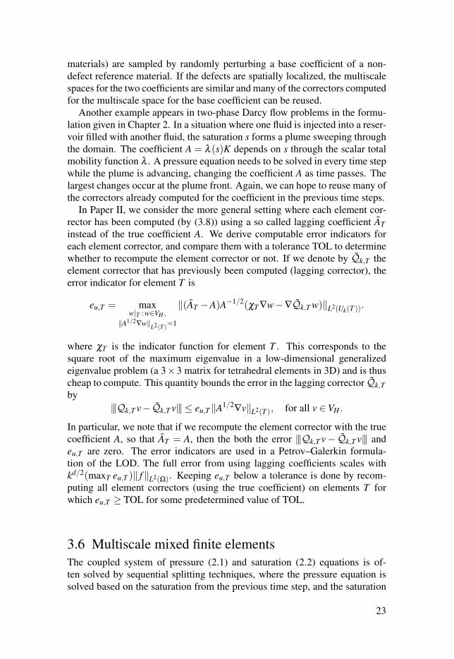
In Paper II, we consider the more general setting where each element cor-

rector has been computed (by (3.8)) using a so called lagging coefficient ATinstead of the true coefficient A. We derive computable error indicators for

each element corrector, and compare them with a tolerance TOL to determine

whether to recompute the element corrector or not. If we denote by Qk,T the

element corrector that has previously been computed (lagging corrector), the

error indicator for element T is

eu,T = maxw|T :w∈VH ,

‖A1/2∇w‖L2(T )=1

‖(AT −A)A−1/2(χT ∇w−∇Qk,T w)‖L2(Uk(T )).

where χT is the indicator function for element T . This corresponds to the

square root of the maximum eigenvalue in a low-dimensional generalized

eigenvalue problem (a 3×3 matrix for tetrahedral elements in 3D) and is thus

cheap to compute. This quantity bounds the error in the lagging corrector Qk,Tby

|||Qk,T v−Qk,T v||| ≤ eu,T‖A1/2∇v‖L2(T ), for all v ∈VH .

In particular, we note that if we recompute the element corrector with the true

coefficient A, so that AT = A, then the both the error |||Qk,T v−Qk,T v||| and

eu,T are zero. The error indicators are used in a Petrov–Galerkin formula-

tion of the LOD. The full error from using lagging coefficients scales with

kd/2(maxT eu,T )‖ f‖L2(Ω). Keeping eu,T below a tolerance is done by recom-

puting all element correctors (using the true coefficient) on elements T for

which eu,T ≥ TOL for some predetermined value of TOL.

3.6 Multiscale mixed finite elements

The coupled system of pressure (2.1) and saturation (2.2) equations is of-

ten solved by sequential splitting techniques, where the pressure equation is

solved based on the saturation from the previous time step, and the saturation

23

equation is solved using the fluxes obtained from the pressure equation at the

current time step. This procedure is iterated in time to simulate the coupled

process. Locally conservative fluxes are generally necessary for stable and ac-

curate solutions to discontinuous Galerkin or finite volume schemes used to

solve the advective transport equation (see e.g. [40] for a confirming counter

example). In the mixed form of (2.3) we seek the flux σσσ and pressure u, such

that

A−1σσσ +∇u = 0,

∇ ·σσσ = f .(3.12)

The flux σσσ is an explicit unknown that will be locally conservative if choosing

the discretization properly. The Raviart–Thomas finite element [31, 36] is one

of the most common discretizations of the flux space and it gives locally con-

servative fluxes by construction. In Paper III, we derive an a priori error bound

for an LOD method for the mixed problem (3.12) yielding locally conservative

fluxes on the coarse mesh (and the fine mesh if right hand side correction is

performed).

The weak formulation of the mixed problem uses the spaces H(div,Ω) and

H0(div,Ω) = {vvv ∈ H(div,Ω) : vvv · nnn|∂Ω = 0} where nnn is the outward facing

boundary normal. The weak formulation of a homogeneous Neumann prob-

lem reads, find σ ∈ H0(div,Ω), and u ∈ L2(Ω)/R, such that

(A−1σσσ ,vvv)− (∇ · vvv,u) = 0,

(∇ ·σσσ ,w) = ( f ,w),(3.13)

for all v ∈ H0(div,Ω), and w ∈ L2(Ω)/R. The lowest order Raviart–Thomas

finite element spaceRT H is an H0(div,Ω)-conforming discretization used for

the flux space on the mesh TH . For the pressure space, we use the space of

elementwise constants.

A multiscale method based on this discretization for Poisson’s equation on

mixed form was proposed in [30], where also a posteriori error bounds were

derived and used in an adaptive refinement algorithm. One observation from

that work is that only a multiscale space for the flux needs to be constructed

to be able to compute accurate solutions independent of fine scale variations.

The coarse elementwise constant space can be left intact. Essentially the same

method (however with a slightly different localization) is studied in Paper III,

where we derive an a priori error bound for σσσ , independent of the regularity

of σσσ and u.

A practical implementation of the method is based on a discrete full space

RT h (rather than H(div,Ω)) with very small mesh size h, resolving the fine

scale variations. The projection operator ΠH : RT h →RT H suffers from a

mild L2-instability (with respect to h→ 0), for vvvh ∈RT h with ∇ · vvvh = 0,

‖ΠHvvvh‖2L2(T ) ≤Cλ (H/h)2‖vvvh‖2

L2(T ),

24

where λ (H/h) := (1+ log(H/h))1/2 (see [42] for a proof). This affects the

the final error bound for the flux σσσmsk in the localized method,

‖A−1/2(σσσh−σσσmsk )‖L2(Ω) ≤C(H + kd/2λ (H/h)2θ k/λ (H/h))‖ f‖L2(Ω)

(3.14)

for some 0 < θ < 1 and C depending on the contrast, but not on k, h and Hor the regularity of σσσ or u. The instability can be compensated by increasing

the patch size k. For the non-localized method, the instability function does

not enter the bound at all. The effect of the instability in the localized method,

and its absence in the non-localized method, are observed in the numerical

experiments. There exist Clément type interpolation operators [1, 9, 13] for

which λ = 1 above. The paper [13] is particularly interesting from a compu-

tational point of view, since it constructs interpolation operators possessing a

necessary commuting property based on local projections. However, this re-

sult was unknown to the authors of Paper III at the time it was written, and no

numerical experiments using the operator were performed.

25

4. Estimating failure probabilities

In this chapter we study the problem of point estimation of the cumulative dis-

tribution function (cdf) for a random variable X that is an output from a model

with random input ω . We assume that the model can not be evaluated exactly,

but that approximations at different levels of accuracy can be computed. More

precisely, the problem is to find the failure probability p for a critical value yof X ,

p = Pr(X ≤ y), (4.1)

or equivalently, p = F(y) where F is the cdf of X . The inverse problem, to

determine quantile y from p is discussed in Paper V. However, since the main

contribution in that paper (selective refinement) is more easily described in

the context of estimating p, we focus on that case here. The idea of selective

refinement is to use error estimates for approximate realizations of X and refine

only realizations that can possibly affect the estimate of p, thereby avoiding

unnecessary computational work.

In the context of the two-phase Darcy flow model presented in Chapter 2,

the random input ω is the uncertain permeability field K and X is a functional

of the solutions σσσ β , sβ and uβ . We will call this functional the quantity of

interest. One example of a quantity of interest is the flux over a segment

Γ⊂ ∂Ω of the domain boundary. This flux can be expressed as the integral

X =∫

Γσσσ ·nnn, (4.2)

where nnn is the outward unit normal vector of Γ. Another example is sweep

efficiency, which is the fraction of the domain Ω that has been swept by, for

instance the non-wetting phase, at a final time T , i.e.

X = |Ω|−1∫

Ωχ(0,1](sn(T )), (4.3)

where χA is the indicator function for the set A. Throughout this work we

consider the distribution of ω as given and that it can be sampled.

The selective refinement method is applicable to stochastic integration meth-

ods for estimating expected values. Failure probabilities can be estimated by

introducing the binary variable Q = χ(−∞,y](X) and computing

p = E [Q], (4.4)

26

where E [·] denotes expected value. Note that Q attains only the values 1 and

0 with probability p and 1− p, respectively. This means there are discontinu-

ities in Q with respect to the stochastic variables. Hence, methods exploiting

smoothness or low variation of the integrand, such as sparse grids [39, 15],

lattice rules [38] and quasi-Monte Carlo [32] are not expected to perform op-

timally in general. The works in this thesis are based on Monte Carlo and

multilevel Monte Carlo [16, 20] methods. The following sections summarize

Papers IV–VI.

4.1 Monte Carlo

We introduce a hierarchy X�, �= 0,1,2, . . . of approximations of X that satisfy

the max-norm bound

|X−X�| ≤ γ �, (4.5)

for a 0 < γ < 1. The approximate failure probability Q� = χ(−∞,y](X�) can be

sampled to estimate an approximate failure probability p�=E [Q�]. If {QiL}N

i=1

is an independent sample with the same distribution as QL, then the Monte

Carlo estimator for an approximation at level �= L is

QMCN,L =

1

N

N

∑i=1

QiL.

To measure the error, we use the mean squared error, which can be split into

two terms, separating the sampling error and the numerical bias,

e[QMC

N,L

]2= E

[(QMC

N,L−E [Q])2]= N−1Var [QL]+ (E [QL−Q])2, (4.6)

where Var [·] denotes the variance. We wish this error to be less than ε2 and

require that (E [QL−Q])2 ≤ 12 ε2 and N−1Var [QL] ≤ 1

2 ε2, i.e. that the error

sources contribute equally. The bias can be bounded by the assumed max-

norm error of X� and the Lipschitz constant CF of F ,

E [QL−Q]≤ Pr(|X− y| ≤ γ L) = F(y+ γ L)−F(y− γ L)≤ 2CFγ L.

Thus, we should pick L ≈ logγ (ε) to get the desired accuracy. The variance

of a Bernoulli distribution QL with parameter pL is Var [QL] = pL(1− pL)≤ 1,

and the number of samples N is chosen proportional to ε−2 to obtain suffi-

ciently small variance. In the limit p→ 0, for so called rare events, one wants

a relative error ε/p ≤ 1. We do not specifically address this situation here.

See e.g. [2, 18, 19, 41] for methods applicable in that situation. Assuming the

following cost model

C [X�] = γ −q�,

27

for some q> 0, where C [X�] denotes the expected computational cost to com-

pute a realization of X�, the total cost of the Monte Carlo estimator is

C[QMC

N,L

]= Nγ −qL ≈ ε−2−q.

We use the notation a � b for a≤Cb for a constant C independent of ε and γ ,

and a≈ b for a � b � a. One can think of the factors ε−2 and ε−q as stemming

from the aims to reduce the sampling error and numerical bias, respectively.

4.2 Multilevel Monte CarloThe multilevel Monte Carlo (MLMC) method [16, 20] is a variance reduction

technique that uses the full hierarchy Q� (0 ≤ � ≤ L) to estimate E [QL]. It

can be interpreted as a recursive application of control variates. A new ran-

dom variable Z is formed using Q and an a priori known random variable Rcorrelated with Q and with known expected value:

Z = E [R]+Q−R.

The variance Var [Z] = Var [Q−R] is smaller than Var [Q] if Q and R are suf-

ficiently correlated. Now, Z (with lower variance) is sampled instead of Q.

A smaller sample is needed to obtain the same variance of the estimator. For

this to be beneficial, we need that (i) realizations of R are sufficiently cheap to

generate and (ii) the expected value of R is known (or can be estimated). In

the multilevel Monte Carlo method, less accurate and cheap approximations

are used as control variates for more accurate and expensive approximations.

We expand E [QL] in a telescoping sum of L levels (and level 0):

E [QL] = E [Q0]+L

∑�=1

E [Q�−Q�−1]. (4.7)

The expected values on the right hand side in (4.7) are estimated using stan-

dard MC estimators, with an individual sample size N� for each level �:

QML{N�},L =

1

N0

N0

∑i=1

Qi0 +

L

∑�=1

1

N�

N�

∑i=1

Y i� ,

where Y� = Q�−Q�−1 are called correctors. The cost estimate for MLMC

depends on the rates with which the bias E [Q�−Q] and the corrector variance

Var [Q�−Q�−1] converge with �. Under assumption (4.5), the convergence

rate for the bias is γ � according to the discussion in the previous section. See

the related work [3] for bounds of the expectation of Q�−Q given weaker

moments of X�−X . In addition to q, we assume that there is a constant b≤ 2,

so that we have|E [Q�−Q]|� γ �,

Var [Q�−Q�−1]� γ b�, for �≥ 1.

28

The sample sizes N� are determined by minimizing the expected cost with

constraint that the variance of the estimator is equal to ε2. Now if the deepest

level L is chosen to balance the numerical bias with the sampling error (as in

the Monte Carlo case), we obtain three cases for the expected cost [16],

C[QML{N�},L

]�

⎧⎪⎨⎪⎩

ε−2 q< b,ε−2(logε−1)2 q = b,ε−2−q+b q> b.

For quantities of interests computed from numerical solutions of PDEs, we are

typically in the case q> b. Optimally, the variance converges with the double

rate compared to that of the bias, i.e. b = 2. If this is the case, it is possible to

get a reduction in computational cost by a factor ε2 compared to Monte Carlo.

This is, however, not the case for the failure probability functional Q, where

the rates can be shown to be equal, i.e. b = 1. In [17], smoothness of F is

exploited to regain the optimal rate by proper smoothing of χ . In this work,

we use the max-norm error estimate (4.5) and construct an algorithm to regain

the optimal rate by reducing the expected cost of each realization.

4.3 Selective refinement

We replace the assumption (4.5) with the weaker assumption

|X−X�| ≤ γ � or |X−X�|< |X�− y| (4.8)

(see Figure 4.1) and instead introduce X ′k that we assume satisfy (4.5)

y

γ �X�

|X−X�|

|X−X�| ≤ γ �|X−X�|< |X�− y|

Figure 4.1. Illustration of condition (4.8). The numerical error is allowed to be larger

than γ � far away from y.

∣∣X−X ′k∣∣≤ γ k, (4.9)

29

Algorithm 1 Selective refinement algorithm to compute X�1: Compute X ′02: Let k = 0

3: while k < � and |X ′k− y| ≤ γ k do4: Let k = k+1

5: Compute X ′k6: end while7: Let X� = X ′k

with C[X ′k]= γ −kq as in the previous sections. Under these assumptions, it is

possible to compute X� by the algorithm in Algorithm 1. We note that the num-

ber of iterations in the selective refinement algorithm depends on the particular

realization and is thus itself a random variable. The algorithm has computa-

tional complexity C [X�]≤Cγ −�(q−1), where C depends on probability density

close to y (or in worst case Lipschitz constant CF of F). If using this algorithm

to compute X�, the results from the previous sections (again with b = 1) are

applicable with q replaced by q− 1, and we regain the the optimal rate for

large q,

C[QML{N�},L

]�

⎧⎪⎨⎪⎩

ε−2 q< 2,

ε−2(logε−1)2 q = 2,

ε−q q> 2.

The error bound (4.9) can be difficult to derive, since it needs to hold with

probability one. In a practical situation, however, it might be possible to moti-

vate a probabilistic bound that is broken only with a probability α ,

Pr(|X−X ′k| ≤ γ k)≥ 1−α, (4.10)

for each k separately. This adds a bias to E [Q�−Q] smaller than (�+1)α , so

that|E [Q�−Q]|� γ �+(�+1)α,

Var [Q�−Q�−1]� γ �+(�+1)α, for �≥ 1.(4.11)

Thus, if for a given deepest level L we pick α � (L+ 1)−1ε � (L+ 1)−1γ �,it is still possible to apply the computational complexity results above. In

Paper VI, we apply the selective refinement algorithm to a Darcy flow problem

to estimate the probability for the sweep efficiency X to be below a certain

critical value y. The number of discretization levels L was fixed to 4, and the

accuracy ε was in the order of 1 %, allowing for an α ≈ 10−3. The numerical

results showed that selective refinement can reduce the computational cost by

a factor of 5–10 in a practical example compared to multilevel and standard

Monte Carlo. The bias (�+1)α from the probabilistic bound can be reduced

to α under the assumption that the bound (4.10) holds independently of the

(random) number of iterations in the selective refinement algorithm.

30

5. Summary of papers

5.1 Paper I

F. Hellman and A. Målqvist. Contrast independent localization of multiscale

problems. ArXiv e-prints:1610.07398, 2016.

The error from localization of element correctors in the LOD method is con-

trast dependent for general choices of interpolation operators. We study an

elliptic problem with a coefficient taking one of only two possible values αand 1, with α � 1. We partition Ω into two disjoint subdomains Ω1 and Ωα

based on the value of A so that A|Ωα = α and A|Ω1 = 1. This allows for a ge-

ometrical interpretation of the coefficient in terms of the subdomains Ωα and

Ω1. We propose an interpolation operator defined in terms of the geometry of

Ω1 that gives contrast independent localization error. The construction puts

some conditions on the placement of coarse nodes in relation to the geometry

of Ω1. The implications of these conditions are studied.

ContributionsThe author of this thesis had the main responsibility for preparing the manu-

script, performed all the numerical experiments and performed most of the

analysis. The ideas were developed in close collaboration with the other au-

thor.

5.2 Paper II

F. Hellman and A. Målqvist. Numerical homogenization of time-dependent

diffusion. ArXiv e-prints:1703.08857, 2017.

We study the LOD method for a sequence of elliptic problems with simi-

lar rapidly varying coefficients. These occur for example in sample based

stochastic integration or in splitting schemes for time-dependent problems.

We define a method that constructs a multiscale space for the first coefficient

in the sequence and then adaptively updates the element correctors while step-

ping through the sequence. Computable error indicators are used to tell which

element correctors to recompute in order to keep the error below a predeter-

mined tolerance throughout the sequence of PDEs. The method automatically

exploits the decay of the element correctors to only make the necessary up-

dates.

31

ContributionsThe author of this thesis had the main responsibility for preparing the manu-

script, performed all the numerical experiments and performed most of the

analysis. The ideas were developed in close collaboration with the other au-

thor.

5.3 Paper III

F. Hellman, P. Henning, and A. Målqvist. Multiscale mixed finite elements.

Discrete Contin. Dyn. Syst. Ser. S, 9(5):1269–1298, 2016.

In this paper we derive an a priori error bound for the LOD method on Pois-

son’s equation on mixed form, based on the Raviart–Thomas finite element.

We observe that it is only necessary to construct a low-dimensional multiscale

space for the flux variable (i.e. the pressure variable needs no modification)

to get a regularity independent error bound for the flux. The flux solution is

also conservative on the coarse mesh and can be made conservative on the fine

mesh if using right hand side correction. The error bound, however, grows

logarithmically with H/h due to the L2-instability of the standard Raviart–

Thomas interpolation. Clément type interpolation operators can be used to

remove this instability.

ContributionsThe author of this thesis had the main responsibility for preparing the manu-

script, performed all the numerical experiments and performed parts of the

analysis. The ideas were developed in close collaboration with the other au-

thors.

5.4 Paper IV

D. Elfverson, D. Estep, F. Hellman, and A. Målqvist. Uncertainty quantifica-

tion for approximate p-quantiles for physical models with stochastic inputs.

SIAM/ASA J. Uncertain. Quantif., 2(1):826–850, 2014.

We develop a method for estimating p-quantiles y for outputs from a compu-

tational model with random inputs. Using computable error bounds for the

numerical error and confidence bands for the sampling error, we propose an

algorithm for computing computable lower and upper bounds, y−n,ε and y+n,ε ,

respectively, so that

Pr(y−n,ε ≤ y≤ y+n,ε)≥ 1−β ,

given a (small) probability 0 < β < 1. The algorithm (called selective refine-

ment) exploits that the accuracy of only a subset of the realizations affects the

accuracy of the estimator to reduce the computational cost. We also analyze

32

the asymptotic convergence properties of the p-quantile estimator bounds in

the limit of large sample size and decreasing numerical error.

ContributionsThe author of this thesis wrote the manuscript and performed the numerical

experiments in close collaboration with the first author. The analysis was done

by the author of this thesis, the first, and the fourth author. The ideas were

developed in close collaboration between all the authors.

5.5 Paper V

D. Elfverson, F. Hellman, and A. Målqvist. A multilevel Monte Carlo method

for computing failure probabilities. SIAM/ASA J. Uncertain. Quantif., 4(1):

312–330, 2016.

We develop a multilevel Monte Carlo method for estimating failure probabil-

ities p = Pr(X ≤ y) for a given critical value y, where X is the output from a

model with random input. Using max-norm error bounds for the error in a hi-

erarchy of increasingly expensive and accurate approximations X�, �= 0,1, . . .of X , we define an algorithm that reduces the cost complexity in terms of the

desired accuracy for the multilevel Monte Carlo method. The algorithm ex-

ploits that the accuracy of only a subset of the realizations affects the accuracy

of the estimator. This makes it possible to compute only a fraction of all real-

izations using the most accurate approximation. We prove that the asymptotic

cost in the limit of root mean square error tolerance ε → 0 is proportional to

that of computing a single approximation on the most accurate level in the

hierarchy.

ContributionsThe author of this thesis wrote the manuscript, performed the numerical ex-

periments and did the analysis in close collaboration with the first author. The

ideas were developed in close collaboration with all the authors.

5.6 Paper VI

F. Fagerlund, F. Hellman, A. Målqvist, and A. Niemi. Multilevel Monte Carlo

methods for computing failure probability of porous media flow systems. Ad-vances in Water Resources, 94:498–509, 2016.

In this paper we consider a two-phase Darcy flow system simulating an in-

jection scenario and estimate the probability for the sweep efficiency of the

injected fluid to be less than a predetermined critical value, given a probabilis-

tic model for the permeability. We use the selective refinement technique from

33

Papers IV–V in combination with standard Monte Carlo and multilevel Monte

Carlo to reduce the computational cost. Cost reductions of magnitude 5–10

are observed. We also discuss heuristics for estimating parameters required

by the methods and derive an error bound for the error introduced by using

a probabilistic bound for the approximation errors instead of the max-norm

bound assumed by the method in Paper V.

ContributionsThe author of this thesis had the main responsibility for preparing the manu-

script and performed all computations and analysis. The ideas were developed

in collaboration between all authors.

34

6. Sammanfattning på svenska

Darcys lag är en modell som beskriver hur vätskor och gaser flödar i porösa

material. Det är kanske den modell som används mest i storskaliga datorsi-

muleringar av underjordiska flöden, exempelvis spridning av föroreningar i

grundvatten, olje- och vattenflöden i oljereservoarer för utökad oljeutvinning

och flöden av saltvatten och koldioxid i salina akvifärer för koldioxidlagring.

Denna avhandling tar upp två stora utmaningar för sådana datorsimuleringar:

(i) att materialegenskaperna varierar med stor kontrast och på mycket mind-

re skala än skalan på området som beräkningen rör (snabbt varierande data)

och (ii) att materialegenskaperna till stor del är okända (osäker data). Problem

med osäker och snabbt varierande data förekommer i många andra situationer,

till exempel vid simuleringar för kompositmaterial. Trots att många av resul-

taten i denna avhandling också är tillämpbara på andra problem, diskuterar vi

resultaten i ett sammanhang av underjordiska flöden för att visa på en viktig

tillämpning.

För ett Darcy-flödesproblem tar ekvationen för trycket u ofta formen av en

elliptisk partiell differentialekvation (PDE)

−∇ ·A∇u = f ,

där f är käll- och sänktermer och koefficienten A är kopplad till permeabilite-

ten. Permeabiliteten avgör i vilken grad en vätska eller gas kan flöda genom

en viss punkt i området och den kan variera betydligt över korta avstånd på

grund av lokala variationer i berggrundens egenskaper. Den kan också variera

med flera storleksordningar när material med vitt skilda egenskaper förekom-

mer inom beräkningsområdet. Finita elementmetoden är en vanlig metod för

att lösa elliptiska ekvationer. I fallet med snabbt varierande koefficienter mås-

te dock beräkningsnätet lösa upp de fina variationerna i A för att metoden ska

ge en noggrann lösning. Ett fint nät gör att det resulterande linjära ekvations-

systemet blir mycket stort och en snabbt varierande koefficient gör det även

svårt att lösa med iterativa metoder [7, 12]. För att kunna göra storskaliga

simuleringar behöver vi minneseffektiva och parallelliserbara algoritmer.

Numerisk homogenisering eller multiskalmetoder behandlar problemet med

snabbt varierande koefficienter. En vanligt förekommande strategi är att lösa

små lokaliserade problem, vars lösning används för att konstruera en upp-

skalad operator eller modifierade basfunktioner på ett grövre nät, som sedan

ger bättre grovskaliga approximationer. I denna avhandling studerar vi loka-

liserade ortogonaluppdelningsmetoden (LOD, [27, 29]), som har sina rötter

35

i variationsmultiskalmetoden (VMS, [24]). LOD är en parallelliserbar me-

tod för att konstruera ett lågdimensionellt multiskalrum utifrån koefficienten

A med bevisbart goda approximationsegenskaper. Detta står i kontrast mot de

vanliga finita elementrummen, där man alltid kan hitta en koefficient sådan att

metoden konvergerar godtyckligt långsamt [5]. Två nära besläktade multiskal-

metoder är multiskal-finita elementmetoden [22] och nätfri polyharmonisk ho-

mogenisering [33]. Konvergensanalysen för multiskal-finita elementmetoden

bygger dock på att A är periodisk. Nätfri polyharmonisk homogenisering kan

tillämpas under svagare antaganden och de numeriska experimenten visar att

lokalisering är möjlig med bibehållen noggrannhet även för denna metod.

Vi fokuserar på tre aspekter av LOD. En aspekt är koefficienter med hög

kontrast, d.v.s. stort förhållande mellan största och minsta värde av A. Kon-

trasten ingår i feluppskattningarna för vanliga LOD som en konstant och be-

gränsar möjligheten till lokalisering. Vi gör det förenklande antagandet att A är

lika med antingen α eller 1 i varje punkt, vilket tillåter en geometrisk tolkning

av koefficienten. Vi föreslår en modifiering av LOD för kontrastoberoende

lokalisering. En annan aspekt är tidsvarierande koefficienter som förekommer

till exempel i tidsberoende tvåfas-Darcy-flödesproblem. Här konstruerar vi ett

initialt multiskalrum och härleder felindikatorer som kan tala om när och var

vi behöver uppdatera multiskalrummet för att hålla felet nere när vi stegar i

tiden. Slutligen tillämpar vi LOD på mixade finita element, mer specifikt på

Raviart–Thomas-elementet. Vi härleder a priori-feluppskattningar oberoende

av de finskaliga variationerna och erhåller en lösning som är lokalt konserva-

tiv.

Koefficienten A i tryckekvationen ovan är typsikt inte bara snabbt varie-

rande, utan även osäker. Detta har motiverat oss att utveckla och analysera

metoder för fortplantning av osäkerhet. Problemformuleringen är allmän. Vi

betraktar utdata X från en modell med slumpmässig indata ω och vi är in-

tresserade av att uppskatta felrisken p = F(y), där F är den kumulativa distri-

butionsfunktionen av X . Med andra ord, storheten X indikerar på ett fel om

X ≤ y och p är sannolikheten för detta att inträffa. Metoder för denna typ av

problem innefattar de som konstruerar en representation av X i det stokastis-

ka rummet, t.ex. första/andra ordningens pålitlighetsmetoder (FORM/SORM)

[26] och surrogatbaserade metoder (t.ex. [28]). De förstnämnda kan inte för-

väntas prestera bra om det inte finns något känt normaltillstånd från vilket

en gränspunkt för fel kan bestämmas. De senare lider av dimensionalitetens

förbannelse. Detta kan vara kritiskt för underjoriska flödesproblem där den

slumpmässiga indatan ofta är ett spatiellt slumpfält av hög stokastisk dimen-

sion. Det finns även stickprovsbaserade metoder specifikt konstruerade för att

beräkna felrisker, t.ex. delmängdssimulering [2, 41], där Markovkedje-Monte

Carlo-tekniker används för att generera stickprov koncentrerade till felhändel-

sen.

I denna avhandling betraktar vi stickprovsbaserade metoder för stokastisk

integrering. Vi fokuserar på Monte Carlo- och flernivå-Monte Carlo-metoder

36

[16] som är oberoende av representationen hos den slumpmässiga indatan. Re-

sultaten här är dock användbara också i kombination med kvasi-Monte Carlo-

metoder, gittermetoder och glesa nät, om regulariteten tillåter någon vinst av

att använda dessa. Vi betraktar det typiska fallet att enbart numeriska approx-

imationer av X är tillgängliga och att vi har möjlighet att beräkna approxi-

mationer X� för vilka felet |X −X�| avtar exponentiellt med �. Vi använder

beräkningsbara begränsningar på felet för att hitta delmängder av realisatio-

ner att beräkna på lägre approximationsnivåer och på så sätt uppnå förbättrad

komplexitetsordning för beräkningskostnaden jämfört med den vanliga Monte

Carlo-metoden och flernivå-Monte Carlo-metoden.

De tre kapitlen 2–4 ger en mer detaljerad sammanfattning av de ingående

arbetena. Kapitel 2 beskriver en modell för Darcy-flödesproblemet. Denna

modell återkommer i numeriska experiment och exempel i flera av artiklarna.

Kapitel 3 tar upp ämnet om numerisk homogenisering som täcks av artiklar-

na I–III och kapitel 4 behandlar arbetet på felriskuppskattningar som finns i

artiklarna IV–VI.

37

Acknowledgments

First of all, I want to thank my main adviser Axel Målqvist for your invaluable

support over the past five years. I have greatly appreciated your sincere inter-

est in my development as a researcher. I am particularly grateful that you have

shared with me your excellent view on computational mathematics. I would

also like to thank my co-advisers Auli Niemi and Fritjof Fagerlund for sharing

your expertise in hydrogeology and teaching me about flows in porous media.

In addition to my advisers, I want to thank my other co-authors Daniel Elfver-

son, Donald Estep, and Patrick Henning for your great contributions to our

joint efforts and for all the fun it has been working together. I would also like

to thank Daniel Peterseim, Knut-Andreas Lie, and Elisabeth Ullmann for good

discussions providing me with additional and valuable insights. It is impossi-

ble to deny that the early opportunities given to me by Kenneth Holmström set

me off on the path to this thesis. For this I am very grateful.

I thank the Centre for Interdisciplinary Mathematics, Uppsala University

for funding this thesis work. I am also grateful for generous travel grants from

Anna Maria Lundins stipendiefond, Ångpanneföreningens forskningsstiftelse,

C. F. Liljewalchs stipendiestiftelse, C. Swartz’ stiftelse, and H. F. Sederholms

stipendiestiftelse.

I have really enjoyed the friendly atmosphere at TDB and want to thank all

friends and colleagues there. So many nice people, so close to my desk. In my

view, a very good arrangement. Thank you all for making it a pleasure to go

to work! Special thanks to Martin Almquist for providing valuable comments

on a draft of this summary and for the help during the last few weeks.

To my friends, thank you for offering good advice and support during this

time. Special thanks to Olof Jönsson, David Berglund, Mikael Thuné, Ian

Wainwright, Josefin Ahlkrona, Martin Almquist, Daniel Elfverson, Patrick

Henning, Hanna Holmgren, Kalle Ljungkvist, Lina Meinecke, Slobodan Milo-

vanovic, Simon Sticko, Martin Tillenius, and Emil Nordling.

Slutligen, stort tack till mamma, Anna och Åsa för allt. Jag är så glad att

jag har er!

38

References

[1] D. N. Arnold, R. S. Falk, and R. Winther. Finite element exterior calculus,

homological techniques, and applications. Acta Numer., 15:1–155, 2006.

[2] S.-K. Au and J. L. Beck. Estimation of small failure probabilities in high

dimensions by subset simulation. Probabilistic Engineering Mechanics,

16(4):263–277, 2001.

[3] R. Avikainen. On irregular functionals of SDEs and the Euler scheme. FinanceStoch., 13(3):381–401, 2009.

[4] I. Babuška and J. E. Osborn. Generalized finite element methods: Their

performance and their relation to mixed methods. SIAM J. Numer. Anal.,20(3):510–536, 1983.

[5] I. Babuška and J. E. Osborn. Can a finite element method perform arbitrarily

badly? Math. Comp., 69(230):443–462, 2000.

[6] A. Bensoussan, J. L. Lion, and G. Papanicolaou. Asymptotic Analysis forPeriodic Structure, volume 5 of Studies in Mathematics and Its Applications.

North-Holland, Amsterdam, 1978.

[7] L. V. Branets, S. S. Ghai, S. L. Lyons, and X.-H. Wu. Challenges and

technologies in reservoir modeling. Commun. Comput. Phys., 6(1):1–23, 2009.

[8] S. C. Brenner and L. R. Scott. The Mathematical Theory of Finite ElementMethods, volume 15 of Texts in Applied Mathematics. Springer, New York, 3rd

edition, 2008.

[9] S. H. Christiansen and R. Winther. Smoothed projections in finite element

exterior calculus. Math. Comp., 77(262):813–829, 2008.

[10] P. Ciarlet. The Finite Element Method for Elliptic Problems. North-Holland,

Amsterdam, 1978.

[11] Ph. Clément. Approximation by finite element functions using local

regularization. ESAIM: Mathematical Modelling and Numerical Analysis -Modélisation Mathématique et Analyse Numérique, 9(2):77–84, 1975.

[12] B. Engquist and E. Luo. Convergence of a multigrid method for elliptic

equations with highly oscillatory coefficients. SIAM J. Numer. Anal.,34(6):2254–2273, 1997.

[13] R. S. Falk and R. Winther. Local bounded cochain projections. Math. Comp.,83:2631–2656, 2014.

[14] L. W. Gelhar. Stochastic Subsurface Hydrology. Prentice Hall, New Jersey,

1993.

[15] T. Gerstner and M. Griebel. Numerical integration using sparse grids. Numer.Algorithms, 18(3–4):209–232, 1998.

[16] M. B. Giles. Multilevel Monte Carlo path simulation. Oper. Res.,56(3):607–617, 2008.

[17] M. B. Giles, T. Nagapetyan, and K. Ritter. Multilevel Monte Carlo

approximation of distribution functions and densities. SIAM/ASA J. Uncertain.Quantif., 3(1):267–295, 2015.

39

[18] P. Glasserman, P. Heidelberger, P. Shahabuddin, and T. Zajic. Splitting for rare

event simulation: Analysis of simple cases. In Proceedings of the 1996 WinterSimulation Conference, pages 302–308, 1996.

[19] P. Glynn. Importance sampling for Monte Carlo estimation of quantiles. In

Mathematical Methods in Stochastic Simulation and Experimental Design:Proc. 2nd St. Petersburg Workshop on Simulation (Publishing House of SaintPetersburg University), pages 180–185, 1996.

[20] S. Heinrich. Multilevel Monte Carlo methods. In Large-Scale ScientificComputing, volume 2179 of Lecture Notes in Computer Science, pages 58–67.

Springer Berlin Heidelberg, 2001.

[21] P. Henning and A. Målqvist. Localized orthogonal decomposition techniques

for boundary value problems. SIAM J. Sci. Comput., 36(4):A1609–A1634,

2014.

[22] T. Y. Hou and X.-H. Wu. A multiscale finite element method for elliptic

problems in composite materials and porous media. J. Comput. Phys.,134(1):169 – 189, 1997.

[23] T.Y. Hou, X.-H. Wu, and Z. Cai. Convergence of a multiscale finite element

method for elliptic problems with rapidly oscillating coefficients. Math. Comp.,68:913–943, 1999.

[24] T. J. R. Hughes, G. R. Feijóo, L. Mazzei, and J.-B. Quincy. The variational

multiscale method—a paradigm for computational mechanics. Comput.Methods Appl. Mech. Engrg., 166(1-2):3–24, 1998.

[25] T. J. R. Hughes and G. Sangalli. Variational multiscale analysis: The fine-scale

Green’s function, projection, optimization, localization, and stabilized methods.

SIAM J. Numer. Anal., 45(2):539–557, 2007.

[26] A. Der Kiureghian. First- and second-order reliability methods. In

E. Nikolaidis, D. M. Ghiocel, and S. Singhal, editors, Engineering DesignReliability Handbook, chapter 14. CRC Press, Boca Raton, FL, 2005.

[27] M. G. Larson and A. Målqvist. Adaptive variational multiscale methods based

on a posteriori error estimation: Energy norm estimates for elliptic problems.

Comput. Methods Appl. Mech. Engrg., 196:2313–2324, 2007.

[28] Jing Li, Jinglai Li, and D. Xiu. An efficient surrogate-based method for

computing rare failure probability. J. Comput. Phys., 230(24):8683 – 8697,

2011.

[29] A. Målqvist and D. Peterseim. Localization of elliptic multiscale problems.

Math. Comp., 83(290):2583–2603, 2014.

[30] A. Målqvist. Multiscale methods for elliptic problems. Multiscale Model.Simul., 9(3):1064–1086, 2011.

[31] J. C. Nedelec. Mixed finite elements in R3. Numerische Mathematik,

35(3):315–341, 1980.

[32] H. Niederreiter. Random Number Generation and Quasi-Monte Carlo Methods.

SIAM, Philadelphia, 1992.

[33] Owhadi, H., Zhang, L., and Berlyand, L. Polyharmonic homogenization, rough

polyharmonic splines and sparse super-localization. ESAIM: M2AN,

48(2):517–552, 2014.

[34] D. Peterseim. Variational multiscale stabilization and the exponential decay of

fine-scale correctors. In G. R. Barrenechea, F. Brezzi, A. Cangiani, and E. H.

40

Georgoulis, editors, Building Bridges: Connections and Challenges in ModernApproaches to Numerical Partial Differential Equations, Lecture Notes in

Computational Science and Engineering. Springer, May 2016.

[35] D. Peterseim and R. Scheichl. Robust numerical upscaling of elliptic multiscale

problems at high contrast. Comput. Meth. in Appl. Math., 16(4):579–603, 2016.

[36] P. A. Raviart and J. M. Thomas. A mixed finite element method for 2-nd order

elliptic problems. In Ilio Galligani and Enrico Magenes, editors, MathematicalAspects of Finite Element Methods, volume 606 of Lecture Notes inMathematics, pages 292–315. Springer Berlin Heidelberg, 1977.

[37] L. R. Scott and S. Zhang. Finite element interpolation of nonsmooth functions

satisfying boundary conditions. Math. Comp., 54(190):483–493, 1990.

[38] I. H. Sloan and S. Joe. Lattice methods for multiple integration. Oxford

University Press, Oxford, 1994.

[39] S. A. Smolyak. Quadrature and interpolation formulas for tensor products of

certain classes of functions. Dokl. Akad. Nauk, 4:240–243, 1963.

[40] S. Sun and J. Liu. A locally conservative finite element method based on

piecewise constant enrichment of the continuous Galerkin method. SIAM J. Sci.Comput., 31(4):2528–2548, 2009.

[41] E. Ullmann and I. Papaioannou. Multilevel estimation of rare events.

SIAM/ASA J. Uncertain. Quantif., 3(1):922–953, 2015.

[42] B. Wohlmuth, A. Toselli, and O. Widlund. An iterative substructuring method

for Raviart–Thomas vector fields in three dimensions. SIAM J. Numer. Anal.,37(5):1657–1676, 2000.

41

Acta Universitatis UpsaliensisDigital Comprehensive Summaries of Uppsala Dissertationsfrom the Faculty of Science and Technology 1495

Editor: The Dean of the Faculty of Science and Technology

A doctoral dissertation from the Faculty of Science andTechnology, Uppsala University, is usually a summary of anumber of papers. A few copies of the complete dissertationare kept at major Swedish research libraries, while thesummary alone is distributed internationally throughthe series Digital Comprehensive Summaries of UppsalaDissertations from the Faculty of Science and Technology.(Prior to January, 2005, the series was published under thetitle “Comprehensive Summaries of Uppsala Dissertationsfrom the Faculty of Science and Technology”.)

Distribution: publications.uu.seurn:nbn:se:uu:diva-318589

ACTAUNIVERSITATIS

UPSALIENSISUPPSALA

2017