Numerical invariants through convex relaxation and max-strategy iteration
48
Form Methods Syst Des DOI 10.1007/s10703-013-0190-8 Numerical invariants through convex relaxation and max-strategy iteration Thomas Martin Gawlitza · Helmut Seidl © Springer Science+Business Media New York 2013 Abstract We present an algorithm for computing the uniquely determined least fixpoints of self-maps on R n (with R = R ∪ {±∞}) that are point-wise maximums of finitely many monotone and order-concave self-maps. This natural problem occurs in the context of sys- tems analysis and verification. As an example application we discuss how our method can be used to compute template-based quadratic invariants for linear systems with guards. The fo- cus of this article, however, lies on the discussion of the underlying theory and the properties of the algorithm itself. Keywords Fixpoint algorithms · Systems verification · Convex optimization 1 Introduction 1.1 Motivation In the context of automated verification, tight invariants are often essential for proving the correctness or the stability of given systems. Examples for systems one wants to compute tight invariants for include linear systems and linear systems with guards. Such systems are widely present in safety-critical embedded systems like aerospace control software. A typ- ical linear system without guards periodically updates its state according to a rule of the form x k+1 = Ax k + Bu k for all k ∈ N. (1) T.M. Gawlitza (B ) Carl von Ossietzky Universität Oldenburg, Oldenburg, Germany e-mail: [email protected] T.M. Gawlitza The University of Sydney, Sydney, Australia H. Seidl Technische Universität München, Munich, Germany e-mail: [email protected]
Transcript of Numerical invariants through convex relaxation and max-strategy iteration
Form Methods Syst DesDOI 10.1007/s10703-013-0190-8
Numerical invariants through convex relaxationand max-strategy iteration
Thomas Martin Gawlitza · Helmut Seidl
© Springer Science+Business Media New York 2013
Abstract We present an algorithm for computing the uniquely determined least fixpointsof self-maps on R
n(with R = R ∪ {±∞}) that are point-wise maximums of finitely many
monotone and order-concave self-maps. This natural problem occurs in the context of sys-tems analysis and verification. As an example application we discuss how our method can beused to compute template-based quadratic invariants for linear systems with guards. The fo-cus of this article, however, lies on the discussion of the underlying theory and the propertiesof the algorithm itself.
Keywords Fixpoint algorithms · Systems verification · Convex optimization
1 Introduction
1.1 Motivation
In the context of automated verification, tight invariants are often essential for proving thecorrectness or the stability of given systems. Examples for systems one wants to computetight invariants for include linear systems and linear systems with guards. Such systems arewidely present in safety-critical embedded systems like aerospace control software. A typ-ical linear system without guards periodically updates its state according to a rule of theform
xk+1 =Axk +Buk for all k ∈N. (1)
T.M. Gawlitza (B)Carl von Ossietzky Universität Oldenburg, Oldenburg, Germanye-mail: [email protected]
T.M. GawlitzaThe University of Sydney, Sydney, Australia
H. SeidlTechnische Universität München, Munich, Germanye-mail: [email protected]
Form Methods Syst Des
Here, xk ∈ Rn represents the state of the system at time k and uk the input at time k. The
matrices A and B describe, for all k ∈N, how the state xk+1 is determined from the state xk
and the input uk . To express more complicated situations, linear systems can be augmentedwith guards.
Many techniques to infer tight inductive invariants are based on the abstract interpreta-tion framework of Cousot and Cousot [6]. In its core, such techniques reduce the problemof finding tight inductive invariants to the problem of finding small solutions to inequalitiesover a well-chosen abstract domain that is a complete lattice. The abstract domain definesa set of properties that can be expressed. Each solution to the inequalities provides a soundinductive invariant. Smaller solutions to the inequalities correspond to tighter inductive in-variants, whereas greater solutions correspond to coarser inductive invariants.
The challenge is then to provide methods for computing sufficiently small, or at best,least solutions to these inequalities. The degree of difficulty of this task depends, amongother things, on the expressiveness of the abstract domain over which the inequalities areto be interpreted. It tends to be a highly non-trivial task if the abstract domain over whichthe inequalities are to be interpreted has infinite strictly ascending chains. In the latter case,the degree of difficulty obviously still depends on many factors. In the above-mentionedapplication, it is certainly more difficult to deal with an abstract domain that is capableof expressing non-linear properties than with one that is only capable of expressing linearproperties.
Linear systems and linear systems with guards, unfortunately, usually do not admit sim-ple linear inductive invariants and are thus hard to analyze. However, a remarkable propertyof linear systems which we aim to exploit is that they always admit quadratic invariants ifand only if they are stable [2]. There also always exist zonotopic approximations of suchquadratic invariants, but these approximations might be costly to compute, as the numberof faces needed may be well above the dimensionality of the system which is to be ana-lyzed [16].
The approach which we present in this article exhibits, for the case of linear systems withguards, how tight quadratic inductive invariants can be inferred, provided that a template forquadratic properties, i.e., a general layout for quadratic properties, is given before-hand. Theabstract domain for expressing quadratic properties and the quadratic inductive invariantswhich are to be inferred in particular is defined through a template. A template for quadraticproperties consists of a finite set of linear and quadratic polynomials whose variables arethe numerical variables of the program or system which is to be analyzed. The given poly-nomials define a complete lattice of expressible properties. The final goal is to compute aninductive invariant which is as tight as possible and of the shape that is defined by the tem-plate. That is, for every program point, we aim at computing safe upper bounds on the givenlinear and quadratic polynomials. We want these bounds to be as small as possible.
With appropriately chosen linear and quadratic polynomials, the abstract domain can bespecialized to intervals (the template is defined through the set of all linear polynomials xand −x for all numerical program variables x) [5], zones (the template is defined through theset of all linear polynomials x, −x, and x − y for all numerical program variables x and y)[19, 21, 30], octagons (the template is defined through the set of all linear polynomials x,−x, x− y, and x+ y for all numerical program variables x and y) [22], and, more generally,template polyhedra (the template is defined through a fixed finite set of arbitrary linearpolynomials whose variables are the numerical variables of the program or system) [26].
If we do not want to fix a template before-hand, the algorithm which is presented inthis article can be augmented with template generation methods. The resulting method can,for instance, be used to perform a fully automatic static analysis for linear systems with
Form Methods Syst Des
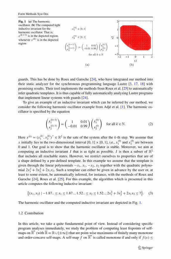
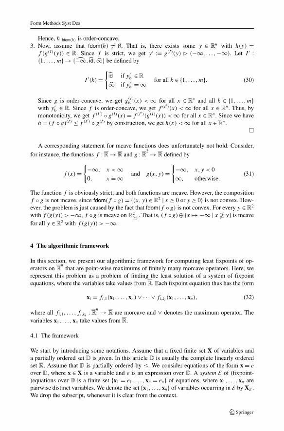
Fig. 1 (a) The harmonicoscillator. (b) The computed tightinductive invariant for theharmonic oscillator. That is,x(k+1) is in the depicted region,whenever x(k) is in the depictedregion
guards. This has be done by Roux and Garoche [24], who have integrated our method intotheir static analyzer for the synchronous programming language Lustre [3, 17, 18] withpromising results. Their tool implements the methods from Roux et al. [25] to automaticallyinfer quadratic templates. It is thus capable of fully automatically analyzing Lustre programsthat implement linear systems with guards [24].
To give an example of an inductive invariant which can be inferred by our method, weconsider the following harmonic oscillator example from Adjé et al. [1]. The harmonic os-cillator is specified by the equation
(x
(k+1)
1
x(k+1)
2
)=(
1 0.01−0.01 0.99
)(x
(k)
1
x(k)
2
)for all k ∈N. (2)
Here x(k) = (x(k)
1 , x(k)
2 )� ∈ R2 is the sate of the system after the k-th step. We assume that
x initially lies in the two-dimensional interval [0,1] × [0,1], i.e., x(0)
1 and x(0)
2 are between0 and 1. Our goal is to show that the harmonic oscillator is stable. Moreover, we aim atcomputing an inductive invariant I that is as tight as possible. I is then a subset of R
2
that includes all reachable states. However, we restrict ourselves to properties that are ofa shape defined by a pre-defined template. In this example we assume that the template isgiven through the linear polynomials −x1, x1, −x2, x2 together with the quadratic polyno-mial 2x2
1 + 3x22 + 2x1x2. Such a template can either be given in advance by the user or, at
least to some extent, be automatically inferred, for instance, with the methods of Roux andGaroche [24], Roux et al. [25]. For this example, the algorithm which is presented in thisarticle computes the following inductive invariant:
{(x1, x2) | −1.87..≤ x1 ≤ 1.87..,1.52..≤ x2 ≤ 1.52..,2x2
1 + 3x22 + 2x1x2 ≤ 7
}. (3)
The harmonic oscillator and the computed inductive invariant are depicted in Fig. 1.
1.2 Contribution
In this article, we take a quite fundamental point of view. Instead of considering specificprogram analyses immediately, we study the problem of computing least fixpoints of self-maps on R
n(with R=R∪{±∞}) that are point-wise maximums of finitely many monotone
and order-concave self-maps. A self-map f on Rn
is called monotone if and only if f (x)≤

Form Methods Syst Des
Fig. 2 (a) Graph of the function f1 with f1(x)= 12 for all x. (b) Graph of the function f2 with f2(x)=√
x
for all x. (c) Graph of the function f with f (x) = max{f1(x), f2(x)} for all x. The least fixpoint of f is 1,which is the point in which the graph of f and the graph of the identity id intersect for the first (and only)time
f (y) for all x, y ∈ Rn
with x ≤ y. Order-concavity is a generalization of concavity. Forn = 1, i.e. in the one-dimensional case, these notions coincide. A map is called concaveif and only if its hypo-graph, i.e., the set of points below the graph of the function, is aconvex set. For instance, the self-maps f1 and f2 defined by f1(x) = 1
2 and f2(x) = √x
for all x ∈R (Figs. 2(a) and 2(b), respectively) are monotone and concave. The self-map f
defined by f (x)= max{f1(x), f2(x)} for all x ∈R (Fig. 2(c)) is thus a point-wise maximumof finitely many monotone and concave self-maps. We aim at computing its least fixpoint,which is 1 in this simple example (cf. Fig. 2(c)).
Computing the least fixpoints of self-maps that are point-wise maximums of finitelymany order-concave self-maps or concave self-maps is a difficult task. Even if the self-maps are restricted to self-maps that are point-wise maximums of finitely many point-wiseminimums of finitely many linear functions, the problem is at least as hard as solving meanpayoff games [12]. The latter problem is a long outstanding problem which is in the inter-section of NP and coNP, but not known to be in P. Hence, there is little hope to solve theproblem efficiently in polynomial time, for instance through convex optimization techniquesalone.
In this article, we present a strategy improvement algorithm for computing least fixpointsof self-maps f that are point-wise maximums of finitely many monotone and order-concaveself-maps. Our algorithm performs at most exponentially many strategy improvement steps(exponential in the dimensionality). Under certain conditions, each strategy improvementstep can be performed through standard convex optimization techniques. If the self-map f
under consideration is a point-wise maximum of finitely many monotone and concave self-maps, then each strategy improvement step can be performed through solving at most lin-early many standard convex optimization problems. Depending on the class of the concaveself-maps the point-wise maximum is taken of, these convex optimization problems can befurther specialized to semi-definite or linear programming problems, for instance. Althoughit is possible to construct examples where exponentially many strategy improvement stepsare required (if the best local improvement is chosen in each step) [9], our conjecture is thatmuch less strategy improvement steps are to be performed to solve examples that stem frompractical applications. It is not known whether or not there are policies to improve strategiesthat lead to polynomial-time worst-case behaviors.
Form Methods Syst Des
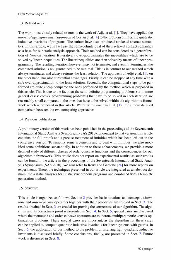
1.3 Related work
The work most closely related to ours is the work of Adjé et al. [1]. They have applied themin-strategy improvement approach of Costan et al. [4] to the problem of inferring quadraticinductive invariants of programs. The authors have also introduced a relaxed abstract seman-tics. In this article, we in fact use the semi-definite dual of their relaxed abstract semanticsas a base for our static analysis approach. Their method can be considered as a generaliza-tion of Newton iteration. It iteratively over-approximates the inequalities which are to besolved by linear inequalities. The linear inequalities are then solved by means of linear pro-gramming. The resulting iteration, however, may not terminate, and even if it terminates, thecomputed solution is not guaranteed to be minimal. This is in contrast to our method whichalways terminates and always returns the least solution. The approach of Adjé et al. [1], onthe other hand, has also substantial advantages. Firstly, it can be stopped at any time with asafe over-approximation to the least solution. Secondly, the computational steps to be per-formed are quite cheap compared the ones performed by the method which is proposed inthis article. This is due to the fact that the semi-definite programming problems (or in moregeneral cases: convex programming problems) that have to be solved in each iteration arereasonably small compared to the ones that have to be solved within the algorithmic frame-work which is proposed in this article. We refer to Gawlitza et al. [15] for a more detailedcomparison between the two competing approaches.
1.4 Previous publications
A preliminary version of this work has been published in the proceedings of the SeventeenthInternational Static Analysis Symposium (SAS 2010). In contrast to that version, this articlecontains the full proofs and a precise treatment of infinities which has been left out in theconference version. To simplify some arguments and to deal with infinities, we also mod-ified some definitions substantially. In addition to these enhancements, we provide a moredetailed study of different classes of order-concave functions and the consequences for ouralgorithmic framework. This article does not report on experimental results, as such resultscan be found in the article in the proceedings of the Seventeenth International Static Anal-ysis Symposium (SAS 2010). We also refer to Roux and Garoche [24] for more reports onexperiments. There, the techniques presented in our article are integrated as an abstract do-main into a static analyzer for Lustre synchronous programs and combined with a templategeneration method.
1.5 Structure
This article is organized as follows. Section 2 provides basic notations and concepts. Mono-tone and order-concave operators together with their properties are studied in Sect. 3. Theresults obtained in Sect. 3 are crucial for proving the correctness of our algorithm. The algo-rithm and its correctness proof is presented in Sect. 4. In Sect. 5, special cases are discussedwhere the monotone and order-concave operators are monotone multiparametric convex op-timization problems. These special cases are important, as the algorithm for these casescan be applied to compute quadratic inductive invariants for linear systems with guards. InSect. 6, the application of our method to the problem of inferring tight quadratic inductiveinvariants is discussed briefly. Some conclusions, finally, are presented in Sect. 7. Futurework is discussed in Sect. 8.
Form Methods Syst Des
2 Preliminaries
Vectors and matrices We denote the i-th row of a matrix A by Ai·. Its j -th column isdenoted by A·j . Accordingly, Ai·j denotes the component in the i-th row and the j -th col-umn. We also use these notations for vectors and vector valued functions f :X → Y k , i.e.,fi·(x)= (f (x))i· for all i ∈ {1, . . . , k} and all x ∈X.
Sets, functions, and partial functions We write A∪B for the disjoint union of two sets A
and B , i.e., A∪B stands for A ∪ B , where we assume that A ∩ B = ∅. For sets X and Y ,X → Y denotes the set of all (total) functions from X to Y , and X � Y denotes the setof all partial functions from X to Y . The domain and the co-domain of a partial functionf are denoted by dom(f ) and codom(f ), respectively. Since X → Y ⊆ X � Y ⊆ X × Y ,we apply the set operators ∪, ∩, and \ also to partial and total functions. For X′ ⊆ X, therestriction f |X′ :X′ → Y of a function f :X → Y to X′ is defined by f |X′ := f ∩X′ × Y .For f :X → Y and g :X � Y , we define f ⊕ g :X → Y by f ⊕ g := f |X\dom(g) ∪ g.
Partially ordered sets Let D be a partially ordered set (partially ordered by the binaryrelation ≤). Two elements x, y ∈D are called comparable if and only if x ≤ y or y ≤ x. Forall x ∈ D, we set D≥x := {y ∈ D | y ≥ x} and D≤x := {y ∈ D | y ≤ x}. We denote the leastupper bound and the greatest lower bound of a set X ⊆ D by
∨X and
∧X, respectively,
provided that it exists. The least element∨∅ =∧D (resp. the greatest element
∧∅ =∨D)is denoted by ⊥ (resp. �), provided that it exists. A subset C ⊆D is called a chain if and onlyif C is linearly ordered by ≤, i.e., it holds x ≤ y or y ≤ x for all x, y ∈ C. For every subsetX ⊆D of a set D that is partially ordered by ≤, we set X↑D := {y ∈D | ∃x ∈X.x ≤ y}. Theset X ⊆ D is called upward-closed w.r.t. D if and only if X↑D = X. We omit the referenceto D, whenever D is clear from the context.
Monotonicity Let D1 and D2 be partially ordered sets (partially ordered by ≤). A map-ping f : D1 → D2 is called monotone if and only if f (x) ≤ f (y) for all x, y ∈ D1 withx ≤ y. A monotone function f is called upward-chain-continuous (resp. downward-chain-continuous) if and only if f (
∨C) =∨f (C) (resp. f (
∧C) =∧f (C)) for every non-
empty chain C with∨
C ∈ dom(f ) (resp.∧
C ∈ dom(f )). It is called chain-continuous ifand only if it is both upward-chain-continuous and downward-chain-continuous.
Complete lattices A partially ordered set D is called a complete lattice if and only if∨
X
and∧
X exist for all X ⊆D. If D is a complete lattice and x ∈D, then the sub-lattices D≥x
and D≤x are also complete lattices. On a complete lattice D, we define the binary operators∨ and ∧ by
x ∨ y :=∨
{x, y}, and x ∧ y :=∧
{x, y} for all x, y ∈D. (4)
If the complete lattice D is a complete linearly ordered set (for instance R = R ∪ {±∞}),then ∨ is the binary maximum operator and ∧ the binary minimum operator. For all binaryoperators � ∈ {∨,∧}, we also consider x1 � · · · � xk as the application of a k-ary opera-tor. This will cause no problems, since the binary operators ∨ and ∧ are associative andcommutative.
Form Methods Syst Des
Fixpoints Assume that the set D is partially ordered by ≤ and f : D → D is a unaryoperator on D. An element x ∈ D is called fixpoint (resp. pre-fixpoint, resp. post-fixpoint)of f if and only if x = f (x) (resp. x ≤ f (x), resp. x ≥ f (x)). The set of all fixpoints(resp. pre-fixpoints, resp. post-fixpoints) of f is denoted by Fix(f ) (resp. PreFix(f ), resp.PostFix(f )). We denote the least (resp. greatest) fixpoint of f —provided that it exists—byμf (resp. νf ). If the partially ordered set D is a complete lattice and f is monotone, thenthe fixpoint theorem of Knaster/Tarski [28] ensures the existence of μf and νf . Moreover,it gives us that μf =∧PostFix(f ) and dually νf =∨PreFix(f ) hold.
We write μ≥xf (resp. ν≤xf ) for the least element in the set Fix(f )∩D≥x (resp. Fix(f )∩D≤x ). The existence of μ≥xf (resp. ν≤xf ) is ensured if D≥x is a complete lattice and f |D≥x
(resp. f |D≤x ) is a monotone operator on D≥x (resp. D≤x ), i.e., if D≥x (resp. D≤x ) is closedunder the operator f . The latter condition is, for instance, fulfilled if D is a complete lattice,f is a monotone operator on D, and x is a pre-fixpoint (resp. post-fixpoint) of f .
The complete lattice Rn
The set of real numbers is denoted by R, and the complete linearlyordered set R ∪ {±∞} is denoted by R. The set R
nis a complete lattice that is partially
ordered by ≤, where we write x ≤ y if and only if xi· ≤ yi· for all i ∈ {1, . . . , n}. We writex < y if and only if x ≤ y and x �= y. Additionally, we write x � y if and only if xi· < yi·for all i ∈ {1, . . . , n}. For a partial function f :Rn �R
m, we set
fdom(f ) := {x ∈ dom(f )∩Rn∣∣ f (x) ∈R
m}. (5)
The vector space Rn The standard base vectors of the Euclidean vector space R
n aredenoted by e1, . . . , en. We denote the maximum norm on R
n by ‖ · ‖, i.e., ‖x‖ = max{|xi·| |i ∈ {1, . . . , n}} for all x ∈R
n. A vector x ∈Rn with ‖x‖ = 1 is called a unit vector.
3 Monotone and order-concave operators
Order-convexity and convexity is usually defined for functions from the set Rn →R∪ {∞}.Dually, order-concavity and concavity is usually defined for functions from the set Rn →R ∪ {−∞}. For our purpose, however, we need to generalize these notions to functionsfrom the set R
n → R and finally to functions from the set Rn → R
m. We do this in this
section. We then study the properties of functions that are monotone and order-concave.The obtained results are crucial to prove the correctness of our max-strategy improvementalgorithm which is done in Sect. 4.
3.1 Monotone operators on Rn
We start our discussion with monotone operators on Rn. The main result of this subsection is
a sufficient criterion for a fixpoint of a monotone partial operator on Rn for being the great-
est pre-fixpoint.1 This criterion is important to prove the correctness of our max-strategyimprovement algorithm. To prepare this, we first show the following auxiliary lemma:
1Note that, since Rn is not a complete lattice, the greatest pre-fixpoint of f is not necessarily the greatest
fixpoint of f . The greatest fixpoint of the monotone operators f1, f2 defined by f1(x)= 12 x and f2(x)= 2x
for all x ∈R, for instance, is 0. This is also the greatest pre-fixpoint of f1, but not the greatest pre-fixpoint off2, since f2 has no greatest pre-fixpoint.
Form Methods Syst Des
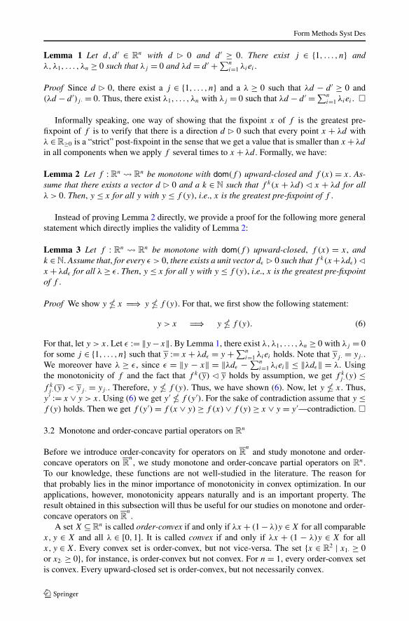
Lemma 1 Let d, d ′ ∈ Rn with d � 0 and d ′ ≥ 0. There exist j ∈ {1, . . . , n} and
λ,λ1, . . . , λn ≥ 0 such that λj = 0 and λd = d ′ +∑n
i=1 λiei .
Proof Since d � 0, there exist a j ∈ {1, . . . , n} and a λ ≥ 0 such that λd − d ′ ≥ 0 and(λd − d ′)j · = 0. Thus, there exist λ1, . . . , λn with λj = 0 such that λd − d ′ =∑n
i=1 λiei . �
Informally speaking, one way of showing that the fixpoint x of f is the greatest pre-fixpoint of f is to verify that there is a direction d � 0 such that every point x + λd withλ ∈R≥0 is a “strict” post-fixpoint in the sense that we get a value that is smaller than x+λd
in all components when we apply f several times to x + λd . Formally, we have:
Lemma 2 Let f : Rn � Rn be monotone with dom(f ) upward-closed and f (x) = x. As-
sume that there exists a vector d � 0 and a k ∈ N such that f k(x + λd) � x + λd for allλ > 0. Then, y ≤ x for all y with y ≤ f (y), i.e., x is the greatest pre-fixpoint of f .
Instead of proving Lemma 2 directly, we provide a proof for the following more generalstatement which directly implies the validity of Lemma 2:
Lemma 3 Let f : Rn � Rn be monotone with dom(f ) upward-closed, f (x) = x, and
k ∈N. Assume that, for every ε > 0, there exists a unit vector dε � 0 such that f k(x+λdε) �x + λdε for all λ≥ ε. Then, y ≤ x for all y with y ≤ f (y), i.e., x is the greatest pre-fixpointof f .
Proof We show y � x =⇒ y � f (y). For that, we first show the following statement:
y > x =⇒ y � f (y). (6)
For that, let y > x. Let ε := ‖y−x‖. By Lemma 1, there exist λ,λ1, . . . , λn ≥ 0 with λj = 0for some j ∈ {1, . . . , n} such that y := x + λdε = y +∑n
i=1 λiei holds. Note that yj · = yj ·.We moreover have λ ≥ ε, since ε = ‖y − x‖ = ‖λdε −∑n
i=1 λiei‖ ≤ ‖λdε‖ = λ. Usingthe monotonicity of f and the fact that f k(y) � y holds by assumption, we get f k
j ·(y) ≤f k
j ·(y) < yj · = yj ·. Therefore, y � f (y). Thus, we have shown (6). Now, let y � x. Thus,y ′ := x ∨ y > x. Using (6) we get y ′
� f (y ′). For the sake of contradiction assume that y ≤f (y) holds. Then we get f (y ′)= f (x ∨ y)≥ f (x)∨ f (y)≥ x ∨ y = y ′—contradiction. �
3.2 Monotone and order-concave partial operators on Rn
Before we introduce order-concavity for operators on Rn
and study monotone and order-concave operators on R
n, we study monotone and order-concave partial operators on R
n.To our knowledge, these functions are not well-studied in the literature. The reason forthat probably lies in the minor importance of monotonicity in convex optimization. In ourapplications, however, monotonicity appears naturally and is an important property. Theresult obtained in this subsection will thus be useful for our studies on monotone and order-concave operators on R
n.
A set X ⊆Rn is called order-convex if and only if λx + (1− λ)y ∈X for all comparable
x, y ∈ X and all λ ∈ [0,1]. It is called convex if and only if λx + (1 − λ)y ∈ X for allx, y ∈X. Every convex set is order-convex, but not vice-versa. The set {x ∈ R
2 | x1· ≥ 0or x2· ≥ 0}, for instance, is order-convex but not convex. For n = 1, every order-convex setis convex. Every upward-closed set is order-convex, but not necessarily convex.
Form Methods Syst Des
A partial function f :Rn �Rm is called order-convex (resp. order-concave) if and only
if dom(f ) is order-convex and
f(λx + (1− λ)y
)≤ (resp. ≥) λf (x)+ (1− λ)f (y) (7)
for all comparable x, y ∈ dom(f ) and all λ ∈ [0,1]. In fact, our notion of order-convexity isa non-standard notion. Usually, order-convexity is only defined for functions whose domainis a convex set. However, in the applications we have in mind, the generalization to order-convex domains is useful and does not do any harm. In our application non-convex butorder-convex domains like {x ∈ R
2 | x1· ≥ 0 or x2· ≥ 0} can be caused by the presence ofnon-convex guards in the program or system which is to be analyzed.
A partial function f :Rn �Rm is called convex (resp. concave) if and only if dom(f ) is
convex and
f(λx + (1− λ)y
)≤ (resp. ≥) λf (x)+ (1− λ)f (y) (8)
for all x, y ∈ dom(f ) and all λ ∈ [0,1]. Every convex (resp. concave) partial function isorder-convex (resp. order-concave), but not vice-versa.
Even convexity of the domain does not guarantee the validity of the other direction.The function f : R2 → R defined by f (x1, x2) = x1 · x2 for all x1, x2 ∈ R, for instance,has a convex domain and is order-convex.2 However, it is not convex, since, for x = (0,1),y = (1,0), and λ= 1
2 , we get f (λx+ (1−λ)y)= f ( 12 , 1
2 )= 14 > 0 = λf (x)+ (1−λ)f (y).
The restriction f |R
2≥0is monotone and order-convex, but not convex.
Note that f is (order-)concave if and only if −f is (order-)convex. Note also that f
is (order-)convex (resp. (order-)concave) if and only if fi· is (order-)convex (resp. (order-)concave) for all i = 1, . . . ,m. If n= 1, then every order-convex (resp. order-concave) partialfunction is convex (resp. concave). Every order-convex/order-concave partial function ischain-continuous. Every convex/concave partial function is continuous.
The set of (order-)convex (resp. (order-)concave) partial functions is not closed undercomposition. The functions f,g defined by f (x)= (x − 2)2 and g(x)= 1
xfor all x ∈ R>0,
for instance, are both convex and thus also order-convex. However, f ◦ g with (f ◦ g)(x)=( 1
x− 2)2 for all x ∈R>0 is neither convex nor order-convex.In contrast to the set of all order-concave partial functions, the set of all partial functions
that are both monotone and order-concave is closed under composition:
Lemma 4 Let f : Rm � Rn and g : Rl � R
m be monotone and order-convex (resp. order-concave) with codom(g) ⊆ dom(f ). The composition f ◦ g is monotone and order-convex(resp. order-concave).
Proof We assume that f and g are order-convex. The other case can be proven dually. Letx, x ′ ∈ dom(g) with x ≤ x ′, y = g(x), y ′ = g(x ′). Since g is monotone, we get y ≤ y ′. Sincef is monotone, we get (f ◦ g)(x) = f (g(x)) = f (y) ≤ f (y ′) = f (g(x ′)) = (f ◦ g)(x ′).Hence, f ◦ g is monotone.
Let λ ∈ [0,1]. Then (f ◦ g)(λx + (1− λ)x ′)= f (g(λx + (1− λ)x ′))≤ f (λg(x)+ (1−λ)g(x ′)) = f (λy + (1 − λ)y ′) ≤ λf (y) + (1 − λ)f (y ′) = λf (g(x)) + (1 − λ)f (g(x ′)) =
2The order-convexity of f can be shown as follows. Let x = (x1, x2)�, y = (y1, y2)� ∈ R2 with x ≤ y,
d = y − x, and λ ∈ [0,1]. We have d ≥ 0. We get f ((1− λ)x + λy)= f (x + λd)= (x1 + λd1)(x2 + λd2)=x1x2 +λx1d2 +λx2d1 +λ2d1d2 ≤ (1−λ)x1x2 +λx1x2 +λx1d2 +λx2d1 +λd1d2 = (1−λ)x1x2 +λ(x1 +d1)(x2 + d2)= (1− λ)f (x)+ λf (x + d)= (1− λ)f (x)+ λf (y).
Form Methods Syst Des
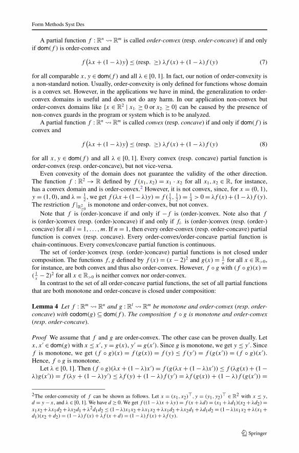
Fig. 3 Illustration for Lemma 5. The partial operator f :R�R is the point-wise minimum of an affine func-tion and the square root function and thus concave. The concavity of f ensures that x∗ + λd > f (x∗ + λd)
holds for all λ > 0 (with d := x∗ − x) provided that there exists some x < x∗ with x < f (x). Note that <
and � coincide in the one-dimensional case
λ(f ◦ g)(x)+ (1 − λ)(f ◦ g)(x ′), because f is monotone, and f and g are order-convex.Hence, f ◦ g is order-convex. �
In this subsection, our main goal is to develop a simple sufficient criterion for a fixpointof a monotone and order-concave partial operator on R
n for being the greatest pre-fixpoint.In Sect. 3.1, Lemma 2 already provides us with a sufficient criterion that can be appliedto monotone partial operators. To be able to use Lemma 2 for our purpose, we first showthe following statement that basically says that every line that (1) crosses the graph of anorder-concave function f :Rn �R at a point x∗, and (2) contains at least one point x that isbelow the graph, has the following property: all points of the open segment {x∗ +λ(x∗ −x) |λ ∈R>0} are strictly above the graph of f . Figure 3 illustrates the situation.
Lemma 5 Let f : Rn � Rn be order-convex (resp. order-concave). Let x, x∗ ∈ dom(f )
with x∗ = f (x∗), x � (resp. �) f (x), d := x∗ − x with d � 0 or d � 0. Then, x∗ + λd �(resp. �) f (x∗ + λd) for all λ > 0 with x∗ + λd ∈ dom(f ).
Proof We only consider the case that f is order-convex. The proof for the case that f isorder-concave can be carried out dually. Let λ > 0. Assume for the sake of contradictionthat there exists some i ∈ {1, . . . , n} such that (x∗ + λd)i· ≥ fi·(x∗ + λd). Since fi· is order-convex and xi· > fi·(x) holds, it follows x∗
i· > fi·(x∗)—contradiction. �
We are now prepared to prove the following sufficient criterion for a fixpoint of a mono-tone and order-concave partial operator for being the greatest pre-fixpoint. It basically saysthat a fixpoint x∗ is the greatest pre-fixpoint if we can obtain x∗ as the result of a Kleenefixpoint iteration starting from a pre-fixpoint x whose components are all strictly smallerthan the corresponding components of x∗.
Lemma 6 Let f : Rn � Rn be monotone and order-concave with dom(f ) upward-closed.
Let x∗ be a fixpoint of f , x be a pre-fixpoint of f with x � x∗, and μ≥xf = x∗. Then, x∗ isthe greatest pre-fixpoint of f .
Proof Since f is chain-continuous and x � x∗ is a pre-fixpoint of f , there exists some k ∈N
such that x � f k(x). Let x ′ be a pre-fixpoint of f . Let d := x∗ − x. Note that d � 0. Sincef k|Rn≥x
= (f |Rn≥x)k is monotone and order-concave by Lemma 4, and x∗ is a fixpoint of f k
Form Methods Syst Des
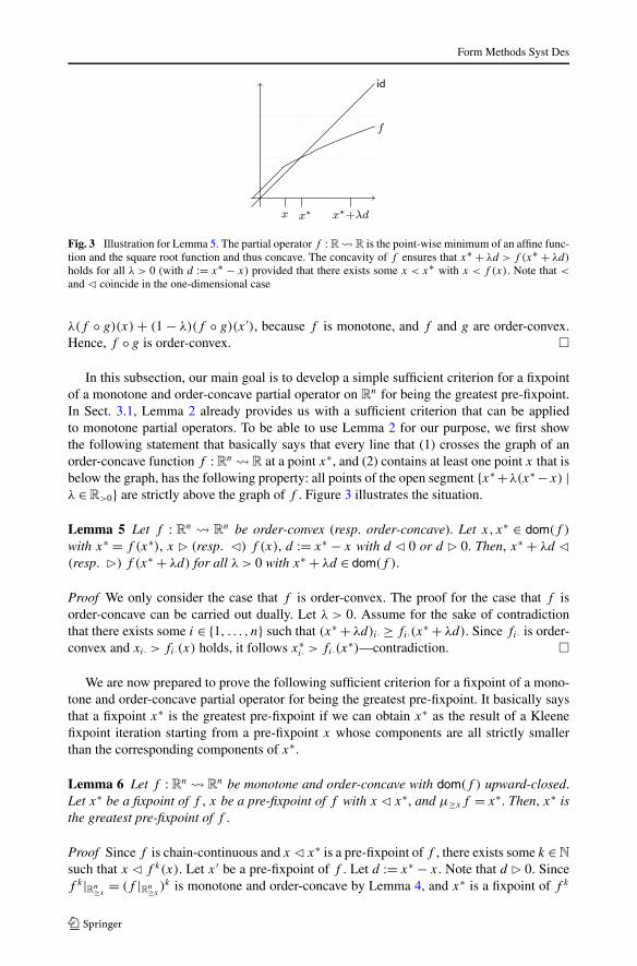
Fig. 4 The picture shows thegraph of the square root function√· :R≥0 →R. The fixpoint 1 isthe greatest pre-fixpoint. This canbe shown using Lemma 6. Thefixpoint 0 is not the greatestpre-fixpoint. In consequence,Lemma 6 cannot be applied
and thus of f k|Rn≥x, we get f k(x∗ + λd) = f k|Rn≥x
(x∗ + λd) � x∗ + λd for all λ ∈ R>0 byLemma 5. Thus, Lemma 2 gives us x ′ ≤ x∗. �
To get a better feeling for the above statement, we discuss two simple examples.
Example 1 Consider the monotone and concave partial operator√· : R� R which is de-
picted in Fig. 4. The points 0 and 1 are fixpoints of√·. Since 1
2 is a pre-fixpoint of√·,
12 < 1, and μ≥ 1
2
√· = 1, Lemma 6 gives us that 1 is the greatest pre-fixpoint of√·. Indeed,
1 is the greatest pre-fixpoint. Observe that for the fixpoint 0, there is no pre-fixpoint x ∈ R
of√· with x < 0. Therefore, Lemma 6 cannot be applied, which is no surprise since 0 is not
the greatest pre-fixpoint.
The following example shows that the criterion of Lemma 6 is sufficient, but not neces-sary:
Example 2 Let f :R→R be defined by f (x)= 0 ∧ x for all x ∈R. Recall that ∧ denotesthe minimum operator. Then, 0 is the greatest pre-fixpoint of f . However, there does notexist a x ∈ R with x < 0 such that μ≥xf = 0, since μ≥xf = x for all x ≤ 0. Therefore,Lemma 6 cannot be applied to show that 0 is the greatest pre-fixpoint of f .
In the remainder of this article, we assume that X = {x1, . . . ,xn}, where x1, . . . ,xn arepairwise distinct variables. We identify the set Rn with the set {1, . . . , n} → R and finallywith the set X → R. In consequence, we identify the set (X → R) � (X → R) with theset Rn � R
n. We use one or the other representation depending on which representation ismore convenient in the given context.
Our next goal is to weaken the preconditions of Lemma 6, i.e., we aim at providing aweaker (unfortunately also more complicated) but still sufficient criterion for a fixpoint ofa monotone and order-concave partial operator for being the greatest pre-fixpoint. Roughlyspeaking, the criterion which is provided by Lemma 6 is the right one provided that thedependency graph of the monotone and order-concave partial operator under considerationis strongly connected. If this is not the case, we sometimes (not always) have to apply thecriterion which is provided by Lemma 6 to each strongly connected component separately.Before we make this precise, we discuss an example where the dependency graph is notstrongly connected and the criterion which is provided by Lemma 6 cannot be applied. Theweaker sufficient criterion we are going to develop, however, can be applied.
Example 3 We consider the monotone and order-concave partial operator f : R2 � R2 de-
fined by f (x1, x2) := (x2 + 1 ∧ 0,√
x1) for all x1, x2 ∈ R. x∗ = (x∗1 , x∗
2 ) = (0,0) is the
Form Methods Syst Des
greatest pre-fixpoint of f . In order to prove this, assume that y = (y1, y2) > x∗ is a pre-fixpoint of f , i.e., y1 ≤ y2 + 1, y1 ≤ 0, and y2 ≤ √
y1. It follows immediately that y1 ≤ 0and thus y2 ≤√
y1 ≤√
0 = 0.Lemma 6 is not applicable to prove that x∗ is the greatest pre-fixpoint of f , simply
because there is no pre-fixpoint x of f with x � x∗. The situation is even worse: there is nox ∈ dom(f ) with x � x∗.
We observe that, locally at x∗ = (0,0), the first component f1·(x∗) of f (x∗) does notdepend on the second argument x∗
2 in the following sense: For every y = (y1, y2) ∈R2 with
y1 = x∗1 = 0 and y2 > x∗
2 = 0, we have f1·(y)= 0 = f1·(x∗). The weaker sufficient criterionwhich we develop in the following takes this into account. That is, we will assume that theset of variables can be partitioned according to their dependencies. The sufficient criterion ofLemma 6 should then hold for each partition. In this example this means: there exists somex1 < x∗
1 with x1 ≤ f1·(x1, x∗2 )= f1·(x1,0) and μ≥x1f1·(·,0)= x∗
1 = 0, and there exists somex2 < x∗
2 with x2 ≤ f2·(x∗1 , x2) = f2·(0, x2) and μ≥x2f2·(0, ·) = x∗
2 = 0. We could choosex1 = x2 =−1, for instance.
As suggested in Example 3, we partition the variables according to their dependenciesin order to derive a weaker criterion. We hence start by defining a suitable notion of depen-dency. Let X be a set of variables, f : (X →R) � (X →R) be a monotone partial operator,
and ρ : X →R be a variable assignment. For X1∪X2 = X, we write X1f,ρ→ X2 if and only if
1. X1 = ∅,2. X2 = ∅, or3. there exists an ρ ′ : X2 →R with ρ⊕ρ ′ ∈ dom(f ) and ρ ′ � ρ|X2 such that f (ρ⊕ρ ′)|X1 =
f (ρ)|X1 .
Informally speaking, X1f,ρ→ X2 states that—locally at ρ—the values of the variables from
the set X1 do not depend on the values of the variables from the set X2. Dependencies areonly admitted in the opposite direction—from X1 to X2.
Note that, because of the monotonicity of f , if condition 3 is fulfilled, then f (ρ ⊕ρ ′′)|X1 = f (ρ)|X1 for all ρ ′′ with ρ ′ ≤ ρ ′′ ≤ ρ and ρ ⊕ ρ ′′ ∈ dom(f ).
Example 4 Consider again the monotone and order-concave partial operator f : R2 � R2
from Example 3 defined by f (x1, x2) := (x2 + 1∧ 0,√
x1) for all x1, x2 ∈R. Note that f isnot a total operator, since
√x1 and thus f (x1, x2) is undefined for all x1 < 0. Let x := (0,0).
Recall that we identify the set R2 with the set {x1,x2} → R. Especially, we identify x with
the function {x1 �→ 0,x2 �→ 0}. Then, we have {x1} f,x→ {x2}. That is, locally at x, the firstcomponent f1·(x) of f (x) does not depend on the second argument x2. In other words:locally at x, one can strictly decrease the value of the second argument x2 without changingthe value of the first component f1·(x) of f (x). However, the second component f2·(x) off (x) may, locally at x, depend on the first argument x1. In this example, this is actually thecase: locally at x, we cannot decrease the value of the first argument x1 without changingthe value of the second component f2·(x) of f (x).
If the partial operator f is monotone and order-concave, then the statement X1f,ρ→ X2
also implies that, locally at ρ, the values of the X1-components of f (ρ) do not increase ifthe values of the variables from X2 increase. More formally, we have:
Form Methods Syst Des
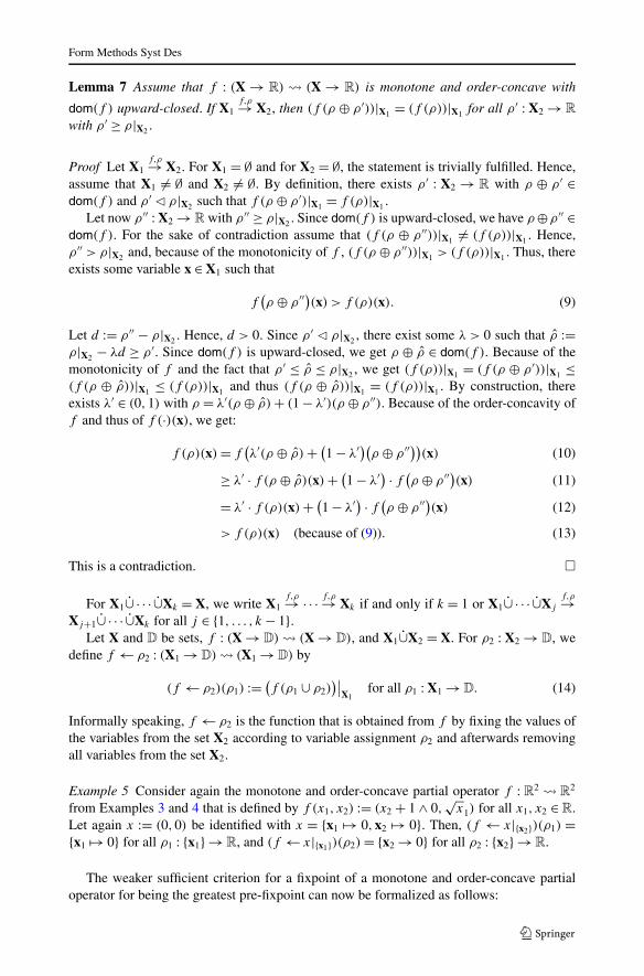
Lemma 7 Assume that f : (X → R) � (X → R) is monotone and order-concave with
dom(f ) upward-closed. If X1f,ρ→ X2, then (f (ρ ⊕ ρ ′))|X1 = (f (ρ))|X1 for all ρ ′ : X2 → R
with ρ ′ ≥ ρ|X2 .
Proof Let X1f,ρ→ X2. For X1 = ∅ and for X2 = ∅, the statement is trivially fulfilled. Hence,
assume that X1 �= ∅ and X2 �= ∅. By definition, there exists ρ ′ : X2 → R with ρ ⊕ ρ ′ ∈dom(f ) and ρ ′ � ρ|X2 such that f (ρ ⊕ ρ ′)|X1 = f (ρ)|X1 .
Let now ρ ′′ : X2 →R with ρ ′′ ≥ ρ|X2 . Since dom(f ) is upward-closed, we have ρ⊕ρ ′′ ∈dom(f ). For the sake of contradiction assume that (f (ρ ⊕ ρ ′′))|X1 �= (f (ρ))|X1 . Hence,ρ ′′ > ρ|X2 and, because of the monotonicity of f , (f (ρ ⊕ ρ ′′))|X1 > (f (ρ))|X1 . Thus, thereexists some variable x ∈ X1 such that
f(ρ ⊕ ρ ′′)(x) > f (ρ)(x). (9)
Let d := ρ ′′ − ρ|X2 . Hence, d > 0. Since ρ ′ � ρ|X2 , there exist some λ > 0 such that ρ :=ρ|X2 − λd ≥ ρ ′. Since dom(f ) is upward-closed, we get ρ ⊕ ρ ∈ dom(f ). Because of themonotonicity of f and the fact that ρ ′ ≤ ρ ≤ ρ|X2 , we get (f (ρ))|X1 = (f (ρ ⊕ ρ ′))|X1 ≤(f (ρ ⊕ ρ))|X1 ≤ (f (ρ))|X1 and thus (f (ρ ⊕ ρ))|X1 = (f (ρ))|X1 . By construction, thereexists λ′ ∈ (0,1) with ρ = λ′(ρ ⊕ ρ)+ (1− λ′)(ρ ⊕ ρ ′′). Because of the order-concavity off and thus of f (·)(x), we get:
f (ρ)(x)= f(λ′(ρ ⊕ ρ)+ (1− λ′
)(ρ ⊕ ρ ′′))(x) (10)
≥ λ′ · f (ρ ⊕ ρ)(x)+ (1− λ′) · f (ρ ⊕ ρ ′′)(x) (11)
= λ′ · f (ρ)(x)+ (1− λ′) · f (ρ ⊕ ρ ′′)(x) (12)
> f (ρ)(x) (because of (9)). (13)
This is a contradiction. �
For X1∪ · · · ∪Xk = X, we write X1f,ρ→ ·· · f,ρ→ Xk if and only if k = 1 or X1∪ · · · ∪Xj
f,ρ→Xj+1∪ · · · ∪Xk for all j ∈ {1, . . . , k − 1}.
Let X and D be sets, f : (X → D) � (X → D), and X1∪X2 = X. For ρ2 : X2 → D, wedefine f ← ρ2 : (X1 →D)� (X1 →D) by
(f ← ρ2)(ρ1) :=(f (ρ1 ∪ ρ2)
)∣∣X1
for all ρ1 : X1 →D. (14)
Informally speaking, f ← ρ2 is the function that is obtained from f by fixing the values ofthe variables from the set X2 according to variable assignment ρ2 and afterwards removingall variables from the set X2.
Example 5 Consider again the monotone and order-concave partial operator f : R2 � R2
from Examples 3 and 4 that is defined by f (x1, x2) := (x2 + 1 ∧ 0,√
x1) for all x1, x2 ∈R.Let again x := (0,0) be identified with x = {x1 �→ 0,x2 �→ 0}. Then, (f ← x|{x2})(ρ1) ={x1 �→ 0} for all ρ1 : {x1}→R, and (f ← x|{x1})(ρ2)= {x2 → 0} for all ρ2 : {x2}→R.
The weaker sufficient criterion for a fixpoint of a monotone and order-concave partialoperator for being the greatest pre-fixpoint can now be formalized as follows:

Form Methods Syst Des
Definition 1 (Feasibility) Let f : (X → R) � (X → R) be monotone and order-concavewith dom(f ) upward-closed. A fixpoint ρ∗ of f is called feasible if and only if there exist
X1∪ · · · ∪Xk = X with X1f,ρ∗→ · · · f,ρ∗→ Xk such that, for each j ∈ {1, . . . , k}, there exists some
pre-fixpoint ρ : Xj → R of f ← ρ∗|X\Xjwith ρ � ρ∗|Xj
such that μ≥ρ(f ← ρ∗|X\Xj) =
ρ∗|Xj.
Roughly speaking, feasibility means that the following two conditions are fulfilled:
1. The variables can be partitioned according to their dependencies.2. For each class of this partition, the function that is obtained by fixing the values of the
variables of the other classes fulfills the criterion which is provided by Lemma 6.
Note that any fixpoint that fulfills the criterion provided by Lemma 6 is feasible. To see this,we just have to partition the set of variables into a single set.
The following example shows that the fixpoint x = (0,0) of the previously discussedexamples is indeed feasible, although Lemma 6 cannot be applied.
Example 6 Consider again the monotone and order-concave partial operator f : R2 � R2
from the Examples 3, 4, and 5 that is defined by f (x1, x2) := (x2 + 1 ∧ 0,√
x1) for allx1, x2 ∈ R. We show that x := (0,0) is a feasible fixpoint of f . From Example 3, we knowthat Lemma 6 is not applicable to prove that x is the greatest pre-fixpoint. Recall that wecan identify the set R2 with the set {x1,x2} → R, and hence x with {x1 �→ 0,x2 �→ 0}.We have {x1} f,x→ {x2}. Moreover, {x1 �→ −1} � x|{x1} is a pre-fixpoint of f ← x|{x2} withμ≥{x1 �→−1}(f ← x|{x2})= x|{x1}, and {x2 �→ −1}� x|{x2} is a pre-fixpoint of f ← x|{x1} withμ≥{x2 �→−1}(f ← x|{x1})= x|{x2} (cf. Example 5). Thus, x is a feasible fixpoint of the mono-tone and order-concave partial operator f .
It remains to show that, for a fixpoint, feasibility is indeed sufficient for being the greatestpre-fixpoint. Since any fixpoint that fulfills the criterion which is provided by Lemma 6 isfeasible, but, as Examples 3 and 6 show, not vice-versa, the following lemma is a strictgeneralization of Lemma 6.
Lemma 8 Let f : (X → R) � (X → R) be monotone and order-concave with dom(f )
upward-closed, and ρ∗ be a feasible fixpoint of f . Then, ρ∗ is the greatest pre-fixpoint of f .
Proof Since ρ∗ is a feasible fixpoint of f , there exists X1∪ · · · ∪Xk = X with X1f,ρ∗→ · · · f,ρ∗→
Xk such that, for each j ∈ {1, . . . , k}, there exists some pre-fixpoint ρj of f ← ρ∗|X\Xjwith
ρj � ρ∗|Xjand μ≥ρj
(f ← ρ∗|X\Xj)= ρ∗|Xj
. Let ρ ′ be a pre-fixpoint of f with ρ ′ ≥ ρ∗ (it issufficient to consider this case, since the statement that ρ ′′ is a pre-fixpoint of f implies thatρ ′ := ρ∗ ∨ρ ′′ ≥ ρ∗ is also a pre-fixpoint of f ). We show by induction on j that ρ ′|X1∪···∪Xj
=ρ∗|X1∪···∪Xj
for all j ∈ {1, . . . , k}.Firstly, assume that j = 1. Since X1
f,ρ∗→ X2∪ · · · ∪Xk , Lemma 7 gives us ρ∗|X1 =(f (ρ∗))|X1 = (f ← ρ∗|X\X1)(ρ
∗|X1) = (f ← ρ ′|X\X1)(ρ∗|X1). Using the monotonicity we
thus get μ≥ρ1(f ← ρ ′|X\X1) = ρ∗|X1 . Hence, Lemma 6 gives us that ρ∗|X1 is the greatestpre-fixpoint of f ← ρ ′|X\X1 . Thus, ρ ′|X1 = ρ∗|X1 .
Now, assume that j ∈ {2, . . . , k} and ρ ′|X1∪···∪Xj−1= ρ∗|X1∪···∪Xj−1
. It remains to show
that ρ ′|Xj= ρ∗|Xj
. Since X1∪ · · · ∪Xj
f,ρ∗→ Xj+1∪ · · · ∪Xk and ρ ′|X1∪···∪Xj−1= ρ∗|X1∪···∪Xj−1
,Lemma 7 gives us that ρ∗|Xj
= (f (ρ∗))|Xj= (f ← ρ∗|X\Xj
)(ρ∗|Xj)= (f ← ρ ′|X\Xj
)(ρ∗|Xj).
Form Methods Syst Des
By monotonicity, we thus get μ≥ρj(f ← ρ ′|X\Xj
) = ρ∗|Xj. Hence, Lemma 6 gives us that
ρ∗|Xjis the greatest pre-fixpoint of (f ← ρ ′|X\Xj
). Hence ρ ′|Xj= ρ∗|Xj
. Thus, we getρ ′|X1∪···∪Xj
= ρ∗|X1∪···∪Xj. �
3.3 Monotone and order-concave operators on Rn
With the results on monotone and order-concave partial operators on Rn at hand, we are now
prepared to study total operators on Rn
that are monotone and order-concave. For that, wefirstly extend the notion of order-concavity (and hence dually the notion of order-convexity)that is defined for partial operators on R
n to total operators on Rn. Before doing so, we start
with the following observation:
Lemma 9 Let f :Rn →Rm
be monotone. Then, fdom(f ) is order-convex.
Proof Let x, y ∈ fdom(f ) with x ≤ y and λ ∈ [0,1]. Because of the monotonicity of f , weget −∞< f (x)≤ f (λx + (1− λ)y)≤ f (y) <∞. Hence, λx + (1− λ)y ∈ fdom(f ). Thisproves the statement. �
To extend the notion of (order-)convexity/(order-)concavity from Rn �R
m to Rn →R
m,
we first extend the notion of (order-)convexity/(order-)concavity from Rn � R to R
n →R as follows: let f : Rn → R, and I : {1, . . . , n} → {−∞, id,∞}. Here, −∞ denotes thefunction that assigns −∞ to every argument, id denotes the identity function, and ∞ denotesthe function that assigns ∞ to every argument. We define the mapping f (I) :Rn →R by
f (I)(x) := f(I (1)(x1·), . . . , I (n)(xn·)
)for all x ∈R
n. (15)
Hence, the function f (I) is obtained from the function f by fixing some of the arguments to−∞ respectively ∞ in accordance with I .
A function f :Rn → R is called (order-)concave if and only if the following conditionsare fulfilled for all I : {1, . . . , n}→ {−∞, id,∞}:1. fdom(f (I)) is (order-)convex.2. f (I)|fdom(f (I)) is (order-)concave. 3
3. If fdom(f (I)) �= ∅, then f (I)(x) <∞ for all x ∈Rn.
Conditions 1 and 2 state that all functions from the set Rn → R that are “contained” in thefunction f have to be (order-)concave. Condition 3 states that some form of continuity isrequired. If the function returns a finite value for some finite argument, then it is not allowedto return infinity for any finite argument.
Note that, by Lemma 9, condition 1 is fulfilled for every f : Rn → R and everyI : {1, . . . , n} → {−∞, id,∞}, whenever f is monotone. We can simplify the conditions
for functions that are monotone as follows: a monotone function f : Rn → R is order-concave if and only if the following conditions are fulfilled for all mappings I : {1, . . . , n}→{−∞, id,∞}:1. fdom(f (I)) is upward-closed w.r.t. Rn.
3Recall that, by definition of fdom, we have fdom(f (I)) ⊆ Rn and codom(f (I)|fdom(f (I ))
) ⊆ R. Hence,
f (I)|fdom(f (I ))is a function from fdom(f (I)) ⊆ R
n into R. Thus, the previously defined notion of (order-)concavity applies.

Form Methods Syst Des
2. f (I)|fdom(f (I)) is order-concave.
In order to get a better understanding for the above definition, we consider a few examples:
Example 7 Consider the operators f :R2 →R and g :R2 →R that are defined by
f (x1, x2) := √x1, g(x1, x2) :=
{√x1 if x2 <∞
x21 if x2 =∞ for all x1, x2 ∈R. (16)
f |R2 = g|R2 = {(x1, x2) �→ √x1 | x1, x2 ∈ R} is a monotone and concave operator on the
convex set fdom(f )= fdom(g)=R≥0 ×R. Nevertheless, f is monotone and order-concavewhereas g is neither monotone nor order-concave. In order to show that g is not order-concave, let I : {1,2} → {−∞, id,∞} be defined by I (1) = id and I (2) = ∞. Then,g(I)(x1, x2) = x2
1 for all x1, x2 ∈ R. Hence, fdom(g(I)) = R2. Obviously, g(I)|R2 is neither
monotone nor order-concave. Therefore, g is also not order-concave.
Some desirable properties are unfortunately not valid for order-concave functions fromthe set R
n → Rm
. The next example shows that, in contrast to the Rn → R
m case, order-concave functions are not necessarily chain-continuous. They might have a few points ofdiscontinuity.
Example 8 We consider the monotone and order-concave operator h : R2 → R which isdefined by
h(x1, x2)={√
x1 if x2 <∞√x1 + 1 if x2 =∞ for all x1, x2 ∈R. (17)
Although h is an order-concave operator on R, it is not upward-chain-continuous, since, forC = {(0, i) | i ∈R}, for instance, we have h(
∨C)= h(0,∞)= 1 > 0 =∨{0} =∨h(C).
Finally, a mapping f : Rn → Rm
is called (order-)concave if and only if fi· is (order-)concave for all i ∈ {1, . . . ,m}. A mapping f :Rn →R
mis called (order-)convex if and only
if −f is (order-)concave.One property we expect from the set of all order-concave functions from R
nin R
mis that
it is closed under the point-wise infimum operation:
Lemma 10 Let F be a set of (order-)concave functions from Rn
into Rm
. The functiong :Rn →R
mdefined by g(x) :=∧{f (x) | f ∈F} for all x ∈R
nis (order-)concave.
Proof This is straightforward. Note that g(x)= (∞, . . . ,∞) for all x ∈Rn
if F = ∅. There-fore g is concave and thus also order-concave in the latter case. �
Functions that are both monotone and order-concave play a central role in the remainderof this article. For the sake of simplicity, we give names to important classes of monotoneand order-concave functions:
Definition 2 (Morcave, Mcave, Cmorcave, and Cmcave functions) A mapping f : Rn →R
mis called morcave if and only if it is monotone and order-concave. It is called mcave if
Form Methods Syst Des
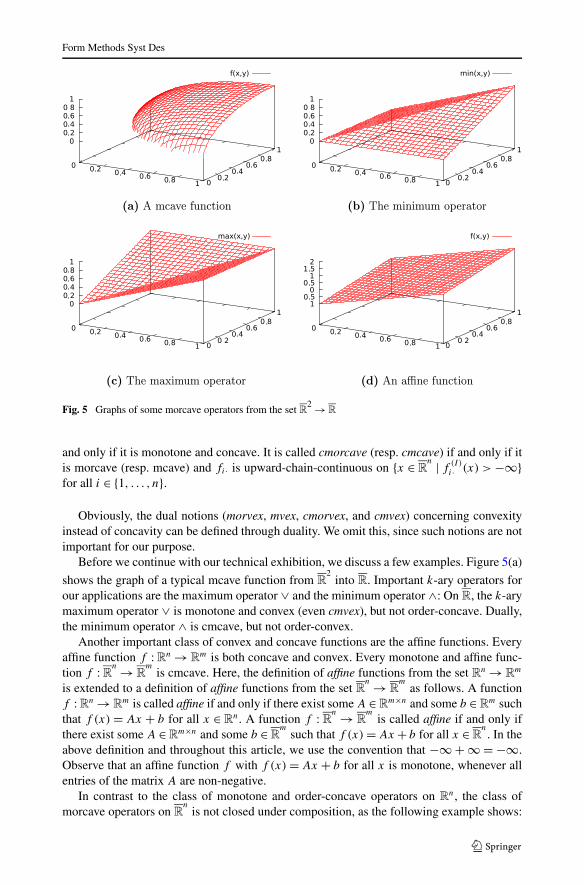
Fig. 5 Graphs of some morcave operators from the set R2 →R
and only if it is monotone and concave. It is called cmorcave (resp. cmcave) if and only if itis morcave (resp. mcave) and fi· is upward-chain-continuous on {x ∈ R
n | f (I)i· (x) > −∞}
for all i ∈ {1, . . . , n}.
Obviously, the dual notions (morvex, mvex, cmorvex, and cmvex) concerning convexityinstead of concavity can be defined through duality. We omit this, since such notions are notimportant for our purpose.
Before we continue with our technical exhibition, we discuss a few examples. Figure 5(a)
shows the graph of a typical mcave function from R2
into R. Important k-ary operators forour applications are the maximum operator ∨ and the minimum operator ∧: On R, the k-arymaximum operator ∨ is monotone and convex (even cmvex), but not order-concave. Dually,the minimum operator ∧ is cmcave, but not order-convex.
Another important class of convex and concave functions are the affine functions. Everyaffine function f :Rn →R
m is both concave and convex. Every monotone and affine func-tion f :Rn →R
mis cmcave. Here, the definition of affine functions from the set Rn →R
m
is extended to a definition of affine functions from the set Rn → R
mas follows. A function
f :Rn →Rm is called affine if and only if there exist some A ∈R
m×n and some b ∈Rm such
that f (x) = Ax + b for all x ∈ Rn. A function f : Rn → R
mis called affine if and only if
there exist some A ∈Rm×n and some b ∈R
msuch that f (x)=Ax + b for all x ∈R
n. In the
above definition and throughout this article, we use the convention that −∞+∞=−∞.Observe that an affine function f with f (x)= Ax + b for all x is monotone, whenever allentries of the matrix A are non-negative.
In contrast to the class of monotone and order-concave operators on Rn, the class of
morcave operators on Rn
is not closed under composition, as the following example shows:
Form Methods Syst Des
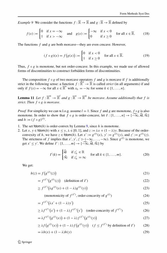
Example 9 We consider the functions f :R→R and g :R→R defined by
f (x) :={
0 if x =−∞1 if x >−∞ and g(x) :=
{−∞ if x < 0
0 if x ≥ 0for all x ∈R. (18)
The functions f and g are both morcave—they are even cmcave. However,
(f ◦ g)(x)= f(g(x)
) :={
0 if x < 0
1 if x ≥ 0for all x ∈R. (19)
Thus, f ◦ g is monotone, but not order-concave. In this example, we made use of allowedforms of discontinuities to construct forbidden forms of discontinuities.
The composition f ◦ g of two morcave operators f and g is morcave if f is additionallystrict in the following sense: a function f :Rn →R is called strict (in all arguments) if andonly if f (x)=−∞ for all x ∈R
nwith xk· = −∞ for some k ∈ {1, . . . , n}.
Lemma 11 Let f : Rm → Rl
and g : Rn → Rm
be morcave. Assume additionally that f isstrict. Then f ◦ g is morcave.
Proof For simplicity we can w.l.o.g. assume l = 1. Since f and g are monotone, f ◦g is alsomonotone. In order to show that f ◦ g is order-concave, let I : {1, . . . , n} → {−∞, id,∞}and h := (f ◦ g)(I).
1. The set fdom(h) is order-convex by Lemma 9, since h is monotone.2. Let x, y ∈ fdom(h) with x ≤ y, λ ∈ [0,1], and z := λx + (1− λ)y. Because of the order-
convexity of h, we have z ∈ fdom(h). Let x ′ := g(I)(x), y ′ := g(I)(y), and z′ := g(I)(z).The strictness of f implies that x ′, y ′, z′ � (−∞, . . . ,−∞). Since g(I) is monotone, weget x ′ ≤ y ′. We define I ′ : {1, . . . ,m}→ {−∞, id,∞} by
I ′(k)={
id if z′k· ∈R
∞ if z′k· =∞ for all k ∈ {1, . . . ,m}. (20)
We get:
h(z)= f(g(I)(z)
)(21)
= f (I ′)(g(I)(z))
(definition of I ′) (22)
≥ f (I ′)(λg(I)(x)+ (1− λ)g(I)(y))
(23)
(monotonicity of f (I ′), order-concavity of g(I)) (24)
= f (I ′)(λx ′ + (1− λ)y ′) (25)
≥ λf (I ′)(x ′)+ (1− λ)f (I ′)(y ′) (order-concavity of f (I ′)) (26)
= λf (I ′)(g(I)(x))+ (1− λ)f (I ′)(g(I)(y)
)(27)
≥ λf(g(I)(x)
)+ (1− λ)f(g(I)(y)
)(f ≤ f (I ′) by definition of I ′) (28)
= λh(x)+ (1− λ)h(y) (29)
Form Methods Syst Des
Hence, h|fdom(h) is order-concave.3. Now, assume that fdom(h) �= ∅. That is, there exists some y ∈ R
n with h(y) =f (g(I)(y)) ∈ R. Since f is strict, we get y ′ := g(I)(y) � (−∞, . . . ,−∞). Let I ′ :{1, . . . ,m}→ {−∞, id,∞} be defined by
I ′(k)={
id if y ′k· ∈R
∞ if y ′k· =∞ for all k ∈ {1, . . . ,m}. (30)
Since g is order-concave, we get g(I)k· (x) < ∞ for all x ∈ R
n and all k ∈ {1, . . . ,m}with y ′
k· ∈ R. Since f is order-concave, we get f (I ′)(x) < ∞ for all x ∈ Rn. Thus, by
monotonicity, we get f (I ′) ◦ g(I)(x)= f (I ′)(g(I)(x)) <∞ for all x ∈ Rn. Since we have
h= (f ◦ g)(I) ≤ f (I ′) ◦ g(I) by construction, we get h(x) <∞ for all x ∈Rn.
�
A corresponding statement for mcave functions does unfortunately not hold. Consider,
for instance, the functions f :R→R and g :R2 →R defined by
f (x)={−∞, x <∞0, x =∞ and g(x, y)=
{−∞, x, y < 0
∞, otherwise.(31)
The function f is obviously strict, and both functions are mcave. However, the compositionf ◦ g is not mcave, since fdom(f ◦ g)= {(x, y) ∈R
2 | x ≥ 0 or y ≥ 0} is not convex. How-ever, the problem is just caused by the fact that fdom(f ◦ g) is not convex. For every y ∈R
2
with f (g(y)) >−∞, f ◦g is mcave on R2≥y . That is, (f ◦g)⊕{x �→ −∞ | x � y} is mcave
for all y ∈R2 with f (g(y)) >−∞.
4 The algorithmic framework
In this section, we present our algorithmic framework for computing least fixpoints of op-erators on R
nthat are point-wise maximums of finitely many morcave operators. Here, we
represent this problem as a problem of finding the least solution of a system of fixpointequations, where the variables take values from R. Each fixpoint equation thus has the form
xi = fi,1(x1, . . . ,xn)∨ · · · ∨ fi,ki(x1, . . . ,xn), (32)
where all fi,1, . . . , fi,ki: Rn → R are morcave and ∨ denotes the maximum operator. The
variables x1, . . . ,xn take values from R.
4.1 The framework
We start by introducing some notations. Assume that a fixed finite set X of variables anda partially ordered set D is given. In this article D is usually the complete linearly orderedset R. Assume that D is partially ordered by ≤. We consider equations of the form x = e
over D, where x ∈ X is a variable and e is an expression over D. A system E of (fixpoint-)equations over D is a finite set {x1 = e1, . . . ,xn = en} of equations, where x1, . . . ,xn arepairwise distinct variables. We denote the set {x1, . . . ,xn} of variables occurring in E by XE .We drop the subscript, whenever it is clear from the context.

Form Methods Syst Des
For a variable assignment ρ : X → D, an expression e is mapped to a value [[e]]ρ bysetting [[x]]ρ := ρ(x), and [[f (e1, . . . , ek)]]ρ := f ([[e1]]ρ, . . . , [[ek]]ρ), where x ∈ X, f is ak-ary operator (k = 0 is possible; then f is a constant), for instance +, and e1, . . . , ek areexpressions. For every system E of equations, we define the unary operator [[E]] on X →D
by setting ([[E]]ρ)(x) := [[e]]ρ for all equations x = e from E and all ρ : X →D. A solutionis a fixpoint of [[E]], i.e., it is a variable assignment ρ such that ρ = [[E]]ρ. We denote the setof all solutions of E by Sol(E).
The set X → D of all variable assignments is a complete lattice. For ρ,ρ ′ : X → D, wewrite ρ � ρ ′ (resp. ρ � ρ ′) if and only if ρ(x) < ρ ′(x) (resp. ρ(x) > ρ ′(x)) for all x ∈ X. Ford ∈ D, d denotes the variable assignment {x �→ d | x ∈ X}. A variable assignment ρ with⊥ � ρ � � is called finite. A pre-solution (resp. post-solution) is a variable assignment ρ
such that ρ ≤ [[E]]ρ (resp. ρ ≥ [[E]]ρ) holds. The set of pre-solutions (resp. the set of post-solutions) is denoted by PreSol(E) (resp. PostSol(E)). The least solution (resp. the greatestsolution) of a system E of equations is denoted by μ[[E]] (resp. ν[[E]]), provided that it exists.For a pre-solution ρ (resp. for a post-solution ρ), μ≥ρ[[E]] (resp. ν≤ρ[[E]]) denotes the leastsolution that is greater than or equal to ρ (resp. the greatest solution that is less than or equalto ρ).
An expression e (resp. a (fixpoint-)equation x = e is called monotone if and only if [[e]]is monotone. In our setting, the fixpoint theorem of Knaster/Tarski can be stated as follows:every system E of monotone fixpoint equations over a complete lattice has a least solu-tion μ[[E]] and a greatest solution ν[[E]]. Furthermore, we have μ[[E]] =∧PostSol(E) andν[[E]] =∨PreSol(E).
Definition 3 (∨-morcave equations) An expression e (resp. fixpoint equation x = e) overR is called morcave (resp. cmorcave, resp. mcave, resp. cmcave) if and only if [[e]] is mor-cave (resp. cmorcave, resp. mcave, resp. cmcave). An expression e (resp. fixpoint equationx = e) over R is called ∨-morcave (resp. ∨-cmorcave, resp. ∨-mcave, resp. ∨-cmcave) ifand only if e = e1 ∨ · · · ∨ ek , where e1, . . . , ek are morcave (resp. cmorcave, resp. mcave,resp. cmcave).
Example 10 The square root operator√· : R→ R (defined by
√x := sup{y ∈ R | y2 ≤ x}
for all x ∈ R) is cmcave. E = {x = 12 ∨
√x} is thus a system of ∨-cmcave equations whose
least solution μ[[E]] is {x �→ 1}.
An important notion for our purpose is the notion of ∨-strategies that we define as fol-lows: A ∨-strategy σ for a system E of equations is a function that maps every right-handside e1 ∨· · ·∨ ek of E to one of the immediate sub-expressions ej , j ∈ {1, . . . , k}. We denotethe set of all ∨-strategies for E by ΣE . We drop the subscript, whenever it is clear from thecontext. The application E(σ ) of σ to E is defined by E(σ ) := {x = σ(e) | x = e ∈ E}.
Example 11 The two ∨-strategies σ1 and σ2 for the system E of ∨-cmcave equations whichis defined in Example 10 lead to the systems E(σ1) = {x = 1
2 } and E(σ2) = {x = √x} of
cmcave equations.
We now present our ∨-strategy improvement algorithm in a general setting. That is, weconsider arbitrary systems of monotone equations over arbitrary complete linearly orderedsets D. The algorithm iterates over ∨-strategies. It maintains a current ∨-strategy σ and acurrent approximate to the least solution ρ. A so-called ∨-strategy improvement operatoris used to determine a next, improved ∨-strategy σ ′. Whether or not a ∨-strategy σ ′ is an
Form Methods Syst Des
improvement of the current ∨-strategy σ may depend on the current approximate to the leastsolution ρ:
Let E be a system of monotone equations over a complete linearly ordered set. Letσ,σ ′ ∈Σ be ∨-strategies for E and ρ be a pre-solution of E(σ ). The ∨-strategy σ ′ is calledan improvement of σ w.r.t. ρ if and only if the following conditions are fulfilled:
1. If ρ ∈ Sol(E), then σ ′ = σ .2. If ρ /∈ Sol(E), then [[E(σ ′)]]ρ > ρ.3. For all equations x = e of E with [[σ ′(e)]]ρ = [[σ(e)]]ρ, we have σ ′(e)= σ(e).
An improvement σ ′ of σ w.r.t. ρ with σ ′ �= σ is called a strict improvement. A functionP∨ that assigns an improvement of σ w.r.t. ρ to every pair (σ,ρ), where σ is a ∨-strategyand ρ is a pre-solution of E(σ ), is called a ∨-strategy improvement operator.
Example 12 Consider the system E = {x1 = x2 +1∧ 0,x2 =−1∨√x1} of ∨-cmcave equa-
tions. Let σ1 and σ2 be the ∨-strategies for E such that
E(σ1)= {x1 = x2 + 1∧ 0,x2 =−1}, and (33)
E(σ2)= {x1 = x2 + 1∧ 0,x2 =√
x1}. (34)
The variable assignment ρ := {x1 �→ 0,x2 �→ −1} is a solution and thus also a pre-solutionof E(σ1). The ∨-strategy σ2 is an improvement of the ∨-strategy σ1 w.r.t. ρ.
The algorithm is parametrized with a ∨-strategy improvement operator P∨. The input isa system E of monotone equations over a complete linearly ordered set, an initial ∨-strategyσinit for E , and an initial pre-solution ρinit of E(σinit). In order to compute the least and notjust some solution, we additionally require that ρinit ≤ μ[[E]] holds:
Algorithm 1 The ∨-Strategy Improvement Algorithm
Parameter: A ∨-strategy improvement operator P∨
Input:⎧⎨⎩
A system E of monotone equations over a complete linearly ordered setA ∨-strategy σinit for EA pre-solution ρinit of E(σinit) with ρinit ≤ μ[[E]]
Output: The least solution μ[[E]] of E
σ ← σinit;ρ ← ρinit;while(ρ /∈ Sol(E)){
σ ← P∨(σ,ρ);ρ ← μ≥ρ[[E(σ )]];
}return ρ;
For the correctness of the algorithm, it is not important with which ∨-strategy improve-ment operator the algorithm is parametrized. However, some ∨-strategy improvement oper-ators may lead to fewer ∨-strategy improvement steps than others. One natural choice for a∨-strategy improvement operator is the one that always chooses a locally best improvement.
Form Methods Syst Des
That is, among the ∨-strategies it chooses an improvement σ ′ such that [[E(σ ′)]]ρ = [[E]]ρ.However, although this is a good choice in practice, there are contrived classes of examplesthat require exponentially many ∨-strategy improvement steps with this choice [9]. A deepstudy of how to choose a good ∨-strategy improvement operator is out of scope of thisarticle and remains for future work.
It remains to explain how we can compute μ≥ρ[[E(σ )]] in each improvement step. Thisstep is called value determination. We also have to show that the algorithm returns the cor-rect answer whenever it terminates. As stated by Lemma 12 below, the latter easily followsfrom the definitions by a straight-forward induction. How to compute μ≥ρ[[E(σ )]] dependson the class of equation systems under consideration. As we will see, in our case, i.e. forsystems of ∨-morcave equations, we can perform this step (under certain circumstances) bysolving convex optimization problems. We will further see that in this case the algorithmis guaranteed to terminate—assuming that we can solve the occurring convex optimizationproblems precisely.4 More precisely, it returns the least solution at the latest after consid-ering every ∨-strategy at most |X| times. That is, it terminates after at most exponentiallymany strategy improvement steps. Our conjecture is that for most practical cases much lessstrategy improvement steps are necessary.
Lemma 12 Let E be a system of monotone equations over a complete linearly ordered set.For all i ∈N, let ρi be the value of the program variable ρ and σi be the value of the programvariable σ in the ∨-strategy improvement algorithm (Algorithm 1) after the i-th evaluationof the loop-body. The following statements hold for all i ∈N:
1. ρi ≤ μ[[E]].2. ρi ∈ PreSol(E(σi+1)).3. If ρi < μ[[E]], then ρi+1 > ρi .4. If ρi = μ[[E]], then ρi+1 = ρi .
The algorithm computes the least solution, whenever it terminates.
Before we continue with our technical exhibition, we consider an example.
Example 13 We consider the system
E ={
x =−∞∨ 12 ∨
√x∨ 7
8 +√
x− 4764
}(35)
of ∨-cmorcave equations. We start with the ∨-strategy σ0 that leads to the system
E(σ0)= {x =−∞} (36)
of cmorcave equations. Then ρ0 := −∞ is a feasible solution of E(σ0). Since ρ0 /∈ Sol(E),we improve σ0 w.r.t. ρ0 to the ∨-strategy σ1 that gives us
E(σ1)={x = 1
2
}. (37)
4The assumption that we can solve all occurring convex optimization problems precisely is not realistic inpractice. In practice one has to take numerical issues into account. However, this is beyond the scope of thisarticle.
Form Methods Syst Des
Then, ρ1 := μ≥ρ0 [[σ1]] = {x �→ 12 }. Since
√12 > 1
2 and 78 +
√12 − 47
64 < 12 hold, we improve
the strategy σ1 w.r.t. ρ1 to the ∨-strategy σ2 with
E(σ2)={x =√
x}. (38)
We get ρ2 := μ≥ρ1 [[σ2]] = {x �→ 1}. Since
78 +
√1− 47
64 > 78 +
√1− 60
64 = 98 > 1,
we get σ3 = {x = 78 +
√x− 47
64 }. Finally we get ρ3 := μ≥ρ2 [[σ3]] = {x �→ 2}. The algorithmterminates, because ρ3 solves E . Therefore, ρ3 = μ[[E]]. As we will see subsequently, ρ1,ρ2, and ρ3 can be computed through convex optimization.
4.2 Feasibility
In this subsection, we extend our notion of feasibility as introduced by Definition 1. Wethen show that feasibility is preserved during the execution of Algorithm 1, whenever thealgorithm is started in the feasible region. In the next subsection, we finally utilize this factto prove termination and implement the value determination step.
We denote by E[x1/X1, . . . , xk/Xk] the equation system that is obtained from the equa-tion system E by simultaneously replacing, for all i ∈ {1, . . . , k}, every occurrence of avariable from the set Xi in the right-hand sides of E by the value xi . Here, we assume thatX1, . . . ,Xk ⊆ X are disjunct sets of variables.
Definition 4 (Feasibility) Let E be a system of morcave equations. A finite solution ρ of Eis called (E-)feasible if and only if ρ is a feasible fixpoint of [[E]]. A pre-solution ρ of E with[[E]]ρ � −∞ is called (E-)feasible if and only if ρ ′|X′ is a feasible finite solution of E ′ :={x = e ∈ E | x ∈ X′}[∞/(X \ X′)], where ρ ′ := μ≥ρ[[E]] and X′ := {x ∈ X | ρ ′(x) < ∞}.A pre-solution ρ of E is called feasible if and only if e = −∞ for all equations x = e ∈ Ewith [[e]]ρ =−∞, and ρ|X′ is a feasible pre-solution of E ′ := {x = e ∈ E | x ∈ X′}[−∞/(X\X′)], where X′ := {x | x = e ∈ E, [[e]]ρ >−∞}.
Before we continue, we consider two examples:
Example 14 We consider the system E = {x =√x} of mcave equations. For all x ∈ R, let
x := {x �→ x}. From Example 1, we know that the solution 0 is not feasible, whereas thesolution 1 is feasible. Thus, x is a feasible pre-solution for all x ∈ (0,1]. Note that 1 is theonly feasible finite solution of E and thus, by Lemma 8, the greatest finite pre-solution of E .
Example 15 Consider the system E = {x1 = x2 + 1 ∧ 0,x2 = √x1} of mcave equations.
From Example 6 it follows that ρ := {x1 �→ 0,x2 �→ 0} is a feasible finite fixpoint of [[E]].Thus, {x1 �→ 0,x2 �→ x} is a feasible pre-solution for all x ∈ [−1,0]. The solution {x1 �→−∞,x2 �→ −∞} is not feasible, since the right-hand sides evaluate to −∞, although theyare not equal to the constant −∞.
The following two lemmas imply that our ∨-strategy improvement algorithm stays in thefeasible region, whenever it is started in the feasible region. In a first step, we make sure thatthe value determination step preserves feasibility:
Form Methods Syst Des
Lemma 13 Let E be a system of morcave equations and ρ be a feasible pre-solution of E .All pre-solutions ρ ′ of E with ρ ≤ ρ ′ ≤ μ≥ρ[[E]] are feasible.
Proof The statement is an immediate consequence of the definition. �
It remains to ensure that improving strategies preserves feasibility. This is, unfortunately,quite technical to prove.
Lemma 14 Let E be a system of ∨-morcave equations, σ be a ∨-strategy for E , ρ be afeasible solution of E(σ ), and σ ′ be an improvement of σ w.r.t. ρ. Then, ρ is a feasiblepre-solution of E(σ ′).
Proof Let ρ∗ := μ≥ρ[[E(σ ′)]]. We assume w.l.o.g. that −∞ � ρ∗ � ∞. We can do sow.l.o.g. since we can otherwise remove the variables that are mapped to −∞ or ∞ by ρ∗. Itfollows that ρ �∞. Let
Xold := {x ∈ X | ρ(x) >−∞}, and (39)
Eold := {x = e ∈ E(σ ) | x ∈ Xold}[−∞/
(X \Xold
)]. (40)
Hence, by definition, ρ|Xold is a feasible finite solution of Eold, i.e., a feasible finite fixpointof [[Eold]]. Therefore, there exist X1∪ · · · ∪Xk = Xold with
X1
[[Eold]],ρ|Xold→ ·· · [[Eold]],ρ|Xold→ Xk (41)
such that, for each j ∈ {1, . . . , k}, there exists some pre-fixpoint ρ ′ of [[Eold]] ← ρ|Xold\Xj
with ρ ′ � ρ|Xjsuch that μ≥ρ′([[Eold]]← ρ|Xold\Xj
)= ρ|Xj.
Let Ximp := {x ∈ X | ρ∗(x) > ρ(x)}, X′j := Xj \ Ximp for all j ∈ {1, . . . , k}, and X′
k+1 :=Ximp. By construction, we have X′
1∪ · · · ∪X′k+1 = X. It remains to show that the following
properties are fulfilled:
1. X′1[[E(σ ′)]],ρ∗→ · · · [[E(σ ′)]],ρ∗→ X′
k+12. For each j ∈ {1, . . . , k + 1}, there exists some pre-fixpoint ρ ′ with ρ ′ � ρ∗|X′
jsuch that
μ≥ρ′([[E(σ ′)]]← ρ∗|X\X′j)= ρ∗|X′
j.
In order to prove statement 1, let j ∈ {1, . . . , k}. We have to show that
X′1∪ · · · ∪X′
j
[[E(σ ′)]],ρ∗→ X′j+1∪ · · · ∪X′
k+1. (42)
Since X1∪ · · · ∪Xj
[[Eold]],ρ|Xold→ Xj+1∪ · · · ∪Xk , there exists some variable assignment ρ ′ :Xj+1∪ · · · ∪Xk →R with ρ ′ � ρ|Xj+1∪···∪Xk
such that
([[Eold]](
ρ|Xold ⊕ ρ ′))∣∣X1∪···∪Xj
= ([[Eold]](ρ|Xold)
)∣∣X1∪···∪Xj
. (43)
We define ρ ′′ : X′j+1∪ · · · ∪X′
k+1 →R by
ρ ′′(x)=
⎧⎪⎨⎪⎩
ρ ′(x) if x ∈ X′j+1∪ · · · ∪X′
k
ρ(x) if x ∈ X′k+1 and x ∈ Xold
ρ∗(x)− 1 if x ∈ X′k+1 and x /∈ Xold
for all x ∈ X′j+1∪ · · · ∪X′
k+1.
Form Methods Syst Des
By construction, we have ρ ′′ � ρ∗|X′j+1∪···∪X′
k+1. Hence, we get
([[E(σ ′)]](ρ∗))|X′
1∪···∪X′j≥ ([[E(σ ′)]](ρ∗ ⊕ ρ ′′))|X′
1∪···∪X′j
(ρ∗ ≥ ρ∗ ⊕ ρ ′′)
≥ ([[Eold]](
ρ|Xold ⊕ ρ ′))|X′1∪···∪X′
j
= ([[Eold]](ρ|Xold)
)|X′1∪···∪X′
j(because of (43))
= ([[Eold]](
ρ∗|Xold
))|X′1∪···∪X′
j(because of Lemma 7)
= ([[E(σ ′)]](ρ∗))|X′1∪···∪X′
j.
Thus, ([[E(σ ′)]](ρ∗ ⊕ ρ ′′))|X′1∪···∪X′
j= ([[E(σ ′)]](ρ∗))|X′
1∪···∪X′j. This proves statement 1.
In order to prove statement 2, let j ∈ {1, . . . , k + 1}. We distinguish 2 cases. Firstly, as-sume that j ≤ k. Since ρ|Xold is a feasible finite fixpoint of [[Eold]], there exists some pre-fixpoint ρ ′ with ρ ′ � ρ|Xj
= ρ∗|Xjsuch that μ≥ρ′([[Eold]] ← ρ|Xold\Xj
) = ρ|Xj= ρ∗|Xj
.Using monotonicity, we get μ≥ρ′([[Eold]] ← ρ∗|Xold\Xj
) = ρ|Xj= ρ∗|Xj
. Hence, ρ ′|X′j:
X′j → R, ρ ′|X′
j� ρ|X′
j= ρ∗|X′
j, and μ≥ρ′ |X′
j
([[Eold]] ← ρ∗|Xold\X′j) = μ≥ρ′|X′
j
([[E(σ ′)]] ←ρ∗|X\X′
j)= ρ∗|X′
j. This proves statement 2 for j ≤ k. Now, assume that j = k+1. By defini-
tion of X′k+1, ρ|X′
k+1� ρ∗|X′
k+1. Moreover, we get immediately that ρ|X′
k+1is a pre-fixpoint of
[[E(σ ′)]]← ρ∗|X\X′k+1
and μ≥ρ|X′k+1
([[E(σ ′)]]← ρ∗|X\X′k+1
)= ρ∗|X′k+1
. This proves statement
2. �
Example 16 We continue Example 12. That is, we consider the equation system E = {x1 =x2 + 1 ∧ 0,x2 = −1 ∨ √
x1}. Obviously, ρ = {x1 �→ 0,x2 �→ −1} is a feasible solution ofE(σ1)= {x1 = x2 + 1∧ 0,x2 =−1}. The ∨-strategy σ2 with E(σ2)= {x1 = x2 + 1∧ 0,x2 =√
x1} is an improvement of the ∨-strategy σ1 w.r.t. ρ. By Lemma 14, ρ is also a feasiblepre-solution of E(σ2). The fact that ρ is a feasible pre-solution of E(σ2) is also shown inExample 15.
Our definition of an improvement σ ′ of a ∨-strategy σ w.r.t. ρ requires that, for allequations x = e of E , σ ′(e)= σ(e) whenever [[σ ′(e)]]ρ = [[σ(e)]]ρ. The following exampleshows that this requirement is necessary to ensure that feasibility is preserved by improve-ment steps:
Example 17 Consider the equation system E = {x1 = 0∨ x1}. Assume that E(σ )= {x1 = 0}and E(σ ′) = {x1 = x1}. The variable assignment ρ := {x1 �→ 0} is a feasible solution ofE(σ ). If we omitted the third requirement of the definition of improvements, then σ ′ wouldbe an improvement of σ w.r.t. ρ. However, as it can be easily verified, ρ is not a feasiblepre-solution of E(σ ′).
The initial ∨-strategy Lemmas 13 and 14 ensure that our ∨-strategy improvement algo-rithm stays in the feasible region, whenever it is started in the feasible region. In order tostart in the feasible region, in the following we simply assume w.l.o.g. that each equation ofE is of the form x =−∞∨ e. We say that such a system of fixpoint equations is in standardform. Then, we start our ∨-strategy improvement algorithm with a ∨-strategy σinit such that
E(σinit)= {x =−∞ | x ∈ X}. (44)
Form Methods Syst Des
In consequence, ρinit =−∞ is a feasible solution of E(σinit). The algorithm can therefore bestarted in the feasible region with σinit and ρinit. We get:
Lemma 15 Let E be a system of ∨-morcave equations in standard form. For all i ∈N, let ρi
be the value of the program variable ρ and σi be the value of the program variable σ in the∨-strategy improvement algorithm (Algorithm 1) after the i-th evaluation of the loop-body.Then, for all i ∈N, ρi and thus ρi+1 are feasible pre-solutions of E(σi+1).
Example 18 We again consider the system
E = {x1 =−∞∨ x2 + 1∧ 0,x2 =−∞∨−1∨√x1}
(45)
of ∨-morcave equations which have been introduced in Example 12. A run of our ∨-strategyimprovement algorithm gives us
E(σ0)= {x1 =−∞,x2 =−∞}, ρ0 = {x1 �→ −∞,x2 �→ −∞}, (46)
E(σ1)= {x1 =−∞,x2 =−1}, ρ1 = {x1 �→ −∞,x2 �→ −1}, (47)
E(σ2)= {x1 = x2 + 1∧ 0,x2 =−1}, ρ2 = {x1 �→ 0,x2 �→ −1}, (48)
E(σ3)={x1 = x2 + 1∧ 0,x2 =√
x1
}, ρ3 = {x1 �→ 0,x2 �→ 0}. (49)
By Lemma 15, for all i = {0,1,2}, ρi and ρi+1 are feasible pre-solutions of E(σi+1).
4.3 Value determination
For the value determination step, it remains to develop a method for computing μ≥ρ[[E]]under the assumption that ρ is a feasible pre-solution of the system E of morcave equations(cf. Algorithm 1). Before doing so, we introduce the following notation for the sake ofsimplicity:
Definition 5 Let E be a system of morcave equations and ρ a pre-solution of E . Let
X−∞ρ := {x | x = e ∈ E, [[e]]ρ =−∞}, (50)
X∞ρ := {x | x = e ∈ E, [[e]]ρ =∞}, (51)
X′ρ := X \ (X−∞
ρ ∪X∞ρ
)= {x | x = e ∈ E, [[e]]ρ ∈R}, (52)
E ′ρ =
{x = e ∈ E | x ∈ X′
ρ
}[−∞/X−∞ρ ,∞/X∞
ρ
]. (53)
The pre-solution suppresolρ[[E]] of E is defined by
suppresolρ[[E]](x) :=
⎧⎪⎨⎪⎩−∞ if x ∈ X−∞
ρ
sup{ρ(x) | ρ : X′ρ →R, ρ ≤ [[E ′]]ρ} if x ∈ X′
ρ
∞ if x ∈ X∞ρ
(54)
for all x ∈ X.
Form Methods Syst Des
The set X−∞ρ is the set of all variables whose right-hand sides evaluate to −∞ under the
variables assignment ρ. Accordingly, X∞ρ is the set of all variables whose right-hand sides
evaluate to ∞. Finally, X′ρ is the set of all variables whose right-hand sides evaluate to finite
values, and E ′ρ is the restriction of E to these variables.
Remark 1 The variable assignment suppresolρ[[E]] is by construction a pre-solution of E ,but, as Example 19 below shows, not necessarily a solution of E .
If all right-hand sides are mcave, we can compute suppresolρ[[E]] by solving |X| convexoptimization problems of linear size.
Lemma 16 Let E be a system of mcave equations and ρ a pre-solution of E . Then, the pre-solution suppresolρ[[E]] of E can be computed by solving at most |X| convex optimizationproblems.
Proof Let X−∞ρ , X∞
ρ , X′ρ , and E ′
ρ be defined as in Definition 5. We have to computesuppresolρ[[E]](x) = sup{ρ(x) | ρ : X′
ρ → R, ρ ≤ [[E ′]]ρ} = sup{ρ(x) | ρ : X′ρ → R, (id −
[[E ′]])ρ ≤ 0} for all x ∈ X′ρ . Here, id denotes the identity function. Therefore, since id is
affine, [[E ′]] is concave (considered as a function that maps values from X′ρ → R to val-
ues from X′ρ → (R ∪ {−∞}), and thus −[[E ′]]ρ is convex (considered as a function that
maps values from X′ρ →R to values from X′
ρ → (R∪ {∞}), the mathematical optimizationproblem sup{ρ(x) | ρ : X′
ρ →R, (id− [[E ′]])ρ ≤ 0} is a convex optimization problem. �
Under certain circumstances we do not need to solve linearly many convex optimiza-tion problems to compute suppresolρ[[E]]. Whenever there is no variable x such thatsuppresolρ[[E]](x) =∞, then the monotonicity of [[E]] ensures that suppresolρ[[E]] can bedetermined as the uniquely determined optimal solution of a convex optimization problemthat aims at maximizing the sum of all variables.5 Moreover, if it is not known whether ornot there exists a variable x with suppresolρ[[E]](x) = ∞, then we can still optimize forthe sum. If the convex optimization problem is unbounded, then we know that there existsa variable x with suppresolρ[[E]](x) =∞. If it is bounded, then we can read off the resultfrom the uniquely determined optimal solution.
We will now use suppresolρ[[E]] iteratively to compute μ≥ρ[[E]] under the assumptionthat ρ is a feasible pre-solution of the system E of morcave equations. As a first step in thisdirection, we prove a lemma which gives us at least a method for computing μ≥ρ[[E]] underthe assumption that E is a system of cmorcave equations.
Lemma 17 Let E be a system of morcave equations and ρ a feasible pre-solution of E . LetX−∞
ρ , X∞ρ , and X′
ρ be defined as in Definition 5 (equations (50)–(52)). Then:
μ≥ρ[[E]](x)= suppresolρ[[E]](x)=−∞ for all x ∈ X−∞ρ , (55)
μ≥ρ[[E]](x)≥ suppresolρ[[E]](x) for all x ∈ X′ρ, (56)
μ≥ρ[[E]](x)= suppresolρ[[E]](x)=∞ for all x ∈ X∞ρ . (57)
5Strictly speaking, this is not correct, since it might be the case that there does not exist an optimal solution—even though the optimization problem is bounded. However, the statement is at least correct in the limit. Wecan state it as follows: in our case, in the limit, there always exists a uniquely determined optimal solution.That is, all sequences (ρk)k∈N with ρk : X′
ρ → R and ρk ≤ [[E ′]]ρk for all k ∈ N, whose sequences of sums(∑
x∈X′ ρk(x))k∈N converge towards the optimal value of the optimization problem, converge themselves tothe same uniquely determined value.
Form Methods Syst Des
If E is a system of cmorcave equations, then the inequality in (56) is in fact an equality, i.e.,we have
μ≥ρ[[E]] = suppresolρ[[E]]. (58)
Proof Let E ′ρ be defined as in Definition 5 (equation (53)). We first prove (55)–(57). Let
x ∈ X. If x ∈ X−∞ρ ∪X∞
ρ , then the statement is obviously fulfilled, because ρ is feasible andthus e =−∞ for all equations x = e from E with [[e]]ρ =−∞. This gives us (55) and (57).Assume now that x ∈ X′
ρ . Let ρ ′ := ρ|X′ρ
and ρ∗ := μ≥ρ′ [[E ′ρ]]. We have to show that
ρ∗(x)≥ sup{ρ(x) | ρ : X′
ρ →R, ρ ≤ [[E ′ρ
]]ρ}. (59)
If ρ∗(x)=∞, there is nothing to prove. Therefore, assume that ρ∗(x) <∞. Then ρ∗(x) ∈R.Let X′′
ρ := {x′′ ∈ X′ρ | ρ∗(x′′) <∞}. Then, X′′
ρ = {x′′ ∈ X′ρ | ρ∗(x′′) ∈R}. Let E ′′
ρ := {x′′ = e ∈E ′
ρ | x′′ ∈ X′′ρ}[∞/(X′
ρ \ X′′ρ)], and ρ ′′ := ρ|X′′
ρ. The pre-solution ρ ′′ of E ′′
ρ is feasible. Hence,ρ∗|X′′
ρis a feasible finite pre-solution of E ′′
ρ , i.e., a feasible finite fixpoint of [[E ′′ρ ]]. Therefore,
we finally get (56) using Lemma 8.Before we actually prove (58), we start with an easy observation. The sequence
([[E ′ρ]]kρ ′)k∈N is increasing, because ρ ′ is a pre-solution of E ′
ρ . Further [[E ′ρ]]kρ ′ : X′
ρ → R
and [[E ′ρ]]kρ ′ ≤ [[E ′
ρ]]([[E ′ρ]]kρ ′) for all k ∈N. Hence, we get
sup{ρ(x)
∣∣ ρ : X′ρ →R, ρ ≤ [[E ′
ρ
]]ρ}≥ sup
{([[E ′
ρ
]]kρ ′)(x)
∣∣ k ∈N}
(60)
Now, assume that E is a system of cmorcave equations. In order to prove (58), it remainsto show that ρ∗(x) ≤ sup{ρ(x) | ρ : X′
ρ → R, ρ ≤ [[E ′ρ]]ρ}. Since [[E ′
ρ]] is monotone and
upward-chain-continuous on {ρ : X′ρ → R | ρ ≥ ρ ′}, we have ρ∗ =∨{[[E ′
ρ]]kρ ′ | k ∈ N}.Using (60), this gives us ρ∗(x)≤ sup{ρ(x) | ρ : X′
ρ →R, ρ ≤ [[E ′ρ]]ρ}, as desired. �
If the equations are morcave but not cmorcave, then the inequality in (56) can indeed bestrict as the following example shows.
Example 19 Consider the following system E of morcave equations:
x1 = 1, x2 = x1 + x2, x3 ={
0 if x2 <∞1 if x2 =∞.
(61)
Observe that the third equation is morcave, but not cmorcave, since, for the ascending chainC = {{x2 �→ k} | k ∈ N}, we have
∨{[[e]]ρ | ρ ∈ C} = 0 < 1 = [[e]](∨C). Here, e denotesthe right-hand side of the third equation. The variable assignment
ρ := {x1 �→ 0,x2 �→ 0,x3 �→ 0} (62)
is a feasible pre-solution, since
ρ∗ := μ≥ρ[[E]] = {x1 �→ 1,x2 �→∞,x3 �→ 1} (63)
is a feasible solution of E . Now, let the variable assignment ρ1 be defined by
ρ1 := suppresolρ[[E]]. (64)

Form Methods Syst Des
Lemma 17 gives us ρ1 ≤ ρ∗, but not ρ1 = ρ∗. Indeed, we have
ρ1 = {x1 �→ 1,x2 �→∞,x3 �→ 0}< ρ∗. (65)
We emphasize that ρ1(x3) = 0, because [[e]]ρ = 0 for all ρ : X → R, where e denotes theright-hand side of the third equation of (61).
How we can actually compute ρ∗, remains to be answered. The discontinuity at x2 =∞is the reason for the strict inequality in (65). However, since upward discontinuities canonly be present at ∞, there are at most n upward discontinuities, where n is the number ofvariables of the equation system. Hence, we could think of using (64) to handle at least onediscontinuity.
Let us perform a second iteration for this example. We know that ρ1 ≤ ρ∗. Moreover, bydefinition, ρ1 is also a feasible pre-solution of E . For the variable assignment ρ2 which isdefined by ρ2 := suppresolρ1
[[E]] we obviously have ρ∗ = ρ2. We will see that this methodcan always be applied. More precisely, we can always compute ρ∗ by performing at most n
such iterations.
In order to deal not only with systems of cmorcave equations, but also with systemsof morcave equations, we use Lemma 17 iteratively until we reach a solution. That is, wegeneralize the statement of Lemma 17 as follows:
Lemma 18 Let E be a system of morcave equations and ρ a feasible pre-solution of E . Forall i ∈N, let suppresoliρ[[E]] be defined by
suppresol0ρ[[E]] := ρ (66)
suppresoli+1ρ [[E]] := suppresolsuppresoliρ [[E]][[E]] for all i ∈N. (67)
Then, the following statements hold:
1. (suppresoliρ[[E]])i∈N is an increasing sequence of feasible pre-solutions of E .2. suppresoliρ[[E]] ≤ μ≥ρ[[E]] for all i ∈N.3. suppresol|X|ρ [[E]] = μ≥ρ[[E]].4. suppresolρ[[E]] = μ≥ρ[[E]], whenever E is a system of cmorcave equations.
Proof The first two statements can be proven by induction on i using Lemma 17. The thirdstatement follows from the fact that, for any feasible pre-solution ρ of a system E of morcaveequations, suppresolρ[[E]]< μ≥ρ[[E]] implies that there exists some variable x ∈ X such thatρ(x) < ∞ and suppresolρ[[E]](x) = ∞. The fourth statement is the second statement ofLemma 17. �
Example 20 For the situation in Example 19, we have μ≥ρ[[E]] = suppresol3ρ[[E]] =suppresol2ρ[[E]]> suppresol1ρ[[E]]> ρ.
Because of the definition of suppresolρ (Definition 5), Lemma 18 implies the followingcorollary that implies that the values we compute in the value determination step do notdepend on values of the variables that are not already identified as having the value ∞. Inthe next subsection, we will utilize this to prove that our algorithm always terminates.
Form Methods Syst Des
Corollary 1 Let E be a system of morcave equations and ρ a feasible pre-solution of E .Then, the value μ≥ρ[[E]] only depends on E and the set
X∞ρ := {x | x = e ∈ E, [[e]]ρ =∞} (68)
of variables.
4.4 Termination
It remains to show that our ∨-strategy improvement algorithm (Algorithm 1) always termi-nates. That is, we have to come up with an upper bound on the number of iterations of theloop. In each iteration, we have to compute μ≥ρ[[E(σ )]], where ρ is a feasible pre-solutionof E(σ ). This has to be done until we have found a solution. By Corollary 1, μ≥ρ[[E(σ )]]only depends on the ∨-strategy σ and the set X∞
ρ := {x | x = e ∈ E(σ ), [[e]]ρ =∞}. Duringthe run of our ∨-strategy improvement algorithm, the set X∞
ρ monotonically increases. Thisimplies that we have to consider each ∨-strategy σ at most |X| times. That is, the numberof iterations of the loop is bounded from above by |X| · |Σ |. Summarizing, we have shownour main theorem:
Theorem 1 Let E be a system of ∨-morcave equations in standard form. Our ∨-strategyimprovement algorithm computes μ[[E]] and performs at most |X| · |Σ | ∨-strategy improve-ment steps.
Proof For the sake of contradiction, assume that the strategy σ is considered more than|X| times. Let ρi denote the variable assignment after the i-th improvement step. Since thepartially ordered set 2X \ X is of height |X|, there exist i, j with i < j such that {x | x =e ∈ E(σ ), [[e]]ρi =∞} = {x | x = e ∈ E(σ ), [[e]]ρj =∞}. By Corollary 1, it follows thatρi+1 = ρj+1. This is a contradiction to ρi+1 < ρj+1. �
In our experiments, we did not observe the exponential worst-case behavior. All practi-cal examples we know of require linearly many ∨-strategy improvement steps. Therefore,our conjecture is that for practical examples our algorithm terminates after at most linearlymany ∨-strategy improvement steps. However, it is possible to construct classes of exampleswhere the exponential worst-case behavior can be observed if one always chooses the lo-cally best improvement [9]. This follows from the results on Markovian decision processesof Fearnley [9], since our algorithm is a generalization of the policy iteration algorithmfor Markovian decision processes. As for Markovian decision processes, it is not knownwhether or not there exist ∨-strategy improvement operators that always lead to only poly-nomially many ∨-strategy improvement steps. It is also not known whether or not it isalways possible to reach the least solution through polynomially many ∨-strategy improve-ment steps which are chosen non-deterministically. This question is similar to the questionof whether or not the diameters of polyhedra are polynomial in the number of facets, whichis a famous unresolved question in combinatorial geometry.
5 Monotone multiparametric optimization problems as right-hand sides
In Sect. 4, we described how the value determination step can be performed through (order-)convex optimization techniques. We did not utilize specific properties of the right-hand sides

Form Methods Syst Des
others than the fact that they are point-wise maximums of morcave operators. For someclasses of morcave operators we thus might be able to improve our algorithm. If the morcaveoperators are point-wise minimums of finitely many monotone and affine operators, forinstance, we only need to solve two linear programs in each value determination step [14].In this section, we discuss certain classes of morcave operators that are relevant for theapplications we have in mind.
In the static program analysis application which is discussed in Sect. 6, the right-handsides of the fixpoint equation systems which are to be solved are maximums of finitelymany monotone multiparametric optimization problems. In this special situation, we areable to evaluate ∨-strategies more efficiently than by solving general convex optimizationproblems as described in Sect. 4 by Lemmas 16, 17, and 18.
5.1 Multiparametric optimization problems
We now consider the case that a system E of fixpoint equations is given, where the right-handsides are monotone multiparametric optimization problems. We call an operator g :Rn →R
a multiparametric optimization problem if and only if
g(x)= sup{f (y) | y ∈ Y (x1·, . . . , xn·)
}for all x ∈R
n, (69)
where f : Rk → R is an objective function, and Y : Rn → 2Rk
is a mapping that assigns aset Y (x) ⊆ R
k of states to any vector x ∈ Rn. The multiparametric optimization problem
g is monotone on Rn, whenever Y is monotone on R
n. It is monotone on R
nand upward-
chain-continuous on g−1(R \ {−∞})6 whenever f is continuous on Rk and Y is monotone
on Rn
and upward-chain-continuous on Y−1(2Rk \ {∅}).7 In the following, we are concerned
with the latter situation. A multiparametric optimization problem g that is monotone on Rn
and upward-chain-continuous on g−1(R \ {−∞}) is called a monotone and upward-chain-continuous multiparametric optimization problem.
Example 21 Assume that Y and f are given by
Y (x) := {y ∈Rk |Ay ≤ x
}for all x ∈R
n, and (70)
f (y) := b+ c�y for all y ∈Rk, (71)
where A ∈ Rn×k , b ∈ R, and c ∈ R
k . Let g be defined through (69). The operator g is amonotone and upward-chain-continuous multiparametric optimization problem. To be moreprecise, it is a monotone multiparametric linear programming problem (to be defined sub-sequently). Although this is also an interesting case (cf. [14]), in the following, we mainlyfocus on the more general case where the right-hand sides are monotone multiparamet-ric semi-definite programming problems (to be defined subsequently). In this example, theright-hand side is not only upward-chain-continuous, it is even cmcave. To be more precise,on the convex set of points where it returns a value greater than −∞, it is a point-wiseminimum of finitely many monotone and affine operators and thus cmcave.
6A monotone function g :Rn →R is upward-chain-continuous on an upward-closed set X ⊆Rn
if and onlyif g(
∨C)=∨g(C) for all non-empty chains C ⊆X.
7A monotone function Y : Rn → 2Rk
is upward-chain-continuous on an upward-closed set X ⊆ Rn
if andonly if Y (
∨C)=⋃Y (C) for all non-empty chains C ⊆X.
Form Methods Syst Des
5.2 Value determination and multiparametric optimization problems
Assume now that we have a system of fixpoint equations where the right-hand sides arepoint-wise maximums of finitely many monotone and upward-chain-continuous multipara-metric optimization problems. If we use our ∨-strategy improvement algorithm to computethe least solution, then, for each value determination, we have to compute μ≥ρ0 [[E]] for asystem E of fixpoint equations whose right-hand sides are monotone and upward-chain-continuous multiparametric optimization problems, where ρ0 is a feasible pre-solution of E .We study this case in the following.
Assume that E is a system of fixpoint equations where the right-hand sides are monotoneand upward-chain-continuous multiparametric optimization problems. For simplicity andw.l.o.g. we additionally assume that a variable assignment ρ0 : X →R is given such that
−∞� ρ0 ≤ [[E]]ρ0 �∞. (72)
Because of Lemma 18, we are interested in computing the pre-solution suppresolρ0[[E]] of E .
In the case at hand, we need to compute ρ∗ : X →R defined by
ρ∗(x) := sup{ρ(x) | ρ : X →R and ρ ≤ [[E]]ρ} for all x ∈ X. (73)
5.2.1 Algorithm EvalForMaxAtt
As a start, we consider the case where all right-hand sides are monotone and upward-chain-continuous multiparametric optimization problems of the form
sup{f (y) | y ∈ Y (x1, . . . ,xn)
}, (74)
where
sup{f (y) | y ∈ Y (x1, . . . , xn)
}= max{f (y) | y ∈ Y (x1, . . . , xn)
}(75)
for all x1, . . . , xn ∈ R with −∞ < sup{f (y) | y ∈ Y (x1, . . . , xn)} < ∞. We say that such amultiparametric optimization problem attains its optimal values for all parameter values.Monotone multiparametric linear programming problems, for instance, are monotone andupward-chain-continuous multiparametric optimization problems which attain their optimalvalues for all parameter values. Whenever the optimal values are attained, the variable as-signment ρ∗ can be characterized as follows:
ρ∗(x) := sup{ρ(x) | ρ : XC(E) →R and ρ ∈ Sol
(C(E)
)}for all x ∈ X, (76)
where the constraint system C(E) is obtained from E by replacing every equation
x = sup{f (y) | y ∈ Y (x1, . . . ,xn)
}(77)
with the constraints
x ≤ f (y1, . . . ,yk), (y1, . . . ,yk) ∈ Y (x1, . . . ,xn), (78)
where y1, . . . ,yk are fresh variables (for every equation we have to introduce a bunch offresh variables). Here, Sol(C) denotes the set of all solutions to the constraint system C.
Form Methods Syst Des
The above characterization enables us to compute ρ∗ using specialized convex optimiza-tion techniques. If, for instance, the right-hand sides are monotone multiparametric linearprogramming problems (to be defined subsequently), then we can compute ρ∗ through lin-ear programming. As we will see, monotone multiparametric linear programming problemsalways attain their optimal values for all parameter values. Likewise, if the right-hand sidesare monotone and multiparametric semi-definite programming problems (to be defined sub-sequently), then we can compute ρ∗ through semi-definite programming. However, herewe have to be more careful, as monotone and multiparametric semi-definite programmingproblems do not necessarily attain their optimal values for all parameter values.
Example 22 Consider the following equation system E :
x1 = sup{x ′
1 ∈R | x ′1 ∈R, x ′
1 ≤ 0}, (79)
x2 = sup{x ′′
2 ∈R | x ′2, x
′′2 ∈R,0 ≤ x ′
2 ≤ x1, x′′2 ≤ 1
}. (80)
We aim at computing the variable assignment ρ∗ : X →R defined by
ρ∗(x) := sup{ρ(x) | ρ : X →R and ρ ≤ [[E]]ρ} for all x ∈ X. (81)
All right-hand sides of the equations are monotone upward-chain-continuous multiparamet-ric optimization problems that attain their optimal values for all parameter values. Hence,we can apply the above described method to compute ρ∗. In order to do so we first constructthe constraint system C(E) which consist of the following inequalities:
x1 ≤ x′1, x′1 ≤ 0, x2 ≤ x′′2, 0 ≤ x′2 ≤ x1, x′′2 ≤ 1 (82)
According to (76), for all i ∈ {1,2}, we thus get
ρ∗(xi )= sup{xi | x1,x′1,x2,x′2,x′′2 ∈R,
x1 ≤ x′1,x′1 ≤ 0,x2 ≤ x′′2,0 ≤ x′2 ≤ x1,x′′2 ≤ 1}. (83)
Observe that these optimization problems are actually linear programming problems. Solv-ing these linear programming problems gives us, as desired, ρ∗ = {x1 �→ 0,x2 �→ 1}. Infact, here, ρ∗ is given as the unique optimal solution of the following linear programmingproblem
max x1 + x2
s.t. x1 ≤ x′1, x′1 ≤ 0, x2 ≤ x′′2, 0 ≤ x′2 ≤ x1, x′′2 ≤ 1.(84)
Actually, whenever the right-hand sides consist of monotone and multiparametric linearprogramming problems, only, it is always enough to solve just two linear programmingproblems to compute ρ∗ (see [14]).
5.2.2 Algorithm EvalForGen
If we do not have the nice situation that all monotone and upward-chain-continuous multi-parametric optimization problems attain their optimal values for all parameter values—thiscan be the case for monotone multiparametric semi-definite programming problems—thenwe have to apply a more sophisticated method to compute ρ∗. The following example, thatis obtained from Example 22, shows that more sophisticated methods can be necessary.

Form Methods Syst Des
Example 23 We modify the fixpoint equation system E from Example 22 slightly by replac-ing (79) by the equation x1 = sup{x ′
1 ∈ R | x ′1 ∈ R, x ′
1 < 0}. That is, we are now concernedwith a strict inequality instead of a non-strict inequality. In consequence, the monotone andupward-chain-continuous multiparametric optimization problem does not attain its optimalvalue for any parameter value. The fixpoint equation system E now consists of the followingequations:
x1 = sup{x ′
1 ∈R | x ′1 ∈R, x ′
1 < 0}, (85)
x2 = sup{x ′′
2 ∈R | x ′2, x
′′2 ∈R,0 ≤ x ′
2 ≤ x1, x′′2 ≤ 1
}. (86)
This modification does not change the value of ρ∗ (defined by (81)), since the right-handside of the first equation still evaluates to 0. However, the system C(E) of inequalities is nowgiven by
x1 < x′1, x′1 ≤ 0, x2 ≤ x′′2, 0 ≤ x′2 ≤ x1, x′′2 ≤ 1. (87)
Since the above inequalities imply 0 ≤ x′2 ≤ x1 < x′1 ≤ 0 and thus 0 < 0, there is no solu-tion to the above inequalities. Therefore, to compute ρ∗ we cannot simply apply the samemethods which have been successfully applied in Example 22.
We now describe a more sophisticated method to compute ρ∗. For all variable assign-ments ρ0 and ρ, we define the system Eρ0,ρ of equations as follows:
Eρ0,ρ :={x = ρ0(x) | x = e ∈ E and ρ0(x)≥ [[e]]ρ}∪ {x = e | x = e ∈ E and ρ0(x) < [[e]]ρ}. (88)
That is, Eρ0,ρ contains all equations x = e of E whose right-hand sides e evaluate to a valuegreater than ρ0(x) under ρ. Every other equation x = e of E is replaced by the equationx = ρ0(x). For the sake of simplicity, we again assume that ρ0 is a variable assignmentwith −∞ � ρ0 ≤ [[E]]ρ0 �∞. For all k ∈ N>0, we then define the variable assignment ρk
inductively by
ρk(x) := sup{ρ(x) | ρ : X →R and ρ ≤ [[Eρ0,ρk−1 ]]ρ
}for all x ∈ X. (89)
Now, ρ∗ is the limit of the sequence (ρk)k∈N and the sequence reaches its limits after at most|X| steps:
Lemma 19 The sequence (ρk)k∈N of variables assignments is increasing, ρk ≤ ρ∗ for allk ∈N, ρk+1 > ρk if ρk < ρ∗, and ρ|X| = ρ∗. Moreover, ρk(x)= sup{ρ(x) | ρ : XC(Eρ0,ρk−1 ) →R and ρ ∈ Sol(C(Eρ0,ρk−1))} for all k and all x ∈ X.
Example 24 Consider again the fixpoint equation system E from Example 23. We again aimat computing the variable assignment ρ∗ : X → R that is defined by ρ∗(x) := sup{ρ(x) |ρ : X → R and ρ ≤ [[E]]ρ} for all x ∈ X. Since −∞ � ρ0 ≤ [[E]]ρ0 �∞ for ρ0 := {x1 �→0,x2 �→ 0}, we can apply the method which has just been developed (Lemma 19). Thesystem Eρ0,ρ0 is given by
x1 = 0, x2 = sup{x ′′
2 ∈R | x ′2, x
′′2 ∈R,0 ≤ x ′
2 ≤ x1, x′′2 ≤ 1
}. (90)
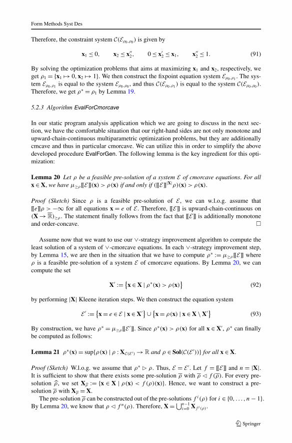
Form Methods Syst Des
Therefore, the constraint system C(Eρ0,ρ0) is given by
x1 ≤ 0, x2 ≤ x′′2, 0 ≤ x′2 ≤ x1, x′′2 ≤ 1. (91)
By solving the optimization problems that aims at maximizing x1 and x2, respectively, weget ρ1 = {x1 �→ 0,x2 �→ 1}. We then construct the fixpoint equation system Eρ0,ρ1 . The sys-tem Eρ0,ρ1 is equal to the system Eρ0,ρ0 , and thus C(Eρ0,ρ1) is equal to the system C(Eρ0,ρ0).Therefore, we get ρ∗ = ρ1 by Lemma 19.
5.2.3 Algorithm EvalForCmorcave
In our static program analysis application which we are going to discuss in the next sec-tion, we have the comfortable situation that our right-hand sides are not only monotone andupward-chain-continuous multiparametric optimization problems, but they are additionallycmcave and thus in particular cmorcave. We can utilize this in order to simplify the abovedeveloped procedure EvalForGen. The following lemma is the key ingredient for this opti-mization:
Lemma 20 Let ρ be a feasible pre-solution of a system E of cmorcave equations. For allx ∈ X, we have μ≥ρ[[E]](x) > ρ(x) if and only if ([[E]]|X|ρ)(x) > ρ(x).
Proof (Sketch) Since ρ is a feasible pre-solution of E , we can w.l.o.g. assume that[[e]]ρ > −∞ for all equations x = e of E . Therefore, [[E]] is upward-chain-continuous on(X →R)≥ρ . The statement finally follows from the fact that [[E]] is additionally monotoneand order-concave. �
Assume now that we want to use our ∨-strategy improvement algorithm to compute theleast solution of a system of ∨-cmorcave equations. In each ∨-strategy improvement step,by Lemma 15, we are then in the situation that we have to compute ρ∗ := μ≥ρ[[E]] whereρ is a feasible pre-solution of a system E of cmorcave equations. By Lemma 20, we cancompute the set
X′ := {x ∈ X | ρ∗(x) > ρ(x)}
(92)
by performing |X| Kleene iteration steps. We then construct the equation system
E ′ := {x = e ∈ E | x ∈ X′}∪ {x = ρ(x) | x ∈ X \X′} (93)
By construction, we have ρ∗ = μ≥ρ[[E ′]]. Since ρ∗(x) > ρ(x) for all x ∈ X′, ρ∗ can finallybe computed as follows:
Lemma 21 ρ∗(x)= sup{ρ(x) | ρ : XC(E ′) →R and ρ ∈ Sol(C(E ′))} for all x ∈ X.
Proof (Sketch) W.l.o.g. we assume that ρ∗ � ρ. Thus, E = E ′. Let f = [[E]] and n = |X|.It is sufficient to show that there exists some pre-solution ρ with ρ � f (ρ). For every pre-solution ρ, we set Xρ := {x ∈ X | ρ(x) < f (ρ)(x)}. Hence, we want to construct a pre-solution ρ with Xρ = X.
The pre-solution ρ can be constructed out of the pre-solutions f i(ρ) for i ∈ {0, . . . , n− 1}.By Lemma 20, we know that ρ � f n(ρ). Therefore, X =⋃n−1
i=0 Xf i (ρ).
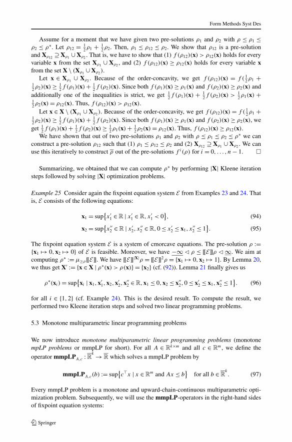
Form Methods Syst Des
Assume for a moment that we have given two pre-solutions ρ1 and ρ2 with ρ ≤ ρ1 ≤ρ2 ≤ ρ∗. Let ρ12 = 1
2ρ1 + 12 ρ2. Then, ρ1 ≤ ρ12 ≤ ρ2. We show that ρ12 is a pre-solution
and Xρ12 ⊇ Xρ1 ∪Xρ2 . That is, we have to show that (1) f (ρ12)(x) > ρ12(x) holds for everyvariable x from the set Xρ1 ∪ Xρ2 , and (2) f (ρ12)(x) ≥ ρ12(x) holds for every variable xfrom the set X \ (Xρ1 ∪Xρ2).
Let x ∈ Xρ1 ∪ Xρ2 . Because of the order-concavity, we get f (ρ12)(x) = f ( 12 ρ1 +
12ρ2)(x)≥ 1
2 f (ρ1)(x)+ 12 f (ρ2)(x). Since both f (ρ1)(x)≥ ρ1(x) and f (ρ2)(x)≥ ρ2(x) and
additionally one of the inequalities is strict, we get 12f (ρ1)(x) + 1
2f (ρ2)(x) > 12 ρ1(x) +
12ρ2(x)= ρ12(x). Thus, f (ρ12)(x) > ρ12(x).
Let x ∈ X \ (Xρ1 ∪ Xρ2). Because of the order-concavity, we get f (ρ12)(x) = f ( 12 ρ1 +
12ρ2)(x)≥ 1
2 f (ρ1)(x)+ 12f (ρ2)(x). Since both f (ρ1)(x)≥ ρ1(x) and f (ρ2)(x)≥ ρ2(x), we
get 12 f (ρ1)(x)+ 1
2 f (ρ2)(x)≥ 12 ρ1(x)+ 1
2ρ2(x)= ρ12(x). Thus, f (ρ12)(x)≥ ρ12(x).We have shown that out of two pre-solutions ρ1 and ρ2 with ρ ≤ ρ1 ≤ ρ2 ≤ ρ∗ we can
construct a pre-solution ρ12 such that (1) ρ1 ≤ ρ12 ≤ ρ2 and (2) Xρ12 ⊇ Xρ1 ∪ Xρ2 . We canuse this iteratively to construct ρ out of the pre-solutions f i(ρ) for i = 0, . . . , n− 1. �
Summarizing, we obtained that we can compute ρ∗ by performing |X| Kleene iterationsteps followed by solving |X| optimization problems.
Example 25 Consider again the fixpoint equation system E from Examples 23 and 24. Thatis, E consists of the following equations:
x1 = sup{x ′
1 ∈R | x ′1 ∈R, x ′
1 < 0}, (94)
x2 = sup{x ′′
2 ∈R | x ′2, x
′′2 ∈R,0 ≤ x ′
2 ≤ x1, x′′2 ≤ 1
}. (95)
The fixpoint equation system E is a system of cmorcave equations. The pre-solution ρ :={x1 �→ 0,x2 �→ 0} of E is feasible. Moreover, we have −∞ � ρ ≤ [[E]]ρ �∞. We aim atcomputing ρ∗ := μ≥ρ[[E]]. We have [[E]]|X|ρ = [[E]]2ρ = {x1 �→ 0,x2 �→ 1}. By Lemma 20,we thus get X′ := {x ∈ X | ρ∗(x) > ρ(x)} = {x2} (cf. (92)). Lemma 21 finally gives us
ρ∗(xi )= sup{xi | x1,x′1,x2,x′2,x′′2 ∈R,x1 ≤ 0,x2 ≤ x′′2,0 ≤ x′2 ≤ x1,x′′2 ≤ 1
}. (96)
for all i ∈ {1,2} (cf. Example 24). This is the desired result. To compute the result, weperformed two Kleene iteration steps and solved two linear programming problems.
5.3 Monotone multiparametric linear programming problems
We now introduce monotone multiparametric linear programming problems (monotonempLP problems or mmpLP for short). For all A ∈ R
k×m and all c ∈ Rm, we define the
operator mmpLPA,c :Rk →R which solves a mmpLP problem by
mmpLPA,c(b) := sup{c�x | x ∈R
m and Ax ≤ b}
for all b ∈Rk. (97)
Every mmpLP problem is a monotone and upward-chain-continuous multiparametric opti-mization problem. Subsequently, we will use the mmpLP-operators in the right-hand sidesof fixpoint equation systems:
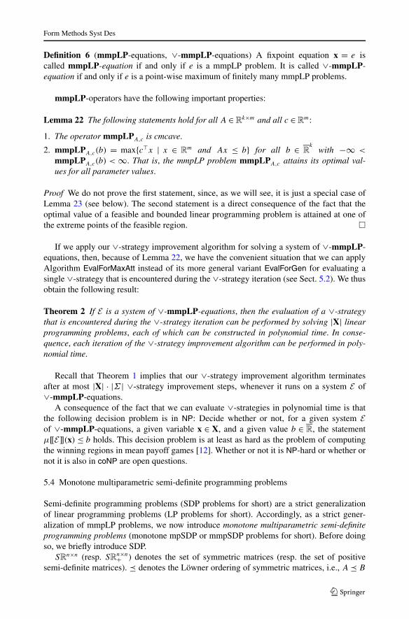
Form Methods Syst Des
Definition 6 (mmpLP-equations, ∨-mmpLP-equations) A fixpoint equation x = e iscalled mmpLP-equation if and only if e is a mmpLP problem. It is called ∨-mmpLP-equation if and only if e is a point-wise maximum of finitely many mmpLP problems.
mmpLP-operators have the following important properties:
Lemma 22 The following statements hold for all A ∈Rk×m and all c ∈R
m:
1. The operator mmpLPA,c is cmcave.
2. mmpLPA,c(b) = max{c�x | x ∈ Rm and Ax ≤ b} for all b ∈ R
kwith −∞ <
mmpLPA,c(b) < ∞. That is, the mmpLP problem mmpLPA,c attains its optimal val-ues for all parameter values.
Proof We do not prove the first statement, since, as we will see, it is just a special case ofLemma 23 (see below). The second statement is a direct consequence of the fact that theoptimal value of a feasible and bounded linear programming problem is attained at one ofthe extreme points of the feasible region. �
If we apply our ∨-strategy improvement algorithm for solving a system of ∨-mmpLP-equations, then, because of Lemma 22, we have the convenient situation that we can applyAlgorithm EvalForMaxAtt instead of its more general variant EvalForGen for evaluating asingle ∨-strategy that is encountered during the ∨-strategy iteration (see Sect. 5.2). We thusobtain the following result:
Theorem 2 If E is a system of ∨-mmpLP-equations, then the evaluation of a ∨-strategythat is encountered during the ∨-strategy iteration can be performed by solving |X| linearprogramming problems, each of which can be constructed in polynomial time. In conse-quence, each iteration of the ∨-strategy improvement algorithm can be performed in poly-nomial time.
Recall that Theorem 1 implies that our ∨-strategy improvement algorithm terminatesafter at most |X| · |Σ | ∨-strategy improvement steps, whenever it runs on a system E of∨-mmpLP-equations.
A consequence of the fact that we can evaluate ∨-strategies in polynomial time is thatthe following decision problem is in NP: Decide whether or not, for a given system Eof ∨-mmpLP-equations, a given variable x ∈ X, and a given value b ∈ R, the statementμ[[E]](x) ≤ b holds. This decision problem is at least as hard as the problem of computingthe winning regions in mean payoff games [12]. Whether or not it is NP-hard or whether ornot it is also in coNP are open questions.
5.4 Monotone multiparametric semi-definite programming problems
Semi-definite programming problems (SDP problems for short) are a strict generalizationof linear programming problems (LP problems for short). Accordingly, as a strict gener-alization of mmpLP problems, we now introduce monotone multiparametric semi-definiteprogramming problems (monotone mpSDP or mmpSDP problems for short). Before doingso, we briefly introduce SDP.
SRn×n (resp. SRn×n+ ) denotes the set of symmetric matrices (resp. the set of positive
semi-definite matrices). � denotes the Löwner ordering of symmetric matrices, i.e., A� B
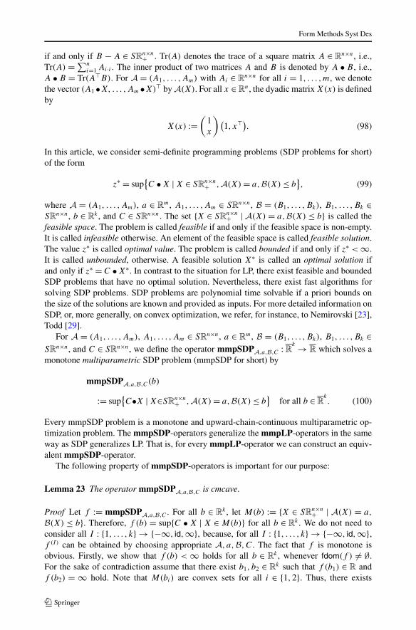
Form Methods Syst Des
if and only if B − A ∈ SRn×n+ . Tr(A) denotes the trace of a square matrix A ∈ R
n×n, i.e.,Tr(A) =∑n
i=1 Ai·i . The inner product of two matrices A and B is denoted by A • B , i.e.,A • B = Tr(A�B). For A = (A1, . . . ,Am) with Ai ∈ R
n×n for all i = 1, . . . ,m, we denotethe vector (A1 •X, . . . ,Am •X)� by A(X). For all x ∈R
n, the dyadic matrix X(x) is definedby
X(x) :=(
1x
)(1, x�). (98)
In this article, we consider semi-definite programming problems (SDP problems for short)of the form
z∗ = sup{C •X |X ∈ SRn×n
+ ,A(X)= a,B(X)≤ b}, (99)
where A = (A1, . . . ,Am), a ∈ Rm, A1, . . . ,Am ∈ SRn×n, B = (B1, . . . ,Bk), B1, . . . ,Bk ∈
SRn×n, b ∈ Rk , and C ∈ SRn×n. The set {X ∈ SRn×n
+ | A(X) = a,B(X) ≤ b} is called thefeasible space. The problem is called feasible if and only if the feasible space is non-empty.It is called infeasible otherwise. An element of the feasible space is called feasible solution.The value z∗ is called optimal value. The problem is called bounded if and only if z∗ <∞.It is called unbounded, otherwise. A feasible solution X∗ is called an optimal solution ifand only if z∗ = C •X∗. In contrast to the situation for LP, there exist feasible and boundedSDP problems that have no optimal solution. Nevertheless, there exist fast algorithms forsolving SDP problems. SDP problems are polynomial time solvable if a priori bounds onthe size of the solutions are known and provided as inputs. For more detailed information onSDP, or, more generally, on convex optimization, we refer, for instance, to Nemirovski [23],Todd [29].
For A = (A1, . . . ,Am), A1, . . . ,Am ∈ SRn×n, a ∈ Rm, B = (B1, . . . ,Bk), B1, . . . ,Bk ∈
SRn×n, and C ∈ SRn×n, we define the operator mmpSDPA,a,B,C : Rk → R which solves amonotone multiparametric SDP problem (mmpSDP for short) by
mmpSDPA,a,B,C(b)
:= sup{C•X |X∈SRn×n
+ ,A(X)= a,B(X)≤ b}
for all b ∈Rk. (100)
Every mmpSDP problem is a monotone and upward-chain-continuous multiparametric op-timization problem. The mmpSDP-operators generalize the mmpLP-operators in the sameway as SDP generalizes LP. That is, for every mmpLP-operator we can construct an equiv-alent mmpSDP-operator.
The following property of mmpSDP-operators is important for our purpose:
Lemma 23 The operator mmpSDPA,a,B,C is cmcave.
Proof Let f := mmpSDPA,a,B,C . For all b ∈ Rk , let M(b) := {X ∈ SRn×n
+ | A(X) = a,
B(X) ≤ b}. Therefore, f (b) = sup{C • X | X ∈ M(b)} for all b ∈ Rk . We do not need to
consider all I : {1, . . . , k} → {−∞, id,∞}, because, for all I : {1, . . . , k} → {−∞, id,∞},f (I) can be obtained by choosing appropriate A, a,B,C. The fact that f is monotone isobvious. Firstly, we show that f (b) < ∞ holds for all b ∈ R
k , whenever fdom(f ) �= ∅.For the sake of contradiction assume that there exist b1, b2 ∈ R
k such that f (b1) ∈ R andf (b2) = ∞ hold. Note that M(bi) are convex sets for all i ∈ {1,2}. Thus, there exists
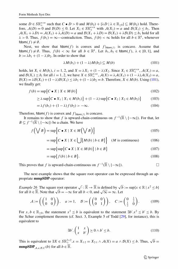
Form Methods Syst Des
some D ∈ SRn×n+ such that C •D > 0 and M(b2)+ {λD | λ ∈ R≥0} ⊆ M(b2) hold. There-
fore, A(D) = 0 and B(D) ≤ 0. Let X1 ∈ SRn×n+ with A(X1) = a and B(X1) ≤ b1. Then
A(X1 + λD)=A(X1)+ λA(D)= a and B(X1 + λD)= B(X1)+ λB(D)≤ b1 hold for allλ > 0. Thus, f (b1) =∞—contradiction. Thus, f (b) < ∞ holds for all b ∈ R
k , wheneverfdom(f ) �= ∅.
Next, we show that fdom(f ) is convex and f |fdom(f ) is concave. Assume thatfdom(f ) �= ∅. Thus, f (b) < ∞ for all b ∈ R
k . Let b1, b2 ∈ fdom(f ), λ ∈ [0,1], andb := λb1 + (1− λ)b2. In order to show that
λM(b1)+ (1− λ)M(b2)⊆M(b) (101)
holds, let Xi ∈M(bi), i = 1,2, and X = λX1 + (1 − λ)X2. Since Xi ∈ SRn×n+ , A(Xi)= a,
and B(Xi)≤ bi for all i = 1,2, we have X ∈ SRn×n+ , A(X)= λA(X1)+ (1− λ)A(X2)= a,
B(X)= λB(X1)+ (1−λ)B(X1)≤ λb1 + (1−λ)b2 = b. Therefore, X ∈M(b). Using (101),we finally get:
f (b)= sup{C •X |X ∈M(b)
}(102)
≥ λ sup{C •X1 |X1 ∈M(b1)
}+ (1− λ) sup{C •X2 |X2 ∈M(b2)
}(103)
= λf (b1)+ (1− λ)f (b2) >−∞. (104)
Therefore, fdom(f ) is convex and f |fdom(f ) is concave.It remains to show that f is upward-chain-continuous on f −1(R \ {−∞}). For that, let
B ⊆ f −1(R \ {−∞}) be a chain. We have
f(∨
B)= sup
{C •X |X ∈M
(∨B)}
(105)
= sup{C •X |X ∈
⋃{M(b) | b ∈ B
}}(M is continuous) (106)
= sup{sup{C •X |X ∈M(b)
} | b ∈ B}
(107)
= sup{f (b) | b ∈ B
}. (108)
This proves that f is upward-chain-continuous on f −1(R \ {−∞}). �
The next example shows that the square root operator can be expressed through an ap-propriate mmpSDP-operator:
Example 26 The square root operator√· :R→R is defined by
√b := sup{x ∈R | x2 ≤ b}
for all b ∈R. Note that√
b =−∞ for all b < 0, and√∞=∞. Let
A :=((
1 00 0
)), a := 1, B :=
((0 00 1
)), C :=
(0 1
212 0
). (109)
For x, b ∈ R≥0, the statement x2 ≤ b is equivalent to the statement ∃b′.x2 ≤ b′ ≤ b. Bythe Schur complement theorem (cf. Sect. 3, Example 5 of Todd [29], for instance), this isequivalent to
∃b′.(
1 x
x b′
)� 0∧ b′ ≤ b. (110)
This is equivalent to ∃X ∈ SR2×2+ .x = X1·2 = X2·1 ∧ A(X) = a ∧ B(X) ≤ b. Thus,
√b =
mmpSDPA,a,B,C(b) for all b ∈R.
Form Methods Syst Des
Definition 7 (mmpSDP-equations, ∨-mmpSDP-equations) A fixpoint equation x = e iscalled mmpSDP-equation if and only if e is a mmpSDP problem. It is called ∨-mmpSDP-equation if and only if e is a point-wise maximum of finitely many mmpSDP problems.
If E is a system of ∨-mmpSDP-equations, then, because of Lemma 23, we have the con-venient situation that we can apply Algorithm EvalForCmorcave instead of its more generalvariant EvalForGen (see Sect. 5.2) to evaluate the ∨-strategies that are encountered duringthe ∨-strategy iteration. This case is in particular interesting for the static program analysisapplication we are going to describe in Sect. 6.
Theorem 3 If E is a system of ∨-mmpSDP-equations, then the evaluation of a ∨-strategythat is encountered during the ∨-strategy iteration can be performed by performing |X|Kleene iteration steps and subsequently solving |X| SDP problems, each of which can beconstructed in polynomial time.
Recall that Theorem 1 implies that our ∨-strategy improvement algorithm terminatesafter at most |X| · |Σ | ∨-strategy improvement steps, whenever it runs on a system E of∨-mmpSDP-equations.
In order to obtain a good implementation of the proposed algorithm, a lot of non-trivialalgorithmic engineering is necessary. A clever implementation would try to reduce the num-ber of convex optimization problems and their sizes, for instance, by taking dependenciesinto account. Although these kind of optimizations are likely to be important in practice,a deeper study of such optimizations are out of the scope of this article and left for futurework.
6 Quadratic templates and relaxed abstract semantics
In this section, we apply our ∨-strategy improvement algorithm to a static program analysisproblem. For that, we first introduce a simple programming model as well as its collectingand its abstract semantics. We then relax the abstract semantics along the same lines asAdjé et al. [1] using Shor’s semi-definite relaxation schema. Finally, we use our algorithmto compute the relaxation of the abstract semantics.
6.1 A simple programming model and its collecting semantics
In our programming model, we consider statements of the following two forms:
1. x :=Ax + b, where A ∈Rn×n, and b ∈R
n (affine assignments)2. x�Ax + 2b�x ≤ c, where A ∈ SRn×n, b ∈R
n, and c ∈R (quadratic guards)
Here, x ∈ Rn denotes the vector of all program variables. We denote the set of statements
by Stmt. The collecting semantics [[s]] : 2Rn → 2R
nof a statement s ∈ Stmt is defined by:
[[x :=Ax + b]]X := {Ax + b | x ∈X} for all X ⊆Rn, (111)[[
x�Ax + 2b�x ≤ c]]X := {x ∈X | x�Ax + 2b�x ≤ c
}for all X ⊆R
n. (112)
A program G is a triple (N,E, st, I ), where N is a finite set of control-flow points, E ⊆N ×Stmt×N is a finite set of control-flow edges, st ∈N is the start control-flow point, and
Form Methods Syst Des
I ⊆Rn is a set of initial values. The collecting semantics V of a program G= (N,E, st, I )
is then the least solution of the following constraint system:
V[st] ⊇ I, V[v] ⊇ [[s]](V[u]) for all (u, s, v) ∈E. (113)
Here, the variables V[v], v ∈ N take values from 2Rn. The components of the collecting
semantics V are denoted by V [v] for all v ∈N .
6.2 Quadratic templates and abstract semantics
Along the lines of Adjé et al. [1], we define quadratic templates (in [1], templates are calledzones) as follows: A set P of functions p : Rn → R is a quadratic template if and only ifevery p ∈ P can be written as
p(x)= x�Apx + 2b�p x for all x ∈Rn, (114)
where Ap ∈ SRn×n and bp ∈ Rn for all p ∈ P . In the remainder of this article, we assume
that P = {p1, . . . , pm} is a finite quadratic template. Moreover, we assume w.l.o.g. that pi �=0 for all i = 1, . . . ,m. The abstraction α : 2R
n → P → R and the concretization γ : (P →R)→ 2R
nare defined as follows:
γ (v) := {x ∈Rn | ∀p ∈ P.p(x)≤ v(p)
}for all v : P →R, (115)
α(X) :=∧{
v : P →R | γ (v)⊇X}
for all X ⊆Rn. (116)
As shown by Adjé et al. [1], α and γ form a Galois-connection. The elements fromγ (P →R) and the elements from α(2R
n) are called closed. α(γ (v)) is called the closure of
v : P →R. Accordingly, γ (α(X)) is called the closure of X ⊆Rn.
As usual, the abstract semantics [[s]] : (P → R) → P → R of a statement s is definedby [[s]] := α ◦ [[s]] ◦ γ . The abstract semantics V of a program G = (N,E, st, I ) is thenthe least solution of the following constraint system:
V[st] ≥ α(I), V[v] ≥ [[s]](V[u]) for all (u, s, v) ∈E. (117)
Here, the variables V[v], v ∈ N take values in P → R. The components of the abstractsemantics V are denoted by V [v] for all v ∈N .
6.3 Relaxed abstract semantics
The problem of deciding, whether or not, for a given quadratic template P , a given v :P →Q, a given p ∈ P , and a given q ∈Q, α(γ (v))(p)≤ q holds, is NP-hard (cf. [1]) andthus intractable. Therefore, we use the relaxed abstract semantics V R introduced by Adjéet al. [1]. It is based on Shor’s semi-definite relaxation schema. In order to fit it into ourframework, we have to switch to the semi-definite dual. This is not a disadvantage. It isactually an advantage, since we potentially gain precision through this step, because of weakduality.
Definition 8 ([[x :=Ax + b]]R) We define the relaxed abstract semantics
[[x :=Ax + b]]R : (P →R)→ P →R (118)
Form Methods Syst Des
of an affine assignment x :=Ax + b by
[[x :=Ax + b]]Rv(p) := sup{A(p)•X ∣∣ ∀p′ ∈ P.Ap′ •X ≤ v
(p′),X � 0,X1·1 = 1
}(119)
for all v : P →R and all p ∈ P , where, for all p′ ∈ P ,
A(p) :=A�ApA, b(p) :=A�Apb+A�bp, c(p) := b�Apb+ 2b�p b,
A(p) :=(
c(p) b�(p)
b(p) A(p)
), Ap′ :=
(0 b�
p′bp′ Ap′
).
(120)
Definition 9 ([[x�Ax + 2b�x ≤ c]]R) We define the relaxed abstract semantics
[[x�Ax + 2b�x ≤ c
]]R : (P →R)→ P →R (121)
of a quadratic guard x�Ax + 2b�x ≤ c by
[[x�Ax + 2b�x ≤ c
]]Rv(p)
:= sup{Ap•X | ∀p′ ∈ P.Ap′ •X ≤ v
(p′), A•X ≤ 0,X � 0,X1·1 = 1
}(122)
for all v : P →R and all p ∈ P , where, for all p′ ∈ P ,
A :=(−c b�
b A
), Ap′ :=
(0 b�
p′bp′ Ap′
). (123)
Remark 2 A relaxation of the closure operator α ◦ γ = [[x := x]] is given by [[x := x]]R.As we will see below, we have α ◦ γ = [[x := x]] ≤ [[x := x]]R.
The relaxed abstract semantics [[·]]R is the semi-definite dual of the one used by Adjé etal. [1]. By weak-duality, it is at least as precise as the one used by Adjé et al. [1].
We have to show that the relaxed abstract semantics is indeed a relaxation of the ab-stract semantics. In order to utilize the results from the previous sections, we moreover haveto make sure that the relaxed abstract semantics of a statement is expressible through ammpSDP-operator.
Lemma 24 The following statements hold for every statement s ∈ Stmt:
1. [[s]] ≤ [[s]]R. That is, the relaxed abstract semantics correctly over-approximates theabstracts semantics.
2. For every i ∈ {1, . . . ,m}, there exist A, a,B,C such that
[[s]]Rv(pi)= mmpSDPA,a,B,C
(v(p1), . . . , v(pm)
)(124)
for all v : P →R. From s and P , the values A, a, B, and C can be computed in polyno-mial time.
Proof Since the second statement is obvious, we only prove the first one. We only considerthe case that s is an affine assignment x :=Ax + b. The case that s is a quadratic guard canbe treated along the same lines. Let v : P →R, p ∈ P , and v′ := [[x :=Ax + b]]v. Then,
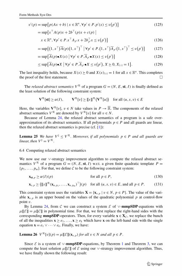
Form Methods Syst Des
v′(p)= sup{p(Ax + b) | x ∈R
n,∀p′ ∈ P.p′(x)≤ v(p′)} (125)
= sup{x�A(p)x + 2b�(p)x + c(p)
∣∣x ∈R
n,∀p′ ∈ P.x�Ap′x + 2b�p′x ≤ v(p′)} (126)
= sup{(
1, x�)A(p)(1, x�)� ∣∣ ∀p′ ∈ P.
(1, x�)Ap′
(1, x�)� ≤ v
(p′)} (127)
= sup{A(p)•X(x)
∣∣ ∀p′ ∈ P.Ap′ •X(x)≤ v(p′)} (128)
≤ sup{A(p)•X ∣∣ ∀p′ ∈ P.Ap′ •X ≤ v
(p′),X � 0,X1·1 = 1
}. (129)
The last inequality holds, because X(x)� 0 and X(x)1·1 = 1 for all x ∈Rn. This completes
the proof of the first statement. �
The relaxed abstract semantics V R of a program G= (N,E, st, I ) is finally defined asthe least solution of the following constraint system:
VR[st] ≥ α(I), VR[v] ≥ [[s]]R(VR[u]) for all (u, s, v) ∈E
Here, the variables VR[v], v ∈ N take values in P → R. The components of the relaxedabstract semantics V R are denoted by V R[v] for all v ∈N .
Because of Lemma 24, the relaxed abstract semantics of a program is a safe over-approximation of its abstract semantics. If all polynomials p ∈ P and all guards are linear,then the relaxed abstract semantics is precise (cf. [1]):
Lemma 25 We have V ≤ V R. Moreover, if all polynomials p ∈ P and all guards arelinear, then V = V R.
6.4 Computing relaxed abstract semantics
We now use our ∨-strategy improvement algorithm to compute the relaxed abstract se-mantics V R of a program G = (N,E, st, I ) w.r.t. a given finite quadratic template P ={p1, . . . , pm}. For that, we define C to be the following constraint system:
xst,p ≥ α(I)(p) for all p ∈ P, (130)
xv,p ≥([[s]]R(xu,p1 , . . . ,xu,pm)�
)(p) for all (u, s, v) ∈E, and all p ∈ P. (131)
This constraint system uses the variables X = {xv,p | v ∈ N,p ∈ P }. The value of the vari-able xv,p is an upper bound on the values of the quadratic polynomial p at control-flowpoint v.
By Lemma 24, from C we can construct a system E of ∨-mmpSDP-equations withμ[[E]] = μ[[C]] in polynomial time. For that, we first replace the right-hand sides with thecorresponding mmpSDP-operators. Then, for every variable x ∈ XC , we replace the bunchof all the inequalities x ≥ e1, . . . ,x ≥ ek which have x on the left-hand side with the singleequation x = e1 ∨ · · · ∨ ek . Finally, we have:
Lemma 26 V R[v](p)= μ[[E]](xv,p) for all v ∈N and all p ∈ P .
Since E is a system of ∨-mmpSDP-equations, by Theorem 1 and Theorem 3, we cancompute the least solution μ[[E]] of E using our ∨-strategy improvement algorithm. Thus,we have finally shown the following result:
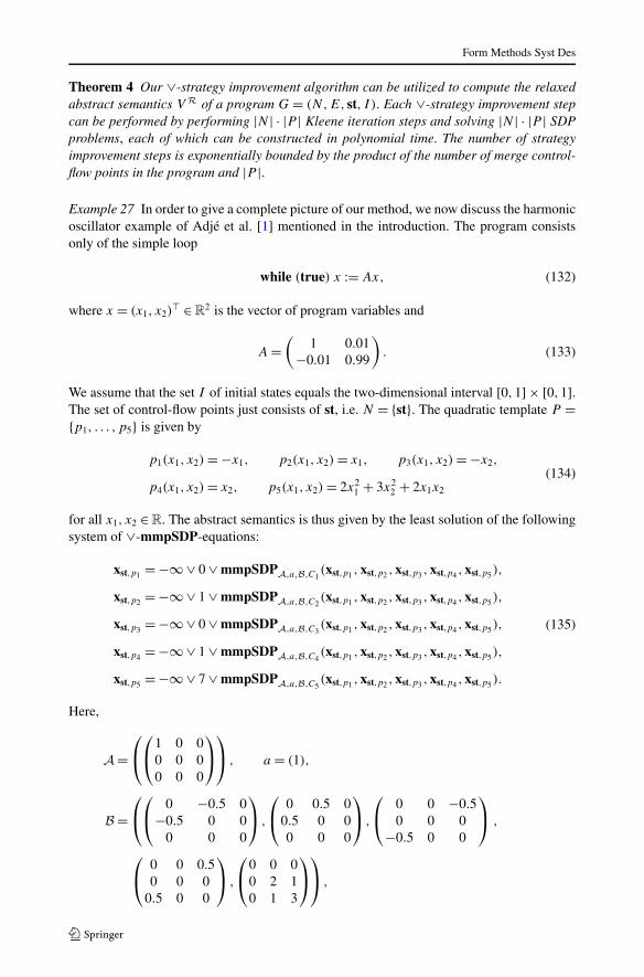
Form Methods Syst Des
Theorem 4 Our ∨-strategy improvement algorithm can be utilized to compute the relaxedabstract semantics V R of a program G= (N,E, st, I ). Each ∨-strategy improvement stepcan be performed by performing |N | · |P | Kleene iteration steps and solving |N | · |P | SDPproblems, each of which can be constructed in polynomial time. The number of strategyimprovement steps is exponentially bounded by the product of the number of merge control-flow points in the program and |P |.
Example 27 In order to give a complete picture of our method, we now discuss the harmonicoscillator example of Adjé et al. [1] mentioned in the introduction. The program consistsonly of the simple loop
while (true) x :=Ax, (132)
where x = (x1, x2)� ∈R
2 is the vector of program variables and
A=(
1 0.01−0.01 0.99
). (133)
We assume that the set I of initial states equals the two-dimensional interval [0,1] × [0,1].The set of control-flow points just consists of st, i.e. N = {st}. The quadratic template P ={p1, . . . , p5} is given by
p1(x1, x2)=−x1, p2(x1, x2)= x1, p3(x1, x2)=−x2,
p4(x1, x2)= x2, p5(x1, x2)= 2x21 + 3x2
2 + 2x1x2
(134)
for all x1, x2 ∈R. The abstract semantics is thus given by the least solution of the followingsystem of ∨-mmpSDP-equations:
xst,p1 =−∞∨ 0∨mmpSDPA,a,B,C1(xst,p1 ,xst,p2 ,xst,p3 ,xst,p4 ,xst,p5),
xst,p2 =−∞∨ 1∨mmpSDPA,a,B,C2(xst,p1 ,xst,p2 ,xst,p3 ,xst,p4 ,xst,p5),
xst,p3 =−∞∨ 0∨mmpSDPA,a,B,C3(xst,p1 ,xst,p2 ,xst,p3 ,xst,p4 ,xst,p5),
xst,p4 =−∞∨ 1∨mmpSDPA,a,B,C4(xst,p1 ,xst,p2 ,xst,p3 ,xst,p4 ,xst,p5),
xst,p5 =−∞∨ 7∨mmpSDPA,a,B,C5(xst,p1 ,xst,p2 ,xst,p3 ,xst,p4 ,xst,p5).
(135)
Here,
A=⎛⎝⎛⎝1 0 0
0 0 00 0 0
⎞⎠⎞⎠ , a = (1),
B =⎛⎝⎛⎝ 0 −0.5 0−0.5 0 0
0 0 0
⎞⎠ ,
⎛⎝ 0 0.5 0
0.5 0 00 0 0
⎞⎠ ,
⎛⎝ 0 0 −0.5
0 0 0−0.5 0 0
⎞⎠ ,
⎛⎝ 0 0 0.5
0 0 00.5 0 0
⎞⎠ ,
⎛⎝0 0 0
0 2 10 1 3
⎞⎠⎞⎠ ,
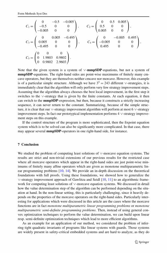
Form Methods Syst Des
C1 =⎛⎝ 0 −0.5 −0.005
−0.5 0 0−0.005 0 0
⎞⎠ , C2 =
⎛⎝ 0 0.5 0.005
0.5 0 00.005 0 0
⎞⎠ ,
C3 =⎛⎝ 0 0.005 −0.495
0.005 0 0−0.495 0 0
⎞⎠ , C4 =
⎛⎝ 0 −0.005 0.495−0.005 0 00.495 0 0
⎞⎠ ,
C5 =⎛⎝0 0 0
0 1.9803 0.98020 0.9802 2.9603
⎞⎠ .
Note that the given system is a system of ∨-mmpSDP-equations, but not a system ofmmpSDP-equations. The right-hand sides are point-wise maximums of finitely many cm-cave operators, but they are themselves neither cmcave nor morcave. However, this exampleis of a particular simple structure. Although we have 35 = 243 different ∨-strategies, it isimmediately clear that the algorithm will only perform very few strategy improvement steps.Assuming that the algorithm always chooses the best local improvement, in the first step itswitches to the ∨-strategy that is given by the finite constants. At each equation, it thencan switch to the mmpSDP-expression, but then, because it constructs a strictly increasingsequence, it can never return to the constant. Summarizing, because of the simple struc-ture, it is clear that our ∨-strategy improvement algorithm will perform at most 6 ∨-strategyimprovement steps. In fact our prototypical implementation performs 4 ∨-strategy improve-ment steps on this example.
If the control structure of the program is more sophisticated, then the fixpoint equationsystem which is to be solved can also be significantly more complicated. In that case, theremay appear several mmpSDP-operators in one right-hand side, for instance.
7 Conclusion
We studied the problem of computing least solutions of ∨-morcave equation systems. Theresults are strict and non-trivial extensions of our previous results for the restricted casewhere all morcave operators which appear in the right-hand sides are just point-wise min-imums of finitely many affine operators which are given as monotone multiparametric lin-ear programming problems [10, 14]. We provide an in-depth discussion on the theoreticalfoundations with full proofs. Using these foundations, we showed how to generalize the∨-strategy improvement approach of Gawlitza and Seidl [10, 11] to an algorithmic frame-work for computing least solutions of ∨-morcave equation systems. We discussed in detailhow the value determination step of the algorithm can be performed depending on the situ-ation at hand. In the non-linear setting, this is particularly challenging, since it heavily de-pends on the properties of the morcave operators on the right-hand sides. Particularly inter-esting for applications which were discussed in this article are the cases where the morcavefunctions are in fact monotone multiparametric linear programming problems or monotonemultiparametric semi-definite programming problems. Then, instead of using general con-vex optimization techniques to perform the value determination, we can build upon linearresp. semi-definite optimization techniques which lead to more efficient algorithms.
As an example for an application of our method, we considered the problem of infer-ring tight quadratic invariants of programs like linear systems with guards. Those systemsare widely present in safety-critical embedded systems and are hard to analyze, as they do
Form Methods Syst Des
not admit simple linear invariants. Our method can be used as a building block within ananalyzer for such systems. Roux and Garoche [24] actually use our methods within theiranalyzer for Lustre programs. In the conference article that appears in the proceedings ofthe Seventeenth International Static Analysis Symposium (SAS 2010) we report on experi-mental results that were obtained through our proof-of-concept implementation [13]. For amore detailed case study we refer to Roux and Garoche [24]. Besides the above-mentionedapplications, our method can also be used for proving program termination [20], where ithas to be adapted to compute greatest solutions instead of least solutions.
8 Future work
Concerning the static analysis application we studied in this article, it would be interestingto study the use of other convex relaxation schemes in order to deal with more sophisticatedprograms and abstractions; a problem already posed by Adjé et al. [1]. It also remains toinvestigate in how far our algorithms can be fruitfully applied to other applications—maybein other fields of computer science. Since our algorithmic framework solves quite generaland natural fixpoint problems, it has good chances to be also relevant in other areas. Naturalcandidates could be found in the context of quantitative synthesis. It might also be fruitfullyapplied to the analysis of non-linear hybrid systems. To the analysis of affine hybrid systemsrestricted versions of our method were already applied by Dang and Gawlitza [7, 8], afterthe min-strategy improvement approach of Costan et al. [4] was successfully applied to thisproblem [27].
Since this article focused on setting the theoretical foundations, giving elaborated proofs,and discussing relevant subclasses, many questions that are relevant in practice are left open.An example are all the challenges that are caused by numerical instabilities. In practice weare unfortunately not able to solve non-linear convex optimization problems precisely. Evenin the case of linear programming problems it can be impractical to solve them preciselyif the problem sizes are huge. Thus, our method naturally has to deal with numerical in-stabilities. This is an important issue, since, because of the presence of discontinuities inthe right-hand sides of the equation systems, small numerical errors can lead to signifi-cant errors. For instance, the decision to switch from one ∨-strategy to another allegedimproved ∨-strategy might be based on a numerical error and is thus a wrong decision.Hence, caused by small numerical errors, our algorithm might return a vastly wrong resultwhich might even be unsound. First steps to fight numerical problems are made by Roux andGaroche [24]. However, further investigations are necessary. Moreover, in order to obtain agood implementation of the proposed algorithm, a lot of non-trivial algorithmic engineeringis necessary. A clever implementation would try to reduce the number of convex optimiza-tion problems and their sizes, for instance, by taking dependencies into account. These kindof optimizations are likely to be important in practice. Their study is left for future work.
Acknowledgements The authors would like to thank the anonymous reviewers for their valuable com-ments and suggestions.
References
1. Adjé A, Gaubert S, Goubault E (2010) Coupling policy iteration with semi-definite relaxation to computeaccurate numerical invariants in static analysis. In: Gordon AD (ed) ESOP. Lecture notes in computerscience, vol 6012. Springer, Berlin, pp 23–42. ISBN 978-3-642-11956-9

Form Methods Syst Des
2. Alegre F, Feron E, Pande S (2009) Using ellipsoidal domains to analyze control systems software.arXiv:0909.1977
3. Caspi P, Pilaud D, Halbwachs N, Plaice J (1987) Lustre: a declarative language for programming syn-chronous systems. In: POPL. ACM, New York, pp 178–188. ISBN 0-89791-215-2
4. Costan A, Gaubert S, Goubault E, Martel M, Putot S (2005) A policy iteration algorithm for computingfixed points in static analysis of programs. In: Computer aided verification, 17th int conf (CAV). Lecturenotes in computer science, vol 3576. Springer, Berlin, pp 462–475
5. Cousot P, Cousot R (1976) Static determination of dynamic properties of programs. In: Second int sympon programming. Dunod, Paris, pp 106–130
6. Cousot P, Cousot R (1977) Abstract interpretation: a unified lattice model for static analysis of programsby construction or approximation of fixpoints. In: POPL, pp 238–252
7. Dang T, Gawlitza TM (2011) Template-based unbounded time verification of affine hybrid automata. In:Yang H (ed) APLAS. Lecture notes in computer science, vol 7078. Springer, Berlin, pp 34–49. ISBN978-3-642-25317-1
8. Dang T, Gawlitza TM (2011) Discretizing affine hybrid automata with uncertainty. In: Bultan T, HsiungP-A (eds) ATVA. Lecture notes in computer science, vol 6996. Springer, Berlin, pp 473–481. ISBN978-3-642-24371-4
9. Fearnley J (2010) Exponential lower bounds for policy iteration. In: Abramsky S, Gavoille C, KirchnerC, Meyer auf der Heide F, Spirakis PG (eds) ICALP (2). Lecture notes in computer science, vol 6199.Springer, Berlin, pp 551–562. ISBN 978-3-642-14161-4
10. Gawlitza T, Seidl H (2007) Precise relational invariants through strategy iteration. In: Duparc J, Hen-zinger TA (eds) CSL. Lecture notes in computer science, vol 4646. Springer, Berlin, pp 23–40. ISBN978-3-540-74914-1
11. Gawlitza T, Seidl H (2007) Precise fixpoint computation through strategy iteration. In: Nicola RD (ed)ESOP. Lecture notes in computer science, vol 4421. Springer, Berlin, pp 300–315. ISBN 978-3-540-71314-2
12. Gawlitza T, Seidl H (2008) Precise interval analysis vs. parity games. In: Cuéllar J, Maibaum TSE, SereK (eds) FM. Lecture notes in computer science, vol 5014. Springer, Berlin, pp 342–357. ISBN 978-3-540-68235-6
13. Gawlitza TM, Seidl H (2010) Computing relaxed abstract semantics w.r.t. quadratic zones precisely. In:Cousot R, Martel M (eds) SAS. Lecture notes in computer science, vol 6337. Springer, Berlin, pp 271–286. ISBN 978-3-642-15768-4
14. Gawlitza TM, Seidl H (2011) Solving systems of rational equations through strategy iteration. ACMTrans Program Lang Syst 33(3):11
15. Gawlitza TM, Seidl H, Adjé A, Gaubert S, Goubault É (2011) Abstract interpretation meets convexoptimization. In: WING-JSC
16. Girard A (2005) Reachability of uncertain linear systems using zonotopes. In: Morari M, Thiele L (eds)HSCC. Lecture notes in computer science, vol 3414. Springer, Berlin, pp 291–305. ISBN 3-540-25108-1
17. Halbwachs N (2005) A synchronous language at work: the story of lustre. In: MEMOCODE. IEEE Press,New York, pp 3–11
18. Halbwachs N, Lagnier F, Ratel C (1992) Programming and verifying real-time systems by means of thesynchronous data-flow language lustre. IEEE Trans Softw Eng 18(9):785–793
19. Larsen KG, Larsson F, Pettersson P, Yi W (1997) Efficient verification of real-time systems: compactdata structure and state-space reduction. In: IEEE real-time systems symposium. IEEE Comput Soc, LosAlamitos, pp 14–24
20. Massé D (2012) Proving termination by policy iteration. Electron Notes Theor Comput Sci 287:77–88.doi:10.1016/j.entcs.2012.09.008
21. Miné A (2001) A new numerical abstract domain based on difference-bound matrices. In: Danvy O,Filinski A (eds) PADO. Lecture notes in computer science, vol 2053. Springer, Berlin, pp 155–172.ISBN 3-540-42068-1
22. Miné A (2001) The octagon abstract domain. In: WCRE, p 31023. Nemirovski A (2005) Modern convex optimization. Department ISYE, Georgia Institute of Technology24. Roux P, Garoche P-L (2012) Policy iterations as traditional abstract domains25. Roux P, Jobredeaux R, Garoche P-L, Feron E (2012) A generic ellipsoid abstract domain for linear time
invariant systems. In: Dang T, Mitchell IM (eds) HSCC. ACM, New York, pp 105–114. ISBN 978-1-4503-1220-2
26. Sankaranarayanan S, Sipma HB, Manna Z (2005) Scalable analysis of linear systems using mathematicalprogramming. In: Cousot R (ed) VMCAI. Lecture notes in computer science, vol 3385. Springer, Berlin,pp 25–41. ISBN 3-540-24297-X
27. Sankaranarayanan S, Dang T, Ivancic F (2008) A policy iteration technique for time elapse over tem-plate polyhedra. In: Egerstedt M, Mishra B (eds) HSCC. Lecture notes in computer science, vol 4981.Springer, Berlin, pp 654–657. ISBN 978-3-540-78928-4

Form Methods Syst Des
28. Tarski A (1955) A lattice-theoretical fixpoint theorem and its applications. Pac J Math 5:285–30929. Todd MJ (2001) Semidefinite optimization. Acta Numer 10:515–56030. Yovine S (1996) Model checking timed automata. In: Rozenberg G, Vaandrager FW (eds) European
educational forum: school on embedded systems. Lecture notes in computer science, vol 1494. Springer,Berlin, pp 114–152. ISBN 3-540-65193-4


![T-76.4115 Iteration Demo Tikkaajat [PP] Iteration 18.10.2007.](https://static.fdocuments.net/doc/165x107/5a4d1b607f8b9ab0599ace21/t-764115-iteration-demo-tikkaajat-pp-iteration-18102007.jpg)