Numerical Integration(Quadrature)

Sachin ShanbhagDept. Scientific Computing

(based on material borrowed from Dennis Duke, Samir Al-Amer,David Kofke, Holistic Numerical Methods Institute)

Numerical Integration

Why do we need it?

• many integrals cannot be evaluated analytically• even if you can, you might need to check your answer• even if you can, numerical evaluation of the answer can be bothersome

Examples:

00

( 1)2

cosh 2 1

k

k

dx

x x k!

""

=

#=

+$%

!

e"x 2

dxa

b

#

Error function

An example of an integral that needs checking:

Possible Issues

the integrand is some sort of table of numbers• regularly spaced• irregularly spaced• contaminated with noise (experimental data)

the integrand is computable everywhere in the range of integration,but there may be• infinite range of integration• local discontinuities

considerations• time to compute the integral• estimate of the error due to

- truncation- round-off- noise in tabulated values

• In the differential limit, an integral is equivalent to a summationoperation:

• Approximate methods for determining integrals are mostly based onidea of area between integrand and axis.

Integral as Riemann sum

!

f (x)dxa

b

" = limn#$

f (xi)%xi= 0

i= n

& ' f (xi)%xi= 0

N(1

&

Let’s try a simple example

-0.0007670.001534102410-0.0015330.0030685129-0.0030650.0061362568-0.0061230.0122721287-0.0122220.024544646-0.0243430.049087325-0.0482840.098175164-0.0949600.19635083-0.1834650.39269942-0.3407590.78539821errordxintervalsn

Note that the error is decreasing by a factor 2, just like our discretization interval dx.

Question: Why is the error = I(exact) - I(calc) negative?

/2/2

0 0

cos sin 1xdx x!!

= ="

Analytically

Instead of having the top of the rectangle hit the left (or right) edge we could alsohave it hit the function at the midpoint of each interval:

!

f (x)dxa

b

" # f (xi + xi+1

2)$x

i= 0

N%1

&

Note that the lines at the top of therectangles can have any slopewhatsoever and we will always getthe same answer.

-0.0000000980.001534102410

-0.0000003920.0030685129

-0.0000015690.0061362568

-0.0000062750.0122721287

-0.0000251000.024544646

-0.0001004060.049087325

-0.0004017080.098175164

-0.0016081890.19635083

-0.0064545430.39269942

-0.0261721530.78539821

errordxintervalsn

now the error is falling by a factor 4 witheach halving of the interval dx.

Question: Why is the error smaller?

Question: Why is the error smaller?

Answer:

• One reason is that in the mid-point rule, the maximum distance over which we“extrapolate” our knowledge of f(x) is halved.

• Different integration schemes result from what we think the function is doingbetween evaluation points.

• Link between interpolation and numerical integration

Orientation

• Newton-Cotes MethodsUse intepolating polynomials. Trapezoid, Simpson’s 1/3 and 3/8 rules,Bode’s are special cases of 1st, 2nd, 3rd and 4th order polynomials areused, respectively

• Romberg Integration (Richardson Extrapolation)use knowledge of error estimates to build a recursive higher orderscheme

• Gauss QuadratureLike Newton-Cotes, but instead of a regular grid, choose a set that letsyou get higher order accuracy

• Monte Carlo IntegrationUse randomly selected grid points. Useful for higher dimensionalintegrals (d>4)

Newton-Cotes Methods

• In Newton-Cotes Methods, the function is approximated by a polynomialof order n

• To do this, we use ideas learnt from interpolation• Computing the integral of a polynomial is easy.

!

f (x)dx "a

b

# a0

+ a1x + ...+ anx

n( )dxa

b

#

!

f (x)dx "a

b

# a0(b $ a) + a

1

(b2 $ a2)

2+ ...+ an

(bn+1 $ an+1

)

n +1!

f (x) " a0

+ a1x + ...+ anx

n

we approximate the function f(x) in the interval [a,b] as:

interpolation

Trapezoid Method (First Order Polynomial are used)

Newton-Cotes Methods

!

f (x)dx "a

b

# a0

+ a1x( )dx

a

b

#

f(x)

ba ( )2

)()(

2

)()(

)()()(

)()()(

)(

)(

2

afbfab

x

ab

afbf

xab

afbfaaf

dxaxab

afbfafI

dxxfI

b

a

b

a

b

a

b

a

+!=

!

!+

"#

$%&

'

!

!!=

"#

$%&

'!

!

!+(

=

)

)

)()()(

)( axab

afbfaf !

!

!+

!

If the interval is divided into n segments(not necessarily equal)

a = x0 " x1 " x2 " ..." xn = b

f (x)dx #a

b

$1

2i= 0

n%1

& xi+1 % xi( ) f (xi+1) + f (xi)( )

!

Special Case (Equally spaced base points)

xi+1 " xi = h for all i

f (x)dx #a

b

$ h1

2f (x0) + f (xn )[ ] + f (xi)

i=1

n"1

%&

' (

)

* +

Multi-step Trapezoid Method

0.000000200.00153398102410

0.000000780.003067965129

0.000003140.006135922568

0.000012550.012271851287

0.000050200.02454369646

0.000200810.04908739325

0.000803320.09817477164

0.003214830.1963495483

0.012884200.3926990842

0.051940550.7853981621

errordxintervalsn /2/2

0 0

cos sin 1xdx x!!

= ="

Multi-step Trapezoid Method

Now the error is again decreasingby a factor 4, so like dx2.

In fact, it can be shown that:

!

Error "b # a

12h2maxx$[a,b ]

f ' '(x)

Simpson 1/3 RuleSecond Order Polynomial are used

Newton-Cotes Methods

!

f (x)dx "a

b

# a0

+ a1x + a

2x2( )dx

a

b

#

Simpson 3/8 RuleThird Order Polynomial are used,

!

f (x)dx "a

b

# a0

+ a1x + a

2x2 + a

3x3( )dx

a

b

#

f(x)

ba

h

f(x)

ba

h

h=(b-a)/2

h=(b-a)/3

Newton-Cotes Methods

wikipedia.org

These are called “closed” because we use function evaluations at the end-pointsof the interval. There are “open” formulae which don’t evalute f(a) and f(b), but wewon’t discuss them here.

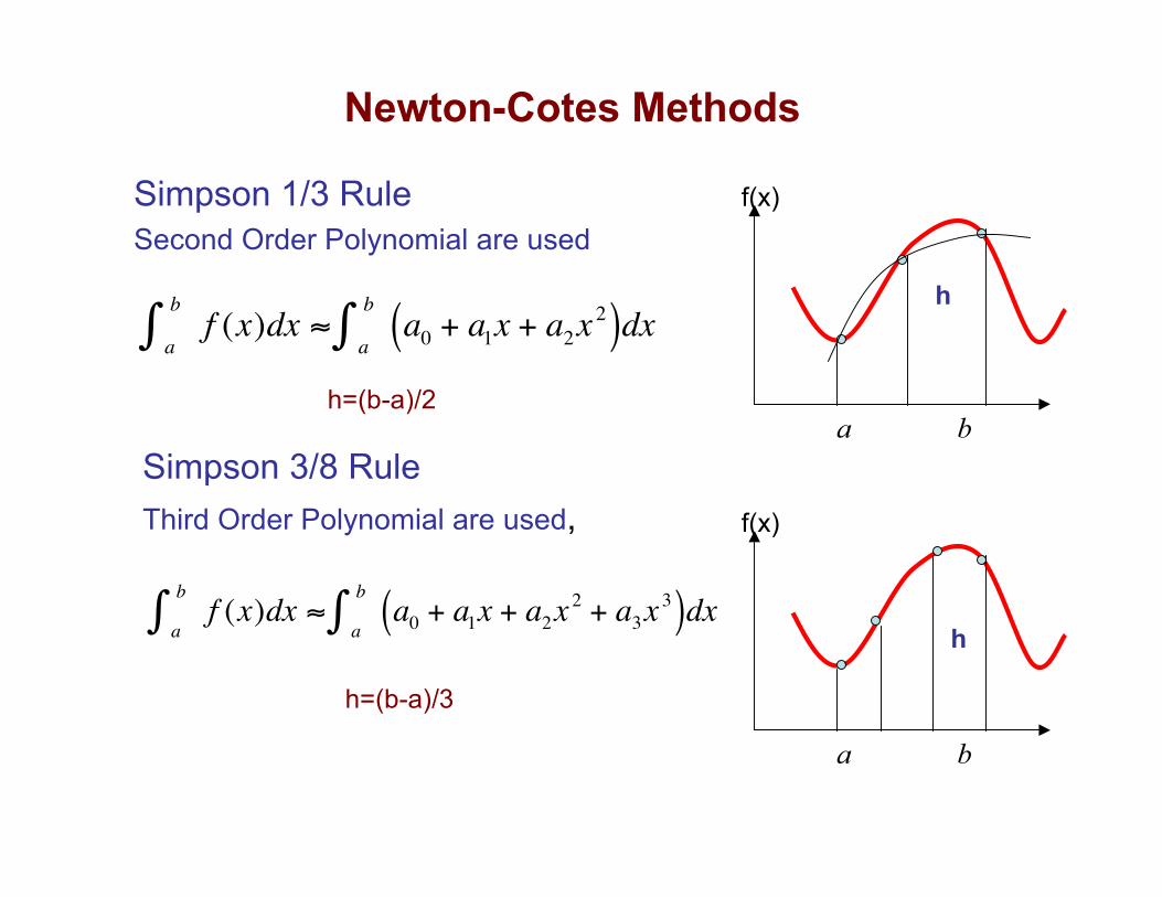
• Trapezoid formula with an interval h gives error of the order O(h2)

• Can we combine two Trapezoid estimates with intervals 2h and h to get abetter estimate?

• For a multistep trapezoidal rule, the error is:

• Think of as an approximate average value of f”(x) in [a,b]. Then,

Romberg Integration

!

Et =b " a( )

3

12n2

# # f $ i( )i=1

n

%

n

where ξi ∈ [ a+(i-1)h, a+ih ]

!

" " f # i( )i=1

n

$

n

!

Et"C

n2

! "#

$%&

'()*

+,-

.

(=30

8

892100140000

1400002000 dtt.

tlnx

Romberg IntegrationHow good is this approximation?

Consider

12.9110748

16.8110787

22.9110846

33.0110945

51.5111134

91.4111533

205112662

807118681

EtValuen

Vertical distance covered by arocket between 8 to 30seconds

Exact value x=11061 meters

The true error gets approximately quartered as the number ofsegments is doubled. This information is used to get a betterapproximation of the integral, and is the basis of RombergIntegration (or Richardson’s extrapolation).

Romberg Integration

2n

CEt! where C is an approximately constant

If Itrue = true value and In= approx. value of the integral

Itrue ≈ In + Et

Et(n) ≈ C/n2 ≈ Itrue - In Et(2n) ≈ C/4n2 ≈ Itrue - I2n

Therefore, eliminate C/n2 between these two equations

!

Itrue

" Itrue,est

= I2n

+I2n# I

n

3

Note: What we calculateis still an approximationfor Itrue

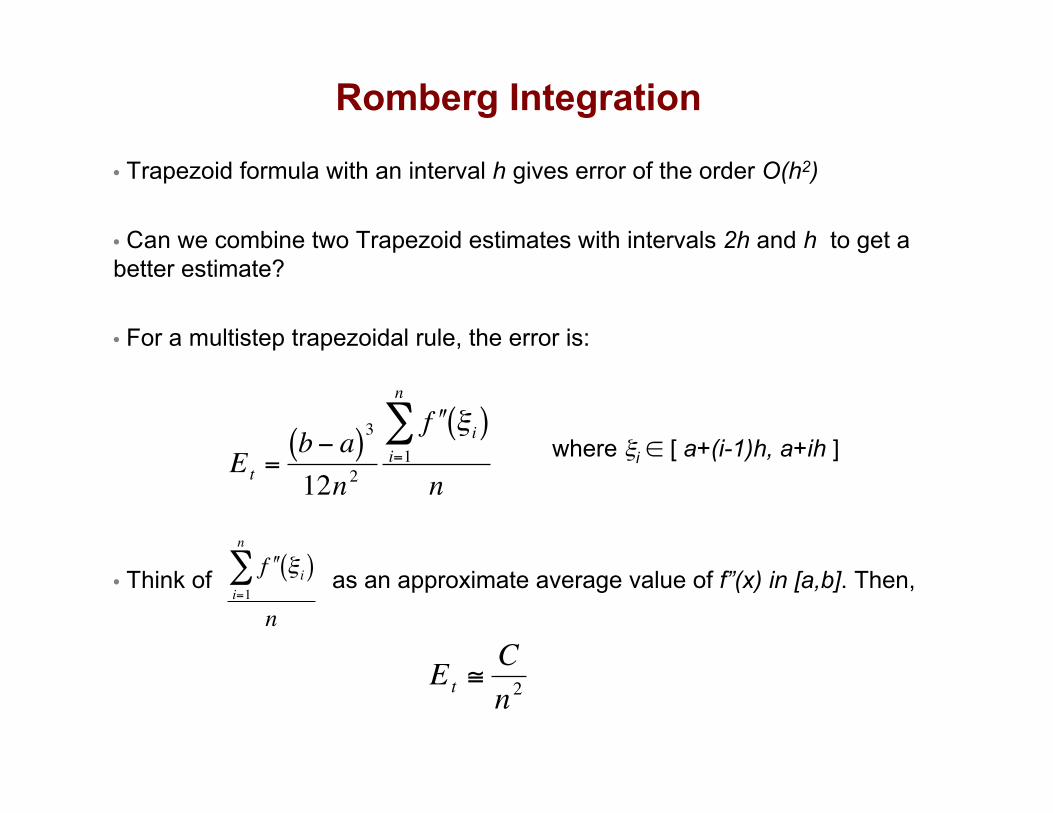
Example

The vertical distance covered by a rocket from 8 to 30 seconds is given by

! "#

$%&

'()*

+,-

.

(=30

8

892100140000

1400002000 dtt.

tlnx

1. Use Richardson’s rule to find thedistance covered (use table formultistep trapezoidal rule).

2. Find the true error, Et for part (1).

0.116512.9110748

0.152116.8110787

0.207022.9110846

0.298133.0110945

0.465551.5111134

0.826591.4111533

1.854205112662

7.296807118681

RelErrEtValuen

Multistep trapezoidal rule

Exact value=11061 meters

mI 112662=

mI 111134=

Using Richardson’s extrapolation formula for Trapezoidalrule, choosing n=2

Solution

!

Itrue

" I2n

+I2n# I

n

3

= 11062 m (Itrue,est)

Et = Iexact - Itrue,est = -1 m

10011061

1106211061!

"=#

t

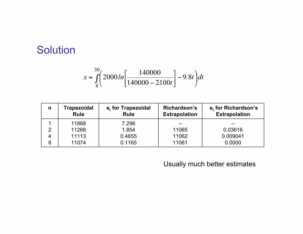
--0.03616

0.0090410.0000

--110651106211061

7.2961.8540.46550.1165

11868112661111311074

1248

et for Richardson’sExtrapolation

Richardson’sExtrapolation

et for TrapezoidalRule

TrapezoidalRule

n

Solution

! "#

$%&

'()*

+,-

.

(=30

8

892100140000

1400002000 dtt.

tlnx

Usually much better estimates

Romberg Integration: Successive Refinement

!

I2n

(k )=4kI2n

(k"1)" I

n

(k"1)

4k"1"1

,k # 2

• The index k represents the order of extrapolation.

• In(1) represents the values obtained from the regular Trapezoidalrule with n intervals.

• k=2 represents values obtained using the true estimate as O(h2).

• In(k) has an error of the order 1/n2k.

A general expression for Romberg integration can be written as

Romberg Integration: Successive Iteration

11868

1126

11113

11074

11065

11062

11061

11062

11061

11061

1-segment

2-segment

4-segment

8-segment

First Order(k=2)

Second Order(k=3)

Third Order(k=4)

For our particular example:

Questions from last class:

1. What is the error in Romberg integration?

!

Et"C1

n2

+C2

n4

+C3

n6...

!

Itrue

" Itrue,est

= I2n

+I2n# I

n

3

Over here identical toSimpson’s rule.

In fact this is how Numerical Recipes (Press et al.) implements the Simpson’s rule

This has an error of the order 1/n2k.

Successive iterations:

!

I2n

(k )=4kI2n

(k"1)" I

n

(k"1)

4k"1"1

,k # 2

O(1/n4)

Questions from last class:

2. Is Romberg better than Simpson’s?

This has an error of the order 1/n2k.

Successive iterations:

!

I2n

(k )=4kI2n

(k"1)" I

n

(k"1)

4k"1"1

,k # 2

So usually, yes!

To evaluate an integral to the same degree of accuracy, you need fewerfunction evaluations with Romberg.

!

x4

0

2

" log(x + x2

+1)dx

Numerical Recipes:Simpson’s rule makes 8 times

as many function calls

Romberg Integration

Questions:

1. Do I have to use In and I2n?

2. Is this true only for the trapezoidal rule?

Romberg Integration

Questions:

1. Do I have to use In and I2n?

2. Is this true only for the trapezoidal rule?

No!

But you have to derive new relationships in lieu of:

!

I2n

(k )=4kI2n

(k"1)" I

n

(k"1)

4k"1"1

,k # 2

But note that it may destroy “recursive structure” used in the expressionabove to minimize function calls.

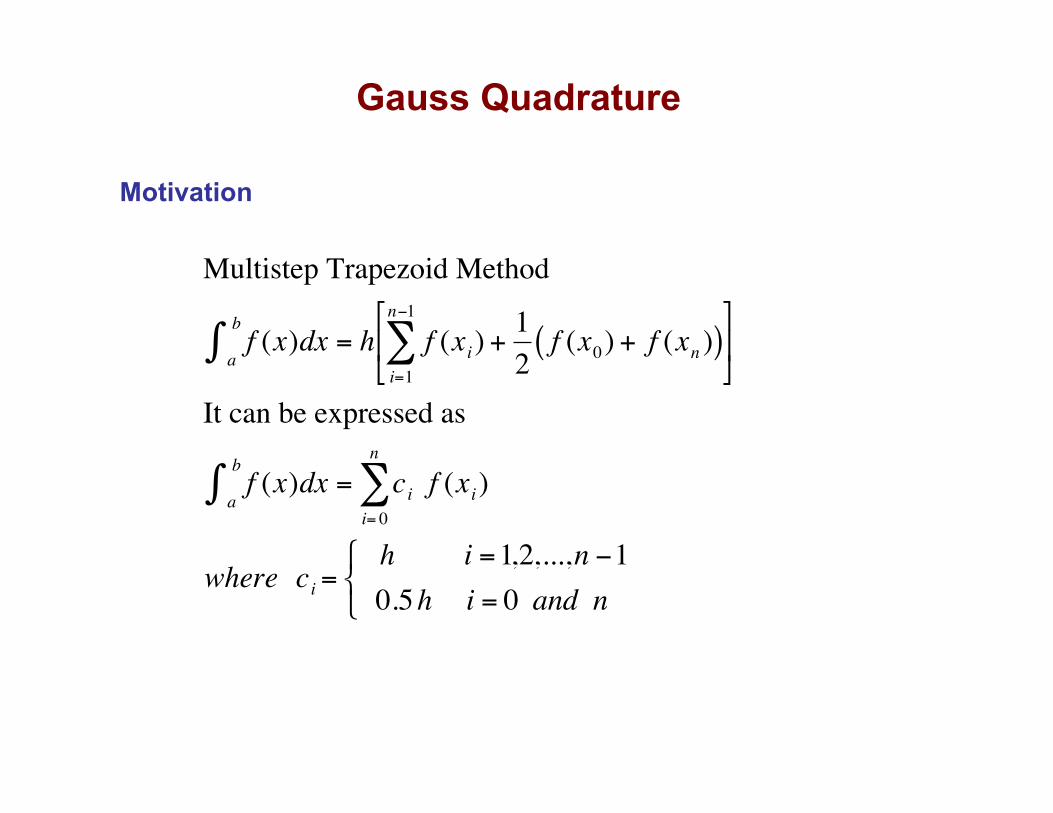
Gauss Quadrature

!

Multistep Trapezoid Method

f (x)dxa

b

" = h f (xi) +1

2f (x0) + f (xn )( )

i=1

n#1

$%

& '

(

) *

It can be expressed as

f (x)dxa

b

" = ci f (xi)i= 0

n

$

where ci =h i =1,2,...,n #1

0.5h i = 0 and n

+ , -

Motivation

!

f (x)dxa

b

" = ci f (xi)i= 0

n

#

ci :Weights xi :Nodes

Gauss Quadrature

Problem

How do we select ci and xi so that the formula gives abetter (higher order) approximation of the integral?

!

f (x)dx "a

b

# Pn (x)dxa

b

#where Pn (x) is a polynomial that interpolates f(x)

at the nodes x0,x1,...,xn

f (x)dx "a

b

# Pn (x)dxa

b

# = l i(x)i= 0

n

$ f (xi)%

& '

(

) * dx

a

b

#

+ f (x)dxa

b

# " ci f (xi)i= 0

n

$ where ci = l i(x)dxa

b

#

Approximate function with Polynomial

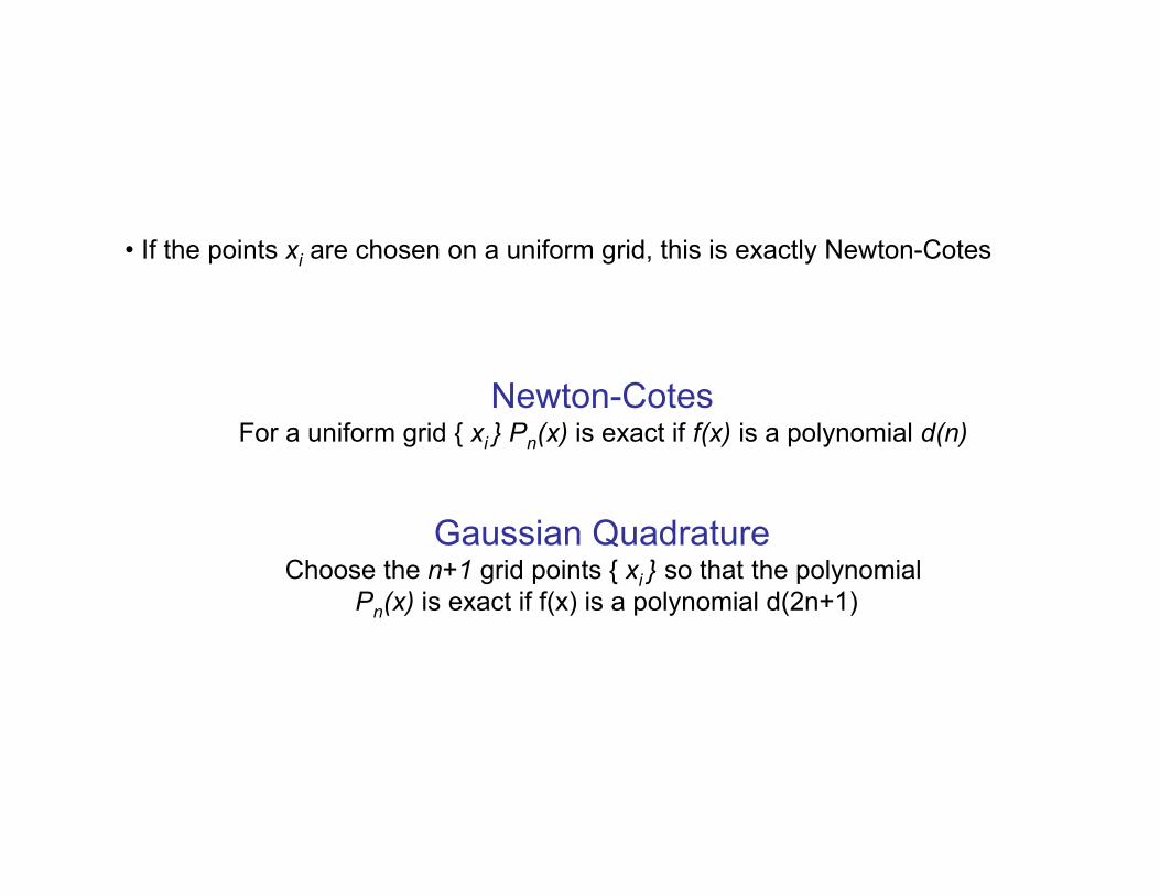
• If the points xi are chosen on a uniform grid, this is exactly Newton-Cotes

Newton-CotesFor a uniform grid { xi } Pn(x) is exact if f(x) is a polynomial d(n)

Gaussian QuadratureChoose the n+1 grid points { xi } so that the polynomial

Pn(x) is exact if f(x) is a polynomial d(2n+1)

!

"1

1

# f (x) dx = c0f (x

0) + c

1f (x

1)

How do we get nodes and weights

Example:

Can we select nodes and weights so that a (n+1)=2 nodes allow usto write a formula that is exact for polynomials of degree (2n+1) = 3?

Brute Force:

Set up equations for all polynomials d(0) to d(2n+1) and solve for ci and xi

!

f (x) =1; c0

+ c1

="1

1

# 1 dx = 2

f (x) = x; c0x0

+ c1x1

="1

1

# x dx = 0

f (x) = x2; c

0x0

2+ c

1x1

2=

"1

1

# x2dx = 2 /3

f (x) = x3; c

0x0

3+ c

1x1

3=

"1

1

# x3dx = 2

Solve simultaneously, get

!

c0

= c1

=1

x0

= "1/ 3;x1

=1/ 3

Nodes and weights for larger n:

wikipedia.org

ci

For a range of integration other than [-1,1], change of variables

!

a

b

" f (y) dy =b # a

2 #1

1

" f (b # a

2x +

a + b

2)dx

What is my limits are not [-1,1]?

!

=b " a

2ci f (

b " a

2i=1

n

# xi +a + b

2)

( )

!!!

"

#

$$$

%

&

+=

=

''(

)**+

,+-'

'(

)**+

,+--

-

+--..

22

22

5.3

15.05.

3

15.0

1

1

5.5.1

0

2

1

2

1

ee

dtedxetx

Example

2 points

Advantages/Disadvantages

1. For functions that are smooth or approximately polynomial beatsNewton-Cotes in accuracy.

!

erf(1) =2

"e#x 2

0

1

$ dxwith n=3, get 5 correctsignificant places

2. Not easy to get error bounds (need to know derivative f2n+2).

3. Unlike Romberg Integration, we cannot successively refine (Gauss-Konrad tries to overcome that.)

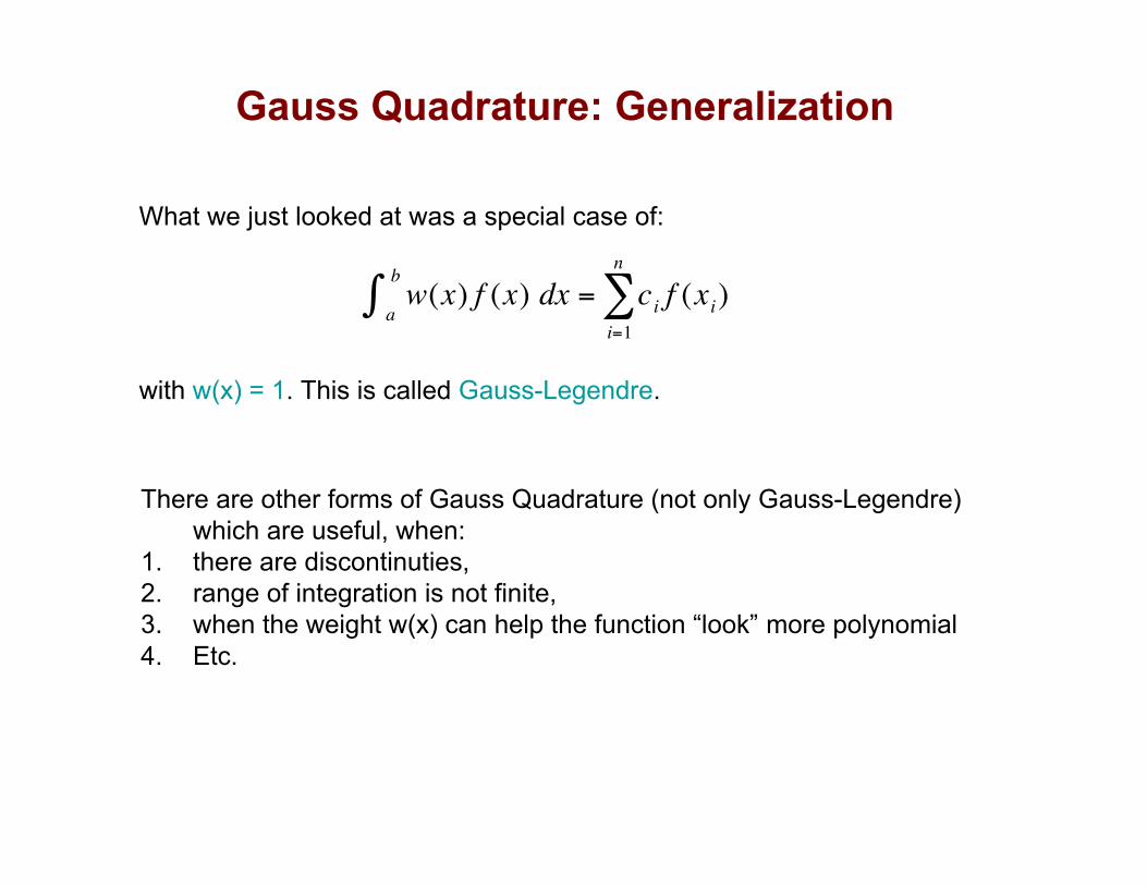
Gauss Quadrature: Generalization

What we just looked at was a special case of:

with w(x) = 1. This is called Gauss-Legendre.

!

a

b

" w(x) f (x) dx = ci f (xi)i=1

n

#

There are other forms of Gauss Quadrature (not only Gauss-Legendre)which are useful, when:

1. there are discontinuties,2. range of integration is not finite,3. when the weight w(x) can help the function “look” more polynomial4. Etc.

Generalization

The fundamental theorem of Gaussian quadrature states thatthe optimal nodes xi of the n-point Gaussian quadratureformulas are precisely the roots of the orthogonal polynomialfor the same interval and weighting function.

!

a

b

" w(x) f (x) dx = ci f (xi)i=1

n

#

Generalization

wikipedia

All we do are look for zeros of Pn(x) in [-1,1]. These are our xis.

The cis can be obtained from

!

ci=

2

(1" xi

2)( # P

n(x

i))2

Gauss-Legendre

In practice,

1. Gauss-Legendre is the most widely used Gauss quadrature formula.

2. We look at the limits and the weighting function w(x) for the integral wewant to evaluate and decide what quadrature formula might be best.

3. We don’t calculate the nodes and weights ourselves. Instead, we lookthem up for a give n, and simply carry out the weighted sum.

http://www.efunda.com/math/num_integration/num_int_gauss.cfm

4. Note that this may require a change of variables.

Generalization

Monte Carlo Integration

Adapting notes from David Kofke’sMolecular Simulation class.

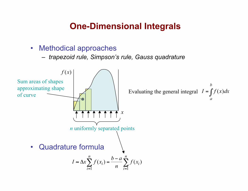
• Methodical approaches– trapezoid rule, Simpson’s rule, Gauss quadrature

• Quadrature formula

One-Dimensional Integrals

n uniformly separated points

Sum areas of shapesapproximating shapeof curve

( )

b

a

I f x dx= !Evaluating the general integral

1 1

( ) ( )n n

i i

i i

b aI x f x f x

n= =

!" # =$ $

( )f x

x

Monte Carlo Integration

• Stochastic approach• Same quadrature formula, different selection of points

• http://www.eng.buffalo.edu/~kofke/ce530/Applets/applets.html

1

( )n

i

i

b aI f x

n=

!" #

n points selected fromuniform distribution p(x)

( )x!

x

Random Number Generation

• Random number generators– subroutines that provide a new random deviate with each call– basic generators give value on (0,1) with uniform probability– uses a deterministic algorithm (of course)

• usually involves multiplication and truncation of leading bits of anumber

• Returns set of numbers that meet many statisticalmeasures of randomness– histogram is uniform– no systematic correlation of deviates

• no idea what next value will be from knowledge ofpresent value (without knowing generation algorithm)

• but eventually, the series must end up repeating

• Some famous failures– be careful to use a good quality generator

1 ( )modn nX aX c m+ = + linear congruential sequence

Plot of successivedeviates (Xn,Xn+1)

Not so random!

Random Number Generation

• RANDU– Linear congruential sequence developed in the 1960s at IBM

Not so random!http://www.purinchu.net/wp/2009/02/06/the-randu-pseudo-random-number-generator/

Errors in Random vs. Methodical Sampling

• Comparison of errors– methodical approach– Monte Carlo integration

• MC error vanishes much more slowly for increasing n• For one-dimensional integrals, MC offers no advantage• This conclusion changes as the dimension d of the

integral increases– methodical approach– MC integration

• MC “wins” at about d = 4

1//

dx L n! =independent of dimension!

for example (Simpson’s rule)

d = 236 points,361/2 = 6 ineach row

!

"I#$x 2 # n%2

!

"I# n$1/ 2

!

"I# n$2 / d

!

"I# n$1/ 2

Shape of High-Dimensional Regions

• Two (and higher) dimensional shapes can becomplex

• How to construct and weight points in a gridthat covers the region R?

2 2

2

( )

R

R

x y dxdy

rdxdy

+

=

!!

!!

Example: mean-squaredistance from origin

Shape of High-Dimensional Regions

• Two (and higher) dimensional shapes can becomplex

• How to construct and weight points in a gridthat covers the region R?

– hard to formulate a methodical algorithm in acomplex boundary

– usually do not have analytic expression forposition of boundary

– complexity of shape can increase unimaginablyas dimension of integral grows

2 2

2

( )

R

R

x y dxdy

rdxdy

+

=

!!

!!

Example: mean-squaredistance from origin

?iw

High-Dimensional Integrals

( )1 1!

( )N

N

N N U r

Z NU dr U r e

!"= #

Sample Integral from Statistical Physics

3Nparticle dimensional integral

• N=100 modest (course project) Therefore, in 3D, 300 dimensional integral

• Say 10 grid points in each dimension (very coarse) # function evaluations: 10300 (assume 1 flop)

• IBM BlueGene/L-system: 300 Tflop

• Total time: 10300/1015 ~10285 s = 10277 years

• Age of the universe: 1014

# atoms on earth: 1050

• N=100 modest (course project) Therefore, in 3D, 300 dimensional integral

• Say 10 grid points in each dimension (very coarse) # function evaluations: 10300 (assume 1 flop)

• IBM BlueGene/L-system: 300 Tflop

• Total time: 10300/1015 ~10285 s = 10277 years

• Age of the universe: 1014

# atoms on earth: 1050

High-Dimensional Integrals

( )1 1!

( )N

N

N N U r

Z NU dr U r e

!"= #

Sample Integral from Statistical Physics

3Nparticle dimensional integral

But we routinelycompute such

properties using MC

Integrate Over a Simple Shape? 1.

• Modify integrand to cast integral into asimple shaped region– define a function indicating if inside or

outside R

• Difficult problems remain– grid must be fine enough to resolve shape– many points lie outside region of interest– too many quadrature points for our high-

dimensional integrals (see applet again)

0.5 0.5 2 2

2 0.5 0.50.5 0.5

0.5 0.5

( ) ( , )

( , )

dx dy x y s x yr

dx dys x y

+ +

! !+ +

! !

+=" "

" "

1 inside R

0 outside R

s =!"#

•http://www.eng.buffalo.edu/~kofke/ce530/Applets/applets.html

• Statistical-mechanics integrals typically havesignificant contributions from miniscule regions of theintegration space

–

– contributions come only when no spheres overlap– e.g., 100 spheres at freezing the fraction is 10-260

• Evaluation of integral is possible only if restricted toregion important to integral– must contend with complex shape of region– MC methods highly suited to “importance sampling”

( )1 1!

( )N

N

N N U r

Z NU dr U r e

!"= #

( )0Ue

!" #

Integrate Over a Simple Shape? 2.

Importance Sampling

• Put more quadrature points in regions where integral receives itsgreatest contributions

• Return to 1-dimensional exampleMost contribution from region near x = 1

• Choose quadrature pointsnot uniformly, but accordingto distribution π(x)– linear form is one possibility

• How to revise the integral toremove the bias?

1

2

0

3I x dx= !

2( ) 3f x x=

( ) 2x x! =

The Importance-Sampled Integral

• Consider a rectangle-rule quadrature withunevenly spaced abscissas

• Spacing between points– reciprocal of local number of points per unit length

• Importance-sampled rectangle rule– Same formula for MC sampling

1

( )n

i i

i

I f x x=

! "#

1x!

2x!

3x!

nx!…1

( )i

i

b ax

n x!

"# =

Greater π(x) → more points → smaller spacing

1( )

( )

( )

ni

iix

b a f xI

n x!

!=

"# $ choose x points

according to π(x)

The Importance-Sampled Integral

!

"2 #

f

$

%

& '

(

) *

2

+f

$

%

& '

(

) *

2

n

Error in MC is related to the variance:

If f=constant, then numerator, and error vanish!

"2 #f2$ f

2

n

Can’t control the n-1/2

dependence

Choose π to make f/π approximately constant, then canmake error go to zero even if f is not constant.

Generating Nonuniform Random Deviates

• Probability theory says...– ...given a probability distribution u(z)– if x is a function x(z),– then the distribution of π(x) obeys

• Prescription for π(x)– solve this equation for x(z)– generate z from the uniform random generator– compute x(z)

• Example– we want on x = (0,1)– then– so x = z1/2

– taking square root of uniform deviate gives linearly distributed values• Generating π(x) requires knowledge of

( ) ( )dz

x u zdx

! =

( )x ax! =2 21

2z ax c x= + = a and c from “boundary conditions”

!

" (x)dx#

Generating Nonuniform Random Deviates

Example:

Generate x from linearly distributed random numbers between [a,b), π(x)

If π(x) is normalized then,

ba

π(x)

!

" (x) =2x

b2# a

2

If we have u(z) a uniform random number [0,1)

!

" (x) =2x

b2 # a2

=1dz

dx

dx

a

x

$2x

b2 # a2

= dz

0

z

$

x = a2

+ (b2 # a2)z

0 1

U(z)

Choosing a Good Weighting Function

• MC importance-sampling quadrature formula

• Do not want π(x) to be too much smaller or too much larger than f(x)– too small leads to significant contribution from poorly sampled region– too large means that too much sampling is done in region that is not (now)

contributing much

1( )

1 ( )

( )

ni

iix

f xIn x!

!=

" #

2x! =2

3x! =4

3x! =

( )x!

( )( )

f xx!

Variance in Importance Sampling Integration

• Choose π to minimize variance in average

• Smallest variance in average corresponds to π(x) = c × f(x)– not a viable choice– the constant here is selected to normalize π(x)– if we can normalize π(x) we can evaluate– this is equivalent to solving the desired integral of f(x)

• http://www.eng.buffalo.edu/~kofke/ce530/Applets/applets.html

( )x dx!"

222 1 ( ) ( )

( ) ( )( ) ( )

I

f x f xx dx x dx

n x x! " "

" "

# $% &% & % &' '= () *+ ,+ , + ,

- . - .- .' '/ 01 1

( )x! I"

n = 100 n = 1000

125n

0.09 0.03

2x18n

0.04 0.01

23x0 0 0

34x18n

0.04 0.01

2( ) 3f x x=

Summary• Monte Carlo methods use stochastic process to

answer a non-stochastic question– generate a random sample from an ensemble– compute properties as ensemble average– permits more flexibility to design sampling algorithm

• Monte Carlo integration– good for high-dimensional integrals

• better error properties• better suited for integrating in complex shape

• Importance Sampling– focuses selection of points to region contributing most to

integral– selecting of weighting function is important– choosing perfect weight function is same as solving integral

Extra Slides

!

li(x) =

"(x)

(x # xi) $ " (x

i)

"(x) = (x # x1)(x # x

2)..(x # x

n) = (x # x

i)

i= 0

n

%

Approximate function with Polynomial

!

Pn (x) = li(x)i= 0

n

" f (xi)

Recall, that the interpolating polynomial depends on the chosen grid points

Langrange interpolants can be written as,

!

limx"x

i

li(x) = lim

x"xi

#(x)

(x $ xi) % # (x

i)

=1Note that here,

!

" # (x i) = (xi $ x j )j= 0j% i

n

&

Theorem (Gauss)

Let P(x) be a nontrivial polynomial of degree n such that it is orthogonal topolynomials of lesser degree

!

a

b

" f (x)dx # ci f (xi)i= 0

n

$ where ci =a

b

" l i(x)dx!

a

b

" xkP(x)dx = 0 0 # k # n $1

If x0, x1, x2, …. xn are zeros of P(x) and

Then this approximation is exact for all polynomials ofdegree less than or equal to 2n+1

Method 2:

In practice, we use Gauss’ Theorem and well-studied classes of orthogonalpolynomials

Here, Legendre Polynomials (hence sometimes Gauss-Legendre Quadrature)

!

"1

1

# Pm(x)P

n(x)dx =

2

2n +1$nm

All we do are look for zeros of Pn(x) in [-1,1]. These are our xis.

The cis can be obtained from

!

ci=

2

(1" xi

2)( # P

n(x

i))2