
Numerical implementation of an Eulerian description of ...
144
Numerical implementation of an Eulerian description of finite elastoplasticity Dissertation zur Erlangung des Grades Doktor-Ingenieurin (Dr.-Ing.) der Fakult¨ at f¨ ur Bau- und Umweltingenieurwissenschaften der Ruhr-Universit¨ at Bochum von M. Sc. Marina Trajkovi´ c - Milenkovi´ c aus Leskovac, Serbien Bochum 2016
Transcript of Numerical implementation of an Eulerian description of ...
Numerical implementation of an Eulerian description
of finite elastoplasticity
Dissertation
zur
Erlangung des Grades
Doktor-Ingenieurin (Dr.-Ing.)
der
Fakultat fur Bau- und Umweltingenieurwissenschaften
der Ruhr-Universitat Bochum
von
M. Sc. Marina Trajkovic - Milenkovic
aus Leskovac, Serbien
Bochum 2016

Dissertation eingereicht am: 10.08.2016
Tag der mundlichen Prufung: 21.10.2016
Erster Referent: Prof. em. Dr.-Ing. Otto T. Bruhns
Zweiter Referent: Vertr.-Prof. Dr.-Ing. Ralf Janicke

To my little M.

Summary
The numerical implementation and validation of a self-consistent Eulerian consti-tutive theory of finite elastoplasticity, based on the logarithmic rate and additivedecomposition of the stretching tensor, via commercial finite element softwarehas been the objective of this thesis.
The elastic material behaviour has been modelled by a hypo-elastic relationwhile for the plastic behaviour an associated flow rule has been adopted. Inaccordance with the objectivity requirement, in the constitutive relations theobjective time derivatives have been used; the logarithmic rate, the Jaumannand Green-Naghdi rates as corotational rates and the Truesdell rate, the Ol-droyd rate and the Cotter-Rivlin rate as non-corotational rates.
It has been shown that for the large elastic deformation analysis the reliabilityof the Jaumann and Green-Naghdi rates decreases with the increased influenceof finite rotations while the non-corotational rates have to be excluded from theconstitutive relations. It has been proved that the implementation of the Log-rate successfully solves the so far existing integrability problem and the residualstress occurrence at the end of closed elastic strain cycles.
The constitutive relation for finite elastoplasticity based on the INTERATOMmodel has been developed and implemented. The obtained results have beencompared with the experimental records. The proposed constitutive model hasbeen proved as reliable for monotonic deformations while for cyclic deformationssome improvements remain to be implemented. The directions for improvementshave been given as well.

Zusammenfassung
Das Ziel dieser Arbeit sind die numerische Implementierung und die Validierungeiner selbstkonsistenten Eulerschen Beschreibung der finiten Elastoplastizitat,die auf der logarithmischen Rate und additiven Zerlegung des Dehnungstensorsbasiert. Implementierung und Validierung erfolgen in eine kommerzielle FiniteElemente Software.
Das elastische Materialverhalten wird durch eine hypo-elastisch Beziehung mod-elliert, wahrend fur das plastische Verhalten eine assoziative Fließregel angenom-men worden ist. Entsprechend der Forderung nach Objektivitat der konstitu-tiven Gleichungen sind objektive Zeitableitungen verwendet worden; und zwardie logarithmische Rate, die Jaumann Rate und die Green-Naghdi Rate alsmitrotierende und die Truesdell Rate, die Oldroyd Rate und die Cotter-RivlinRate als nicht-mitrotierende Raten Zeitableitungen.
Es wird gezeigt, dass fur große elastische Verformungen die Genauigkeit derZeitableitungen nach Jaumann und Green-Naghdi mit zunehmendem Einflussgroßerer Rotationen abnimmt, wahrend die nicht-mitrotierenden Zeitableitun-gen als ungeeignet aus konstitutiven Beziehungen auszuschließen sind. Mit Hilfeder logarithmischen Rate konnte das bisher ungeloste Integrabilitatsproblemgelost und das Auftreten von Eigenspannungen am Ende geschlossener elastis-cher Beanspruchungszyklen vermieden werden.
Das verwendete Materialgesetz fur die finite Elastoplastizitat baut auf dem IN-TERATOM Modell auf und wurde hier an ein vereinfachtes Materialverhaltenangepasst und implementiert. Die erhaltenen Ergebnisse wurden mit experi-mentellen Ergebnissen verglichen. Das vorgeschlagene Materialgesetz kann furmonotone Verformungen als zuverlassig angesehen werden. Fur zyklische Verfor-mungen dagegen werden einige Verbesserungen als notwendig erachtet. MoglicheVerbesserungsvorschlage werden gegeben.

Acknowledgments
I would like to express my sincere gratitude to Prof. em. Dr.-Ing. Otto T.Bruhns for giving me the privilege to work in this area and for his guidancethroughout my work on this thesis. I really appreciate his warm hospitality dur-ing my research stays at the Institute of Mechanics of the Ruhr University inBochum.
I want to thank to Vertr.-Prof. Dr.-Ing. Ralf Janicke for his acceptance to bethe co-reviewer of my thesis.
I also want to thank to Prof. Dr.-Ing. Rudiger Hoffer for beeing the facultyreviewer of my thesis.
My sincere gratitude to Prof. Dr Dragoslav Sumarac, my co-advisor, for hissupport and fruitful cooperation all these years.
I also want to thank to Prof. Dr.-Ing. Gunther Schmid, Prof. Dr.-Ing. RudigerHoffer and Prof. Dr Stanko Brcic for their advice and motivation.
Being the guest researcher at the Institute of Mechanics of the Ruhr Universityin Bochum was the extremely valuable experience for me. For co-financing mystays in Bochum I deeply appreciate the DAAD grants obtained through theSEEFORM programme. I want to thank to Prof. Dr. Heng Xiao and Dr.-Ing.Albert Meyers for very useful discussions while I was doing the first steps towardthis goal. I want to thank to all members of the (former) Chair of Technical Me-chanics for friendly and pleasantly working atmosphere. My special thanks toour small Serbian community in Bochum for their help.
I really appreciate the support of my friends and colleagues from the Faculty ofCivil Engineering and Architecture in Nis. Many thanks for my colleagues fromthe Faculty of Mechanical Engineering in Nis for fruitful discussions.
Finally, I want to thank to my parents, my sister and her family, and mostly tomy son and husband for their constant support, love and encouragement.
Bochum, 2016 Marina Trajkovic Milenkovic

Contents
List of Figures iv
List of Tables vii
Conventions and Notations viii
1 Introduction 11.1 Motivation . . . . . . . . . . . . . . . . . . . . . . . . . . . . . . 21.2 Aim of the thesis . . . . . . . . . . . . . . . . . . . . . . . . . . . 41.3 Outline . . . . . . . . . . . . . . . . . . . . . . . . . . . . . . . . 4
2 Deformation and motion 52.1 Introduction . . . . . . . . . . . . . . . . . . . . . . . . . . . . . . 52.2 Kinematics of deformable body . . . . . . . . . . . . . . . . . . . 5
2.2.1 Configurations and body motion . . . . . . . . . . . . . . 52.2.2 Lagrangian and Eulerian description . . . . . . . . . . . . 72.2.3 Material and spatial time derivative . . . . . . . . . . . . 9
2.3 Analysis of deformation . . . . . . . . . . . . . . . . . . . . . . . 102.3.1 Deformation gradient . . . . . . . . . . . . . . . . . . . . 102.3.2 Polar decomposition . . . . . . . . . . . . . . . . . . . . . 11
2.4 Analysis of strain . . . . . . . . . . . . . . . . . . . . . . . . . . . 132.4.1 Generalized strain measures . . . . . . . . . . . . . . . . . 13
2.5 Analysis of motion . . . . . . . . . . . . . . . . . . . . . . . . . . 152.5.1 Velocity gradient . . . . . . . . . . . . . . . . . . . . . . . 152.5.2 Rate of deformation . . . . . . . . . . . . . . . . . . . . . 172.5.3 Vorticity tensor . . . . . . . . . . . . . . . . . . . . . . . . 17
2.6 Objectivity of a tensor field . . . . . . . . . . . . . . . . . . . . . 192.6.1 Lagrangian and Eulerian objectivity . . . . . . . . . . . . 192.6.2 Objective time derivatives . . . . . . . . . . . . . . . . . . 202.6.3 Corotational and convective frame . . . . . . . . . . . . . 212.6.4 Non-corotational rates . . . . . . . . . . . . . . . . . . . . 232.6.5 Corotational rates . . . . . . . . . . . . . . . . . . . . . . 25
2.7 Decomposition of finite deformation . . . . . . . . . . . . . . . . 29
3 Conservation equations and stress measures 323.1 Introduction . . . . . . . . . . . . . . . . . . . . . . . . . . . . . . 323.2 Conservation laws . . . . . . . . . . . . . . . . . . . . . . . . . . 32
i

ii
3.2.1 Conservation of mass . . . . . . . . . . . . . . . . . . . . . 323.2.2 Conservation of linear momentum and Cauchy’s first law
of motion . . . . . . . . . . . . . . . . . . . . . . . . . . . 333.2.3 Conservation of angular momentum and Cauchy’s second
law of motion . . . . . . . . . . . . . . . . . . . . . . . . . 353.3 Stress measures and stress rates . . . . . . . . . . . . . . . . . . . 36
3.3.1 Alternative stress measures . . . . . . . . . . . . . . . . . 363.3.2 Lagrangian field equations . . . . . . . . . . . . . . . . . . 383.3.3 Work rate and conservation of mechanical energy . . . . . 393.3.4 Stress rates . . . . . . . . . . . . . . . . . . . . . . . . . . 41
3.4 Conjugate stress analysis . . . . . . . . . . . . . . . . . . . . . . . 443.5 Weak form of balance of momentum . . . . . . . . . . . . . . . . 48
3.5.1 Principle of virtual work . . . . . . . . . . . . . . . . . . . 483.5.2 Rate of the weak form of balance of momentum . . . . . . 50
4 Constitutive relations 524.1 Introduction . . . . . . . . . . . . . . . . . . . . . . . . . . . . . . 524.2 Continuum thermodynamics . . . . . . . . . . . . . . . . . . . . . 53
4.2.1 First law of thermodynamics . . . . . . . . . . . . . . . . 544.2.2 Second law of thermodynamics and principle of maximum
dissipation . . . . . . . . . . . . . . . . . . . . . . . . . . 574.3 Decomposition of the stress power . . . . . . . . . . . . . . . . . 604.4 Hypo-elasticity . . . . . . . . . . . . . . . . . . . . . . . . . . . . 61
4.4.1 Hypo-elastic relation for De - From small to finite strains 614.4.2 Hyper-elastic potential . . . . . . . . . . . . . . . . . . . . 63
4.5 Plasticity . . . . . . . . . . . . . . . . . . . . . . . . . . . . . . . 654.5.1 Yield surface and loading condition . . . . . . . . . . . . . 674.5.2 Priniple of maximum plastic dissipation and its consequences 694.5.3 Eulerian description of finite plastic deformations . . . . . 71
4.5.3.1 Classical models from IA model . . . . . . . . . 75
5 Numerical results 775.1 Introduction . . . . . . . . . . . . . . . . . . . . . . . . . . . . . . 775.2 Hypo-elasticity . . . . . . . . . . . . . . . . . . . . . . . . . . . . 77
5.2.1 Finite simple shear . . . . . . . . . . . . . . . . . . . . . . 785.2.2 Plate with a hole in finite tension . . . . . . . . . . . . . . 835.2.3 Closed elastic strain path - Hypo-elastic cyclic deformation 85
5.2.3.1 Small rotations (ξ = 0.1) . . . . . . . . . . . . . 865.2.3.2 Moderate rotations (ξ = 1) . . . . . . . . . . . . 895.2.3.3 Large rotations (ξ > 1) . . . . . . . . . . . . . . 93
5.3 Elastoplasticity . . . . . . . . . . . . . . . . . . . . . . . . . . . . 1015.3.1 Small cyclic elastoplastic deformations . . . . . . . . . . . 1015.3.2 Finite elastoplastic deformations . . . . . . . . . . . . . . 107
5.3.2.1 Elastic - perfectly plastic . . . . . . . . . . . . . 108

iii
5.3.2.2 Elastic - linear kinematic hardening . . . . . . . 111
6 Concluding remarks 1166.1 Summary and conclusions . . . . . . . . . . . . . . . . . . . . . . 1166.2 Possible extensions of the present research . . . . . . . . . . . . . 117
Bibliography 119

List of Figures
2.1 Undeformed and deformed configuration of the material body . . 6
2.2 Material and spatial coordinate systems . . . . . . . . . . . . . . 8
2.3 Polar decomposition . . . . . . . . . . . . . . . . . . . . . . . . . 12
2.4 Velocity gradient . . . . . . . . . . . . . . . . . . . . . . . . . . . 16
2.5 Angular velocity vector . . . . . . . . . . . . . . . . . . . . . . . 19
4.1 Initial and succeeding yield surfaces and material stability . . . . 68
4.2 Loading condition, normality rule and convexity of the yield surface 68
5.1 Finite simple shear problem . . . . . . . . . . . . . . . . . . . . . 79
5.2 Shear stress vs shear strain with Log-rate: Hypo-elastic yield point 80
5.3 Normal stress vs shear strain at simple shear for various rates . . 82
5.4 Shear stress vs shear strain at simple shear for various rates . . 82
5.5 Plate with a hole in tension: Model . . . . . . . . . . . . . . . . . 83
5.6 Plate with a hole in tension: Undeformed and deformed configu-ration and normal stress distribution for large elastic deformation 84
5.7 Plate with a hole in tension: Normalized normal stress distribu-tion for large elastic deformation in the node with the maximumnormal stress . . . . . . . . . . . . . . . . . . . . . . . . . . . . . 84
5.8 Plate with a hole in tension: Normalized normal stress distribu-tion for large elastic deformation in the node with maximum shearstress . . . . . . . . . . . . . . . . . . . . . . . . . . . . . . . . . . 85
5.9 Deformation cycle . . . . . . . . . . . . . . . . . . . . . . . . . . 86
5.10 τ 11, τ 12 and τ 22 single cycle development, ξ= 0.1, η= 0.02 . . . 86
5.11 Enlarged representation of τ 12 at first cycle end, ξ= 0.1, η= 0.02 87
5.12 τ 11, τ 12 and τ 22 single cycle development, ξ= 0.1, η= 0.1 . . . . 88
5.13 τ 12 single cycle development, ξ= 0.1, η= 0.1 . . . . . . . . . . . 88
5.14 τ 11, τ 12 and τ 22 single cycle development, ξ=1, η=0.1 . . . . . . 89
5.15 τ 12 single cycle development, ξ=1, η=0.1 . . . . . . . . . . . . . 90
5.16 Enlarged representation of τ 12 at first cycle end, ξ=1, η=0.1 . . 91
5.17 Enlarged representation of τ 11 at first cycle end, ξ=1, η=0.1 . . 91
5.18 Hundred cycle stress development for corotational rates, ξ=1, η=0.1 92
5.19 τ 12 development for Jaumann rate, ξ=1, η=0.1 . . . . . . . . . . 92
5.20 Normal stress τ 11 and τ 22 single cycle development, ξ=5, η=0.1 93
5.21 Shear stress τ 12 single cycle development, ξ=5, η=0.1 . . . . . . 94
iv

v
5.22 Enlarged representation of τ 11 and τ 12 single cycle development,ξ=5, η=0.1 . . . . . . . . . . . . . . . . . . . . . . . . . . . . . . 94
5.23 Ten and hundred cycle stress development for the Logarithmicrate, ξ=5, η=0.1 . . . . . . . . . . . . . . . . . . . . . . . . . . . 95
5.24 Ten cycle stress development for the Jaumann rate UMAT, ξ=5,η=0.1 . . . . . . . . . . . . . . . . . . . . . . . . . . . . . . . . . 96
5.25 Ten cycle stress development for the Jaumann rate ABAQUS,ξ=5, η=0.1 . . . . . . . . . . . . . . . . . . . . . . . . . . . . . . 96
5.26 Hundred cycle stress development for the Jaumann rate, ξ=5, η=0.1 97
5.27 Ten cycle stress development for the Green-Naghdi rate, ξ=5, η=0.1 98
5.28 Hundred cycle stress development for the Green-Naghdi rate, ξ=5,η=0.1 . . . . . . . . . . . . . . . . . . . . . . . . . . . . . . . . . 98
5.29 Hundred cycle stress development for the Trusdell rate, ξ=5, η=0.1 99
5.30 Hundred cycle stress development for the Oldroyd rate, ξ=5, η=0.1 99
5.31 Hundred cycle stress development for the Cotter/Rivlin rate, ξ=5,η=0.1 . . . . . . . . . . . . . . . . . . . . . . . . . . . . . . . . . 100
5.32 Residual normal and shear stresses for the given rates, ξ=5, η=0.1 100
5.33 Monotonic tensile test, source: Westerhoff (1995) . . . . . . . . . 102
5.34 Uniaxial cyclic experiments with strain amplitudes ∆ε = 0.005,0.015 and 0.02, source: Westerhoff (1995) . . . . . . . . . . . . . 102
5.35 Numerical results vs monotonic tensile test . . . . . . . . . . . . 103
5.36 Comparison between computation and experiment for the loading-unloading-reloading case . . . . . . . . . . . . . . . . . . . . . . . 104
5.37 First two cycles of the stress-strain curve for various strain ranges,∆ε = 0.005, 0.015 and 0.02, respectively . . . . . . . . . . . . . . 104
5.38 Saturated cycles: numerical results (solid line) vs monotonic ten-sile test (dashed line), source: Westerhoff (1995) . . . . . . . . . 105
5.39 IA-model uniaxial cyclic response for ∆ε = 0.005, 0.015 and 0.02 106
5.40 Comparison of IA-model, linear and nonlinear kinematic harden-ing, with experimental record for strain range ∆ε = 0.02 . . . . 107
5.41 Normalised normal stress vs shear strain for elastic-perfectly plas-tic behaviour . . . . . . . . . . . . . . . . . . . . . . . . . . . . . 109
5.42 Normalized shear stress vs shear strain for elastic-perfectly plasticbehaviour and its enlarged representation . . . . . . . . . . . . . 109
5.43 Elastic-perfect plasticity: Normalized normal stress developmentand enlarged representation of the normalized shear stress devel-opment for real material parameters . . . . . . . . . . . . . . . . 110
5.44 Normalized normal stress vs shear strain for linear kinematic hard-ening plasticity, c0/r = 0.6 . . . . . . . . . . . . . . . . . . . . . 111
5.45 Normalized shear stress vs shear strain for linear kinematic hard-ening plasticity, c0/r = 0.6 . . . . . . . . . . . . . . . . . . . . . 112
5.46 Normalized shear stress vs shear strain for linear kinematic hard-ening plasticity, c0/r = 0.022 . . . . . . . . . . . . . . . . . . . . 113

vi
5.47 Normalized normal stress vs shear strain for linear kinematic hard-ening plasticity, c0/r = 0.022 . . . . . . . . . . . . . . . . . . . . 113
5.48 Normalized normal and shear stress vs shear strain for the mate-rial parameters according to Westerhoff (1995) . . . . . . . . . . 114
5.49 Plate with a hole in tension: Undeformed and deformed configu-ration and normal stress distribution for large elastoplastic defor-mation with linear kinematic hardening . . . . . . . . . . . . . . 115
5.50 Plate with a hole in tension: Normalized normal stress distri-bution for large elastoplastic deformation with linear kinematichardening . . . . . . . . . . . . . . . . . . . . . . . . . . . . . . . 115

List of Tables
2.1 Transformation and objectivity of kinematical quantities . . . . . 21
5.1 Residual shear stresses τ 12/2G for ξ= 0.1, η= 0.02 . . . . . . . . 875.2 Residual stresses after first cycle for ξ= 1, η= 0.1 . . . . . . . . . 905.3 Residual τ 12 compared to τ 12max in % for ξ= 1, η= 0.1 . . . . . 905.4 Residual stresses after 10 cycles for ξ = 10, η = 0.2 . . . . . . . . 101
vii

Conventions and Notations
Scalars (italics)
B Bodybi Distinct eigenvalue of the Cauchy-Green tensorsDp Plastic dissipationdv Volume element in the current configurationdV Volume element in the reference configurationdx Length of the spatial vector dxdX Length of the material vector dXE Young’s modulusEt Tangent modulusF Loading functionG Shear modulusJ Determinant of the deformation gradient (Jacobian determinant)m MassP ParticleP0 Initial position of the particlep Current position of the particleq Heat flux vectorQ Heatr Internal heat sources Specific entropyS Entropyt Timeu Specific internal energyU Internal energyw Stress power per unit volumewp Accumulated plastic workW Elastic potentialW Complementary elastic potentialxi Component of the position vector in the current configurationXα Component of the position vector in the reference configurationY0 Tensile yield strength
Scalars (Greek characters)
γ Shear strain
viii

ix
εpeqv Equivalent plastic strainκ Isotropic hardening variableΛ Plastic multiplierλ First Lame constantµ Second Lame constantν Poisson’s ratioθ Absolute temperatureρ Mass density in the current configurationρ0 Mass density in the reference configurationσij Component of the stress tensorσy Yield stressΣ Elastic potentialψ Specific Helmholtz free energy
Vectors (boldface roman)
b Current body force per unit massb0 Referential body force per unit massc Rigid body translation of the observerda Area element in the current configurationdA Area element in the reference configurationdl Load vector in the current configurationdL Load vector in the reference configurationdx Line element in the current configurationdX Line element in the reference configurationn Unit normal vector in the current configurationN Unit normal vector in the reference configurationo Origin in the current configurationO Origin in the reference configurationei Unit vector in the current configurationEα Unit vector in the reference configurationt Tractiont Traction boundary conditionsu Displacementδu Virtual displacementu Displacement boundary conditionsv Velocityδv Virtual velocityx Position vector in the current configurationX Position vector in the reference configuration
Vectors (Greek characters)
ω Angular velocity vector

x
Second order tensors (boldface roman)
1 Unit tensorA Eulerian tensorA0 Lagrangian tensora Finger tensorA Piola tensorB Left Cauchy-Green tensorBi Eigenprojection of the left Cauchy-Green tensorC Right Cauchy-Green tensorCi Eigenprojection of the right Cauchy-Green tensorD Stretching tensore Almansi-Eulerian strain tensorE Green-Lagrangian strain tensor
e(m) Eulerian strain tensor
E(m) Lagrangian strain tensorF Deformation gradienth Hencky strainL Velocity gradientP Nominal stress tensorQ Rotation tensorR Rotation tensor (polar decomposition)RLog Logarithmic rotation tensorS Second Piola Kirchhoff stress tensorT First Piola Kirchhoff stress tensorU Right stretch tensorV Left stretch tensorW Vorticity tensor
Second order tensors (Greek characters)
α Back stressε Linearized (engineering) strainπ Eulerian stress measureΠ Lagrangian stress measureσ Cauchy stress tensorσ∗ Corotational Cauchy stress tensorσ Finger tensorτ Kirchhoff stress tensorτ Shifted Kirchhoff stress tensorΩ Angular velocity tensorΩ Spin tensorΩJ Zaremba-Jaumann spin tensorΩR Polar spin tensor
xi
ΩLog Logarithmic spin tensor
Fourth order tensors (boldface roman)
C Elastic stiffness tensorH Hypo-elasticity tensorI Identity tensorK Elastic compliance tensor
Other symbols
B ConfigurationBt Current configurationB0 Reference configurationBt Intermediate configuration∂Bt Boundary of the body in Bt
∂B0 Boundary of the body in B0
∂uB0 Displacement boundary of B in B0
∂σB0 Traction boundary of B in B0
∂uBt Displacement boundary of B in Bt
∂σBt Traction boundary of B in Bt
∂vBt Boundary of B in Bt with prescribed velocityE Euclidean point spaceO Observer
Special symbols & functions
det Determinantdiv Divergence with respect to xg(·) Scale functionh(·) Spin functiongrad Gradient with respect to xGrad Gradient with respect to X∇ Gradient with respect to x∇0 Gradient with respect to Xsym(·) Symmetric part of a tensortr(·) Trace of a tensor(·)T Transpose of (·)(·)−1 Inverse of (·)˙(·) Material time derivative of (·)
(·)L Lie derivative of (·)
(·) Arbitrary objective time derivative of (·)5(·) Arbitrary objective non-corotational rate of (·)

xii
5(·)Ol (Upper) Oldroyd rate of (·)5(·)CR Cotter-Rivlin (lower Oldroyd) rate of (·)5(·)Tr Truesdell rate of (·)
(·) Arbitrary objective corotational rate of (·)
(·) J Zaremba-Jaumann rate of (·)
(·)GN Polar or Green-Naghdi rate of (·)
(·)Log Logarithmic rate of (·)· Scalar product: Double contraction× Vector product⊗ Dyadic product? Rayleigh productLHS Left-hand side of the equationRHS Right-hand side of the equation
Superscripts
(·)e Elastic(·)p Plastic(·)? Transformed(·)′ Deviator of tensorial quantity

1 Introduction
Contemporary theories, established to describe the behaviour of materials thatundergo elastoplastic deformations, usually belong to the group of phenomeno-logical theories which rather try to mathematically formulate the behaviour ofmaterials observed during the experiments than to really explain a complex phe-nomenon of plasticity. The latter is the topic of the physical theories of plasticitythat are beyond the scope of this treatise. Application of the phenomenologicaltheories is extremely valuable in engineering practice such as in structural designor metal forming.
Engineering structure elements during their serviceability period are usually ex-posed to small strains with rare exceptions. But during their manufacturingmaterials could undergo very large strains usually accompanied with very largerotations, such as metals during metal forming. Even though the phenomenolog-ical models have been established and very well elaborated for the case of smalldeformations, especially for metals, finite elastoplastic deformations represent awide and yet not fully discovered field of research.
Nowadays powerful tools of numerical simulations help engineers in resolvingthe existing problems. Wide application of numerical simulations significantlyshortened the time required to obtain the final product and therefore made themanufacturing process less expensive. For example, until recently the design ofmetal forming was based on the knowledge earned trough a long practical expe-rience or expensive experimental try-outs. Nowadays, finite element simulationsare involved from the early stage of the production process. Each stage in thisprocess can be simulated and the errors can be corrected and avoided prior tothe actual manufacturing. The implemented theories can be tested, improvedand finally accepted for wide practical applications.
New achievements in the field of material sciences result with the introduction ofnew materials, such as shape memory alloys and composites, in the wide rangeof applications from medical purpose to numerous engineering structures. Incivil engineering structures shape memory alloys can be used for devices likedampers and base isolators. On the other hand, some known materials, such asthe rubber-like materials, see their use expanded beyond their traditional pur-pose, for example in civil engineering structures as a part in building supportsto protect the structure during the dynamic excitations. Having in mind thatone of the main tasks of engineers is to provide the reliable lifetime assessmentprocedures of engineering structures, the establishment of the constitutive the-
1

2 Chapter 1. Introduction
ory seems to be a complex, demanding and challenging process especially if thematerials are exposed to large deformations.
The more reliable and accurate constitutive model we want to establish, themore material parameters have to be introduced and defined. Since the experi-mental tests concerning large deformations are very difficult to perform and canbe followed by different unpredictable instabilities, there is a lack of a sufficientnumber of experiments necessary for the material parameter identification. Forexample, the large simple shear problem is used very often in numerical calcu-lations since it involves as much rotation as stretching. From this example wecan conclude the validity range of the proposed constitutive models. But, ”theexperimental execution of a simple glide test, that allows one, in principle, todiscriminate between models, is confronted with great difficulties as deformationbecomes heterogeneous rather quickly, so that there remains a lot of mysteriesto be elucidated concerning very large strains” (Besson et al., 2009).
1.1 Motivation
Concerning the finite strains, in order to fulfil the material frame indifference inthe constitutive model instead of a material time derivative objective rates haveto be implemented. The occurrence of the large rotations, such as in the afore-mentioned large simple shear example, can cause totally different material stressresponses for different stress rates introduced in the same constitutive model.Some of these results can be inconsistent with the experimental or theoreticalpredictions.
Looking back to history, Hencky was the first who has realized that for the fi-nite deformations analysis in an Eulerian description the time derivative mustbe independent of the respective rigid-body rotation, i.e. in the present notionmust be objective. He replaced the material time derivative with an expressionsimilar to that presently known as a Jaumann rate.
Unfortunately, this idea of Hencky has to wait for two decades to be reconsid-ered. Oldroyd was Hencky’s successor in developing the idea of the materialtime derivative replacement with, in his approach, ”convected differentiationwith respect to time” in the finite deformation problems and he formulated fourdifferent relations of the Cauchy stress derivatives (for more details and refer-ences the reader is referred to Bruhns, 2014).
The Prandtl-Reuss theory of elastoplastic material behaviour, adopted here, im-plies the additive decomposition of an increment (rate) of a total deformation intoits elastic and plastic parts. The deficiency of the constitutive law formulatedin rates of stresses and deformation for purely elastic processes, later denotedas hypo-elastic by Truesdell, has been firstly observed by the same author. It

1.1. Motivation 3
can be demonstrated by the occurrence of the residual stresses at the end of aclosed elastic cyclic process. Much later this was the topic of investigation ofvarious researchers, some of them are Kojic & Bathe (1987), Lin et al. (2003),Xiao et al. (2006b).
When a shear oscillatory phenomenon has been discovered and proved by Lehmann(1972), Dienes (1979) and Nagtegaal & de Jong (1982), i.e. it was shown that thehypo-elasticity model based on the Jaumann rate gives the unstable response atsimple shear, it has been concluded that for the case of large rotation the Jau-mann rate cannot be an appropriate choice. In the work of Simo and Pister(cf. Simo & Pister, 1984) it has been shown also that for the case of pure elasticdeformation, where the natural deformation rate is equal to its elastic part, noneof the constitutive hypo-elastic relations, based on at that time known objectiverates, fulfil the requirement that is exactly integrable to give an elastic relation.
In Besson et al. (2009) it has been shown that for the simple shear problem theoscillatory stress response occurs for the Jaumann rate if the elastic behaviour ofmaterials is taken into account. For pure plastic behaviour with isotropic harden-ing the shear oscillation vanishes while for the linear kinematic hardening it stillexists. Only for adopted nonlinear kinematic hardening for pure plasticity theoscillation in the stress response disappears. For elastoplastic behaviour of ma-terials even for isotropic hardening the stress response has oscillatory characterwhile its occurrence for adopted elastic-nonlinear kinematic hardening behaviouris sensitive on the hardening modulus and shear modulus ratio. For usual valuesof this ratio the oscillation in stress response exists.
These problems have been solved not long ago with the introduction of the so-called logarithmic rate. In Bruhns et al. (1999), Xiao et al. (1997a, 1997b, 1999)the authors proved the correctness of Log-rate implementations in the constitu-tive models for finite elastoplasticity.
But even though Jaumann himself pointed out the lacks of his rate, i.e. he”states that the behaviour of this rate material is indeed not elastic and onlyin the limit of infinitesimal deformations changes to that of an elastic body”(Bruhns, 2014), this time derivative has been widely accepted. The Jaumannrate accompanied with the Green-Naghdi rate is incorporated in all commercialfinite element codes for structural analysis especially for the case of finite defor-mations which caused a lot of debates among researches in last decade (see forexample Bazant et al., 2012, and Bazant & Vorel, 2014).
The aim of this thesis is to provide a contribution in this field of finite elasto-plastic deformation analysis.

4 Chapter 1. Introduction
1.2 Aim of the thesis
The main goal of this treatise is to implement the various widely used stress ratesas well as the recently introduced logarithmic rate into the proposed constitu-tive models of finite elasticity and elastoplasticity, based on the Prandtl-Reusstheory, via the commercial finite element software in order to examine the rangeof validity of the tested rates separately.
The second goal of this thesis is to test the new constitutive model for finiteelastoplastic deformations based on the INTERATOM model originally estab-lished for small deformation case (see Bruhns et al., 1988).
1.3 Outline
This thesis has been organized in six Chapters.
After this introduction, the basic relations of the non-linear continuum mechan-ics necessary for finite deformation description have been presented in the secondChapter. The objectivity principle has taken a prominent place in this Chapterbecause of its crucial role in the Eulerian description of physical processes. Theobjective time derivatives have been introduced and elaborated in detail.
The third Chapter, after a short review of the conservation laws, presents var-ious Lagrangian and Eulerian stress measures and defines several mostly usedobjective corotational and non-corotational rates. The special attention has beenassigned to the work conjugacy analysis from which the direct relation betweenthe rate of deformation tensor and the Eulerian Hencky strain has been obtained.A brief description of the weak form of the balance of momentum has been givenas well.
In the fourth Chapter the constitutive relations, based on the consistent Euleriantheory of finite elastoplasticity, have been presented and the advantage of thelogarithmic rate implementation in the proposed constitutive models has beenclarified.
The fifth Chapter shows the results obtained from the numerical implementationof the various objective stress rates, through the proposed constitutive models,in the commercial finite element code ABAQUS/Standard using the UMAT sub-routine.
The main conclusions and some possible extensions of the present research workhave been given in the last, sixth Chapter.

2 Deformation and motion
2.1 Introduction
The aim of this Chapter is to provide a brief review on kinematics of non-linearcontinuum mechanics necessary for the subsequent Chapters. For an elaboratedoverview of continuum mechanics, the reader is referred to Malvern (1969), Mars-den & Hughes (1983), Ogden (1984), Haupt (2000), Basar & Weichert (2000).
2.2 Kinematics of deformable body
2.2.1 Configurations and body motion
Even though in physical reality material body is a discontinuous system whichconsists of molecules and atoms, from the engineering point of view, materialbody can be considered as continuum where each particle of the body retains allphysical properties of the parent body.
The continuum model for material bodies is acceptable to engineers for two verygood reasons. The characteristic dimensions of the scale in which we usuallyconsider bodies of steel, aluminium, concrete, etc., are extremely large in com-parison with molecular distances so the continuum model provides a very usefuland reliable representation. Additionally, our knowledge of the mechanical be-haviour of materials is based almost entirely upon experimental data gatheredby tests on relatively large specimens (Mase & Mase, 1999).
Therefore, the deformable body of interest B, depicted in Fig. 2.1, may be con-sidered as a set of continuously distributed material points or particles P ∈ Boccupying the region B of the Euclidian point space E . This one-to-one mappingis termed a configuration of B. As the body moves, the region B changes ac-cordingly. The set of configurations depending on a parameter t, time interval,represents a motion of the body B.
A domain of the body at initial time, t = 0, is termed an initial configurationand denoted B0. A place P0 ∈ E , occupied at initial time by the material pointP ∈ B, is defined with the aforementioned mapping denoted by χ0 according tothe relation
P0 = χ0(P ), (2.1)
as it is presented in Fig. 2.1.
5

6 Chapter 2. Deformation and motion
A region of E occupied by B at present time is termed a current or Eulerianconfiguration and denoted Bt. The current position p of the material point P isdefined by a mapping χ
p = χ(P, t), (2.2)
where the function χ as well as its inverse function χ−1 must be continuous andat least twice continuously differentiable.
The motion of the body is defined with respect to the reference or Lagrangianconfiguration. The reference configuration does not need to be the initial config-uration or any configuration that was occupied by the material body during theprocess of deformation. But having in mind that all variables are defined withrespect to the reference configuration it is always convenient that the initial andreference configurations are identical, as it has been assumed here.
The process of deformation from the reference to the current configuration in-
Figure 2.1: Undeformed and deformed configuration of the material body
cludes changing in shape and position of the body of interest. While the formerleads to a varying distance between the arbitrary pairs of particles of the body,the latter reflects a rigid body motion. Both of these phenomena can be ob-served by one or several physical observers and, therefore, can be described indifferent ways. But, unlike their kinematical description, physical phenomenado not depend on the choice of the observer. That reflects on the mathematicalformulation of physical laws as constitutive models, developed later.

2.2. Kinematics of deformable body 7
An observer O monitors the deformation process from his position o ∈ E . Ifin the origin o we assume the Cartesian coordinate system with basis ei, theposition of the point p, occupied by the material point P in Bt, can be describedwith a position vector x by the relation
x = xiei, (2.3)
as it is depicted in Fig. 2.2. In the last relation the Einstein’s summationconvention has been used.
The vector x designates a deformed position of the material point P . The pair(x, t), recorded by O, is termed an event. Components of the vector x, xi inequation (2.3), are called current, spatial or Eulerian coordinates of the pointp. Italic indices in the further text will be used for the presentation of vector ortensor components in the current configuration.
The position vector of point P0, X, in the reference configuration, described by
X = XαEα, (2.4)
represents an undeformed position of the material point P . In equation (2.4)basis of the Cartesian coordinate system in the origin O are designated with Eα,while Xα are called referential, material or Lagrangian coordinates of the pointP0. Greek character indices in the further text will be used for the presentationof vector or tensor components in the reference configuration.
The motion of the body can now be described by
x = ϕ(X, t), (2.5)
where the function ϕ(X, t) maps the reference configuration into the currentconfiguration at time t and it is a one-to-one continuously differentiable andinvertible function, i.e.
X = ϕ−1(x, t). (2.6)
2.2.2 Lagrangian and Eulerian description
A scalar, vector or tensor field can be defined by either material or spatial coor-dinates as independent variables. For example, a displacement u of the materialpoint P from its position in B0 to its position in Bt, depicted in Fig. 2.2, can beexpressed in terms of X by
u(X, t) = c + x−X = c(X, t) +ϕ(X, t)−X, (2.7)
or in terms of x
u(x, t) = c + x−X = c(x, t) + x−ϕ−1(x, t), (2.8)

8 Chapter 2. Deformation and motion
Figure 2.2: Material and spatial coordinate systems
where Eqs. (2.5) and (2.6) have been used.
For the sake of simplicity and clarity, a vector c, representing the distance be-tween the origins O and o, will take the zero value. The displacement u in thematerial and spatial description is then respectively given by relations
u(X, t) = x−X = ϕ(X, t)−X, (2.9)
u(x, t) = x−X = x−ϕ−1(x, t). (2.10)
Equations (2.9) and (2.10) have different physical meanings. While the formerexpresses the displacement of the particle with the position vector X in B0 atcurrent time t, the letter is the displacement of any particle which is currently atthe position x. These two approaches in describing physical fields are known asthe material or Lagrangian description and the spatial or Eulerian description,respectively. The Lagrangian description refers to the behaviour of a materialparticle, whereas the Eulerian description refers to the behaviour at a spatialposition. The choice of the description depends on the nature of the problemunder consideration. In this treatise the Eulerian description has been adopted.
If a tensor is completely defined in the Lagrangian configuration it is labelled

2.2. Kinematics of deformable body 9
a Lagrangian tensor, while an Eulerian tensor is completely defined in the cur-rent configuration. A second-order tensor field, defined in both, the referenceand current configuration, is termed a two-point or mixed Eulerian-Lagrangiantensor.
2.2.3 Material and spatial time derivative
In the material description a velocity vector is the rate of change of the positionvector for a particle of interest, i.e. the time derivative with X held constant.Time derivatives with X held constant are termed material time derivatives,Lagrangian, total derivatives or shortened material derivatives.
v(X, t) =dϕ(X, t)
dt=
du(X, t)
dt≡ u. (2.11)
An acceleration of the material point in the Lagrangian description is then de-fined as the rate of change of the velocity, or the material time derivative of thevelocity, and can be written as
u(X, t) =d2u(X, t)
dt2=
dv(X, t)
dt≡ v. (2.12)
A superposed dot denotes the material time derivative or ordinary time deriva-tive when the variable is only a function of time.
When a variable is given in an Eulerian description, i.e. it is expressed in terms ofspatial coordinates and time, the material time derivative, designated as d(•)/dtat fixed X, is obtained by the chain rule for partial derivatives
˙(•) =d(•)dt|X
=∂(•)∂t|x
+ v · grad(•), (2.13)
where v is the velocity given in the spatial description and grad(•) representsthe gradient with respect to the spatial coordinates. In the RHS of Eq.(2.13) thefirst term is a spatial time derivative or Eulerian time derivative, and the secondis a convective or transport term. For details see Belytschko et al. (2000).
As an example, the material time derivatives of the velocity v(x, t) and tensorfunction σ(x, t) will be given by relations
u(x, t) = v(x, t) =∂v(x, t)
∂t+ v(x, t) · ∂v(x, t)
∂x, (2.14)
σ(x, t) =∂σ(x, t)
∂t+ v(x, t) · ∂σ(x, t)
∂x. (2.15)

10 Chapter 2. Deformation and motion
2.3 Analysis of deformation
2.3.1 Deformation gradient
The distance between two close material points P0 and Q0 in the reference con-figuration is determined by the material vector dX (see Fig. 2.2). During theprocess of deformation this elemental material vector is transforming in a corre-sponding space vector dx according to the law
dx = F · dX. (2.16)
A tensor F that describes such a kind of transformation is called a deformationgradient. It is a two-point tensor that lives partially in the reference configura-tion and partially in the current configuration and it can be represented by therelation
F =∂ϕ(X, t)
∂X=
∂xi∂Xα
ei ⊗Eα = (Grad x)T , (2.17)
where the operator Grad(•) represents a gradient with respect to the materialcoordinates.
Since one spot in space can be occupied by not more than one material point,meaning ϕ is a one-to-one mapping between X and x, the deformation gradientF is always a revertible tensor, i.e.
dX = F−1 · dx. (2.18)
Therefore, and from the reason to avoid physically unrealistic case where thedeformation reduces the length of a line element to zero, a Jacobian determinantof the tensor F, or shortly Jacobian, J has to have a non-zero value, i.e.
J = det(F) 6= 0. (2.19)
In most of research literature, relation (2.16) is called a push forward transfor-mation and the space vector dx is the push forward equivalent of the materialvector dX. Inversely, relation (2.18) is called a pull back transformation and thematerial vector dX is the pull back equivalent of the space vector dx.
Similarly to the previously explained line element transformation, according tothe Nanson’s formula (cf. Ogden, 1984), a referential surface element dA canbe transformed to its current representation da, i.e.
da = JF−T · dA. (2.20)
An elemental volume dV in the reference and its corresponding volume dv inthe current configuration are related to each other by the Jacobian as
dv = JdV. (2.21)

2.3. Analysis of deformation 11
From the last equation one additional mathematical requirement for J is thatit must be non-negative. Regarding the last statement and Eq. (2.19), we canconclude that
J > 0. (2.22)
The deformation at which J = 1 is called isochoric or volume preserving at X,as in a simple shear case.
2.3.2 Polar decomposition
Rotation, especially combined with deformation, is fundamental to nonlinearcontinuum mechanics. The most important theorem which elucidates the roleof rotation in large deformation problems is a polar decomposition theorem (seefor example Malvern, 1969).
Following this theorem, the deformation gradient F, as a non-singular second-order tensor, can be uniquely multiplicatively decomposed into a positive definitesymmetric second-order tensor V or U, and an orthogonal second-order tensorR such that
F = V ·R = R ·U, (2.23)
where the rotation tensor R is proper orthogonal, i.e.
RT = R−1 , RT ·R = R ·RT = 1 with det(R) = 1. (2.24)
From (2.24) it follows that
det(F) = det(V) = det(U). (2.25)
Tensors V and U are called left and right stretch tensors, respectively. V is anEulerian, and U is a Lagrangian tensor, while R is, as F, a two-point tensor.
In the case of a rigid body motion F = R and U = V = 1, where 1 representsa symmetric unit tensor of the second order. During the deformation whereU = V = F, the rotation tensor is a unit two-point tensor and that is thecase of a pure strain. In general, deformation consists of the rigid body motion,represented by R, and the stretching, represented by V, that is following therigid body motion. This decomposition of the deformation is termed a left polardecomposition. In a right polar decomposition the stretching, represented by U,is followed by the rigid body motion, as shown in Fig. 2.3 for one dimensionalelement dX.
The left stretch tensor V can be obtained from the right stretch tensor U byforward rotation with R and vice versa
V = R ?U = R ·U ·RT , U = RT ?V = RT ·V ·R. (2.26)

12 Chapter 2. Deformation and motion
Figure 2.3: Polar decomposition
A star product in the last relation is called a Rayleigh product and it describesa transformation between the Lagrangian and Eulerian configuration. There-fore, V is the Eulerian counterpart of the Lagrangian tensor U and U is theLagrangian counterpart of the Eulerian tensor V.
Even though V and U live in different configurations, from (2.26) it is obtainedthat their eigenvalues have the same values and, additionally, in accordance with(2.25) are equal to those of F, because all eigenvalues of R are equal to 1 (cf.Bruhns, 2005).
Sometimes it is more convenient to use the squares of V and U, termed as leftand right Cauchy-Green tensors and defined as
B = V2 = F · FT , C = U2 = FT · F. (2.27)
The relation between the Eulerian tensor B and its Lagrangian counterpart Ccan be defined as
B = R ?C , C = RT ?B. (2.28)

2.4. Analysis of strain 13
2.4 Analysis of strain
2.4.1 Generalized strain measures
If the distance dX, between any close material points P and Q (see Fig. 2.2),remains unchanged during the process of deformation, the deformable body Bis exposed to a rigid body displacement. Otherwise, the body B is deformedand the length dX becomes dx in the current configuration (cf. Lubliner, 2008).The difference between squares of distances between particles of interest in thereference and current configuration can be expressed in terms of material andspatial coordinates in the following way
|dx|2 − |dX|2 = dX · (FT · F− 1) · dX = 2dX ·E · dX (2.29)
and
|dx|2 − |dX|2 = dx · (1− (F · FT )−1
) · dx = 2dx · e · dx, (2.30)
where E and e are Lagrangian and Eulerian strain measures, respectively.
Variables that give us an insight into the deformation in the vicinity of any ma-terial point of the body are elongations (stretches) and shear strains. The setof all elongations and shear strains for all possible directions from one materialpoint defines a state of deformation at that point and can be described by dif-ferent either material or spatial strain tensors.
Based on the right and left stretch tensors U and V, Seth, 1964 and Hill (1968,1978) introduced a general class of Lagrangian and Eulerian strain tensors desig-nated by E(m) and e(m), respectively. Since the application of Cauchy-Green ten-sors C and B is more comfortable for numerical purposes due to their quadraticform, a modified definition of the general class of strain measures is given by
E(m) = g(C) =
n∑i=1
g(bi)Ci
e(m) = g(B) =
n∑i=1
g(bi)Bi,
(2.31)
where bi represents n distinct eigenvalues of tensors C and B, while Ci and Bi
are the corresponding eigenprojections (for details see Xiao et al., 1998b; Bruhns,2005).
The scale function g(•) is a smooth and monotonously increasing function withinitial conditions
g(1) = 0 and g′(1) =1
2, (2.32)

14 Chapter 2. Deformation and motion
where g′(•) is the first derivative of g(•). The scale function is defined as:
g(bi) =
1
2m(bmi − 1) for m 6= 0
12ln(bi) for m = 0,
(2.33)
(see Doyle & Ericksen, 1956, and Seth, 1964).
In this way, for different values of the parameter m, all commonly known strainmeasures can be obtained. For example, form = 1, from Eq. (2.31)1 the materialGreen-Lagrangian strain tensor can be derived
E =1
2
n∑i=1
(bi − 1)Ci =1
2(C− 1) =
1
2(U2 − 1), (2.34)
and from Eq. (2.31)2 the spatial Finger tensor comes as
a =1
2
n∑i=1
(bi − 1)Bi =1
2(B− 1) =
1
2(V2 − 1). (2.35)
For m = −1, the material Piola tensor comes from (2.31)1
A =1
2
n∑i=1
(1− bi−1)Ci =1
2(1−C−1) =
1
2(V2 − 1) (2.36)
and the spatial Almansi-Eulerian strain tensor
e =1
2
n∑i=1
(1− bi−1)Bi =1
2(1−B−1) =
1
2(1−V−2) (2.37)
can be obtained from (2.31)2.
In the special case, for m = 0, one can obtain a Hencky or Logarithmic straintensor in the Lagrangian
H =1
2
n∑i=1
lnbiCi =1
2lnC = lnU (2.38)
and Eulerian description
h =1
2
n∑i=1
lnbiBi =1
2lnB = lnV. (2.39)
The spatial and material logarithmic strain tensors h and H are also known astrue or natural strain measures and are of great importance in a finite elasto-plastic deformation description. One of their advantages compared with otherstrain measures is the additivity property of successive strains. Logarithmic

2.5. Analysis of motion 15
strain measures were disregarded for a long period even though Hencky intro-duced them in theoretical mechanics in 1928 (cf. Hencky, 1928, 1929a, 1929b).
Having in mind that rotations, accompanied with distortions, in the case of largedeformations have a prominent role, the strain measure appropriate for this kindof deformation calculation has to be dependent of the stretching but indepen-dent of the rigid body motion. All aforementioned strain measures satisfy thisrequirement.
As for any other corresponding pair of tensors in the referential and currentconfiguration, relation (2.28) can be applied for all strain tensors as well
e(m) = R ?E(m) and E(m) = RT ? e(m) (2.40)
2.5 Analysis of motion
The deformation gradient F, stretching tensors U and V, Cauchy-Green tensorsC and B and strain measures introduced in the last Section as well are quantitiesindependent of time. However, most of formulations of plastic behaviour ofmaterials (viscoplasticity is an obvious example) are given as functions of ratesof variables. Even a rate-independent model of plasticity is usually written ina rate form for a numerical implementation into finite element based programs.Therefore, it is necessary to reconsider how the aforementioned quantities canbe expressed in rate form, i.e. as functions of time.
2.5.1 Velocity gradient
The velocity of the material point, introduced in Section (2.2.3), is by nature anEulerian quantity even though in Eq. (2.11) it is expressed in terms of materialcoordinates. The velocity can be defined as a function of spatial coordinates aswell
v(t) = x =dx
dt. (2.41)
A velocity increment dv, which emerges by virtue of a spatial position changedx, in the same deformed configuration (cf. Fig. 2.4), can be written in the form
dv(x, t) =∂v(x, t)
∂x· dx. (2.42)
An Eulerian second-order tensor defined as
L =∂v(x, t)
∂x= ∇v (2.43)
16 Chapter 2. Deformation and motion
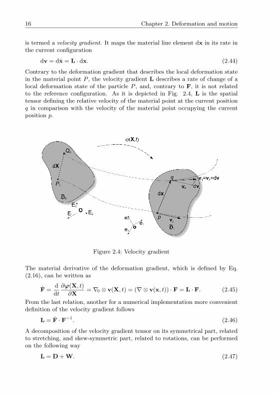
is termed a velocity gradient. It maps the material line element dx in its rate inthe current configuration
dv = dx = L · dx. (2.44)
Contrary to the deformation gradient that describes the local deformation statein the material point P , the velocity gradient L describes a rate of change of alocal deformation state of the particle P , and, contrary to F, it is not relatedto the reference configuration. As it is depicted in Fig. 2.4, L is the spatialtensor defining the relative velocity of the material point at the current positionq in comparison with the velocity of the material point occupying the currentposition p.
Figure 2.4: Velocity gradient
The material derivative of the deformation gradient, which is defined by Eq.(2.16), can be written as
F =d
dt
∂ϕ(X, t)
∂X= ∇0 ⊗ v(X, t) = (∇⊗ v(x, t)) · F = L · F. (2.45)
From the last relation, another for a numerical implementation more convenientdefinition of the velocity gradient follows
L = F · F−1. (2.46)
A decomposition of the velocity gradient tensor on its symmetrical part, relatedto stretching, and skew-symmetric part, related to rotations, can be performedon the following way
L = D + W. (2.47)

2.5. Analysis of motion 17
The tensor D is termed as a rate of deformation tensor or a stretching tensorand it can be calculated using the following formula
D =1
2(L + LT ) =
1
2(∇v + (∇v)T ), (2.48)
while the tensor W is named a vorticity tensor or a spin tensor, and can beobtained by the relation
W =1
2(L− LT ) =
1
2(∇v− (∇v)T ), (2.49)
(see Malvern, 1969, and Micunovic, 1990).
2.5.2 Rate of deformation
The material rate of the Green-Lagrangian strain tensor, given by Eq. (2.34),and using relation (2.27)2, can be determined in the following way
E =1
2C =
1
2(F
T · F + FT · F) =1
2FT · (L + LT ) · F = FT ·D · F. (2.50)
The last relation demonstrates that the material rate of deformation E repre-sents a pull-back equivalent of the Eulerian rate of deformation tensor D. Bothquantities define the rate of change of the scalar product of two elemental vectorsin the current configuration (cf. Bonet & Wood, 2008). While the latter givesthe rate of change in terms of elemental vectors in the current configuration, theformer gives the rate of change in terms of corresponding elemental vectors inthe reference configuration. We can conclude from here that E and D are theLagrangian and, respectively, Eulerian measure of the rate of change of the ma-terial line length as well as the rate of change of the angle between two materialline elements of interest, during the process of deformation.
Even though the aforementioned conclusions are generally accepted in nonlinearcontinuum mechanics, until recently it was considered that the stretching tensorD cannot be defined either as a Lagrangian or as an Eulerian strain rate tensorand therefore it was not considered as a rate of deformation (see Ogden, 1984).However, Xiao et al.( 1997b, 1998b) proved that the stretching tensor D can beintegrated to give the Hencky strain tensor h, defined in the Eulerian descriptionby relation (2.39).
2.5.3 Vorticity tensor
In order to understand better the nature of the vorticity tensor, which definesthe rotation of the body during deformation, further transformations will beperformed.

18 Chapter 2. Deformation and motion
The material rate of the deformation gradient, defined by polar decomposition(2.23)1, is given by
F = R ·U + R · U. (2.51)
Relation (2.46) can be now rewritten as
L = F ·F−1 = (R ·U+R · U) ·U−1 ·R−1 = R ·RT +R · U ·U−1 ·RT . (2.52)
The stretching and vorticity tensors are then given by relations
D =1
2R · (U ·U−1 + U−1 · U) ·RT (2.53)
and
W = R ·RT +1
2R · (U ·U−1 −U−1 · U) ·RT . (2.54)
The first term on the RHS of the last equation represents an angular velocitytensor and it depends on the rigid body rotation and its rate but not on thestretching of the body
Ω = R ·RT . (2.55)
As it can be seen from relations (2.53) and (2.54), decomposition of the ve-locity gradient on the vorticity and stretching tensor is evidently more compli-cated than decomposition of the deformation gradient on pure rotation and purestretching (see (2.23)). The reason for that lies in the fact that the vorticitytensor, apart from the rigid body rotation, depends on the elongation and elon-gation rate.
In the absence of deformation, i.e. in the case of a rigid body motion, D = 0,resulting in W = L = Ω . The increment of the relative velocity of the materialpoint Q, occupying the position q, in comparison with the velocity of the particleP , that occupies the position p, as it is depicted in Fig. 2.5, can then be definedas
dv = W · dx = ω × dx, (2.56)
where ω is the angular velocity vector obeying the rule
Ω · r = ω × r, (2.57)
for each vector r.

2.6. Objectivity of a tensor field 19
Figure 2.5: Angular velocity vector
2.6 Objectivity of a tensor field
As it was stated in Section 2.2.1, the same process of deformation can be moni-tored by two different observers O and O∗ that occupy different positions in thespace, o and o∗ respectively, and can move relative to one another. Moreover,the observers can monitor the same process with time difference, but they mustagree on the space and time distance recorded by them while they are followingthe movement of a same material point. Using the language of mathematics,there exists a one-to-one mapping between the event (x, t), recorded by O, andthe event (x∗, t∗) recorded by O∗. This mapping is termed a change of the ob-server or observer transformation (cf. Ogden, 1984) that is represented by therelation
x∗ = Q(t) · x + c(t) and t∗ = t− a, (2.58)
where Q is the proper orthogonal tensor of relative rotation and c is the vectorof relative translation of one observer relatively to another, while with the scalarquantity a time distance in records has been designated. This scalar quantitywill be disregarded in the further text, i.e. it will be considered that a = 0.
Physical processes are independent of an observer. Therefore a demand is thattensor fields (scalars, vectors or tensors of higher rank) that qualitatively andquantitatively describe those physical processes stay independent of the changeof the observer i.e. must stay objective.
2.6.1 Lagrangian and Eulerian objectivity
According to Ogden (1984), the objectivity feature depends on the configurationin which the quantity has been defined.
Scalar quantity α0 , vector α0 and second-order tensor A0, defined in the La-

20 Chapter 2. Deformation and motion
grangian configuration, are objective if they stay unchanged after the change ofthe observer, i.e.
α∗0(X, t∗) = α0(X, t)
α∗0(X, t∗) = α0(X, t)
A∗0(X, t∗) = A0(X, t).
(2.59)
Concerning Eulerian quantities, scalar α , vector α and second-order tensor A,are objective if they obey the following rules of transformation by virtue of thechange of the observer
α∗(x, t∗) = α(x, t)
α∗(x, t∗) = Q(t) ·α(x, t) = Q(t) ?α(x, t)
A∗(x, t∗) = Q(t) ·A(x, t) ·Q(t)T = Q(t) ?A(x, t).
(2.60)
For a Lagrange-Eulerian, or Euler-Lagrangian two-point tensor, defined as
A = α0 ⊗α, or A = α⊗α0 (2.61)
the objectivity criteria is defined as
A∗
= A ·QT , and A∗
= Q · A, (2.62)
respectively.
Based on the aforementioned transformation rules, in Table 2.6.1 the kinematicalquantities introduced in this Chapter and their transformed forms have beenpresented and their objectivity examined.It must be pointed out that if the Eulerian tensor is objective its corresponding
Lagrangian tensor is objective as well, and vice versa. (see Xiao et al., 1998c;Bruhns, 2005).
2.6.2 Objective time derivatives
If two coordinate systems are associated with the positions of the observersO andO∗, i.e. with o and o∗, respectively, transformation between O and O∗ can bealso determined as a change of frame. As it can be seen from Eq. (2.59)3, theLagrangian strain tensors are not affected by the change of the observer, i.e.by the change of frame. Thus, the material time derivative of the transformedLagrangian second-order tensor, given by the relation
A∗0 = A0, (2.63)
satisfies the objectivity requirement as well.
Contrary to the Lagrangian tensor, the objective Eulerian second-order tensor

2.6. Objectivity of a tensor field 21
QuantityTransformed quantity
ObjectiveLagrangian Eulerian Two-point
F F∗ = Q · F yesJ J∗ = J yesR R∗ = Q ·R yesV V∗ = Q ?V yesU U∗ = U yesB B∗ = Q ?B yesC C∗ = C yes
L L∗ = Q ? L + Q ·QT noD D∗ = Q ?D yes
W W∗ = Q ?W + Q ·QT no
Table 2.1: Transformation and objectivity of kinematical quantities
transforms according to (2.60)3 and therefore it is dependent of the change offrame. From that follows that the material time derivative of the objectiveEulerian second-order tensor will be transformed according to the relation
A∗
= ˙Q ?A =˙
Q ·A ·QT = Q ·A ·QT + Q · A ·QT + Q ·A · QT. (2.64)
From the last relation it turns out
A∗ 6= Q · A ·QT, (2.65)
and thus it can be concluded that the material time derivative of the objectiveEulerian second-order tensor is not an objective quantity. To preserve the ob-jectivity requirement in the Eulerian description one has to use instead of thematerial time derivative an objective time derivative that satisfies the relation
A∗
= Q ?A, (2.66)
whereA is the objective time derivative of the Eulerian second-order tensor A.
2.6.3 Corotational and convective frame
Let us consider that the observer O is located at the fixed point of space o, whilethe observer O∗ is situated on the moving body at point o∗ and it moves androtates together with the deformable body. The sitting point of the observer O,o, is the origin of a so-called fixed background frame, while o∗ is then the originof a so-called co-deforming frame. In that case relation (2.58) represents thetransformation between the background and co-deforming frame. That meansthat the pair (x,t) represents the point in the Galilean space-time, occupied by

22 Chapter 2. Deformation and motion
the particle P , observed by O from the background frame, while the pair (x∗,t)represents the same point in the space observed by O∗ from the transformedmoving frame. Both observers have recorded the position of the particle at thesame time, i.e. the time difference vanishes.
We will now rewrite relation (2.58) and assume transformation between theframes as
x∗ = K(t) · x + c(t) and t∗ = t, (2.67)
where the time dependent tensor K, is not a proper orthogonal but generalasymmetric second-order tensor determined by the following first-order differen-tial system with a prescribed initial value
K = Ψ ·K, K|t=0 = 1. (2.68)
In the previous relation Ψ is the asymmetric second-order tensor given by
Ψ = Ω + Γ, (2.69)
where Ω is the antisymmetric part and Γ is the symmetric part of Ψ. Theskew-symmetric tensor Ω is called a spin and has the properties of the angularvelocity Ω introduced in Section 2.5.3.Transformation of an objective Eulerian tensorial quantity A, defined in thebackground frame, to A∗ in the co-deforming frame can be determined by thefollowing transformation rule
A∗ = K ·A ·KT = K ?A. (2.70)
Accordingly, the material time derivative of the transformed quantity A∗ can bedefined as
A∗
= ˙K ?A = K ·A ·KT + K · A ·KT + K ·A · KT = K ?A, (2.71)
where the objective time derivative, introduced in the previous Section, is deter-mined by the tensor Ψ as
A= A + A ·Ψ + ΨT ·A. (2.72)
The kinematical property of relation (2.71) can be understood in such a waythat a material time derivative of a counter part of an Eulerian quantity A in aco-deforming frame, that is A
∗, is a co-deforming counter part of an objective
time derivative of the same quantity A in a background frame.
The objective rates of the symmetric Eulerian second-order field have been so
far given in a general formA. In modelling of various material behaviours, us-
ing the formulation with Eulerian rates, objective rates play an essential role.

2.6. Objectivity of a tensor field 23
Therefore, the type of the objective rate should be carefully chosen. Dependingon the choice of the tensor Ψ the objective rates can be generally classified intwo categories of corotational and non-corotational objective rates ( cf. Bruhnset al., 2004).
Whenever the symmetric part of Ψ, given by relation (2.69), vanishes, i.e. Ψbecomes equal to the spin Ω, the frame defined by Eqs. (2.67) and (2.68) is aspinning or corotating frame and K is then equal to the rotation tensor. Oth-erwise, Ψ determines a convective frame. While the former experiences onlyconstant rotation the latter can deform and rotate continuously during the de-formation process. In the case of a convective frame the coordinate system ino∗ is no longer a Cartesian coordinate system and under the change of frame aphysical or kinematical quantity can lose some important features. For example,the eigenvalues of the quantity of interest can be modified during the processof deformation. If we want to preserve the physical or kinematical features of aphysical or a kinematical tensor, the tensor Ψ must be a skew-symmetric tensor,meaning Ψ = Ω. That leads to K = Q, i.e. K is the proper orthogonal rotationtensor. For details see Bruhns et al. (2004) and Xiao et al. (2005). Integrationof (2.71) leads to the generalised objective time integration of the objective rate
A = K−1 ·∫t
K ·A·KTdt ·K−T, (2.73)
and it is applied in the co-deforming frame. This relation will be very useful forthe numerical application which results are presented in Chapter 5.
2.6.4 Non-corotational rates
The objective non-corotational rate of the objective Eulerian quantity can begenerally defined as
5A≡ A + A ·Ψ + ΨT ·A. (2.74)
Two classes of objective non-corotational rates were introduced by Hill (1968,1970, 1978).
5A≡ A + A ·W −W ·A−m (A ·D + D ·A), (2.75)
5A≡ A + A ·W −W ·A + tr (D) ·A−m (A ·D + D ·A), (2.76)
where m is any given real number. With the particular values for m differentparticular objective rates can be defined from Eqs. (2.75) and (2.76). If oneintroduces m = 0,−1, 1 the former class yields the Jaumann rate, the lower

24 Chapter 2. Deformation and motion
Oldroyd, known as Cotter-Rivlin rate as well, and the upper Oldroyd rate, re-spectively. The latter class produces the Truesdell rate and Durban-Baruch rate,respectively, for m = 1, 0.5.With the specific choice of Ψ
Ψ = W +mD + c tr (D)1 (2.77)
in (2.74), even a broader class of objective non-corotational rates can be defined
5A≡ A + A · (W +mD + c tr (D)1) + (W +mD + c tr (D)1)T ·A, (2.78)
where m and c are real numbers.With a specific choice for m and c in the last relation the well known rates canbe obtained:the (upper) Oldroyd rate (cf. Oldroyd, 1950)
5AOl ≡ A− L ·A−A · LT for m = −1 and c = 0, (2.79)
the Cotter-Rivlin rate (cf. Cotter & Rivlin, 1955)
5ACR ≡ A + LT ·A + A · L for m = 1 and c = 0, (2.80)
the Truesdell rate (cf. Truesdell, 1953)
5ATr ≡ A− L ·A−A · LT + tr (D) ·A for m = −1 and c = 0.5. (2.81)
The Oldroyd and Cotter-Rivlin objective rates have a specific property that theOldroyd rate of the Finger tensor and the Cotter-Rivlin rate of the Almansistrain tensor are exactly the stretching, i.e.
5a Ol = a− L · a− a · LT = D, (2.82)
5e CR = e + LT · e + e · L = D, (2.83)
but this conclusion cannot be generalised for all possible rates obtained fromclasses (2.75) and (2.76) (or (2.78)) for any m ( and c).
For the derivation of a general class of non-corotational rates that are satis-fying the demand that the stretching D can be expressed as a Hill type non-corotational rate of any given Seth-Hill strain, refer to Bruhns et al. (2004).

2.6. Objectivity of a tensor field 25
2.6.5 Corotational rates
As it was pointed out in Section 2.6.3, the symmetric part of tensor Ψ mayvanish. In that case Ψ = Ω. The rotating, or co-deforming, frame is thendetermined by the skew-symmetric second-order Eulerian tensor Q instead ofa general asymmetric second-order tensor K, introduced in (2.67). The skew-symmetric spin tensor Ω, determining the rotating frame, is defined by:
Ω = QT ·Q = −QT · Q = −ΩT. (2.84)
The rotating frame becomes the corotating frame and the general objective time
derivativeA becomes the corotational rate
A, defined as
A = A + A ·Ω−Ω ·A. (2.85)
Transformation of the objective Eulerian second-order tensor quantity from thebackground to the corotating frame is described by the relation
A∗ = Q ·A ·QT = Q ?A. (2.86)
Similarly to (2.71), the material time derivative of the tensor A∗ in the corotatingframe is defined by
A∗
= Q ?A, (2.87)
and it can be concluded that the corotational rate of the objective Eulerian ten-sor A corresponds to the material rate of A in the corotating frame (cf. Xiaoet al., 1998a). The last relation does not hold for the tensors that are not ob-jective.
For different choices of the spin tensor Q different corotational rates can be de-termined. But, even though, for the chosen spin, relation (2.87) satisfies transfor-mation rule (2.60)3, the corresponding corotational rate need not be an objectivequantity. That means that the crucial demand of objectivity of corotational rate(cf. Truesdell et al., 2004) may be violated. Having in mind that the objec-tive corotational rate has the fundamental importance in a material behaviourdescription, especially of an inelastic behaviour, the significance of the properchoice of the objective rate and their defining spin tensors, is again pointed out.
Inspired by the introduction of a general class of strain measures through a singlescale function (cf. Section 2.4.1), Xiao et al. in (1998a) and (1998b) defined ageneral class of spin tensors and corresponding general class of objective coro-tational rates by introducing a single antisymmetric real function called spinfunction. The general classes defined in this way include all known spin tensorsand corresponding rates in a natural way.
Any spin tensor Ω has to fulfil the certain necessary requirements (cf. Xiao et al.

26 Chapter 2. Deformation and motion
1998b) and then it becomes a kinematical quantity of the same kind as the vor-ticity tensor W. The general class of spin tensors, for which the corotationalrate of an Eulerian tensor A is an objective quantity, can be defined as
Ω = W + Υ(B,D), (2.88)
where Υ denotes an isotropic skew-symmetric tensor-valued function dependingon the left Cauchy-Green tensor B and the stretching D.
The general class of spin tensors can be written as a function of the spin functionh as
Ω = W +
n∑i6=j
h
(bi
I1,
bj
I1
)Bi ·D ·Bj, (2.89)
where
I1 = tr (B) = tr (C). (2.90)
The remaining quantities are already introduced in Section 2.4.1.
A subclass of general class (2.89), given by the relation
Ω = W +
n∑i6=j
h
(bi
bj
)Bi ·D ·Bj = W +
n∑i 6=j
h(z) Bi ·D ·Bj, (2.91)
is broad enough to include all known spin tensors, and therefore make theirnumerical implementation easier.
In (2.91) the simplified spin function h(z ) has the property
h(z−1) = −h(z), ∀z > 0. (2.92)
The choice of the spin function as
h(z) = hJ(z) = 0 (2.93)
yields the spin tensor
ΩJ = W, (2.94)
which implemented in (2.85) defines the well-known Zaremba-Jaumann rate
A J = A + A ·W −W ·A (2.95)
(cf. Zaremba, 1903, and Jaumann, 1911).
The Jaumann rate was the first introduced in the rate formulation of inelasticmaterial behaviour. It is widely used since it can be relatively easy implemented

2.6. Objectivity of a tensor field 27
in numerical calculations. It is also incorporated in several commercial finiteelement codes. But, even though the use of the Jaumann rate in constitutivetheories gives appropriate results for the case of small deformations it is provedthat this rate is not an adequate choice for the case of finite deformations (cf.Lehmann, 1972; Dienes, 1979; Simo & Pister, 1984; Szabo & Balla, 1989; Khan& Huang, 1995; Bazant & Vorel, 2014). This topic will be examined in moredetails in Chapters 4 and 5.
In order to overcome the deficiencies encountered during the Jaumann rate imple-mentation in finite deformation formulation, numerous alternative corotationalrates have been developed (cf. Xiao et al. 2000a).
One of them is the polar or Green-Naghdi rate. If the spin function takes theform
h(z) = hR(z) =1−√z
1 +√z
, (2.96)
the polar spin ΩR will be obtained
ΩR = R ·RT = W +
n∑i6=j
√bj−
√bi√
bj +√
bi
Bi ·D ·Bj, (2.97)
which substituted in (2.85) defines the Green-Naghdi rate
AGN = A + A ·ΩR−ΩR ·A, (2.98)
(see Green & Naghdi, 1965, and Green & McInnis, 1967).
In this treatise, the special attention will be given to the choice of the so-calledlogarithmic spin function
h(z) = hLog(z) =1 +√z
1−√z
+2
ln(z), (2.99)
that leads to the logarithmic spin tensor
ΩLog = RLog · (RLog)T = W +n∑i 6=j
(1 + (bi/bj)
1− (bi/bj)+
2
ln (bi/bj)
)Bi ·D ·Bj.
(2.100)
The implementation of the logarithmic spin in (2.85) yields the logarithmic coro-tational rate or Log-rate of A
ALog = A + A ·ΩLog −ΩLog ·A. (2.101)

28 Chapter 2. Deformation and motion
For more details the reader is referred to Lehmann et al. (1991), Reinhardt &Dubey (1996) and Xiao et al. (1997b).
Since the symmetric stretching tensor D is a natural characterization of the rateof change of the local deformation state, we want to present it as a direct fluxof a strain measure. Therefore we are interested which Eulerian strain measureand which corotational time derivative satisfy the following relation
e(m) = e(m) + e(m) ·Ω−Ω · e(m) = D. (2.102)
In Xiao et al. (1997b), (1998a), (1998b) the authors proved that among all strainmeasures and among all corotational rates the spatial logarithmic strain measureh and the logarithmic rate are an unique choice that satisfies the above demand,i.e.
hLog = h + h ·ΩLog −ΩLog · h = D. (2.103)
As it can be seen from (2.100), the logarithmic spin is determined by the properorthogonal logarithmic rotation tensor RLog that is defined by the linear tensorialdifferential equation
RLog = −RLog ·ΩLog, RLog|t=0 = 1. (2.104)
The corotating frame obtained from the background frame by the rotation RLog
is named a logarithmic corotating frame. In the logarithmic corotating framethe material time derivative of an objective Eulerian quantity A is exactly thelogarithmic rate of the same quantity, i.e.
˙RLog ?A = RLog ?
ALog. (2.105)
Applying the last assertion to h and the stretching D, the following relation willbe obtained
˙RLog ? h = RLog ?D, (2.106)
that means, in the logarithmic corotating frame stretching D is a true time rateof h.
Integration of (2.105) leads to the corotational integration
A = (RLog)T ?
∫t
RLog ?ALogdt , (2.107)
and it is applied in the logarithmic corotating frame. The last relation is aparticular form of the generalised objective time integration given by (2.73).This relation will be of great importance in further numerical calculations.

2.7. Decomposition of finite deformation 29
2.7 Decomposition of finite deformation
Elastoplasticity represents a combination of two completely different types ofmaterial behaviour, namely elasticity and plasticity. Most of the modern theoriesof elastoplasticity are confined to the description of a rate-independent behaviourof elastoplastic materials; that means that viscous effects are ignored. Before1960, most contributions in the rate-independent elastoplasticity theory wereconfined to the field of small deformations. Some of the basic ideas of the theoriesfor small deformations can be fully or partially applied for the case where finitedeformations are occurring (cf. Naghdi, 1990, and Xiao et al., 2006a).
One of those ideas is the composite structure of elastoplasticity. It means thata total deformation, or total deformation rate, of elastoplastic material can bedecomposed into its elastic, or reversible, and plastic, or irreversible, part andthen a separate constitutive relation for each part has to be established. Havingin mind the incremental essence of elastoplastic behaviour of material, we aremore interested in the strain rate than the strain itself. The rate of infinitesimalstrain ε can be additively decomposed in the following form:
ε = εe + εp. (2.108)
Even though the researchers agree with the aforementioned statement for thecase of small deformations, the decomposition of finite deformation on its re-versible and irreversible part causes the disagreement within the members of theplasticity community dividing them into several various schools of plasticity.
The first group are the followers of the idea that the classical Prandtl and Reussformulation (2.108) can be extended to the finite deformation description us-ing the additive decomposition of the natural deformation rate to its elastic andplastic part, i.e.
D = De + Dp. (2.109)
It was thought that the above decomposition of the stretching could hold only forcertain restrictive cases of deformation and materials, such as small elastic andfinite plastic deformations in metals (Simo & Hughes, 1998). The reason for thatwas comming from the fact that in order to fulfill the objectivity requirementthe rate type model must involve an objective rate, instead of the material timederivative, and the use of Jaumann and some other well-known objective ratesin the context of decomposition (2.109) produced irregular results. Therefore,this decomposition was refused as inappropriate for a general purpose. This heldtrue until recently when an implementation of the newly discovered logarithmicrate solved the existing problems (Xiao et al., 1997b; Bruhns et al., 1999). Thistopic will be discussed in detail in Chapter 4.
The second approach is the most common in the finite deformation theories; that

30 Chapter 2. Deformation and motion
is the multiplicative decomposition of the deformation gradient, given by
F = Fe · Fp, (2.110)
where Fe and Fp represent elastic and plastic part of the deformation gradient,respectively.
This formulation introduces an intermediate stress-free configuration Bt achievedby an elastic unloading from the current configuration Bt. Therefore, while themapping from the reference to the current configuration is described by thedeformation gradient F, the mapping from the reference to the intermediateconfiguration can be described by its plastic part Fp and from the intermediateto the current configuration by its elastic part Fe.
Since an arbitrary rigid body rotation Q superimposed on the intermediate con-figuration has no effect on the decomposition (2.110), the determination of theelastic and plastic part of deformation gradient is not unique, i.e.
F = Fe · Fp = Fe · Fp, (2.111)
where
Fe
= Fe ·Q (2.112)
and
Fp
= QT · Fp. (2.113)
Additionally, according to Naghdi (cf. Naghdi, 1990), the multiplicative decom-position (2.110) has several shortcomings. The first ”lies in the fact that thestress at a point in an elastic-plastic material can be reduced to zero withoutchanging plastic strain only if the origin in stress space remains in the region en-closed by the yield surface.” This is usually not the case, except of some specialcases such as isotropic hardening, because the yield surface moves in the stressspace due to deformation. Another shortcoming is that ”even if the stress canbe reduced to zero at each material point, the resulting configuration will not,in general, form a configuration for the body as a whole, but only a collection oflocal configurations.”
The third physically admissible decomposition was established by Green & Naghdi(1965) postulating the additive decomposition of the Green strain, the Lagrangianstrain measure. The authors introduced the strain-like variable of a Lagrangiantype, called a plastic strain Ep, as a primitive variable. The total Green straincan then be decomposed using the following form
E = Ee + Ep, (2.114)
where only for the case of small deformations Ee can be denoted as elastic strain.Having well understood the limited applicability of the additive separation of E

2.7. Decomposition of finite deformation 31
for large deformations, the authors did not interpret the difference E − Ep asan elastic strain or part, but as an alternative convenient variable used for wellmotivated purposes.
Since the Eulerian description is the topic of this treatise, the pure Eulerian finiteelastoplasticity theory based on the additive decomposition of the stretching,summarised in Xiao et al. (2006a), will be adopted here.
As a recommendation, the reader is refer to Xiao et al. (2000b), where theauthors developed the approach that consistently combining the additive andmultiplicative decompositions of the stretching and deformation gradient. Theauthors proved that the latter combination results in a unique determination ofthe elastic and plastic deformation Fe and Fp and all their related kinematicalquantities, and that the new theory, based on the use of the logarithmic ratein constitutive relations, overcomes the discrepancies that were appearing withapplication of the other presented decompositions.
Once the elastic deformation Fe is available, the plastic deformation Fp can beobtained from (2.110) as
Fp = Fe−1 · F. (2.115)
The material time derivative of the deformation gradient can be derived from(2.110) as
F = Fe · Fp + Fe · Fp. (2.116)
If we recall relation (2.46), that is defining the velocity gradient,
L = F · F−1, (2.117)
and apply it to the elastic and plastic part of the velocity gradient, we will obtain
Le = Fe · Fe−1, Lp = Fp · Fp−1. (2.118)
Using (2.110), (2.115), (2.116) and the last relations, (2.117) can be rewrittenas
L = Fe · Fe−1 + Fe · Fp · Fp−1 · Fe−1 = Le + Fe · Lp · Fe−1. (2.119)
Substituting the last equation in (2.48)
D = sym(L) = sym(Le + Fe · Lp · Fe−1), (2.120)
and assuming decomposition (2.109), the final forms for the elastic and plasticpart of the deformation rate can be obtained as
De = sym(Le) = sym(Fe · Fe−1), (2.121)
Dp = sym(Fe · Lp · Fe−1). (2.122)
3 Conservation equations and stress measures
3.1 Introduction
The main interest of engineers is always a determination of a structural responseto applied loads.
The first group of laws known as general principles, that determine a relationbetween the applied forces and the motion of the body of interest, are indepen-dent of the material properties. The brief overview of these principles will bepresented in this Chapter.
For the correct definition of constitutive equations, the examination of appropri-ate stress measures and stress rates is necessary and will be done in this Chapter,as well.
3.2 Conservation laws
3.2.1 Conservation of mass
A deformable body B is assumed as a part of space continuously filled withmatter and during the process of deformation it changes its shape and dimensionsbut not the amount of material it consists of.
A mass m of the body B is a positive scalar independent of the body motion.That means that its change during the time must vanish, i.e.
m(B) = 0. (3.1)
The last relation is known as a continuity equation and it represents the principleof conservation of mass.
The mass m can be defined as
m =
∫B0
ρ0 dV =
∫Bt
ρ dv, (3.2)
where with ρ0 and ρ scalar fields of a mass density in the reference and thecurrent configuration, respectively, are designated. dV and dv are the elementalvolume in B0 and Bt respectively, as it was pointed out in Section 2.3.1.
32

3.2. Conservation laws 33
Relation (3.2) can be rewritten as∫B0
ρ0 dV −∫Bt
ρ dv =
∫B0
(ρ0 − Jρ) dV = 0, (3.3)
where Eq. (2.21) has been used. From the last relation the following conclusioncan be derived
ρ = J−1ρ0. (3.4)
Combining Eqs. (3.1) and (3.2) we will obtain
m =d
dt
∫Bt
ρ dv = 0. (3.5)
The application of the Reynold’s transport theorem
d
dt
∫Bt
f(x, t) dv =
∫Bt
(df
dt+ fdiv(v)
)dv =
∫Bt
(f + f∇ · v
)dv
in Eq. (3.5) leads to the global form of continuity equation∫Bt
(ρ+ ρ∇ · v) dv = 0. (3.6)
The above relation is valid for any subdomain of Bt. Therefore, the integrandmust vanish as well, and the local form of continuity equation can be written as
ρ+ ρ∇ · v = 0. (3.7)
3.2.2 Conservation of linear momentum and Cauchy’s first law ofmotion
A linear momentum I of the material body in the Eulerian description representsa vector defined by the velocity field and the mass of the body as
I(x, t) =
∫Bt
v(x, t) dm =
∫Bt
ρ(x, t)v(x, t) dv. (3.8)
Its rate of change is equal to the vectorial sum of all forces acting on the bodyof interest
I =d
dtI =
d
dt
∫Bt
ρv dv =
∫Bt
ρdv
dtdv = Fall, (3.9)

34 Chapter 3. Conservation equations and stress measures
where the second form of the Reynold’s transport theorem for a density-weightedintegrand
d
dt
∫Bt
ρf dv =
∫Bt
ρf dv (3.10)
has been applied.
A resulting force Fall is the sum of the volume or body-force acting over Bt andthe surface or contact force distributed over ∂Bt.
Fall =
∫Bt
ρb dv +
∫∂Bt
t da, (3.11)
where with b a body-force density is denoted while the integrand of the contactforce is termed as a contact-force density, traction or Cauchy stress vector t.Both densities, b and t, are objective Eulerian quantities.
Combining (3.8)-(3.11), a global form of the principle of conservation of linearmomentum can be written as∫
Bt
ρdv
dtdv =
∫Bt
ρb dv +
∫∂Bt
t da. (3.12)
According to the Cauchy’s fundamental principle (cf. Ogden, 1984) the stressvector t at point x, dependent of the unit normal n on the surface in x, can betransformed into the second-order tensor field, independent of n, following thetransformation relation known as Cauchy’s theorem
t(x,n, t) = σ(x, t) · n. (3.13)
The Eulerian second-order tensor field σ is an objective quantity called a Cauchystress tensor or true stress tensor. Given in the component form, the Cauchy’stheorem is given as
ti = σijnj . (3.14)
Using (3.13) and the divergence theorem, the balance of linear momentum (3.12)can be rewritten in the form∫
Bt
ρdv
dtdv −
∫Bt
ρb dv −∫∂Bt
σ · n da =
∫Bt
(ρv − ρb−∇ · σT) dv = 0. (3.15)
Since the RHS of the last equation is defined for an arbitrary domain, the inte-grand must vanish as well, i.e.
∇ · σT + ρb = ρv. (3.16)

3.2. Conservation laws 35
The last relation represents the local form of the balance of linear momentumknown as Cauchy’s first law of motion and it is the key equation in the nonlinearfinite element procedures (Belytschko et al., 2000). In a component form theCauchy’s first law of motion can be written as
∂σij∂xj
+ ρbi = ρvi. (3.17)
3.2.3 Conservation of angular momentum and Cauchy’s second law ofmotion
For the arbitrarily chosen fixed point in the Euclidean space, whose positionvector is designated with x0, a rotational or angular momentum or moment ofmomentum of the body B can be defined as∫
Bt
ρ(x− x0)× v dv, (3.18)
where with x a position vector of an arbitrary particle of the body B has beendesignated.
The same as for the linear momentum, the rotational momentum is influencedby the forces to which the material body B is subjected. The distribution ofthe surface and volume force densities b and t forms a system of forces thatdetermines a resultant torque
M0 =
∫Bt
ρ(x− x0)× b dv +
∫∂Bt
(x− x0)× t da. (3.19)
The resultant torque M0 is strongly dependent of the position vector x0 of thechosen point to which the rotational momentum refers and therefore it is not anobjective quantity.
The rate of change of the angular momentum is equal to the resultant torqueand hence the global form of the principle of balance of rotational momentumcan be defined as
d
dt
∫Bt
ρ(x− x0)× v dv =
∫Bt
ρ(x− x0)× b dv +
∫∂Bt
(x− x0)× t da. (3.20)
Introducing the Cauchy’s first law of motion (3.16) and the Cauchy’s theorem(3.13) into the balance of rotational momentum the following equation will beobtained∫
Bt
(x− x0)×∇ · σT dv =
∫∂Bt
(x− x0)× (σ · n) da. (3.21)

36 Chapter 3. Conservation equations and stress measures
Using the properties of a cross product the last relation can be rewritten as∫Bt
[(x− x0)⊗ (∇ · σT)− (∇ · σT)⊗ (x− x0)] dv
=
∫∂Bt
[(x− x0)⊗ (σ · n)− (σ · n)⊗ (x− x0)] da . (3.22)
Applying the divergence theorem to the surface integral and the following prop-erty
∇ · (σT⊗ (x− x0)) = (∇ · σT)⊗ (x− x0) + σ (3.23)
the balance of the angular momentum in the global form leads to∫Bt
(σ − σT) dv = 0. (3.24)
Since the integral holds for an arbitrary domain
σT− σ = 0, i.e σT = σ. (3.25)
The last relation is known as the Cauchy’s second law of motion and can bewritten in the component form as
σij = σji. (3.26)
The balance of mass and the Cauchy’s first and second law of motion are definedin the current configuration and make a set of Eulerian field equations
Conservation of mass ρ+ ρ∇ · v = 0
Cauchy’s first law of motion ∇ · σT + ρb = ρv
Cauchy’s second law of motion σT = σ.
3.3 Stress measures and stress rates
3.3.1 Alternative stress measures
In nonlinear continuum mechanics, besides already introduced true stress σ, sev-eral alternative stress measures are in use and will be introduced here.
Stress measures, as their corresponding strain measures presented in the pre-ceding Chapter, can be defined in the current or reference configuration. Somemeasures are connected with both configurations and are defined by two-pointtensors.

3.3. Stress measures and stress rates 37
The load vector dl will be introduced as an Eulerian measure defined as a trac-tion t acting on the deformed infinitesimal area da. It can be represented as afunction of true stress σ using the Cauchy’s postulate (3.13) as
dl = t da = σ · n da = σ · da, (3.27)
where n is the outward unit normal vector to the current elemental surface.
The Eulerian load vector can be expressed in terms of Lagrangian quantities as
dl = Jσ · F−T · dA = Jσ · F−T ·N dA = T ·N dA = T · dA, (3.28)
where T is the first Piola-Kirchhoff stress defined as
T = Jσ · F−T. (3.29)
In relation (3.28) Nanson’s formula (2.20) for transformation of the current tothe referential surface element has been used. With N the unit normal vectorto the surface element in the reference configuration has been designated.
The resultant contact force on the boundary ∂Bt of the current configuration Bt
in terms of the force on the referential boundary ∂B0 can be defined as∫∂Bt
σ · n da =
∫∂B0
T ·N dA. (3.30)
The first Piola-Kirchhoff tensor is an objective but antisymmetric two-pointtensor as well as its transpose nominal stress tensor P
P = TT = JF−1 · σ. (3.31)
To overcome the disadvantage of unsymmetry of the first Piola-Kirchhoff ten-sor the symmetric and objective Lagrangian stress tensor named second Piola-Kirchhoff tensor is usually used. For the derivation of this second Piola-Kirchhofftensor a Lagrangian load vector dL as a referential counterpart of an Eulerianmeasure dl will be introduced first1
dL = F−1 · dl. (3.32)
Since
dl = σ · da = T · dA, (3.33)
the Lagrangian load vector can be defined as
dL = F−1 ·T · dA = S · dA. (3.34)
1The load vector dL should be distinguished from the velocity gradient tensor introducedin Eq. (2.43).

38 Chapter 3. Conservation equations and stress measures
In the last relation with S the second Piola-Kirchhoff tensor has been designatedand its relation with the other stress measures can be presented as
S = JF−1 · σ · F−T = F−1 ·T = P · F−T. (3.35)
To complete the set of stress measures related to the load vectors, the forthtensor, named Finger tensor, designated by σ, is introduced. The Lagrangianload vector can be expressed in terms of Eulerian quantities as
dL = F−1 · σ · da = σ · da. (3.36)
The Finger tensor and its relation to the Cauchy stress and nominal stress isgiven by
σ = F−1 · σ = J−1P. (3.37)
In finite elastoplasticity the weighted Cauchy or Kirchhoff stress tensor τ playsan important role and thus is defined as
τ = Jσ. (3.38)
The second Piola-Kirchhoff stress and the Kirchhof stress can be treated ascorresponding Lagrangian and Eulerian quantities. Their correlation can beexpressed as
S = F−1 · τ · F−T τ = F · S · FT. (3.39)
If the deformation is observed in the corotational frame, as it was explained inSection 2.6.3, any Eulerian tensor can be expressed in terms of components inthis coordinate system that rotates with the material. The Cauchy stress in therotating frame becomes a corotational Cauchy stress σ∗, defined as
σ∗ = Q ? σ, (3.40)
and determined by the introduced spin tensor Ω (see Eq. (2.84)).
3.3.2 Lagrangian field equations
Conservation laws derived in Section 3.2 are given in the Eulerian description.They can also be expressed in terms of the Lagrangian quantities.
From Eq. (3.2) the Lagrangian form of the mass conservation principle can bedefined as
ρ(X, t)J(X, t) = ρ0(X) orρ0ρ
= J . (3.41)
For numerical purpose, it must be pointed out that the last equation holds onlyfor material points and it is used as an algebraic form of mass conservation in
3.3. Stress measures and stress rates 39
Lagrangian meshes. In Eulerian meshes, continuity equation (3.7) must be used(cf. Belytschko et al., 2000).
Recalling (2.5), (2.20) and (2.21), the Eulerian principle of balance of linear mo-mentum in global form, defined by (3.12), can be given in Lagrangian descriptionas ∫
B0
ρ0ϕ dV =
∫B0
ρ0b0 dV +
∫∂B0
PT ·N dA, (3.42)
where the referential body-force density is given by
b0(X, t) = b(x, t) = b(ϕ(X, t), t).
Applying the divergence theorem, the local form of balance of linear momentumin terms of material coordinates, known as a Lagrangian equation of motion isobtained from (3.42) as
∇0 ·P + ρ0b0 = ρ0ϕ. (3.43)
The Cauchy’s second law of motion (3.25) in Lagrangian description gives
F ·P = PT · FT and S = ST. (3.44)
The set of Lagrangian field equations can be summarized as
Conservation of mass ρ0 = Jρ
Cauchy’s first law of motion ∇0 ·P + ρ0b0 = ρ0ϕ
Cauchy’s second law of motion F ·P = PT · FT
3.3.3 Work rate and conservation of mechanical energy
The balance of mechanical energy and balance of virtual work are the importantconsequences of the conservation laws derived earlier. A physical backgroundof the balance equations can be understood better within these laws, i.e. themechanical process implies the process of the mechanical power transformationinto energy (cf. Malvern, 1969; Haupt, 2000). The variational principles andapproximate solutions as the basis for numerical calculations are directly derivedfrom the work balances.
The mechanical work done by the external forces (traction and body forces)supplies the body with additional energy and it’s rate can be written as
Wext
=
∫Bt
ρb · v dv +
∫∂Bt
t · v da. (3.45)

40 Chapter 3. Conservation equations and stress measures
Applying the Cauchy’s and divergence theorem and (2.43), the last equation canbe rewritten as
Wext
=
∫Bt
[(ρb +∇ · σ) · v + tr (σ · L)] dv. (3.46)
Since the Cauchy tensor is a symmetric tensor according to (3.25), the followingrelation holds
tr (σ · L) = tr (σ ·D). (3.47)
Using (3.16), (3.10) and the property v ·v =1
2(v ·v), Eq. (3.46) can be written
as
Wext
=d
dt
∫Bt
1
2ρv · v dv +
∫Bt
tr (σ ·D) dv. (3.48)
The first term on the RHS of the last equation represents the rate of changeof the kinetic energy of the body B, while the second term, referred to as thestress power, is the rate of work of the stresses on the body.
Therefore, the rate of change of the total energy in the body can be given in theform
Wext
= Wkin
+ Wint
. (3.49)
Finally, the mechanical energy balance equation in Eulerian description can bedefined as∫
Bt
ρb · v dv +
∫∂Bt
t · v da =d
dt
∫Bt
1
2ρv · v dv +
∫Bt
tr (σ ·D) dv. (3.50)
The rate of internal work Wint
is defined as
Wint
=
∫Bt
tr (σ ·D) dv =
∫Bt
w dv, (3.51)
where the stress power per current unit volume w is
w = tr (σ ·D) = J−1tr (τ ·D). (3.52)
Since J , D and τ are all objective quantities, the stress power per unit volumew is an objective quantity as well. It can be defined per referential unit volumeas
w = tr(P · F
)= tr (P · (L · F)) = Jtr (σ ·D) = tr (τ ·D) = τ : D. (3.53)

3.3. Stress measures and stress rates 41
From the last relation for the rate of deformation D is said that it is conjugate inpower to the weighted Cauchy stress τ . The stress power can be represented asa combination of different stress and strain rate measures defined in the Eulerianas well as in Lagrangian configuration that form the work-conjugated pair. Someof these quantities may not be objective but they must form an objective com-bination. This very important topic will be discussed in more detail in Section3.4.
The conservation of mechanical energy law can be defined in Lagrangian descrip-tion as∫
B0
ρ0b0 · ϕ dV +
∫∂B0
(PT ·N) · ϕ dA
=d
dt
∫B0
1
2ρ0ϕ · ϕ dV +
∫B0
tr(P · F
)dV , (3.54)
where the relations between stress measures derived in Section 3.3.1 were used.
3.3.4 Stress rates
In the rate-independent elastoplasticity theory constitutive equations are givenin the rate form. As it has already been shown, the material time derivativeof an objective Eulerian second-order tensor is not an objective quantity. Forexample, the Cauchy stress tensor transforms according to rule (2.60)3, i.e.
σ∗(x∗, t∗) = Q(t) ? σ(x, t), (3.55)
but its material time derivative, given by
σ =∂σ
∂t+ v · (∇⊗ σ), (3.56)
is not an objective quantity. It can be proved by the following consideration
σ∗(x∗, t∗) = Q(t) ? σ + (Q(t) ·QT(t)) · σ∗ − σ∗ · (Q(t) ·QT(t))
6= Q(t) ? σ(x, t). (3.57)
Since the mechanical behaviour of the body is independent of the choice of ob-server, even though its kinematical description may be, in order to preserve theobjectivity in constitutive relations the modified time derivatives, known as theobjective rates, must be applied.
The corotational and non-corotational objective rates have been introduced inSections 2.6.5 and 2.6.4. Their differences and the advantages or disadvantagesof their implementation were also discussed therein. The most important rep-resentatives of the corotational and non-corotational stress rates that have been

42 Chapter 3. Conservation equations and stress measures
used in the numerical calculations in this treatise will be given in this Section.
Any kind of the known objective stress rates is a particular case of Lie derivatives.The Lie derivative of an objective Eulerian stress tensor implies the push-forwardtime derivative of the pulled-back Eulerian stress tensor (see Marsden & Hughes,1983). Starting from the simplest example, the Lie derivative of the Kirchhoffstress tensor is given by
τ L = F · S · FT = F · [ d
dt(F−1 · τ · F−T)] · FT, (3.58)
where the correlation between the second Piola-Kirchhoff tensor and the Kirch-hoff stress tensor (3.39) has been used. Applied
d
dtF−1 = −F−1 · L (3.59)
to the RHS of the last relation, the well known Oldroyd stress rate will beobtained as
τ L =
5τ Ol = τ − L · τ − τ · LT. (3.60)
The Lie derivative of the Cauchy stress tensor leads to the objective Truesdellstress rate
σ L =
5σTr = σ − L · σ − σ · LT + tr (D)σ. (3.61)
According to the previously given definition of the Lie derivative, if the pull-backand after that the push-forward transformations are performed on the Kirchhoffstress tensor with FT and F−T respectively, as a result the Cotter-Rivlin stressrate is obtained
5τ CR = F−T ? [
d
dt(FT ? τ )] = τ + LT · τ + τ · L. (3.62)
All these rates belong to the group of non-corotational rates. The implementa-tion of the second group of rates, named corotational rates, has some advantagescoming from the following properties of the corotational rates. First, the prin-cipal invariants of the stress remain stationary iff an objective corotational rateof stress vanishes. The second property is that the objective corotational rate ofan objective Eulerian tensor, such as the Cauchy stress tensor, in the rotatingframe is a true time derivative. Third, as presented in the succeeding Sectiona work-conjugacy relation between the Eulerian stress and strain measure is es-tablished by virtue of the objective corotational rate. Forth, it is found thatthe stretching tensor D, as the fundamental quantity describing the change of adeforming state, is expressible as an objective corotational rate of the EulerianHencky strain h (cf. Xiao et al., 1998b).
The first from the group of corotational stress rates, named the Green-Naghdi

3.3. Stress measures and stress rates 43
stress rate, will be obtained if the above transformation is assumed due to therotation tensor R only, i.e. the stretching component of deformation gradient isignored. Then the Green-Naghdi rate of the Kirchhoff stress is given as
τ GN = R · [ d
dt(RT · τ ·R)] ·RT = τ + τ ·ΩR−ΩR · τ , (3.63)
where
R · RT = −R ·RT (3.64)
has been adopted.
The most used corotational stress rate is the Jaumann rate, defined by the spinΩ = ΩJ = W. It was the first objective corotational rate incorporated in theformulation of finite elastoplastic constitutive relations. Applied to the Kirchhoffstress tensor it is given by
τ J = τ + τ ·W −W · τ . (3.65)
The relationship between the Lie derivative and the Jaumann rate of the Kirch-hoff stress is, according to Simo & Pister (1984), given by
τ L = τ − L · τ − τ · LT
= τ − (W + D) · τ − τ · (W + D)T
=τ J−D · τ − τ ·D.
(3.66)
Both corotational stress rates presented above can be obtained as well from thegeneral class of spin tensors introduced by (2.88) (cf. Xiao et al., 1998b). RecallEq. (2.89)
Ω = W +
n∑i 6=j
h
(bi
I1,
bj
I1
)Bi ·D ·Bj. (3.67)
Introducing spin function (2.93) and (2.96), respectively, in the last relation theJaumann and Green-Naghdi corotational rate of any objective Eulerian second-order tensor will be obtained. For the chosen Kirchhoff stress tensor the obtainedrelations for corotational rates will be the same as (3.65) and (3.63), respectively.
For the logarithmic spin function (2.99) the logarithmic spin ΩLog will be ob-tained as
ΩLog = W + ΥLog, (3.68)

44 Chapter 3. Conservation equations and stress measures
where the isotropic skew-symmetric tensor-valued function ΥLog can be obtainedby the following relations
ΥLog =
0, n = 1,
ν[BD] n = 2,
ν1[BD] + ν2[B2D] + ν3[B2DB] n = 3,
(3.69)
ν =1
b1− b2
(1 + (b1/b2)
1− (b1/b2)+
2
ln (b1/b2)
)(3.70)
νk =1
∆
3∑i=1
(−bi)3−k
(1 + εi1− εi
+2
lnεi
), k = 1, 2, 3,
ε1 = (b2/b3) , ε2 = (b3/b1) , ε3 = (b1/b2)
∆ =(b1− b2)(b2− b3)(b3− b1).
(3.71)
The logarithmic rate of the Kirchhof stress is written as
τ Log = τ + τ ·ΩLog −ΩLog · τ . (3.72)
Then the relationship between the logarithmic and Jaumann stress rate as wellas the logarithmic and Lie derivative is given by
τ Log =
τ J−ΥLog · τ + τ ·ΥLog, (3.73)
that is to say
τ L =
τ Log + ΥLog · τ − τ ·ΥLog −D · τ − τ ·D. (3.74)
3.4 Conjugate stress analysis
One of the main tasks in the formulation of elastoplastic behaviour of materialsis a proper choice of stress and strain measures, among infinitely many, that areforming the constitutive relations.
The chosen stress and strain measures, either they are Eulerian or Lagrangianquantities, have to fulfil the requirement that the inner product of the stress and(proper) strain rate furnishes the stress power per unit reference volume w
w = τ : D, (3.75)
introduced in Section 3.3.3.

3.4. Conjugate stress analysis 45
The original formulation of the work-conjugacy principle was defined by Hill in(Hill, 1968), covering only the Lagrangian measures, and is given by the followingrelation
w = T(m) : E(m). (3.76)
T(m) and E(m) are the Lagrangian stress and strain measure, respectively. Theyare forming a work-conjugate pair such as the second Piola-Kirchhoff stress ten-sor S and Green strain tensor E.
This relation is generally not applicable to Eulerian quantities. It is not as gen-eral as it is necessary even for the Lagrangian quantities, i.e. some stress mea-sures do not have their appropriate partners among the strain measures. Oneexample is the Lagrangian counterpart of the Kirchhoff stress tensor τ known asthe rotated Kirchhoff stress or Lagrangian Kirchhoff stress τ 0 = RT ? τ , usefulin formulation of the elastic and elastoplastic Lagrangian description of materialbehaviour.
Xiao et al. in (Xiao et al.,1998c) proposed an extension of Hill’s work-conjugacyrelation (3.76) that can be applied to the objective Eulerian stress and strainmeasures as well.
The stretching tensor D and its counterpart in the reference configuration D0,named Lagrangian stretching tensor, according to (2.40) are in the followingrelation
D0 = RT ?D. (3.77)
If the Eulerian quantities form a work-conjugated (cf. (3.75)), their Lagrangiancounterparts are work-conjugated as well and vice versa.
Therefore the following relation and (3.75) are the standard formulas for thestress power w per unit reference volume
w = τ 0 : D0. (3.78)
The same conclusion can be made for the Eulerian stress-strain pair defined inthe fixed backgroud frame and their counterparts that refer to the corotationalframe (see Section 2.6). If the symmetric and objective Eulerian stress tensor tand strain tensor e2 are defined in the fixed background frame, their counterpartsin the corotating frame, defined by the spin Ω, are equal to Q ? t and Q ? e,respectively. The scalar product of the rotated stress tensor and strain ratetensor in the corotating frame yields the following relation
(Q ? t) :˙
(Q ? e) = (Q ? t) : (Q ?e). (3.79)
2Eulerian stress tensor t and strain tensor e should be distinguished from the Cauchystress vector and Almansi strain tensor introduced in Eqs. (3.11) and (2.37), respectively.

46 Chapter 3. Conservation equations and stress measures
In the last equation (2.87) was used and the corotational rate of the strain tensore defined by the spin Ω was given by
e = e + e ·Ω−Ω · e. (3.80)
Observed from the corotational frame, the pair (t, e) is a Ω-work-conjugate pair
if the inner product of Q?t and˙
(Q ? e) furnishes the stress power w as in (3.75),i.e.
w = (Q ? t) :˙
(Q ? e), (3.81)
or, equivalently (3.78), if the relation
w = t :e (3.82)
is satisfied.
Relation (3.81), i.e (3.82), represents the extended work-conjugacy relation de-fined in the corotating frame and it holds true only for the objective corotational
ratese (for details see Xiao et al., 1998c).
The Lagrangian counterparts of the pair (t,e), obtained by the pull-back trans-
formation rule (2.40)2 are introduced and labelled as t0 = T ande0 =
E.
The Lagrangian quantities (T,E) are a (RT ? Ω)-work-conjugate pair if thefollowing relation is satisfied
w = (RT ? t) : (RT ?e) = T :
E. (3.83)
Eqs. (3.83) and (3.82) represent the unified work-conjugacy relation between theLagrangian and Eulerian stress and strain measures, respectively, where Hill’swork-conjugacy relation (3.76) is incorporated as a particular case of a ΩR-work-conjugated relation.
As it has already been stated in Section 2.4.1, any Eulerian strain measure e canbe represented using the spectral decomposition
e = g(B) =n∑α=1
g(bα)Bα. (3.84)
Choosing the special case, when the scale function g equals
g(bα) =1
2lnbα, (3.85)
(3.84) leads to the Eulerian Hencky strain h (cf. (2.39)).

3.4. Conjugate stress analysis 47
Its ΩR-conjugated stress is denoted by π and equals
π =
n∑α,β=1
√bα−1bβ
−1
(bα− bβ
lnbα− lnbβ
)Bα · τ ·Bβ . (3.86)
From (3.82) and (3.83), the (RT ?Ω)-work-conjugate relation can be written as
w = π :hGN = (RT ? π) : (RT ?
hGN) = Π : H, (3.87)
where
Π = RT ? π and π = R ?Π, (3.88)
hold. The Lagrangian counterparts (Π,H) of an Eulerian pair (π,h) form awork-conjugated pair as well.
If, instead of the polar spin ΩR, in (3.80) the logarithmic spin ΩLog has beenintroduced, another stress-strain pair can be obtained. The ΩLog-work-conjugatestress to any Eulerian strain tensor can be obtained as
t =
n∑α,β=1
1
2
(lnbα− lnbβg(bα)− g(bβ
)Bα · τ ·Bβ . (3.89)
Specifically, if the strain tensor is the Hencky strain h, its ΩLog-work conjugatestress is exactly the Kirchhoff stress
t =n∑
α,β=1
Bα · τ ·Bβ = τ . (3.90)
From Eq. (3.82) it follows
w = t :e = τ :
hLog, (3.91)
and it must be equal to (3.75). From the last statement the most importantconclusion comes out
τ :hLog = τ : D, (3.92)
i.e.
hLog = D. (3.93)

48 Chapter 3. Conservation equations and stress measures
3.5 Weak form of balance of momentum
There are a few practical problems in elastoplasticity that can be solved analyt-ically whereas for solving more complex problems the numerical procedure hasto be used. The finite element method gives the approximate solution for solidmechanics problems satisfying the equilibrium requirement for the body B as awhole, even though the equilibrium is not satisfied in the strong sense, i.e. atevery point in the continuum.
Therefore, instead of solving the strong form of the balance of linear momentumalong with the boundary conditions, the finite element method solves its integralover the domain, known as a weak form of the balance of momentum, where thegeometric boundary conditions are strongly satisfied while the static boundaryconditions must be satisfied only in an integral form.
The weak formulation of the equation of motion can be obtained considering theprinciple of virtual forces, the Hamilton’s principle of continuum or the principleof virtual work. The last one is universally applicable to arbitrary materials andexcellently programmable, therefore will be used here.
3.5.1 Principle of virtual work
In the initial state B0, the boundary of the body ∂B0 may consists of two parts,∂uB0 named the displacement or Dirichlet boundary, where the displacement uis prescribed, and ∂σB0 named the traction or Neumann boundary, on which thetraction t is prescribed, in such a way that
∂uB0 ∩ ∂σB0 = ∅ and ∂B0 = ∂uB0 ∪ ∂σB0 (3.94)
is satisfied.
The displacement boundary conditions are defined on ∂uB0 and given by
u = u, (3.95)
while the traction boundary conditions are defined on ∂σB0 by
PT ·N = t0. (3.96)
If we confine ourselves to quasi-static problems, i.e. dynamic problems are tobe excluded, the Lagrangian equation of motion (3.43) may be replaced by theequilibrium equation
∇0 ·P + ρ0b0 = 0. (3.97)
For the displacement field u(X, t) is said that it is kinematically admissible ifit satisfies the displacement boundary conditions on ∂uB0. Then a virtual dis-placement field, represented by the test function δu(X, t), can be introduced as
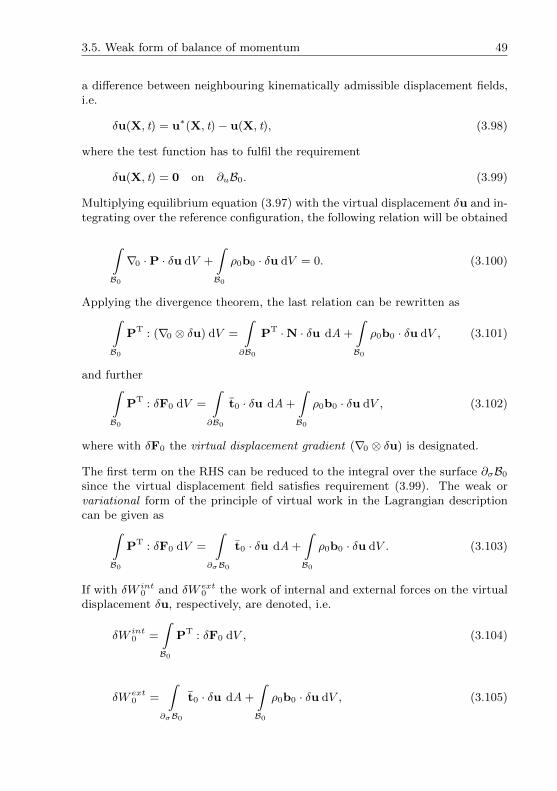
3.5. Weak form of balance of momentum 49
a difference between neighbouring kinematically admissible displacement fields,i.e.
δu(X, t) = u∗(X, t)− u(X, t), (3.98)
where the test function has to fulfil the requirement
δu(X, t) = 0 on ∂uB0. (3.99)
Multiplying equilibrium equation (3.97) with the virtual displacement δu and in-tegrating over the reference configuration, the following relation will be obtained
∫B0
∇0 ·P · δu dV +
∫B0
ρ0b0 · δu dV = 0. (3.100)
Applying the divergence theorem, the last relation can be rewritten as∫B0
PT : (∇0 ⊗ δu) dV =
∫∂B0
PT ·N · δu dA +
∫B0
ρ0b0 · δu dV , (3.101)
and further∫B0
PT : δF0 dV =
∫∂B0
t0 · δu dA +
∫B0
ρ0b0 · δu dV , (3.102)
where with δF0 the virtual displacement gradient (∇0 ⊗ δu) is designated.
The first term on the RHS can be reduced to the integral over the surface ∂σB0
since the virtual displacement field satisfies requirement (3.99). The weak orvariational form of the principle of virtual work in the Lagrangian descriptioncan be given as∫
B0
PT : δF0 dV =
∫∂σB0
t0 · δu dA +
∫B0
ρ0b0 · δu dV . (3.103)
If with δW int0 and δW ext
0 the work of internal and external forces on the virtualdisplacement δu, respectively, are denoted, i.e.
δW int0 =
∫B0
PT : δF0 dV , (3.104)
δW ext0 =
∫∂σB0
t0 · δu dA +
∫B0
ρ0b0 · δu dV , (3.105)

50 Chapter 3. Conservation equations and stress measures
the principle of virtual work, defined in the reference configuration, can be writ-ten in short form as
δW int0 = δW ext
0 . (3.106)
The same procedure can be applied to obtain the weak formulation of the prin-ciple of virtual work in an Eulerian description.
The Eulerian gradient of the virtual displacement is defined as
δF = δF0 · F−1 or ∇⊗ δu = (∇0 ⊗ δu) · F−1. (3.107)
Applying the last relation, (3.31), (3.29), (2.20) and (2.21) into Lagrangian form(3.103) the Eulerian form of the principle of virtual work will be obtained as∫
Bt
σ : (∇⊗ δu) dv =
∫∂σBt
t · δu da +
∫Bt
ρb · δu dv, (3.108)
with the traction boundary conditions defined on ∂σBt
σ · n = t (3.109)
and displacement boundary conditions defined on ∂uBt
u = u. (3.110)
3.5.2 Rate of the weak form of balance of momentum
Many numerical solution schemes for quasi-static elastoplastic problems performthe incremental solution based on the rate formulation of the weak form of thebalance of momentum. In the finite element formulation it leads to the contin-uum tangent stiffness matrix (cf. Simo & Hughes, 1998). Therefore, the rate ofthe weak form of equilibrium equation will be introduced here.
Instead of the virtual displacement field δu a kinematically admissible spatialvirtual velocity field δv may be introduced. The test function δv in any con-figuration Bt satisfies the requirement to vanish on ∂vBt and is tangent to thedeformation ϕ. Its corresponding quantity in the Lagrangian configuration isdenoted by δv0(X, t).
The material time derivative of equilibrium equation (3.97) defined in terms ofthe Lagrangian quantities is
∇0 · P + ρ0b0 = 0. (3.111)
Multiplying the last equation by the virtual velocity δv0, integrating over the ref-erence configuration and applying the divergence theorem, the rate-incremental

3.5. Weak form of balance of momentum 51
version of the Lagrangian weak form of the balance of momentum will be ob-tained as∫
B0
PT : (∇0 ⊗ δv0) dV =
∫∂σB0
˙t0 · δv0 dA +
∫B0
ρ0b0 · δv0 dV . (3.112)
Similarly as in (3.107) the spatial and referential gradient of virtual velocity arerelated as
∇⊗ δv = (∇0 ⊗ δv0) · F−1. (3.113)
Using (3.35), (2.45), (3.39), (3.58) and the last relation the virtual power densityof the LHS of equation (3.112) can be rewritten as
PT : (∇0 ⊗ δv0) = (L · τ +τ L) : (∇0 ⊗ δv0) · F−1
= (L · τ +τ L) : (∇⊗ δv).
(3.114)
Applying the last relation, (2.20) and (2.21) to the Lagrangian rate form therate of the Eulerian weak form of the balance of momentum can be written as∫
Bt
J−1(L · τ +τ L) : (∇⊗ δv) dv =
∫∂σBt
˙t · δv da +
∫Bt
ρb · δv dv, (3.115)
or, inserting the logarithmic objective rate instead of the Lie derivative of theKirchhoff stress according to (3.74),∫
Bt
J−1(L · τ +τ Log + ΥLog · τ − τ ·ΥLog−D · τ − τ ·D) : (∇⊗ δv) dv =
∫∂σBt
˙t · δv da +
∫Bt
ρb · δv dv. (3.116)

4 Constitutive relations
4.1 Introduction
In Chapter 3 the general principles, that determine the relation between ap-plied forces and the motion of the body of interest, were derived independentlyfrom the properties of the material the body is made of. On the other side, thestresses inside the body are the reactions of the deformation of material underconsideration induced by the external forces, thus, they are dependent of thematerial properties. Therefore it is necessary to express the stresses in termsof deformation measures, such as strain is. The group of laws that describethe relationship between the deformation measure and the stress measure, orbetween their rates, in continuum mechanics are termed constitutive equations.They obviously depend on the type of material and have to stay invariant withrespect to the change of frame since the material properties are independent ofthe frame of reference.
The aim of this Chapter is to provide the constitutive relations that can modeland predict the complex behaviour of materials under elastoplastic deformations,especially if they are large. The phenomenological aspect in developing the con-stitutive relations rather than the physically motivated approach of elastoplas-ticity is adopted here.
Elastoplasticity in general is a single entity that represents a complicated combi-nation of two totally different kinds of idealized material behaviour; pure elastic-ity and pure plasticity. The pure elastic process implies that during deformationthe whole work done is stored in the body as the internal energy and will becompletely recovered during the unloading process. That is why the pure elasticprocess is assumed as reversible and dissipationless. On the other side, the plas-tic deformation of material stands for irreversible and dissipative process whichimplies the permanent change in the shape and usually in the volume of the bodyof interest that cannot be recovered after the removal of the external agencies.
Elastoplastic processes are dependent of the loading history and deformation andstress states in the body will be described by the time-dependent tensor fields.Therefore the best way to model the elastoplastic behaviour of materials wouldbe by an incremental or rate type formulation, i.e. to give the relationship be-tween instantaneous elastic and plastic deformation increments (rates) and theinstantaneous stress increment (rate). The incremental essence of elastoplasticdeformation is a common base for both elastoplastic rate formulation and its
52

4.2. Continuum thermodynamics 53
finite element implementation.
The influences of the micro-mechanical processes in the material in the course ofelastoplastic deformations to the behaviour of the body on the macroscopic level,such as hardening effect occurrence, in phenomenological model are representedby the set of internal variables, for which the appropriate governing equationshave been developed individually.
In order to provide physically consistent prediction of the material behaviourthe thermodynamic laws are implemented. The introduced constitutive modelsare restricted to the isothermal, quasi-static and rate-independent processes.
4.2 Continuum thermodynamics
Elastoplastic deformations, whether they are small or finite, are by their na-ture partially reversible and partially irreversible processes. During the irre-versible process, usually addressed to plasticity, the dissipation of mechanicalwork occurs. The last conclusion is valid even for isothermal processes, whichwill be assumed here. During elastoplastic deformation only mechanical workand heat are assumed to be the sources of energy, i.e. any other influence on thedeformable body, such as chemical, electrical or magnetic, has been neglected.Thus, the elastoplastic deformations of the solid bodies can be treated as thermo-mechanical processes.
Our goal is to develop physically consistent material laws of finite elastoplas-ticity. Therefore, the kinematics and kinetics principles of a deformable body,presented in preceding Chapters 2 and 3, have to be strongly coupled with ther-modynamic principles (see Lehmann, 1989). Later on, when we restrict ourattention to the purely mechanical theory of elastoplasticity, any temperatureeffects will be ignored.
Within the concept of thermodynamics, the body of interest B, introduced inSection 2.2.1, geometrically occupies the region in space known as a control vol-ume. The region outside the control volume represents the environment withwhich the body B thermodynamically correlates. The control volume will beconsidered as a closed thermodynamic system for which the energy exchangewith the surrounding will be allowed while no matter exchange between thebody and the environment is permitted.
In Lehmann (1989), and the same will be adopted here, the basic assumptionsare the following: ”the body can be considered as a classical continuum”, i.e.the kinematics of the body of interest is defined according to the descriptiongiven in Chapter 2, and ” the thermodynamical state of each material element isdetermined uniquely by the actual values of a set of external and internal statevariables even if the body is not in thermodynamical equilibrium.” The mechan-

54 Chapter 4. Constitutive relations
ical state variables can describe the mechanical features of the body, for exampleits position in space or velocity, while the thermodynamical state variables, suchas density, temperature or stress, have to describe the thermodynamical state ofthe control volume. The change of the thermodynamic system state from its ini-tial state B0 to the actual state Bt is determined by the interaction between thethermodynamic system and its environment. This change represents a thermody-namic process which implies the change of the magnitudes of the state variablesas well. If the initial state of the system can be recovered by some additionalprocesses we can say that thermodynamic process is reversible. Otherwise, thethermodynamic process is assumed to be irreversible and it is characterised bythe significant change in the environment. In nature the irreversible processesare predominant.
Another idealisation adopted here will be that the process of deformation is veryslow, i.e. the rate of deformation is very low, in such a way that the subsequentinternal equilibrium state in the body can be reached faster than the externalprocess is processed. Therefore, the external process can be assumed as quasi-static. The reversible processes must be quasi-static while the opposite is notnecessary to be the case.
Also, we will assume that the temperature changes in the system occur slowlyenough that the system can continually adjust to the constant temperaturethrough the heat exchange with the environment. Likewise, the body B willnot be exposed to any exterior thermal influence. That means that only isother-mal processes are to be considered here which means that the temperature ofthe body is held constant, and independent of the particle spatial position andtime, but the thermal exchange between the thermodynamic system and its en-vironment still exists.
The state variables evolutions, whether these variables are tensors or scalars,have to be governed by the appropriate differential equations. Knowing the cur-rent values of the state variables provides that the current stress state of thebody of interest is determined without knowledge of the history of the processthat precede the current state of the deformable body. Regarding the implemen-tation of the developed phenomenological model in finite element procedure alimited number of internal variables, accompanied with their appropriate evolu-tion equations, have been adopted here.
4.2.1 First law of thermodynamics
In a thermo-mechanical process, where only mechanical work and heat are as-sumed to be the sources of energy, the first law of thermodynamics plays a crucialrole. That means that the thermodynamic process in material body implies thestrong coupling between deformation and heat, i.e. that is the process in whichthe mechanical work and the heat are constantly converted into each other.

4.2. Continuum thermodynamics 55
Developing the first law of thermodynamics we will consider arbitrary thermo-dynamic processes firstly and later on we will confine ourselves to the restrictedthermo-mechanical processes. For arbitrary thermodynamic process, the sum ofthe work rate of the applied forces and the rate of the heat supplied to the bodyequals the rate of the total energy of the body, i.e. the rate of the kinetic andthe internal energy of the body. Shortly, the rate form of the balance of energycan be written as
Wext
+ Q = Wkin
+ U . (4.1)
In the last relation, the rate of the heat supplied to the body is determined by
Q =
∫∂Bt
−q · n da +
∫Bt
rρ dv =
∫Bt
[−∇ · q + rρ] dv, (4.2)
where the heat transfer across the boundaries of the body is determined by heatflux vector q(x, t) while the heat generated within the body is defined by heatsource r(x, t). Since the positive flux is directed out of the body the heat fluxterm in the last relation has to be of the negative sign if the heat is added tothe body, and the opposite. In the last relation the divergence theorem has beenapplied.
We can now recall Eq. (3.45)
Wext
=
∫Bt
ρb · v dv +
∫∂Bt
t · v da, (4.3)
and define the kinetic energy rate in the same manner as in Section 3.3.3 as
Wkin
=d
dt
∫Bt
1
2ρv · v dv. (4.4)
If the internal energy U of the body B will be represented by a specific internalenergy u, the rate of internal energy can be defined as
U =
∫Bt
u ρ dv. (4.5)
Introducing Eqs. (4.3), (4.2), (4.4) and (4.5), respectively, into (4.1), the follow-ing relation will be obtained∫
Bt
ρb · v dv +
∫∂Bt
t · v da +
∫Bt
[−∇ · q + rρ] dv
=d
dt
∫Bt
1
2ρv · v dv +
∫Bt
u ρ dv, (4.6)

56 Chapter 4. Constitutive relations
which represents a global form of the total energy balance for an arbitrary ther-modynamic process.
Since the rate of work of the applied forces can be presented as (3.48), i.e. thefirst two terms in the last equation can be replaced with the RHS of Eq. (3.48),we can conclude that the rate of internal energy is given as∫
Bt
u ρ dv =
∫Bt
tr (σ ·D) dv +
∫Bt
[−∇ · q + rρ] dv, (4.7)
that is∫Bt
u ρ dv =
∫Bt
[tr (σ ·D)−∇ · q + rρ] dv. (4.8)
The last relation represents the global form of the balance of internal energy ofthe body. From relation (4.7) comes that the rate of internal energy is equal tothe sum of the rate of internal work, defined by Eq. (3.51), and the rate of theheat supplied to the body, i.e.
U = Wint
+ Q. (4.9)
Since relation (4.8) is valid for any subdomain of Bt, the corresponding localform of the balance of internal energy can be written as
u ρ = tr (σ ·D)−∇ · q + rρ. (4.10)
Eq. (4.10) states that the local form of the first law of thermodynamics, forarbitrary thermodynamic process, represents the sum of the internal stress powerper current unit volume (defined earlier by Eq. (3.52)) and the internal non-mechanical power per current unit volume due to the heat flux and heat sources,i.e.
u ρ = w −∇ · q + rρ. (4.11)
As it has already been mentioned, we are focused only on the pure mechanicalisothermal processes where no additional heat has been given to the body orremoved from it neither through the boundary nor through the volume of thesystem. The only heat producer is the body itself due to the micro-mechanicalchanges in the structure of the body during the irreversible plastic deformation,which causes internal dissipative processes. The source of this part of conductedheat is hidden in the stress power. According to Lehmann (1982), the stresspower can be decomposed into three parts: wr that is reversible in strict sense,wd that is dissipated immediately, and the third, wh, which represents the storedmechanical energy due to the changes of the internal structure of the material.The local form of the balance of internal energy is then given as
u ρ = w = wr + wd + wh. (4.12)

4.2. Continuum thermodynamics 57
That means that during the isothermal and quasi-static process the specificinternal energy will be changed only due to the change of the stress power andthe latter depends on the internal processes in the body. Globally, it means thatthe rate of internal energy of the body will be equal to the rate of internal workor, according to (3.49), the global form of the first law of thermodynamics forisothermal and quasi-static processes yields to
U = Wint
= Wext
. (4.13)
That means that, neglecting all external thermal effects, the whole work pro-duced by the external forces will be used for increasing the internal energy ofthe deformable body, which later can be partially dissipated and partially not.
4.2.2 Second law of thermodynamics and principle of maximumdissipation
The first law of thermodynamics defines the energy balance of the deformablebody, but it cannot describe macroscopic irreversible effects of thermodynamicprocesses due to some microscopic occurrences, such as the local rearrangementsof microstructure caused by elastoplastic deformations. It is also well known thatheat can be transferred only from wormer to colder body. Likewise, mechanicalwork can be converted into heat but the opposite process is possible only underspecial circumstances and with not so high coefficient of utilization. For thedescription of these phenomena the second law of thermodynamics has to beintroduced. The latter defines the possible directions of the energy exchangeand some restrictions of the observed thermodynamic process as well.
We will again start from an arbitrary thermodynamic process. As a measureof a microstructural disorder of the system and a total local dissipation of thethermodynamic process a scalar quantity named entropy S has been introduced.Its rate of change can be defined as
S ≥∫∂Bt
−q · nθ
da +
∫Bt
r
θρ dv, (4.14)
which represents the global form of the Clausius-Duhem inequality, where withθ the absolute (local) temperature has been designated.
For pure reversible processes the following relation holds
Srev
=
∫∂Bt
−q · nθ
da +
∫Bt
r
θρ dv, (4.15)
which demands the existence of the irreversible part of the rate of entropy, too,for arbitrary reversible-irreversible process such as elastoplastic deformation, i.e.

58 Chapter 4. Constitutive relations
Sirr
= S − Srev ≥ 0. (4.16)
The reversible part of the rate of entropy Srev
can be exchanged with the enviro-
ment through the boundaries while the other part Sirr
represents the productionof the entropy inside of the body due to the irreversible process. Therefore, theglobal form of the balance of entropy, for an arbitrary thermodynamic process isgiven as
S = Srev
+ Sirr
, (4.17)
i.e. ∫Bt
sρ dv =
∫Bt
[−∇ ·
(q
θ
)+r
θρ+ sirrρ
]dv, (4.18)
where with s and sirr specific entropy and specific irreversible entropy per currentunit volume have been designated, respectively. In the local form, the balanceof entropy can be presented as
sρ = −∇ ·(
q
θ
)+r
θρ+ sirrρ. (4.19)
Expanding the term ∇ · (q/θ) and applying the first law of thermodynamics forarbitrary thermodynamic process (4.11), the following equation will be obtained
θsρ =1
θq · ∇θ + uρ− w + θsirrρ. (4.20)
Since sirr physically represents the local dissipation, and therefore it is alwaysgreater than or equal to zero, the dissipation function D will be introduced as
D = θsirrρ ≥ 0. (4.21)
In the last relation a zeroth law of thermodynamics has been applied, too, i.e.it is assumed the absolute temperature is θ ≥ 0. Thus, comparing the last tworelations, the following conclusion can be made
D = w − uρ+ θsρ− 1
θq · ∇θ ≥ 0. (4.22)
According to Truesdell & Noll (2004), the dissipation function can be split intomechanical and thermal part as
D = Dmech +Dth ≥ 0, (4.23)

4.2. Continuum thermodynamics 59
where
Dmech = w − uρ+ θsρ ≥ 0, (4.24)
and
Dth =1
θq · ∇θ ≥ 0. (4.25)
To represent a thermodynamic potential that measures the work that can beused from a closed thermodynamic system, the specific Helmholtz free energy ψper unit reference volume, defined as
ψ = u− θ s, (4.26)
will be introduced now.
The rate of the specific Helmholtz free energy will be defined as
ψ = u− θ s− θs, (4.27)
and for the arbitrary thermodynamic process, the rate of the specific Helmholtzfree energy per unit current volume is
ψρ = uρ− θ sρ− θsρ. (4.28)
The last relation can be rewritten as
θsρ = uρ− θ sρ− ψρ, (4.29)
If the last relation is introduced in Eq. (4.24), the definition of mechanicaldissipation in terms of Helmholtz free energy of the arbitrary thermodynamicprocess is obtained as
Dmech = w − θ sρ− ψρ. (4.30)
For adopted isothermal processes, where θ = 0, the last relation yields
Dmech = w − ψρ = σ : D− ψρ ≥ 0, (4.31)
per unit current volume, or per unit reference volume
Dmech = τ : D− ψ ≥ 0. (4.32)
The classical rate-independent plasticity model can be obtained by postulatingthe last relation that stands for the local principle of maximum dissipation (cf.Simo & Hughes, 1998). Our goal would be to define the actual state of thesystem, i.e. to determine the actual values of the stress and the adopted internalvariables among all admissible states of stress and internal variables for whichthe plastic dissipation, or Dmech, attains a maximum.

60 Chapter 4. Constitutive relations
Since our concern is the purely mechanical theory of elastoplasticity we willbe interested in the first term of the dissipation inequality (4.32), i.e. in thestress power, only. The further elaboration of this topic from a general point ofview will be excluded here. For our further research the main interest is in theconsequences of the aforestated principle of maximum dissipation, and they willbe given in Section 4.5, while the exact derivation of the constitutive relationwith the principle of maximum dissipation as a starting point would be omittedhere. For more details the reader is referred to the following references that aredealing with this problematic Lehmann (1982), Simo (1988), Lehmann (1989),Pohe & Bruhns (1993), Lubarda (2001), Xiao et al. (2007), Luig (2008), Bertram(2012).
In this treatise, in developing the constitutive relations as a starting point willbe used the work postulate and this topic will be elaborated in Section 4.5.
4.3 Decomposition of the stress power
Even though the balance of mechanical energy developed in Section 3.3.3 doesnot exist in reality, because each process has some thermal dissipation, accordingto the assumptions specified in Section 4.2, the first law of thermodynamics foradopted isothermal and quasi-static process (4.12) should be assumed as valid.It states that the increment of the specific internal energy is equal to the stresspower, i.e.
u ρ = w = wr + wd + wh. (4.33)
For a purely elastic deformation, the energy produced by external forces willcause the increase of internal energy of the body that will be stored as theelastic internal energy and is fully recoverable during the process of unloading.In that case the total stress power w will be identical to its reversible or re-coverable part wr. On the other side, during the elastoplastic deformation theinternal energy will be partially recovered and partially dissipated. According toLehmann (1989), in general, alongside the recoverable part of the stress powerwr addressed to elastic deformation, the inelastic or irrecoverable part of thestress power, addressed here to plastic deformation, will occur and it will notdissipated totally. One part wd dissipates immediately while the second partwh ”is stored in the micro-stress fields generated by lattice defects (leading to ahardening of the material)”. That leads us to the conclusion that the total stresspower w is composed of a recoverable part and an irrecoverable part during everyprocess of elastoplastic deformation. If with we = wr and wp = wd + wh therecoverable (elastic) and irrecoverable (plastic) part of the total stress power perunit reference volume are designated, respectively, the work conjugacy relation(3.75) can be rewritten as
w = τ : D = we + wp. (4.34)

4.4. Hypo-elasticity 61
For large elastoplastic deformations, applying the additive decomposition of anEulerian rate of deformation tensor D given by (2.109), the stress power partscan be defined as
we = τ : De and wp = τ : Dp. (4.35)
To ensure that this separation is consistent with the physical background of it,the constitutive formulations for De and Dp should be established in such a waythat De is indeed elastic-like (recoverable), while Dp is plastic-like (dissipative).
4.4 Hypo-elasticity
4.4.1 Hypo-elastic relation for De - From small to finite strains
The elastic behaviour at small deformations may be described by the generalizedHooke’s law. Its rate form may be given by
εe =1 + ν
Eσ − ν
E(tr (σ))1, (4.36)
where with ν and E the material constants Poisson’s ratio and Young’s moduluswere designated while 1 represents the unit second-order tensor.
The last relation can be applied to the case of finite deformations as well bysimply replacing the elastic strain rate εe with the elastic stretching De. As ithas already been shown, the material time derivative of an Eulerian stress tensoris not an objective quantity. Therefore the material time derivative in Euleriandescription has to be replaced by an objective rate. Constitutive equations haveto be consistent with thermodynamics, i.e. the stress and strain measures haveto be the work-conjugated pairs. Thus, we will choose, instead of the Cauchystress, the Kirchhoff stress in conjunction with an Eulerian Hencky strain.
Finally, the objective extension of Eq. (4.36) for the case of finite deformationmay be given as
De =1 + ν
E
τ − ν
E(tr(τ)
)1. (4.37)
The last relations represents a hypo-elasticity model of grade zero. It is thesimplest form of the general hypo-elasticity model
De = H(τ ) :τ , (4.38)
at first introduced by Truesdell (cf. Truesdell, 1955a, 1955b, 1956). Here, H(τ ) isthe fourth-order stress-dependent moduli named hypo-elasticity tensor, which inorder to fulfil the requirement of material frame-indifference has to be isotropicwith respect to τ ( cf. Xiao et al., 1997a).

62 Chapter 4. Constitutive relations
In developing the hypo-elastic constitutive relation the most important step isa proper choice of the corotational rate type implemented in the previous rela-tions.
The first proposed and widely used objective rate was the corotational Jau-mann rate. It is also implemented in all commercial codes for finite deformationcalculations. However, in the studies of Lehmann (1972), Dienes (1979) andNagtegaal & de Jong (1982) it was shown that the hypo-elasticity model basedon the Jaumann rate gives an unstable response at simple shear, known as shearoscillatory phenomenon, and that for the case of large rotation the Jaumannrate is an inappropriate choice.
The aforementioned facts motivated the developing and application of severaldifferent objective rates, corotational and non-corotational, such as the Trues-dell rate, the Green-Naghdi rate, the Cotter-Rivlin rate, the Durban-Baruchrate, etc. (see Sections 2.6.4 and 2.6.5 and references therein for details).
Simo and Pister (cf. Simo & Pister, 1984) have elucidated that for the case ofpure elastic deformation, where D = De and when the recoverable elastic-likebehaviour is expected, none of the constitutive hypo-elastic relations, based onthe at that time known objective rates, san fulfil the integrability condition togive an elastic relation, i.e. the path-dependent and dissipative processes havebeen detected for all rates.
Kojic & Bathe (1987) have also shown that application of the Jaumann stressrate produces residual stresses at the end of an elastic closed strain path. Thistopic will be discussed in detail in Section 5.2.
All above stated were the reasons why the additive decomposition of the stretch-ing was treated as inappropriate starting point for finite elastic-plastic deforma-tion descriptions except for the case of metal plasticity where finite total butsmall elastic deformations occur. It was taught that the error in modelling theelastic deformation part by a hypo-elastic relation can be ignored since thatdeformation is small in comparison with the plastic deformation (cf. Simo &Hughes, 1998). Even though the intention of Truesdell was that hypo-elasticrate equation (4.38) described finite elastic deformation behaviour, the reliabil-ity of this relation stayed at that time at the level of small elastic deformations.
When the logarithmic rate was discovered by several researchers independently(cf. Lehmann et al., 1991; Reinhardt & Dubey, 1996; Xiao et al., 1997b, 1998a),the above stated problems have been solved by introducing the logarithmic ratein the hypo-elastic constitutive relation.
If in the general hypo-elastic relation (4.38) and in its simplest form of gradezero (4.37) the logarithmic rate is implemented, the following relations will be

4.4. Hypo-elasticity 63
obtained
De = H(τ ) :τ Log, (4.39)
and
De =1 + ν
E
τ Log − ν
E(tr(τ Log
))1, (4.40)
respectively.
According to Bruhns et al. (1999) and Xiao et al. (1999, 2000a), in order to bethe real constitutive equation of finite elasticity, Eq. (4.39) has to fulfil the so-called elastic integrability criterion, i.e. ”for every process of elastic deformationswith De = D, the rate equation (4.39) should be exactly integrable to delivera dissipationless elastic relation and hence really characterize recoverable elasticbehaviour”. This criterion will be fulfilled only if the objective rate in the samehypo-elastic relation is assumed to be the logarithmic rate. As a consequence,the simplified form of the hypo-elastic relation (4.40) will be exactly integratedto give a purely elastic relation; Cauchy elastic or Green elastic, if an appropri-ate potential exists, as it will be shown in the next Section. For integrabilityconditions relating hypo-elasticity to elasticity in Cauchy’s sense and in Green’ssense the reader is reffered to Xiao et al. (1997a).
Regardless to the strong influence of rotations, which usually has caused a lot ofproblems with other rates, the implementation of the Log-rate in the numericalcalculations gives the stable solution for finite simple shear and the dissipation-less responses for the elastic cyclic deformations. This statement will be provedwith the numerical results which will be shown in Section 5.2.3.
4.4.2 Hyper-elastic potential
For the group of hyper-elastic or Green-elastic materials holds that there existsa scalar elastic potential Σ as function of Lagrangian strain E and its derivativewith respect to the strain E is simply related with the Lagrangian stress T as
T =∂Σ
∂E. (4.41)
A similar relation can be written for the Eulerian quantities as well. If we wantthe true stress to be derived from the elastic potential then an elastic potentialW as a function of the Eulerian Hencky strain h has to be introduced. Forisotropic elastic materials the last relation can be written as
τ = Jσ =∂W
∂h, (4.42)

64 Chapter 4. Constitutive relations
where the elastic potential W is an isotropic function of h, i.e. W = W (h).There exists a complementary elastic potential W as function of the Kirchhoffstress, i.e. W = W (τ ), such that the Hencky strain is derived from
h =∂W
∂τ. (4.43)
These two elastic potentials satisfy the relation
W + W = τ : h. (4.44)
The second gradients of the elastic potential, ∂2W/∂h2, and complementaryelastic potential, ∂2W/∂τ 2, represent the elastic tangent stiffness and elastictangent compliance tensor, respectively. Replacing the hypo-elasticity tensorH by the elastic tangent compliance tensor, the hypo-elastic relation (4.38) forhyper-elastic materials will be given as
De =∂2W
∂τ 2:τ . (4.45)
With the logarithmic rate implementation in the last relation, the followinghypo-elastic relation will be obtained
De =∂2W
∂τ 2:τ Log, (4.46)
which can be exactly integrated to give the hyper-elastic relation
h =∂W
∂τ. (4.47)
For the simplest form of the complementary potential W given by an isotropicquadratic function, the second gradient of the complementary elastic potentialresults in a constant and isotropic instantaneous elastic compliance tensor KKK
KKK = CCC−1 =1 + ν
EIII− ν
E1⊗ 1, (4.48)
where with CCC the instantaneous elasticity tensor has been designated. Tensor CCCis also constant and isotropic tensor which represents the second gradient of theelastic potential W . With III and 1 the symmetric fourth-order and the second-order unit tensors, respectively, have been introduced.
The hypo-elastic relation (4.45) than will be given in the form
De = KKK :τ =
1 + ν
E
τ − ν
E(tr(τ)
)1. (4.49)
That means that over the infinitesimal time interval (t, t + dt), from Eq. (4.49)the relation between the instantaneous elastic strain increment De dt and the

4.5. Plasticity 65
instantaneous stress incrementτ dt can be established via the instantaneous
elastic compliance tensor KKK, where the latter will be constant over the wholeintegration elastic range. The last statement is very important for further nu-merical implementation of the constitutive law of elasticity using the hypo-elasticformulation.
The last relation can be written in its inverse form as
τ = CCC : De, (4.50)
or in terms of Lame elastic constants λ and µ,
τ = λtr
(De)1 + 2µDe, (4.51)
where, for the given Young’s modulus and Poisson’s ratio, the first Lame constantλ and the second Lame constant µ can be obtained by the following relations
λ =Eν
(1 + ν)(1− 2ν)and µ =
E
2(1 + ν). (4.52)
With a use of the logarithmic stress rate, Eqs. (4.50) and (4.51) are given,respectively, as
τ Log = CCC : De and
τ Log = λtr
(De)1 + 2µDe. (4.53)
By an integration of equation (4.53)2 the isotropic elastic relation will be ob-tained as
τ = λln(detV)1 + 2µlnV, (4.54)
where V is the left stretch tensor defined in Section 2.3.2 and, according to(2.39), lnV = h.
The above given isotropic elastic relation (4.54) is the natural generalization ofthe small deformation Hooke’s law where the infinitesimal strain is replaced bythe Hencky strain. In a study by Anand (1979, 1986) it has been shown thatthis elastic relation is in a good agreement with experiments for a wide class ofmaterials for moderately large deformations.
For comprehensive derivations and explanations see Xiao et al. (2006a) andreferences cited above.
4.5 Plasticity
If the deformation of the body of interest is increased beyond a certain limitso that it cannot be fully recovered during the unloading process, the residualdeformations will stay locked in the body and the material starts to plastify. The

66 Chapter 4. Constitutive relations
constitutive relations, derived in the last Section, are no longer valid in the areaswhere the plastification occurs and a new relationship between stress and strainhas to be defined. Defining the constitutive relation in the field of plastic defor-mations is a more complex process because plastic deformations do not dependonly on the stress but also on the whole history of the process. Regarding the laststatement, constitutive relations of plasticity are generally developed in terms ofstrain increment (rate) and stress increment (rate). Additionally, according tothe adopted approach presented in Section 4.2, the set of internal variables haveto be introduced and their evolution equations have to be governed to ensurethe correct determination of the current deformation state of the body.
Two approaches in developing the constitutive relations of rate-independentelastoplasticity have been considered in this treatise. The first is based on theprinciple of maximum plastic dissipation derived from the second law of ther-modynamics, which is introduced in Section 4.2.2, while the second relies onthe work postulate, which is also expressed in terms of the universal stress workconcept in thermodynamics. The first one is more general and more physicallyconsistent, while the second is more practical and simplified. In the second ap-proach Drucker’s postulate and Ilyushin’s postulate play a fundamental role.
Our main achievement would be to obtain the results that are consistent withthe experimental results, and that would be possible by any of aforestated ap-proaches if a special care is taken about the physical nature of the examineddeformation process. Even though the first approach is more general, at somelevel some assumptions or idealisations have to be introduced. That demandsa deep understanding of the problem in order to develop the correct theoreticalbase whose further task will be to produce the accurate results that will stay inthe frame of theoretically and experimentally expected. On the other side, ”evenit is not a universal principle in a general sense, the work postulate expressesa common physical essence only for a class of typical elastoplastic materials in-cluding metals and alloys etc. However, this class of typical materials is alreadybroad enough and usually just the main concern or object in the development ofelastoplastic theory. Thus, it might be desirable that a reasonable constitutivetheory for this large class of typical materials should be endowed with a structureas simple as possible.” Also, ”here, our concern is with the purely mechanicaltheory of elastoplasticity without pronounced temperature effects. In this case,the aforementioned work postulate may play a role as quasi-thermomechanicalfoundation for the class of typical elastoplastic materials. No attempt beyondthis will be pursued” (Xiao et al., 2006a).
The main reason for adopting the work postulate based approach rather thanthe maximum plastic dissipation is in our intention to develop the constitu-tive relations that are as simple as possible but reliable in prediction of the finiteelastoplastic material behaviour for the target group of materials, such as metals

4.5. Plasticity 67
and alloys. In numerical finite element calculations the integration of elastoplas-tic rate constitutive equations will be called for in every process of numericaliteration at each time step and for each element. That results into the fact thatthe numerical calculation could be time consuming and very cumbersome if theconstitutive relations involved additional variables and their evolution equationsas well, especially if the more demanding engineering model had to be solved.
Of course, if we want to introduce the more complex material model or if sig-nificant thermal effects have to be taken into account, where the temperaturebecomes one of the important state variables, the use of the work postulate hasto be re-examined.
4.5.1 Yield surface and loading condition
That behaviour of materials in the plastic region is observed as a history depen-dent process bounded by a yield condition, which for small deformations can berepresented in the following form:
F (σ, εp, k(εp)) = 0, (4.55)
if isothermal processes are taken into account. In the last relation, the scalar k,known as the hardening variable, takes into acount the history of deformation.According to Hill (1950), it can be represented by the accumulated plastic work
k1 = wp =
t∫0
σ : εp dt, (4.56)
or the equivalent or effective plastic strain
k2 = εpeqv =
t∫0
(2
3εp : εp)
12 dt. (4.57)
In this treatise the first approach will be adopted.
In the stress space, the function F , given by (4.55), represents the surface thatis surrounding the origin, where σ = 0, and the elastic range (see Fig. 4.1a).Usually, the function F is termed as a loading function and F0 is an initial yieldfunction while their corresponding surfaces in the stress space are the loadingsurface and yield surface, respectively. For metals, due to the hardening, theyield surface will expand, translate and distort in stress space. Therefore, rela-tion (4.55) represents a family of yield surfaces. In Figure 4.1a, with F = F1 andF = F2 the subsequent yield surfaces have been presented. For some materials,such as concrete and soil, the opposite behaviour has been observed, i.e. theyield surface contracts in the stress space due to softening phenomena.

68 Chapter 4. Constitutive relations
Figure 4.1: Initial and succeeding yield surfaces and material stability
Figure 4.2: Loading condition, normality rule and convexity of the yield surface
If the stress changes the loading function will change as well. From Eq. (4.55)it will be obtained
dF =∂F
∂σ: dσ +
(∂F
∂εp+∂F
∂k
∂k
∂εp
): dεp. (4.58)
As a result of the change of the loading function, three different cases are possi-ble.
If dF > 0, in the observed point of the deformable body the angle between thedirection of the stress increment dσ1 and the direction of the gradient of theloading surface (or of possible direction of plastic deformation dεp as it will beshown later) is smaller than 90 (see Figure 4.2). This case corresponds to theloading process and plastic behaviour of material in the observed point.
The second case, when dF = 0 and the plastic deformation is not increasing

4.5. Plasticity 69
while the stress is changing, is characterised as a neutral loading. The direction
of the stress increment dσ2 is orthogonal to∂F
∂σ.
The case when dF < 0 corresponds to the unloading process, dεp = 0 and mate-rial behaves elastically. The angle between the direction of the stress incrementdσ3 and the direction of the gradient of the loading surface is now grater than90.
Mathematically these cases can be described as
∂F
∂σ: dσ1 > 0 (plastic behaviour)
∂F
∂σ: dσ2 = 0 (neutral process)
∂F
∂σ: dσ3 < 0 (elastic behaviour).
(4.59)
Thus, it can be concluded that for the materials which harden, two conditionshave to be satisfied for the onset of plastic deformations. The first requirementis that the stress has to reach a threshold value on the yield surface specific forthe observed material. The second requirement is that certain loading directionis required, described by the following loading condition
LC =∂F
∂σ: dσ1 > 0. (4.60)
4.5.2 Priniple of maximum plastic dissipation and its consequences
As it has been already mentioned, during the elastoplastic deformation the storedinternal energy will be partially recovered and partially dissipated in the unload-ing process, i.e. the total stress power per unit volume w consists of a recoverablepart and an irrecoverable part during every process of elastoplastic deformation.For small deformations the irreversible plastic mechanical work rate is definedas
wp = σ : εp. (4.61)
Generalising the relations valid for the one-dimensional tensile test for hardeningmaterials, e.g. presented in Figure 4.1b, Drucker has defined the stable or work-hardening materials. This definition is known as a Drucker’s postulate and statesthat stable materials are those in which additional stresses produce nonnegativework during a loading process and the work done by the additional stresses inthe loading-unloading cycle is positive if plastic strains occur, or equal zero whenthe strains are purely elastic. These definitions can mathematically be presented

70 Chapter 4. Constitutive relations
as
dσ : dε ≥ 0,∮(σ − σ∗) : dε ≥ 0.
(4.62)
Let us consider the material has already been loaded above the initial yieldlimit. In the last relation, (4.62)2, σ∗ is an arbitrary starting point in stressspace which is in the current elastic range (point A in Figures 4.1a and 4.1b).Induced by the external agency the stress is increasing to the value σ that reachesthe current yield surface F = F1 (point B in the Figures). The additional stressincrement dσ will produce the additional plastic deformation during the loadingprocess (point C in the Figures) and cause the expanding of the yield surfaceto the succeeding level F = F2, or stay on the current yield surface during aneutral process (point B′ in Figure 4.1a). The process of unloading from pointC to the initial stress value σ∗ (point D in Figure 4.1b and A in 4.1a) closesthe deformation cycle. It can be observed from Figure 4.1b that during thisdeformation the remained plastic strain dεp will occure at the end of the cycle.
Since the elastic strains are completely reversible and independent of the loading-unloading path, i.e.∮
(σ − σ∗) : dεe = 0, (4.63)
for the arbitrary closed path ABCD it comes∮(σ − σ∗) : dεp ≥ 0. (4.64)
Since the point A is arbitrarily chosen, inequality (4.62)2 will be satisfied if theintegrand of the last integral is nonzero. Finally, the following inequalities arerepresenting Drucker’s postulate
(σ − σ∗) : dεp ≥ 0,
dσ : dεp ≥ 0.(4.65)
Drucker’s postulate consequently implies
(σ − σ∗) : εp ≥ 0. (4.66)
The last inequality is known as principle of maximum of plastic dissipation.
The plastic dissipation is defined as
Dp = σ : εp, (4.67)
(cf. Lubliner, 2008). When the stress σ is found inside the yield surface, thenthe plastic strain rate and thus the dissipation vanish. If the stress during the

4.5. Plasticity 71
loading process is found on the yield surface, according to the second law ofthermodynamics Dp ≥ 0. Relation (4.66) can now be rewritten as
Dp ≥ σ∗ : εp. (4.68)
As it was stated earlier in Section 4.2.2, the principle of maximum plastic dis-sipation characterises the actual stress state (accompained by the actual valuesof the state variables) as a state among all admissible states for which plasticdissipation attains a maximum (Simo & Hughes, 1998).
The consequences of this principle of maximum plastic dissipation are very im-portant in plasticity theory.
The first consequence is that the plastic strain increment in stress space is or-thogonal to the yield surface in any point of it. This condition is often calledthe normality rule and is defined as
εp = Λ∂F
∂σ, (4.69)
where Λ is a plastic multiplier greater than zero that will be determined later.
From the last equation it can be observed that the yield function F defines theyield surface but it can be understood as a plastic potential as well. In thiscase normality rule (4.69) is called a flow rule that is associated with the yieldcriterion or associated flow rule in the stress space. For some materials the flowrule has to be defined from a plastic potential that is different from the yieldfunction and it is then termed a non-associated flow rule.
The second consequence of the maximum plastic dissipation postulate is the con-vexity of the yield surface observed from the top of its outward normal vector.
The third consequence would be the loading conditions that are already elabo-rated in the previous Section.
For details the reader is reffered to more comprehensive texts such as Hill (1950),Lubliner (2008), Khan & Huang (1995), Simo & Hughes (1998), Lubarda (2001).
4.5.3 Eulerian description of finite plastic deformations
In this Section the constitutive relations for finite plasticity will be derived, basedon the approach proposed in the last Section for the small deformation case.
The general form of the yield condition in the Eulerian description can be pre-sented as
F (σ, θ,qn) = 0, (4.70)

72 Chapter 4. Constitutive relations
where σ is an appropriate Eulerian stress measure, θ is relative temperature andqn represents a set of internal variables. If we confine ourselves to isothermalprocesses and take into account that for metals the plastic behaviour of materialis usually independent of the hydrostatic stress, the yield condition can be givenby the von Mises yield function
F = (σ′ −α) : (σ′ −α)− g(κ). (4.71)
In the last relation, α and κ are a symmetric Eulerian second-order tensor anda scalar, respectively, representing internal variables. The former is named backstress and represents a midpoint coordinate of the yield surface while the lattercan be interpreted as a reduced accumulating plastic work. The back stresscorresponds to the kinematic hardening while the variable κ is characterizingthe isotropic hardening.
The stress deviator, used in the last equation, is determined by the followingrelation
σ′ = σ − 1
3tr (σ)1. (4.72)
The reason for using the stress deviator instead of the stress itself can be clarifiedwith the introduction of the so-called π plane. In the three-dimensional space ofprincipal stresses, the π plane is determined with a normal vector n inclined withequal angles to the coordinate axes. Since the yield surface does not depend onthe hydrostatic stress the surface can be described by the same shape in planeswith the given normal n. If the yield surface is forming the cilinder in the givencoordinate system, its projection in the π plane will be a circle. The newlyintroduced isotropic hardening function g(κ) in Eq. (4.71) describes the growthof the yield surface in the π plane, and it depends on the internal parameter κ.
In the Eulerian finite elastoplasticity description the Eulerian Hencky strain hand Kirchhoff stress τ will be chosen as appropriate variables since they form aunique Eulerian work conjugate pair satisfying the necessary requirements, as itwas pointed out in Section 3.4. Thus, relation (4.71) will become
F = (τ ′ −α) : (τ ′ −α)− g(κ). (4.73)
If with τ the shifted Kirchhoff stress has been designated and given as
τ = τ ′ −α, (4.74)
the final shortened form of the yield condition is
F = τ : τ − g(κ). (4.75)
The normality rule (4.69) for large plastic deformations can be shown as
Dp = Λ∂F
∂τ ′. (4.76)

4.5. Plasticity 73
To fulfill the yield condition, during plastic deformations the stress must stay atthe yield surface, i.e. the time derivative of the loading function must vanish
F = 0. (4.77)
The last relation represents the so-called consistency condition. The materialtime derivative of yield function (4.73) is
F =∂F
∂τ ′:τ ′ Log +
∂F
∂α:αLog +
∂F
∂κκ = 0. (4.78)
Here, the logarithmic rate has been introduced to fulfill the requirement of ob-jectivity. Moreover, it has been shown in Xiao et al. (2000a), that once theobjective rate has been fixed this choice must be kept to avoid inconsistencies.
The internal variables α and κ may be governed by the following evolutionequations
αLog = c (κ) Dp,
κ =1
2
∂F
∂τ ′: Dp = τ : Dp.
(4.79)
Based on the INTERATOM model (see Bruhns et al., 1988) the proposed rela-tions for the scalar functions g(κ) and c(κ) are of the forms
g(κ) = g0 + gs [1− exp (−c1κ)] ,
c(κ) = cs [1− exp (−c1κ)] .(4.80)
For the known material parameters, Young’s modulus E and Poisson’s ratio νas elastic parameters, and the yield stress σy and tangent modulus Et as plasticparameters, the unknown coefficients in Equations (4.80) can be determined by
g0 =2
3σ2y, gs =
2
3(σ2s − σ2
y), (4.81)
where g0 and (g0 + gs) represent the squares of the initial and saturated radii ofthe yield surface, respectively, and σs is the saturated stress obtained from theexperimental record of a uniaxial cyclic deformation process.
If a new material parameter B has been introduced and given as
B =Et
(1− EtE
), (4.82)
then
c1 =2B
gsand cs = B. (4.83)

74 Chapter 4. Constitutive relations
The proposed model describes a combined kinematic-isotropic hardening be-haviour of material. As the cyclic process proceeds, at the beginning, the modelshows a pronounced isotropic hardening behaviour of material, i.e. an expansionof the yield surface prevails. During the deformation process the kinematic hard-ening is starting to dominate, leading to a saturation of the stress-strain curve.This behaviour can be observed in cyclic tests for most metals and the proposedconstitutive model predicts the material behaviour which is in accordance withthat observed in experimental records. For the numerical results of the proposedmodel the reader is referred to Section 5.3.
The objective time derivative of the Kirchhoff stress deviator can be determinedas
τ ′ Log = CCC :
D− τ τ : CCC : D
g(κ)
[c(κ) + 1
2
∂g(κ)
∂κ
]+ τ : CCC : τ
, (4.84)
where CCC is the instantaneous elastic stiffness tensor and D is the stretching ten-sor.
From the consistency condition (4.78), using (4.76) and (4.79), the plastic mul-tiplier Λ can be established as
Λ =τ :
τ ′ Log
2g(κ)
[c(κ) + 1
2
∂g(κ)
∂κ
] . (4.85)
Introducing Λ in (4.76) will give the final form of the normality rule for finiteplastic deformations
Dp = Λ∂F
∂τ ′= ρ
τ :τ ′ Log
2g(κ)
[c(κ) + 1
2
∂g(κ)
∂κ
] τ , (4.86)
where ρ is the loading-unloading factor, taking the values
ρ =
0 if F < 0 or F = 0 and
∂F
∂τ ′:τ ′ Log < 0,
1 if F = 0 and∂F
∂τ ′:τ ′ Log ≥ 0.
(4.87)
The Eulerian constitutive relations for finite plasticity derived in this Section arethe extension of the small deformation theory, known as INTERATOM model(briefly IA-model), proposed by Bruhns et al. (1984). For more details the readeris reffered to Bruhns et al. (1988), Bruhns (2014), Bruhns & Anding (1999),

4.5. Plasticity 75
Westerhoff (1995), Anding (1997).
For the assumed additive decomposition of the deformation rate, the final re-lation between the stress rate and strain rate of the finite deformation will beobtained combining equations (2.109), (4.46) and (4.76)
D =∂2W
∂τ 2:τ Log + Λ
∂F
∂τ ′. (4.88)
The last relation represents the constitutive relation of the finite elastoplasticityin the Eulerian description.
To obtain the integral forms of rate equations (4.79) and (4.88), corotationalintegration (2.107) has to be adopted. That will give us the final relations,suitable for the numerical implementation for the reduced plastic work, backstress and Eulerian Hencky strain
κ =
∫t
κ dt , (4.89)
α = (RLog)T ?
∫t
RLog ?αLog dt , (4.90)
h =∂W
∂τ+ (RLog)T ?
∫t
RLog ?Dpdt . (4.91)
4.5.3.1 Classical models from IA model
The IA-model for the large elastoplastic deformations, presented in the precedingSubsection, can be specified to give the classical plasticity models.
i) Purely linear isotropic hardening
If the hardening is described with the widening of the yield surface in the stressspace the influence of the kinematic hardening has been ignored. The yieldcondition for isotropic hardening can be attained from the general case (4.73)by setting α = 0, i.e.
F = τ ′ : τ ′ − g(κ). (4.92)
A linear hardening material is characterized through a linear stress-strain rela-tion in the uniaxial case. Tangent modulus Et has a constant value and therefore,the material parameter B is a constant as well. The scalar functions g(κ) andc(κ) are of the following forms
g(κ) = g0 + 2Bκ,
c(κ) = 0.(4.93)

76 Chapter 4. Constitutive relations
ii) Purely linear kinematic hardening
If the influence of the isotropic hardening has been abandoned, the yield condi-tion for kinematic hardening case can be obtained from the general case (4.75)by setting κ = 0, i.e. g(κ) = g0 = const.
F = τ : τ − g0. (4.94)
The hardening is described with the movement of the yield surface with a con-stant radius in the π plane.
The relationship between stress and strain is again assumed to be the linearfunction, i.e. Et = const. Therefore, the coefficients c1 and cs are constants,too. The scalar functions g(κ) and c(κ) can be shown to become
g = g0,
c = c0,(4.95)
where
c0 =2
3B. (4.96)
iii) Ideal plasticity
To model the ideal plastic behaviour of material, the yield condition is of theform
F = τ ′ : τ ′ − g0. (4.97)
Once the stress in some point reaches the threshold value it stays constant whilethe deformation increases. That means that the material does not show harden-ing behaviour at all, i.e. Et = 0. The scalar functions g(κ) and c(κ) will in thiscase be presented as
g = g0,
c = 0.(4.98)
All numerical models, examined in this Chapter, have been tested and the sum-marized results are given in Section 5.3.

5 Numerical results
5.1 Introduction
The aim of this Chapter is the presentation and comparison of the numericalresults obtained by the implementation of the well known objective rates as wellas the logarithmic rate in hypo-elastic and elastoplastic constitutive relations.
5.2 Hypo-elasticity
For the most of engineering materials subjected to finite elastoplastic deforma-tions, the elastic part of deformation may be small in comparison to the plasticdeformation part. However, since this elastic part can significantly influencethe result of the total deformation, it must be properly formulated. This holdsespecially true for large deformation cyclic processes when small errors may accu-mulate. In the modern Eulerian formulation of finite elastoplasticity the elasticbehaviour is usually described by a grade zero hypo-elastic law (4.50) that re-quires the implementation of an objective rate. As it can be seen from theliterature, the objective Jaumann rate has been used by many researchers andfound wide application in developing elastoplasticity theories. An unexpecteddiscovery of the shear oscillation phenomenon by Lehmann (1972) and Dienes(1979) and later proved by Nagtegaal & de Jong (1982) has caused the doubts inthe correctness of the Jaumann rate applied in the constitutive relations for finitedeformations. The work of Kojic & Bathe (1987), where the authors have shownthat the application of the Jaumann stress rate produces residual stresses at theend of an elastic closed strain path, have just confirmed the above conclusion forthe inappropriateness of the Jaumann rate implementation in the constitutiverelations even for the case of small but cyclic deformations.
These findings have caused the development of several different rates, corota-tional and non-corotational, such as the Truesdell rate, the Green-Naghdi rate,the Cotter-Rivlin rate, the Durban-Baruch rate, but their implementation hasnot completely solved the existing problems. Additionally, in the work of Simo& Pister (1984), it has been shown that for the case of pure elastic deformation,hypo-elastic rate equation (4.50), based on all then known objective rates, failsto be exactly integrable to really define an elastic behaviour of the material.
Even though the theoretical studies have proved that the classical rates produceunstable solutions for finite deformations, some of them are still incorporated in
77

78 Chapter 5. Numerical results
widely used commercial finite element codes for structural analysis. For exam-ple, in ABAQUS, depending on the element type and constitutive model, thesolver selects the Jaumann or Green-Naghdi rate (c.f. ABAQUS, 2013).
In Xiao et al. (1997a) and (1997b), Bruhns et al. (1999) and (2001b), Meyerset al. (2003) and (2006), the authors proved that the logarithmic rate implemen-tation in hypo-elastic constitutive relations successfully solves the problems ofshear oscillation and residual stresses for a closed strain path.
The aim of this Section is to prove through several numerical problems thatthe logarithmic rate implementation in the hypo-elastic constitutive relationsprovides an appropriate solution for the aforementioned problems.
5.2.1 Finite simple shear
The analysis of simple shear deformation has become a popular benchmark fortesting the appropriateness of elastic and elastoplastic finite deformation con-stitutive models. In the early 80’s of the last century the finite simple shearproblem was the topic of research of many researchers for hypo-elasticity andelastoplasticity as well (Atluri, 1984; Johnson & Bammann, 1984; Moss, 1984).Using the simple shear model, Moss has shown that, besides the Jaumann rate,the application of the Green-Naghdi and Truesdell rates gives nonmonotonic so-lutions and consequently a loss of stability for large deformation analysis. Thecomprehensive study of Szabo & Balla (1989) has given similar conclusions.
This study will show that the use of the logarithmic rate in the finite simpleshear analysis gives the correct results in accordance with the analytical solu-tions. The analytical solution for large simple shear has been derived by Xiaoet al. (in 1997a and 1997b) and will be briefly presented here.
As an example of the simple shear deformation, we can observe a deformation ofa small element cut out from the thin-walled tube exposed to torsion (for detailssee Bruhns et al., 2001b). The deformation of the unit cube (see Fig. 5.1) in thee1− e2 plane can be represented as
x = (X1 + γ X2)e1 +X2e2 +X3e3, (5.1)
where γ is a shear strain. Then, the deformation gradient is
F = e1⊗ e1 + γ e1⊗ e2 + e2⊗ e2 + e3⊗ e3. (5.2)
The left Cauchy-Green tensor is of the form
B = (1 + γ2) e1⊗ e1 + γ (e1⊗ e2 + e2⊗ e1) + e2⊗ e2 + e3⊗ e3, (5.3)

5.2. Hypo-elasticity 79
Figure 5.1: Finite simple shear problem
while its eigenvalues are as follows
b1 = (2 + γ2 + γ√
4 + γ2)/2,
b2 = (2 + γ2 − γ√
4 + γ2)/2 = b1−1,
b3 = 1.
(5.4)
Introducing 1 = (1− e3⊗ e3), the eigenprojections of B are
B1 =1
b1 − b2(B− b21− e3⊗ e3),
B2 =1
b2 − b1(B− b11− e3⊗ e3),
B3 = e3⊗ e3.
(5.5)
Following (2.39), the Hencky strain tensor can be determined as
h = lnV =1
2lnB =
lnb1 − lnb22(b1 − b2)
(B− e3⊗ e3) +b1lnb2 − b2lnb1
2(b1 − b2)1. (5.6)
Since J =√b1b2b3 = 1, for simple shear σ = τ . From the last equation and
(4.54), the expressions of the shear and normal stresses in terms of the shearstrain γ for the simple shear case will be obatined as
τ12 = τ12(γ) =2µ√
4 + γ2ln
[1 +
γ2
2+ γ
√1 +
γ2
4
],
τ11 = −τ22 =1
2γτ12.
(5.7)

80 Chapter 5. Numerical results
The same problem is solved numerically where a simple shear deformation of asingle finite element has been considered.
In ABAQUS/Standard material behaviour can be defined in terms of a built-inor a user-defined material model. In the latter case the actual material model isdefined in the user subroutine UMAT. Here, three objective corotational stressrates, namely the Jaumann rate, the Green-Naghdi rate and the logarithmicrate, and three objective non-corotational stress rates, namely the Truesdell rate,the Oldroyd rate and the Cotter-Rivlin rate have been incorporated in separatematerial models programmed in the user defined subroutine UMAT. The outputshave been compared mutually and with those obtained for ABAQUS built-inmaterial model. For the chosen element type ABAQUS uses the Jaumann ratein the built-in material model and these results will be designated on the graphswith ABAQUS.
The numerical implementation of the Log-rate using the UMAT subroutine inABAQUS/Standard has given the shear stress development as it is depicted inFig. 5.2 and the results are in accordance with those obtained analytically (Xiaoet al.(1997a)).
1 2 3 4 5Γ
0.1
0.2
0.3
0.4
0.5
0.6
0.7
Τ122G
FEA
Analytical
(3.015; 0.6646)
Figure 5.2: Shear stress vs shear strain with Log-rate: Hypo-elastic yield point
In Truesdell (1956) the author has shown that, for the hypo-elasticity model, thecurve of shear stress against shear strain in the case of simple shear at certainpoint flattens and turns down. Even though it would not be expected duringthe experiment that for increasing strain the stress is starting to decrease, thisphenomenon proves that hypo-elasticity gives the maximum shear stress thatcould be reached, i.e. ”the theory asserts that the load cannot increase, no

5.2. Hypo-elasticity 81
matter what happens.” That means ”... we have obtained an upper bound forthe yield stress.” However, contrary to the theories of plasticity, in hypo-elasticity”yield is not assumed as a postulate but rather is predicted.” This theoreticalphenomenon is termed a hypo-elastic yield. In Xiao et al. (1997a) it has beenproved that the grade-zero hypo-elasticity model (4.53) based on the logarithmicstress rate predicts the same stress-strain distribution as stated above. The hypo-elasticity yield point is reached for γm = 3.0177171 and τm/2G = 0.6627434. Innumerical calculation performed here, the hypo-elasticity yield point is reachedat γm = 3.015 and τm/2G = 0.6646 (see Fig. 5.2). Here, with G the shearmodulus has been designated and, for the known elastic constants E and ν,obtained by relation
G = E/2(1 + ν). (5.8)
With all these results, the implementation of the hypo-elastic law through theproposed numerical model can be regarded as successful.
The following graphs, presented in Figures 5.3 and 5.4, show the dimensionlessstress components τ 11/2G and τ 12/2G, respectively, as functions of the shearstrain γ, for various stress rates.
As it can be seen from the plot in Fig. 5.4, and it was expected, the Jaumannrate implementation has given the oscillatory shear stress results, which is notpossible from the physical consideration, while for the other stress rates the stressdistribution monotonically increases. Only for the logarithmic rate the resultsare in accordance with analytical solutions.
The simple shear represents an isochoric deformation, i.e. det(F) = 1 (seeSection 2.3.1). The stretching tensor is of the form
D = 1/2 (γ e1⊗ e2 + γ e2⊗ e1), (5.9)
thus tr (D) = 0. The consequence of the latter is that the Oldroyd rate and theTruesdell rate, defined by Eqs. (2.79) and (2.81), respectively, are of the sameform for the examined deformation. Therefore, the stress responses for these tworates for simple shear are identical, as can be seen in the Figures 5.3 and 5.4.
It was proved that if the body is exposed to axial load (compression or tension)all rates can be used even for large deformations (see Section 5.2.2). But ifthe body is subjected to rotations, even to small, the influence of it is of greatimportance. From this simple example of simple shear it can be concludedthat for the monotonically increasing deformation with small rotations the non-corotational rates, namely the Truesdell rate, the Oldroyd rate and the Cotter-Rivlin rate, can be used if the shear strain is up to 0.1 while the Jaumann rateis very accurate if the shear strains are up to 0.4 (see Fig. 5.4). The sameconclusion for the Jaumann rate was given in the work of Dienes (1979). The

82 Chapter 5. Numerical results
Green-Naghdi rate is reliable if the shear strains are up to 0.6. However, beyondthis limit only the logarithmic stress rate gives the accurate results. Therefore,we can conclude that for reliable results at large strains the logarithmic rate hasto be implemented in the constitutive relations.
Green/Naghdi
Logarithmic
Jaumann
Oldroyd
Truesdell
Cotter/Rivlin
ABAQUS
1 2 3 4 5Γ
-1.0
-0.5
0.5
1.0
1.5
2.0
2.5
Τ112G
Figure 5.3: Normal stress vs shear strain at simple shear for various rates
Green/Naghdi
Logarithmic
Jaumann
Oldroyd
Truesdell
Cotter/Rivlin
ABAQUS
1 2 3 4 5Γ
-1.0
-0.5
0.5
1.0
1.5
2.0
2.5
Τ122G
Figure 5.4: Shear stress vs shear strain at simple shear for various rates

5.2. Hypo-elasticity 83
5.2.2 Plate with a hole in finite tension
Assuming the following material parameters, Young’s modulus E = 210 GPaand Poisson’s ratio ν = 0.3, the plate with a hole exposed to large axial elasticdeformation has been considered. The assumed model has been presented inFigure 5.5.
Figure 5.5: Plate with a hole in tension: Model
In the numerical calculations, due to the symmetry, only a quarter of the platehas been considered. The deformed and undeformed configurations have beengiven in Figure 5.6 - left, while the final normal stress distribution in the platecan be seen on the right side of the same Figure.
As it has already been pointed out, for the large uniaxial compression or tensioncase, such as it has been presented here, the stress responses are congruent forall examined corotational stress rates. This statement can be confirmed by thegraph, given in Figure 5.7, which presents the development of the normal stress,in the node exposed to the maximum stress, obtained for the Jaumann, Green-Naghdi and Log-rate.
But, even in this case, the slight differences among the stress responses for threeexamined rates can be observed in the node where the maximum shear stresshas been determined. In Figure 5.8, on the left side the normal stress σ22
development for all rates has been shown while its enlarged representation isgiven on the right side of the Figure.

84 Chapter 5. Numerical results
Figure 5.6: Plate with a hole in tension: Undeformed and deformed configurationand normal stress distribution for large elastic deformation
0.0 0.2 0.4 0.6 0.8 1.0h220.0
0.2
0.4
0.6
0.8
Σ222G
Figure 5.7: Plate with a hole in tension: Normalized normal stress distributionfor large elastic deformation in the node with the maximum normalstress

5.2. Hypo-elasticity 85
0.0 0.1 0.2 0.3 0.4h220.0
0.1
0.2
0.3
0.4
Σ222G
0.35 0.36 0.37 0.38 0.39 0.40h220.41
0.42
0.43
0.44
0.45
0.46
Σ222G
Logarithmic
GreenNaghdi
Jaumann
Figure 5.8: Plate with a hole in tension: Normalized normal stress distributionfor large elastic deformation in the node with maximum shear stress
5.2.3 Closed elastic strain path - Hypo-elastic cyclic deformation
In engineering practice strain cycles and cyclic loading as well can frequentlyoccur if the agencies are repeated in large number of cycles. In Xiao et al. (2006b)it has been proved analytically that even for small but cyclic deformations theresidual stress may be appreciable even after a single cycle and it may becomevery large with an increasing number of cycles.
Therefore, the analysis of cyclic deformation paths takes the important place inthis treatise. For hypo-elastic law (4.50), the already mentioned objective stressrates, i.e. the Jaumann, Green-Naghdi and logarithmic rates as corotationalrates and the Truesdell, Oldroyd and Cotter-Rivlin rates as non-corotationalrates, have been compared in closed single parameter elastic deformation cycles.
In Kojic & Bathe (1987) and Lin et al. (2003), the authors have considered afour-phase plain strain cycle which consists of extension, shear, compression andreturn to original unstrained state.
Here the smooth strain cyclic deformation of the square element (see Fig. 5.9),has been considered. The square element of size H is subjected to a combinedlengthening and shearing process in the e1−e2 plane, such that the upper cornersare moving along the ellipse with radii a and b.
The deformation is described by
x1 = X1 + η ξ1− cosϕ
1 + η sinϕX2,
x2 = (1 + η sinϕ)X2,
x3 = X3,
(5.10)

86 Chapter 5. Numerical results
where η and ξ are dimensionless parameters. η = b/H(0 < η < 1) represents themeasure of tension or compression while ξ = a/b is the measure of rotation towhich the element is subjected. The parameter ϕ in the last relation is the singleparameter that describes the deformation of the square plate. The material ofthe plate has been considered as initially isotropic and stress free. The adoptedvalues for Young’s modulus and Poisson’s ratio are E = 210 GPa and ν = 0.3.
Figure 5.9: Deformation cycle
5.2.3.1 Small rotations (ξ = 0.1)
The square element, presented in Fig. 5.9, has been exposed to the small de-formation of max 2% in axial direction 2-2 with the negligible rotation of max0.2%, i.e. the parameters ξ and η are taking the values 0.1 and 0.02, respectively.
Τ12 2 G
Τ11 2 G
Τ22 2 G
0.2 0.4 0.6 0.8 1.0j2Π
-0.04
-0.02
0.02
0.04
Τij2G
Figure 5.10: τ 11, τ 12 and τ 22 single cycle development, ξ= 0.1, η= 0.02

5.2. Hypo-elasticity 87
Development of the normal stresses τ 11 and τ 22 and the shear stress τ 12 versusthe deformation angle ϕ for all rates have been presented in Fig. 5.10. As it canbe seen from the plots the results are almost identical for all rates over the firstdeformation cycle.
But, if we take a closer look at the end of the first cycle (see Fig. 5.11), thedeviation from the zero stress value can be noticed for the non-corotational rates.The residual shear stresses for the Oldroyd, Truesdell and Cotter-Rivlin ratesafter the first cycle are 4.72%, 7.85% and 11% , respectively, in comparison withthe maximum shear stress that occurs during the cycle and these values areaccumulating for repeated cycles.
Oldroyd
Truesdell
Cotter/Rivlin
corotational rates
0.95 1.00 1.05 1.10j2Π
-0.0002
-0.0001
0.0001
0.0002
Τ122G
Figure 5.11: Enlarged representation of τ 12 at first cycle end, ξ= 0.1, η= 0.02
Log-rate Jaumann Green/ Oldroyd Truesdell Cotter/Naghdi Rivlin
1st cycle 0.833e-8 0.299e-7 -0.252e-8 0.943e-4 0.157e-3 -0.220e-3100 cycles -0.983e-8 0.208e-5 -0.110e-5 0.943e-3 0.157e-2 -0.220e-1
Table 5.1: Residual shear stresses τ 12/2G for ξ= 0.1, η= 0.02
The values of the residual stresses after 100 cycles are given in Table 5.1. As itcan be seen from the table, the non-corotational rates give the unreliable resultsbecause the residual stresses are 47% - 110% of the maximum shear stress andthese are obviously non negligible values.
If the deformation is increased in the axial direction up to 10% and the rotationis up to 1%, i.e. ξ = 0.1 and η = 0.1, the normal stress development showsgreater differences for different rates (cf. Fig. 5.12).

88 Chapter 5. Numerical results
0.2 0.4 0.6 0.8 1.0j2Π
-0.2
-0.1
0.1
Τij2G
Logarithmic
CotterRivlin
Oldroyd
Truesdell
GreenNaghdi
Jaumann
Τ12 2 G
Τ11 2 G
Τ22 2 G
Figure 5.12: τ 11, τ 12 and τ 22 single cycle development, ξ= 0.1, η= 0.1
Oldroyd
Truesdell
Cotter/Rivlin
corotational rates
0.2 0.4 0.6 0.8 1.0 1.2j2Π
-0.005
0.005
0.010
Τ122G
Figure 5.13: τ 12 single cycle development, ξ= 0.1, η= 0.1
Concerning the shear stress, the development of it for different rates, presentedin Fig. 5.13, shows the noticeable differences from the zero stress value at theend of the first cycle for the non-corotational rates.
Therefore, it can be concluded that for elastic deformations with even a smallrotation the non-corotational rates, namely the Oldroyd, Truesdell and Cotter-Rivlin rates, give unreliable results and their implementation in constitutiverelations should be avoided while the corotational rates, namely the Jaumann,Green-Naghdi and logarithmic rates, give more accurate results and they have

5.2. Hypo-elasticity 89
to be implemented in the hypo-elastic constitutive relations, especially if thedeformations are cyclically repeated.
5.2.3.2 Moderate rotations (ξ = 1)
For the same elastic deformation in axial direction 2-2 up to 10% , i.e. η = 0.1,but with increased rotation up to the moderate value of 10%, i.e. ξ = 1.0, whichmostly can be found in metals and thermoplastics, the stress developments inthe square element have been examined for all aforementioned rates.
Logarithmic
CotterRivlin
Oldroyd
Truesdell
GreenNaghdi
Jaumann
0.2 0.4 0.6 0.8 1.0j2Π
-0.2
-0.1
0.1
Τij2G
Τ11 2 GΤ12 2 G
Τ22 2 G
Figure 5.14: τ 11, τ 12 and τ 22 single cycle development, ξ=1, η=0.1
It has been observed that the normal stress τ 22 development (see Fig. 5.14)differs among different rates as it was also noticed in the previous example (seeFig. 5.12). But the increased rotation caused that the normal stresses τ 11 forvarious rates are no longer congruent as it was for small rotations.
Concerning the shear stress development the differences among rates are nowmore evident, as it can be seen from Figure 5.15. The non-corotational rateimplementation in the hypo-elastic constitutive relation caused the shear stressresiduals at the end of strain cycle with much higher values than in the case ofsmall rotation.
The normal and shear stress residuals for all rates at the end of the first cycleare presented in Table 5.2 while their values compared with the maximum shearstress obtained in the cycle are given in Table 5.3.

90 Chapter 5. Numerical results
Oldroyd
Truesdell
Cotter/Rivlin
corotational rates
0.2 0.4 0.6 0.8 1.0 1.2j2Π
-0.05
0.05
0.10
Τ122G
Figure 5.15: τ 12 single cycle development, ξ=1, η=0.1
Log-rate Jaumann Green/ Oldroyd Truesdell Cotter/Naghdi Rivlin
τ 11/2G 0.440e-3 -0.118e-2 0.125e-2 -0.446e-2 -0.761e-2 -0.806e-2τ 12/2G -0.628e-6 0.105e-4 -0.189e-4 0.242e-1 0.399e-1 -0.563e-1
Table 5.2: Residual stresses after first cycle for ξ= 1, η= 0.1
Log-rate Jaumann Green/ Oldroyd Truesdell Cotter/Naghdi Rivlin
1 cycle 0.628e-3 0.105e-1 0.189e-1 24.2 39.9 56.310 cycles 0.194e-2 2.40 0.109 - - -100 cycles 0.433e-1 101.61 1.158 - - -
Table 5.3: Residual τ 12 compared to τ 12max in % for ξ= 1, η= 0.1
In the last table it can be seen that, when the moderate rotations occur, theresiduals at the end of a single cycle, produced by implementation of the non-corotational rates, are 24.2% to 56.3% of the maximum shear stress. For the coro-tational rates, namely the Jaumann and Green-Naghdi rates, residual stresses ofnegligible values after the first cycle (see Figures 5.16 and 5.17 and Table 5.3)have been observed but their values are no longer negligible for repeated numberof cycles, especially for the Jaumann rate (see Fig. 5.18). Only for the logarith-mic rate stresses are returning to the vanishing, initial state at the beginning ofthe cycle, thus confirming the results found in Xiao et al. (1999).

5.2. Hypo-elasticity 91
Jaumann
Log-rate
Green/Naghdi
0.980 0.985 0.990 0.995 1.000 1.005 1.010 1.015j2Π
-0.00005
0.00005
0.00010
0.00015
Τ122G
Figure 5.16: Enlarged representation of τ 12 at first cycle end, ξ=1, η=0.1
____ Green/Naghdi
____ logarithmic____ Jaumann
____ Oldroyd____ Truesdell
____ Cotter/Rivlin
0.99 1.00 1.01 1.02j2Π
-0.020
-0.015
-0.010
-0.005
0.005
0.010
0.015
Τ112G
Figure 5.17: Enlarged representation of τ 11 at first cycle end, ξ=1, η=0.1
As it can be seen from Figure 5.18, the shear stress obtained from the Jaumannrate implementation in the hypo-elastic constitutive relation shows the harmonicnature and residuals are very high while the number of cycles is increasing. Themaximum values of the shear stress in the cycles are of constant value.
The Green-Naghdi rate gives better results concerning the residuals but themaximum value of the shear stress decreases monotonically for increased numberof cycles. The logarithmic rate produces the negligible values of the residualstresses at the end of the cycles and the maximum shear stress is of constantvalue.

92 Chapter 5. Numerical results
Logarithmic
GreenNaghdi
Jaumann
20 40 60 80 100j2Π
-0.10
-0.05
0.05
0.10
Τ122G
Figure 5.18: Hundred cycle stress development for corotational rates, ξ=1, η=0.1
Thus it can be concluded that, when in the deformation process moderate rota-tions occur, the non-corotational rates should be excluded. The Jaumann ratecan be used if the deformation is repeating in only a few cycles while the Green-Naghdi rate can be used for very low number of cycles, not more than 10. Forthe higher number of cycles their implementation is not adequate.
2 4 6 8 10j2Π
0.02
0.04
0.06
0.08
0.10
Τ122G
Figure 5.19: τ 12 development for Jaumann rate, ξ=1, η=0.1
In Figure 5.19 the shear stress developments for the Jaumann rate implementa-tion have been presented, obtained from the UMAT subroutine (presented with

5.2. Hypo-elasticity 93
solid line) and from the ABAQUS built-in subroutine for hypo-elastic materialmodel (presented with dashed line). As it can be seen, the stresses are com-pletely congruent. Therefore, the further conclusions concerning the Jaumannrate based on the results obtained from the UMAT subroutine can be acceptedas general conclusions for the Jaumann rate.
5.2.3.3 Large rotations (ξ > 1)
In this Section a stress response of the square element, presented in Fig. 5.9,subjected to the deformation with large rotation, has been examined. The ex-tension in 2-2 direction will stay in the range of 0 − 10%, i.e. η = 0.1. Theshear deformation is now predominant with relatively large values up to 50%,i.e. parameter ξ = 5.
The development of normal and shear stress components of the Kirchhoff stressdue to the above defined deformation has been presented in Figures 5.20 and5.21. In Figure 5.20, for the given rates, the normal stresses in 1-1 direction aremarked with the dashed lines while the normal stresses τ 22 are presented by thesolid lines.
The diagrams over a single cycle can generally be devided into three character-istic parts. The first one is that where ϕ/2π is in the range of 0− 0.1. These arethe values that are usually met as elastic deformations in metals, for examplein civil engineering structures and during metal forming. It can be seen that inthis part for all rates the plots are almost congruent.
0.2 0.4 0.6 0.8 1.0j2Π
-0.4
-0.2
0.2
0.4
0.6
Τij2G
Logarithmic
CotterRivlin
Oldroyd
Truesdell
GreenNaghdi
Jaumann
Τ22 2 G
Τ11 2 G
Figure 5.20: Normal stress τ 11 and τ 22 single cycle development, ξ=5, η=0.1
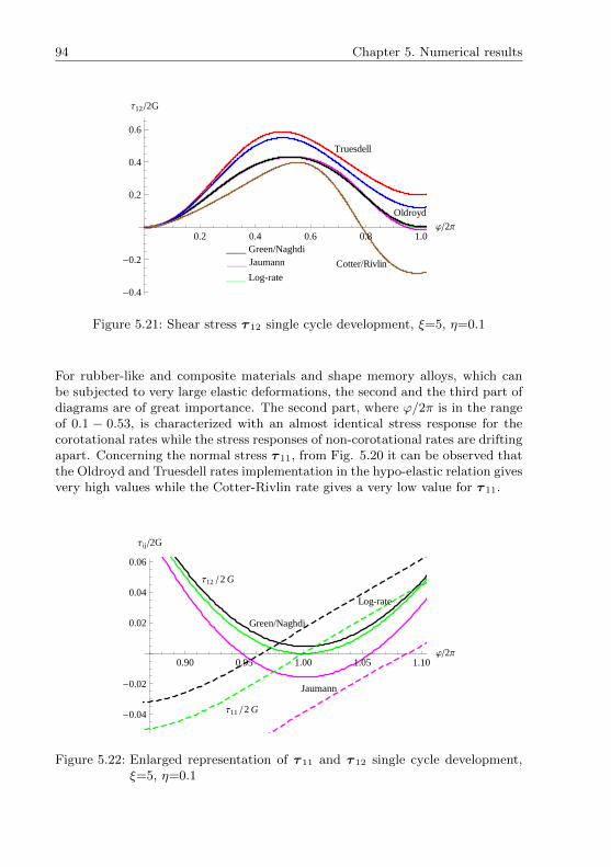
94 Chapter 5. Numerical results
Oldroyd
Truesdell
Cotter/Rivlin
____ Green/Naghdi____ Jaumann
____ Log-rate
0.2 0.4 0.6 0.8 1.0j2Π
-0.4
-0.2
0.2
0.4
0.6
Τ122G
Figure 5.21: Shear stress τ 12 single cycle development, ξ=5, η=0.1
For rubber-like and composite materials and shape memory alloys, which canbe subjected to very large elastic deformations, the second and the third part ofdiagrams are of great importance. The second part, where ϕ/2π is in the rangeof 0.1 − 0.53, is characterized with an almost identical stress response for thecorotational rates while the stress responses of non-corotational rates are driftingapart. Concerning the normal stress τ 11, from Fig. 5.20 it can be observed thatthe Oldroyd and Truesdell rates implementation in the hypo-elastic relation givesvery high values while the Cotter-Rivlin rate gives a very low value for τ 11.
Τ12 2 G
Τ11 2 G
Green/Naghdi
Jaumann
Log-rate
0.90 0.95 1.00 1.05 1.10j2Π
-0.04
-0.02
0.02
0.04
0.06
Τij2G
Figure 5.22: Enlarged representation of τ 11 and τ 12 single cycle development,ξ=5, η=0.1

5.2. Hypo-elasticity 95
The third part of the diagrams is beyond the limit of 0.53 for ϕ/2π where theplots of shear and normal stresses even for the corotational rates are starting todrift apart. At the end of the first cycle some residual normal and shear stressesfor the Green-Naghdi and Jaumann rates occur while the non-corotational ratesproduce extremely high values of residuals. Only the Log-rate gives zero stressvalues at the end of the elastic deformation cycle (see Fig. 5.22). Again, thenormal stresses in 1-1 direction are marked with the dashed lines while the shearstresses are presented by the solid lines.
Τ12 2 G
Τ22 2 G
Τ33 2 G
Τ11 2 G
2 4 6 8 10 12j2Π
-0.4
-0.2
0.2
0.4
Τij2G
Τ12 2 G
Τ22 2 G
Τ33 2 G
Τ11 2 G
20 40 60 80 100j2Π
-0.4
-0.2
0.2
0.4
Τij2G
Figure 5.23: Ten and hundred cycle stress development for the Logarithmic rate,ξ=5, η=0.1
If the continuum square element is subjected to a deformation that repeatscyclically, the stress response error is accumulating for all rates except for theLog-rate. The development of normal and shear stresses during 10 and 100 cycles

96 Chapter 5. Numerical results
for the logarithmic rate has been respectively presented up and down in Figure5.23. It can be seen that the development of all Kirchhoff stress components isregularly periodical with constant magnitudes and without any residuals at theend of each cycle.
Τ12 2 G
Τ22 2 G
Τ33 2 G
Τ11 2 G
2 4 6 8 10j2Π
-0.4
-0.2
0.2
0.4
0.6
Τij2G
Figure 5.24: Ten cycle stress development for the Jaumann rate UMAT, ξ=5,η=0.1
Τ12 2 G
Τ22 2 G
Τ33 2 G
Τ11 2 G
2 4 6 8 10j2Π
-0.4
-0.2
0.2
0.4
0.6
Τij2G
Figure 5.25: Ten cycle stress development for the Jaumann rate ABAQUS, ξ=5,η=0.1
The stress developments obtained using the Jaumann rate in the UMAT sub-routine (see Fig. 5.24) and ABAQUS built-in subroutine for hypo-elastic con-

5.2. Hypo-elasticity 97
stitutive model (see Fig. 5.25) are completely congruent. It is obvious thatthe Jaumann formulation provides an oscillatory stress response for all stresscomponents except τ 33 with variable magnitude of τ 11 and τ 12. The residualstresses at the end of cycles are of non-negligible values and show an oscillatingcharacter as well (see Fig. 5.32).
From Fig. 5.26, where the plots for 100 cycles have been presented, it canbe concluded that the Jaumann rate gives results which are not in accordancewith the physical behaviour of the materials. Therefore, this rate should not beimplemented in the constitutive relations if large cyclic deformation occur.
Τ12 2 G
Τ22 2 G
Τ33 2 G
Τ11 2 G
20 40 60 80 100j2Π
-0.6
-0.4
-0.2
0.2
0.4
0.6
Τij2G
Figure 5.26: Hundred cycle stress development for the Jaumann rate, ξ=5, η=0.1
As in the case of moderate rotations, the stress responses of the Green-Naghdirate formulation show the feature that the magnitude of the shear stress de-creases as the number of cycles increases and after approximately 30 cycles itsvalues are zero which is a totally unrealistic result. After that the maximumshear stress is starting to increase monotonically. The plots for normal stressesτ 11 and τ 22 are drifting away and changing their magnitude with the numberof cycles (see Figures 5.27 and 5.28).
In the case of moderate rotations the Green-Naghdi rate was a more reliablechoice than the Jaumann rate. Here, it can be seen that very high values ofresiduals occur even after a single cycle and their values are monotonically in-creasing as it is recorded in Figure 5.32. All above stated leads us to the con-clusion that for the case of cyclic elastic deformations with large rotations theGreen-Naghdi rate has to be excluded from the hypo-elastic formulations evenfor a low number of repeated cycles.

98 Chapter 5. Numerical results
Τ12 2 G
Τ22 2 G
Τ33 2 G
Τ11 2 G
2 4 6 8 10j2Π
-0.4
-0.2
0.2
0.4
Τij2G
Figure 5.27: Ten cycle stress development for the Green-Naghdi rate, ξ=5, η=0.1
Τ12 2 G
Τ22 2 G
Τ33 2 G
Τ11 2 G
20 40 60 80 100j2Π
-2
-1
1
2
Τij2G
Figure 5.28: Hundred cycle stress development for the Green-Naghdi rate, ξ=5,η=0.1
The Truesdell and the Oldroyd rates give similar stress responses as it is illus-trated in Figures 5.29 and 5.30 where the developments of the shear stress driftapart and increase the magnitude to the unrealistic high values of 30 times forthe Oldroyd rate and 40 times for the Truesdell rate compared with the shearmodulus.

5.2. Hypo-elasticity 99
Τ12 2 G
Τ22 2 G
Τ33 2 G
Τ11 2 G
20 40 60 80 100j2Π
-20
-10
10
20
Τij2G
Figure 5.29: Hundred cycle stress development for the Trusdell rate, ξ=5, η=0.1
Τ12 2 G
Τ22 2 G
Τ33 2 G
Τ11 2 G
20 40 60 80 100j2Π
-10
-5
5
10
15
Τij2G
Figure 5.30: Hundred cycle stress development for the Oldroyd rate, ξ=5, η=0.1
The results for the Cotter-Rivlin rate as well show great deviations from realisticvalues and therefore this rate must be excluded from the constitutive relationconstruction, too.

100 Chapter 5. Numerical results
Τ33 2 GΤ22 2 G
Τ12 2 G
Τ11 2 G
20 40 60 80 100j2Π
-50
-40
-30
-20
-10
10
Τij2G
Figure 5.31: Hundred cycle stress development for the Cotter/Rivlin rate, ξ=5,η=0.1
20 40 60 80 100j2Π
-4
-2
2
4
Τij2G
CotterRivlin
Oldroyd
Truesdell
GreenNaghdi
Jaumann
Τ122G
Τ112G
Figure 5.32: Residual normal and shear stresses for the given rates, ξ=5, η=0.1
In Table 5.4 the normalized residual stresses after 10 cycles have been given for allrates examined. The applied elastic deformation was with very large rotations,i.e. η = 0.2 and ξ = 10. It can be seen that except for the logarithmic rate theresidual stresses are not negligible for the corotational rates and of extremelyhigh values for the non-corotational rates.

5.3. Elastoplasticity 101
Logarithmic Jaumann Green/ Oldroyd Truesdell Cotter/Naghdi Rivlin
τ 11/2G 0.45732e-4 0.035174 2.8971 -43.925 -69.584 -721.76τ 12/2G -0.43250e-4 -0.52436 3.1558 10.437 16.700 -24.353
Table 5.4: Residual stresses after 10 cycles for ξ = 10, η = 0.2
Based on all presented results in this Section it can be concluded that for elasticdeformations with large rotations the only choice among all objective rates wouldbe the logarithmic rate since it is the only rate that gives reliable and physicallyadmissible results for this kind of deformation, i.e. the only elasticity-consistenthypo-elastic constitutive relation would be the one based on the logarithmic rate.
5.3 Elastoplasticity
According to the modern industrial demands the engineers are faced with thetask of finding and constantly improving reliable lifetime assessment proceduresof engineering structures. One of the main problems in fulfilling that goal, forthe structures exposed to elastoplastic deformations, is a proper definition of theconstitutive model that is capable to predict the history dependent behaviour ofthe structural elements. On the other side, for practical applications, the engi-neers sometimes need quick answers which require simple but reliable methods.
Therefore, our intention was to test a simple constitutive model, with only afew necessary parameters, which describes the behaviour of metals during theprocess of small or finite monotonic as well as cyclic elastoplastic deformations.
5.3.1 Small cyclic elastoplastic deformations
In this Section the verification of the numerical model for plastic material be-haviour, proposed in Section 4.5.3, combined with the hypo-elastic model, givenin Section 4.4.2, has been presented.
All necessary material parameters have been estimated from the experimentalresults taken from Westerhoff (1995). The tested material a stainless steel SS304, with elastic constants E = 205.73 GPa and ν = 0.278, has been exposedto uniaxial monotonic and cyclic deformations with various strain ranges, i.e.∆ε = 0.005, 0.015 and 0.02, from which, for our numerical model, the results atroom temperature with a constant strain rate of ε = 10−5s−1 have been selected.The measurement data for monotonic and three cyclic tests have been shown inFigures 5.33 and 5.34, respectively.

102 Chapter 5. Numerical results
Figure 5.33: Monotonic tensile test, source: Westerhoff (1995)
Figure 5.34: Uniaxial cyclic experiments with strain amplitudes ∆ε = 0.005,0.015 and 0.02, source: Westerhoff (1995)
Even though the original INTERATOM model, adopted here as a plasticityconstitutive model, is constructed to anticipate the behaviour of the material atvarious temperature levels, in our model we have confined ourselves to processesat constant room temperature.
5.3. Elastoplasticity 103
Since the test data themselves were no longer available and therefore an op-timization procedure could not be performed, the discussion of the numericalmodel has been done only according to the experimental plots, taken from theaforementioned reference.
First, the stress response due to the uniaxial monotonic tension has been deter-mined using the IA-model for the assumed combined isotropic-kinematic hard-ening as well as for the linear kinematic and linear isotropic hardening indipen-dently. The results are presented in Figure 5.35. It can be observed that theproposed models give stress developments that are in a very good agreementwith the measured values. Thus, it can be concluded that the suggested numer-ical models can be used for the computation of the material behaviour due tomonotonically increasing loading.
Figure 5.35: Numerical results vs monotonic tensile test
The matching between the test and computational results, for the assumed com-bined hardening, can also be seen in the case of alternating loading, given inFigure 5.36.
Concerning the cyclic loading, during the strain-controlled experiment the ex-amined material has shown the hardening behaviour which can be seen in Figure5.34. Applying the same numerical model as tested before, with the hardeningfunctions (4.80), the following results have been obtained for the three differentstrain amplitudes, ∆ε = 0.005, 0.015 and 0.02. The first two cycles for eachstrain range have been given in Figure 5.37.

104 Chapter 5. Numerical results
0.005 0.010 0.015 0.020 0.025h22
-200
-100
0
100
200
300
Σ22 @MPaD
Figure 5.36: Comparison between computation and experiment for the loading-unloading-reloading case
-0.002 -0.001 0.001 0.002h22
-200
-100
100
200
Σ22 @MPaD
-0.006 -0.004 -0.002 0.002 0.004 0.006h22
-300
-200
-100
100
200
300
Σ22 @MPaD
-0.010 -0.005 0.005 0.010h22
-300
-200
-100
100
200
300
Σ22 @MPaD
Figure 5.37: First two cycles of the stress-strain curve for various strain ranges,∆ε = 0.005, 0.015 and 0.02, respectively
Comparing the numerical with the experimental results, it has been detectedthat the stress distributions are qualitatively congruent while quantitatively the

5.3. Elastoplasticity 105
matching between the numerical and experimental plots has not been found. Thereason for that is that the numerical model shows much stronger influence of thehardening than that which can be observed on the test stress-strain responses.As a consequence, numerically the stress saturation is achieved very soon, afterseveral cycles for each strain amplitude. The saturation is noticed in the 15thcycle for ∆ε = 0.005 while for ∆ε = 0.015 and 0.02 it is reached in the 8th and14th cycle, respectively.
The prediction of the cyclic saturated stress amplitudes for each strain range hasbeen very accurate. It can be confirmed with Figure 5.38 where the saturatedexperimental and numerical stress cycles have been presented.
Figure 5.38: Saturated cycles: numerical results (solid line) vs monotonic tensiletest (dashed line), source: Westerhoff (1995)
The computation of the chosen material behaviour using the linearized IA-modelduring the cyclic tests for the three examined strain ranges from the beginningto saturation has been given in Figure 5.39.
As a conclusion it can be said that, concerning the monotonic response, the nu-merical model shows a very good agreement with the experimental results andthus, it can be assumed capable to predict the material behaviour at small aswell as finite strains. On the other side, this numerical calculation shows thenecessity to modify the hardening functions (4.80) in order to obtain a morerealistic model for the cyclic deformations.
Likewise, the numerical model at this stage has shown the lack in describingthe cyclic behaviour at unknown strain ranges, since one of the constituents ofthe proposed model, coefficient gs and c1 consequently, depends on the exper-imentally determined saturated stress. Therefore, in addition, the generalized

106 Chapter 5. Numerical results
evolutionary constitutive model has to be developed in order to predict the be-haviour of the material due to strain ranges that differ from the experimentallyconsidered, especially for the large deformation case.
But the model, in general, has proved itself as a very good initial step in predic-tion of the realistic behaviour of engineering materials.
-0.010 -0.005 0.005 0.010h22
-300
-200
-100
100
200
300
Σ22 @MPaD
Figure 5.39: IA-model uniaxial cyclic response for ∆ε = 0.005, 0.015 and 0.02
All things considered, some tips for future work might be: to find experimentalrecords or carry out experiments in order to obtain data necessary for improvingthe existing linear model. Then, the modification of the hardening functions, orthe coefficients therein, has to be performed in order to calibrate the numericalmodel which prediction would better fit to the experimental data. The evolu-tion equation has to be developed as well to provide that the proposed numericalmodel is usable for unknown strain ranges, too.
Nevertheless, by introducing a nonlinear hardening behaviour of the material,much better results would be achieved and therefore, they would closely coin-cide with the experiments. For example, the proposed numerical model can beimproved if the linear evolution equation (4.79)1 is replaced with the followingnonlinear equation
αLog = c (κ)
(Dp−ακ
). (5.11)
In Figure 5.40, the computational and experimental results during the first cycleof the cyclic deformation for the strain range ∆ε = 0.02 have been compared.The numerical results have been given for the previously suggested IA-modelwith combined isotropic-kinematic hardening and for the improved IA-model

5.3. Elastoplasticity 107
with combined isotropic-nonlinear kinematic hardening. It is obvious that theimproved model give the more realistic stress-strain response.
Some further modifications of the hardening can also be performed and that willbe the topic of future research work.
Figure 5.40: Comparison of IA-model, linear and nonlinear kinematic hardening,with experimental record for strain range ∆ε = 0.02
5.3.2 Finite elastoplastic deformations
The constitutive relations for finite elastoplasticity, derived in Section 4.5.3, havebeen implemented in the ABAQUS/Standard user subroutine UMAT in order tomodel the behaviour of the material exposed to large elastoplastic deformations.The large torsion problem of elastoplastic thin-walled cylindrical tubes with fixedends, reduced to the large simple shear problem of a unit cube, defined in Section5.2.1, has been considered. For the solution of the finite simple shear problem,the objective corotational rates, namely the logarithmic, Jaumann and Green-Naghdi rates, have been used in the constitutive relations and the results havebeen mutually compared.
In order to compare the results for the elastic-perfect plastic and linear kine-matic hardening cases with the corresponding presented in Moss (1984), Szabo& Balla (1989) and Bruhns et al. (2001b and 1999), the same material parame-ters used in the just mentioned references have been adopted for the numericalcalculations.
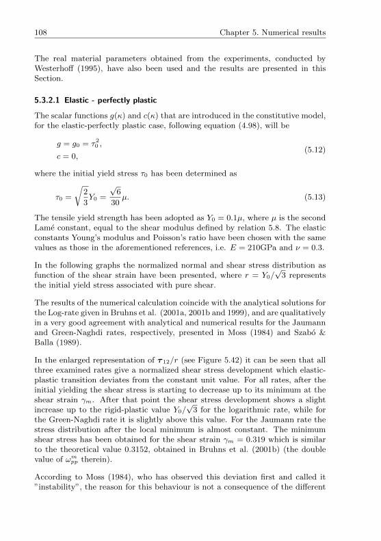
108 Chapter 5. Numerical results
The real material parameters obtained from the experiments, conducted byWesterhoff (1995), have also been used and the results are presented in thisSection.
5.3.2.1 Elastic - perfectly plastic
The scalar functions g(κ) and c(κ) that are introduced in the constitutive model,for the elastic-perfectly plastic case, following equation (4.98), will be
g = g0 = τ20 ,
c = 0,(5.12)
where the initial yield stress τ0 has been determined as
τ0 =
√2
3Y0 =
√6
30µ. (5.13)
The tensile yield strength has been adopted as Y0 = 0.1µ, where µ is the secondLame constant, equal to the shear modulus defined by relation 5.8. The elasticconstants Young’s modulus and Poisson’s ratio have been chosen with the samevalues as those in the aforementioned references, i.e. E = 210GPa and ν = 0.3.
In the following graphs the normalized normal and shear stress distribution asfunction of the shear strain have been presented, where r = Y0/
√3 represents
the initial yield stress associated with pure shear.
The results of the numerical calculation coincide with the analytical solutions forthe Log-rate given in Bruhns et al. (2001a, 2001b and 1999), and are qualitativelyin a very good agreement with analytical and numerical results for the Jaumannand Green-Naghdi rates, respectively, presented in Moss (1984) and Szabo &Balla (1989).
In the enlarged representation of τ 12/r (see Figure 5.42) it can be seen that allthree examined rates give a normalized shear stress development which elastic-plastic transition deviates from the constant unit value. For all rates, after theinitial yielding the shear stress is starting to decrease up to its minimum at theshear strain γm. After that point the shear stress development shows a slightincrease up to the rigid-plastic value Y0/
√3 for the logarithmic rate, while for
the Green-Naghdi rate it is slightly above this value. For the Jaumann rate thestress distribution after the local minimum is almost constant. The minimumshear stress has been obtained for the shear strain γm = 0.319 which is similarto the theoretical value 0.3152, obtained in Bruhns et al. (2001b) (the doublevalue of ωmpp therein).
According to Moss (1984), who has observed this deviation first and called it”instability”, the reason for this behaviour is not a consequence of the different

5.3. Elastoplasticity 109
rates chosen. He suggests that the plastic rotation has to be properly taken intoaccount to achieve the stable solution for an isotropic elastic-perfectly plasticmaterial. For more details see the aforementioned reference.
1 2 3 4 5Γ
0.01
0.02
0.03
0.04
0.05
0.06
Τ11r
GreenNaghdi
Jaumann
Logarithmic
Γm
Figure 5.41: Normalised normal stress vs shear strain for elastic-perfectly plasticbehaviour
1 2 3 4 5Γ
0.9985
0.9990
0.9995
1.0000
Τ12r
Γm
1 2 3 4 5Γ
0.2
0.4
0.6
0.8
1.0
Τ12r
Figure 5.42: Normalized shear stress vs shear strain for elastic-perfectly plasticbehaviour and its enlarged representation

110 Chapter 5. Numerical results
In Bruhns et al. (2001a) the authors have concluded that the instability phe-nomenon occurs due to the absence of hardening. It can be observed from theconsistency condition that in this case the rate of the shear stress and the rate ofthe normal stress have to be of opposite sign. This is the reason why the normalstress distribution shows a monotonic increase while the shear stress decreasesin a so-called boundary layer, i.e. after the yielding where γ = γ0 up to γm, andthe opposite behaviour can be observed after this stationary point. The authorssuggest that hardening has to be taken into accout to obtain a more realisticelastoplastic constitutive model.
GreenNaghdi
Jaumann
Logarithmic
0.5 1.0 1.5 2.0 2.5Γ
0.0006
0.0008
0.0010
0.0012
Τ11r
0.5 1.0 1.5 2.0 2.5Γ
1.01055
1.01060
1.01065
Τ12r
Figure 5.43: Elastic-perfect plasticity: Normalized normal stress developmentand enlarged representation of the normalized shear stress develop-ment for real material parameters

5.3. Elastoplasticity 111
Instead of a very high theoretical value of the initial tensile yield stress usedin the previous example, the more realistic values of Y0 = 159.0MPa, E =205.73GPa and ν = 0.278, taken from Anding (1997) and Westerhoff (1995)for the experimentally tested material, have been used in the second numericalmodel. The boundary layer has not been observed for all examined rates (seeFigure 5.43) but for the logarithmic rate and the Green-Naghdi rate the normalstress distribution monotonically decrease over the whole range of the shearstrain while the shear stress values slowly increase monotonically. Since the timestep used in the numerical integration was 2x10⁻⁵, the shear stress distributionin this case can be assumed as a constant over a whole range of γ.
5.3.2.2 Elastic - linear kinematic hardening
If in the numerical model linear kinematic hardening has been assumed (see Sec-tion 4.5.3.1), the normal and shear stress developments due to large simple shearare strongly dependent on the choice of the hardening parameter c0, introducedin Eq. (4.95)2.
While the Jaumann rate shows oscillatory stress responses for both stresses, forthe logarithmic and Green-Naghdi rates similar monotonically increasing resultshave been obtained for the normal stresses.
GreenNaghdi
Jaumann
Logarithmic
2 4 6 8 10 12Γ
0.2
0.4
0.6
0.8
Τ11Y0
Γkm
Figure 5.44: Normalized normal stress vs shear strain for linear kinematic hard-ening plasticity, c0/r = 0.6
If the hardening is more strong, for example c0/r = 0.6, for the logarithmicrate, after initial yielding the normal stress monotonically increases (see Figure5.44), while the shear stress shows a monotonically growth up to its maximum

112 Chapter 5. Numerical results
value, obtained at shear strain γmk = 2.828 (which corresponds to the doublevalue of ωmkp in Bruhns et al., 2001b) as it has been presented in Fig. 5.45. Afterthat point the shear stress development monotonically decreases approachingthe Y0/
√3 value as γ tends to infinity.
For the Green-Naghdi rate both stress responses show a monotonic growth overthe whole range of γ.
2 4 6 8 10 12Γ0.0
0.5
1.0
1.5
2.0
2.5
3.0
3.5Τ12r
GreenNaghdi
Jaumann
Logarithmic
Γkm
Figure 5.45: Normalized shear stress vs shear strain for linear kinematic harden-ing plasticity, c0/r = 0.6
The afore-presented graphs show that the numerical model gives the stress re-sponses which are in accordance with the analytical solutions given in Bruhnset al. (2001b). In the just cited reference the authors have shown that theelastoplasticity model based on the logarithmic rate gives the prediction of thestress-strain relationship that is in a good agreement with experimental results.
If the hardening is weak, here c0/r = 0.022 has been adopted, after initial yield-ing the shear stress development decreases to a value slightly smaller than theinitial yield stress. After that the shear stress monotonically increases up toits maximum value at γm1 . After having reached its maximum value, the shearstress monotonically falls approaching the value Y0/
√3 for γ tending to infinity,
as it has been shown in the graph given in Figure 5.46.
Concerning the normal stress, contrary to the case of strong hardening wherethe normal stress distribution is monotonically increasing, here two characteris-tic points have been observed (cf. Figure 5.46). After the yield point has beenreached, the normal stress is increasing up to the local maximum at γmk1 from

5.3. Elastoplasticity 113
where the stress drops down to its local minimum at γmk2. After this turning pointthe τ11 again increases monotonicaly. The Jaumann rate in both Figures ex-hibits an unrealistic oscillating behaviour, whereas the Green-Naghdi rate leadsto much too high shear stresses.
GreenNaghdi
Jaumann
Logarithmic
0 2 4 6 8 10 12Γ0.97
0.98
0.99
1.00
1.01
1.02Τ12r
Γ1m
Figure 5.46: Normalized shear stress vs shear strain for linear kinematic harden-ing plasticity, c0/r = 0.022
0 2 4 6 8 10 12Γ0.00
0.01
0.02
0.03
0.04
0.05Τ11Y0
GreenNaghdi
Jaumann
Logarithmic
Γk1m Γk2
m
Figure 5.47: Normalized normal stress vs shear strain for linear kinematic hard-ening plasticity, c0/r = 0.022

114 Chapter 5. Numerical results
In a second example the material parameters obtained from the experimentsby Westerhoff (1995) have been used and the kinematic hardening modulus c0,according to Eq. (4.96), has been attained as
c0 =2
3B = 1945.008MPa. (5.14)
The numerical calculations gave the following results if the logarithmic rate wasused.
1 2 3 4 5Γ
5
10
15
Τ11Y0
0 1 2 3 4 5Γ0
5
10
15
Τ12r
Figure 5.48: Normalized normal and shear stress vs shear strain for the materialparameters according to Westerhoff (1995)
It can be seen that the kinematic hardening is very strong, as it was alreadyconcluded in Section 5.3.1. From the numerical calculations the maximum shearstress has been achieved as τm12real = 1381.88MPa for γm = 3.03 which is inaccordance with the analytical value τm12real = 1380.748MPa , obatined usingEq. (6.19) from Bruhns et al. (2001b), for γm = 3.0176 (the double value of ωmkpfrom the just mentioned reference).
Assuming the same material parameters as in the previous example, the platewith a hole that undergoes large axial elastoplastic deformation has been tested.The assumed model has been taken as previously introduced (see Figure 5.5).Here, the prescribed displacement in the axial direction has been 2.5mm.
Due to the symmetry of the plate and loading, only a quarter of the plate hasbeen considered in the numerical calculations. The deformed and undeformedconfigurations as well as the normal stress distribution in the plate at the endof deformation have been given in Figure 5.49.

5.3. Elastoplasticity 115
Figure 5.49: Plate with a hole in tension: Undeformed and deformed configura-tion and normal stress distribution for large elastoplastic deforma-tion with linear kinematic hardening
With the Log-rate implemented in the constitutive relations, the developmentof the normalized normal stress for the node at the hole that undergoes themaximum stress has been presented in the following figure.
0.00 0.01 0.02 0.03 0.04 0.05h220.0000
0.0005
0.0010
0.0015
0.0020
0.0025Σ222G
Figure 5.50: Plate with a hole in tension: Normalized normal stress distributionfor large elastoplastic deformation with linear kinematic hardening

6 Concluding remarks
6.1 Summary and conclusions
The numerical implementation of the self-consistent Eulerian finite elastoplastic-ity theory, based on the logarithmic rate and the additive decomposition of thenatural deformation rate (stretching), in the commercial finite element softwareand its validation have been the main tasks of this treatise.
Alongside the Log-rate, the Jaumann and Green-Naghdi rates, as corotational,and the Truesdell rate, the Oldroyd rate and the Coter-Rivlin rate, as non-corotational rates, have been implemented in the constitutive models as well.The proposed numerical frameworks were verified on several benchmark exam-ples and the results were compared mutually and with the relevant literature.In order to preserve objectivity of the Eulerian rate model special attention isgiven to the incremental objectivity.
The stress-strain prediction due to large elastic deformations, usually met in abroad class of rubber-like materials, shape memory alloys, etc., has been modeledby the hypo-elastic constitutive relation, i.e. by the linear relationship betweenthe objective rate (increment) of the Kirchhoff stress and the rate (increment)of its work-conjugate pair, the Eulerian Hancky strain, via a constant isotropic4th-order tensor. The rate form of the hypo-elastic constitutive relation qualifiesit to become a basic constituent in the structure of the adopted Eulerian ratetheory of finite elastoplasticity, too, while the plasticity part has been modeledby the associated flow rule.
Concerning the pure elastic deformation, the numerical calculations have provedthat, opposite to the other tested rates, the logarithmic rate predicts the stablesolutions with no residuals in the closed elastic strain path, and thus confirmingthat the hypo-elastic constitutive relation based on the Log-rate is self-consistentin the sense of elasticity.
The thesis has shown that the occurrence of the finite rotations in total defor-mation significantly influences stress responses. In the case of small rotationsall examined objective corotational rates give the accurate results while the re-liability of the Jaumann and Green-Naghdi rates is decreasing with the increaseof rotations. For cyclic deformations with moderate and large rotations, thepreviously mentioned rates produce high values of residual stresses at the endof the cycle, especially if the deformation is repeated in large number of cycles,
116

6.2. Possible extensions of the present research 117
which is the usual case. The Log-rate has proved itself as the only one thatgives responses in accordance with those theoretically expected. In this thesisit has been shown that the non-corotational rates have to be excluded from theconstitutive relations even for moderately large rotations.
The numerical implementation is thereafter extended to elastoplastic deforma-tions. Constitutive relations for finite plasticity, based on the INTERATOMmodel which originally has been established for the small deformation case, havebeen derived and numerically implemented. The behaviour of the material dur-ing small monotonic and cyclic elastoplastic deformations and finite monotonicelastoplastic deformations has been tested, too. The simple constitutive modelconcerning combined isotropic-kinematic hardening, established by introducinga few material constants, has been proposed and its stress-strain prediction hasbeen compared to the experimental results. It has been concluded that the pro-posed model gives the results that are in a very good agreement with monotonictests and in a qualitatively agreement with experiments for cyclic behaviour andtherefore can be used as an initial step in the prediction of a realistic behaviourof engineering materials. Some improvements of the existing model have beenproposed as well.
6.2 Possible extensions of the present research
The proposed Eulerian finite elastoplasticity model can be extended in severalways.
Although the current formulation of the given constitutive model focuses on rate-independent elastoplasticity, an extension to visco-plasticity is possible. More-over, the underlying IA model has been constructed to describe a visco-plasticbehaviour (at higher temperatures). Here, isothermal processes have been thesubject of research, but it can be broadened to adopt thermal effects as well.
The proposed constitutive model of elastoplasticity relies on experimental re-sults. In order to provide that the existing numerical model can be used forthe strain ranges that have not been tested, the proper evolution constitutiveequation has to be developed.
The first improvement that can be made, and that was already indicated andbegun in this work, is the introduction of the nonlinear hardening behaviour ofmaterials.
Any step forward towards a generalization of the model would demand morematerial parameters and would make the analysis more complex. Some of thebasic hypotheses than must be reconsidered.
In order to ensure more practical application of the proposed models, more com-

118 Chapter 6. Concluding remarks
plex engineering structures with more realistic loadings have to be treated aswell. One of these applications can be a modeling of metal forming processeswhere the spring effect should be properly taken into account.
But as a first step to improve the model, the implementation of the log rate intoa commercial finite element code and its validation have been done with thisthesis.

Bibliography
ABAQUS (2013): Documentation, Dassault Systemes Simulia Corp., Provi-dence, RI, USA.
Anand, L. (1979): On H. Hencky’s approximate strain-energy function for mod-erate deformations, in: J. Appl. Mech., Volume 46, 78–82.
Anand, L. (1986): Moderate deformations in extension-torsion of incompressibleisotropic elastic materials, in: J. Mech. Phys. Solids, Volume 34, 293–304.
Anding, D. K. (1997): Zum simultanen Bestimmung matmaterialabhangigerKoeffizienten inelastischer Stoffgesetze 1997, Ph. D. thesis, Mitteilungen ausdem Institut fur Mechanik 109, Ruhr-Universitat Bochum.
Atluri, S. N. (1984): On constitutive relations at finite strain: hypoelasticityand elastoplasticity with isotropic or kinematic hardening , in: Computer Meth.Appl. Mech. Engng., Volume 43, 137–171.
Basar, Y. & Weichert, D. (2000): Nonlinear Continuum Mechanics of Solids,Springer 2000.
Bazant, Z., Gattu, M. & Vorel, J. (2012): Work conjugacy error in com-mercial finite-element codes: its magnitude and how to compensate for it , in:Proc. Roy. Soc. A, Volume 468, 3047–3058.
Bazant, Z. & Vorel, J. (2014): Energy-Conservation Error Due to Use ofGreen-Naghdi Objective Stress Rate in Commercial Finite-Element Codes andIts Compensation, in: ASME J. Appl. Mech., Volume 81(2).
Belytschko, T., Liu, W. K. & Moran, B. (2000): Nonlinear finite elementsfor continua and structures, John Wiley & Sons, Ltd. 2000.
Bertram, A. (2012): Elasticity and Plasticity of Large Deformations, thirdedition Edition, Springer-Verlag Berlin Heidelberg 2012.
Besson, J., Cailletaud, G., Chaboche, J.-L., Forest, S. & Bletry, M.(2009): Non-Linear Mechanics of Materials, Springer 2009.
Bonet, J. & Wood, R. (2008): Nonlinear Continuum Mechanics for FiniteElement Analysis, 2nd Edition, Cambridge University Press 2008.
Bruhns, O. T. (2003): Advanced Mechanics of Solids, Springer, Berlin 2003.
119

120 Bibliography
Bruhns, O. T. (2005): A continuum theory of plasticity , lecture notes,SEEFORM PhD studies, Skopje, 2005.
Bruhns, O. T. (2014): The Prandtl-Reuss equations revisited , in: ZAMM · Z.Angew. Math. Me., Volume 94, 3, 187–202.
Bruhns, O. T. & Anding, D. (1999): On the simultaneous estimation of modelparameters used in constitutive laws for inelastic material behaviour , in: Int.J. Plasticity, Volume 15, 1311–1340.
Bruhns, O. T., Boecke, B. & Link, F. (1984): The constitutive relations ofelastic-inelastic materials at small strains, in: Nucl. Eng. Des., Volume 83,325–331.
Bruhns, O. T., Chaboche, J. L., Eikhofft, J. V. D. & White, P. S. (1988):Constitutive modelling in the range of inelastic deformation, Technical report,Commission of the European Communities, 1988.
Bruhns, O. T., Meyers, A. & Xiao, H. (2001a): Analytical perturbationsolution for large simple shear problems in elastic-perfect plasticity with thelogarithmic stress rate, in: Acta Mechanica, Volume 151, 31–45.
Bruhns, O. T., Meyers, A. & Xiao, H. (2004): On non-corotational rates ofOldroyd’s type and relevant issues in rate constitutive formulations, in: Proc.Roy. Soc. A, Volume 460, 909–928.
Bruhns, O. T., Xiao, H. & Meyers, A. (1999): Self-consistent Eulerian ratetype elastoplasticity models based upon the logarithmic stress rate, in: Int. J.Plasticity, Volume 15, 479–520.
Bruhns, O. T., Xiao, H. & Meyers, A. (2001b): Large simple shear andtorsion problems in kinematic hardening elastoplasticity with logarithmic rate,in: Int. J. Solids Struct., Volume 38, 8701–8722.
Chaboche, J. L. (2008): A review of some plasticity and viscoplasticity consti-tutive theories, in: Int. J. Plasticity, Volume 24, 1642–1693.
Cotter, B. A. & Rivlin, R. S. (1955): Tensors asosiated with time-dependentstress, in: Q. Appl. Math., Volume 13, 177–182.
Dienes, J. K. (1979): On the analysis of rotation and stress rate in deformingbodies, in: Acta Mechanica, Volume 32, 217–232.
Doyle, T. C. & Ericksen, J. L. (1956): Nonlinear elasticity , in: Adv. Appl.Mech., Volume 4, 53–115.
Dunne, F. & Petrinic, N. (2005): Introduction to Computational Plasticity ,Oxford University Press 2005.

Bibliography 121
Green, A. E. & McInnis, B. C. (1967): Generalized hypoelasticity , in: P. Roy.Soc. A, Volume 57, 220–230.
Green, A. E. & Naghdi, P. M. (1965): A general theory of an elasto-plasticcontinuum, in: Arch. Ration. Mech. An., Volume 18, 251–281.
Haupt, P. (2000): Continuum Mechanics and Theory of Materials, Springer-Verlag, Berlin Heidelberg 2000.
Hencky, H. (1928): Uber die Form des Elastizitatsgesetzes bei ideal elastischenStoffen, in: Z. Techn. Phys., Volume 9, 215–223.
Hencky, H. (1929a): Das Superpositionsgesetz eines endlich deformierten re-laxationsfahigen elastischen Kontinuums und seine Bedeutung fur eine exakteAbleitung der Gleichungen fur die zahe Flussigkeit in der Eulerschen Form,in: Ann. Phys., Volume 5, 617–630.
Hencky, H. (1929b): Welche Umstande bedingen die Verfestigung bei der bild-samen Verformung von festen isotropen Korpern? , in: Z. Phys., Volume 55,145–155.
Hill, R. (1950): The Mathematical Theory of Plasticity , Clarendon Press, Ox-ford 1950.
Hill, R. (1968): On constitutive inequalities for simple materials, in: J. Mech.Phys. Solids, Volume 16, 229–242; 315–322.
Hill, R. (1970): Constitutive inequalities for isotropic elastic solids under finitestrain, in: Proc. Roy. Soc. London A, Volume 326, 131–147.
Hill, R. (1978): Aspects of invariance in solid mechanics, in: Avdv. Appl.Mech., Volume 18, 1–75.
Jaumann, G. (1911): Geschlossenes System physikalischer und chemischer Dif-ferentialgesetze, in: Akad. Wiss. Wien Sitzber. (IIa), Volume 120, 385–530.
Johnson, G. C. & Bammann, D. J. (1984): A discussion of stress rates infinite deformation problems, in: Int. J. Solids Struct., Volume 20, 725–737.
Kang, G., Bruhns, O. & Sai, K. (2011): Cyclic polycrystalline visco-plasticmodel for ratchetting of 316L stainless steel , in: Comput. Mater. Sci., Vol-ume 50, 1399–1405.
Khan, A. S. & Huang, S. (1995): Continuum theory of plasticity , John Wiley& Sons, Inc. 1995.

122 Bibliography
Kojic, M. & Bathe, K. J. (1987): Studies of finite element procedures stresssolution of a closed elastic strain path with stretching and shearing using theupdated Lagrangian-Jaumann formulation, in: Computer Struct., Volume 26,175–179.
Lehmann, T. (1972): Anisotrope plastische Formanderungen, in: Romanian J.Techn. Sci. Appl. Mechanics, Volume 17, 1077–1086.
Lehmann, T. (1982): Some remarks on the decomposition of deformations andmechanical work , in: Int. J. Engng Sci., Volume 20, 2, 281–288.
Lehmann, T. (1989): Some Thermodynamical Considerations on Inelastic De-formations Including Damage Processes, in: Acta Mech., Volume 79, 1–24.
Lehmann, T., Guo, Z. H. & Liang, H. Y. (1991): The conjugacy betweenCauchy stress and logarithm of the left stretch tensor , in: Eur. J. Mech.A/Solids, Volume 10, 395–404.
Lemaitre, J. & Chaboche, J.-L. (1990): Mechanics of solid materials, Cam-bridge University Press 1990.
Lin, R., Schomburg, U. & Kletschkowski, T. (2003): Analytical stress sso-lution of a closed deformation path with stretching and shearing using thehypoelastic formulations, in: Eur. J. Mech. A/Solids, Volume 22, 443–461.
Lubarda, V. A. (2001): Elastoplasticity Theory , CRC Press, New York 2001.
Lubliner, J. (2008): Plasticity Theory , Dover Publications, Inc. Mineola, NewYork 2008.
Luig, P. (2008): A consistent Eulerian rate model for shape memory alloys2008, Ph. D. thesis, Mitteilungen aus dem Institut fur Mechanik 148, Ruhr-Universitat Bochum.
Malvern, L. E. (1969): Introduction to the mechanics of a continuous medium,Prentice-Hall, Inc., Englewood Cliffs, New Jersey 1969.
Marsden, J. E. & Hughes, T. J. R. (1983): Mathematical foundations ofelasticity , Dover Publications, Inc., Mineola, New York 1983.
Mase, G. F. & Mase, G. T. (1999): Continuum Mechanics for Engineers, 2nded., CRC Press, Boca Raton, FL 1999.
Meyers, A., Xiao, H. & Bruhns, O. T. (2003): Elastic Stress Ratchetting andCorotational Stress Rates, in: Technische Mechanik, Volume 23, 2-4, 92–102.
Meyers, A., Xiao, H. & Bruhns, O. T. (2006): Choice of objective rate in sin-gle parameter hypoelastic deformation cycles, in: Computers and Structures,Volume 84, 1134–1140.
Bibliography 123
Micunovic, M. (1990): Applied continuum mechanics (in Serbian), Naucnaknjiga, Beograd 1990.
Moss, C. (1984): On instabilities in large deformation simple shear loading , in:Computer Meth. Appl. Mech. Engng., Volume 46, 329–338.
Naghdi, P. M. (1990): A critical review of the state of finite elasoplasticity , in:Z. Angew. Math. Phys., Volume 41, 315–394.
Nagtegaal, J. C. & de Jong, J. E. (1982): Some aspects of non-isotropicworkhardening in finite strain plasticity , in: H., L. E. & Mallett, R. L.(Eds.): Plasticity of Metals at Finite Strain: Theory, Computation and Ex-periment , Stanford University 1982, pp. 65–106.
Ogden, R. W. (1984): Non-linear elastic deformations, Dover Publications,Inc. Mineola, New York 1984.
Oldroyd, J. G. (1950): On the formulation of rheological equations of state,in: Proc. Roy. Soc. London A, Volume 200, 523–541.
Pohe, J. & Bruhns, O. T. (1993): On a thermodynamical consistent constitu-tive law based on the concept of internal variables, in: Mech Res Commun.,Volume 20, 2, 99–105.
Reinhardt, W. D. & Dubey, R. N. (1996): Coordinate-independent represen-tation of spin tensors in continuum mechanics, in: J. Elasticity, Volume 42,133–144.
Seth, B. R. (1964): Generalized strain measure with applications to physicalproblems, in: Reiner, M. & Abir, D. (Eds.): Second-order effects in elastic-ity, plasticity and fluid dynamics, Pergamon Press 1964, pp. 162–172.
Simo, J. C. (1988): A framework for finite strain elastoplasticity based on max-imum plastic dissipation and the multiplicative decomposition: Part I. Con-tinuum formulation, in: Comput. Meths. Appl. Mech. Engrg., Volume 66,199–219.
Simo, J. C. & Hughes, T. J. R. (1998): Computational inelasticity , SpringerVerlag 1998.
Simo, J. C. & Pister, K. S. (1984): Remarks on rate constitutive equations forfinite deformation problems: computational implications, in: Comput. Meths.Appl. Mech. Engrg., Volume 46, 201–215.
Szabo, L. & Balla, M. (1989): Comparison of stress rates, in: Int. J. SolidsStructures, Volume 25, 279–297.
124 Bibliography
Truesdell, C. (1953): Corrections and additions to ’The mechanical founda-tions of elasticity and fluid dynamics’ , in: J. Ration. Mech. Anal., Volume 2,593–616.
Truesdell, C. (1955a): Hypo-elasticity , in: J. Rat. Mech. Anal., Volume 4,83–133.
Truesdell, C. (1955b): The simple rate theory of pure elasticity , in: Comm.Pur. Apl. Math., Volume 8, 123–132.
Truesdell, C. (1956): Hypo-elastic shear , in: J. Appl. Phys., Volume 27, 441–447.
Truesdell, C. & Noll, W. (2004): The non-linear field theories of mechanics,3rd edition Edition, Springer Verlag 2004.
Truesdell, C., Noll, W. & Antman, S. (2004): The Non-Linear Field The-ories of Mechanics, Volume 3 of The non-linear field theories of mechanics,Springer 2004.
Sumarac, D. & Perovic, Z. (2015): Cyclic plasticity of trusses, in: Arch.Appl. Mech., Volume 85, 9, 1513–1526.
Westerhoff, B. (1995): Eine Untersuchung zum geschwindigkeitsabhangigenVerhalten von Stahl 1995, Ph. D. thesis, Mitteilungen aus dem Institut furMechanik 99, Ruhr-Universitat Bochum.
Xiao, H., Bruhns, O. & Meyers, A. (1988): Objective corotational rates andunified work-conjugacy relation between Eulerian and Lagrangean strain andstress measures, in: Arch. Mech., Volume 50, 6, 1015–1045.
Xiao, H., Bruhns, O. T. & Meyers, A. (1997a): Hypo-elasticity model basedupon the logarithmic stress rate, in: J. Elasticity, Volume 47, 51–68.
Xiao, H., Bruhns, O. T. & Meyers, A. (1997b): Logarithmic strain, logarith-mic spin and logarithmic rate, in: Acta Mech., Volume 124, 89–105.
Xiao, H., Bruhns, O. T. & Meyers, A. (1998a): On objective corotationalrates and their defining spin tensors, in: Int. J. Solids Structures, Volume 35,30, 4001–4014.
Xiao, H., Bruhns, O. T. & Meyers, A. (1998b): Strain rates and materialspins, in: J. Elasticity, Volume 52, 1–41.
Xiao, H., Bruhns, O. T. & Meyers, A. (1998c): Objective corotational ratesand unified work-conjugacy relation between Eulerian and Lagrangean strainand stress measures, in: Arch. Mech., Volume 50, 1015–1045.

Bibliography 125
Xiao, H., Bruhns, O. T. & Meyers, A. (1999): Existence and uniqueness
of the integrable-exactly hypoelastic equationτ ∗ = λ(trD)I + 2µD and it’s
significance to finite inelasticity , in: Acta Mech., Volume 138, 31–50.
Xiao, H., Bruhns, O. T. & Meyers, A. (2000a): The choice of objective ratesin finite elastoplasticity: general results on the uniqueness of the logarithmicrate, in: P. Roy. Soc. A, Volume 456, 1865–1882.
Xiao, H., Bruhns, O. T. & Meyers, A. (2000b): A consistent finite elasto-plasticity theory combining additive and multiplicative decomposition of thestretching and the deformation gradient , in: Int. J. Plasticity, Volume 16,143–177.
Xiao, H., Bruhns, O. T. & Meyers, A. (2005): Objective stress rates, path-dependence properties and non-integrability problems, in: Acta Mech., Vol-ume 176, 135–151.
Xiao, H., Bruhns, O. T. & Meyers, A. (2006a): Elastoplasticity beyond smalldeformations, in: Acta Mech., Volume 182, 31–111.
Xiao, H., Bruhns, O. T. & Meyers, A. (2006b): Objective stress rates, cyclicdeformation paths, and residual stress accumulation, in: ZAMM · Z. Angew.Math. Me., Volume 86, 11, 843–855.
Xiao, H., Bruhns, O. T. & Meyers, A. (2007): Thermodynamic laws andconsistent Eulerian formulation of finite elastoplasticity with thermal effects,in: J. Mech. Phys. Solids, Volume 55, 338–365.
Zaremba, S. (1903): Sur une forme perfectionee de la theorie de la relaxation,in: Bull. Intern. Acad. Sci. Cracovie, , 594–614.