EME-451 CAPSTONE I

_________________________________________________________________________________________________________

Numerical and Experimental Investigation of multiphase flows.

Fundamental and Applied studies

_________________________________________________________________________________________________________

Student name and ID: Asset Zhamiyev

Nurzhan Maldenov

Bekbolat Adekenov

Arman Abylkassimov

Supervisor: Sholpan Sumbekova

Michael Yong Zhao

Date of Submission: 24.11.2019

Abstract

Multiphase flows can be met both in nature and in industrial processes. The particular case of

multiphase flows is particle-laden flows, consisting of fluid phase and particle phase. Study is

aimed at the investigation of the dynamics of particles in laminar and turbulent flows. The

dynamics of particles depends on their physical properties. The study of the particle’s dynamics in

turbulent flow consisted of three parts: simulation of homogeneous isotropic turbulence (HIT),

simulation of particle-laden flows and investigation of particles’ pair dispersion. Initially, the

turbulent flow was simulated in OpenFOAM via Large Eddy simulation (LES) and Direct Navier

Stokes (DNS) methods. Then not decaying homogeneous isotropic turbulence was achieved by

addition of forcing term. The effect of different values of forcing constant on turbulent flow was

investigated. The mesh convergence study was performed for LES and DNS. Results showed

convergence in LES simulations and the reduction of volume-averaged velocity fluctuations (U’)

in DNS with an increase of the number of mesh elements. The particle phase simulation was

performed in Matlab and CFDEM. The simulation in Matlab revealed several constraints. The

simulation of particles with turbulence phase for a short period of time was performed in CFDEM.

However, due to the decaying nature of the flow, the investigation of particles’ trajectories could

not be performed. The pair dispersion of inertial particles in turbulent flow was investigated for

available experimental data. The results were represented on graphs with normalized scales. The

correlation between the velocity of flow and the normalized value of the initial separation was

determined. The mean square separation does not change significantly until the first decade. The

motion of clots in blood flow was numerically simulated using Ansys Fluent package. The mesh

convergence study was performed and the velocity of the particles in blood flow was analyzed.

The results obtained for blood flow showed distribution close to Gaussian. The preliminary

experiment was conducted for small particles of smoke. The smoke cloud was detected via the

image intensity analysis.

Table of Contents

1. Introduction ................................................................................................................................. 4

2. Background information ............................................................................................................. 6

2.1 Homogeneous Isotropic Turbulence ..................................................................................... 6

2.2 Dynamics of particle phase ................................................................................................... 7

2.3 Murray’s Law ........................................................................................................................ 9

3. Literature review ....................................................................................................................... 10

4. Methodology ............................................................................................................................. 13

4.1 Flow simulations ................................................................................................................. 13

4.2 Simulation of particle phase ................................................................................................ 15

4.3 Particles’ pair dispersion ..................................................................................................... 16

4.4.1 Simulations of particles (blood clots) in arteries .............................................................. 18

4.4.2 Mesh convergence study .................................................................................................. 18

4.5 Experimental part ................................................................................................................ 20

5. Results and discussion .............................................................................................................. 22

5.1 Simulation of flow ............................................................................................................... 22

5.2 Simulation of particle phase ................................................................................................ 27

5.3 Pair dispersion of inertial particles in turbulent flow .......................................................... 30

5.4 Multiphase in coronary arteries ........................................................................................... 32

5.5 Experimental results ............................................................................................................ 43

6. Conclusion ................................................................................................................................ 44

7. Reference list ............................................................................................................................ 46

Appendix ....................................................................................................................................... 49

1. Introduction Multiphase flows are widespread and can be found both in natural phenomena such as the

formation of clouds and sedimentation in rivers [1] and numerous industrial processes including

coal combustion, pipeline pneumatic transport [2, 3]. Therefore, the study of the nature of these

processes is important both for fundamental science and for industry. The particular case of

multiphase flows is particle-laden flows. Particle-laden flows consist of fluid and particles phases,

typically liquid droplets or solid particles. The particle-laden flows can be laminar and turbulent.

The dynamics of particles in a turbulent flow is affected by the flow; however, the degree of

influence of the flow on the motion of particles depends on the physical properties of the particles.

The main mechanisms influencing the behavior of particles in the flow are viscous drag exerted

from turbulence to particles and gravitational force. If the density of particles is approximately the

same as of fluid (neutrally buoyant particles) and the size of particles is small (much less than the

smallest turbulent eddies at the Kolmogorov scale), particles behave as tracers following the

motion of the flow [4]. Kolmogorov scale is the smallest scale of turbulence, which is characterized

by domination of viscous forces over fluid inertia [5]. The acceleration and vorticity of the

turbulence in Kolmogorov scale is maximum. Being less than Kolmogorov scale tracers are

exposed mostly to the drag force [6]. However, if the density of particles is considerably smaller

or larger than the density of fluid, or when the size of particles becomes of the same order as the

turbulent eddies, the motion of particles is affected by the inertial effects and gravitational force.

Such particles are called inertial particles and their motion deviates from the flow. The inertial

effects of particles is quantified by calculation of Stokes number (St).

𝑆𝑡 =𝜏𝑝

𝜏𝜂, (1)

Where 𝜏𝑝 – particle response time, 𝜏𝜂 – Kolmogorov time scale

Inertial particles lag behind the flow, and particle response time is time required to particle to

respond to the change of the flow’s velocity. Kolmogorov time scale – time of energy dissipation

at Kolmogorov scale [5]. Being in a turbulent flow, inertial particles are centrifuged due to the

interaction with turbulent vortices and cluster in the zones of high strain and low vorticity [6].

Finally, as the time passes the particle settle under the influence of gravitation. The study

conducted by Wang and Maxey [7] demonstrated that the preferential sweeping is the prevailing

mechanism in a turbulent flow. The inertial particles distribute unevenly in a turbulent non-

uniform flow, clustering in the regions of high strain rate and low vorticity. The mechanism of

accumulation of particles in certain regions is called the preferential concentration [8]. Maxey

demonstrated that the preferential concentration results in a bias of particles’ motion and enhanced

settling velocity.

The reduction of particle settling velocity is related to three mechanisms: nonlinear drag,

vortex trapping and loitering effect [9]. The different studies conducting on the effect of nonlinear

drag on the reduction of particles’ settling rate provide controversial data. The results obtained by

Mei [10] and Stout et al. [11] demonstrated the reduction of settling velocity related to nonlinear

drag. The results obtained by Stout et al. show that the reduction of average settling velocity may

exceed 35%. At the same time, the analytical solution derived by Nielsen [12] indicated the

negligible effect of drag (>10-5VT). Vortices in a turbulent flow tend to trap inertial particles

temporally (forming vortex trap) and transport them over certain distances, finally flinging

particles [13]. Being trapped in vortices particles are affected by the motion of vortices and,

therefore, their settling rate is reduced. The numerical results of Vilela and Motter [14]

demonstrated the possibility of the vortex traps in the presence of large gravitational force for

aerosol particles in leepfrog system and blinking vortex system. The loitering effect was firstly

observed by Nielsen [12]. Loitering is the effect describing the reduction of particle settling rate

happening when fast-moving particles pass through regions of flow moving upward and

downward. The particle requires more time to cross the upward-moving regions. The observations

of Nielsen were further confirmed by Good et al. [15].

The particles-laden laminar flows characterized by low velocity as well as high viscosity could

be found in engineering applications involving flows in circular ducts, natural convection and air

ventilating processes. The-two phase flows in coronary arteries, in which the carrier fluid is non-

Newtonian blood and the particle phase represented by fragmented blood clots proceed under

laminar regime. That is due to the high blood viscosity and relatively low values of inner artery

diameters and average outlet velocities. The curved circular blood vessels that supply oxygen-rich

blood to the myocardium are defined as coronary arteries. The Reynolds number based on inlet

and outlet velocities are found to be less than 2300 implying laminar flow field [16]. The stable

and continuous blood supply ought to be delivered to the heart to sustain its optimal cardiac

functions and cycle. Atherosclerosis, which is the form of cardiovascular disease, contributes to

the formation of plaque on the vessel wall. As a results, the coronary artery narrows, thereby

restricting the blood supply to myocardium. Stenosis is related to the increased plaque

accumulation and results to the narrowing of aortic valve area, leading to the rapid advancement

of the coronary artery disease [17]. The alteration of blood flow due to narrowing artery facilitate

clots formation. The fragmented clots lag behind the blood flow due to higher density and behave

as inertial particles with complex flow structures dispersed in blood stream [18]. The clot

formation leads to an advancement of unwanted diseases like stroke, paralysis, heart attack that

require immediate medical treatment. According to World Health Organization data (2019), the

cardiovascular disease (CVD) is the major cause of people mortality all over the globe. Around

80% of all deaths worldwide associated with CVDs occur in countries with low and middle income

[19]. The investigation of dynamics of inertial particles in laminar flow may be used for

determination of the location of stenosis in arteries. Thereby, the amount of deaths due to CVDs

can be reduced.

This paper is aimed at in-depth investigation of the multiphase flows on the examples of

laminar and turbulent particle-laden flows. The study consists of the numerical simulations of

inertial particles in turbulent flow and applied biomechanics study – the investigation of the

particles in arteries. Additionally, the study contains experimental part. The simulations of the

particle-laden turbulent flow are performed via direct Navier-Stokes (DNS) and large eddy

simulations (LES) methods in OpenFOAM software. The simulations of particle phase are

performed in Matlab and CFDEM. The simulation of the multiphase flow in arteries are performed

in ANSYS Fluent package.

2. Background information

2.1 Homogeneous Isotropic Turbulence

Homogeneous isotropic turbulence (HIT) is one of the forms of idealistic turbulence flow

that can be modeled with numerical simulation. Statistical parameters are invariant of coordinate

system of domain of study in HIT. DNS and LES are commonly applied to HIT flows and

generated turbulence field is used in particle tracking simulations [19][20][21]. HIT is not

statistically stationary and velocity fluctuations tend to decrease to zero with time evolution until

it reaches zero. Statistically stationary field is achieved when the field averaged dissipation rate is

equal to energy addition rate. [21] Stochastic forcing mechanism is developed based on the

assumption that small scales are not affected by the mechanisms of forcing scheme if there is the

same level of energy-production and dissipation in a turbulent flow. Based on this method, velocity

field is transformed into Fourier space as shown in equation below,

�̃�(𝑘, 𝑡) = ∑ ∑ ∑ 𝑢(𝑥, 𝑡)𝑒−𝑖𝑘∙𝑥𝑁𝑁𝑁 , (2)

Where 𝑢(𝑥, 𝑡) – velocity at grid point inflow domain, �̃�(𝑥, 𝑡) – corresponding Fourier coefficient

to this point. Forcing is added to acceleration equation as shown in (3) 𝜕𝑢(𝑥,𝑡)

𝜕𝑡= �̃�(𝑘, 𝑡) + �̃�𝐹(𝑘, 𝑡) (3)

Where �̃�𝐹(𝑘, 𝑡) is forcing term that is non-zero for𝑘 ∈ [0, 𝐾𝐹]. Forcing acceleration term is

modelled with Uhlenbeck-Ornstein (UO) random process [22] where main controllable variables

are acceleration variance 𝜎 and forcing time constant (𝛼).

𝛼 =1

𝑡𝑓 (4)

Where tf – time period in which the forcing term is added to the flow (forcing time)

The relation between the forcing time scale and HIT flow field properties were studied when

stochastic forcing was implied to add kinetic energy at large scales. Results of DNS revealed that

flow dissipation rate and flow Reynolds number are affected by forcing time scale, 𝑡𝑓. It was found

that increased 𝑡𝑓, values results in an increase of vortical structure size [20]. Energy dissipation

rate did not change for values of 𝑡𝑓.smaller than 10% of eddy turnover time (𝑇𝑒) [9]. This was also

true for Taylor microscale flow Reynolds number and integral length scale.

Radial Distribution Function (RDF) is used to quantify the impact of preferential

concentration of droplet on the collision rate. Series of simulations show that RDF value is not

sensitive to 𝑡𝑓, if forcing time scale is set less than Kolmogorov time scale (𝑡𝑓 < 𝑡𝜂]). It is

recommended to use 𝑡𝑓 value in range of [𝑑𝑡 𝑡𝜂] where 𝑑𝑡 is time step. It will eliminate undesirable

impact of 𝑡𝑓 parameter on HIT flow characteristics and particle clustering process.

Another important turbulence characteristics is the energy spectrum of turbulence field scales.

Normalized energy spectrum of turbulence field for different 𝑡𝑓.can be seen in Figure 1. Energy

spectrum can be thought of kinetic energy stored in each scale of velocity field, since Equation

(2) has transformed velocity field into Fourier space.

Figure 1 Energy Spectrum of turbulence field for different N at various values of 𝑡𝑓 [20]

The effect of different large scale forcing schemes on quantitative collision statistics of

particle simulation has been investigated with DNS simulations. Level of particle clustering in the

flow can directly be affected by the value of RDF. RDF value of 6.584 cm3/s and 6.301 cm3/s was

obtained for particle size of 20μm by stochastic and deterministic methods. This kind of noticeable

difference between two large scale forcing schemes was also observed by [23], [24] Results of

dynamic and kinematic collision kernels show negligible difference between two forcing methods

with deterministic forcing scheme showing larger collision kernel values for droplet size of larger

than 30μm.

Based on the findings of [25], [26], it is possible to state that stochastic forcing can be applied

alone to generate HIT field and achieve statistically almost the same HIT. Simulation of HIT with

cloud droplets is computationally expensive. Parallel computing algorithms are required to speed

up the solution by keeping the flow characteristics. Scalability of parallel computing was studied

with mesh resolution of 5122 and 10242 and 106-107 droplets. This study has found a linear relation

between execution time of simulation and number of processors being used for calculation. [27

The simulation code for parallel computing was first implemented in previous works by [28]. This

solver quantitatively evaluates the effects of turbulent flow and hydrodynamic interactions of fluid

and small particles with hybrid DNS solver. The parallel computing approach is going to be

implemented in this study to increase the computational time efficiency.

2.2 Dynamics of particle phase

Depending in the flow-particle interaction there are several coupling models. In reality, the inertial

particles are affected by the turbulence, while the flow is influenced by the particles. Additionally,

the motion of particles changes due to the collisions of particles. However, for highly dilute flows,

the influence of particles is small and can be neglected. The collisions of particles have

insignificant effect on their motion. According to Elghobashi [29], the effect of particles can be

ignored if the volume fraction of the particles (αp) is less than or equal to 10-6.

𝛼𝑝 =𝑉𝑝

𝑉, (5)

Where Vp – volume of particles, V – volume of turbulent flow.

The classification of particle-laden turbulent flows is presented in the figure below.

Figure 2. Classification of particle-laden turbulent flows based on volume fraction [29]

Therefore, the for highly diluted flows, the only interaction between the particles is approximated

to particle-flow interaction with no influence of particles on the flow. Such coupling method is

called one-way coupling. The good convergence of one-way coupled simulations with

experimental data at low values of volume fraction is supported by the results of numerous studies

[30]. Two-way coupled simulations consider also the effect of particles on the flow, whereas four-

way coupled simulations include particle-particle interaction in addition to the above [31].

The dynamics of inertial particles is governed by two main parameters – St (Stokes

number) and Sv (Settling rate). Stokes number quantifies the inertia of a particle, whereas the

settling rate compares the velocity of a particle in a still fluid with flow Kolmogorov velocity [32].

𝑆𝑡 =𝜏𝑝

𝜏𝑘=

2𝜌𝑝𝜀0.5𝑎2

9𝜌𝑓𝜈1.5 (6)

𝑆𝑣 =𝑉𝑇

𝜈𝑘=

2𝜌𝑝𝑔𝑎2

9𝜌𝑓𝜀0.25𝜈1.25, (7)

Where 𝜏𝑝 – particle response time, 𝜏𝑘 – Kolmogorov time, 𝜌𝑝 – density of particles, 𝜌𝑓 – density

of fluid, 휀 – energy dissipation rate, 𝜈 – fluid kinematic viscosity, 𝑎 – particle’s radius, 𝑉𝑇 –

particle’s terminal velocity in still fluid, 𝜈𝑘 – flow Kolmogorov velocity, 𝑔 – gravitational

acceleration.

From equations (6) and (7) it can be seen that the dynamics of the inertial particles in turbulent

flow depends on five physical parameters. The motion of inertial particles in turbulent flow is

described by the Maxey-Riley equations [16].

𝑑𝑉(𝑘)(𝑡)

𝑑𝑡= −𝑓(𝑅𝑒, 𝑉𝑟𝑒𝑙)

𝑉(𝑘)(𝑡)−𝑈(𝑌(𝑘)(𝑡),𝑡)

𝜏𝑝(𝑘) + 𝑔 (8)

𝑑𝑌(𝑘)(𝑡)

𝑑𝑡= 𝑉(𝑘)(𝑡), (9)

Where V – velocity of the particle, t – time, U – velocity of the field, Y – position of the particle,

f – drag coefficient (set to 1), k – particle’s subscript.

2.3 Murray’s Law

Murray’s Law is implemented to estimate the blood flow at the outlets of vascular system. As

stated by this law, the cubic diameter of vascular system’s parent vessel is equal to the sum of

cubes of its daughter vessels. Figure 1 illustrates the bifurcation geometry of the blood vessel for

which equation 𝐷03 = 𝐷1

3 + 𝐷23 is valid. In addition, the volume flow rate of the vessel branch is

proportional to its cubic diameter [33].

Figure 3. Geometry of bifurcation vessel

The human coronary artery represents the branched tree with one inlet and multiple outlet vessels.

The three-dimensional model of artery could be obtained from the segmentation of Computer

Tomography images. The modified equation representing Murray’s Law could be written as

follows:

𝑄 = ∑ 𝑄𝑗 = ∑ 𝛼𝑗𝑄 = ∑𝑑𝑗

3

𝑑13+𝑑2

3+…+𝑑𝑛3 𝑄𝑛

𝑖=1𝑛𝑖=1

𝑛𝑖=1 , (10)

where n-number of outlet branches, 𝑄𝑗- flow rate at j-th outlet, d-vessel diameter,

𝛼𝑗 =𝑑𝑗

3

𝑑13+𝑑2

3+…+𝑑𝑛3 is coefficient of proportionality.

The above equation enables to estimate the flow rate at each outlet assuming the branch sizes and

total flow rate are known. The diameter values are calculated from the surface area of

corresponding boundaries.

Table 1. Outlet flow rates (calculated by Murray’s law and Re numbers for CHN03 artery model)

#

Surface

Area,

mm^2 D,mm

D^3,

mm^3 Alpha

Qi,

cm^3/s

mass

flow,

kg/s

V,

m/s Re

Inlet 9.06 3.40 613.99

Outlet 1 2.57 1.81 5.91 0.22 1.38 0.00147 0.54 258.40

Outlet 2 2.23 1.68 4.77 0.18 1.12 0.00119 0.50 224.05

Outlet 3 2.19 1.67 4.67 0.18 1.09 0.00116 0.50 220.71

Outlet 4 1.82 1.52 3.53 0.13 0.83 0.00088 0.45 183.24

Outlet 5 1.78 1.50 3.41 0.13 0.80 0.00085 0.45 178.98

Outlet 6 2.01 1.60 4.10 0.16 0.96 0.00102 0.48 202.54

Sum 26.39 6.18

Qtot, cm^3/s 6.18

V_inlet, m/s 0.68

Table 1 illustrates data for outlet flow rates of CHN03 model and Re numbers based one

diameter at the boundary. The Re number is calculated by formula:

𝑅𝑒 =𝜌𝑉𝐷

𝜇 (11),

Where 𝜌-blood density, 𝑉-velocity at the boundary, D-outlet diameter, 𝜇-blood dynamic viscosity

3. Literature review The investigation of particles’ dynamics was performed by analysis of particle’s trajectories via

pair dispersion. Bourgoin [34] described the pair dispersion via iterative ballistic mechanism. The main

idea of the proposed point was that the pairs of tracers, separated by initial distance 𝐷0, starts to diverge

ballistically. With every iteration step 𝑘, the mean square separation between the pair of particles increases

from 𝐷𝑘2 to 𝐷𝑘+1

2 with the growth rate 𝑆2(𝐷𝑘).

The evolution of the mean square separation between particles with time is expressed through the following

iterative equation:

𝐷𝑘+12 = 𝐷𝑘

2 + 𝑆2(𝐷𝑘)𝑡𝑘2(𝐷𝑘) (12)

with time lag 𝑡𝑘, during which the mean square dispersion occurs.

It is supposed that the change of the distance between fluid elements is described by two regimes. The first

regime is Batchelor regime, during which the dispersion rate grows ballistically:

⟨(�⃗⃗� − �⃗⃗� 0)2⟩ = 𝑆2(�⃗⃗� 0)𝑡

2 (13)

where 𝑆2(�⃗⃗� 0) is structure function, 𝑆2(�⃗⃗� 0) =11

3𝐶2𝜖

2/3 𝐷02/3 . 𝐶2 in latter equation is a Kolmogorov

constant, which equals to 2.1, and 𝜖 is energy dissipation rate per unit mass, dimension of which is

[𝑚2𝑠−3]).

Then, Batchelor regime is followed by Richardson regime, which is characterized by increase of mean

square dispersion as 𝑡3 [35, 36]

⟨(�⃗⃗� − �⃗⃗� 0)2⟩ = 𝑔𝜖𝑡3 (14)

where 𝑔 is the Richardson constant, which is estimated to be approximately equal to 0.5-0.6.

There were attempts to describe the properties of the turbulent flow by Kolmogorov [5].

Kolmogorov [5] proposed the theory, which set the connection between Navier-Stokes equations and two

experimental laws, established earlier. First law is related to phenomenon of finite energy dissipation and

characterizes the behavior of the energy dissipation per unit mass for low-viscosity fluid:

휀 =1

2𝐶𝐷

𝑈3

𝐿 (15)

where 𝐿 is reference length, 𝑈 is velocity of the body and 𝐶𝐷 is drag coefficient.

The second law connects the mean square velocity increment ⟨(𝛿𝜈(𝐷))2⟩ with the structure

function 𝑆2(𝐷) and the separation distance between the fluid particles 𝐷:

𝑆2(𝐷) ≡ ⟨(𝛿𝜈(𝐷))2⟩ (16)

Sawford [37] made comprehensive review, which focused mainly on modeling approaches.

Sawford [37] took into consideration the specific cases of isotropic scalar fields and determined relation

between them and turbulent mixing.

The review, made by Salazar and Collins [38], emphasized the empirical outcomes, acquired from

field measurements, laboratory experiments and direct numerical simulations. Salazar and Collins [38]

added the theory in review, which helped to interpret the experimental and numerical data, and observations

into correct scope.

Boffetta and Sokolov [39] explored the statistics of two-particle dispersion in turbulent flow via

the direct numerical simulations of two-dimensional turbulence. The exit time statistics at fixed scale and

standard statistics at fixed time were applied during analysis of numerical results. The outcome of the

research was determining value of Richardson constant in terms of diffusion equation and comparison of it

with the original Richardson’s description.

Biferale et al [40] investigated the pair dispersion of the tracers in the homogeneous isotropic

turbulence. Biferale et al [40] conducted direct numerical simulation, which included the movement of two

million tracers in time period of about three decades. The obtained Langrangian statistics of pairs of

particles allowed to express particle pair trajectories as function of time and as function of distance between

them. The result was the quantification of abnormal corrections to Richardson diffusion in the inertial

subrange of scales.

The numerous studies were conducted on the identification of stenosis in blood arteries.

The severity of artery stenosis could be identified based on implementation of anatomical and

hemodynamic parameters [41]. The former one is related to implementation of computer

tomography angiography (CTA) method to facilitate the identification of vessel occlusion regions.

The hemodynamic approach describes the pattern of blood flow in arteries and enables to identify

fractional flow reserve (FFR), which is the ratio of vessel distal pressure at stenotic region to aortic

one. FFR is an invasive technique and could be quantitatively measured by placing pressure sensor

across a stenotic vessel. However, invasive approach implemented during coronary angiography

is not cost-effective and readily applicable. FFR is an accurate technique in medical therapy used

to identify stenotic regions. The numerical value of FFR less than 0.80 indicates that the

revascularization is required. As an alternative, non-invasive techniques that uses FFR based on

Computational Fluid Dynamics software to quantitatively evaluate the severity of patient’s CAD

could be implemented [42]. Therefore, the implementation of FFR techniques, either invasive or

non-invasive, could predict the severity of CAD and diagnose the disease on the early stage to

further prevent its unwanted consequences.

The mechanics of fluid interaction with particles represent complex phenomena in fluid

dynamics and requires numerical methods to model the particle trajectories within the flow field.

Depending on the density variations of these flow fields, particle phase can either lead or lag

behind the fluid phase. The fluid flow exerts forces and moments on particles. In addition, the

particle phase disturbs the continuous phase, thereby contributing to the momentum exchange with

the fluid phase. These phenomena of reciprocal momentum transfer between fluid and particle

phases is termed as two-way coupling. The numerical treatment of two-way coupled fluid-particle

interaction ensures rigor and accurate results, being computationally expensive at the same time.

As an alternative, fluid-particle interaction is resolved via one-way coupling. This method does

not imply local momentum exchange between particle and flow field and treats the dynamics of

each flow fields independently [43].

The hemodynamics of blood flow in vessels is governed by continuity and Navier-Stokes

equations. The first one is modelled as follows: 𝜕𝜌

𝜕𝑡+ 𝛻(𝜌𝒖) = 0, (17)

Where 𝜌-fluid density, 𝑡-time and 𝑢- velocity vector

The Navier-Stokes equation is written in the following form: 𝜕(𝜌𝒖)

𝜕𝑡+ 𝛻. (𝜌𝒖𝒖) = −𝛻𝑝 + 𝛻. 𝜏 + 𝑆𝜙, (18)

where 𝑝- pressure, 𝜏- viscous stress and 𝑆𝜙 is the term describing body forces.

The governing equation describing the particle motion inside the artery is Maxey-Riley equation:

𝑚𝑝𝑑𝑣𝑝

𝑑𝑡= 𝐹𝑝 =

1

2𝜌𝐶𝐷 (

𝜋𝐷𝑝2

4) (𝑢 − 𝑣𝑝)

2+ 𝑉𝑝(−𝛻𝑝 + 𝛻. 𝜏) +

𝐶𝑎𝜌𝑉𝑝

2[𝐷u

𝐷𝑡−

𝑑𝑣𝑝

𝑑𝑡] + Fcontact, (19)

where 𝑣𝑝, 𝑉𝑝, 𝐷𝑝, 𝑚𝑝 -particle velocity, volume, diameter and mass, respectively; 𝜌-fluid density,

𝐶𝐷- drag coefficient, 𝐶𝑎- added mass coefficient, Fcontact − particle-particle contact force.

Mukherjee et al. [43] conducted study related to the investigation of embolus particle

interaction with blood and vessel walls of carotid bifurcation artery via Euler-Lagrange coupled

approach. The CFD simulations have been conducted by authors to resolve the dynamics of blood

flow and tracks of embolic particles within carotid artery. It was investigated that the emboli

particle volume fraction in the blood flow and their geometry are the main factors that affect fully

coupled fluid-structure interactions.

For the small sized particles as compared to artery diameter, the implementation of one-

way coupling technique is considered as a first order approximation to two-way coupling. The

investigation of emboli path lines and their interaction with blood flow indicated that helicity of

fluid flow is an important indicator whenever the particle trajectories within vessels are explored.

In addition, apart from two-way coupled blood-particle motion, the effects of emboli particle

interaction with carotid artery wall have to be taken in account to predict the regions of wall

occlusion [43].

Jung et al. [44] has investigated pulsatile hemodynamics of multiphase flow in human

vessel. The interaction of particulates, represented by red blood cells, with vessel walls was

relevant for comprehending atherosclerosis since the plaques formation occurs on inner side of

arteries. The RBCs concentrate on the boundary layer of the outer vessel walls due to their

blockage by the highly viscous central portion of curved artery with negligible shear rate in this

part [44].

Kaewbumrug et al. [45] has numerically investigated the turbulent blood flow laden with

dispersed bioparticle in left anterior descending (LAD) coronary artery subjected to three various

wall stenosis degree severity, i.e 25%, 50% and 75%. The main findings of the studies is that the

wall shear stress and pressure drop are highest in artery with the largest stenosis degree, i.e. 75%.

That was validated by conducting numerical simulations in Ansys Fluent solver. In addition, the

higher wall shear stress is observed in LAD artery region that has higher bioparticles concentration.

4. Methodology

4.1 Flow simulations

Simulation of turbulence flow field has been performed in OpenFOAM software. Open Foam

is an open source library package for flow simulations. DNSFoam and PISOFoam solvers were

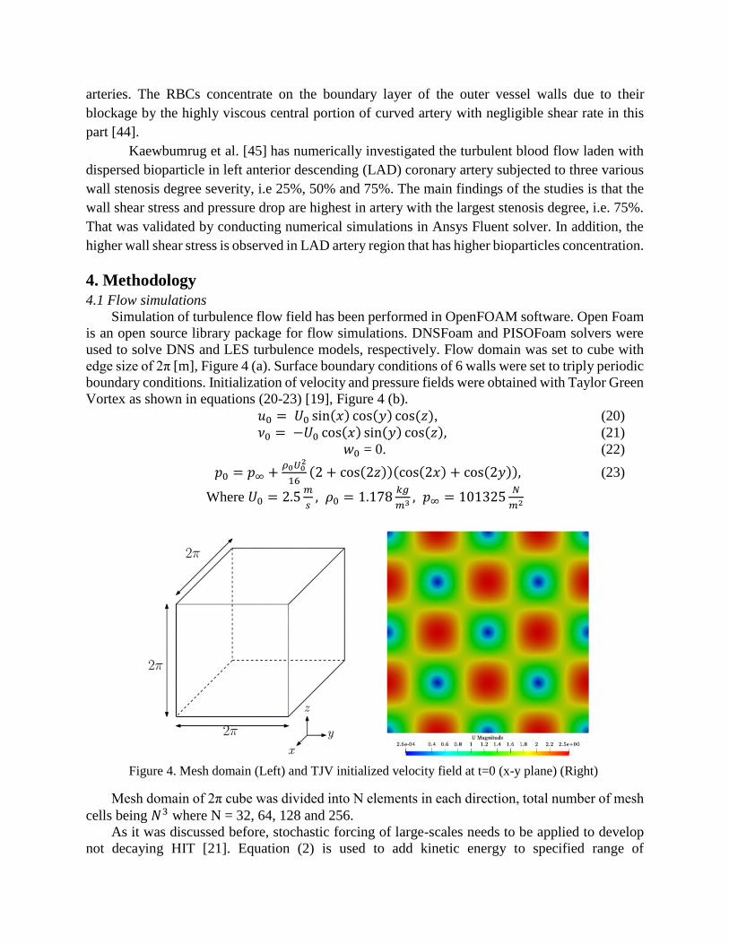
used to solve DNS and LES turbulence models, respectively. Flow domain was set to cube with

edge size of 2π [m], Figure 4 (a). Surface boundary conditions of 6 walls were set to triply periodic

boundary conditions. Initialization of velocity and pressure fields were obtained with Taylor Green

Vortex as shown in equations (20-23) [19], Figure 4 (b).

𝑢0 = 𝑈0 sin(𝑥) cos(𝑦) cos (𝑧), (20)

𝜈0 = −𝑈0 cos(𝑥) sin(𝑦) cos(𝑧), (21)

𝑤0 = 0. (22)

𝑝0 = 𝑝∞ +𝜌0𝑈0

2

16(2 + cos(2𝑧))(cos(2𝑥) + cos(2𝑦)), (23)

Where 𝑈0 = 2.5𝑚

𝑠, 𝜌0 = 1.178

𝑘𝑔

𝑚3 , 𝑝∞ = 101325𝑁

𝑚2

Figure 4. Mesh domain (Left) and TJV initialized velocity field at t=0 (x-y plane) (Right)

Mesh domain of 2π cube was divided into N elements in each direction, total number of mesh

cells being 𝑁3 where N = 32, 64, 128 and 256.

As it was discussed before, stochastic forcing of large-scales needs to be applied to develop

not decaying HIT [21]. Equation (2) is used to add kinetic energy to specified range of

wavenumbers 𝑘𝜖[0, √8 ] which was used as forcing range of wavenumber in works of [20], [24]

and [21]. Values of scales “k” are located in range of 𝑘𝑙𝑜𝑤 =2𝜋

𝐿 and 𝑘𝑚𝑎𝑥 =

√2

3𝑘0𝑁 .

All simulations are performed with 𝑑𝑡 = 0.005 𝑠. Pressure field and velocity data field was

recorded with an intervals of 0.5 s of flow simulation time. Volume averaged velocity fluctuations

are monitored with Equation (15). Integral length scale has been calculated by equation suggested

by [21] as shown below (14)

𝐿 =𝜋

2𝑈′2∫ 𝑘−1𝐸(𝑘)𝑑𝑘

𝑘𝑚𝑎𝑥

0 (24)

𝑈′ 𝑖s the RMS value of volume averaged velocity fluctuations.

𝑈′ = √1

3(⟨𝑈′𝑥𝑥⟩ + ⟨𝑈′𝑦𝑦⟩ + ⟨𝑈′𝑧𝑧⟩) (25)

Average rate of energy dissipation can be estimated by (26)

𝜖 =𝑈′3

𝐿 (26)

Taylor microscale is estimated with (27)

𝜆 = √15𝜈

𝜖 (27)

Taylor scale Reynolds Number is estimated as follows (28)

𝑅𝑒𝜆 =𝑈′𝜆

𝜈 (28)

Kolmogorov time scale is evaluated with (29) and large eddy turnover time is estimated with (30)

𝑡𝜂 = (𝜈

𝜖)

1

2 (29)

𝑇𝑒 =𝐿

𝑈′ (30)

Main flow parameters of flow for evaluation of HIT will be U’,𝑅𝑒𝜆, 𝐿 and 𝑡𝜂.

In addition, parallelization of mesh domain needs to be implemented to decrease the

computational domain. Simple mesh decompositions methods where domain of study is divided

into sliced sections are shown in Figure 5 (a). Due to presence of Fourier space in stochastic forcing

term which require equal number of elements in each coordinate system, it is not possible to apply

simple sliced mesh decomposition method.

Figure 5. Simple decomposition (Left) and suggested decomposition (Right)

It was decided to divide the mesh domain into equal size cubes with number of element in each

direction being half of initial grid points (N).

4.2 Simulation of particle phase

The results obtained from the flow simulation are then used for simulation of particle phase. From

the energy spectrum graph, it was determined that turbulence becomes statistically stationary after

about 40 seconds. The velocity field from the flow simulations after the fortieth second was used

for calculation of particles’ trajectories. The simulations were performed in Matlab and CFDEM.

Simulations in MATLAB

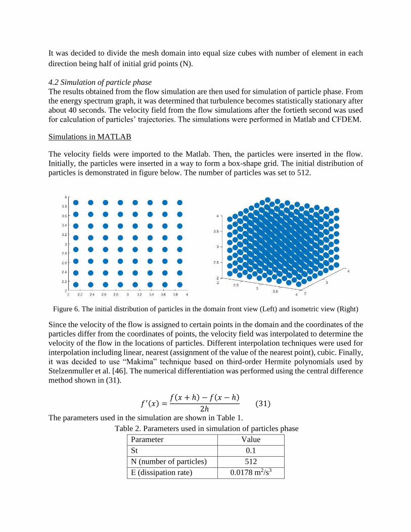
The velocity fields were imported to the Matlab. Then, the particles were inserted in the flow.

Initially, the particles were inserted in a way to form a box-shape grid. The initial distribution of

particles is demonstrated in figure below. The number of particles was set to 512.

Figure 6. The initial distribution of particles in the domain front view (Left) and isometric view (Right)

Since the velocity of the flow is assigned to certain points in the domain and the coordinates of the

particles differ from the coordinates of points, the velocity field was interpolated to determine the

velocity of the flow in the locations of particles. Different interpolation techniques were used for

interpolation including linear, nearest (assignment of the value of the nearest point), cubic. Finally,

it was decided to use “Makima” technique based on third-order Hermite polynomials used by

Stelzenmuller et al. [46]. The numerical differentiation was performed using the central difference

method shown in (31).

𝑓′(𝑥) =𝑓(𝑥 + ℎ) − 𝑓(𝑥 − ℎ)

2ℎ (31)

The parameters used in the simulation are shown in Table 1.

Table 2. Parameters used in simulation of particles phase

Parameter Value

St 0.1

N (number of particles) 512

Ε (dissipation rate) 0.0178 m2/s3

ν 1.7*10-5 kg/(m·s)

𝜏𝜂 3.09*10-3

𝜏𝑝 3.09*10-4

Then Maxey-Riley equation was used for calculation of particles’ trajectories. The initial velocity

of inertial particles were set to zero. The obtained results were plotted in the domain. However,

the simulations in Matlab revealed several constraints. The boundary conditions for the simulation

were not periodic, since the domain was presented as a cube with walls. The results showed that

the majority of particles tend to leave the flow domain. However, when they left the domain the

interpolation could not be performed for such particles – the interpolation of velocity field showed

error. Moreover, the particles in the simulations were presented as points rather than spheres. This

representation of particles was not realistic. Finally, the simulations in Matlab were

computationally expensive. This problem was not significant for small mesh grids, however, the

increase of mesh grid size led to abrupt increase of computational time. Therefore, it was decided

to perform the simulations of particle phase in CFDEM software.

Simulations in CFDEM

CFDEM is an open-source software, which combines OpenFOAM software and LIGGGHTS.

OpenFOAM is used for simulation of flow, whereas LIGGGHTS is based on LAMMPS and used

for simulation of particle phase. CFDEM does not include numerous libraries from OpenFOAM

such as forcing term library and dnsFOAM solver. Meaning that it only allows simulating decaying

turbulence with particles inside. The LES simulation was used to solve decaying turbulence with

particles. Initially, the inertial particles were distributed randomly in the flow domain. The

parameters of the turbulent flow were the same as for the homogeneous isotropic turbulence.

Table 3. The parameters used for decaying turbulence with particles in CFDEM

Parameter Value

a 30μm

ε 0.0178 m2/s3

N 1000

ν 1.7*10-5 kg/(m·s)

ρf 1.178 kg/m3

ρd 1000 kg/m3

𝜏𝜂 3.09*10-3

St 0.323

𝜏𝑝 9.981*10-4

4.3 Particles’ pair dispersion

The data was threated via Matlab software. The experimental data, which was considered, was

recieved from experiment, conducted by Sumbekova et al. [47]. The main aim of the experiment

was to observe the clustering phenomenon during strong turbulence. The experiment, conducted

in wind tunnel, investigated the movement of water droplets, injected through its test section. The

tracking of inertial particles occurred via illumination of wind tunnel by vertical laser sheet. The

position of each particle was recorded on series of images, captured by high-speed camera. The

one recording lasted 3.27 seconds with acquisition rate of 2600 frames per second. 19 cases with

different Stokes and Taylor scale Reynolds numbers were considered during the experiment and

for each case 20 movies were recorded. In total, it results to 380 movies, which were analyzed.

The variation of Stokes number occurred through the change in injected water droplets’ diameter

and their flow rate, whereas the Reynolds number was changed via increase in wind velocity in

wind tunnel. The wind velocities which were set during the experiment were 2.5 m/s, 5 m/s, 7.5

m/s and 10 m/s. All considered values of parameters and corresponding to them values of

Kolmogorov time and length scales are represented on Table 4.

Table 4. The values of parameters. [9]

𝑈(m/s) 𝐷 (mm) 𝐹𝑤𝑎𝑡𝑒𝑟 (L/min) 𝜂 (µm) 𝜏𝜂 (s) 𝑆𝑡𝐷𝑚𝑎𝑥 𝑅𝑒𝜆

2.5 0.3 0.8 431 0.011 0.3 200

5.0 0.3 0.8 250 0.004 0.7 300

7.5 0.3 0.8 162 0.002 1 400

10.0 0.3 0.8 114 0.001 5 490

2.5 0.3 1.2 429 0.011 0.1 240

5.0 0.3 1.2 255 0.004 0.5 350

7.5 0.3 1.2 174 0.002 0.9 390

10.0 0.3 1.2 118 0.001 2.7 470

2.5 0.4 1.9 439 0.012 0.3 240

5.0 0.4 1.9 260 0.004 1.4 290

7.5 0.4 1.9 174 0.002 1.6 420

10.0 0.4 1.9 121 0.001 2.8 480

5.0 0.4 1.43 252 0.004 0.5 300

7.5 0.4 1.43 166 0.002 1.4 420

10.0 0.4 1.43 118 0.001 2.7 480

2.5 0.5 1.9 442 0.012 0.1 200

5.0 0.5 1.9 249 0.004 0.8 290

7.5 0.5 1.9 168 0.002 2.3 400

10.0 0.5 1.9 120 0.001 3.5 480

The detected positions of the water droplets were processed and the coordinates of particles

on each image were determined. The Matlab code sorted inertial particles by all possible

combinations of pairs. For each pair the square of distance between the particles was calculated.

Mean square dispersion and its evolution with time for each set of measurements were obtained.

The mean square separation was normalized by the dissipative scale 𝜂2 , whereas time was

normalized by the dissipative time scale 𝜏𝜂. The number of graphs, representing the dependence

of mean square dispersion on normalized time, was constructed.

4.4.1 Simulations of particles (blood clots) in arteries

The numerical simulations of two-phase flows in coronary arteries have been performed via Ansys

Fluent finite-element solver. The Ansys CFD software enables to discretize and numerically solve

continuity and Navier-Stokes equations. The blood was treated as non-Newtonian, incompressible,

steady fluid with density 1060 𝑘𝑔/𝑚3 and dynamic viscosity of 0.0035 𝑚2/𝑠. The blood clots

were modelled as spherical particles with density 1100 𝑘𝑔/𝑚3 and dimeter of 2.5 mm. (Romero,

2013). The artery wall density was set to 1160 𝑘𝑔/𝑚3. After the 3D geometry has been imported

in Ansys solver, the mesh was generated. In order to validate the independence of results from the

grid size, the mesh independence study has been conducted, which is described in the following

section. The blood phase and particle phase, represented by blood clots, were resolved using one-

way coupled Euler-Lagrange approach. As Indicated in Table 1, the flow regime was laminar

throughout the CHN03 artery. In the ‘Setup’ mode, the ‘Viscous’ model has been chosen. The

thermodynamic properties of blood, clots and artery wall, i.e. density and viscosity, has been typed

in ‘Materials’ section. In ‘Cell Zone Conditions’ mode, the fluid type has been changed from solid

to liquid. In the ‘Boundary Conditions’ windows, the pressure and mass flow rate were assigned

for inlet and outlets, respectively. The mass flow rate at the outlets has been calculated by

multiplying blood density by the volume flow rate. In the ‘Solutions Methods’ mode, the

‘Coupled’ scheme has been selected for pressure-velocity coupling. The ‘Least Squares Cell

Based’ gradient has been selected for spatial discretization. The pressure and momentum equations

were discretized with ‘Second Order’ and ‘Second Order Upwind’ Scheme. The Discrete Phase

Model has been tuned on to inject particles at the inlet and track their motion within artery. The

particle phase was tracked in a steady mode. Initially, 100 particles were injected at the inlet of

vessel of CHN03 model. Firstly, the single blood flow phase was simulated with 1000 iterations

to attain fully developed entrance region in laminar flow field and reach the statistical convergence

of the velocity profiles. Afterwards, the two-phase flow field was injected until further

convergence within the defined tolerance. In total, 8000 iterations were performed for CHN03

model. The convergence criterion was set to residual values of 10−6 for each parameter, i.e.

continuity and x, y, z velocity equations.

4.4.2 Mesh convergence study

The mesh convergence study has been conducted for CHN03 model in order to validate the

independence of results on the variation of element size. The computational domain of the artery

3D geometry has been discretized into finite elements to ensure accurate numerical results. The

mesh of tetrahedral structure has been assigned for the curved vessel geometry. Table 5 illustrates

the variation of parameters, i.e. average and maximum velocities and pressure, against number of

mesh nodes and elements variation. The parameters that were selected for the variation against

number of elements are maximum pressure and maximum velocity. Table 6 illustrates that the

percentage error of maximum pressure and velocity between consecutive iterations is equal to

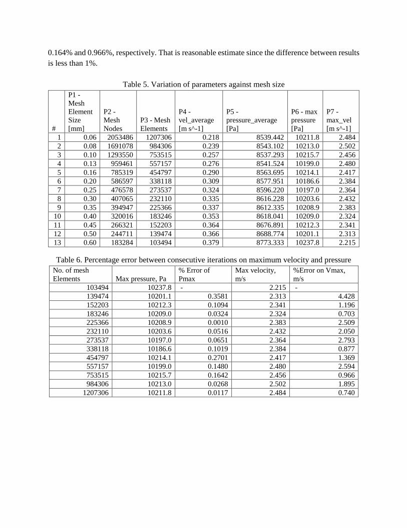
0.164% and 0.966%, respectively. That is reasonable estimate since the difference between results

is less than 1%.

Table 5. Variation of parameters against mesh size

#

P1 -

Mesh

Element

Size

[mm]

P2 -

Mesh

Nodes

P3 - Mesh

Elements

P4 -

vel_average

[m s^-1]

P5 -

pressure_average

[Pa]

P6 - max

pressure

[Pa]

P7 -

max_vel

[m s^-1]

1 0.06 2053486 1207306 0.218 8539.442 10211.8 2.484

2 0.08 1691078 984306 0.239 8543.102 10213.0 2.502

3 0.10 1293550 753515 0.257 8537.293 10215.7 2.456

4 0.13 959461 557157 0.276 8541.524 10199.0 2.480

5 0.16 785319 454797 0.290 8563.695 10214.1 2.417

6 0.20 586597 338118 0.309 8577.951 10186.6 2.384

7 0.25 476578 273537 0.324 8596.220 10197.0 2.364

8 0.30 407065 232110 0.335 8616.228 10203.6 2.432

9 0.35 394947 225366 0.337 8612.335 10208.9 2.383

10 0.40 320016 183246 0.353 8618.041 10209.0 2.324

11 0.45 266321 152203 0.364 8676.891 10212.3 2.341

12 0.50 244711 139474 0.366 8688.774 10201.1 2.313

13 0.60 183284 103494 0.379 8773.333 10237.8 2.215

Table 6. Percentage error between consecutive iterations on maximum velocity and pressure

No. of mesh

Elements Max pressure, Pa

% Error of

Pmax

Max velocity,

m/s

%Error on Vmax,

m/s

103494 10237.8 - 2.215 -

139474 10201.1 0.3581 2.313 4.428

152203 10212.3 0.1094 2.341 1.196

183246 10209.0 0.0324 2.324 0.703

225366 10208.9 0.0010 2.383 2.509

232110 10203.6 0.0516 2.432 2.050

273537 10197.0 0.0651 2.364 2.793

338118 10186.6 0.1019 2.384 0.877

454797 10214.1 0.2701 2.417 1.369

557157 10199.0 0.1480 2.480 2.594

753515 10215.7 0.1642 2.456 0.966

984306 10213.0 0.0268 2.502 1.895

1207306 10211.8 0.0117 2.484 0.740

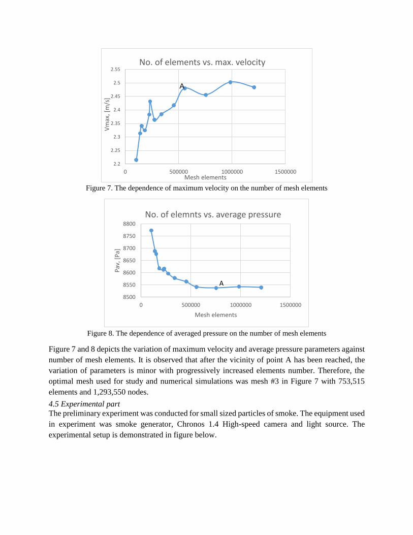
Figure 7. The dependence of maximum velocity on the number of mesh elements

Figure 8. The dependence of averaged pressure on the number of mesh elements

Figure 7 and 8 depicts the variation of maximum velocity and average pressure parameters against

number of mesh elements. It is observed that after the vicinity of point A has been reached, the

variation of parameters is minor with progressively increased elements number. Therefore, the

optimal mesh used for study and numerical simulations was mesh #3 in Figure 7 with 753,515

elements and 1,293,550 nodes.

4.5 Experimental part

The preliminary experiment was conducted for small sized particles of smoke. The equipment used

in experiment was smoke generator, Chronos 1.4 High-speed camera and light source. The

experimental setup is demonstrated in figure below.

2.2

2.25

2.3

2.35

2.4

2.45

2.5

2.55

0 500000 1000000 1500000

Vm

ax, [

m/s

]

Mesh elements

No. of elements vs. max. velocity

8500

8550

8600

8650

8700

8750

8800

0 500000 1000000 1500000

Pav

, [P

a]

Mesh elements

No. of elemnts vs. average pressure

A

A

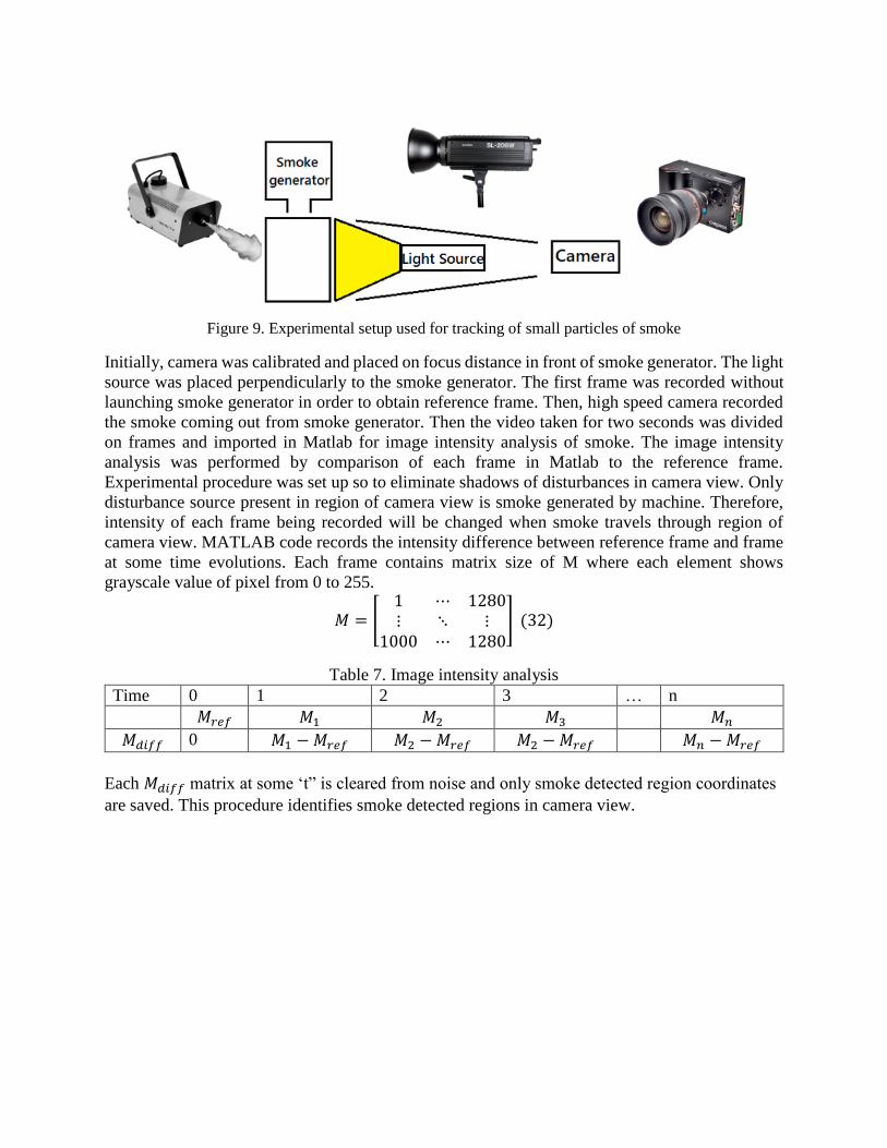
Figure 9. Experimental setup used for tracking of small particles of smoke

Initially, camera was calibrated and placed on focus distance in front of smoke generator. The light

source was placed perpendicularly to the smoke generator. The first frame was recorded without

launching smoke generator in order to obtain reference frame. Then, high speed camera recorded

the smoke coming out from smoke generator. Then the video taken for two seconds was divided

on frames and imported in Matlab for image intensity analysis of smoke. The image intensity

analysis was performed by comparison of each frame in Matlab to the reference frame.

Experimental procedure was set up so to eliminate shadows of disturbances in camera view. Only

disturbance source present in region of camera view is smoke generated by machine. Therefore,

intensity of each frame being recorded will be changed when smoke travels through region of

camera view. MATLAB code records the intensity difference between reference frame and frame

at some time evolutions. Each frame contains matrix size of M where each element shows

grayscale value of pixel from 0 to 255.

𝑀 = [1 ⋯ 1280⋮ ⋱ ⋮

1000 ⋯ 1280] (32)

Table 7. Image intensity analysis

Time 0 1 2 3 … n

𝑀𝑟𝑒𝑓 𝑀1 𝑀2 𝑀3 𝑀𝑛

𝑀𝑑𝑖𝑓𝑓 0 𝑀1 − 𝑀𝑟𝑒𝑓 𝑀2 − 𝑀𝑟𝑒𝑓 𝑀2 − 𝑀𝑟𝑒𝑓 𝑀𝑛 − 𝑀𝑟𝑒𝑓

Each 𝑀𝑑𝑖𝑓𝑓 matrix at some ‘t” is cleared from noise and only smoke detected region coordinates

are saved. This procedure identifies smoke detected regions in camera view.

5. Results and discussion

5.1 Simulation of flow

Figure 10 TJV initialized velocity field at time =1s (Left) and Velocity field at time = 26 s, N=128 (Right)

TGV initialized field with velocity amplitude of 2 m/s will decay with time evolution.

Figure 10 shows velocity field at the t = 1s of simulation from LES solver for mesh size of N=256

(𝜎=2, 𝛼=50). Figure 10 shows velocity of HIT at t = 26 s where fluctuations of velocity field are

clearly seen. These velocity fluctuations will be estimated with equation (25) and energy present

in each scale will be evaluated with Energy spectrum plots, Figure 13.

Figure 11 Mesh variation study for LES and DNS solvers (Left) time evolution of U’ for different values

of acceleration variance, N=256 (LES) solver (Right)

It is important to study the effect of mesh resolution on flow characteristics of simulated

HIT. Mesh value of studied domain was increased gradually from N=32 until N=256. U’ value

was evaluated at the end time of 64s. Minimum difference of 9.0%, between consecutive values

of U’ for each N change, was achieved with LES solver Figure 11. DNS solver also have shown

similar performance on mesh size variation, Figure 11. Minimum value of U’ keeps decreasing

with increasing mesh size for DNS solution. This trend is explained with the fact that DNS is better

at resolving small scales.

It is possible to increase mesh size of N to 512. Since solution was performed on a single

core, intolerable increase of computational time for mesh generation at N=512 was observed.

Therefore, N=256 was taken as best grid resolution for rest of calculations.

As it was discussed before, forcing term is added to achieve statistically stationary HIT.

Different values of 𝜎 were simulated with LES solver for N=256. Increase in peak value of U’ at

turbulence generation region is observed in Figure 11. Results of this simulations show that it is

possible to control values velocity fluctuations and energy dissipation rate (they are related with

26) for HIT by changing the value of acceleration variance (𝜎).

Figure 12. Energy spectrum evolution with time (Left) and energy spectrum for different grid resolution

after turbulence generation is achieved (Right)

Energy spectrum is one of the main characteristics to evaluate properties of not decaying HIT.

Figure 12 (Left) depicts that energy spectrum did not change with time evolution. It is supported

with Figure 12 (Right) where turbulence generation is achieved approximately at t=20 s. Therefore,

it is possible to state that not decaying HIT condition is expected after this time point.

The slope of energy spectrum should be close to the curve of 1.62𝑘−5/4[20], Figure 1. It

shows whether small scales are fully resolved or not. The curvature obtained by [20] cannot be

fully followed since [20] has used different forcing values and forcing time in their simulations.

Figure 12 (Left) shows that scales in range of 𝑘 ∈ [0,22] are fully resolved. If slope is checked

after this range, the deviation from expected slope can be noticed. Figure 12 (Right) depicts energy

spectrum of different grid resolutions at t = 20s. It is evident from the graph that N=256

performance is better than other two. Greater mesh resolution will capture a greater amount of

small scale fluctuations. Range of wavenumber that are fully resolved is bigger for larger N as it

was expected.

Figure 13. Estimated Length Scale variation with time after turbulence generation region (t> 20s) (b)

Energy spectrum from LES and DNS solvers

Length Scale is estimated at each time step value using (24) and obtained results are shown

in Figure 13 (Left). Moderate level of fluctuations is observed for length values over time. It may

occur due to the presence of acceleration variance in forcing term which is based on noise

producing equations. In addition, increasing trend in length scale values is observed. It can be

explained with Figure 11 (Left) where U’ value decreases over time which results in larger length

scale values as it is stated in equation (24).

LES and DNS solver performances differ in smaller scales. DNS solver can resolve smaller

scales from its definition. It can be illustrated in Figure 13 (Right) where energy spectrum curve

for DNS solver for N=128 and N=256 keeps its slope close to expected curvature of energy

spectrum suggested by [20].

Figure 14. Effect of forcing time on U’ (Left) and effect of forcing time on U’ zoomed to smaller forcing

time legends (Right)

Forcing time is crucial when evaluating the HIT parameters [24]. Some studies have found

relation between forcing time scale and large eddy turnover time as it was noted before [25]. There

are should be limit when forcing time will not have significant effect on HIT parameters like U’.

Figure 14 (Left) shows that 𝛼 = {80, 125, 150} are closely located which implies presence of

smaller variation between U’ values between the lines. Figure 14 (Right) illustrates that smaller

difference is present between U’ values for 𝛼 = {125, 150}.

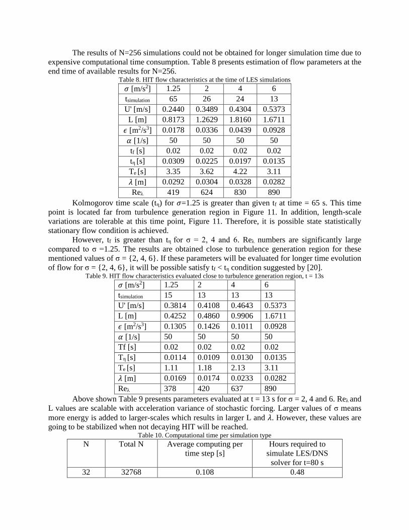
The results of N=256 simulations could not be obtained for longer simulation time due to

expensive computational time consumption. Table 8 presents estimation of flow parameters at the

end time of available results for N=256. Table 8. HIT flow characteristics at the time of LES simulations

𝜎 [m/s2] 1.25 2 4 6

tsimulation 65 26 24 13

U' [m/s] 0.2440 0.3489 0.4304 0.5373

L [m] 0.8173 1.2629 1.8160 1.6711

𝜖 [m2/s3] 0.0178 0.0336 0.0439 0.0928

𝛼 [1/s] 50 50 50 50

tf [s] 0.02 0.02 0.02 0.02

tη [s] 0.0309 0.0225 0.0197 0.0135

Te [s] 3.35 3.62 4.22 3.11

𝜆 [m] 0.0292 0.0304 0.0328 0.0282

Reλ 419 624 830 890

Kolmogorov time scale (tη) for 𝜎=1.25 is greater than given tf at time = 65 s. This time

point is located far from turbulence generation region in Figure 11. In addition, length-scale

variations are tolerable at this time point, Figure 11. Therefore, it is possible state statistically

stationary flow condition is achieved.

However, tf is greater than tη for σ = 2, 4 and 6. Reλ numbers are significantly large

compared to σ =1.25. The results are obtained close to turbulence generation region for these

mentioned values of σ = {2, 4, 6}. If these parameters will be evaluated for longer time evolution

of flow for σ = {2, 4, 6}, it will be possible satisfy tf < tη condition suggested by [20]. Table 9. HIT flow characteristics evaluated close to turbulence generation region, t = 13s

𝜎 [m/s2] 1.25 2 4 6

tsimulation 15 13 13 13

U' [m/s] 0.3814 0.4108 0.4643 0.5373

L [m] 0.4252 0.4860 0.9906 1.6711

𝜖 [m2/s3] 0.1305 0.1426 0.1011 0.0928

𝛼 [1/s] 50 50 50 50

Tf [s] 0.02 0.02 0.02 0.02

Tη [s] 0.0114 0.0109 0.0130 0.0135

Te [s] 1.11 1.18 2.13 3.11

𝜆 [m] 0.0169 0.0174 0.0233 0.0282

Reλ 378 420 637 890

Above shown Table 9 presents parameters evaluated at t = 13 s for σ = 2, 4 and 6. Reλ and

L values are scalable with acceleration variance of stochastic forcing. Larger values of σ means

more energy is added to larger-scales which results in larger L and 𝜆. However, these values are

going to be stabilized when not decaying HIT will be reached. Table 10. Computational time per simulation type

N Total N Average computing per

time step [s]

Hours required to

simulate LES/DNS

solver for t=80 s

32 32768 0.108 0.48

64 262144 2 8.89

128 2097152 20.7 92.00

256 16777216 325.3 1445.78

As above shown Table 10 illustrates computation time required for N=256 is significantly

large. Therefore, parallelization parallel computing approaches need to be implemented. Mesh

domain decomposition method is suggested for this kind of simulation. Suggested mesh

decomposition method in Figure 5 has been tested for N =64 and128 with OpenFOAM DNS

solver. They were compared to single core solved simulation results and obtained values of U’

were identical, Figure 15

Figure 15. Parallel and single core simulation results

5.2 Simulation of particle phase

5.2.1 MATLAB Software

The results obtained in Matlab are shown in figure below.

Figure 16. The distribution of particles in the space after (A) t=0.01s, (B) t=0.02s, (C) t=0.03s, (D)

t=0.04s

The results obtained from MATLAB showed that the majority of particles leave the domain. For

the particles, which left the domain, the interpolation was done incorrectly. The velocities of such

particles were too high, therefore, their location in 0.04 seconds reached 80 meters from the initial

positions. It can be seen from Figure 9 (D), that the particles are distributed in the area [-70; 70] in

x-axis and [-50; 80] in y-axis. The dynamics of particles could not be investigated, since the

particles were out of the flow domain and were not exposed to the influence of the turbulence.

Therefore, it was decided to perform the simulations of particles phase in CFDEM software.

5.2.2 CFDEM

The results obtained for pressure and velocity fields in CFDEM are shown in figures below. The

initial distribution of particles in the domain is shown in figure 10.

Figure 17. The initial distribution of particles in XY plane (Left) and XZ plane (Right)

Figure 18. Pressure field obtained from decaying turbulent simulations in CFDEM. T = 0s (Left), T =

0.05s (Right)

Figure 19. Velocity field obtained from decaying turbulent simulations in CFDEM. T = 0s (Left),

T = 0.05s (Right)

It can be seen from Figures 11 and 12, that the turbulent flow is decaying with time. Since the

boundary conditions were set to periodic, particles did not leave the flow domain and were moving

in turbulent flow. However, the particle phase was simulated for only 0.05s, since the turbulent

decayed.

5.3 Pair dispersion of inertial particles in turbulent flow

Figure 19. The evolution of mean square separation with time for all cases

The Figure 19 represents the evolution of normalized value of mean square separation with

normalized time. The Figure 19 includes the results, obtained for the inertial particles for all

considered cases. Figure 20-23 show same graphs for each value of wind velocity separately. All

pairs of particles, initial distance between which was not exceed 100𝜂, were considered during

construction of graph. All graphs, made for the inertial particles, possess same feature. Normalized

mean square dispersion does not change significantly with time during first decade. In the second

half of graphs, the strong fluctuations, which are result of scarcity of experimental data, are

observed. Another important point is that the higher velocity of the wind corresponds to greater

value of initial separation between particles. Hence, there is correlation between velocity of tracers

and initial separation value of inertial particles.

Figure 20. The evolution of mean square separation with time for wind veclocity of 2.5 m/s

Figure 21. The evolution of mean square separation with time for wind velocity of 5 m/s

Figure 22. The evolution of mean square separation with time for wind veclocity of 7.5 m/s

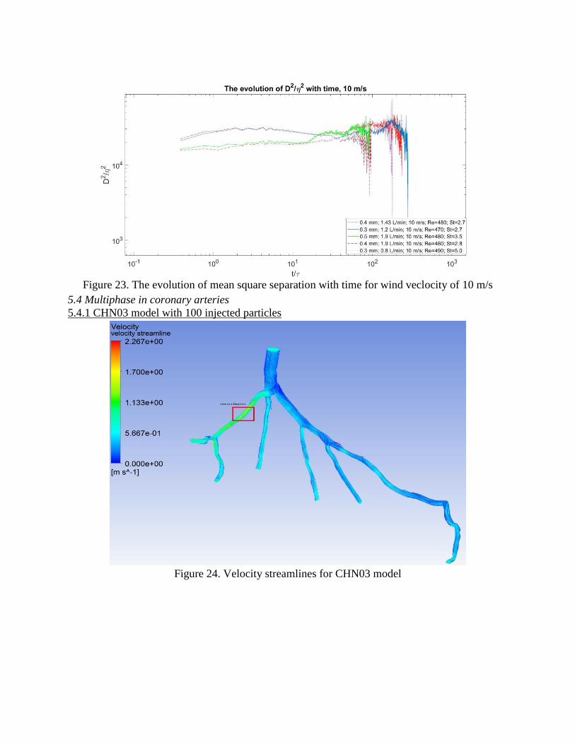
Figure 23. The evolution of mean square separation with time for wind veclocity of 10 m/s

5.4 Multiphase in coronary arteries

5.4.1 CHN03 model with 100 injected particles

Figure 24. Velocity streamlines for CHN03 model

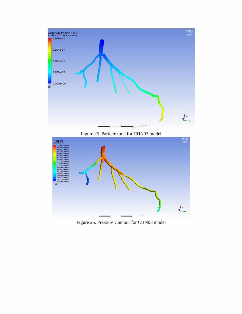
Figure 25. Particle time for CHN03 model

Figure 26. Pressure Contour for CHN03 model

Figure 27. Wall Shear Stress for CHN03

Figure 28. PDF distribution of particles (Left) x-velocity; (Central) y-velocity; (Right) z-velocity

Figure 29. PDF distribution of flow (Left) x-velocity; (Central) y-velocity; (Right) z-velocity

5.4.2 CHN03 model with 1000 injected particles

Figure 30. Velocity streamlines for CHN03 model (1000 particles)

Figure 31. Particle time for CHN03 model (1000 particles)

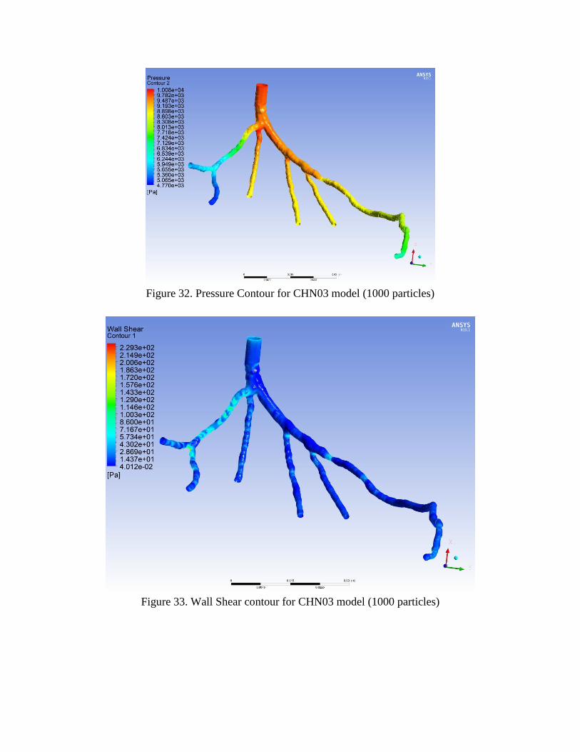
Figure 32. Pressure Contour for CHN03 model (1000 particles)

Figure 33. Wall Shear contour for CHN03 model (1000 particles)

a) b)

Figure 34. PDF distribution of particles a) x-velocity; b) y-velocity

5.4.3 Numerical simulations for CT14 model

Figure 35. Velocity streamline for CT14 model

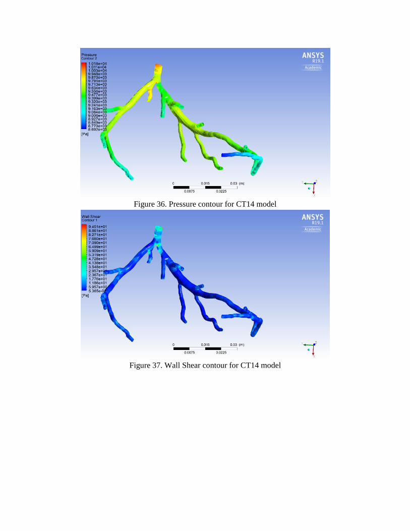
Figure 36. Pressure contour for CT14 model

Figure 37. Wall Shear contour for CT14 model

Figure 38. Particle time CT14 model

5.4.4 Numerical simulations for CT209 model

Figure 39. Velocity streamlines for CT209 model

Figure 40. Wall Shear for CT209 model

Figure 41. Particle time for CT209 model

5.4.5 Numerical simulations for CHN13 model

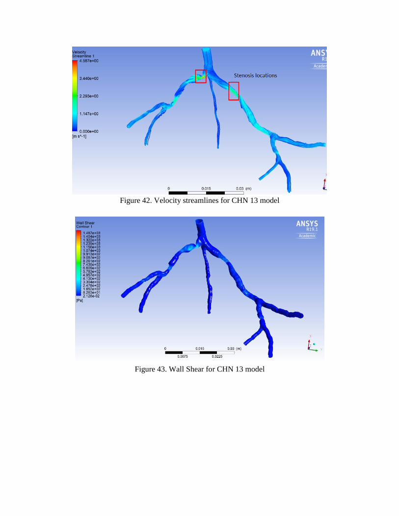
Figure 42. Velocity streamlines for CHN 13 model

Figure 43. Wall Shear for CHN 13 model

Figure 44. Particle time for CHN13 model

The numerical simulations have been performed in Ansys Fluent finite-element solver. For each

model, the results have been post processed in Ansys CFD Post. The results that have been

obtained for the four artery models, i.e. CHN03, CT14, CT209 and CHN13, are velocity

streamlines, particle time, pressure contours and wall shear stress. Figures 24-27 illustrate

simulation results for CHN03 artery model with 100 particles injected at the inlet. The velocity

streamlines results for all artery models indicate the local velocity values at the particular regions

of the branches. The locations where the artery cross-section narrows corresponds to the maximum

values of velocity. Under the steady flow regime of blood, the decrease in area of the vessel wall

implies higher velocity rate. That is true by continuity equation. In addition, the narrowed artery

wall corresponds to the region of plaque accumulation, i.e. stenosis formation. Consequently, the

stenotic region is formed at the branches, where the velocity flow is maximum. In Figure 24, the

maximum velocity of 2.27 m/s is observed in the leftmost daughter branch. The red square boxes

indicate the region of stenosis formation. The particle time results indicate the total time required

for the particle to reach the distinct region of outlet branches. In the case of CHN03 model, the

maximum particle time (0.387 s) is observed for the longest branch, located at the rightmost side.

The pressure contour plots enable to estimate static pressure values within artery as well as

pressure drop across the branch. For the all models considered, the wall shear stress reaches highest

values at the stenotic regions. The particle track data contained information about the particles

position and velocity components in three spatial coordinates (x, y, z) at each residence time value.

The PDF distributions of particles’ three velocity components have been plotted in MATLAB

software against number of bin elements, represented by heights of individual rectangles that are

equally distributed along horizontal axes. The number of bins corresponds to the total number of

rectangles. The PDF distribution graphs of the particle velocities follow Gaussian distribution (Fig.

28). That implies that velocities of particles have settled within statistical convergence. Fig. 29

depicts histogram of velocity distributions of the single flow against number of bin counts.

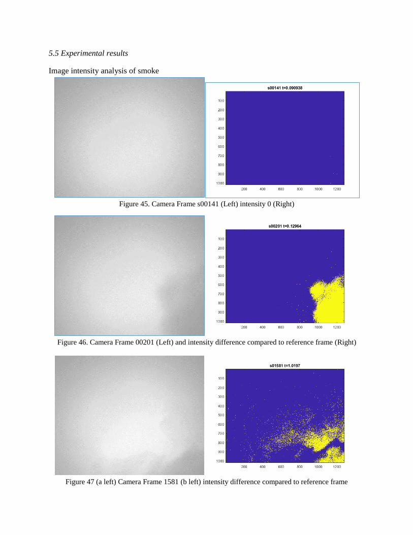
5.5 Experimental results

Image intensity analysis of smoke

Figure 45. Camera Frame s00141 (Left) intensity 0 (Right)

Figure 46. Camera Frame 00201 (Left) and intensity difference compared to reference frame (Right)

Figure 47 (a left) Camera Frame 1581 (b left) intensity difference compared to reference frame

Figure 45, 46 and 47 illustrates the actual frame from camera and MATLAB intensity

analysis results. Smoke traveling region in 2D plane was detected per each frame. Comparison can

be made with visual frame on the left and analyzed frame on the right. However, noises are present

in results of intensity difference frames. In addition, effect of light source is sensible in intensity

graphs.

Movement of smoke could be tracked with this preliminary code. However, it is not

possible to measure the velocity of the flow and smoke cloud sizes cannot be detected from frames.

Therefore, it is suggested to perform experiment with water droplet injection.

6. Conclusion In the first part of the capstone project, LES and DNS methods have been implemented to

generate statistically stationary HIT field. In order to achieve statistically stationary HIT,

stochastic forcing term developed has been successfully added to the OpenFOAM solvers. Series

of simulations were performed with different mesh sizes to study the effect of meshing to volume

averaged velocity fluctuations. Grid size of N=256 have shown best performance when flow

parameters of the simulations were analyzed. It was expected since small scales fully resolved at

finer mesh sizes. Effect forcing time constant 𝛼 on U’ has been studied. The condition 𝑡𝑓 < 𝑡𝜂

when energy dissipation rate remains constant (not decaying turbulence) has been achieved at

simulation time of t=65s for N=256. In addition, fluctuations of large-scales values over time were

increasing due to decrease of U’. However, slope of U’ decrease tends to zero resulting in not

decaying flow. The results obtained from DNS simulations showed that an increase of number of

mesh elements led to smaller velocity fluctuations due to the better resolution of smaller scales.

Statistically stationary HIT could not be fully achieved for all variation of 𝛼 in this work

due to expensive computational time. Nevertheless, it was found that it is possible to control energy

production region and U’ magnitude with acceleration variance 𝜎. Energy spectrum curve for

scales present in HIT was obtained for N=256. Slope of energy spectrum follow suggested slope

of 1. 62𝑘−5/4. Parallel computing approach with 8 cores (instead of single core) was developed

for DNS solver that showed identical results for U’ magnitude. Code development of parallel

solution will be considered in future work to increase computational efficiency of simulations.

The simulations of particle phase were performed in Matlab and CFDEM. The results

obtained from Matlab revealed several constraints of the solver. The interpolation of the velocity

field was incorrect for the particles which left the flow domain. Additionally, in the simulations,

the particles were presented as points rather than spheres. This made the physical model

unrealistic. Finally, the simulations in Matlab were computationally expensive. The computational

expensiveness was not a problem for a small number of mesh elements, however, for the

simulations of N=256, it would be significantly. Then the simulations were performed in CFDEM

software. Since the solver does not include forcing terms, the HIT was not reached. The decaying

turbulence with particle phase was simulated. However, in order to investigate the dynamics of the

particles, the HIT should be used for the flow phase. There are two possible solutions to this issue:

write the libraries containing DNS solver and forcing term or change the solver in CFDEM to

make it take the results from OpenFOAM simulations. It was decided to choose the second

alternative since the results for flow simulations from OpenFOAM were already obtained. The

new simulations of the flow domain will take a considerable amount of time.

The change of mean square separation with time was investigated and was represented on

graphs with normalized scales. Firstly, it was concluded, that the higher velocity of the wind

corresponds to greater value of normalized initial separation between particles. Also, it was pointed

out that the graphs for the different cases possess same features. On each graph two different parts

were distinguished. The first part of graph is characterized by insignificant change of normalized

mean square dispersion with time until the first decade, whereas the second part contains a lot of

fluctuations. The fluctuations were caused by the limitations in tracking of the particles, which

traveled long distances or traveled out from the tracking range. The scarcity of the long tracks

leads to the fact that statistical convergence of results is not achieved on the second part of the

graphs. To increase the long tracks’ number it is required to apply cameras with higher acquisition

rate during experiment. This allows to track the movement of each particle more accurately.

Another method to avoid the shortage of long tracks is to use numerical simulations instead of

experimental approach. As each inertial particle is tracked individually by computer thoughout

simulation, the coordinates of all inertial particles are recorded on each time step. As a result,

unlike experimental approach, all data regarding the coordinates of the particles is recorded

throughout the simulation.

The applied studies involved numerical investigation of two-phase laminar flows in human

coronary arteries via Ansys Fluent finite-element solver. The results of velocity streamlines, wall

shear stress, pressure contour and particle time were obtained for the four models of coronary

arteries. The dynamics of particles motion and their tracks have been obtained by implementation

of Discrete Phase Model in the solver. The results of simulations, i.e. velocity contours, enabled

to identify the regions of possible stenosis locations. In addition, it was observed that depending

on the vessel geometry, number of daughter branches and diameter sizes, each artery have different

number of stenotic regions and their locations. The PDF distributions of particle and flow

velcoities has been plotted via MATLAB for CHN 03 model. The PDFs of particles velocities

follow Gaussian distribution due to the significant number of statistics. However, the main flow

distributions have not experienced Gaussian profile. The future works could involve implementing

particle phase in an unsteady mode and injecting larger number of inertial particles at the inlet.

7. Reference list [1]J. Bec, L. Biferale, M. Cencini, A. Lanotte, S. Musacchio and F. Toschi, "Heavy Particle Concentration in

Turbulence at Dissipative and Inertial Scales", Physical Review Letters, vol. 98, no. 8, 2007. Available:

10.1103/physrevlett.98.084502 [Accessed 24 November 2019].

[2] L. Smoot, Pulverized-coal Combustion and Gasification. Springer Verlag, 2013.

[3]H. Zhou, G. Flamant and D. Gauthier, "DEM-LES of coal combustion in a bubbling fluidized bed. Part I: gas-

particle turbulent flow structure", Chemical Engineering Science, vol. 59, no. 20, pp. 4193-4203, 2004. Available:

10.1016/j.ces.2004.01.069 [Accessed 24 November 2019].

[4]N. Qureshi, U. Arrieta, C. Baudet, A. Cartellier, Y. Gagne and M. Bourgoin, "Acceleration statistics of inertial

particles in turbulent flow", The European Physical Journal B, vol. 66, no. 4, pp. 531-536, 2008. Available:

10.1140/epjb/e2008-00460-x [Accessed 24 November 2019].

[5] Kolmogorov, A. N. “The local structure of turbulence in incompressible viscous fluid for very large Reynolds

numbers”, Cr Acad. Sci. URSS, vol. 30,pp. 301-305, 1941.

[6] E. Saw, R. Shaw, S. Ayyalasomayajula, P. Chuang and Á. Gylfason, "Inertial Clustering of Particles in High-

Reynolds-Number Turbulence", Physical Review Letters, vol. 100, no. 21, 2008. Available:

10.1103/physrevlett.100.214501 [Accessed 24 November 2019].

[7] L. Wang and M. Maxey, "Settling velocity and concentration distribution of heavy particles in homogeneous

isotropic turbulence", Journal of Fluid Mechanics, vol. 256, pp. 27-68, 1993. Available:

10.1017/s0022112093002708 [Accessed 24 November 2019].

[8] V. Michelassi, J. Wissink and W. Rodi, “Analysis of DNS and LES of flow in a low pressure turbine cascade

with incoming wakes and comparison with experiments”, Flow, Turbulence and Combustion, vol. 69, no. 34, pp.

295-329, 2002. Available: 10.1023/a:1027334303200 [Accessed 24 November 2019].

[9] B. Rosa, H. Parishani, O. Ayala and L. Wang, "Settling velocity of small inertial particles in homogeneous

isotropic turbulence from high-resolution DNS", International Journal of Multiphase Flow, vol. 83, pp. 217-231,

2016. Available: 10.1016/j.ijmultiphaseflow.2016.04.005 [Accessed 24 November 2019].

[10]R. Mei, "Effect of turbulence on the particle settling velocity in the nonlinear drag range", International Journal

of Multiphase Flow, vol. 20, no. 2, pp. 273-284, 1994. Available: 10.1016/0301-9322(94)90082-5 [Accessed 24

November 2019].

[11] J. Stout, S. Arya and E. Genikhovich, "The Effect of Nonlinear Drag on the Motion and Settling Velocity of

Heavy Particles", Journal of the Atmospheric Sciences, vol. 52, no. 22, pp. 3836-3848, 1995. Available:

10.1175/1520-0469(1995)052<3836:teondo>2.0.co;2 [Accessed 24 November 2019].

[12] P. Nielsen, "Turbulence Effects on the Settling of Suspended Particles", SEPM Journal of Sedimentary

Research, vol. 63, 1993. Available: 10.1306/d4267c1c-2b26-11d7-8648000102c1865d [Accessed 24 November

2019].

[13]J. Fung, "Residence time of inertial particles in a vortex", Journal of Geophysical Research: Oceans, vol. 105,

no. 6, pp. 14261-14272, 2000. Available: 10.1029/2000jc000260 [Accessed 24 November 2019].

[14]R. Vilela and A. Motter, "Can Aerosols Be Trapped in Open Flows?", Physical Review Letters, vol. 99, no. 26,

2007. Available: 10.1103/physrevlett.99.264101 [Accessed 24 November 2019].

[15] Good, P. Ireland, G. Bewley, E. Bodenschatz, L. Collins and Z. Warhaft, "Settling regimes of inertial particles

in isotropic turbulence", Journal of Fluid Mechanics, vol. 759, 2014. Available: 10.1017/jfm.2014.602 [Accessed 24

November 2019].

[16]M. Maxey, "Equation of motion for a small rigid sphere in a nonuniform flow", Physics of Fluids, vol. 26, no. 4,

p. 883, 1983. Available: 10.1063/1.864230 [Accessed 24 November 2019].

[19] M. El Rafei, L. Könözsy and Z. Rana, "Investigation of Numerical Dissipation in Classical and Implicit Large

Eddy Simulations", Aerospace, vol. 4, no. 4, p. 59, 2017. Available: 10.3390/aerospace4040059 [Accessed 24

November 2019].

[20] B. Rosa, H. Parishani, O. Ayala and L. Wang, "Effects of forcing time scale on the simulated turbulent flows

and turbulent collision statistics of inertial particles", Physics of Fluids, vol. 27, no. 1, p. 015105, 2015. Available:

10.1063/1.4906334 [Accessed 24 November 2019].

[21] V. Eswaran and S. Pope, "An examination of forcing in direct numerical simulations of turbulence", Computers

& Fluids, vol. 16, no. 3, pp. 257-278, 1988. Available: 10.1016/0045-7930(88)90013-8 [Accessed 24 November

2019].

[22] N. Wax, Selected Papers on Noise and Stochastic Processes. Doer, New Yorl (1954).

[23] O. Ayala and L. Wang, "Parallel implementation and scalability analysis of 3D Fast Fourier Transform using

2D domain decomposition", Parallel Computing, vol. 39, no. 1, pp. 58-77, 2013. Available:

10.1016/j.parco.2012.12.002 [Accessed 24 November 2019].

[24] B. Rosa, H. Parishani, O. Ayala, W. Grabowski and L. Wang, "Kinematic and dynamic collision statistics of

cloud droplets from high-resolution simulations", New Journal of Physics, vol. 15, no. 4, p. 045032, 2013.

Available: 10.1088/1367-2630/15/4/045032 [Accessed 24 November 2019]. [25] O. Ayala, W. Grabowski and L. Wang, "A hybrid approach for simulating turbulent collisions of

hydrodynamically-interacting particles", Journal of Computational Physics, vol. 225, no. 1, pp. 51-73, 2007.

Available: 10.1016/j.jcp.2006.11.016 [Accessed 24 November 2019].

[26] C. Franklin, P. Vaillancourt and M. Yau, "Statistics and Parameterizations of the Effect of Turbulence on the

Geometric Collision Kernel of Cloud Droplets", Journal of the Atmospheric Sciences, vol. 64, no. 3, pp. 938-954,

2007. Available: 10.1175/jas3872.1 [Accessed 24 November 2019].

[27] O. Ayala, H. Parishani, L. Chen, B. Rosa and L. Wang, "DNS of hydrodynamically interacting droplets in

turbulent clouds: Parallel implementation and scalability analysis using 2D domain decomposition", Computer

Physics Communications, vol. 185, no. 12, pp. 3269-3290, 2014. Available: 10.1016/j.cpc.2014.09.005 [Accessed 24

November 2019].

[28] O. Ayala, B. Rosa, L.-P. Wang, and W. W. Grabowski, “Effects of turbulence on the geometric collision rate of

sedimenting droplets. Part 1. Results from direct numerical simulation,” New Journal of Physics, vol. 10, no. 7, p.

075015, 2008.

[29] S. Elgobashi, "An Updated Classification Map of Particle-Laden Turbulent Flows", Fluid Mechanics and Its

Applications, pp. 3-10. Available: 10.1007/1-4020-4977-3_1 [Accessed 24 November 2019].

[30] F. Greifzu, C. Kratzsch, T. Forgber, F. Lindner, and R. Schwarze, “Assessment of particle-tracking models for

dispersed particle-laden flows implemented in OpenFOAM and ANSYS FLUENT,” Engineering Applications of

Computational Fluid Mechanics, vol. 10, no. 1, pp. 30–43, 2015.

[31] B. Vreman, B. J. Geurts, N. G. Deen, J. A. M. Kuipers, and J. G. M. Kuerten, “Two- and Four-Way Coupled

Euler–Lagrangian Large-Eddy Simulation of Turbulent Particle-Laden Channel Flow,” Flow, Turbulence and

Combustion, vol. 82, no. 1, pp. 47–71, 2008.

[32] L. Wang, O. Ayala, Y. Xue and W. Grabowski, "Comments on “Droplets to Drops by Turbulent Coagulation”",

Journal of the Atmospheric Sciences, vol. 63, no. 9, pp. 2397-2401, 2006. Available: 10.1175/jas3750.1.

[33] Lee, J. Y., & Lee, S. J. (2009). Murray’s law and the bifurcation angle in the arterial micro-circulation system

and their application to the design of microfluidics. Microfluidics and Nanofluidics, 8(1), 85–95. doi:10.1007/s10404-

009-0454-1

[34] M. Bourgoin, “Turbulent pair dispersion as a ballistic cascade phenomenology,” Journal of Fluid Mechanics,

vol. 772, pp. 678–704, Aug. 2015.

[35] L. F. Richardson, “Atmospheric diffusion shown on a distance-neighbour graph,” 1926.

[36] Batchelor and Obukov, “The application of the similarity theory of turbulence to atmospheric diffusion.

,” Quarterly Journal of the Royal Meteorological Society , 1950.

[37] B. Sawford, “Turbulent Relative Dispersion,” Annual Review of Fluid Mechanics, vol. 33, no. 1, pp. 289–317,

2001.

[38] J. P. Salazar and L. R. Collins, “Two-Particle Dispersion in Isotropic Turbulent Flows,” Annual Review of Fluid

Mechanics, vol. 41, no. 1, pp. 405–432, 2009.

[39] G. Boffetta and I. M. Sokolov, “Statistics of two-particle dispersion in two-dimensional turbulence,” Physics of

Fluids, vol. 14, no. 9, pp. 3224–3232, May 2002.

[40] L. Biferale, G. Boffetta, A. Celani, B. J. Devenish, A. Lanotte, and F. Toschi, “Lagrangian statistics of particle

pairs in homogeneous isotropic turbulence,” Physics of Fluids, vol. 17, no. 11, p. 115101, 2005.

[41] Zhao, Y., Sumbekova, S. et al. (2019). A New Physiologically Based Algorithm (PBA) for Outflow Boundary

Conditions for CFD Estimation of Flow Fractional Reserve (FFR) in Coronary Artery Trees.

Nazarbayev University.

[42] Spaan, Jos A. "Physiological basis of clinically used coronary hemodynamic indices." Circulation 113.3

(2006): 446-455

[43] Mukherjee, D., Padilla, J. (2015). Numerical investigation of fluid-particle interactions for embolic stroke.

Theoretical Comput. Fluid Dyn. Springer.

[44] Jung, J., Lyczkowski, R. et al. (2005). Multiphase hemodynamic simulation of pulsatile flow in coronary artery.

Journal of Biomechanics 39: 2064-2073.

[45] Kaewbumrung, M., Orankitjaroen, S., Boonkrong, P., Nuntadilok, B., & Wiwatanapataphee, B. (2018).

Numerical Simulation of Dispersed Particle-Blood Flow in the Stenosed Coronary Arteries. International Journal of

Differential Equations, 1–16. doi:10.1155/2018/2593425

[46] Stelzenmuller, N., Polanco, J. I., Vignal, L., Vinkovic, I., & Mordant, N. (2017). Lagrangian acceleration

statistics in a turbulent channel flow. Physical Review Fluids, 2(5), 054602.

[47] S. Sumbekova, A. Cartellier, A. Aliseda, and M. Bourgoin, “Preferential concentration of inertial sub-

Kolmogorov particles: The roles of mass loading of particles, Stokes numbers, and Reynolds numbers,” Physical

Review Fluids, vol. 2, no. 2, Aug. 2017.

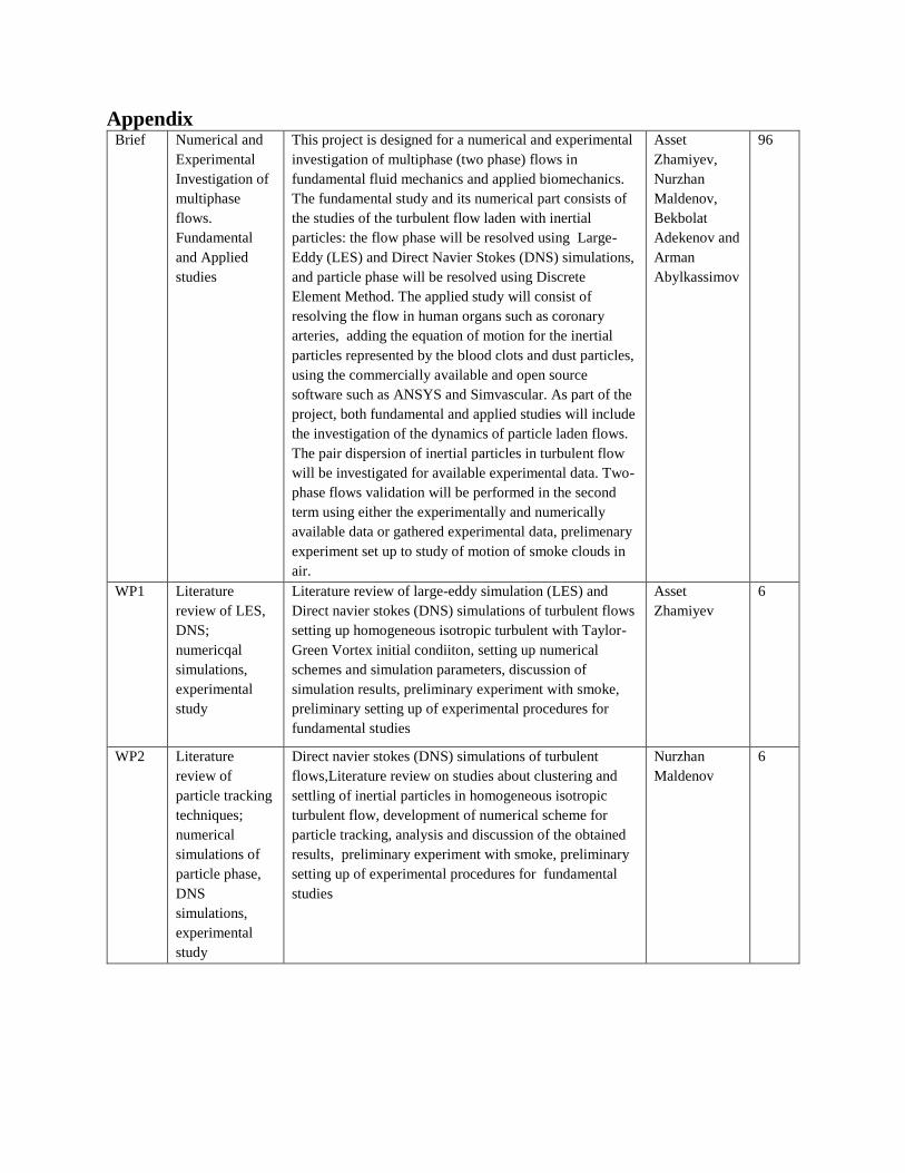
Appendix Brief Numerical and

Experimental

Investigation of

multiphase

flows.

Fundamental

and Applied

studies

This project is designed for a numerical and experimental

investigation of multiphase (two phase) flows in

fundamental fluid mechanics and applied biomechanics.

The fundamental study and its numerical part consists of

the studies of the turbulent flow laden with inertial

particles: the flow phase will be resolved using Large-

Eddy (LES) and Direct Navier Stokes (DNS) simulations,

and particle phase will be resolved using Discrete

Element Method. The applied study will consist of

resolving the flow in human organs such as coronary

arteries, adding the equation of motion for the inertial

particles represented by the blood clots and dust particles,

using the commercially available and open source

software such as ANSYS and Simvascular. As part of the

project, both fundamental and applied studies will include

the investigation of the dynamics of particle laden flows.

The pair dispersion of inertial particles in turbulent flow

will be investigated for available experimental data. Two-

phase flows validation will be performed in the second

term using either the experimentally and numerically

available data or gathered experimental data, prelimenary

experiment set up to study of motion of smoke clouds in

air.

Asset

Zhamiyev,

Nurzhan

Maldenov,

Bekbolat

Adekenov and

Arman

Abylkassimov

96

WP1 Literature

review of LES,

DNS;

numericqal

simulations,

experimental

study

Literature review of large-eddy simulation (LES) and

Direct navier stokes (DNS) simulations of turbulent flows

setting up homogeneous isotropic turbulent with Taylor-

Green Vortex initial condiiton, setting up numerical

schemes and simulation parameters, discussion of

simulation results, preliminary experiment with smoke,

preliminary setting up of experimental procedures for

fundamental studies

Asset

Zhamiyev

6

WP2 Literature

review of

particle tracking

techniques;

numerical

simulations of

particle phase,

DNS

simulations,

experimental

study

Direct navier stokes (DNS) simulations of turbulent

flows,Literature review on studies about clustering and

settling of inertial particles in homogeneous isotropic

turbulent flow, development of numerical scheme for

particle tracking, analysis and discussion of the obtained

results, preliminary experiment with smoke, preliminary

setting up of experimental procedures for fundamental

studies

Nurzhan

Maldenov

6

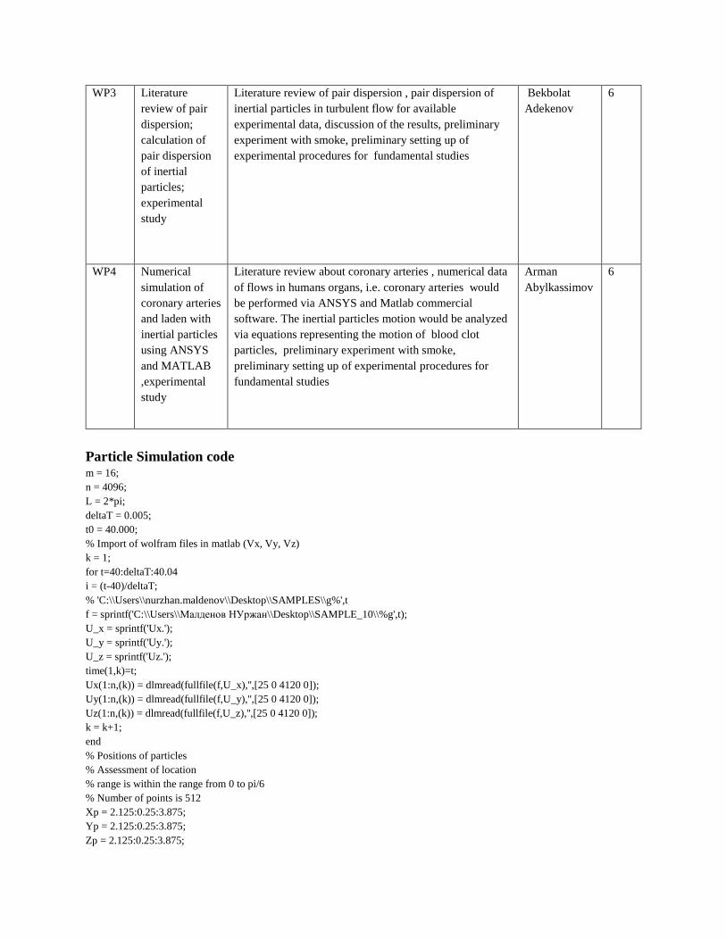
WP3 Literature

review of pair

dispersion;

calculation of

pair dispersion

of inertial

particles;

experimental

study

Literature review of pair dispersion , pair dispersion of

inertial particles in turbulent flow for available

experimental data, discussion of the results, preliminary

experiment with smoke, preliminary setting up of

experimental procedures for fundamental studies

Bekbolat

Adekenov

6

WP4 Numerical

simulation of

coronary arteries

and laden with

inertial particles

using ANSYS

and MATLAB

,experimental

study

Literature review about coronary arteries , numerical data

of flows in humans organs, i.e. coronary arteries would

be performed via ANSYS and Matlab commercial

software. The inertial particles motion would be analyzed

via equations representing the motion of blood clot

particles, preliminary experiment with smoke,

preliminary setting up of experimental procedures for

fundamental studies

Arman

Abylkassimov

6

Particle Simulation code m = 16;

n = 4096;

L = 2*pi;

deltaT = 0.005;

t0 = 40.000;

% Import of wolfram files in matlab (Vx, Vy, Vz)

k = 1;

for t=40:deltaT:40.04

i = (t-40)/deltaT;

% 'C:\\Users\\nurzhan.maldenov\\Desktop\\SAMPLES\\g%',t

f = sprintf('C:\\Users\\Малденов НУржан\\Desktop\\SAMPLE_10\\%g',t);

U_x = sprintf('Ux.');

U_y = sprintf('Uy.');

U_z = sprintf('Uz.');

time(1,k)=t;

Ux(1:n,(k)) = dlmread(fullfile(f,U_x),'',[25 0 4120 0]);

Uy(1:n,(k)) = dlmread(fullfile(f,U_y),'',[25 0 4120 0]);

Uz(1:n,(k)) = dlmread(fullfile(f,U_z),'',[25 0 4120 0]);

k = k+1;

end

% Positions of particles

% Assessment of location

% range is within the range from 0 to pi/6

% Number of points is 512

Xp = 2.125:0.25:3.875;

Yp = 2.125:0.25:3.875;

Zp = 2.125:0.25:3.875;

i = 1;

j = 1;

k = 1;

N = 1;

for i = 1:1:8

x = 2.125+0.25*(i-1);

for j = 1:1:8

y = 2.125+0.25*(j-1);

for k = 1:1:8

z = 2.125+0.25*(k-1);

ZP(:,N) = x;

YP(:,N) = y;

XP(:,N) = z;

Pos(:,N) = [z;y;x];

N = N+1;

end

end

end

Pos(:,:,2) = zeros(3,512);

Pos(:,:,3) = zeros(3,512);

Pos(:,:,4) = zeros(3,512);

Pos(:,:,5) = zeros(3,512);

% Positions corresponding to velocity

for i = 1:1:16

Zf(i) = L/(2*m)+(L/m)*(i-1);

for j = 1:1:16

Yf(j) = L/(2*m)+(L/m)*(j-1);

for k = 1:1:16

Xf(k) = L/(2*m)+(L/m)*(k-1);

Num = k+(j-1)*16+(i-1)*256;

Loc(:,Num) = [Xf(k) Yf(j) Zf(i)];

end

end

end

% Interpolation of Velocity of particles

% Hermite polynomial

[X,Y,Z] = meshgrid(Xf,Yf,Zf)

Xq = XP;

Yq = YP;

Zq = ZP;

% [Xq,Yq,Zq] = meshgrid(Xp,Yp,Zp)

Ux_0 = Ux(:,1);

Uy_0 = Uy(:,1);

Uz_0 = Uz(:,1);

% converting velocity vectors in matrix form

j = 1;

k = 1;

V = zeros(3,512);

V(:,:,2) = zeros(3,512);

V(:,:,3) = zeros(3,512);

N = 1;

for i = 1:1:9

for o = 1:1:4096

k = fix((o-1)/256)+1;

j = fix((o-1-(k-1)*256)/16)+1;

if rem(o,16) == 0

l = 16;

else

l = rem(o,16);

end

U_xf(j,l,k) = Ux(o,i);

U_yf(j,l,k) = Uy(o,i);

U_zf(j,l,k) = Uz(o,i);

gh = 56

end

U_xq = interp3(X,Y,Z,U_xf,Xq,Yq,Zq,'cubic');

U_yq = interp3(X,Y,Z,U_yf,Xq,Yq,Zq,'cubic');

U_zq = interp3(X,Y,Z,U_zf,Xq,Yq,Zq,'cubic');

g_x = zeros(1,512);

g_y = ones(1,512)*(-9.801);

g_z = zeros(1,512);

g = [g_x;g_y;g_z];

U(:,:,i) = [U_xq; U_yq; U_zq]

% Maxey-Riley equation

% Tau_P

Tau_Ita = sqrt(1.7*(10)^(-5)/0.2);

St = 0.1;

Tau_P = St*Tau_Ita;

V(:,:,i+1) = V(:,:,i) - deltaT/Tau_P*(V(:,:,i) - U(:,:,i)) + g*deltaT;

Pos(:,:,i+1) = V(:,:,i)*deltaT + Pos(:,:,i);

Xq = Pos(1,:,i+1)

Yq = Pos(2,:,i+1)

Zq = Pos(3,:,i+1)

% [Xq,Yq,Zq] = meshgrid(Xq1,Yq1,Zq1)

end

% graphs

% Particles(:,:) = Pos(:,:,6);

% Check

Xc = [2.945 2.945 2.9466 2.9415 2.9657 2.8625 3.3167 1.2955 10.2089 -29.2446];

Yc = [2.945 2.945 2.9607 2.907 3.1605 2.0552 6.9599 -14.743 81.2273 -343.3018];

Zc = [2.945 2.945 2.9426 2.9509 2.9118 3.0822 2.3331 5.6469 -9.038 55.89];

%plot3(Pos(1,:,1),Pos(2,:,1),Pos(3,:,1),'.','MarkerSize',50)

% axis([0 2*pi 0 2*pi 0 2*pi])

Pair-dispersion code

Code, which draws the graphs clearvars D2_average D2_normalised D2_raw t T

n=0.431;

tau=0.011;

k=0;

Numel=arrayfun(@(X)(numel(X.dRD2)),meanD2_general);

Max=max(Numel);

for i=1:1:Max

D2_sum=0;

k=k+1;

m=0;

for j=1:1:62

D2_raw=meanD2_general(j+1).dRD2; % Don't Forget to change tau and ita

if numel(D2_raw)>=k

D2=abs(D2_raw(1,k)); %for abs(D2_raw(1,k))

D2_sum=D2_sum+D2;

m=m+1;

end

end

D2_average(i,1)=D2_sum/m;

t(i,1)=1/2600*(i-1);

end

T=t./tau;

D2_normalised=D2_average./n^2;

figure

loglog(T,D2_normalised);

Code, which calculates the average value of results, obtained from 20 different movies.

clearvars D2_average RD2_average R2_average meanD2_general

for e=2:1:63

for i=1:20

string_part =

'D:\Study\Research\Results\MeanD2\meanD2_0p3_0p8_2p5_tracks\meanD2_0p3_0p8_2p5_tracks_';

filename1 = [string_part int2str(i) '_50_100ita.mat'];

load(filename1);

A(i).dRD2=meanD2(e).dRD2;

A(i).dD2=meanD2(e).dD2;

A(i).dR2=meanD2(e).dR2;

end

Numel=arrayfun(@(X)(numel(X.dRD2)),A);

Max=max(Numel);

k=0;

for i=1:1:Max

D2_sum=0;

k=k+1;

m=0;

for j=1:1:20

D2_raw=A(j).dD2;

if numel(D2_raw)>=k

D2=D2_raw(1,k);

D2_sum=D2_sum+D2;

m=m+1;

end

end

D2_average(i,1)=D2_sum/m;

%t(i,1)=1/2600*(i-1);

end

k=0;

for i=1:1:Max

RD2_sum=0;

k=k+1;

m=0;

for j=1:1:20

RD2_raw=A(j).dRD2;

if numel(RD2_raw)>=k

RD2=RD2_raw(1,k);

RD2_sum=RD2_sum+RD2;

m=m+1;

end

end

RD2_average(i,1)=RD2_sum/m;

%t(i,1)=1/2600*(i-1);

end

k=0;

for i=1:1:Max

R2_sum=0;

k=k+1;

m=0;

for j=1:1:20

R2_raw=A(j).dR2;

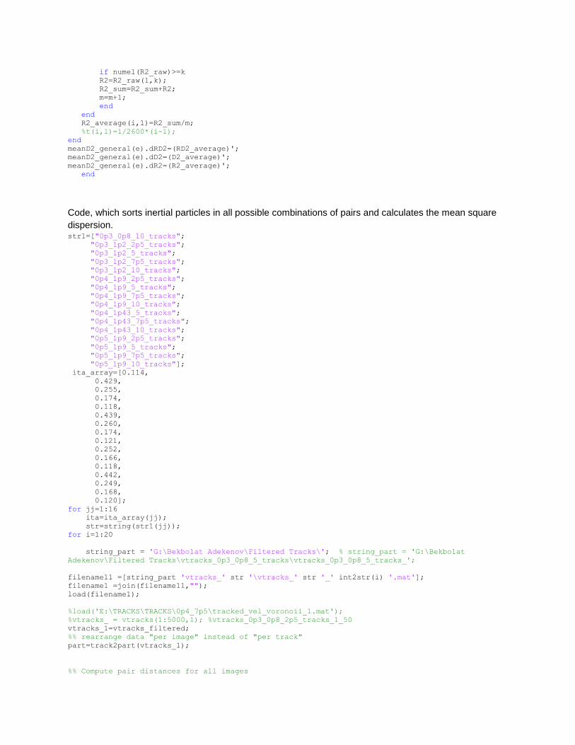
if numel(R2_raw)>=k

R2=R2_raw(1,k);

R2_sum=R2_sum+R2;

m=m+1;

end

end

R2_average(i,1)=R2_sum/m;

%t(i,1)=1/2600*(i-1);

end

meanD2_general(e).dRD2=(RD2_average)';

meanD2_general(e).dD2=(D2_average)';

meanD2_general(e).dR2=(R2_average)';

end

Code, which sorts inertial particles in all possible combinations of pairs and calculates the mean square

dispersion. str1=["0p3_0p8_10_tracks";

"0p3_1p2_2p5_tracks";

"0p3_1p2_5_tracks";

"0p3_1p2_7p5_tracks";

"0p3_1p2_10_tracks";

"0p4_1p9_2p5_tracks";

"0p4_1p9_5_tracks";

"0p4_1p9_7p5_tracks";

"0p4_1p9_10_tracks";

"0p4_1p43_5_tracks";

"0p4_1p43_7p5_tracks";

"0p4_1p43_10_tracks";

"0p5_1p9_2p5_tracks";

"0p5_1p9_5_tracks";

"0p5_1p9_7p5_tracks";

"0p5_1p9_10_tracks"];

ita_array=[0.114,

0.429,

0.255,

0.174,

0.118,

0.439,

0.260,

0.174,

0.121,

0.252,

0.166,

0.118,

0.442,

0.249,

0.168,

0.120];

for jj=1:16

ita=ita_array(jj);

str=string(str1(jj));

for i=1:20

string_part = 'G:\Bekbolat Adekenov\Filtered Tracks\'; % string_part = 'G:\Bekbolat

Adekenov\Filtered Tracks\vtracks_0p3_0p8_5_tracks\vtracks_0p3_0p8_5_tracks_';

filename11 =[string_part 'vtracks_' str '\vtracks_' str '_' int2str(i) '.mat'];

filename1 =join(filename11,"");

load(filename1);

%load('E:\TRACKS\TRACKS\0p4_7p5\tracked_vel_voronoii_1.mat');

%vtracks_ = vtracks(1:5000,1); %vtracks_0p3_0p8_2p5_tracks_1_50

vtracks_1=vtracks_filtered;

%% rearrange data "per image" instead of "per track"

part=track2part(vtracks_1);

%% Compute pair distances for all images

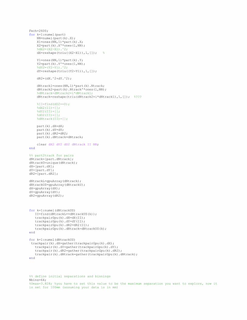
Fech=2600;

for k=1:numel(part)

NN=numel(part(k).X);

X1=ones(NN,1)*part(k).X;

X2=part(k).X'*ones(1,NN);

%dX2=(X2-X1).^2;

dX=reshape(triu((X2-X1)),1,[]); %

Y1=ones(NN,1)*part(k).Y;

Y2=part(k).Y'*ones(1,NN);

%dY2=(Y2-Y1).^2;

dY=reshape(triu((Y2-Y1)),1,[]);

dR2=(dX.^2+dY.^2);

dNtrack1=ones(NN,1)*part(k).Ntrack;

dNtrack2=part(k).Ntrack'*ones(1,NN);

%dNtrack=dNtrack2+i*dNtrack1;

dNtrack=reshape(triu(dNtrack2+i*dNtrack1),1,[]); %???

%II=find(dD2==0);

%dX2(II)=[];

%dY2(II)=[];

%dD2(II)=[];

%dNtrack(II)=[];

part(k).dX=dX;

part(k).dY=dY;

part(k).dR2=dR2;

part(k).dNtrack=dNtrack;

clear dX2 dY2 dD2 dNtrack II NN;

end

%% part2track for pairs

dNtrack=[part.dNtrack];

dNtrackU=unique(dNtrack);

dX=[part.dX];

dY=[part.dY];

dR2=[part.dR2];

dNtrackL=gpuArray(dNtrack);

dNtrackUS=gpuArray(dNtrackU);

dX=gpuArray(dX);

dY=gpuArray(dY);

dR2=gpuArray(dR2);

for k=1:numel(dNtrackUS)

II=find(dNtrackL==dNtrackUS(k));

trackpairGpu(k).dX=dX(II);

trackpairGpu(k).dY=dY(II);

trackpairGpu(k).dR2=dR2(II);

trackpairGpu(k).dNtrack=dNtrackUS(k);

end

for k=1:numel(dNtrackUS)

trackpair(k).dX=gather(trackpairGpu(k).dX);

trackpair(k).dY=gather(trackpairGpu(k).dY);

trackpair(k).dR2=gather(trackpairGpu(k).dR2);

trackpair(k).dNtrack=gather(trackpairGpu(k).dNtrack);

end

%% define initial separations and binnings

Nbins=64;

%Dmax=3.828; %you have to set this value to be the maximum separation you want to explore, now it

is set for 100mm (assuming your data is in mm)

Dmax=100*ita;

dX0=arrayfun(@(X)(abs(X.dX(1))),trackpair);

dY0=arrayfun(@(X)(abs(X.dY(1))),trackpair);

dR20=arrayfun(@(X)(X.dR2(1)),trackpair);

edgesX=linspace(0,Dmax,Nbins);

edgesY=linspace(0,Dmax,Nbins);

edgesR2=linspace(0,Dmax^2,Nbins);

binX=(edgesX(2:end)+edgesX(1:end-1))/2;

binY=(edgesY(2:end)+edgesY(1:end-1))/2;

binR2=(edgesR2(2:end)+edgesR2(1:end-1))/2;

%%

[NX,binX0]=histc(dX0,edgesX);

[NY,binY0]=histc(dY0,edgesY);

[NR2,binR20]=histc(dR20,edgesR2);

for k=2:numel(binX)

% IX=find(binX0==k);

% IY=find(binY0==k);

IR=find(binR20==k);

% for statistics on 1D separation, we still condition on the 2D separation

% R20 to avoid combining for instance particles with small separation in X but actually very much

separated in Y

IX=IR;

IY=IR;

dX2=arrayfun(@(X)((X.dX-X.dX(1)).^2),trackpair(IX),'UniformOutput',false);

dY2=arrayfun(@(X)((X.dY-X.dY(1)).^2),trackpair(IY),'UniformOutput',false);

dR2=arrayfun(@(X)(X.dR2-X.dR2(1)),trackpair(IR),'UniformOutput',false);

dD2=arrayfun(@(X)((X.dX-X.dX(1)).^2+(X.dY-X.dY(1)).^2),trackpair(IR),'UniformOutput',false);

dRD2=arrayfun(@(X)(X.dR2),trackpair(IR),'UniformOutput',false);

NX=cellfun(@(X)(numel(X)),dX2);

NY=cellfun(@(X)(numel(X)),dY2);

NR=cellfun(@(X)(numel(X)),dR2);

ND=cellfun(@(X)(numel(X)),dD2);

NRD=cellfun(@(X)(numel(X)),dRD2);

MX2=NaN(numel(dX2),max(NX));

MY2=NaN(numel(dY2),max(NY));

MR2=NaN(numel(dD2),max(NR));

MD2=NaN(numel(dD2),max(ND));

MRD2=NaN(numel(dRD2),max(NRD));

for kk=1:numel(dX2)

MX2(kk,1:NX(kk))=dX2{kk};

end

for kk=1:numel(dY2)

MY2(kk,1:NY(kk))=dY2{kk};

end

for kk=1:numel(dR2)

MR2(kk,1:NR(kk))=dR2{kk};

end

for kk=1:numel(dD2)

MD2(kk,1:ND(kk))=dD2{kk};

end

for kk=1:numel(dRD2)

MRD2(kk,1:NRD(kk))=dRD2{kk};

end

dX2=nanmean(MX2,1);

dY2=nanmean(MY2,1);

dR2=nanmean(MY2,1);

dD2=nanmean(MD2,1);

dRD2=nanmean(MRD2,1);

dX2(dX2==NaN)=[];

dY2(dY2==NaN)=[];

dR2(dR2==NaN)=[];

dD2(dD2==NaN)=[];

dRD2(dRD2==NaN)=[];

meanD2(k).dX2=nanmean(MX2,1);

meanD2(k).dY2=nanmean(MY2,1);

meanD2(k).dR2=nanmean(MR2,1);

meanD2(k).dD2=nanmean(MD2,1);

meanD2(k).dRD2=nanmean(MRD2,1);

meanD2(k).TX=[0:numel(dX2)-1]/Fech;% you need to define Fech (sampling frequencey) in the

workspace

meanD2(k).TY=[0:numel(dY2)-1]/Fech;% you need to define Fech (sampling frequencey) in the

workspace

meanD2(k).TR=[0:numel(dR2)-1]/Fech;% you need to define Fech (sampling frequencey) in the

workspace

meanD2(k).TD=[0:numel(dD2)-1]/Fech;% you need to define Fech (sampling frequencey) in the

workspace

meanD2(k).dX20=mean(arrayfun(@(X)(X.dX(1).^2),trackpair(IR)));

meanD2(k).dY20=mean(arrayfun(@(X)(X.dY(1).^2),trackpair(IR)));

meanD2(k).dR20=binR2(k);

clear MX2;

end

string_part_2 = 'G:\Bekbolat Adekenov\Results\results_'; %string_part_2 = 'G:\Bekbolat

Adekenov\Results\results_0p3_0p8_5_tracks\meanD2_0p3_0p8_5_tracks\meanD2_0p3_0p8_5_tracks_';

filename22 = [string_part_2 str '\meanD2_' str '\meanD2_' str '_' int2str(i) '_100ita.mat'];

filename2 =join(filename22,"");

save(filename2,'meanD2')

string_part_3 = 'G:\Bekbolat Adekenov\Results\results_'; %string_part_3 = 'G:\Bekbolat

Adekenov\Results\results_0p3_0p8_5_tracks\trackpair_0p3_0p8_5_tracks\trackpair_0p3_0p8_5_tracks_'

;

filename33 = [string_part_3 str '\trackpair_' str '\trackpair_' str '_' int2str(i) '.mat'];

filename3 =join(filename33,"");

save(filename3,'trackpair')

clearvars MX2 MY2 MR2 MD2 MRD2

Nbins=64;

%Dmax=3.828; %you have to set this value to be the maximum separation you want to explore, now it

is set for 100mm (assuming your data is in mm)

Dmax=60*ita;

dX0=arrayfun(@(X)(abs(X.dX(1))),trackpair);

dY0=arrayfun(@(X)(abs(X.dY(1))),trackpair);

dR20=arrayfun(@(X)(X.dR2(1)),trackpair);

edgesX=linspace(0,Dmax,Nbins);

edgesY=linspace(0,Dmax,Nbins);

edgesR2=linspace(0,Dmax^2,Nbins);

binX=(edgesX(2:end)+edgesX(1:end-1))/2;

binY=(edgesY(2:end)+edgesY(1:end-1))/2;

binR2=(edgesR2(2:end)+edgesR2(1:end-1))/2;

%%

[NX,binX0]=histc(dX0,edgesX);

[NY,binY0]=histc(dY0,edgesY);

[NR2,binR20]=histc(dR20,edgesR2);

for k=2:numel(binX)

% IX=find(binX0==k);

% IY=find(binY0==k);

IR=find(binR20==k);

% for statistics on 1D separation, we still condition on the 2D separation

% R20 to avoid combining for instance particles with small separation in X but actually very much

separated in Y

IX=IR;

IY=IR;

dX2=arrayfun(@(X)((X.dX-X.dX(1)).^2),trackpair(IX),'UniformOutput',false);

dY2=arrayfun(@(X)((X.dY-X.dY(1)).^2),trackpair(IY),'UniformOutput',false);

dR2=arrayfun(@(X)(X.dR2-X.dR2(1)),trackpair(IR),'UniformOutput',false);

dD2=arrayfun(@(X)((X.dX-X.dX(1)).^2+(X.dY-X.dY(1)).^2),trackpair(IR),'UniformOutput',false);

dRD2=arrayfun(@(X)(X.dR2),trackpair(IR),'UniformOutput',false);

NX=cellfun(@(X)(numel(X)),dX2);

NY=cellfun(@(X)(numel(X)),dY2);

NR=cellfun(@(X)(numel(X)),dR2);

ND=cellfun(@(X)(numel(X)),dD2);

NRD=cellfun(@(X)(numel(X)),dRD2);

MX2=NaN(numel(dX2),max(NX));

MY2=NaN(numel(dY2),max(NY));

MR2=NaN(numel(dD2),max(NR));

MD2=NaN(numel(dD2),max(ND));

MRD2=NaN(numel(dRD2),max(NRD));

for kk=1:numel(dX2)

MX2(kk,1:NX(kk))=dX2{kk};

end

for kk=1:numel(dY2)

MY2(kk,1:NY(kk))=dY2{kk};

end

for kk=1:numel(dR2)

MR2(kk,1:NR(kk))=dR2{kk};

end

for kk=1:numel(dD2)

MD2(kk,1:ND(kk))=dD2{kk};

end

for kk=1:numel(dRD2)

MRD2(kk,1:NRD(kk))=dRD2{kk};

end

dX2=nanmean(MX2,1);

dY2=nanmean(MY2,1);

dR2=nanmean(MY2,1);

dD2=nanmean(MD2,1);

dRD2=nanmean(MRD2,1);

dX2(dX2==NaN)=[];

dY2(dY2==NaN)=[];

dR2(dR2==NaN)=[];

dD2(dD2==NaN)=[];

dRD2(dRD2==NaN)=[];

meanD2(k).dX2=nanmean(MX2,1);

meanD2(k).dY2=nanmean(MY2,1);

meanD2(k).dR2=nanmean(MR2,1);

meanD2(k).dD2=nanmean(MD2,1);

meanD2(k).dRD2=nanmean(MRD2,1);

meanD2(k).TX=[0:numel(dX2)-1]/Fech;% you need to define Fech (sampling frequencey) in the

workspace

meanD2(k).TY=[0:numel(dY2)-1]/Fech;% you need to define Fech (sampling frequencey) in the

workspace

meanD2(k).TR=[0:numel(dR2)-1]/Fech;% you need to define Fech (sampling frequencey) in the

workspace

meanD2(k).TD=[0:numel(dD2)-1]/Fech;% you need to define Fech (sampling frequencey) in the

workspace

meanD2(k).dX20=mean(arrayfun(@(X)(X.dX(1).^2),trackpair(IR)));

meanD2(k).dY20=mean(arrayfun(@(X)(X.dY(1).^2),trackpair(IR)));

meanD2(k).dR20=binR2(k);

clear MX2;

end

filename22 = [string_part_2 str '\meanD2_' str '\meanD2_' str '_' int2str(i) '_60ita.mat'];

filename2 =join(filename22,"");

save(filename2,'meanD2')

clearvars MX2 MY2 MR2 MD2 MRD2

Nbins=64;

%Dmax=3.828; %you have to set this value to be the maximum separation you want to explore, now it

is set for 100mm (assuming your data is in mm)

Dmax=36*ita;

dX0=arrayfun(@(X)(abs(X.dX(1))),trackpair);

dY0=arrayfun(@(X)(abs(X.dY(1))),trackpair);

dR20=arrayfun(@(X)(X.dR2(1)),trackpair);

edgesX=linspace(0,Dmax,Nbins);

edgesY=linspace(0,Dmax,Nbins);

edgesR2=linspace(0,Dmax^2,Nbins);

binX=(edgesX(2:end)+edgesX(1:end-1))/2;

binY=(edgesY(2:end)+edgesY(1:end-1))/2;

binR2=(edgesR2(2:end)+edgesR2(1:end-1))/2;

%%

[NX,binX0]=histc(dX0,edgesX);

[NY,binY0]=histc(dY0,edgesY);

[NR2,binR20]=histc(dR20,edgesR2);

for k=2:numel(binX)

% IX=find(binX0==k);

% IY=find(binY0==k);

IR=find(binR20==k);

% for statistics on 1D separation, we still condition on the 2D separation

% R20 to avoid combining for instance particles with small separation in X but actually very much

separated in Y

IX=IR;

IY=IR;

dX2=arrayfun(@(X)((X.dX-X.dX(1)).^2),trackpair(IX),'UniformOutput',false);

dY2=arrayfun(@(X)((X.dY-X.dY(1)).^2),trackpair(IY),'UniformOutput',false);

dR2=arrayfun(@(X)(X.dR2-X.dR2(1)),trackpair(IR),'UniformOutput',false);

dD2=arrayfun(@(X)((X.dX-X.dX(1)).^2+(X.dY-X.dY(1)).^2),trackpair(IR),'UniformOutput',false);

dRD2=arrayfun(@(X)(X.dR2),trackpair(IR),'UniformOutput',false);

NX=cellfun(@(X)(numel(X)),dX2);

NY=cellfun(@(X)(numel(X)),dY2);

NR=cellfun(@(X)(numel(X)),dR2);

ND=cellfun(@(X)(numel(X)),dD2);

NRD=cellfun(@(X)(numel(X)),dRD2);

MX2=NaN(numel(dX2),max(NX));

MY2=NaN(numel(dY2),max(NY));

MR2=NaN(numel(dD2),max(NR));

MD2=NaN(numel(dD2),max(ND));

MRD2=NaN(numel(dRD2),max(NRD));

for kk=1:numel(dX2)

MX2(kk,1:NX(kk))=dX2{kk};

end

for kk=1:numel(dY2)

MY2(kk,1:NY(kk))=dY2{kk};

end

for kk=1:numel(dR2)

MR2(kk,1:NR(kk))=dR2{kk};

end

for kk=1:numel(dD2)

MD2(kk,1:ND(kk))=dD2{kk};

end

for kk=1:numel(dRD2)

MRD2(kk,1:NRD(kk))=dRD2{kk};

end

dX2=nanmean(MX2,1);

dY2=nanmean(MY2,1);

dR2=nanmean(MY2,1);

dD2=nanmean(MD2,1);

dRD2=nanmean(MRD2,1);

dX2(dX2==NaN)=[];

dY2(dY2==NaN)=[];

dR2(dR2==NaN)=[];

dD2(dD2==NaN)=[];

dRD2(dRD2==NaN)=[];

meanD2(k).dX2=nanmean(MX2,1);

meanD2(k).dY2=nanmean(MY2,1);

meanD2(k).dR2=nanmean(MR2,1);

meanD2(k).dD2=nanmean(MD2,1);

meanD2(k).dRD2=nanmean(MRD2,1);

meanD2(k).TX=[0:numel(dX2)-1]/Fech;% you need to define Fech (sampling frequencey) in the

workspace

meanD2(k).TY=[0:numel(dY2)-1]/Fech;% you need to define Fech (sampling frequencey) in the

workspace

meanD2(k).TR=[0:numel(dR2)-1]/Fech;% you need to define Fech (sampling frequencey) in the

workspace

meanD2(k).TD=[0:numel(dD2)-1]/Fech;% you need to define Fech (sampling frequencey) in the

workspace

meanD2(k).dX20=mean(arrayfun(@(X)(X.dX(1).^2),trackpair(IR)));

meanD2(k).dY20=mean(arrayfun(@(X)(X.dY(1).^2),trackpair(IR)));

meanD2(k).dR20=binR2(k);

clear MX2;

end

filename22 = [string_part_2 str '\meanD2_' str '\meanD2_' str '_' int2str(i) '_36ita.mat'];

filename2 =join(filename22,"");

save(filename2,'meanD2')

clearvars MX2 MY2 MR2 MD2 MRD2

Nbins=64;

%Dmax=3.828; %you have to set this value to be the maximum separation you want to explore, now it

is set for 100mm (assuming your data is in mm)

Dmax=22*ita;

dX0=arrayfun(@(X)(abs(X.dX(1))),trackpair);

dY0=arrayfun(@(X)(abs(X.dY(1))),trackpair);

dR20=arrayfun(@(X)(X.dR2(1)),trackpair);

edgesX=linspace(0,Dmax,Nbins);

edgesY=linspace(0,Dmax,Nbins);

edgesR2=linspace(0,Dmax^2,Nbins);

binX=(edgesX(2:end)+edgesX(1:end-1))/2;

binY=(edgesY(2:end)+edgesY(1:end-1))/2;

binR2=(edgesR2(2:end)+edgesR2(1:end-1))/2;

%%

[NX,binX0]=histc(dX0,edgesX);

[NY,binY0]=histc(dY0,edgesY);

[NR2,binR20]=histc(dR20,edgesR2);

for k=2:numel(binX)

% IX=find(binX0==k);

% IY=find(binY0==k);

IR=find(binR20==k);

% for statistics on 1D separation, we still condition on the 2D separation

% R20 to avoid combining for instance particles with small separation in X but actually very much

separated in Y

IX=IR;

IY=IR;

dX2=arrayfun(@(X)((X.dX-X.dX(1)).^2),trackpair(IX),'UniformOutput',false);

dY2=arrayfun(@(X)((X.dY-X.dY(1)).^2),trackpair(IY),'UniformOutput',false);

dR2=arrayfun(@(X)(X.dR2-X.dR2(1)),trackpair(IR),'UniformOutput',false);

dD2=arrayfun(@(X)((X.dX-X.dX(1)).^2+(X.dY-X.dY(1)).^2),trackpair(IR),'UniformOutput',false);

dRD2=arrayfun(@(X)(X.dR2),trackpair(IR),'UniformOutput',false);

NX=cellfun(@(X)(numel(X)),dX2);

NY=cellfun(@(X)(numel(X)),dY2);

NR=cellfun(@(X)(numel(X)),dR2);

ND=cellfun(@(X)(numel(X)),dD2);

NRD=cellfun(@(X)(numel(X)),dRD2);

MX2=NaN(numel(dX2),max(NX));

MY2=NaN(numel(dY2),max(NY));

MR2=NaN(numel(dD2),max(NR));

MD2=NaN(numel(dD2),max(ND));

MRD2=NaN(numel(dRD2),max(NRD));

for kk=1:numel(dX2)

MX2(kk,1:NX(kk))=dX2{kk};

end

for kk=1:numel(dY2)

MY2(kk,1:NY(kk))=dY2{kk};

end

for kk=1:numel(dR2)

MR2(kk,1:NR(kk))=dR2{kk};

end

for kk=1:numel(dD2)

MD2(kk,1:ND(kk))=dD2{kk};

end

for kk=1:numel(dRD2)

MRD2(kk,1:NRD(kk))=dRD2{kk};

end

dX2=nanmean(MX2,1);

dY2=nanmean(MY2,1);

dR2=nanmean(MY2,1);

dD2=nanmean(MD2,1);

dRD2=nanmean(MRD2,1);

dX2(dX2==NaN)=[];

dY2(dY2==NaN)=[];

dR2(dR2==NaN)=[];

dD2(dD2==NaN)=[];

dRD2(dRD2==NaN)=[];

meanD2(k).dX2=nanmean(MX2,1);

meanD2(k).dY2=nanmean(MY2,1);

meanD2(k).dR2=nanmean(MR2,1);

meanD2(k).dD2=nanmean(MD2,1);

meanD2(k).dRD2=nanmean(MRD2,1);

meanD2(k).TX=[0:numel(dX2)-1]/Fech;% you need to define Fech (sampling frequencey) in the

workspace

meanD2(k).TY=[0:numel(dY2)-1]/Fech;% you need to define Fech (sampling frequencey) in the

workspace

meanD2(k).TR=[0:numel(dR2)-1]/Fech;% you need to define Fech (sampling frequencey) in the

workspace

meanD2(k).TD=[0:numel(dD2)-1]/Fech;% you need to define Fech (sampling frequencey) in the

workspace

meanD2(k).dX20=mean(arrayfun(@(X)(X.dX(1).^2),trackpair(IR)));

meanD2(k).dY20=mean(arrayfun(@(X)(X.dY(1).^2),trackpair(IR)));

meanD2(k).dR20=binR2(k);

clear MX2;

end

filename22 = [string_part_2 str '\meanD2_' str '\meanD2_' str '_' int2str(i) '_22ita.mat'];

filename2 =join(filename22,"");

save(filename2,'meanD2')

clearvars MX2 MY2 MR2 MD2 MRD2

Nbins=64;

%Dmax=3.828; %you have to set this value to be the maximum separation you want to explore, now it

is set for 100mm (assuming your data is in mm)

Dmax=13*ita;

dX0=arrayfun(@(X)(abs(X.dX(1))),trackpair);

dY0=arrayfun(@(X)(abs(X.dY(1))),trackpair);

dR20=arrayfun(@(X)(X.dR2(1)),trackpair);

edgesX=linspace(0,Dmax,Nbins);

edgesY=linspace(0,Dmax,Nbins);

edgesR2=linspace(0,Dmax^2,Nbins);

binX=(edgesX(2:end)+edgesX(1:end-1))/2;

binY=(edgesY(2:end)+edgesY(1:end-1))/2;

binR2=(edgesR2(2:end)+edgesR2(1:end-1))/2;

%%

[NX,binX0]=histc(dX0,edgesX);

[NY,binY0]=histc(dY0,edgesY);

[NR2,binR20]=histc(dR20,edgesR2);

for k=2:numel(binX)

% IX=find(binX0==k);

% IY=find(binY0==k);

IR=find(binR20==k);

% for statistics on 1D separation, we still condition on the 2D separation

% R20 to avoid combining for instance particles with small separation in X but actually very much

separated in Y

IX=IR;

IY=IR;

dX2=arrayfun(@(X)((X.dX-X.dX(1)).^2),trackpair(IX),'UniformOutput',false);

dY2=arrayfun(@(X)((X.dY-X.dY(1)).^2),trackpair(IY),'UniformOutput',false);

dR2=arrayfun(@(X)(X.dR2-X.dR2(1)),trackpair(IR),'UniformOutput',false);

dD2=arrayfun(@(X)((X.dX-X.dX(1)).^2+(X.dY-X.dY(1)).^2),trackpair(IR),'UniformOutput',false);

dRD2=arrayfun(@(X)(X.dR2),trackpair(IR),'UniformOutput',false);

NX=cellfun(@(X)(numel(X)),dX2);

NY=cellfun(@(X)(numel(X)),dY2);

NR=cellfun(@(X)(numel(X)),dR2);

ND=cellfun(@(X)(numel(X)),dD2);

NRD=cellfun(@(X)(numel(X)),dRD2);

MX2=NaN(numel(dX2),max(NX));

MY2=NaN(numel(dY2),max(NY));

MR2=NaN(numel(dD2),max(NR));

MD2=NaN(numel(dD2),max(ND));

MRD2=NaN(numel(dRD2),max(NRD));

for kk=1:numel(dX2)

MX2(kk,1:NX(kk))=dX2{kk};

end

for kk=1:numel(dY2)

MY2(kk,1:NY(kk))=dY2{kk};

end

for kk=1:numel(dR2)

MR2(kk,1:NR(kk))=dR2{kk};

end

for kk=1:numel(dD2)

MD2(kk,1:ND(kk))=dD2{kk};

end

for kk=1:numel(dRD2)

MRD2(kk,1:NRD(kk))=dRD2{kk};

end

dX2=nanmean(MX2,1);

dY2=nanmean(MY2,1);

dR2=nanmean(MY2,1);

dD2=nanmean(MD2,1);

dRD2=nanmean(MRD2,1);

dX2(dX2==NaN)=[];

dY2(dY2==NaN)=[];

dR2(dR2==NaN)=[];

dD2(dD2==NaN)=[];

dRD2(dRD2==NaN)=[];

meanD2(k).dX2=nanmean(MX2,1);

meanD2(k).dY2=nanmean(MY2,1);

meanD2(k).dR2=nanmean(MR2,1);

meanD2(k).dD2=nanmean(MD2,1);

meanD2(k).dRD2=nanmean(MRD2,1);

meanD2(k).TX=[0:numel(dX2)-1]/Fech;% you need to define Fech (sampling frequencey) in the

workspace

meanD2(k).TY=[0:numel(dY2)-1]/Fech;% you need to define Fech (sampling frequencey) in the

workspace

meanD2(k).TR=[0:numel(dR2)-1]/Fech;% you need to define Fech (sampling frequencey) in the

workspace

meanD2(k).TD=[0:numel(dD2)-1]/Fech;% you need to define Fech (sampling frequencey) in the

workspace

meanD2(k).dX20=mean(arrayfun(@(X)(X.dX(1).^2),trackpair(IR)));

meanD2(k).dY20=mean(arrayfun(@(X)(X.dY(1).^2),trackpair(IR)));

meanD2(k).dR20=binR2(k);

clear MX2;

end

filename22 = [string_part_2 str '\meanD2_' str '\meanD2_' str '_' int2str(i) '_13ita.mat'];

filename2 =join(filename22,"");

save(filename2,'meanD2')

clearvars trackpair MX2 MY2 MR2 MD2 MRD2

end

end