Numerical Analysis of the Relation between Interactions ...

Numerical Analysis of the Relation

between Interactions and Structure

in a Molecular Fluid

Dissertationzur Erlangung des Grades

“Doktor der Naturwissenschaften”am Fachbereich Physik, Mathematik und Informatik

der Johannes Gutenberg-Universität

in Mainz

Dmitry Ivanizkigeb. in Winsili (Russland)

Mainz 2015

1. Berichterstatter:2. Berichterstatter:

Datum der mündlichen Prüfung: 11. Dezember 2015

D77 - Mainzer Dissertation

Abstract

Coarse graining is a popular technique used in physics to speed up the computer simula-tion of molecular fluids. An essential part of this technique is a method that solves theinverse problem of determining the interaction potential or its parameters from the givenstructural data [PK-2010]. Due to discrepancies between model and reality, the potentialis not unique, such that stability of such method and its convergence to a meaningfulsolution are issues.

In this work, we investigate empirically whether coarse graining can be improved byapplying the theory of inverse problems from applied mathematics. In particular, weuse the singular value analysis to reveal the weak interaction parameters, that have anegligible influence on the structure of the fluid and which cause non-uniqueness of thesolution. Further, we apply a regularizing Levenberg-Marquardt method, which is stableagainst the mentioned discrepancies [Hanke-1997]. Then, we compare it to the existingphysical methods – the Iterative Boltzmann Inversion [Soper-1996] and the Inverse MonteCarlo method [LL-1995], which are fast and well adapted to the problem, but sometimeshave convergence problems [RJLKA-2009], [MFKV-2007].

From analysis of the Iterative Boltzmann Inversion, we elaborate a meaningful appro-ximation of the structure and use it to derive a modification of the Levenberg-Marquardtmethod. We engage the latter for reconstruction of the interaction parameters fromexperimental data for liquid argon and nitrogen. We show that the modified method isstable, convergent and fast. Further, the singular value analysis of the structure and itsapproximation allows to determine the crucial interaction parameters, that is, to simplifythe modeling of interactions. Therefore, our results build a rigorous bridge between theinverse problem from physics and the powerful solution tools from mathematics.

i

Acknowledgment

In the first place, I want to thank my advisors for the highly interesting topic and theguidance during all these years of work.

Further, I thank the numerical and functional analysis groups for a friendly environ-ment in both cooperative and social aspects. I am also very grateful to my colleagues formany fruitful discussions and for improving my english writing skills.

Finally, I acknowledge the “Computational Science Mainz” for funding the first yearof my promotion and offering the opportunity to meet other PhD-students in variousinterdisciplinary workshops. I also want to give a credit to The Mathworks, Inc., whoseproduct MATLAB R© was used for implementation of the algorithms and for creation ofall pictures in this work.

iii

Preface

For the beginning, we want to highlight the interdisciplinary character of this work moti-vated by coarse graining. Two completely different sciences, the statistical physics and theapplied mathematics, contribute equally to the topic. While the motivation of the topiclies in the advanced levels of modern physics, we treat the problem arising there from aviewpoint of equally modern mathematical theory. Even if we can apply the mathema-tical solution methods without studying the entire physical background of the problem,we need a basic physical understanding for interpretation of the results. Since each ofthe two sciences requires an appropriate introduction, we shield in Chapter 1 only theterms, which are necessary for weaving the sciences together. We sketch many ambientconcepts, like interactions and structure, just to return to them later in the work, whenwe elaborate more rigorous definitions. Amongst other things, we introduce the inverseproblem of determining the interaction potential from the structural data given by theradial distribution function (RDF).

In Chapter 2, we explain the mathematical concept of an ill-posed inverse problem anddiscuss the solution theory. We stress that an ill-posed problem describes a model withinstable relation between input and output, such that a regularization is required. Weshow how the singular value decomposition can be used to reveal the instabilities of themodel. Finally, we present the regularizing Levenberg-Marquardt method (LM), solvingsuch problems iteratively, and a condition for its convergence.

We start Chapter 3 with a rigorous derivation of the functional spaces for potentialsand RDFs, in order to apply the theory to the particular inverse problem. We motivatewhy the problem is ill-posed and adapt the LM to the previously derived spaces. We alsokeep in mind the physical background of the problem by discussing the direct problem,where the RDF is computed from the given potential by molecular simulation. We testthe LM in a well-posed, two-dimensional setting and then successfully apply the methodon realistic problems where the experimentally measured RDFs are given as data.

In order to improve our method, we turn in Chapter 4 to the existing, physically moti-vated methods, the Iterative Boltzmann Inversion and the Inverse Monte Carlo method.We show that the reason for their success is a clever approximation of the RDF, andmodify the LM in a similar way. Then, we prove the convergence condition for the LMin the framework of this approximation and apply the modified method to the realisticinverse problems we studied earlier. Further, we discuss a suitable approximation of theunderlying potential and its parameters. We conclude the work by illustrating our resultsin Chapter 5.

We supply this work with two appendices. Appendix A introduces the basics of sta-tistical physics needed for understanding the concept of the RDF. We follow the classicalterminology and do not pretend to cover a complete state of art, but we define a simplerigorous framework sufficient for showing some useful theorems. Appendix B focuses ofthe crucial points of molecular simulation, which play an important role in our discussion.

v

A Word about Notation

In fact, notation deserves a separate section in this work, because every science has itsown preferences about notations, and conflicts cannot be avoided where two sciences cometogether. For instance, σ is a parameter in physics, a singular value in analysis and astandard deviation in statistics. Therefore, we make many subjective conventions andshield them here.

We denote with d the dimension of the Euclidean space, that is, for the most part, itequals three, with exception of some theoretical considerations, where the dimension canbe general, and some illustrative special cases, where the lower dimensions become interes-ting. Throughout the work, the letterD denotes the derivative operator and 1 the identityoperator, where the relevant variables and their number are clear from the context. Wealso use the notation of the gradient operator ~∇, if the derivative is taken in Rd. Further,we write ∂

∂vfor the partial derivative with respect to variable v, such that lower indices

never mean derivatives and always mean indices, components and labels. We supplythe vectors from Rd with arrows, and, in order to distinguish between vector’s index andcomponent, we put the index in parentheses above the vector, for instance, ~e(i)|1 ≤ i ≤ dis the standard base of the Euclidean space. B(r) denotes the open ball of the radius raround origin in Rd. ∂Ω designates the boundary of a domain Ω, that is, ∂B(r) is thesphere of the radius r around origin. We want to be able to distinguish between the samevariable/space/map in the continuous and the discrete formulations, x,X, F and x,X,F,respectively. However, since the discretization is always straight-forward, one can alsoignore the differences of the formulations and typefonts, if not specified otherwise. For afunction f of variables s1, . . . , sJ and parameters x1, . . . , xI , we write

f(s1, . . . , sJ ; x1, . . . , xI)

orf [x1, . . . , xI ](s1, . . . , sJ)

and omit some of the letters, if they do not matter in the current consideration. Further,we label the analytical theorems with A1, A2, etc. and the physical theorems with P1,P2, etc. Both kinds are proven, but the mathematical ones are bound to our model, whilethe physical theorems refer to different models used in physics simultaneously.

Due to an immense number of variables in the appendices devoted to statistical physics,we deviate from the above notations in the following cases. Since the components ofvectors are never mentioned, we put the vector indices below the vectors. For vectorfamilies ~Xi1≤i≤N ⊂ Rd, we consequently use the notations

X :=

~X1

. . .~XN

,

~Xij := ~Xi − ~Xj.

vii

We omit multiple integrals and integrate over the usual domain, if not specified otherwise.In other words, for variables ~X, ~Y ∈ Ω ⊆ Rd, we define

∫

. . . d ~Xd~Y :=

∫

Ω

∫

Ω

. . . d ~Xd~Y .

For an even better readability, we supply this work with lists of all symbols (see p. 149)and abbreviations (see p. 153), as well as with an index where every namebearing conceptappears.

viii

Contents

1 Introduction 11.1 Coarse Graining . . . . . . . . . . . . . . . . . . . . . . . . . . . . . . . . . 11.2 Interactions and Structure . . . . . . . . . . . . . . . . . . . . . . . . . . . 31.3 Subtleties of the Coarse Graining . . . . . . . . . . . . . . . . . . . . . . . 7

2 Theory of Inverse Problems 132.1 Ill-posed Problems . . . . . . . . . . . . . . . . . . . . . . . . . . . . . . . 132.2 Moore-Penrose Inverse . . . . . . . . . . . . . . . . . . . . . . . . . . . . . 142.3 Regularization . . . . . . . . . . . . . . . . . . . . . . . . . . . . . . . . . . 202.4 Tikhonov Regularization . . . . . . . . . . . . . . . . . . . . . . . . . . . . 232.5 Parameter Choice Strategies . . . . . . . . . . . . . . . . . . . . . . . . . . 252.6 Nonlinear Problems . . . . . . . . . . . . . . . . . . . . . . . . . . . . . . . 292.7 Summary . . . . . . . . . . . . . . . . . . . . . . . . . . . . . . . . . . . . 33

3 Application of the Theory 353.1 The Particular Inverse Problem . . . . . . . . . . . . . . . . . . . . . . . . 35

3.1.1 Functional Spaces . . . . . . . . . . . . . . . . . . . . . . . . . . . . 353.1.2 Inversion Method . . . . . . . . . . . . . . . . . . . . . . . . . . . . 433.1.3 Direct Problem . . . . . . . . . . . . . . . . . . . . . . . . . . . . . 47

3.2 Simulated Data for Two-dimensional Fluids . . . . . . . . . . . . . . . . . 483.3 Experimental Data for Liquid Argon . . . . . . . . . . . . . . . . . . . . . 52

3.3.1 Lennard-Jones Model . . . . . . . . . . . . . . . . . . . . . . . . . . 533.3.2 Power Series Model . . . . . . . . . . . . . . . . . . . . . . . . . . . 553.3.3 Spline Model . . . . . . . . . . . . . . . . . . . . . . . . . . . . . . 56

3.4 Experimental Data for Liquid Nitrogen . . . . . . . . . . . . . . . . . . . . 583.5 Summary . . . . . . . . . . . . . . . . . . . . . . . . . . . . . . . . . . . . 61

4 Physical Approximations 634.1 Insight into the Physics . . . . . . . . . . . . . . . . . . . . . . . . . . . . . 63

4.1.1 Radial Distribution Function . . . . . . . . . . . . . . . . . . . . . . 634.1.2 Inversion Methods . . . . . . . . . . . . . . . . . . . . . . . . . . . 64

4.2 Approximation of the RDF . . . . . . . . . . . . . . . . . . . . . . . . . . . 684.2.1 Role in the Iterative Boltzmann Inversion . . . . . . . . . . . . . . 684.2.2 First Coordination Shell . . . . . . . . . . . . . . . . . . . . . . . . 724.2.3 Derivatives of the RDF . . . . . . . . . . . . . . . . . . . . . . . . . 774.2.4 Role in the Levenberg-Marquardt Method . . . . . . . . . . . . . . 804.2.5 Application to Argon . . . . . . . . . . . . . . . . . . . . . . . . . . 824.2.6 More Coordination Shells . . . . . . . . . . . . . . . . . . . . . . . 854.2.7 Molecular Fluid . . . . . . . . . . . . . . . . . . . . . . . . . . . . . 88

ix

4.3 Approximation of Molecular Parameters . . . . . . . . . . . . . . . . . . . 904.3.1 Derivation of a Reconstruction Algorithm . . . . . . . . . . . . . . 904.3.2 Application to Nitrogen . . . . . . . . . . . . . . . . . . . . . . . . 95

4.4 Approximation of the Lennard-Jones Potential . . . . . . . . . . . . . . . . 984.5 Summary . . . . . . . . . . . . . . . . . . . . . . . . . . . . . . . . . . . . 105

5 Conclusion 1075.1 Results . . . . . . . . . . . . . . . . . . . . . . . . . . . . . . . . . . . . . . 1075.2 Impact on the Coarse Graining . . . . . . . . . . . . . . . . . . . . . . . . 1095.3 Outlook . . . . . . . . . . . . . . . . . . . . . . . . . . . . . . . . . . . . . 112

A Radial Distribution Function 115A.1 Introduction to Statistical Physics . . . . . . . . . . . . . . . . . . . . . . . 115A.2 Definition of the RDF for a Simple Fluid . . . . . . . . . . . . . . . . . . . 123A.3 General Properties of the RDF . . . . . . . . . . . . . . . . . . . . . . . . 129A.4 Special Case of the Lennard-Jones Potential . . . . . . . . . . . . . . . . . 134A.5 Definition of the RDF for a Molecular Fluid . . . . . . . . . . . . . . . . . 136A.6 Theory of Coarse Graining . . . . . . . . . . . . . . . . . . . . . . . . . . . 139

B Molecular Simulation 143B.1 Simulation Methods . . . . . . . . . . . . . . . . . . . . . . . . . . . . . . . 143B.2 Interaction Potentials . . . . . . . . . . . . . . . . . . . . . . . . . . . . . . 146B.3 Radial Distribution Function . . . . . . . . . . . . . . . . . . . . . . . . . . 146

x

Chapter 1

Introduction

1.1 Coarse Graining

The motivation for this work comes from the coarse graining – a popular technique, de-signed to reduce the number of the degrees of freedom in a soft matter system like fluid[Schmid-2006], mixture [MVYPBMM-2009] or polymer melt [PDK-2008]. The mentionedreduction appears particularly useful in a computer simulation, where one considers pro-cesses on very different time and length scales [PK-2009]. For example, the dynamics ofa polymer chain, like the polystyrene (see Figure 1.1), is a slow process (long time scale),compared with the vibration of atoms (short time scale). If one would simulate a melt ofseveral polymer chains over a long time by taking the interactions of every single atominto account, this would claim a large amount of expensive CPU time. But, if one studiesonly the coarse dynamics of the melt, it should suffice to consider effective interactionsbetween certain atom groups, which respresent the shape of the polymer well enough (seeFigure 1.2). One applies coarse graining by replacing the polymer parts by effective par-ticles, such that the simulation of the simplified melt involves fewer degrees of freedomand requires significantly less resources.

Regarding the length scales, the coarse graining can be explained as zooming out ofthe detailed model. The change of the length of a vibrating bond can be only seen on

Figure 1.1: Sketch of the atomistic model for a polystyrene chain. Red and blue circlesrepresent carbon and hydrogen atoms, respectively. Black lines represent the bonds.

1

CHAPTER 1. INTRODUCTION

Figure 1.2: Sketch of the bead-spring model for a polystyrene chain. Purple and greencircles represent effective particles (beads), substituted for phenyl ring and backbone part,respectively. Black lines represent the effective bonds (springs).

the finest (or microscopic) length scale (see Figure 1.1). During one looks at the polymerchain and zooms out, more and more details become lost. On some intermediate (ormesoscopic) scale, one cannot see the bond vibrations anymore, but still can recognizewhether two neighbouring phenyl rings take the same or the opposite sides:

≈

Finally, on the coarsest (or macroscopic) scale, one can only observe the overall chainconformation (see Figure 1.3) – stretched, bent, knotted etc. Clearly, the definitionsof the length scales depend on the relevant (or available) assortment of models. Forexample, the conformational description of single polymer chains is coarse in the contextof the statistical mechanics, but too detailed from the viewpoint of the hydrodynamicsstudying the flow properties of a melt.

The length and time scales are naturally coupled:

• On a coarser length scale one should consider larger effective particles.

• A larger effective particle has a higher mass.

• A particle with a higher mass moves slower.

• One should consider the motion of slower particles on a longer time scale.

That is, the transition to a mesoscopic time scale allows one to simulate the soft matterover a longer time interval and observe the relevant processes without wasting CPU timefor the microscopic dynamics. However, it is only possible with a clever choice of theeffective interactions, which must be consistent with experimental data.

Figure 1.3: Sketch of the swollen chain model for a polymer chain. Black lines representsegments of the polymer, containing many repeating units.

2

1.2. INTERACTIONS AND STRUCTURE

In this work, we analyze various models for interactions in a fluid by employing thetheory of inverse problems from the applied mathematics. We base our analysis on thesame data from experiment/simulation, which is used to derive the effective interactions.Therefore, our results help to improve the coarse graining procedure. In the following, wemotivate briefly our models for interactions and data, which provide a basis for mathe-matical analysis and help us to tackle the subtleties of the coarse graining.

1.2 Interactions and Structure

We model a fluid as a system of particles (atoms) in d ∈ N dimensions, whose motionis totally determined by pair interactions of two kinds (see Figure 1.4) – one betweenparticles belonging to different molecules (non-bonded interactions), and one betweenconstituents of the same molecule (bonded interactions).

We use the simplest model for the bonded interaction – a potential of the form

vℓ(ℓ) =1

2kℓ(ℓ− ℓ0)2

describes a spring with certain stiffness kℓ > 0 and length ℓ0 > 0, and ensures that theenergy vℓ(ℓ) changes, when the bond length ℓ for atom pairs deviates from ℓ0. In a nutshell,atoms move into configuration with minimal energy, therefore, on the interval (0, ℓ0),where the function vℓ decays, a repulsion (repulsive interaction) between the atoms takesplace. Vice versa, there is an attraction (attractive interaction) on (ℓ0,∞), because vℓgrows there. In a similar way, potentials of the form

vθ(θ) =1

2kθ(θ − θ0)2,

vφ(φ) =1

2kφ(φ− φ0)

2

allow us to control the bending angle θ for triplets and the torsion angle φ for quartetsof atoms, respectively (see Figure 1.5).

a

b

c

a

b

Figure 1.4: Interactions between atoms of fictive molecules ab and abc (solid lines forbonded and dashed lines for non-bonded interactions, respectively).

3


a

b

ℓ

a

b

cθ

a

b c

d

φ

Figure 1.5: Bonded interactions between atoms of fictive molecules ab, abc and abcd.

The non-bonded interaction potential is usually (see Appendices A.2 and B.2 for de-tails) described by some smooth function u : (0,∞)→ R of the distance between twoparticles:

(U1) the interaction is strongly repulsive at short distances:

limr→0

u(r) =∞,

(U2) the interaction is weak at long distances:

limr→∞

u(r) = 0,

(U3) the interaction allows particles to have a preferred distance rmin ∈ (0,∞):

minr∈(0,∞)

u(r) = u(rmin) < 0.

A popular representative is the Lennard-Jones potential

uLJ(r) = 4ε

((σ

r

)12

−(σ

r

)6)

,

whose shape is governed by parameters ε > 0 and σ > 0 (see Figure 1.6).For the sake of simplicity, we consider in the following a simple fluid, where only one

type of particles is present and there are no bonded interactions, in contrast to a mole-cular fluid. In this case, the non-bonded interactions completely determine the motion ofparticles in the fluid. Considering the time-dependent coordinate vectors (trajectories)

~ri : [0,∞) → Rd,

t 7→ ~ri(t)

of the particles, we can determine the force

~Fij(t) = −∂u(|~s|)∂~s

∣∣∣∣~s=~ri(t)−~rj (t)

4

1.2. INTERACTIONS AND STRUCTURE

u (r)LJ

0

−ε

rσ

Figure 1.6: The Lennard-Jones potential.

acting on the i-th particle at time t due to interaction with the j-th particle. Theoretically,for any given initial positions (~ri(0))

Ni=1 of the particles, we can obtain their trajectories

from the Newton equations

mid2

dt2~ri(t) =

∑

j 6=i

~Fij(t), 1 ≤ i ≤ N.

A computer simulation method called molecular dynamics solves numerically the abovesystem of ordinary differential equations. In principle, the method works in a very in-tuitive way by moving the particles in small timesteps along their force vectors (seeAppendix B.1). One can show that the corresponding solution is unstable, because asmall uncertainty in the initial positions of the particles leads to a completely differenttrajectory. However, the computational scientists believe that the collective dynamics ofthe particles is physically meaningful and can be used to calculate statistical propertiesof the fluid with a quality of a real experiment [FS-2002].

One of these reliably computable properties is the radial distribution function (RDF),representing the distribution of the distance in each particle pair (see Appendix A fordetails). The reason, why we choose the RDF from all available statistical properties,is the prominent Henderson theorem [Henderson-1974], which is applicable (only) to thesimple fluids and states that two interaction potentials yielding the same RDF cannotdiffer by more than an additive constant C ∈ R. Due to (U2), all potentials converge tozero, so that C = 0 and the statement of the theorem becomes: for each RDF, there is aunique potential. In other words, the interaction potential and the RDF are equivalentdescriptions of the fluid.

We postpone the rigorous discussion of the relation between the potential and thecorresponding RDF to Section 4.1.1, because it is not very valuable at this point. Here weprefer to give an intuitive illustration of the RDF and describe its numerical computation.In a computer simulation, one takes from time to time a snapshot of actual particlepositions. In each snapshot, the procedure considers concentric spheres around a fixedparticle and counts the neighbouring particles in the layers between the spheres (seeFigure 1.7). Afterwards, the neighbour counts are divided by the corresponding layervolumes and the resulting ratios form a histogram. The average of such histograms,which runs over all snapshots and fixed particles, gives the discretized approximation ofthe RDF (see Figure 1.8). The figure suggests that a typical RDF of a fluid is a smoothfunction y : (0,∞)→ (0,∞) with the following properties:

5


Figure 1.7: Spherical layers (gray areas) around a fixed particle and neighbouring particles(green circles).

(Y1) no particle pair holds a short distance (due to the repulsive nature of interaction):

limr→0

y(r) = 0,

(Y2) there is no correlation at long distances (due to the vanishing interaction):

limr→∞

y(r) = 1,

(Y3) the function shows a noticeable correlation at some distance (because the particleshave a preferred distance):

maxr∈(0,∞)

y(r) > 1.

The above properties underline how close is the correspondence between potentialsand RDFs. Moreover, the numerical procedure described above can be interpreted as amap G, which assigns a unique RDF y to each interaction potential u, and, according tothe Henderson theorem, there is no other potential with the same RDF. In other words, Gis injective and one can (theoretically) invert the procedure, that is, for each y ∈ ran(G),one can find the solution u ∈ dom(G) of the equation

y = G[u].

r0

1

Figure 1.8: One histogram (gray area) and a typical RDF, averaged from many histograms(blue line). r denotes the distance between two particles.

6

1.3. SUBTLETIES OF THE COARSE GRAINING

A task of this form is called an inverse problem in the applied mathematics. The simplestway to solve it, is to discretize the problem: according to a certain parameterization H ,one represents the potential u = H [x] as a vector x ∈ Rn of few parameters, in order tofit these afterwards to the available data y by solving the equation

y = (G H)[x],

typically with some numerical iterative method. For example, the Lennard-Jones potentialhas only two parameters, x = (ε, σ)T , which are physically uncorrelated and they can beadjusted (even manually) to fit the experimental RDF. A similar fitting procedure isan essential part of the structure-based coarse graining, where the close relation of theinteraction potential and the RDF (structure) is used.

1.3 Subtleties of the Coarse Graining

We finish this introduction with a more detailed discussion of the coarse graining and lineout the crucial points, which could benefit from a mathematical analysis of the map G.We split the whole technique in few steps and visualize them by using the motivationexample with polystyrene [C6H5-CH-CH2]k from the beginning of the chapter.

In the first step, one chooses the mapping scheme replacing the atoms (~r(1), . . . , ~r(n)) ofthe repeating unit of the polymer by effective particles (~R(1), . . . , ~R(N)). In other words,one looks for a matrix Λ ∈ RN×n with

Λ

~r(1)

. . .~r(n)

=

~R(1)

. . .~R(N)

,

that reduces the number of degrees of freedom to N ≪ n. Clearly, a mapping schemeperforms a model reduction and should find a balance between the most simple andthe most informative models. Since the information carried by the model as well as theunderlying polymer can vary in applications, there is no general choice strategy. Therefore,the mapping scheme is often restricted to a particular polymer, and the concrete choiceis reserved for experts in the computer simulation of soft matter.

A natural approach is to choose the effective particles to represent the geometric struc-ture and physical properties of the polymer. For example, the chain-like geometry of thepolystyrene molecule suggests to replace the whole repeating unit by one effective particlein its center of mass. One recognizes soon that the masses of hydrogen atoms make anearly negligible contribution to the positions of the effective particles. If one fades outthese light atoms, the polymer chain appears as a kind of backbone made of carbon atomsand supplied with phenyl rings (see Figure 1.1). Considering that physical properties ofpolystyrene depend on the orientations of the phenyl rings with respect to the backbone,the mapping scheme suggested above appears rather naive. The resulting model loosescontrol about flips of the phenyl rings from one side to the other, because both the ringsand the backbone are hidden in spherical effective particles. Thus, one needs one effectiveparticle to represent the building block of the backbone and one to represent the ring,but there are many different possibilities, even if the centers of mass are chosen again asa reference point. For instance, one could split the repeating unit, according to

C6H5-CH-CH2 = C6H5-CH - CH2,

7


→ a

→ b

Figure 1.9: Sketch of the chosen mapping scheme for polystyrene.

which would be a reasonable model [HAVK-2006]. However, it can be shown that thesplitting

C6H5-CH-CH2 = C6H5 - CH-CH2

provides a better model in the sense of representation of chain conformations [HRVK-2007].The corresponding mapping scheme is sketched in Figure 1.9. The same scheme was usedto obtain the bead-spring model in Figure 1.2 from the atomistic model in Figure 1.1.

In the second step of the coarse graining, one calculates the effective interaction poten-tials, which determine the general behaviour of the effective particles. Indeed, a mappingscheme suggests a transition from the microscopic to a mesoscopic scale, but yields onlythe initial positions of the effective particles in the coarse grained polymer. In orderto ensure the consistency of the effective interactions U(~R(1), . . . , ~R(N)) with the scaletransition, these have to describe the fluid nearly equally well as the atomistic inter-actions u(~r(1), . . . , ~r(n)). As we mentioned before, the concrete dynamics of particles isirrelevant and the fluid is well-described by rather statistical properties. The latter canbe derived from the partition functions

z :=

∫

exp

(

− 1

kBTu(~r(1), . . . , ~r(n))

)

d~r(1) . . . d~r(n),

Z :=

∫

exp

(

− 1

kBTU(~R(1), . . . , ~R(N))

)

d~R(1) . . . d ~R(N),

where kB denotes the Boltzmann constant. z and Z characterize the fluid at temperatureT on the microscopic and the mesoscopic scales, respectively (see Appendix A). Therefore,

we demand z!= Z and obtain the following expression for the effective interactions,

U(~R(1), . . . , ~R(N)) = −kBT ln

(∫

exp

(

− 1

kBTu(~r(1), . . . , ~r(n))

)

×

×N∏

I=1

δ(ΛI(~r(1), . . . , ~r(n))− ~R(I))d~r(1) . . . d~r(n)

)

+ const,

which is per definition consistent with the given mapping scheme Λ [NCAKIVDA-2008].Although this explicit formula shows the existence of the effective description for the givenfluid, its direct evaluation is impossible for relevant n. Therefore, instead of matching thepartition function itself, one aims some property of the fluid, which can be derived from

8


the partition function. According to the aimed property, one can distinguish the followingkinds of the coarse graining:

• energy-based, where the energy arising from the effective potentials reproduces theenergy of the atomistic fluid;

• structure-based, where the effective potentials lead to an RDF matching the ato-mistic RDF;

• force-matching , where the effective force field (derivatives of the effective potentials)fits the atomistic force field.

Since we discuss in this work the dependence of the RDF from the underlying interac-tions, we present here the details of the structure-based approach. For each type of theeffective particle, one simulates the fluid consisting of the corresponding polymer parts onthe microscopic scale. The simulations are relatively short, because the unchained partsof the polymer can move freely, and yield the center-of-mass RDFs y(1), . . . , y(N). If some(non-bonded) interaction potentials u(1), . . . , u(N) fit these RDFs on the mesoscopic scale,that is, if they solve the equations

y(I) = G[u(I)], 1 ≤ I ≤ N,

(approximately), then these potentials are unique due to the Henderson theorem. Fromthis point of view, the structure-based coarse graining uses the RDF as a bridge betweenthe different scales (see Figure 1.10). The solution methods for the above equations vary

Figure 1.10: A visualization of the difference between the microscopic (bottom row) andthe mesoscopic (upper row) scales. The left four pictures show atoms and potentialsfor hydrogen (blue), carbon (red) and effective (magenta) particles. The correspondinginteractions on the right are represented by energy values in the vicinity of the molecule(red scale, the lower the value, the lighter the color). The right two pictures show thecorresponding, approximately equal RDFs (blue).

9


from iterative methods, which provide tabulated potentials, to the simple fitting of theparameters of the preferred model for interactions (see Section 4.1.2 for details). In thepolystyrene example, one can assume that the effective non-bonded interaction has a formof the generalized Lennard-Jones potential, in particular,

ua,a(r) = 4εa,a

((σa,ar

)µa,a−(σa,ar

)νa,a)

.

Then, one simulates the fluid of a-particles and fits the parameters to the simulated RDF,that is, one demands

yC6H5,C6H5!≈ ya,a = G[ua,a],

in order to obtain a potential mirroring the size σa,a and the attractiveness εa,a of theeffective particle a (see Figure 1.11).

Further, one derives the effective bonded interactions from the conformational statisticsof the polymer. More precisely, one simulates a single polymer chain on the microscopicscale and samples the probability densities Pℓ(ℓ), Pθ(θ) and Pφ(φ) of the bond length,bending angle and torsion angle, respectively. Then, the corresponding potentials of meanforce,

vℓ(ℓ) = −kBT ln

(Pℓ(ℓ)ℓ2

)

+ const,

vθ(θ) = −kBT ln

(Pθ(θ)sin θ

)

+ const,

vφ(φ) = −kBT lnPφ(φ) + const,

can eventually be used as the bonded interaction potentials in the coarse grained chain.In the next step, one can simulate the system of simplified chains [-ab-]k much faster

(compared to the detailed system). As we mentioned before, such a simulation runs onthe mesoscopic scale and allows to investigate the slow processes in a polymer melt bytaking snapshots of the trajectory on a coarser time grid. However, the snapshots are alsocoarse with respect to the length scale.

In the final step, one reinserts the atoms into the final configuration or into all coarsesnapshots. Since an effective particle is typically softer than a real atom, a mesoscopic

0r

uC,Cua,aub,b

Figure 1.11: Sketch of the effective non-bonded interaction potentials.

10


configuration of the polymer chain tolerates overlaps between the substituted groups ofatoms. In order to get rid of these overlaps, one uses some gradient method for thegeometric optimization of the reconstructed chains and a short simulation of the detailedsystem for the energetic optimization. The procedure of reinsertion, or backmapping , isestablished by now and its fundamentals can be found in [TKHBB-1998].

In [PK-2010], the authors review the typical challenges in the coarse graining. Inparticular, they state a difficulty to derive representative effective interactions in the caseof strong model reduction. Further, they emphasize the need for a systematic choice ofa physically meaningful mapping scheme. We want to contribute to these two, evidentlyinterrelated topics, by studying the inverse problem in the second step of the coarsegraining. There, an effective interaction potential, consistent with the mapping scheme, isderived from the given RDF. However, disregarding this consistency, the mapping schemereplaces a non-spherical molecule (polymer part) by a spherical effective particle, suchthat the inversion procedure yields a mesoscopic interaction potential, which is only validfor spherical particles (see Figure 1.10). That is, some important microscopic details of theoriginal molecule could be lost and the effective interactions do not necessarily representthe fluids properties, which depend on that details. The natural questions arising hereare fully in line with the challenges in the mentioned review paper.Question I: Can we develop a better inversion method?

Question II: Can we measure/lower/minimize the loss of microscopic details owing toinversion?In order to answer these questions, we have to deal with the theory of inverse problems.

11


12

Chapter 2

Theory of Inverse Problems

2.1 Ill-posed Problems

In the introduction, we already used the term inverse problem to describe an equation ofthe form

y = F [x], (2.1)

where the map F : X → Y between Hilbert spaces (X, 〈·|·〉X) and (Y, 〈·|·〉Y ) is not linearin the general case. We call elements x ∈ X and y ∈ Y parameter and data, respectively.The word “inverse” comes from the assumption that for historical or technical reasons, theproblem of evaluation of the map F is well-studied and can be considered as the originalor the direct problem. For example, it is much easier to obtain the value y = p(x) of apolynomial p for the given variable value x (direct problem), than to find the vanishingpoints of p, that is, all variable values x, for which 0 = p(x) (inverse problem). Thischapter provides a short overview of the modern theory of inverse problems, as it can befound in [EHN-1996].

In principle, equation (2.1) is the question: given the data, what is the parame-ter? However, mathematical questions, just as questions in the real life, can be good(well-posed) or bad (ill-posed). An inverse problem is called well-posed (in the sense ofHadamard), if all following conditions are fulfilled:

(H1) a solution x ∈ X exists,

(H2) the solution x ∈ X is unique,

(H3) the solution x ∈ X depends continuously on the data y ∈ Y .

If one of the conditions is not satisfied, the problem is referred to as ill-posed.In the general case, the exact data y is unknown – we have only the noisy measured

data y(δ) and an estimate of the noise level δ > 0, such that

‖y(δ) − y‖Y ≤ δ ≪ ‖y(δ)‖Y . (2.2)

It can make the inverse problem (2.1) ill-posed – if the noisy data is not in the rangeof F , the equation has no solution and (H1) is not met. Especially, we cannot retrievethe exact parameter x from y(δ). Resigned to this fact, we replace equation (2.1) by theminimization problem

minx∈X‖y(δ) − F [x]‖Y , (2.3)

13

CHAPTER 2. THEORY OF INVERSE PROBLEMS

which has at least one solution. Even if we obtain a set of solutions, we can reduce it toa unique solution by imposing additional requirements, such that (H2) is also met. Ofcourse, we have to be careful, but, roughly speaking, the first two Hadamard conditionsare harmless, in contrast to the third one.

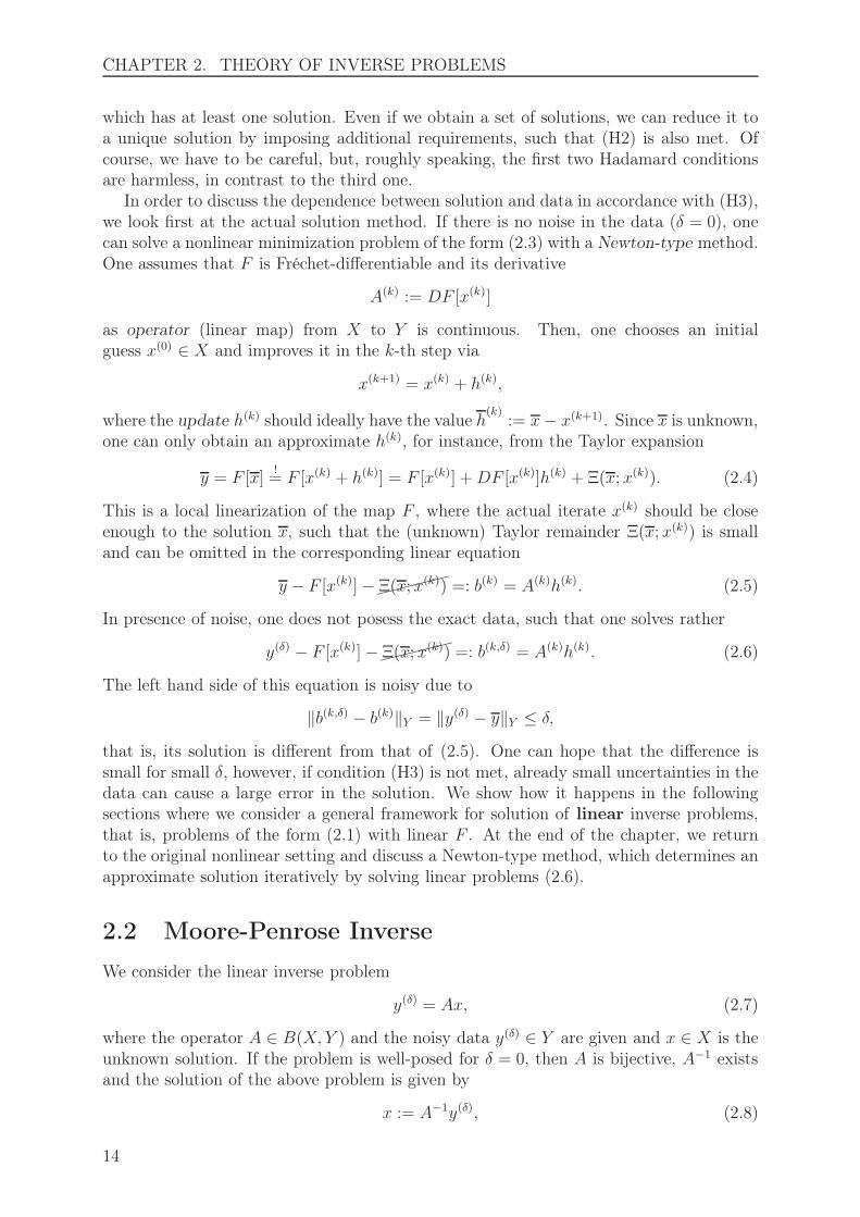
In order to discuss the dependence between solution and data in accordance with (H3),we look first at the actual solution method. If there is no noise in the data (δ = 0), onecan solve a nonlinear minimization problem of the form (2.3) with a Newton-type method.One assumes that F is Fréchet-differentiable and its derivative

A(k) := DF [x(k)]

as operator (linear map) from X to Y is continuous. Then, one chooses an initialguess x(0) ∈ X and improves it in the k-th step via

x(k+1) = x(k) + h(k),

where the update h(k) should ideally have the value h(k)

:= x− x(k+1). Since x is unknown,one can only obtain an approximate h(k), for instance, from the Taylor expansion

y = F [x]!= F [x(k) + h(k)] = F [x(k)] +DF [x(k)]h(k) + Ξ(x; x(k)). (2.4)

This is a local linearization of the map F , where the actual iterate x(k) should be closeenough to the solution x, such that the (unknown) Taylor remainder Ξ(x; x(k)) is smalland can be omitted in the corresponding linear equation

y − F [x(k)]−Ξ(x; x(k)) =: b(k) = A(k)h(k). (2.5)

In presence of noise, one does not posess the exact data, such that one solves rather

y(δ) − F [x(k)]−Ξ(x; x(k)) =: b(k,δ) = A(k)h(k). (2.6)

The left hand side of this equation is noisy due to

‖b(k,δ) − b(k)‖Y = ‖y(δ) − y‖Y ≤ δ,

that is, its solution is different from that of (2.5). One can hope that the difference issmall for small δ, however, if condition (H3) is not met, already small uncertainties in thedata can cause a large error in the solution. We show how it happens in the followingsections where we consider a general framework for solution of linear inverse problems,that is, problems of the form (2.1) with linear F . At the end of the chapter, we returnto the original nonlinear setting and discuss a Newton-type method, which determines anapproximate solution iteratively by solving linear problems (2.6).

2.2 Moore-Penrose Inverse

We consider the linear inverse problem

y(δ) = Ax, (2.7)

where the operator A ∈ B(X, Y ) and the noisy data y(δ) ∈ Y are given and x ∈ X is theunknown solution. If the problem is well-posed for δ = 0, then A is bijective, A−1 existsand the solution of the above problem is given by

x := A−1y(δ), (2.8)

14

2.2. MOORE-PENROSE INVERSE

for all attainable data y(δ), that is, for y(δ) ∈ ran(A). Since A−1 is continuous, this solutionis stable to the noise in the data, as long as the noisy data is attainable. Otherwise, thereare many difficulties on the same way. For instance, if the data y(δ) is not attainable,then y(δ) 6∈ dom(A−1) and A−1y(δ) is not even defined. Thus, we generalize the definitionof “solution”, in order to have any solution. We call an x ∈ X a least-squares solutionof (2.7), if

‖y(δ) − Ax‖Y = infz∈X‖y(δ) − Az‖Y . (2.9)

There is at least one such x, that is, the Hadamard condition (H1) is met. In the well-posedcase where the data is attainable, the unique solution (2.8) would also be a least-squaressolution. However, if A is not injective, that is, if ker(A) 6= 0, we obtain suddenly awhole solution set x+ ker(A). In order to repair the lack of uniqueness, we impose con-straints on the generalized solution. We call x ∈ X a best-approximate solution of (2.7),if x is a least-squares solution of (2.7) and

‖x‖X = inf‖z‖X |z is a least-squares solution of (2.7). (2.10)

One can show that such x is unique, that is, condition (H2) is also fulfilled.The best-approximate solution can also be obtained by the generalization of the term

“inverse” for an operator. The Moore-Penrose inverse A† of A ∈ B(X, Y ) is defined as theunique linear extension of (A|ker(A)⊥)−1 to

dom(A†) := ran(A)⊕ ran(A)⊥

withker(A†) = ran(A)⊥.

If the inverse A−1 exists, we have

A−1A = AA−1 = 1.

Similarly, the Moore-Penrose inverse fulfills the generalized equations

AA†A = A,

A†AA† = A†.

Further, one can show that for all y(δ) ∈ dom(A†), the problem (2.7) has the unique best-approximate solution

x(δ) := A†y(δ) (2.11)

and for x ∈ X, the following statements are equivalent:

• x is a least-squares solution of (2.7),

• x ∈ x(δ) + ker(A),

• x solves the normal equationA∗y(δ) = A∗Ax. (2.12)

This result promises a unique solution for all attainable data. Indeed, the domain ofthe Moore-Penrose inverse is dense in Y . That is, if ran(A) is closed, then the best-approximate solution is obtainable for any data in Y . Moreover, the continuous depen-dence of the solution (2.11) from the data is equivalent to the boundedness of A† and one

15


can show that A† is bounded, if and only if ran(A) is closed. In summary, if this range isclosed, everything is fine.

From now on we assume that the operator A is compact, that is, the sequence (Axn)n∈Nin Y has a convergent subsequence in Y , for each bounded sequence (xn)n∈N in X. Inthis case, which is common for inverse problems, one can show that the range ran(A)is closed, if and only if dim(ran(A)) <∞. That is, in the general case where the rangeis of infinite dimension, the Moore-Penrose inverse A† is unbounded and the Hadamardcondition (H3) is not fulfilled. Even worse, the range of A is “small”, because a compactoperator maps bounded sets (there are “many” bounded sets) to compact sets (there are“few” compact sets). Therefore, the “most” data from Y are not attainable.

The compactness of A allows us to use the singular value decomposition (SVD) –a powerful tool from functional analysis, which provides us an insight into the natureof A† and its domain. Indeed, let (ψ(j), σj, ϕ

(j))j∈N be the SVD of a compact operator A,where σj are the singular values, while ψ(j) and ϕ(j) denote the left and the right singularvectors, respectively. Since (ϕ(j))j∈N is an orthonormal basis of X, any x ∈ X is given by

x =

∞∑

j=1

〈ϕ(j)|x〉Xϕ(j). (2.13)

Further, (ψ(j))j∈N provides an orthonormal basis of ran(A), so that we can write any y inthis range as

y =

∞∑

j=1

〈ψ(j)|y〉Yψ(j).

On the other hand, the singular value expansion of A yields

y = Ax =∞∑

j=1

σj〈ϕ(j)|x〉Xψ(j).

Comparing the coefficients of the two series, we see that

〈ψ(j)|y〉Y = σj〈ϕ(j)|x〉X

and

x =∞∑

j=1

〈ψ(j)|y〉Yσj

ϕ(j)

is a solution to the equation y = Ax. One can show that

x = A†y,

if y ∈ dom(A†), and this is the case, if and only if

∞∑

j=1

|〈ψ(j)|y〉Y |2σ2j

<∞. (2.14)

The latter condition is called the Picard criterion. It says that the best-approximatesolution A†y exists, if and only if the projections 〈ψ(j)|y〉Y of the data decay faster than thesingular values σj . However, the SVD characterizes only A, so, if we have noisy data y(δ),the error projections 〈ψ(j)|y − y(δ)〉Y do not have to decay in the general case. That is,

16


due to the form of the terms |〈ψ(j)|y(δ)〉Y |2σ2j

, the large singular values damp the propagated

noise in x(δ) = A†y(δ), while the small ones amplify it. This allows us to classify inverseproblems – from modestly ill-posed, where the singular values decay polynomially, to theseverely ill-posed, where the decay is exponential.

A similar characterization exists for the case of a finite-dimensional range ran(A).Such inverse problems are evidently well-posed from the theoretical point of view, but inapplications, we observe a behaviour similar to ill-posedness. Consider a linear equation

y(δ) = Ax,

where x ∈ X ≃ Rn, y(δ) ∈ Y ≃ Rm, and A ∈ B(X,Y) ≃ Rm×n is a matrix with rankn < m, that is, A is a compact operator. Theoretically, we can determine the best-approximate solution from the corresponding normal equation

A∗y(δ) = A∗Ax,

because the matrix M := A∗A is invertible due to the full rank of A. But practically, thesolution x(δ) can be meaningless, if the matrix is ill-conditioned, that is, if the conditionnumber

cond(M) := ‖M‖2‖M−1‖2 =σ1σn

is too large. The reason for this are the singular values again – even though they do notconverge to zero, their decay still can be very fast, such that the condition number, asthe ratio between the largest and the smallest singular value, can be very large. From thepractical viewpoint, the Hadamard condition (H3) is not satisfied for such ill-conditionedproblem – the operator A† = M−1A is bounded, but the bound (the norm of the operator)is too large for a meaningful numerical treatment of the above equations. We illustratethis issue on a small linear system.

Example 2.1. “(3× 2)-system”:Let us consider

A =

1 1021 1011 100

, x =

(11

)

, y = Ax =

103102101

and relatively small noise

e =

111

⇒ y(δ) = y + e =

104103102

.

The solution

x(δ) =

(21

)

to the corresponding normal equation is quite wrong, while the residual y(δ) − Ax(δ) isexactly zero. We should not be surprised, because the matrix M = A∗A is ill-conditio-ned – the condition number

cond(M) ≈ 2 · 108

17


as well as the norm of A† = M−1A∗ are quite large. In a nutshell, due to machinearithmetic, the matrix

M =

(3 303303 30605

)

≈(

3 300300 30000

)

is almost singular, the norm ‖A†‖2 is almost infinite and the error

x− x(δ) = M−1A∗e = A†e

arises from the noise amplification due to inversion of M.

The decay of the singular values σj and the corresponding projections 〈ψ(j)|y(δ)〉Y canbe easily compared in a Picard plot. [Hansen-2010] uses this plot in order to deduce a kindof Picard criterion for the finite-dimensional case. Figure 2.1 shows an example of a Picardplot for a certain ill-posed inverse problem. First, one determines the level τ , at which thesingular values level off due to machine arithmetic (see the gap at j ≈ 10). Then, one saysthat the discrete Picard criterion is satisfied, if the ratios |〈ψ(j)|y(δ)〉Y |

σjare (approximately)

non-increasing for all σj > τ . Obviously, this is an analogue of the necessary conditionfor the series in (2.14) to converge. In the Picard plot, we observe that the terms of theseries rather increase for j & 5. That is, the best-approximate solution

x(δ) =16∑

j=1

〈ψ(j)|y(δ)〉Yσj

ϕ(j) (2.15)

is wrong in the last twelve terms. In contrast to (2.14), the discrete Picard criterion carriesa heuristical character and should be used only for sufficiently large n. The length n of thesolution vector can be easily justified in the inverse problems arising from discretizationof an infinite-dimensional problems, as in the following example from [Varah-1983].

0 5 10 15 2010

−30

10−20

10−10

100

1010

1020

1030

j

Singular ValuesProjectionsRatios

Figure 2.1: An example of the Picard plot. Circles represent the singular values σj ,

crosses – the projections |〈ψ(j)|y(δ)〉Y| and diamonds – their ratios |〈ψ(j)|y(δ)〉Y|σj

.

18


0 5 10 15 2010

−5

100

105

1010

t

Figure 2.2: The exact solution (red curve) and the best-approximate solution (blue curve)from Example 2.2.

Example 2.2. “Inverse Laplace transformation”:We consider the linear equation y = Ax, where

(Ax)(s) =

∫ ∞

0

e−stx(t)dt, 0 ≤ s <∞,

describes the Laplace transformation of a function x ∈ L2([0,∞)). The operatorA : L2([0,∞))→ L2([0,∞)) is compact, because its kernel e−st belongs to L2([0,∞)2)(see, for example, [Cheney-2001]). For the fixed exact parameter x(t) := e−t/2, one obtainsthe corresponding exact data

y(s) =1

s+ 12

.

In order to invert the transformation, one solves the above equation numerically bydiscretizing it by means of the Gauss-Laguerre quadrature with certain knots (ti)

ni=1

[Hansen-1994]. After discretization of A and y, the equation turns to an (n× n)-systemy = Ax, where the left hand side differs from Ax. The best-approximate solution iswrong – it has negative values, while the exact solution is strictly positive. In Figure 2.2,we compare the absolute values of the two solutions on the relevant interval. They agreein the vicinity of zero, but their disagreement grows exponentially with t. The reason forthis tremendous discrepancy is the compactness of the operator A. We already studiedthe Picard plot for this inverse problem in Figure 2.1, and this example demonstrates theusefulness of such study. We could foresee that only few terms of the series expansion(2.15) of the solution are trustworthy. Moreover, the rapid decay of the singular valuesclassifies the inverse problem as severely ill-posed and points out that the underlyingoperator is probably compact.

In the above examples, we sketched situations where the Moore-Penrose inverse of acompact operator A is continuous, but the best-approximate solution is worthless. Alsoin the general case, we have Aϕ ≈ 0 for any singular vector ϕ corresponding to a verysmall singular value. That is, instead of the best-approximate solution x(δ), the normalequation yields just a least-squares solution from x(δ) + span(ϕ). It means also that asmall residual norm ‖y(δ) − Ax‖Y does not necessarily imply that x is a good solutionapproximation. This effect can obviously ruin any classical solution method based on

19


the minimization of the residual norm. Therefore, a least squares solution should notbe considered as a proper solution of an ill-posed inverse problem. We should ratheruse a more modern approach, the regularization methods, which denoise (regularize) theMoore-Penrose inverse, so that a meaningful solution can be achieved.

2.3 Regularization

We visualize the regularization of an inverse problem by the diagram in Figure 2.3, wherewe consider the same problem in both ideal and noisy settings. That is, the ideal equationwith exact data does not describe properly the real world, where the data contains noiseand we can only obtain an approximate (and noisy) solution x(δ). The “regularization” is aparametric modification of the noisy equation, which allows to find a unique solution x(λ,δ),which is “near” to x for a proper choice

λ = λ(δ, y(δ)).

Clearly, the regularization can also be applied to the ideal equation, and it is natural todemand a kind of “stability”, in the sense that the regularization of the ideal equationyields a similar solution x(λ), that is,

x(λ,δ) → x(λ), δ → 0.

After coupling these assumptions via

λ(δ)→ 0, δ → 0,

one can expect a kind of “convergence” described by

x(λ,δ) → x, δ → 0.

Noisy

Ideal

y(δ) ≈ Ax(δ) y(δ) = A(λ)x(λ,δ)

y = Ax y = A(λ)x(λ)

“regularization”

“regularization”

noise

“stability”

“convergence”

Figure 2.3: Modifications of an inverse problem and the roles of the noise, stability,regularization and convergence.

20

2.3. REGULARIZATION

This “convergence” does not mean that one can obtain the exact solution x from thenoisy data. The term means that the approximate solution x(λ,δ), no matter how good itis, becomes better as soon as the precision of the data measurement gets better. In thefollowing, we provide mathematical definitions of the concepts we just introduced.

A family (R(λ))λ>0 of operators is called a regularization (of the Moore-Penrose in-verse A†), if

(R1) R(λ) are continuous for all λ > 0,

(R2) R(λ) → A† for λ→ 0 pointwise on dom(A†).

If A is compact, then one can show that ‖R(λ)‖ λ→0−−→∞. Further, if

‖AR(λ)‖ ≤ C, ∀λ > 0, (2.16)

then ‖R(λ)y‖ λ→0−−→∞ for all y 6∈ dom(A†).

Example 2.3. “Truncated SVD”:In the previous section, we motivated that the Moore-Penrose inverse A† cannot handlethe noisy data y(δ) due to the terms in the expansion

A†y(δ) =

∞∑

j=1


ϕ(j), (2.17)

that correspond to the small singular values σj . The simplest way to regularize A† isto truncate the SVD, such that the bad terms do not appear in the series (2.17). Moreprecisely, we define the operator family (R(λ))λ>0 with

R(λ)y(δ) :=

k(λ)∑

j=1


ϕ(j), (2.18)

k(λ) := max

j ∈ N

∣∣∣∣j ≤ 1

λ

.

Evidently, for λ > 1, R(λ) ≡ 0 is continuous, and otherwise, we have

‖R(λ)‖ = 1

σk(λ)<∞, (2.19)

therefore (R1) is fulfilled. Further, according to the Picard criterion, the partial sums ofthe series (2.14) converge for all y ∈ dom(A†), that is,

R(λ)y(δ)λ→0−−→

∞∑

j=1


ϕ(j) = A†y(δ).

Thus, (R2) is satisfied and we conclude that (2.18), called the truncated SVD (TSVD),is a regularization. Moreover, condition (2.16) is fulfilled, because

‖AR(λ)‖ = sup‖y‖Y =1

∥∥∥∥∥∥

k(λ)∑

j=1

〈ψ(j)|y〉Yσj

Aϕ(j)

∥∥∥∥∥∥Y

= sup‖y‖Y =1

∥∥∥∥∥∥

k(λ)∑

j=1

〈ψ(j)|y〉Yψ(j)

∥∥∥∥∥∥Y

≤ sup‖y‖Y =1

‖y‖Y = 1.

That is, the series expansion of A† diverges outside of the domain.

21


Surely, for a fixed λ > 0, the regularized solution x(λ) := R(λ)y depends continuouslyon the data. However, it may happen that the operator R(λ) has not much to do withthe original problem. If we compare the exact solution x = A†y with the more realisticsolution x(λ,δ) = R(λ)y(δ), we can write the total error

x(λ,δ) − x = R(λ)y(δ) − A†y = (R(λ)y − A†y) +R(λ)(y(δ) − y)

as a sum of the regularization error and the propagated noise, respectively. Due to (R2),

‖R(λ)y −A†y‖X → 0, λ→ 0,

that is, we can keep the first term under control by setting the regularization parameter λvery small. Even though R(λ) is bounded, the bound ‖R(λ)‖ may become very large. Inthe general case, the noise y(δ) − y 6∈ dom(A†) and hence, R(λ) amplifies the noise in thesecond term, such that the propagated noise becomes very large,

‖R(λ)(y(δ) − y)‖X →∞, λ→ 0.

For these reasons, we should choose a regularization parameter λ > 0, for that the twoerror terms are in balance (see Figure 2.4).

A function

λ : (0,∞)× Y → (0,∞),

(δ, y(δ)) 7→ λ(δ, y(δ))

is called a parameter choice strategy . A combination ((R(λ))λ>0, λ(δ, y(δ))) of a regulari-

zation with a parameter choice strategy is called a regularization method, if

Rλ(δ,y(δ))y(δ)δ→0−−→ A†y

for all y(δ) with ‖y(δ) − y‖ ≤ δ. In the general case, a parameter choice strategy takesboth the noise level δ and the noisy data y(δ) into account. It can be shown that there isno regularization method where λ depends only on y(δ). The knowledge about the noiselevel δ is so important, that we can provide an example with λ = λ(δ).

10−5

10010

−4

10−2

100

102

λ

Figure 2.4: The regularization error (red curve) and the propagated noise (blue curve)for the problem from Example 2.2 “Inverse Laplace transformation”. The curves are inbalance (white circle) for a certain value of the regularization parameter λ.

22

2.4. TIKHONOV REGULARIZATION

Example 2.4. “TSVD”:The parameter choice strategy λ(δ) := minµ|σk(µ) ≥

√δ yields that for δ → 0,

λ(δ)→ 0 and ‖R(λ(δ))‖δ (2.19)=

δ

σk(λ(δ))≤√δ → 0.

Then, the second term on the right of

‖R(λ(δ))y(δ) − A†y‖X ≤ ‖R(λ(δ))y −A†y‖X + ‖R(λ(δ))‖ · ‖y(δ) − y‖Y

vanishes for δ → 0. The first term also tends to zero due to the property (R2) of theregularization, that is, we have a regularization method.

2.4 Tikhonov Regularization

In this section, we present an intuitive derivation of the Tikhonov regularization. Weremind that in the general case, we solve the linear equation (2.7), where A is a compactoperator with infinite-dimensional range. We already motivated that such an operatoris almost singular, in the sense that the inverses of the operators A and M := A∗A arenot continuous. However, M is a positive semidefinite operator. The basic idea of theTikhonov regularization is to add to M a positively scaled identity, such that the sum

M (λ) :=M + λ21

is far from singular (more regular). More precisely, the operator M (λ) is invertible with acontinuous inverse, that is,

‖(M (λ))−1‖ = 1

λ2

for every value of the regularization parameter λ > 0. This technique is equivalent toreplacing the normal equation (2.12) by

A∗y(δ) =(A∗A + λ21

)x. (2.20)

In order to derive the solutions to the normal equation (2.20), we use the SVD(ψ(j), σj , ϕ

(j))j∈N of the compact operator A. The singular value expansion ofA∗ ∈ B(Y,X) yields

A∗y =∞∑

j=1

σj〈ψ(j)|y〉Yϕ(j),

and

A∗y = (A∗A + λ21)x(2.13)=

∞∑

j=1

(σ2j + λ2)〈ϕ(j)|x〉Xϕ(j)

suggests that the series have equal coefficients. This leads to

σj〈ψ(j)|y〉Y = (σ2j + λ2)〈ϕ(j)|x〉X

and we see that

x =

∞∑

j=1

σ2j

σ2j + λ2

〈ψ(j)|y〉Yσj

ϕ(j)

23


is a solution to the normal equation A∗y = (A∗A+ λ21)x. From this point of view, theTikhonov regularization yields a filtered solution

x(λ,δ) =

∞∑

j=1

χj(λ)〈ψ(j)|y(δ)〉Y

σjϕ(j), (2.21)

where the functions given by

χj(λ) :=σ2j

σ2j + λ2

∈ [0, 1]

ensure that the coefficients of the above series decay properly with respect to the Picardcriterion. At this place, the SVD helps us to interpret the regularization as filtering outthe noisy coefficients, such that an alternative choice of the functions (χj)j∈N also makessense.

Example 2.5. “TSVD”:By setting the filter functions

χj(λ) :=

1, 1 ≤ j ≤ k(λ),0, j > k(λ),

in the regularized solution (2.21), we can derive the TSVD regularization as a special caseof the Tikhonov regularization.

Similar to the TSVD, we can show that the family of operators

R(λ) :=(A∗A+ λ21

)−1A∗ (2.22)

is a regularization of A† and every parameter choice strategy λ(δ) with

λ(δ)→ 0 andδ

λ→ 0, δ → 0

in combination with the Tikhonov regularization (2.22) yields a regularization method.Indeed, since

(A∗A+ λ21)−1A∗ = A∗(AA∗ + λ21)−1,

we obtain

‖R(λ)‖2 = sup‖y‖Y =1

‖(A∗A+ λ21)−1A∗y‖2X

= sup‖y‖Y =1

〈(A∗A + λ21)−1A∗y|(A∗A+ λ21)−1A∗y〉X

= sup‖y‖Y =1

〈A∗(AA∗ + λ21)−1y|A∗(AA∗ + λ21)−1y〉X

≤ sup‖y‖Y =1

(〈(AA∗ + λ21)−1y|AA∗(AA∗ + λ21)−1y〉Y

+ λ2〈(AA∗ + λ21)−1y|(AA∗ + λ21)−1y〉Y)

= sup‖y‖Y =1

〈(AA∗ + λ21)−1y|(AA∗ + λ21)(AA∗ + λ21)−1y〉YCSI≤ sup

‖y‖Y =1

‖(AA∗ + λ21)−1y‖Y · ‖y‖Y

= ‖(AA∗ + λ21)−1‖ = 1

λ2,

24

2.5. PARAMETER CHOICE STRATEGIES

that is, R(λ) is continuous for any λ > 0. Further, for any y ∈ dom(A†) and λ > 0,

‖R(λ)y‖X ≤ ‖R(λ)‖ · ‖y‖Y ≤constλ

is bounded and for λ→ 0, we have

R(λ)y =∞∑

j=1

σ2j

σ2j + λ2

〈ψ(j)|y〉Yσj

ϕ(j) →∞∑

j=1

〈ψ(j)|y〉Yσj

ϕ(j) = A†y,

such that all prerequisites of a regularization are fulfilled. Finally, we estimate the errorvia

‖R(λ(δ))y(δ) −A†y‖X ≤ ‖R(λ(δ))y − A†y‖X + ‖R(λ(δ))‖ · ‖y(δ) − y‖Y ,and let δ → 0. The first term on the right tends to zero due to the above consideration,if λ(δ)→ 0. The second term is bounded,

‖R(λ(δ))‖ · ‖y(δ) − y‖Y ≤1

λδ,

and vanishes, if δλ→ 0. That is, ((R(λ))λ>0, λ(δ, y

(δ))) is a regularization method.

2.5 Parameter Choice Strategies

According to the Tikhonov regularization (or any other regularization), we obtain a wholefamily of possible solutions

x(λ,δ) = R(λ)y(δ), λ > 0.

Intuitively, the regularization parameter should not be too small, otherwise we face theinverted noise again. In the contrary, if we choose a too large λ, then we solve a min-imization problem that has nothing to do with the original one. Let us illustrate thesetwo extreme cases on a familiar finite-dimensional problem.

Example 2.6. “(3× 2)-system”:We resume the simple problem from Example 2.1 and write down the regularized solutionexplicitly,

x(λ,δ) =

(309λ4 + 939λ2 + 36

(3 + λ2)(λ4 + 30608λ2 + 6),

31211λ2 + 6

λ4 + 30608λ2 + 6

)T

.

We see that it vanishes for λ→∞ and tends to x(δ) = (2, 1)T for λ→ 0. Since the exactsolution x = (1, 1)T is given, we can implement a test of all values of λ ∈ [10−10, 105]on a logarithmically equidistant grid. Then, we can find the one optimal λopt, suchthat the distance between x(λopt,δ) and x is minimal (see Figure 2.5). The family ofall regularized solutions defines a curve in R2, and the optimal solution should be theorthogonal projection of the exact solution on this curve. Indeed, for a certain choice ofthe regularization parameter, we reach

x(λopt,δ) ≈ (1, 1)T = x.

Further, we can see that the noise affects primarily the first component of the solution,while a too agressive regularization is able to ruin also the second component.

25


In the general case, it is not clear how to choose the regularization parameter λ, and anyconcrete parameter choice strategy depends on the nature of the actual inverse problem.However, there are some common approaches, from simple and purely heuristic to rigorousand sophisticated. In order to motivate some of them, we consider the normal equation(2.20) in the equivalent formulation as the minimization problem

minx∈X

T (λ,δ)(x), (2.23)

whereT (λ,δ)(x) := ‖y(δ) − Ax‖2Y + λ2‖x‖2X (2.24)

is called the Tikhonov functional. The term ‖x‖2X plays the role of a penalty function,which prevents the noisy components of the solution from growing uncontrollably. In thisregard, the factor λ2 corresponds to the weight of the penalty. If the noise is small, wetrust more in the residual and set λ small (almost no penalty). If the noise is large, weset λ large – the minimization will force the solution x(λ,δ) to be small (damped noisycomponents).

More rigorously, we can show that

d

dλ

(∥∥x(λ,δ)

∥∥2

X

)(2.21)=

∞∑

j=1

d

dλ

(∣∣∣∣χj(λ)


∣∣∣∣

2)

= −∞∑

j=1

σ2j |〈ψ(j)|y(δ)〉Y |2

4λ

(σ2j + λ2)3

< 0.

Therefore, the solution norm is a monotonically decreasing function of λ. Before weanalyze in a similar way the distance between Ax(λ,δ) and the noisy data y(δ) ∈ Y , wenote that the latter is generally not in the range of A. However, Y = ran(A)⊕ ran(A)⊥,such that we can split the data in two parts

y(δ) = y(δ,‖) ∔ y(δ,⊥),

where

y(δ,‖) :=∞∑

j=1

〈ψ(j)|y(δ)〉Y ψ(j)

is the projection of the data on ran(A) and y(δ,⊥) is the part, orthogonal to this projection,that is, 〈y(δ,‖)|y(δ,⊥)〉Y = 0. Then, we can derive that

d

dλ

(∥∥y(δ) − Ax(λ,δ)

∥∥2

Y

)

=d

dλ

∥∥∥∥∥y(δ,‖) + y(δ,⊥) −

∞∑

j=1

χj(λ)〈ψ(j)|y(δ)〉Y ψ(j)

∥∥∥∥∥

2

Y

Pythagoras=

d

dλ

( ∞∑

j=1

∣∣(1− χj(λ))〈ψ(j)|y(δ)〉Y

∣∣2+∥∥y(δ,⊥)

∥∥2

Y

)

=

∞∑

j=1

|〈ψ(j)|y(δ)〉Y |24σ2

jλ3

(σ2j + λ2)3

> 0.

It proves the residual norm to grow monotonically with λ.

26

2.5. PARAMETER CHOICE STRATEGIES

0 0.5 1 1.5 2

0

0.2

0.4

0.6

0.8

1

1.2

λ →∞

λ → 0

Figure 2.5: An illustration to Example 2.6. Black dots represent the regularized solutionsx(λ,δ) for all test values of λ. The red circle is the exact solution x. The blue circle isthe noisy solution x(δ) of the normal equation. The green circle is the optimal solutionx(λopt,δ).

The latter result is used in the Morozov discrepancy principle – a parameter choicestrategy, where the regularization parameter is the solution λ = λMDP of the equation

‖y(δ) − Ax(λ,δ)‖Y = δ. (2.25)

On the one hand, for λ→∞, we have ‖x(λ,δ)‖X → 0 due to (2.21), such that

‖Ax(λ,δ)‖Y ≤ ‖A‖ · ‖x(λ,δ)‖X → 0

and thus

‖y(δ) − Ax(λ,δ)‖Y ≥∣∣‖y(δ)‖Y − ‖Ax(λ,δ)‖Y

∣∣→ ‖y(δ)‖Y

(2.2)≫ δ.

On the other hand, for λ→ 0, we have

x(λ,δ) = R(λ)y(δ) → A†y(δ) = x(δ)

and, since x = x(δ) is a minimizer of the functional ‖y(δ) −Ax‖Y , we obtain

‖y(δ) −Ax(λ,δ)‖Y → ‖y(δ) −Ax(δ)‖Y ≤ ‖y(δ) −Ax‖Y = ‖y(δ) − y‖Y(2.2)

≤ δ.

This functional is continuous, such that the two estimates imply the existence of a solutionof (2.25) and, since the norm grows strictly monotonically with λ, the solution is unique.One can show that the Tikhonov regularization combined with the Morozov discrepancyprinciple yields a regularization method [Groetsch-1993].

27


Residual Norm

SolutionNorm

λ low:ignored noisenoisy solution

λ moderate:denoised solution! λ high:

no noiseno solution

Figure 2.6: An illustration of the L-Curve criterion.

We can also use the monotonicity of the single terms of the Tikhonov functional, inorder to reason that the curve

c(λ) :=

(ln ‖y(δ) − Ax(λ)‖Y

ln ‖x(λ)‖X

)

is the graph of a monotonically decreasing function, which has often a shape of the letterL (see Figure 2.6). Any point on the curve is characterized by the residual and solutionnorms and yields a unique value of the regularization parameter. We already stressed,from the intuitive point of view, how important it is to hit a moderate value λ, whichis not too large and not too small. The L-Curve criterion is a heuristical parameterchoice strategy that sets the regularization parameter λ to the value corresponding to the“corner” of the L-Curve c = c(λ). In terms of the analytical geometry, the corner is thepoint with maximal curvature, that is, the regularization parameter is given by

λLCC := argmaxλ

κ(λ),

κ(λ) :=det(Dc(λ), D2c(λ))

|c(λ)|3 .

Let us show how this simple criterion solves an ill-posed problem we considered earlier.

Example 2.7. “Inverse Laplace transformation”:The heuristical idea of the L-Curve criterion presented in Figure 2.6 is usually not metin practice. Considering the L-Curve for the inverse problem from Example 2.2 (see Fi-gure 2.7), we recognize a “corner”, which corresponds to the choice λLCC ≈ 2 · 10−3. Weobserve also that it is quite close to the optimal value λopt ≈ 4 · 10−2 of the regularizationparameter. The comparison

‖x(δ) − x‖X ≈ 7 · 1016,‖x(λLCC,δ) − x‖X ≈ 1 · 10−1,

‖x(λopt,δ) − x‖X ≈ 6 · 10−3,

28

2.6. NONLINEAR PROBLEMS

10−4

10−2

100

102

10−1

100

101

102

λ →∞

λ → 0

Figure 2.7: The discrete L-Curve (black dots) and the optimal choice (green circle) fromExample 2.7.

shows that the regularized solution is much better than the best-approximate solution.Still, the heuristic of the criterion is coarse and far from optimal with regard to thisproblem.

2.6 Nonlinear Problems

Let us now come back to the nonlinear minimization problem (2.3). Summarizing theconsiderations of the last few sections, a numerical solution method can have the followingform

b(k,δ) := y(δ) − F [x(k)],A(k) := DF [x(k)],

h(k,λ) :=(A(k)∗A(k) + λ21

)−1A(k)∗b(k,δ),

x(k+1) := x(k) + h(k,λ), k ≥ 0, (2.26)

where the regularization parameter λ can be obtained from some parameter choice stra-tegy. This method has a noticeable similarity with the Levenberg-Marquardt method –another Newton-type method, developed for solution of well-posed problems, where δ = 0and y(δ) = y(0) = y actually, but the derivative DF [x(k)] may be an ill-conditioned matrix.If this is the case, one can “trust” in the linearization

minh∈X‖y(0) − F [x(k)]−DF [x(k)]h‖Y

of the problem (2.3) only in a small ball around the iterate x(k). Therefore, one suppliesthe norm to be minimized with a constraint, in order to stay in this ball called the

29


trust region. In other words, one computes the update as a solution h = h(k,λ) of theminimization problem

minh∈X‖y(0) − F [x(k)]−DF [x(k)]h‖2Y + λ2‖h‖2X ,

where the parameter λ justifies the update with respect to the given radius ρ of the trustregion. For instance, the larger the value of λ, the smaller must be the norm ‖h‖2X toensure the minimization of the whole expression above. More precisely,

‖h(k,λ)‖2X = ρ2

must hold. Knowing the corresponding update h(k,λ), one should be able to decide whetherthe next iterate x(k+1) := x(k) + h(k,λ) can be trusted or not. The Armijo-Goldstein crite-rion uses the quotient

µ :=‖b(k,0)‖2Y − ‖y(0) − F [x(k+1)]‖2Y

2〈A(k)h(k,λ)|b(k,0)〉Y(2.27)

to measure the quality of the linearization for the actual iterate. One must provide justtwo parameters 0 < µ1 < µ2 < 1 that describe personal expectations respective linearity.If the function is “not linear enough” (µ < µ1) in the current trust region, one repeatsthe previous step with a smaller radius (a larger λ). Eventually, one can also increase theradius ρ, if the iterate reaches the area, where the function is “pretty linear” (µ > µ2).

While the radius adjustment reminds us on a parameter choice strategy, the above mi-nimization problem is exactly the one we considered for the Tikhonov functional (2.24).Indeed, our regularization method (2.26) can be interpreted as an adaptation of theLevenberg-Marquardt method for ill-posed problems. The choice of the trust region radiustakes place in the Morozov discrepancy principle by choosing λ, such that

‖b(k,δ) − A(k)h(k,λ)‖Y = µ‖y(δ) − F [x(k)]‖Y , (2.28)

where the number 0 < µ . 1 remains constant. The norm on the left is an estimate ofthe residual norm of the next iterate,

‖y(δ) − F [x(k+1)]‖Y ≈ ‖y(δ) − F [x(k)]−DF [x(k)]h(k,λ)‖Y = ‖b(k,δ) − A(k)h(k,λ)‖Y .

Via the parameter µ, we control the reduction rate of the residual norm: for µ near one,we obtain a larger value of λ and correspondingly, a smaller update.

The intuition from the classical Newton-type methods, that the residual norm con-verges monotonically to zero, is not appropriate for an ill-posed problem, where the so-lution does not need to exist, such that a method eventually cannot converge. We couldtry to stop, when the residual norm begins to grow, in which case we risk to experiencethe semiconvergence – the iterates x(k) move towards the exact solution for 0 ≤ k ≤ kstop

and then, for k > kstop, they drift away again (see Figure 2.8). Since we do not know theexact solution, we need a smart stopping rule – a kind of parameter choice strategy thatanalyzes the behaviour of the residuals and decides when the iteration should be stopped.From this point of view, the step number kstop can be seen as a regularization parameter.The residual of our iterative method contains noise of the magnitude δ, that is, intuitively,the method should not minimize the residual norm below that value. We choose kstop asthe minimal k, such that

‖y(δ) − F [x(k)]‖Y ≤ τδ (2.29)

30

2.6. NONLINEAR PROBLEMS

0 2 4 610

−3

10−2

10−1

100

k

Residual Norm

0 2 4 610

−1

100

k

Solution Error Norm

Figure 2.8: Crossing the noise level (dashed line) at kstop = 4, the residual norm (blueline) decays further, but the solution (red line) drifts away.

is fulfilled, where τ ≥ 1 is a safety factor for the case that our noise model is too optimistic.Naturally, we should approach the noise level δ (that is, τ ≈ 1) only with small updates.Thus, by a rule of thumb, we can set the safety factor τ := 1/µ.

The numerical treatment of a nonlinear problem has also a positive effect. We remindthat the map F : X → Y yields data y = F [x] ∈ Y in dependence of the given parame-ter x ∈ X, where x and y are generally elements of some functional spaces X and Y .In practice, all spaces must be reduced to finite dimensions, such that in principle, thedata is a vector y ∈ Rm depending on a finite family of parameters x = (x1, . . . , xn)T .Consequently, the operator DF [x] becomes a matrix A ∈ Rm×n with rank n < m, whichcan be explored by using its SVD (ψ(j), σj , ϕ

(j))nj=1. The right singular vectors (ϕ(j))nj=1

yield an orthonormal basis of Rn, and the singular values (σj)nj=1 give an impression of

the importance of the single basis vectors. The larger the singular value σj , the moreimportant is the corresponding singular vector ϕ(j), the larger is the impact of a variationof the parameter vector x in the direction ϕ(j) on the map value F[x]. In this way, we cansneak into the nature of the (nonlinear) map F in the vicinity of x – the closer is the ℓ-thcomponent of ϕ(j) to one, the easier we can deduce the importance of the parameter xℓfrom the magnitude of the singular value σj . In the general case, the components of asingular vector are mixed and far from one, but if there is 1 ≤ j ≤ n with

σjσ1≈ 1,

|ϕ(j)s |2

‖ϕ(j)‖22≈ 1, (2.30)

we can call the parameter xs strong . Similarly, if there is 1 ≤ j ≤ n with

σjσ1≈ 0,

|ϕ(j)w |2

‖ϕ(j)‖22≈ 1, (2.31)

we can call the parameter xw weak. Further, the matrix Φ = (ϕ(1), . . . , ϕ(n)) ∈ Rn×n

reveals correlations between the parameters (xℓ)nℓ=1. Typically, we are not interested inthe concrete values of the entries (especially for large n), but in their relative magnitudes.Since

|ϕ(j)1 |2 + . . .+ |ϕ(j)

n |2 = 1 ⇒|ϕ(j)

1 |2, . . . , |ϕ(j)n |2 ≤ 1,

31


we prefer to consider the componentwise squared matrix Φ.^2 and represent it as a pic-togram. The entries correspond to blocks in grayscale colors, for instance,

Φ =

1 0 0

0 1/2√3/2

0 −√3/2 1/2

⇒ Φ.^2 =

1 0 00 1/4 3/40 3/4 1/4

=

( )

.

We show in the following example how such pictogram should be interpreted with respectto the definitions (2.30) and (2.31).

Example 2.8. “Singular Value Analysis”:

We consider the matrix

Φ.^2 =

x1x2x3x4x5x6x7

∈ R7×7

of the componentwise squared singular vectors corresponding to an ill-conditioned mat-rix A ∈ R20×7, which arises from discretization of a certain operator DF [x]. For the sakeof simplicity, the parameter of the underlying map F has originally a finite length, thatis, x ∈ R7. The columns of the above pictogram visualize the singular vectors and, for abetter readability, we fade in an additional (zeroth) column with parameters correspondingto the rows. The first column is the most important, its last component is black, thus weconclude that x7 is the strongest parameter in the map F . The second column revealsthat x6 is somewhat weaker than x7. The next two columns show that x4 and x5 areweaker and correlated with each other – a repeated study of these parameters couldimprove the model. The last three columns represent the weakest parameters x1, x2, x3,which are highly correlated – in this case, one can think about excluding these unimportantparameters from the model.

Through the chapter, we explained why only regularization methods can deliver ameaningful solution of an ill-posed problem. Until now we did not discuss under whichconditions they do deliver such solution. The classical Newton-type methods require thatthe derivative DF [x] is Lipschitz continuous (see, for example, [Hanke-Bourgeois-2006]),that is, the Taylor remainder of the linearization (2.4) can be estimated by

‖Ξ(x; x)‖Y ≤ C‖x− x‖2X ,

where C > 0 is constant and x ∈ dom(F ). However, for the ill-posed problem, even thoughthe right-hand side is small (near the solution), the left-hand side can be considerablysmaller, such that the above condition does not describe the local behaviour of the mapproperly and the error of the linearization can go out of control. The usual practice is toreplace the parameter distance by the data distance, that is, to demand

‖Ξ(x; x)‖Y ≤ C‖F [x]− F [x]‖Y

32

2.7. SUMMARY

or‖Ξ(x; x)‖Y ≤ C‖x− x‖X‖F [x]− F [x]‖Y . (2.32)

Under the latter condition, one can show that the Levenberg-Marquardt method (2.26),combined with the parameter choice strategy (2.28) and the stopping rule (2.29), convergesmonotonically [Hanke-1997].

2.7 Summary

So far we made progress only in the mathematical specification of the terms appearingin the key questions of this work. We understand now that an “inversion method” istypically an iterative method for numerical solution of the given inverse problem. In thefollowing, we want to measure the quality of such a method according to its theoreticaland practical properties. Therefore, we formulate these properties as subquestions of theQuestion I (see p. 11), more precisely, from the purely theoretical viewpoint, we can asktwo questions:Question I.1: Does the inversion method contain regularization?

Question I.2: Does the inversion method converge?We already answered the first one for the Levenberg-Marquardt method (2.26), by demon-strating how it is derived by the Tikhonov regularization of the classical Newton method.Moreover, inequality (2.32) is a rigorous condition for the method to converge. Unfortu-nately, we cannot just check this condition for the particular inverse problem presentedin Chapter 1. As we saw, the problem has a complex physical background, such that wecannot treat the corresponding mathematical definition of the map F explicitly. But wecan test our method on some well-studied cases where the solution is already obtained byother means.

33


34

Chapter 3

Application of the Theory

3.1 The Particular Inverse Problem

3.1.1 Functional Spaces

In Chapter 1, we discussed briefly the direct problem of interest and the associated map G,which yields for each interaction potential u the corresponding radial distribution function(RDF). In other words, the particular inverse problem is to solve the equation

y = G[u]

for the given RDF y. Sometimes, the unknown potential u is parameterized via u = H [x],where x is an unknown parameter, and the equation takes the form

y = F [x]

with F := G H. In this chapter, we want to apply the (general) theory of inverseproblems to this particular problem. Even though we never discussed the mathematicalstructure of the sets dom(G) and ran(G), we identified their elements with potentialsand RDFs, respectively, and specified some typical features. That is, a potential was anysmooth function u : (0,∞)→ R that posesses the properties

(U1) limr→0

u(r) =∞,(U2) lim

r→∞u(r) = 0,

(U3) minr∈(0,∞)

u(r) < 0.

We called an RDF any smooth function y : (0,∞)→ (0,∞) with

(Y1) limr→0

y(r) = 0,

(Y2) limr→∞

y(r) = 1,

(Y3) maxr∈(0,∞)

y(r) > 1.

However, the preliminary description of the potentials and RDFs by properties (U1-3)and (Y1-3), respectively, lacks rigorosity from the viewpoints of computer simulation andmathematics. In the following, we discuss the mentioned lack and revise the properties,in order to elaborate more rigorous definitions, which cover our needs.

35

CHAPTER 3. APPLICATION OF THE THEORY

0 2 4 6 80

0.5

1

1.5

2

2.5

3

r

Figure 3.1: A typical RDF.

Figure 3.1 shows a typical RDF y obtained by computer simulation. We see that theproperty (Y1) holds and even more, the number

rcore := maxr > 0|y(s) = 0, ∀s ∈ (0, r]

exists. The reason for this is the strongly repulsive interaction between particles at shortdistances, which is stated by the property (U1) of the underlying potential u. Due torepulsion, each particle has a “core” region (0, rcore], which is rarely entered by otherparticles. Thus, the sampling procedure for the RDF never finds a particle pair at thisshort distance and we observe in simulations, that

y(r) = 0, ∀r ∈ (0, rcore]. (3.1)

In other words, the actual behaviour of the potential in the core region does not matteras long as the repulsion energy is high enough. In principle, this indefiniteness allows usto claim that the singularity of a potential at zero has a polynomial character, that is,1. property of potentials:There exist Ainf

0 , Asup0 ∈ (0,∞), α0 ∈ [0,∞), ∆α0 ∈ [0, α0] and rcore ∈ (0,∞), such that

Ainf0 r

−α0+∆α0 ≤ u(r) ≤ Asup0 r−α0−∆α0 , ∀r ∈ (0, rcore].

This property is particularly useful in the computer simulation, where the values of thepotential cannot be infinite. In the core region, which is a priori never visited by particles,we can replace the potential values by a (very large) constant Ainf

0 = Asup0 while choosing

α0 = ∆α0 = 0. However theoretically, the probability for a short distance between theparticles is not zero, it rather decays exponentially with growing repulsion energy (seeFigure 3.2). Thus, we claim

1. property of RDFs:There exist Binf

0 , Bsup0 ∈ (0,∞), β0 ∈ [0,∞), ∆β0 ∈ [0, β0] and rcore ∈ (0,∞), such that

exp(−Binf

0 r−β0−∆β0)≤ y(r) ≤ exp

(−Bsup

0 r−β0+∆β0), ∀r ∈ (0, rcore].

According to this statement, we observe (3.1) in simulation due to rounding errors in thesampling procedure.

36

3.1. THE PARTICULAR INVERSE PROBLEM

0.88 0.9 0.92 0.94 0.96 0.98

10−4

10−2

100

r

Figure 3.2: A logarithmic plot of the typical RDF (blue dots) near the core region, thatis, for r → rcore + 0. The black line represents the corresponding linear fit of the points.

Figure 3.3 shows a typical potential u used to describe the nonbonded interactions ina fluid. We confirm the property (U2) and even more, we see that u(r) ≈ 0 for finitelylarge distances. This approximation is used in the computer simulation, in order to reducethe computational effort in a large system. Cutting off the potential at some appropriatedistance rcut <∞ and continuating it with zero allows to consider only interactions insmall subregions of the system. However, the resulting uncertainties in the energy andthe pressure can only be estimated and corrected, if the convergence of the potential tozero is fast enough (see Appendix B). Such potentials are called short-ranged and theLennard-Jones potential is one of them. In this work, we do not consider electrostaticinteractions between particles, because they are modeled by the Coulomb potential, whichis long-ranged. Therefore, we claim that our potentials are short-ranged:2. property of potentials:There exist A∞ ∈ (0,∞), α∞ ∈ (d,∞) and rcut ∈ (rcore,∞), such that

|u(r)| ≤ A∞r−α∞ , ∀r ∈ (rcut,∞).

This model also covers the case where the potential is cut off.

0 2 4 6 8−1

−0.5

0

0.5

1

r

Figure 3.3: A typical nonbonded interaction potential.

37


As the property (Y2) states, the RDF has a similar asymptotic behaviour – it convergesto one for large distances. We see in Figure 3.1 that the deviations of the function’sextremal values from the limit decay very fast and become vague due to the statisticalnoise as the distance grows. We can model the decay on the interval (rcut,∞) polynomially

|y(r)− 1| ≤ r−βpoly∞

or exponentially|y(r)− 1| ≤ exp

(

−rβexp∞

)

.

Obviously, the first version is a safer estimate, no matter how large the power is. Regardingthe good correspondence between RDF and potential promised by Henderson theorem, weexpect that the power of the polynomial estimate is comparable with the number d = 3of dimensions, like in the 2. property of potentials. We plot the power as a function ofthe distance

βpoly∞ (r) ≈ − ln(|y(r)− 1|)

ln(r)

and observe that the mentioned decay becomes faster with growing r (see Figure 3.4).Even more, for large r, the power reaches the desired level near d. Probably, we cannotobserve βpoly

∞ > d just because the data has finite length and becomes noisy in the lastcomponents. The best polynomial fit confirms our hypothesis. Therefore, we claim thatin the absence of noise, the convergence has the polynomial behaviour:2. property of RDFs:There exist B∞ ∈ (0,∞), β∞ ∈ (d,∞) and rcut ∈ (rcore,∞), such that

|y(r)− 1| ≤ B∞r−β∞, ∀r ∈ (rcut,∞).

Finally, we discuss the shape of the potential well, which is essential for attractionbetween particles in a fluid. The term “fluid” covers both liquids (high density) and gases(low density). At high density, the particles are kept together by pressure, such thatinteractions are mainly repulsive. However, if we simulate a liquid at moderate density

0 2 4 6 8 101.5

2

2.5

3

3.5

r

Figure 3.4: The power βpoly∞ (r) (blue dots) and the best polynomial fit (black line).

38


and without attractive forces, the particles could diffuse to the whole container (like agas), which would be unusual for a liquid. Roughly speaking, the particles try to minimizethe energy, such that the potential should have a well, which defines a preferred distance,as we indicated in the property (U3) and specify now:

3. property of potentials:There exists a unique rmin ∈ (rcore, rcut], such that

−∞ < u(rmin) = minr∈(0,∞)

u(r) < 0.

Due to this attractive feature of the interaction, the sampling procedure for the RDFcounts very many neighbours in a relatively small layer around a reference particle. Theconsequence is, as the property (Y3) states, that a noticeable peak emerges in the his-togram:3. property of RDFs:There exists a unique rpeak ∈ (rcore,∞), such that

1 < y(rpeak) = maxr∈(0,∞)

y(r) <∞.

In the above discussion, we developed new formal properties describing the sets ofpotentials and RDFs. While some old properties remained, other were generalized orspecified, but both the old and the new descriptions have a nearly equivalent physicalinterpretation. However, the corresponding mathematical statements are not equivalent,especially, the constants α0 and β0 establish the accurate behaviour of the functions nearzero. We summarize the results of our study in the following definitions.Definition:For any α0 ∈ [0,∞) and ∆α0 ∈ [0, α0], let the set SU(α0,∆α0) contain all piecewisesmooth functions u : (0,∞)→ R with the following properties:

(SU1) there exist Ainf0 , A

sup0 ∈ (0,∞) and rcore ∈ (0,∞), such that

Ainf0 r

−α0+∆α0 ≤ u(r) ≤ Asup0 r−α0−∆α0, ∀r ∈ (0, rcore], (3.2)

(SU2) there exist A∞ ∈ (0,∞), α∞ ∈ (d,∞) and rcut ∈ (rcore,∞), such that

|u(r)| ≤ A∞r−α∞ , ∀r ∈ (rcut,∞), (3.3)

(SU3) there exists a unique rmin ∈ (rcore, rcut], such that

−∞ < u(rmin) = minr∈(0,∞)

u(r) < 0. (3.4)

We call an element of the set

SU :=⋃

α0≥0

⋃

∆α0≤α0

SU(α0,∆α0) =⋃

α0≥0

SU(α0, α0)

a potential.

39


Definition:For any β0 ∈ [0,∞) and ∆β0 ∈ [0, β0], let the set SY (β0,∆β0) contain all piecewisesmooth functions y : (0,∞)→ (0,∞) with the following properties:

(SY1) there exist Binf0 , Bsup

0 ∈ (0,∞) and rcore ∈ (0,∞), such that

exp(−Binf

0 r−β0−∆β0)≤ y(r) ≤ exp

(−Bsup

0 r−β0+∆β0), ∀r ∈ (0, rcore], (3.5)

(SY2) there exist B∞ ∈ (0,∞), β∞ ∈ (d,∞) and rcut ∈ (rcore,∞), such that

|y(r)− 1| ≤ B∞r−β∞, ∀r ∈ (rcut,∞). (3.6)

(SY3) there exists a unique rpeak ∈ (rcore, rcut], such that


y(r) <∞. (3.7)

We call an element of the set

SY :=⋃

β0≥0

⋃

∆β0≤β0

SY (β0,∆β0) =⋃

β0≥0

SY (β0, β0)

a radial distribution function (RDF).

Even though the definitions are strictly derived from their physical motivation, thesets SU and SY do not suffice for a mathematically rigorous discussion of the problem.For instance, if we intend to solve the problem by the Levenberg-Marquardt method pre-sented in the previous chapter, then each set should be embedded in a Hilbert space, say,SU → U and SY → Y . Especially, the method makes use of the derivative DG ∈ L(U, Y )of G : U → Y , but its definition via

DG[u] := limt→0

1

t

(

G[u+ tv]−G[u])

, u, v ∈ U,

makes sense only for linear spaces U and Y . Each of the sets SU(α0,∆α0) of potentialsalready posesses some structure, namely

u, υ ∈ SU(α0,∆α0), c > 0 ⇒ u+ υ, cu ∈ SU(α0,∆α0),

but none of them is a linear space. Likewise, none of the sets SY (β0,∆β0) is a linearspace, because all RDFs converge to one at infinity. Further, we have to supply eachspace with an appropriate norm ‖ · ‖, in order to justify the common definition of theterm “limit” via

a = limk→∞

a(k) :⇔ limk→∞‖a− a(k)‖ = 0,

and to measure the quality of the iterates and of the approximate solution. A popularnorm in the physical literature is the root mean square distance given by

RMSD(f) :=

(∫

|f(r)|2dr)1/2

for a function f . However, the integral diverges for y ∈ SY (β0,∆β0) due to (3.6) andfor u ∈ SU(α0,∆α0), 0 < ∆α0 < α0, due to (3.2). Even for u ∈ SU(0, 0), the most part

40


of RMSD(u) <∞ comes from the integration over the core region where the potentialvalues are apparently unimportant. In other words, the norms for potentials and RDFsneed at least a fair reweighting. A popular approach in functional analysis is to embeda set into a weighted Lebesgue space L2((0,∞), w), where w ∈ C∞(0,∞) is a boundedweight function. This space is a Hilbert space of all measurable functions f : (0,∞)→ R

that are square-integrable with the weight w, that is, ‖f‖ <∞. The norm is induced bythe weighted inner product

〈f |g〉 :=∫ ∞

0

f(r)g(r)w(r)dr

defined for any functions f and g from the Hilbert space.

Theorem A1:SU is a subset of the weighted Lebesgue space U := L2((0,∞), wU), if wU ∈ C∞((0,∞))is a bounded weight function, such that

limr→0

u(r)2wU(r) = 0, (3.8)

limr→∞

wU(r) = 1, (3.9)

for any u ∈ SU .

Proof: Let u ∈ SU(α0,∆α0) be arbitrary. According to (3.8), there exists r0 ∈ (0, rcore]with

|u(r)2wU(r)| ≤ 1, ∀r ∈ (0, r0),

because u, wU ∈ C∞(0, rcore). Then, we have∣∣∣∣

∫ r0

0

u(r)2wU(r)dr

∣∣∣∣≤∫ r0

0

|u(r)2wU(r)|dr ≤ r0 ≤ rcore <∞.

Further, due to (3.3), there exist A∞ ∈ (0,∞), α∞ ∈ (d,∞) and rcut ∈ (rcore,∞) with

|u(r)| ≤ A∞r−α∞ , ∀r ∈ (rcut,∞).

Moreover, according to (3.9), we can assume that r1 ∈ (rcut,∞) exists with

|wU(r)| ≤ 2, ∀r ∈ (r1,∞).

Thus, we have∣∣∣∣

∫ ∞

r1

u(r)2wU(r)dr

∣∣∣∣≤

∫ ∞

r1

|u(r)2wU(r)|dr

≤ 2A∞

∫ ∞

r1

r−2α∞dr

= 2A∞1

−2α∞ + 1r−2α∞+1

∣∣∣∣

∞

r1

= 2A∞1

2α∞ − 1r−2α∞+11 <∞.

41


Finally, since u and wU are bounded on the interval (r0, r1), we have

|u(r)2wU(r)| ≤ C, ∀r ∈ (r0, r1)

for a constant C <∞, that is,∣∣∣∣

∫ r1

r0

u(r)2wU(r)dr

∣∣∣∣≤ C(r1 − r0) <∞.

Summarizing the above estimates, we obtain

‖u‖2U =

∣∣∣∣

∫ ∞

0

u(r)2wU(r)dr

∣∣∣∣

≤∣∣∣∣

∫ r0

0

u(r)2wU(r)dr

∣∣∣∣+

∣∣∣∣

∫ r1

r0

u(r)2wU(r)dr

∣∣∣∣+

∣∣∣∣

∫ ∞

r1

u(r)2wU(r)dr

∣∣∣∣<∞,

that is, u ∈ U .

Theorem A2:SY is a subset of the weighted Lebesgue space Y := L2((0,∞), wY ), if wY ∈ C∞((0,∞))is a bounded weight function, such that

|wY (r)| ≤ C1r−β, ∀r > r∞, (3.10)

for certain C1 ∈ (0,∞), β ∈ (1,∞) and r∞ ∈ (0,∞).

Proof: Let y ∈ SY (β0,∆β0) be arbitrary. According to (3.6), we can assume

|y(r)| ≤ 2, ∀r > r∞,

without loss of generality. Then, we have∣∣∣∣

∫ ∞

r∞

y(r)2wY (r)dr

∣∣∣∣≤ 4

∫ ∞

r∞

|wY (r)|dr(3.10)

≤ 4C1

∫ ∞

r∞

r−βdr

= 4C11

−β + 1r1−β

∣∣∣∣

∞

r∞

= 4C11

β − 1r1−β∞ <∞.

Finally, since y and wY are bounded on the interval (0, r∞), there exists a constantC2 ∈ (0,∞) with

|y(r)2wY (r)| ≤ C2, ∀r ∈ (0, r∞),

that is ∣∣∣∣

∫ r∞

0

y(r)2wY (r)dr

∣∣∣∣≤ C2r∞ <∞.

Summarizing the above estimates, we obtain

‖y‖2Y =

∣∣∣∣

∫ ∞

0

y(r)2wY (r)dr

∣∣∣∣≤∣∣∣∣

∫ r∞

0

y(r)2wY (r)dr

∣∣∣∣+

∣∣∣∣

∫ ∞

r∞

y(r)2wY (r)dr

∣∣∣∣<∞,

42


that is, y ∈ Y .

In this work, we use the weight functions

wU(r) := exp

(

−1r

)

, (3.11)

wY (r) := exp(−r), (3.12)

which satisfy the requirements of the theorems A1 and A2, respectively. These functionsestablish norms and limits on the spaces U and Y . It remains to discuss the structureof the set SX of possible interaction parameters. Disregarding the concrete parameteri-zation H , there are typically only few parameters, which are positive, such that we canembed SX := (0,∞)n into the Euclidean space X := Rn for some finite n ∈ N. X is aHilbert space with the standard inner product

〈x|ξ〉X := 〈x|ξ〉2 =n∑

j=1

xjξj , ∀x, ξ ∈ X.

Following the above considerations, we work with the map

F : XH−→ U

G−→ Y

and write the particular inverse problem in the usual form as equation

y = F [x], (3.13)

where x ∈ X is the unknown exact parameter vector and y ∈ Y is the given exact data(RDF). In the future discussions, we will occassionally consider the inverse problem

y = G[u], (3.14)

where the unknown exact potential u ∈ U appears without being parameterized.

3.1.2 Inversion Method

We explained earlier why an inverse problem of the form (3.13) is ill-posed in practice,for instance, if we do not know the exact data y. This is the case for our problem – wehave only the noisy RDF y(κ) measured experimentally with a certain noise level κ > 0,that is,

‖y(κ) − y‖Y ≤ κ.

Further, there are always model errors, for example, G does not perfectly describe theRDF as a physical quantity, and the parameterization H or the space U are not goodenough to represent an interaction potential. In other words, it may happen that thereis no x ∈ X with u = H [x] or no u ∈ U with y = G[u]. Finally, the exact maps G and Fare not available – we have only the approximate computational implementations G(ν)

and F (ν) := G(ν) H , such that

‖G(ν)[u]−G[u]‖Y ≤ ν (3.15)

holds for a certain ν > 0. Therefore, our inverse problems become

y(δ) = F (ν)[x], (3.16)

y(δ) = G(ν)[u], (3.17)

43


where we assume that the noise level δ takes into account all uncertainties of our model,that is, δ := κ + ν and y(δ) := y(κ).

We already discussed in Chapter 2 ill-posed problems of the above form and presentedthe Levenberg-Marquardt method (2.26) as a good numerical solution approach. However,due to the chosen functional spaces U and Y , we have to take a closer look on the normalequation corresponding to the inverse problem (3.17). Simplifying our usual notationsto b := y(δ) −G[u] and A := DG[u] in this paragraph, we see that the update h to theactual approximate potential u fulfills

(A∗A + λ21)h = A∗b

for some λ > 0. Here, A∗ : Y → U is the adjoint operator to A : U → Y with respect tothe inner products of the weighted Lebesgue spaces U and Y , and it is defined by

〈Au|y〉Y = 〈u|A∗y〉U .

The resulting operator differs from the usual L2((0,∞))-adjoint operator A∗2 , which is aninfinite-dimensional analogon of a transposed matrix. For A∗2 , it rather holds

〈Au|y〉L2((0,∞)) = 〈u|A∗2y〉L2((0,∞)),

but its relation to A∗ can be derived. Introducing the multiplication operators

WU : L2((0,∞))→ L2((0,∞)), u 7→ wUu,

WY : L2((0,∞))→ L2((0,∞)), y 7→ wY y,

we obtain on the one hand,

〈AWUu|y〉Y = 〈AWUu|WY y〉L2((0,∞)) = 〈WUu|A∗2WY y〉L2((0,∞)) = 〈u|A∗2WY y〉U ,

that is, (AWU)∗ = A∗2WY . On the other hand, the equality

〈AWUu|y〉Y = 〈WUu|A∗y〉U = 〈WUu|WUA∗y〉L2((0,∞)) = 〈u|WUA

∗y〉U

reveals that (AWU)∗ = WUA

∗. Due to the uniqueness of the adjoint operator, we have

WUA∗ = A∗2WY

and by multiplying the normal equation with WU from the left, we obtain

(A∗2WYA+ λ2WU1)h = A∗2WY b,

what is more suitable for further discretization and implementation. This modified equa-tion can also be used for problem (3.16). WU then corresponds to the (non-present)weighting of the space X and can be omitted.

In order to implement the Levenberg-Marquardt method on the computer, we writeit for finite-dimensional spaces, that is, we discretize the participating functions. Dis-cretization is quite natural for our inverse problem, because experiments usually providethe data y(δ) on some equidistant grid

ri := i∆r, 1 ≤ i ≤ m,

44


with a grid step ∆r > 0. Thus, any data is actually a vector from the set

SY := y ∈ Rm| yi = y(ri), y ∈ SY , 1 ≤ i ≤ membedded in the space Y := Rm with the inner product

⟨y(1)|y(2)

⟩

Y:= ∆r

m∑

i=1

y(1)i y(2)

i wY (ri) = ∆r⟨y(1)|WY y(2)

⟩

2,

WY := diag(wY (r1), . . . , wY (rm)).

Conveniently, we use the same grid for the underlying potential by writing it as a vectorfrom the set

SU := u ∈ Rm| ui = u(ri), u ∈ SU , 1 ≤ i ≤ membedded in the space U := Rm with the inner product

⟨u(1)|u(2)

⟩

U:= ∆r

m∑

i=1

u(1)i u(2)

i wU(ri) = ∆r⟨u(1)|WUu(2)

⟩

2,

WU := diag(wU(r1), . . . , wU(rm)).

The space of parameters is already finite-dimensional and we define

SX := SX = (0,∞)n → X := X = Rn, 〈·|·〉X := 〈·|·〉X = 〈·|·〉2.The discretization of the maps between these spaces is obvious and leads to the discreteinverse problems

y(δ) = F(ν)[x], (3.18)

y(δ) = G(ν)[u]. (3.19)

The Levenberg-Marquardt method solves (3.18) by linearization, which requires dis-cretization of the operator A(k) that represents the derivative of the RDF with respect tothe parameter. In Chapter 1, we mentioned the complexity of the formal expression forthe RDF and naturally, its derivative shows even more complexity. That is, while everyserious software package (GROMACS, ESPResSo++, NAMD etc.) can run a molecularsimulation and obtain the corresponding RDF from the snapshots of the systems tra-jectory, a computational procedure for the derivative is not included there by default.Therefore, we prefer to use a solution algorithm with a lower requirement – the ability tosolve the direct problem, that is, to compute an RDF for the given interaction potential.Consequently, in our method, we discretize the operator D itself by approximating thederivative DF (ν) by finite differences

DjF(ν)i [x] :=

F(ν)i [x +∆xje(j)]− F(ν)

i [x]∆xj

, 1 ≤ i ≤ m, 1 ≤ j ≤ n,

where the components of the variation vector ∆x ∈ Rn should be justified according tothe following consideration. On the one hand, the map F(ν) is still noisy:

‖F(ν)[x]− F(ν)[ξ]‖Y = ‖F(ν)[x]− F(ν)[ξ] + F[x]− F[x]

+F[ξ]− F[ξ]‖Y≤ ‖F[x]− F[ξ]‖Y + ‖F(ν)[x]− F[x]‖Y

+‖F[ξ]− F(ν)[ξ]‖Y(3.15)

≤ ‖F[x]− F[ξ]‖Y + 2ν,

45


so we have to choose ∆xi large enough to guarantee that the actually important informa-tion, F[x]− F[ξ], does not disappear in the noise of magnitude 2ν. On the other hand, thevariations should be small enough to take the local behaviour of F(ν) into account. In thesecircumstances, we make a compromise by imposing the following variation condition,

2ν < ‖F(ν)[x +∆xje(j)]− F(ν)[x]‖Y < 4ν, (3.20)

which should provide a reasonable choice of the variation vector ∆x. In our iterativeregularization method, we ignore small perturbations in the operator A(k), consider thedifference between discretizations of DF and DF (ν) as negligible and take

A(k) := DF(ν)[x(k)].

Since the number ν is an important part of the variation condition, we have to modelthe noise in the map F(ν) in a way, which allows us to estimate the noise level. Weassume that each component F(ν)

i of the noisy map is normally distributed with mean Fiand standard deviation η2i . The mean RDF F is unknown, but we can estimate thevector η ∈ Rm of standard deviations in each step from ten samples of the map F(ν) viathe sample variance

η2i = Var[F(ν)i ], 1 ≤ i ≤ m.

Then, the noise level ν can be estimated by using the properties of the sample mean via

ν2 ≈ E[

‖F(ν)[x]− F[x]‖2Y

]

=m∑

i=1

E[

|F(ν)i [x]− Fi[x]|2

]

wY (ri)∆r

=m∑

i=1

Var[F(ν)i ]wY (ri)∆r

= ‖η‖2Y. (3.21)

According to the above discussion, the Levenberg-Marquardt method takes the form

b(k,δ) := y(δ) − F(ν)[x(k)],

A(k) := DF(ν)[x(k)],

h(k,λ) :=(

A(k)∗2WY A(k) + λ21)−1

A(k)∗2WY b(k,δ),

x(k+1) := x(k) + h(k,λ), k ≥ 0, (3.22)

for the inverse problem (3.18), and

b(k,δ) := y(δ) −G(ν)[u(k)],

A(k) := DG(ν)[u(k)],

h(k,λ) :=(

A(k)∗2WY A(k) + λ2WU

)−1

A(k)∗2WY b(k,δ),

u(k+1) := u(k) + h(k,λ), k ≥ 0, (3.23)

for the inverse problem (3.19). In this chapter, we always assume that x(0), u(0), y(δ), νand δ are given or can be estimated, such that the regularization parameter λ can bechosen via the Morozov discrepancy principle (2.28) and the iteration can be terminateddue to the stopping rule (2.29).

46


3.1.3 Direct Problem

Since our inversion method’s primary requirement is the ability to solve the direct prob-lem, we briefly address the subtleties of the computer simulation, where the RDF iscomputed from the underlying potential or its parameters. For instance, in Chapter 1,we explained that it is done by molecular dynamics, which moves the particles of a fluidin accordance with the Newton equations. The corresponding solution method must beenergy-conserving, otherwise the particles are either accelerated until the system blowsup (due to energy gain), or slowed down until the system freezes (due to energy loss).But, in an experiment, where a total energy conservation is nearly impossible, the RDFis usually measured rather at constant temperature than at constant energy. Therefore,all our simulations are performed in the canonical ensemble (also called NV T -ensemble),that is, for fixed number N of particles, volume V and temperature T of the system. Thesource term of the Newton equations can be extended with a thermostat – a friction force,which speeds up or slows down the particles, such that the temperature remains constant(see Appendix B.1).

On the other hand, the parameters N , V and T allow a completely statistical descrip-tion of the system by a distribution of particles, where their actual trajectories do notmatter. This distribution is based exclusively on these three parameters and the inter-action potential, and totally determines the fluid’s statistical properties, including theRDF. Therefore, disregarding the popularity of the molecular dynamics in the physicalcommunity, a computer simulation can also be performed via the Monte Carlo method,which describes the fluid directly from the statistical viewpoint (see Appendix B.1). In anutshell, the method picks out in each step a random particle, moves it slightly along arandom vector, determines the change in the energy and depending on the temperature,decides whether this change is compatible with the canonical distribution (step accepted)or not (particle is moved back). Evidently, one can implement this procedure much easierthan the molecular dynamics, therefore we use the Monte Carlo method in our preliminarytests in the next section.

A further subtlety we want to discuss here are the units used in a computer simulation.In the literature, one can find the tabulated RDF accompanied by all necessary experi-mental settings, including the temperature T in [K] and the density ρ := N

Vin [Å

−3].

Considering that, in SI units, we have

1 [Å] = 10−10 [m],

it is clear that no numerical method should work with numbers of that order. One usuallyintroduces the reduced units by setting a unit mass Munit, a unit length σunit and a unitenergy εunit. Then, the computer simulation works with the more suitable quantities

T ∗ =kBT

εunit,

ρ∗ = ρ(σunit

)3,

ε∗ =ε

εunit,

σ∗ =σ

σunit,

which are all of the same order and nearly equal to one. We often omit the stars, becausewe always mean the reduced units, unless we specify other units.

47


ρc ρt ρ

T c

T t

T

G L S

F

Figure 3.5: Phase diagram of a simple fluid.

Finally, let us take a look inside the physics of the simulation, in order to understandhow the parameters T and ρ are to set up. We explained in Chapter 1, that a fluid is asystem of particles, which are moved according to the given interactions. Even thoughthe particles of a solid also interact, moving particles would be quite unusual – intuitively,a solid system is either too cold or too dense to flow. Indeed, solid and fluid are differentphase states of matter, where fluid is a generic term for liquid and gas. Figure 3.5shows the phase diagram, which helps to distinguish between different phase states. Insuch diagram, the temperature T and the density ρ of the system determine the state ofmatter (G stands for gas, L for liquid, S for solid, F for fluid). The solid lines representthe coexistence lines, where two phase states are present simultaneously. The green circleat (ρt, T t) designates the triple point, where all three states are present. The red circleat (ρc, T c) stands for the critical point, where a part of the matter is in the gaseousstate and another part in the liquid state. The dashed line just separates visually thesupercritical fluid from the other fluid states. We use the phase diagram as a guide forsetting up a simulation in the NV T -ensemble. While we can carefree simulate a gas ora liquid, we avoid the solid state as well as the coexistence lines by choosing appropriatetemperature and density. The safest for simulation is the supercritical fluid, therefore weprefer this phase state in the following section.

3.2 Simulated Data for Two-dimensional Fluids

Before we apply our regularization method on a real-world (ill-posed) inverse problem, wewant to test it first under better conditions. We wrote our own code for two-dimensionalmolecular simulations, in order to quickly obtain insight into the dependence between theRDF and the underlying interaction potentials. We combined the programming languagesC++ and Perl to implement the Monte Carlo and the Levenberg-Marquardt methods,which solve the direct and the inverse problems, respectively. For each inverse problem,we choose a certain exact solution x and use y(ν) := F(ν)[x] as the given data. Since themeasurements become preciser (ν smaller) for a larger number N of particles, we findthat N = 128 is an acceptable value. Surely, a simulated RDF contains some statistical

48

3.2. SIMULATED DATA FOR TWO-DIMENSIONAL FLUIDS

noise, as modeled by the noisy map F(ν), but its magnitude is so small that we can considerthe data y(ν) as nearly exact and the inverse problem as well-posed. We remind that suchproblem still can be ill-conditioned, as we demonstrated earlier in Chapter 2.

The preliminary formulation of the inverse problem was to obtain the Lennard-Jonesparameters (ε and σ) as well as the temperature T and the density ρ for a simple fluid ofmonatomic molecules. However, after we test few possible norms for the data (Lebesgue,Sobolev, eventually weighted with characteristic functions), the derivative DF(ν)[x] revealsa correlation between the parameters. Indeed, it is one aspect of the direct problem – εand σ can be chosen as the energy/temperature scale and the length/density scale, respec-tively. It is intuitively clear because of the reduced units, where we can choose εunit := εand σunit := σ, such that ε∗ = σ∗ = 1. We show this more rigorously in Theorem P7 inAppendix A.4. For this reason, we prefer to set ε = σ = 1 at this stage of testing andconsider x = (ρ,T)T as the basic parameters of the fluid.

In the first test, we want to know whether the parameters can also be obtained fromthe RDF, if the method starts with a very bad initial guess x(0) far from the exact solu-tion x = (ρ,T)T . We choose x from an equidistant grid on the area [0.2, 0.9]× [0.8, 2] andalways use x(0) := (0.55, 1)T as the initial value. Since

(ρc,Tc) ≈ (0.35, 0.5),

(ρt,Tt) ≈ (0.8, 0.4),

for the two-dimensional Lennard-Jones fluid [CM-1992], the test area corresponds to the(supercritical) fluid state, including the vicinity of the fluid-solid coexistence line (see againFigure 3.5). In order to solve the inverse problem, we combine the Levenberg-Marquardtmethod and the “pure” (and fast) Newton method where the regularization parameter iszero. We observe that the noise has no significant influence on the iterates x(k) as long as

‖y(ν) − F(ν)[x(k)]‖Y ≫ ν

holds. For these iterates, there is no need for regularization, until they reach the areawhere the residual norm is of nearly the same order as ν and the (slower) Levenberg-Marquardt method finds a better application. In few steps, we obtain the parametersfrom the test area with relative errors

( |ρ− ρ||ρ| ,

|T− T||T|

)T

≈ (2.3 · 10−3, 8.1 · 10−3)T ,

what is a nearly perfect reconstruction.Already during these first numerical solutions of the inverse problem, we observe some

useful facts, which allow to simplify the application of the Levenberg-Marquardt methodin the following:

• The variations ∆x, which are necessary for the numerical differentiation and mustfulfill the condition (3.20), can be chosen constant.

• The noise in the map F(ν) is nearly constant in the whole test area, such that wecan choose a uniform bound ν for the noise there.

• For any initial guess, the Newton method is able to move the iterates close enoughto the exact solution, such that the Levenberg-Marquardt method can take over.

49


Further, investigating the impact of the parameter variations on the RDF, we discoverthat for x near the fluid-solid coexistence line, it holds that

∥∥∥F(ν)

[x + |∆ρ|e(1)

]− F(ν)[x]

∥∥∥Y

≫∥∥∥F(ν)

[x− |∆ρ|e(1)

]− F(ν)[x]

∥∥∥Y

.

In other words, the RDF is sensitive to the fluid-solid phase transition. For this reason,we keep the temperature and the density as parameters of the RDF in the following tests.In experiments, the data is usually measured near the triple point, thus we set the densitynear the mentioned coexistence line, but definitely in the fluid state. In this fashion, wehope to obtain representative results even in this very simple, preliminary setting.

The second test concerns a fluid of diatomic homonuclear molecules with the bondlength ℓ. For the sake of simplicity, we assume that the bond is rigid and obtain theparameter x = (T, ρ, ℓ)T with relative errors near

(1.5 · 10−4, 4.1 · 10−3, 9.3 · 10−4)T .

Inspired by the high quality of this reconstruction, we decide to extend the model tox = (T, ρ, ℓ, kℓ)T by considering the bond as a flexible spring with stiffness kℓ. However,we observe that ∥

∥∥F(ν)

[x +∆kℓe(4)

]− F(ν)[x]

∥∥∥Y

. 2ν

for any variation ∆kℓ, such that we cannot determine the corresponding derivative of F(ν)

reliably. We discussed this situation more generally in Chapter 2, where we stressed thateven in a well-posed, finite-dimensional problem, an ill-conditioned matrix can occur. Ifthe influence of a parameter on the map is so small, that the variation condition is fulfilledonly for very large variation, if ever, then the matrix DF(ν) is close to singular, as we cansee in this concrete example,

‖D4F(ν)[x]‖Y =‖F(ν)[x +∆kℓe(4)]− F(ν)[x]‖Y

|∆kℓ|.

2ν

|∆kℓ||∆kℓ|→∞−−−−−→ 0.

Obviously, the bond stiffness kℓ is a very weak parameter and should be excluded fromthe model, otherwise the problem is severely ill-conditioned.

In the third test, we consider a diatomic molecule with a rigid bond, a bigger atom a

and a smaller atom b, that is, σa,a > σb,b. We use the parameters of the atom a as scales,such that εa,a = σa,a = 1, and set the exact parameters of the atom b to εb,b = σb,b = 0.5.The mixed parameters εa,b and σa,b are obtained for each iterate via the Lorentz-Berthelotrules (see Appendix B.2). That is, the parameter in this case is x = (T, ρ, ℓa,b, εb,b, σb,b)T ,and our method leads to a good solution with the relative errors

(1.7 · 10−3, 1.5 · 10−2, 1.5 · 10−2, 5.9 · 10−3, 2.7 · 10−2)T .

We notice that the quality of the reconstructions drops with growing number of para-meters and suffers even from the low noise in the data y(ν). Since we cope with the(truly) noisy data from experiments in the next sections, we make no further tests of theLevenberg-Marquardt method.

In all above reconstructions, the singular value analysis highlights ρ as the strongestparameter and also shows the correlations between the other parameters. Since the previ-ous fluids are quite simple, for a better visualization, we determine the singular values inthe case of a more complex fluid, with respect to all (also very weak) parameters. For this

50

3.2. SIMULATED DATA FOR TWO-DIMENSIONAL FLUIDS

0 5 10 1510

−10

10−5

100

105

Figure 3.6: Singular values for the two-dimensional carbon dioxide model.

purpose, we consider a fluid of flexible molecules with three atoms arranged linearly, as ina molecule of carbon dioxide (bending angle θO,C,O = π). Such molecules can be bended,while the bonds OC and CO can be stretched independently. We set the Lennard-Jones pa-rameters close to a common molecular model [HY-1995] for CO2, in particular, the oxygenatom O is bigger than the carbon atom C:

εO,O = 1.00, εO,C = 0.60, εC,C = 0.35,

σO,O = 1.00, σO,C = 0.97, σC,C = 0.90.

We use short (ℓO,C = ℓC,O = 0.035) and stiff (kO,C = kC,O ≈ 104, kO,C,O ≈ 105) bonds in orderto prevent the high density from disrupting the molecules. During simulations, we observethat the bending stiffness kO,C,O turns out to be a very weak parameter. Apparently, thebonds OC and OC hold the atoms close together, such that repulsive forces between thetwo oxygen atoms prevail over the nonbonded interactions of the smaller carbon atomand prevent the molecule from bending. For the rest of parameters, we find the variationsand approximate the derivative of the RDF in a dense fluid. The singular values of thederivative reveal how ill-posed the problem is and that the last two values are extremelysmall (see Figure 3.6). As usual, we represent the singular vectors as a pictogram

Φ.^2 =

TρεO,OεO,CεC,CσO,OσO,CσC,CkO,CkC,OℓO,CℓC,OθO,C,O

,

where the first column shows the thirteen parameters of the model. Again, we see thatthe density ρ is the strongest parameter. Then, the strong parameters σO,O, σO,C and σC,C

51


follow, where we can clearly see that the first one, which describes the nonbonded in-teractions between oxygen atoms, is leading. The parameters ℓO,C, ℓC,O and θO,C,O, whichdetermine the overall shape of the molecule, are somewhat weaker and conclude the groupof the parameters corresponding to the length (size of system, atoms and bonds). Indeed,all remaining (and rather weak) parameters T, ε..., kO,C and kC,O describe the energy (ofthe system, atoms and bonds). This separation in two groups mirrors the clearly inferiorcontribution of the attractive forces to the structure of a dense fluid, where the moleculesare kept together by pressure and where the repulsive forces overwhelm the thermal fluc-tuations. Further, we see that the two stiffness coefficients kO,C and kC,O are the weakestparameters, because they correspond to the lowest singular values in Figure 3.6. Remo-ving these two parameters from the model would decrease the condition number of thederivative matrix and improve the quality of the reconstructions.

3.3 Experimental Data for Liquid Argon

Now we apply the Levenberg-Marquardt method on the particular inverse problem un-der realistic conditions where the fluid is three-dimensional and the noisy data is mea-sured not by simulation, but by an experiment. First, we have to update our solverof the direct problem, in order to obtain RDFs with acceptable quality. While a hun-dred of molecules suffice to represent a two-dimensional fluid, this is not the case for athree-dimensional fluid. Therefore, we consider in the following simulations large sys-tems with N = 8192 atoms (in the canonical ensemble). Further, we engage an estab-lished software package for molecular dynamics – GROMACS [BSD-1995], [LHS-2001],[SLHGMB-2005], [HKSL-2008]. Second, the noise in the experimental data y(δ) comesnot only from the noisy map F(ν), but also from the discrepancy between the physicalmodel of the RDF and the reality. The magnitude κ of this discrepancy is much largerthan ν, such that the overall noise level δ := κ+ ν cannot be ignored and the solver ofthe inverse problem needs regularization.

In [YKWK-1973], we find an experimentally measured RDF of liquid argon Ar togetherwith the physical setting of the system,

T = 85 [K] (temperature),ρ = 0.02125 [Å

−3] (density),

M = 39.948 · 10−3 ·N−1A [kg] (atom mass).

For the sake of simplicity, we choose the unit mass Munit := M and use the standard valuesof the Lennard-Jones parameters as the other units,

εunit := ε = 119.8 · kB [J],σunit := σ = 3.405 [Å].

Then, we can derive the setting of the system in the reduced units,

T ≈ 0.71, ρ ≈ 0.84, ε = 1, σ = 1,

what is very close to the triple point

(ρt,Tt) ≈ (0.85, 0.68)

of the three-dimensional Lennard-Jones fluid [HV-1969]. The measured data y(δ) ∈ Y isgiven by m = 400 values on the grid with step ∆r = 0.02 (see Figure 3.7). In the following,

52

3.3. EXPERIMENTAL DATA FOR LIQUID ARGON

0 10 20 300

1

2

3

4

r [A]

Figure 3.7: The RDF of the liquid argon.

we focus on the reconstructions of the interaction potentials and their parameters, whilewe consider the temperature and the density as fixed parameters of the system. We discussthe Lennard-Jones potential alongside more general models for interactions between argonatoms and devote a separate section to each model.

3.3.1 Lennard-Jones Model

In the Lennard-Jones model, the interaction potential is obtained via

HLJi [x] := 4ε

((σ

ri

)12

−(σ

ri

)6)

, 1 ≤ i ≤ m, (3.24)

from n = 2 parameters, that is x = (ε, σ)T . According to the chosen reduced units, theexact parameter vector is x = (1, 1)T . Since the preliminary tests in the previous sectionshow that the Newton method can move the iterates close enough to the exact solution,it would suffice to test the Levenberg-Marquardt method in the vicinity of x. Therefore,we choose x(0) randomly from the sphere

‖x− x(0)‖X = 0.015‖x‖X. (3.25)

Further, we estimate the noise level in F(ν)[x(0)] and consider it as constant ν := 10−3

during the iteration. Since we assume that the noise level δ is given by experiment, butthe above mentioned paper yields only an RMSD-estimate, we use x once, in order toestimate the noise level with respect to our norm,

δ := ‖y(δ) − F(ν)[x]‖Y ≈ 1.5 · 10−2.

Now we improve the initial vector via the Levenberg-Marquardt method (3.22) and theMorozov discrepancy principle with µ = 0.9, until the residual norm ‖y(δ) − F(ν)[x(k)]‖Ycrosses the level τδ, τ := 1/µ. We run the reconstruction multiple times, in order to testdifferent x(0) and to determine the approximate solution by averaging the single results.In each run, both the residual norm and the parameter error decay monotonically (seeFigure 3.8 for an example).

53


0 2 4 60.02

0.04

0.06

0.08Relative Data Error

Iteration step0 2 4 6

0.012

0.013

0.014

0.015Relative Parameter Error

Iteration step

Figure 3.8: Relative errors of the iterates (red line) and of the data (blue line) for argon.The blue and black dashed lines represent the noise levels δ and τδ, respectively.

In average, the iteration terminates after kstop = 7 steps with a relative error near

(0.0156, 0.0017)T .

We observe that the second parameter is almost perfectly reconstructed, while the firstparameter is more or less ignored by the method (see the initial condition (3.25)). Thisimbalance could be expected – if we look at the condition numbers, we see that

cond(DF(ν)) ≡ σ1σ2

& 25, k ≥ 1,

that is, in the vicinity of the exact solution, we can consider the stronger parameter(probably σ) to be at least 25 times stronger than the other one. The SVD of thederivative DF(ν) = ΨΣΦ∗ reveals that the parameters are perfectly uncorrelated, because

Φ.^2 ≈( )

, k ≥ 1,

and confirms that σ is a stronger parameter than ε. A similar statement can be derivedin the following, statistical way. For each approximate solution x(kstop), we can estimate

0.9 1 1.1 1.20

0.2

0.4

0.6

0.8

11. parameter

0.99 0.995 1 1.0050

0.2

0.4

0.6

0.8

12. parameter

Figure 3.9: The blue bars represent the solution candidates. The red line designates theexact solution. The green lines represent the mean and the standard deviation.

54


the absolute errors by

x− x(kstop) ≈ ǫ :=(

A(kstop∗2)A(kstop))−1

A(kstop∗2)(y(δ) − F(ν)[x(kstop)]),

and consider all parameter vectors x from x(kstop) + [−|ǫ1|, |ǫ1|]× [−|ǫ2|, |ǫ2|] as solutioncandidates. Averaging the latter over all x(kstop), we obtain

E [x] ≈ (0.994, 0.999)T

with standard deviations near (0.0317, 0.0027)T . In other words, σ is about 12 timespreciser than ε. Moreover, the average solution is quite close to the exact solution (seeFigure 3.9).

3.3.2 Power Series Model

The Lennard-Jones potential does not properly describe the interactions between argonatoms (see, for instance, [HM-2006]). Moreover, while the attractive term − 1

r6is crucial,

the repulsive term 1r12

is empirical and is sometimes replaced by an exponential repulsion(see Appendix A.2). Therefore, we want to consider a more detailed parameterization bythe power series

HSeriesi [x] := 4x1

(24∑

p=7

xp−2

(x2

ri

)p

−(

x2

ri

)6

+ x4

(x2

ri

)5

+ x3

(x2

ri

)4)

, 1 ≤ i ≤ m,

with n = 22 parameters. Obviously, x1 and x2 have the same meaning as ε and σ in theLennard-Jones model (3.24), respectively. The new model contains the terms of lowerorders 5 and 4, which are admissible due to the property (3.3) of potentials, and furtherterms of higher and intermediate orders, which meet the property (3.2). The exact solutionis unknown, thus we just consider the SVD near the guess

x(0) := (1, 1, 0, . . . , 0)T ,

0 5 10 15 20 2510

−6

10−4

10−2

100

102

Singular Values

Projections

Ratios

Figure 3.10: Picard plot for the power series model.

55


which corresponds to the exact solution for the Lennard-Jones model. The singular vectors

Φ.^2 =

x1

x2

x3, . . . , x12

x13, . . . , x22

,

of the derivative DF[x(0)] show that the parameter x2 is leading. The rest of the parameterscan be approximately divided in two groups describing the high-order and the low-orderterms. Similar to the Lennard-Jones model, they must describe the repulsion and theattraction of the fluid’s particles, respectively. From this viewpoint, the parameter x1,corresponding to the depth of the potential well (where repulsive and attractive terms arein balance) must indeed separate the two groups we mentioned above. Finally, from thePicard plot (Figure 3.10), we conclude that the inverse problem is not ill-posed, becausethe singular values decay slowly.

3.3.3 Spline Model

Here we pursue another approach where the discretized interaction potential u ∈ Rm isrepresented directly by its n = 77 values uj on the subgrid

sj = 0.5 + 0.04(j − 1), 1 ≤ j ≤ n.

Let the parameterization HSpline yield the natural cubic spline interpolant u correspondingto the given parameters xj := uj. The resulting map FSpline := G HSpline approximatelycovers also the Lennard-Jones case, such that we can use

x(0)j := HLJ

j [(1, 1)]

as a guess. Even though the exact solution is unknown, we expect that the SVD reveals, atwhich grid points the Lennard-Jones-like potential u(0) := HSpline[x(0)] must be improvedto describe the interactions between argon atoms better. As usual, we put the singular

56


vectors of the derivative DF[x(0)] into the matrix

Φ.^2 =

I II III IV

.

Since the parameters are nothing but the values of the potential function, we put thepotential u(0) sideways into the first column for the sake of a better view. We see imme-diately that in principle, the matrix can be separated in four parts arranged by the orderof columns, where each part corresponds to a group of parameters with a clear physicalinterpretation:

(I. group) A couple of parameters with indices j between sj ≈ σ and u(0)j ≈ −ε, de-

scribe the repulsive part of the potential well and are decisive in our genera-lized model. In this context, the Lennard-Jones model with parameters (ε, σ)is an example of appropriate model reduction.

(II. group) A handful of parameters describe the attractive tail (1.5σ . sj < 3.5σ) ofthe potential and play a major role in the model. From this point of view,cutting off the potential in a computer simulation, typically at sj ≈ 2.5σ, isa further model reduction and should be used with caution.

(III. group) A few parameters with indices, corresponding to the attractive part of thepotential well, appear less important. This is interesting, because it suggeststhat a particular behaviour of the potential function between the minimumof the well and the tail does not really matter.

(IV. group) A handful of parameters, describing the repulsive part of the potential, arerather irrelevant. Of course, the repulsion keeps the particles of a fluidapart from each other, such that shorter distances are hardly reached andthe potential is never evaluated on the corresponding interval (0 < sj . σ).

Moreover, the Picard plot (see Figure 3.11) shows that the inverse problem is not ill-posed for the first three parameter groups. In contrast, the singular values correspondingto the IV. group decay very fast, such that the discrete Picard criterion is not met.Considering the above analysis, a reconstruction of the core part of the potential fromRDF is meaningless.

We conclude the discussion of models for liquid argon with an overall comparison ofthe two generalized models. Their singular value analysis shows that the Lennard-Jones

57


0 20 40 60 8010

−10

10−5

100

105

1010

I II III IV

Singular ValuesProjectionsRatios

Figure 3.11: Picard plot for the spline model.

potential provides a quite simple, but good representation of the interaction potential.The spline model is better coupled to the desired object – the potential function on a grid– and appears to be more informative. In turn, a parametric approach of the power seriesmodel is better conditioned than a total discretization of the potential. In order to derivea better generalized model, one has to join the advantages of the single models by usingthe similarities in their characterizations. Indeed, according to the power series model,the high-order repulsion terms play an important role in the modeling of interactions.The spline model points that it is due to their contribution to the potential well andclassifies the actual values of the potential in the core part as irrelevant. Further, eachmodel indicates that the attractive tail of the potential does not really need a detailedparameterization. In summary, a better model should use only few parameters to fitthe exact shape of the potential well and obtain both the core and the tail part byextrapolation.

3.4 Experimental Data for Liquid Nitrogen

In [NJH-1980], the RDF of liquid nitrogen N2 is measured by an experiment with settingsnear to the triple point,

T = 65 [K] (temperature),ρ = 0.01851 [Å

−3] (density),

M = 2mN = 28.014 · 10−3 ·N−1A [kg] (molecule mass).

Further literature provides the standard values of the bonded and nonbonded interactionparameters,

εN,N = 37.3 · kB [J],σN,N = 3.310 [Å] [CP-1975],ℓN,N ≈ 1.090 [Å] [BLQ-1973],kN,N ≈ 37.3 · ℓ−5.71

N,N [mdyn · Å−1] [TLJOT-1969].

58

3.4. EXPERIMENTAL DATA FOR LIQUID NITROGEN

0 5 10 15 200

0.5

1

1.5

2

r [A]

Figure 3.12: The RDF of the liquid nitrogen.

We choose εunit := εN,N, σunit := σN,N, and define the unit mass as the mass of a nitrogenmolecule (two nitrogen atoms),

Munit := 2mN = 28.014 · 10−3 ·N−1A [kg].

That is, in the reduced units, we have

T ≈ 1.74, ρ ≈ 0.67, εN,N = 1, σN,N = 1, ℓN,N ≈ 0.33, kN,N ≈ 5 · 105.

The measured data y(δ) ∈ Y is given by m = 160 values on the grid with step ∆r ≈ 0.035(see Figure 3.12).

The above parameters provide a model of the nitrogen molecule, where the Lennard-Jones potential

uN,N(r) = 4εN,N

((σN,Nr

)12

−(σN,Nr

)6)

describes the nonbonded interactions, and the bonded atoms interact via harmonic po-tential

vN,N(ℓ) =1

2kN,N(ℓ− ℓN,N)2.

We consider the weak parameter kN,N as fixed and work with n = 3 parameters, thatis, x = (εN,N, σN,N, ℓN,N)

T . Exactly as for the liquid argon, we estimate the noise levelsδ ≈ 2.4 · 10−2 and ν, where the latter can be regarded as constant, ν := 10−3. We choosea start vector x(0) randomly from the sphere

‖x− x(0)‖X = 0.035‖x‖X (3.26)

and update it iteratively via Levenberg-Marquardt method with µ = 0.9. We test diffe-rent x(0) and determine the approximate solution by averaging the single results. Figu-re 3.13 shows an example of the monotone decay of the relative errors, as we observe itin each test.

In average, the iteration terminates after kstop = 5 steps with a relative error near

(0.032, 0.007, 0.073)T . (3.27)

59


0 5 100.05

0.1

0.15

0.2


Iteration step0 5 10

0.02

0.025

0.03

0.035


Iteration step

Figure 3.13: Relative errors of the iterates (red line) and of the data (blue line) fornitrogen. The blue and black dashed lines represent the noise levels δ and τδ, respectively.

We see that the reconstruction of the second parameter is nearly perfect. In contrast, thefirst and the third parameters are in principle ignored by the method – the initial guesshas a comparable quality due to the initial condition (3.26). The singular vectors

Φ.^2 ≈( )

, k ≥ 1,

of the derivative DF(ν) reveal that the parameters are uncorrelated. Further, a look atthe condition numbers shows that

cond(DF(ν)) ≡ σ1σ3

& 20, k ≥ 1,

that is, in the vicinity of the exact solution, σ is at least 20 times stronger than ε. Again,we derive a similar statement in the statistical way, by estimating the absolute errors ǫand by averaging all solution candidates

x ∈ x(kstop) +n×j=1

[−|ǫj |, |ǫj|]

0.5 1 1.5 20

0.2

0.4

0.6

0.8

11. parameter

0.95 1 1.050

0.2

0.4

0.6

0.8

12. parameter

0.2 0.3 0.40

0.2

0.4

0.6

0.8

13. parameter

Figure 3.14: The blue bars represent the solution candidates. The red line designates theexact solution. The green lines represent the mean and the standard deviation.

60

3.5. SUMMARY

over all approximate solutions x(kstop). The average solution is given by

E [x] ≈ (1.017, 1.00065, 0.3298)T

with standard deviations near (0.228, 0.020, 0.029)T . We see that σ is about 11 timespreciser than ε. Moreover, we repeatedly observe that the quality of the solution risesthrough averaging significantly, such that even the weak parameters are very close to theexact solution (see Figure 3.14). Especially, the relative error of the average solution ismuch smaller than the average relative error (3.27).

We note that the resulting approximate solution, even for the good parameter σN,N, isnot as good as for the argon parameter σ. We believe that the reason is the particularphysical setting of the system (near the triple point), such that it becomes difficult tosimulate the “true” nitrogen (large noise level δ). However, we do not intend to presentthe “best” parameter vector. We rather look forward a regularization method, which isable to yield a better parameter vector, everytime the measurements (in experiment orsimulation) become more precise and we deal with a lower the noise level δ.

3.5 Summary

In the above tests, we observe a good correspondence between reconstructions from si-mulated and experimental data. The most effects are common for the two- and three-dimensional, well- and ill-posed formulations of the inverse problem. For instance, thesingular value analysis of the models reaches a level, where a physical interpretationof the results takes place. In a simple fluid, we see that weak parameters (describingenergies, like temperature, energy of bonded/nonbonded interactions) can be recognizedon the smallest singular values. In contrast, the parameters describing the lengths, thatis, length of the bond, atom size or density, correspond to the largest singular valuesand can be called strong. In a molecular fluid, we observe that including too many weakparameters into the model severely increases the condition number of the problem, suchthat the potentially high precision of the strong parameters can be lost. That is, we areable to answer the Question II (see p. 11), because the condition number, or the singularvalues, can be used as a measure of the loss of the microscopic details. This loss can belowered by excluding some weak parameters from the model or minimized by reducingthe model to the minimal set of the most relevant parameters.

It is important to see that the Levenberg-Marquardt method converges in many prac-tical cases and yields meaningful approximate solutions, although our approach is purelymathematical. An even more important result of this chapter is that the theory of in-verse problems is applicable to the particular problem. We want to use this theory in thefollowing, in order to analyze some established inversion methods derived from a deepunderstanding of the physical background of the problem and properties of the data. Wehope this insight helps us to improve the Levenberg-Marquardt method, and in particular,to answer the question:Question I.3: Is there a systematic way to derive an appropriate initial guess for theinversion method?

61


62

Chapter 4

Physical Approximations

In the previous chapters, we worked with the abstract map G : U → Y yielding an RDFy = G[u] for a given potential u. Even though we motivated the models for u and y almostpurely mathematically, they were enough for the application of our inversion method. Forthis reason, we did not provide a concrete expression for the RDF by arguing that G isnot suitable for a theoretical convergence analysis of the method. In this chapter, welook deeper into the physical background of the map in order to develop a reasonableapproximate description, which could be easier to analyze. Nonetheless, we do not intendto bore the reader with all physics related with the particular inverse problem. Therefore,we mainly pay attention to simple heuristics, which can be briefly sketched and understoodon intuitive level. Their details and backgrounds can be looked up in Appendix A.

4.1 Insight into the Physics

4.1.1 Radial Distribution Function

We remind that an RDF y and an interaction potential u are functions of the distance r be-tween two atoms in the system of N atoms with coordinates (~r(i))Ni=1 ⊂ Rd. The value u(r)represents the potential energy of the atom pair,

E(~r(i), ~r(j)) = u(|~r(i) − ~r(j)|).

The potential energy of the whole system is the sum of these values over all atom pairs,

E(~r1, . . . , ~rN) =

N∑

i=1

N∑

j>i

E(~r(i), ~r(j)) =

N∑

i=1

N∑

j>i

u(|~r(i) − ~r(j)|). (4.1)

In the NV T -ensemble, any state of the system is given by atom coordinates distributedaccording to the probability density

P(~r(1), . . . , ~r(N)) =1

Z(N)exp

(

−E(~r(1), . . . , ~r(N))

kBT

)

, (4.2)

where Z(N) is a normalization constant. That is, integration of P over a region in RdN

gives us the probability to find N atoms in this region. The RDF y represents thepart of this probability density concerning the atom pairs, where the rest of the systemis integrated out. One of the atoms can be considered as fixed ~r(1) := 0 (a reference

63

CHAPTER 4. PHYSICAL APPROXIMATIONS

atom) and another one is picked out randomly from the rest of the system, such thatthe distance equals r. Without loss of generality, we can choose ~r(2) := r~e(1). For a fixednumber density ρ, the value

y(r) = G[u](r) =N(N − 1)

ρ2

∫

P(0, r~e(1), ~r(3), . . . , ~r(N))d~r(3) . . . d~r(N) (4.3)

corresponds in principle to the number of atoms, which can be found at the distance r fromthe reference atom. This interpretation is in full accordance with the intuitive definitionof the RDF via counting neighbour atoms in Chapter 1.

Inserting the definitions of the distribution (4.2) and energy (4.1) in (4.3) and using theproperties of the exponential function, we find out that RDF is a combination of productsand convolutions,

y[N ](r) = Cγ(r)

∫ N−2∏

i=1

γ(|~r(i+2)|)γ(|~r(i+2) − r~e(1)|)

×N−2∏

j>i

γ(|~r(i+2) − ~r(j+2)|)d(~r(3), . . . , ~r(N)), (4.4)

where only the function

γ(r) := exp

(

−E(0, r~e(1))

kBT

)

= exp

(

−u(r)kBT

)

(4.5)

participates. The scaling constant C ensures

limr→∞

y[N ](r) = 1,

which is an indispensable part of the RDF property (SY2) in our definition (3.6). Com-paring (4.5) with the expression for P, we conclude that γ is also a kind of distributionfunction reduced to the pairs of atoms. We purposely supplied the function y in (4.4)with the parameter N – it is easily seen that

y[2](r) = γ(r) (4.6)

and for this reason, we call γ the two-atom RDF in the following. In the coarse-grainingpapers, γ is called exclusively the low-density limit of the RDF, because

limρ→0

y(r) = γ(r) (4.7)

(see Theorem P7 in Appendix A). In combination with (4.6), this property suggests thatat low densities, two atoms can represent all pairs. However, we prefer to consider (4.7) asan extra, escorting the other properties we derive in this chapter for the two-atom RDF.

4.1.2 Inversion Methods

The expression in (4.5), which serves us as a definition of the two-atom RDF, is used inthe actually best inversion methods for the particular problem, the Iterative BoltzmannInversion (IBI) and the Inverse Monte Carlo (IMC). They are extensively applied inthe coarse graining for last 25 years. In this section, we summarize the observations

64

4.1. INSIGHT INTO THE PHYSICS

collected by other scientists during their application. At the same time, we begin withtheir mathematical interpretation, such that we can use the theory of inverse problemsfor analysis.

The Iterative Boltzmann Inversion (IBI) is an iterative method, broadly used to ob-tain an interaction potential from the given RDF without any parameterization (see, forexample, [RPM-2003]). In our terms, the method is designed to solve the discretizedproblem (3.14), namely,

y = G[u],

via the fixed-point iteration

u(0)i := −kBT ln yi, (4.8)

h(k)i := kBT ln

Gi[u(k)]

yi, (4.9)

u(k+1)i := u(k)

i + h(k)i , k ≥ 0, 1 ≤ i ≤ m. (4.10)

The initial guess u(0) has a very intuitive and physically meaningful motivation in view ofthe two-atom RDF (4.5). Indeed, for fluids with a very low density, an RDF y = G[u] iswell approximated by

γ = exp

(

− ukBT

)

,

therefore, for the given RDF y, one can approximate the potential via inversion of theexponential function, as it is done in (4.8). The resulting potential u(0) is referred to as thepotential of mean force. The quality of this approximation may be questioned for fluidswith high density, but it is used only for initialization of the method. Not to mention thatthe potential of mean force is more realistic than, for example, u(0) := 0, which correspondsto absence of any interactions in the fluid. A more appropriate model of interactions iseasier to refine – one updates the initial guess iteratively, until the update h(k) vanishes,which is equivalent to G[u(k)] = y. According to the Henderson theorem, the last iterateis the sought interaction potential.

The clear advantage of the IBI is the speed – the method needs one evaluation of themap G per step, while a Newton-type method would need m = dim(U) partial derivativesof the map, which could be very time consuming. However, one should not be deceivedby the seemingly straightforward appearance of the method, because the practical im-plementation of the IBI requires a couple of improvements [RJLKA-2009]. Particularly,one should forbid the division by zero in the expression for the update – component h(k)

i ,corresponding to yi = 0, is usually set to zero. In order to stabilize the method, theiterates u(k) should be smoothed and extrapolated. Further stabilization can be reachedthrough multiplication of the update h(k) with a damping prefactor λ ∈ (0, 1). Apparent-ly, there is also an attemt to prevent the semiconvergence – the method terminates inthe k-th step, if

(∫ rb

ra

exp(−r)(y −G[u(k)](r))2dr ≈)

∆rb∑

i=a

exp(−ri)(yi −Gi[u(k)])2 < ǫ (4.11)

for some fixed a, b and ǫ [RMM-2002]. The term on left hand side represents a normon the space Y, and the exponential function plays the role of a weight function, whichemphasizes the higher importance of the data at small distances. It is interesting that

65


we derived the same weight function wY in (3.12) from a completely different and purelymathematical viewpoint.

In [Soper-1996], one can find reasons why the IBI should converge (in the absence ofthe noise), provided the existence of a solution. The reasoning follows a rather physi-cal argumentation and avoids the functional space notation by referring instead to theobserved behaviour of the method in practice. There is no rigorous convergence proof,at least not for noisy data, and indeed, the iteration has sometimes convergence prob-lems. For instance, this is the case, if the method is applied to molecular fluids, whereone computes the mixed potential ua,b just from the mixed RDF y

a,b, without respectingthe evident correlation with other RDFs, y

a,a and yb,b [RJLKA-2009]. Further, in the

presence of the noise, one can question whether the actual stabilization of the methodis a regularization in the sense of Chapter 2. A regularization affects the update ratherimplicitly by modification of the inversion than by direct damping. Finally, it is not clearhow to choose the damping prefactor or how the stopping rule (4.11) is coupled to thenoise in the data.

The Inverse Monte Carlo (IMC) is another iterative method of the Newton-type, usingthe derivatives of the map G to update the iterates. Therefore, the method is slower, ifcompared with the IBI, but it is also more precise and can even work with parameteri-zed interaction potentials. For convenience, we present here the description without theparameterization, as it can be found in the original paper [LL-1995]. In the IMC, onemodifies the RDFs y ∈ Y via

y 7→ J [y] := (r 7→ Cy(r)r2)

and solves the corresponding discrete inverse problem

s = K[u], (4.12)

where

s := J[y],

K := J G

and C > 0 is a certain constant. In accordance with the IBI, the method can be initializedvia approximation

u(0)i := −kBT ln y = −kBT ln

siCr2i

, 1 ≤ i ≤ m.

Eventually, some iterations of the IBI are applied on u(0), in order to get a better initialguess. Then, the IMC updates such a guess via

u(k+1) := u(k) + h(k),

where the update h(k) is a solution of the linear system

s−K[u(k)] = A(k)h(k). (4.13)

The computation of the system matrix A(k) ∈ Rm×m is the key feature of the IMC. Themodified target allows one to simplify analytically the derivative of K := J G (see Theo-rem P6 in Appendix A.3), such that one can develope a computational procedure for A(k),similar to that for sampling of the RDF.

66

4.1. INSIGHT INTO THE PHYSICS

The decisive advantage of the IMC is the rigorosity. First, the system matrix A(k) isa pure discretization of the derivative DK[u(k)]. In contrast to the Levenberg-Marquardtmethod, there is no need to approximate DK via finite differences. Second, the linearsystem (4.13) enables the method to regard all data correlations, in contrast to the IBI.The procedure for computation of the system matrix is implemented in the softwarepackage VOTCA [RJLKA-2009], but the developers confess that it requires much moresnapshots of the trajectory. That is, much longer computer simulations are needed toreach an accuracy comparable with that of the IBI update. Despite the rigorous derivationof the updates, the convergence of the IMC remains an issue. In practice, the methodexperiences convergence problems, if the initial guess is too rough [MFKV-2007].

The modified map K = J G has the same problem as the original map G – theresulting system matrix in (4.13) is ill-conditioned due to some almost vanishing columns,what leads to instability of the method. Usually, such stability issues are solved ad hocvia removing the problematic columns and/or smoothing/damping of the update h(k)

[RJLKA-2009]. In [MFKV-2007], however, the authors prefer a Tikhonov regularizationapproach, where the corresponding minimization problem takes the form

minh∈X‖s−K[u(k)]− A(k)h(k)‖2

S+ λ2‖Wh(k)‖2

X,

such that the penalty term is controlled by the parameter λ > 0. Here, ‖ · ‖S denotesa suitable norm for some (not further specified) space S ⊇ ran(K) of discretized andmodified RDFs. The matrix W ∈ Rm×m has the diagonal shape or represents the secondderivative operator in order to force the update to be smooth. However, a systematicchoice strategy for λ and W is not provided, by arguing that trial and error would suffice.Later, in [MBVDK-2009], the authors comment that the SVD of the matrix A(k) allowsone to identify, which changes in the potential lead to negligible changes in the data.Seemingly, they make decisions solely on the size of the singular values without taking aPicard plot into account.

We conclude this review of the physically motivated inversion methods with a shortsummary of their features. The most pleasing feature of the two methods is their successfulapplicability in practice. Further, we see that these are iterative methods for solution ofthe particular nonlinear inverse problem and they have one common aspect with regardto the Question I.3 (see p. 61). Namely, the actually existing methods posess a systematicway to derive an appropriate initial guess. In other aspects, the methods are completelydifferent. The design of the IMC drags our attention to the procedure for computation ofthe derivative.Question I.4: How much time does a method spend to compute the derivative?However, even if the IMC obtains the derivative faster than the usual approach over finitedifferences, the IBI do not need any differentiation at all. This feature makes the IBI tothe fastest actually known solution method for the particular inverse problem. On theother hand, the simple design of the IBI allows only ad hoc stabilization by damping theupdates, what is a weak point of the method with regard to the Question I.1 (see p. 33).In contrast, the IMC, as a Newton-type method, can be easily regularized and extendedwith some well-studied parameter choice strategy. Finally, the IBI appears to be suitableonly for simple fluids, what poses an additional criterion for a serious inversion method,which should also be applicable to realistic fluids.Question I.5: Can we extend the application area of a method to molecular fluids?These experiences motivate us to investigate the two new questions in the following.

67


4.2 Approximation of the RDF

4.2.1 Role in the Iterative Boltzmann Inversion

At the first sight, the Iterative Boltzmann Inversion (IBI) is not a Newton-type method,because it does not need any differentiation, but we still can discuss it as an iterativemethod. Using

lnGi[u(k)]

yi= lnGi[u(k)]− ln yi

and the physical fact G[0] = 1 (see Appendix A.2), we can see the method (4.8)-(4.10) asthe fixed-point iteration

u(k+1) := f [u(k)], k ≥ −1,with the start vector u(−1) := 0 and the iteration function

f [u] := (ui + kBT lnGi[u]− kBT ln yi)mi=1.

In order to analyze the convergence of the method, as it is convenient in the appliedmathematics, we consider the derivative

(Df [u])i,j =∂fi[u]∂uj

= δi,j + kBT1

Gi[u]∂Gi[u]∂uj

,

and notice that it does not depend on the given RDF y. The IBI never determines the“direction” towards the target RDF (no need for derivative) and it is surprising, becausea method should actually “know” where to go. It appears that only the iteration functionis responsible for convergence. Indeed, the function

f [u] = u + Γ−1[y]− Γ−1[G[u]] (4.14)

is based on the map

Γ[u] := exp

(

− ukBT

)

, (4.15)

which serves originally as a source of the initial guess. Also [Soper-1996] mentions this fact.In other words, the built-in approximation of the RDF G[u] by the two-atom RDF Γ[u] isthe workhorse of the IBI and might be also used in a more general context. For instance,we can more easily study the properties of G by considering Γ, which is a much simplerlink between potentials from U and RDFs from Y .

Theorem A3:For any α0 ≥ 0 and ∆α0 ≥ 0, the map Γ : SU(α0,∆α0)→ SY (α0,∆α0) is bijective.

Proof: It is obvious that Γ is injective, therefore it remains to show thatΓ(SU(α0,∆α0)) = SY (α0,∆α0). Indeed, for any potential u ∈ SU(α0,∆α0), the corre-sponding two-atom RDF γ := Γ[u] is in SY (α0,∆α0):

(SY1) Due to the property (SU1) of u, there exist Ainf0 , A

sup0 ∈ (0,∞) and rcore ∈ (0,∞),

such thatAinf

0 r−α0+∆α0 ≤ u(r) ≤ Asup

0 r−α0−∆α0, ∀r ∈ (0, rcore].

68

4.2. APPROXIMATION OF THE RDF

Since a 7→ exp(−a) is a monotonically falling function, we obtain

exp

− 1

kBTAsup

0

︸︷︷︸

=:Binf0

r−α0−∆α0

≤ γ(r) ≤ exp

− 1

kBTAinf

0

︸︷︷︸

=:Bsup0

r−α0+∆α0

.

(SY2) Due to the property (SU2) of u, there exist A∞ ∈ (0,∞), α∞ ∈ (d,∞) andrcut ∈ (rcore,∞), such that

|u(r)| ≤ A∞r−α∞ , ∀r ∈ (rcut,∞).

Since | exp(a)− 1| ≤ C|a| for small a and a constant C ∈ (0,∞), we have then

|γ(r)− 1| ≤ 1

kBTA∞C

︸︷︷︸

=:B∞

r−=:β∞︷︸︸︷α∞ , ∀r ∈ (rcut,∞).

(SY3) Due to the property (SU3) of u, there exists a unique rmin ∈ (rcore, rcut], such that

−∞ < u(rmin) = minr∈(0,∞)

u(r) < 0.

We set rpeak := rmin. Then,

γ(rpeak) = exp

(

− 1

kBTu(rmin)

)

> e0 = 1,

and the monotonicity of the exponential function yields

maxr∈(0,∞)

γ(r) = exp

(

− 1

kBTmin

r∈(0,∞)u(r)

)

= exp

(

− 1

kBTu(rmin)

)

= γ(rpeak).

Conversely, for any RDF y ∈ SY (α0,∆α0), the corresponding potential of mean force

υ := Γ−1[y] = −kBT ln(y)

is in SU(α0,∆α0):

(SU1) Due to the property (SY1) of y, there exist Binf0 , Bsup

0 ∈ (0,∞) and rcore ∈ (0,∞),such that

exp(−Binf

0 r−α0−∆α0)≤ y(r) ≤ exp

(−Bsup

0 r−α0+∆α0), ∀r ∈ (0, rcore].

Since b 7→ − ln(b) is a monotonically falling function, we obtain

kBTBsup0

︸︷︷︸

=:Ainf0

r−α0+∆α0 ≤ υ(r) ≤ kBTBinf0

︸︷︷︸

=:Asup0

r−α0−∆α0, ∀r ∈ (0, rcore].

69


(SU2) Due to the property (SY2) of y, there exist B∞ ∈ (0,∞), β∞ ∈ (d,∞) andrcut ∈ (rcore,∞), such that

|y(r)− 1| ≤ B∞r−β∞, ∀r ∈ (rcut,∞).

Since | ln(1 + b)| ≤ C|b| for small b and a constant 0 < C <∞, we have then

|υ(r)| ≤ kBTB∞C︸︷︷︸

=:A∞

r−

=:α∞

︷︸︸︷

β∞ , ∀r ∈ (rcut,∞).

(SU3) Due to the property (SY3) of y, there exists a unique rpeak ∈ (rcore, rcut], such that


y(r) <∞.

We set rmin := rpeak. Then, the monotonicity of the logarithm yields

υ(rmin) = −kBT ln(y(rpeak)) < −kBT ln(1) = 0

and

minr∈(0,∞)

υ(r) = −kBT ln

(

maxr∈(0,∞)

y(r)

)

= −kBT ln(y(rpeak))

= υ(rmin).

From the above considerations, it follows that the sets Γ(SU(α0,∆α0)) and SY (α0,∆α0)are included in each other, such that they must be equal.

The above theorem is a simplified version of the Henderson theorem. It shows that themap Γ yields a one-to-one correspondence between potentials and RDFs. The IBI couldbenefit from this correspondence, because the set SU has some linear structure (sum ofpotentials is a potential), in contrast to SY . For any u, u ∈ SU , the value of the iterationfunction

f [u] = u︸︷︷︸

∈SU

+Γ−1[G[u]]︸︷︷︸

∈SU

−Γ−1[G[u]]︸︷︷︸

∈SU

is at least in U . We can expect that the third term is nearly as large as the secondterm, such that the actual update of the potential u is rather small. Further, we remindthat f defines the next iterate u(k+1) = f [u(k)], which is usually smoothed, extrapolatedand stabilized by damping the changes in the potential. Taking these refinements intoaccount, it is plausible that in practice, the refined value f [u] is again in SU . In otherwords, the map f : U → U may never leave the set SU of potentials.

Further, Theorem A3 motivates us to regard the approximation Γ ≈ G as good enoughto assume also DΓ ≈ DG. Then, the derivative DG can be approximately expressed interms of G,

DG[u](v) ≈ DΓ[u](v) = − 1

kBTΓ[u]v ≈ − 1

kBTG[u]v, ∀v ∈ U, (4.16)

without any kind of numerical differentiation. This could be an explanation why the IBIdoes not need this derivative. Finally, we summarize all previous findings respective thetwo-atom RDF.

70


Two-atom approximation:The two-atom RDF, as a map Γ : U → Y ,

• approximates the RDF, that is,Γ ≈ G, (4.17)

• approximates the derivative of the RDF, that is,

DΓ ≈ DG, (4.18)

• yields a one-to-one correspondence between RDFs and potentials, that is,

SUΓ←→ SY . (4.19)

Now we improve the classical solution approach for the well-posed problem

y = G[u]

by applying this two-atom approximation, which appears to be useful for an iterativemethod. Especially, we ensure that the numerical method works only in the space U ofpotentials by considering the equation

v = I[u],

where

I := Γ−1 G : U → U,

v := Γ−1[y] ∈ U.

Then, we can solve the modified problem via the Newton method, which is nothing elsethan a fixed-point iteration with the iteration function

fNewton[u] := u+DI[u]−1(v − I[u]).

We can simplify the derivative via

DI[u]def= D

[Γ−1[G[u]]

]

(4.15)= −kBTD [lnG[u]]

= −kBT1

G[u]DG[u]

(4.16)≈ −kBT(

− 1

kBT

)

· 1= 1,

such that our iteration function

fNewton[u] ≈ u+ v − I[u]def= u+ Γ−1[y]− Γ−1[G[u]]

(4.14)= f [u]

becomes identical with that of the IBI.

71


We just derived the IBI from the classical theory of the inverse problems by using onlythe insight in the physical background of the problem, provided to us by the two-atomRDF. We conclude that the nature of the map Γ itself plays the decisive role in the successof the method. In other words, the approximation of the RDF via two-atom RDF is usedthroughout the iteration. Since the practitioners observe that the IBI succeeds for quitedense fluids (ρ≫ 0), we feel confirmed in our discomfort to call Γ the “low-density limit”.It remains to find out why the two-atom RDF is still a good approximation of the RDFin the case of high density.

4.2.2 First Coordination Shell

We want to understand the meaning of the two-atom RDF as a function in Y and as anapproximation of the RDF. We learned that the two-atom RDF gives a good representa-tion for the RDF of a very dilute system (ρ low), which corresponds to the gaseous stateof matter. But we also saw that the application area of the two-atom RDF is broaderthan just the case of low density. In the following, we consider the extreme case of thecrystalline argon, where the density ρ is so high, that the matter becomes solid. Fur-ther, we study again the RDF of a dense system (ρ high) on example of liquid argon andcompare the quality of our approximation for different phase states.

From the theory of the solid state [AM-2007], we know that atoms of the argon crystalsit on the face-centered cubic (fcc) Bravais lattice (see Figure 4.1)

1

2a(n1(e

(2) + e(3)) + n2(e(3) + e(1)) + n3(e

(1) + e(2))), n ∈ Z3,

wherea ≈ 5.26 [Å].

Since the atoms of the solid argon are attached to the lattice, they cannot move as freelyas they would do in the liquid state. That is, for each fixed atom, its nearest neighboursare found at the distance s1 = a√

2. These neighbours build the first coordination shell and

their numberN solid

1 = 12

is called the first coordination number. Similarly, the k-th coordination shell and the k-thcoordination number can be defined for k ≥ 2.

Further, we consider the liquid argon near the fluid-solid coexistence line, that is, wherethe atoms can theoretically move freely, but due to the high density, still remember their

Figure 4.1: Atoms of the fcc Bravais lattice on the smallest cube.

72


positions in the crystal. We measure the RDF y and observe that we can define the k-thcoordination shell by [ℓk−1, ℓk], where ℓ0 = 0 and (ℓk)k≥1 are the positions of the localminima of the RDF, sorted in the ascending order. These shells describe approximatelythe deviations of the argon atoms from their crystalline positions. Then, we can definethe analogon of the coordination numbers for the liquid state via

N liquidk := ρ

∫ ℓk

ℓk−1

y(r)|∂B(r)|dr, (4.20)

where ∂B(r) denotes the sphere of the radius r around origin. In simple words, the integralover the k-th peak of the RDF gives the number of the atoms in the k-th coordinationshell (see Theorem P4 in Appendix A.3). The same experimental RDF of the liquid argon,which we used for parameter reconstructions, yields

N liquid1 ≈ 12.

We are not surprised, because the RDF is measured near the triple point, where argon issimultaneously in the solid, liquid and the gaseous state.

Now we take a look at the corresponding two-atom RDF. Since the standard Lennard-Jones parameters x := (ε, σ)T for argon are known, we can easily compute

γLJ := Γ[HLJ[x]].

Comparing it with the experimental RDF (see Figure 4.2), we see that γLJ resembles wellthe overall shape of the function, but looses the information about all coordination shells,except the first one. We do not know where the first coordination shell ends – the upperbound ℓ1 is smeared out to a long tail. Even if we borrow this information from aboveconsideration, expression (4.20) counts 23 neighbours. It seems to be contraintuitive,because a two-atom RDF corresponds rather to a dilute gas, where few atoms try to filla large container. This should lead to larger distances between atoms than in a liquid,but we count more atoms in the volume of interest, because the peak is obviously toohigh. The reason is the presence of the density prefactor in formula (4.20), while thetwo-atom RDF is independent from the density. As for counting the atoms, γLJ fails onits low-density property. However, the first part of the experimentally measured peak,from the core region to the maximum, appears to be properly modeled by the two-atomRDF (see Figure 4.2). It remains to show that this information suffices for our purposes.

We have a good reason to expect the redundancy of the lost coordination shells inthe two-atom RDF. Let us visualize the idea on the discrete formulation of our inverseproblem,

y = G[u].

According to the Henderson theorem we discussed in Chapter 1, for constant N , V and T ,there is a one-to-one correspondence between the sets of potentials and RDFs, which areembedded in the discrete setting into spaces of equal dimension m. As a bijective trans-formation between these sets, Γ is a simplified version of that correspondence. Its repre-sentation is so simple, that we can see which value of the potential u corresponds to whichvalue of the two-atom RDF γ := Γ[u]. In the case where the potential is parameterized,that is, u = H[x] for some x ∈ Rn and n≪ m, we can expect a one-to-one correspondencebetween n components of x and n components of γ = Γ[H[x]]. In other words, we supposethat most of the components of γ (and y due to (4.4)) contain redundant information.

73


We test our hypothesis analytically on the Lennard-Jones potential with parame-ters x = (ε, σ)T ,

uLJ(r) = HLJ[x](r) = 4ε(σ12r−12 − σ6r−6), r ∈ (0,∞).

From a short analysis

uLJ(r) = 0 ⇔ r = σ,

DuLJ(r) = 0 ⇔ r =6√2σ,

uLJ(

6√2σ)

= −ε,

D2uLJ(

6√2σ)

> 0,

we conclude that

ε = − minr∈(0,∞)

uLJ(r),

σ = minr ∈ (0,∞)|uLJ(r) = 0.

In other words, the parameterization map

HLJ : SX → HLJ(SX)

is bijective. Further, according to definition (4.15) of the two-atom RDF,

minr∈(0,∞)

u(r) = −kBT ln maxr∈(0,∞)

Γ[u](r),

u(r) = 0 ⇔ Γ[u](r) = 1.

That is, the inverse problemγLJ = ΓLJ[x]

with the bijective map

ΓLJ := Γ HLJ : SXHLJ

−→ HLJ(SX)︸︷︷︸

⊆SU

Γ−→ Γ(HLJ(SX))︸︷︷︸

⊆SY

(4.21)

has a unique solution given by

x =

(

kBT ln

(

maxr∈(0,∞)

γLJ(r)

)

,minr ∈ (0,∞)|γLJ(r) = 1

)T

. (4.22)

According to this formula, in order to obtain the two Lennard-Jones parameters, we needonly two characteristics of the data – the height and the position of the first peak.

Since our hypothesis is confirmed in the framework of the two-atom approximation,we can expect a similar redundancy in the data for the more general problem

yLJ = F LJ[x],

where the map

F LJ := G HLJ : SXHLJ

−→ HLJ(SX)︸︷︷︸

⊆SU

G−→ G(HLJ(SX))︸︷︷︸

⊆SY

74


0 10 20 300

1

2

3

4

r [A]

Figure 4.2: The RDF of the liquid argon (black dots) and the corresponding two-atomRDF (blue solid line). The black dashed line at r = ℓ1 separates the first coordinationshell.

is bijective due to the Henderson theorem. Indeed, in order to apply the solution for-mula (4.22), we need just the part of the data from the first coordination shell, which ispresent in both γLJ ∈ ran(ΓLJ) and yLJ ∈ ran(F LJ). Disregarding the two-atom approxi-mation,

ran(ΓLJ)≈ ran(F LJ),

but we can assume thatran(P ΓLJ) ≈ ran(P F LJ), (4.23)

where the map P : SY → SY truncates the RDF at the first peak,

P [y](r) :=

y(r), 0 < r ≤ argmaxs∈(0,∞) y(s),1, otherwise.

(4.24)

In accordance with our redundancy assumption, a Lennard-Jones fluid cannot have twodifferent RDFs, that are equal after truncation, because the relevant data is not truncated.In other words, we assume that P |ran(ΓLJ) is injective. Altogether, formula (4.22) definesthe bijective solution map

ΛLJ := (P ΓLJ)−1 : ran(P ΓLJ)→ SX . (4.25)

Due to (4.23), we can apply this map, at least formally, to the truncated data

P[yLJ]∈ ran(P F LJ).

We understand that this would yield rather approximate results, because the two necessarycharacteristics of the data are hidden in the RDF due to the many convolutions of the

75


two-atom RDF (see equation (4.4)). However, we apply ΛLJ P to the experimental RDFof liquid argon and obtain the following approximate Lennard-Jones parameters

ε ≈ 94.9 · kB [J],σ ≈ 3.370 [Å],

(4.26)

which are in good agreement with the standard values

ε = 119.8 · kB [J],σ = 3.405 [Å].

Moreover, in accordance with the tests in Chapter 3, we have a better reconstruction forthe parameter σ than for ε.

Finally, we return to the crystalline argon, where a reference atom also has the firstcoordination shell filled with nearest atoms at the distance s1 = a√

2. In order to calculate

the density of the crystal, we build a large cube from n× n× n smallest argon cubes (seeFigure 4.1). We determine the volume of the cube and the number of contained atoms,

V (n) = n3a3,

N(n) = (n+ 1)3 + 3n2(n+ 1),

in dependence of n and obtain the density in the limit

ρsolid = limn→∞

N(n)

V (n)=

4

a3=

√2

s31. (4.27)

Considering the parameter σ as unknown, we take advantage of the good correspondencebetween concepts of the first coordination shell for the solid and liquid argon. As welearned above, the distance between nearest neighbours in the argon crystal is given by s1.Then, we saw that an atom in the liquid argon has a preferred distance rmin = 6

√2σ to the

nearest atoms, because the energy of an atom pair is minimal at this distance. However,we cannot demand

s1!= rmin

due to different densities of the solid and the liquid. For instance, the experimental RDFof the liquid argon is measured at the density ρliquid = 0.02125 [Å

−3]. Therefore, we have

to “liquify” the crystal by rescaling the distance s1, such that ρsolid(s1) = ρliquid. Accordingto (4.27), we obtain that the correct value of s1 is rather

scorrect1 =

3

√ √2

ρliquid,

what leads to

σ =rmin

6√2≈ scorrect

16√2

=1

3√

ρliquid≈ 3.610 [Å].

The value of the parameter σ is overestimated. We note that the estimated σ depends onlyon the density of the liquid. Since this dependence does not require any data from solidstate, we can expect that the above formula can be applied also to other materials, whichcrystallize into the fcc lattice. Evidently, σ grows as the density drops, but a particularliquid can have a very low density. Therefore, we fix the density to its most meaningful

76


value ρt at the triple point, such that we can write the above formula in the more generalform

σ ≈ 13√ρt.

Especially for the Lennard-Jones model of argon, we have

ρt =ρt*

σ3 ≈ 0.02138 [Å−3],

what leads to a bit better estimate σ ≈ 3.603 [Å].However, such overestimate cannot be used as a safe initial guess for σ in a molecular

dynamics simulation. Indeed, assuming larger atoms at the experimental density is equi-valent to exact atoms at larger density (see Theorem P7 in Appendix A.4). Near the fluid-solid coexistence line, this will result in a “frozen” start configuration. In the contrary,the two-atom approximation underestimates the Lennard-Jones parameters (see (4.26)),such that a stable initial guess for an iterative inversion method is guaranteed. In thisregard, we remind on the Question I.3 (see p. 61), which can be answered positively forall discussed inversion methods, at least in the case of a simple fluid.

4.2.3 Derivatives of the RDF

Now we drag our attention to the two-atom approximation (4.18), which copes with thederivative of the RDF. We expect that the Levenberg-Marquardt method can benefit fromthis approximation as the Iterative Boltzmann Inversion (IBI) does, for instance, if wecould speed up (or bypass) the numerical differentiation via finite differences. For thesake of simplicity, we consider a fluid with Lennard-Jones interactions. In this specialcase, the two-atom approximation takes the form

ΓLJ[x](4.17)≈ F LJ[x], (4.28)

DΓLJ[x](4.18)≈ DF LJ[x], (4.29)

what leads to

∂F LJ[x](r)

∂ε

(4.29)≈ ∂ΓLJ[x](r)

∂ε

= −4 1

kBTσ6r−6(σ6r−6 − 1)ΓLJ[x](r)

(4.28)≈ −4 1

kBTσ6r−6(σ6r−6 − 1)F LJ[x](r), (4.30)

∂F LJ[x](r)

∂σ

(4.29)≈ ∂ΓLJ[x](r)

∂σ

= −24 1

kBTεσ5r−6(2σ6r−6 − 1)ΓLJ[x](r)

(4.28)≈ −24 1

kBTεσ5r−6(2σ6r−6 − 1)F LJ[x](r). (4.31)

These expressions represent the derivatives as rescaled RDFs and they are very similar toexpression (4.16), that we obtained for the IBI. It remains to show that these approxi-mations have a similar quality, then we can completely remove the finite differences fromour inversion method.

77


0 2 4 6 8−4

−2

0

2

4

6

r

∂∂ε

0 2 4 6 8−60

−40

−20

0

20

r

∂∂σ

Figure 4.3: Comparison of the discrete (black dots) and approximated derivatives (bluesolid lines) of the RDF.

We consider again the example of liquid argon, in order to visualize the effect of theapproximations (4.30) and (4.31). Even though the argon RDF F LJ[x] is given on a grid,the plot of the data has a rather smooth shape (see Figure 4.2). However, the partialderivatives (black dots in Figure 4.3), obtained from the finite differences, are far fromsmoothness. The reason is condition (3.20) for estimation of the variations, which aimsthe best precision of the derivative at risk of noisy components. In particular, while wewould expect

limr→∞

DF LJ[x](r) ≈ limr→∞

DΓLJ[x](r) = − 1

kBTlimr→∞

DuLJ(r)︸︷︷︸

→0

ΓLJ[x](r)︸︷︷︸

→1

= 0, (4.32)

the noise conceals this asymptotic behaviour. In contrast, our two-atom approximations(blue lines in Figure 4.3) provide a smooth version of the derivatives at cost of precision,that is, they do not match the height of the peaks. Such smoothing can have a regularizingeffect, because the statistical noise is replaced by deterministic uncertainty, which respectsall common properties of F and Γ, for instance, (4.32). We emphasize that the mostinformation (see the strong negative peak in Figure 4.3) is stored in the derivative ∂ΓLJ

∂σ

near the core region, on the interval corresponding to the first coordination shell. In otherwords, the derivative of the map representing the two-atom RDF, confirms its quality byrecognizing σ as the strongest parameter of the model.

Similarly, we can use the two-atom approximation to derive from a Newton-typemethod a simplified, derivative-free method for any interaction parameter or even forthe temperature of the system. We demonstrate the derivation of such numerical methodfor the temperature reconstruction. In the above problem settings, we looked for a po-tential or its parameters, matching the given RDF measured at given temperature anddensity. Here we want to find the inverse temperature β := 1

kBT∈ SX with

y = F [β]

for the given RDF y ∈ SY , potential u ∈ SU and density. Also in this formulation, themap F yields an RDF for each value of β via (long) computer simulation, while thetwo-atom RDF is obtained (very fast) via the map

Γ[β](r) = e−βu(r),

78


which can be used again as a correspondence between SX and SY . On the first sight, Γis not bijective in this context, because

1 = dim(SX) < dim(SY ).

But we can force bijectivity by choosing an appropriate evaluation point reval. Evidently,the point should be far from the regions, where y(r) or u(r) vanish, otherwise Γ cannotbe inverted safely. We choose

reval := argmaxry(r), (4.33)

which corresponds to the potential value ueval = minr u(r) =: −ε. This choice is motivatedby our observation in Chapter 3 that ε and the temperature T are equivalent energeticparameters of the RDF. We emphasize that reval is bound to the potential value via thetwo-atom approximation (4.17),

maxry(r) ≈ max e−βu(r) = e−βminr u(r) = eβε.

In comparison, we could bind the evaluation point directly to the potential via

reval := argminru(r),

but it is a worse idea, because the potentials contain (in our model) no information abouttemperature and will be not updated during the iteration. Once reval is chosen, our inverseproblem takes the form

yeval = F [β](reval),

such that we have in principle

dim(SX) = dim(SU) = dim(SY ) = 1.

The map Γ[β] = eβε, adapted to this new formulation, has the inverse

Γ−1[yeval] =1

εln yeval.

This explicit expression allows us to proceed the same way we derived the IBI from theNewton method. We ensure that the iteration works only in SX by overcoming to theequation

z = K[β], (4.34)

where

K := Γ−1 F,z := Γ−1[yeval].

The iteration function of the corresponding Newton method is

Ψ[β] = β +DK[β]−1(z −K[β])

= β +

(1

εF [β]DF [β]

)−1(ln yeval

ε− lnF [β]

ε

)

.

79


Applying the two-atom approximation (4.18), we obtain

DF [β](x) ≈ DΓ[β](x) = εΓ[β]x ≈ εF [β]x, ∀x ∈ SX ,

and the iteration function gets rid of the derivative,

Ψ[β] = β − 1

εlnF [β]

yeval.

For infinite temperature, RDF has the value 1 at the evaluation point, therefore we canset β(−1) := 0, and the iteration takes finally the desired form,

β(0) :=1

εln yeval,

β(k+1) := β(k) − 1

εlnF [β(k)]

yeval. (4.35)

In the above realizations of the two-atom approximation in iterative inversion methods,we get rid of the derivatives in the sense that there is no need for finite differences oradditional simulations to compute varied RDFs. Especially, modified with the new wayto compute the derivatives from the actual RDF, the Levenberg-Marquardt method needsjust one evaluation of the map F per step. With regard to the Question I.4 (see p. 67),the modified method is as fast as the IBI.

4.2.4 Role in the Levenberg-Marquardt Method

In this section, we look back to the Levenberg-Marquardt method we presented in Chap-ter 2. During the application of the method to the particular inverse problem in Chap-ter 3 and the approximation of the underlying model with the simple map Γ, we elabo-rated enough understanding to discuss the convergence. We remind that the Levenberg-Marquardt method converges, if condition (2.32) is fulfilled, what is much easier to checkfor the two-atom RDF. This will ensure the convergence for the fluids with low densityand, according to the considerations of the previous sections, we can expect a transfer ofthis result to the dense fluids.

Since we are primarily interested in applicability of the method, we use our obser-vations from Chapter 3, in order to constrain the interaction potentials to a suitablesubset TU ⊆ SU . As we have seen in the applications, the change of the potential du-ring the iteration is controllable, such that we can demand the set TU to be bounded.Especially, the singular value analysis of the interactions in the liquid argon shows thatthe behaviour of the potential in the core region is rather unimportant, such that wecan restrict our consideration to TU ⊆ SU(0, 0). According to the definition, a potentialfrom this set is given on a certain interval (0, rcore] by an energy value A0 ∈ (0,∞) (seeproperty (SU1)). Further, due to property (SU3), the minimal interaction energy is finite,

u(rmin) > −∞.

Regarding the desired boundedness of the set TU , it becomes natural to assume theexistence of

Emax := maxu∈TU

maxru(r) <∞,

Emin := minu∈TU

minru(r) > −∞.

80


Summarizing the above requirements, we conclude that for fixed Emax ∈ (0,∞) andEmin ∈ (−∞, 0), the set

TU := u ∈ SU(0, 0)|Emin < u < Emax (4.36)

is bounded and contains all potentials of interest.

Theorem A4:There exists a constant C > 0, such that

‖Γ[u1]−Γ[u0]−DΓ[u0](u1−u0)‖Y ≤ C‖u1−u0‖C((0,∞))‖Γ[u1]−Γ[u0]‖Y , ∀u0, u1 ∈ TU .

Proof: For all k ∈ N, we have

DkΓ[u] =

(

− 1

kBT

)k

exp

(

− 1

kBTu

)

=

(

− 1

kBT

)k

Γ[u].

Then, for all r ∈ (0,∞), we obtain the estimate

|Γ[u1](r)− Γ[u0](r)−DΓ[u0](r) · (u1(r)− u0(r))|

≤ 1

2maxu∈TU

maxs|D2Γ[u](s)| · |u1(r)− u0(r)|2

=1

2

(1

kBT

)2

maxu∈TU

maxs

exp

(

− 1

kBTu(s)

)

· |u1(r)− u0(r)|2

=1

2k2BT2exp

(

− 1

kBTEmin

)

· |u1(r)− u0(r)|2.

Further, we introduce γi := Γ[ui] for i ∈ 0, 1 and

Λ : Γ[TU ] → TU ,

γ 7→ −kBT ln γ.

Then, we see that

ΛΓ[u] = u,

DΛ[γ] = −kBTγ

and for all r ∈ (0,∞), we estimate

|u1(r)− u0(r)| = |Λ[γ1](r)− Λ[γ0](r)|≤ max

γ∈Γ[TU ]maxs|DΛ[γ](s)| · |γ1(r)− γ0(r)|

= maxu∈TU

maxs

kBT

exp(

− 1kBT

u(s)) · |γ1(r)− γ0(r)|

= kBT exp

(1

kBTEmax

)

· |Γ[u1](r)− Γ[u0](r)|.

Finally, we combine the two estimates,

81


‖Γ[u1]− Γ[u0]−DΓ[u0](u1 − u0)‖2Y

=

∫ ∞

0

|Γ[u1](r)− Γ[u0](r)−DΓ[u0](r) · (u1(r)− u0(r))|2wY (r)dr

≤ C

∫ ∞

0

|u1(r)− u0(r)|4wY (r)dr

≤ C

∫ ∞

0

|u1(r)− u0(r)|2|Γ[u1](r)− Γ[u0](r)|2wY (r)dr

≤ C‖u1 − u0‖2C((0,∞))

∫ ∞

0

|Γ[u1](r)− Γ[u0](r)|2wY (r)dr

= C‖u1 − u0‖2C((0,∞))‖Γ[u1]− Γ[u0]‖2Y .

The above theorem answers the Question I.2 (see p. 33) concerning the convergence of theLevenberg-Marquardt method, at least in the framework of the two-atom approximationand for potentials from (4.36).

4.2.5 Application to Argon

We saw in Section 3.3 that the Levenberg-Marquardt method converges in the case ofthe liquid argon. Later we discussed the Iterative Boltzmann Inversion – the fastestknown method, which requires a minimum of evaluations. This method is motivated bythe two-atom approximation and we derived in the similar way a couple of improvingmodifications for the Levenberg-Marquardt method. First, the maps (4.25) and (4.24)provide (approximate) Lennard-Jones parameters

ΛLJ Py(δ) =: (ε(0), σ(0))T ≈ (94.9 · kB, 3.370)T [(J,Å)].

0 5 100.02

0.04

0.06

0.08

0.1

0.12


Iteration step0 5 10

0.148

0.15

0.152

0.154

0.156

0.158

0.16

0.162


Iteration step

Figure 4.4: Relative errors of the iterates (red line) and of the data (blue line) from thereconstruction of the Lennard-Jones parameters of argon. The blue and black dashedlines represent the noise levels δ and τδ, respectively.

82


for the liquid argon by using the given RDF y(δ) ∈ Y. We use these approximates todefine εunit := ε(0) and σunit := σ(0), and obtain

T ≈ 0.90, ρ ≈ 0.81, x ≈ (1.262, 1.010)T , x(0) = (1, 1)T

in the reduced units. Second, (4.30) and (4.31) approximate the partial derivatives of F,what allows us to avoid the finite differences and the associated evaluations of the map.These modifications make the Levenberg-Marquardt method as fast as the Iterative Boltz-mann Inversion. It remains to test whether the two-atom approximation affects the con-vergence of the method.

In the following, we always assume that argon atoms interact via Lennard-Jones poten-tial. As before, we assume that the noise level δ = 1.5 · 10−2 is given or can be estimated.We update the initial guess x(0) by using the modified Levenberg-Marquardt method andMorozov discrepancy principle with µ = 0.9, and stop when the residual norm crosses thelevel τδ, τ = 1/µ. Both the residual norm and the relative parameter error fall monoto-nically (see Figure 4.4), such that the iteration terminates after kstop = 9 steps with theapproximate solution

x(9) ≈ (1.021, 1.016)T

and relative errors(1.9 · 10−1, 5.6 · 10−3)T .

We state that the initial guess is safe, because the method remains stable. Moreover,Figure 4.4 shows that the convergence rate gets higher as the iterates approach the exactsolution. We can explain this effect by considering the regularization parameters (see Fi-gure 4.5), which are chosen in each step of the iteration in order to damp the noise. Earlier,deriving the two-atom approximations (4.30) and (4.31), we suspected that these smoothversions of the derivatives can have a regularizing effect. Now we observe indeed that λ(k)

as a function of k is rather smooth and decays monotonically, what never happened inthe reconstructions involving finite differences. The regularization parameters loose anorder in magnitude during this short iteration, where practically only the second decimalplace of the leading parameter is polisched. In other words, the closer the method is tothe solution, the less regularization it needs. Since the exact solution x lies near the triplepoint of argon, where a part of the system behaves like a gas, it is only natural that

0 2 4 6 80

20

40

60

80Regularization Parameter λ

Iteration step

Figure 4.5: The regularization parameters λ(k) in the application of the modifiedLevenberg-Marquardt method to argon.

83


0 50.01

0.02

0.03

0.04

0.05


Iteration step0 5

0

0.1

0.2

0.3


Iteration step

Figure 4.6: Relative errors of the iterates (red line) and of the data (blue line) fromthe reconstruction of the temperature in the given argon system. The black dashed linerepresents the noise level τδ = δ.

the quality of the two-atom approximation grows in its vicinity due to the low-densityproperty (4.7).

In Section 4.2.3, we developed another “derivative-free” method (4.35) for reconstruc-tion of the (inverse) temperature of a Lennard-Jones fluid. The method has a visual(and conceptual) similarity with the Iterative Boltzmann Inversion and obtains a properupdate without any regularization, that is, it is not a Levenberg-Marquardt method any-more. However, we use further the stopping rule with τ = 1 in order to prevent semi-convergence due to the noise (δ = 1.5 · 10−2). We note again that the Lennard-Jonesparameters ε and σ are given here and the exact temperature of the considered argonsystem is T = 85 [K]. By choosing

εunit := ε, σunit := σ, Munit := M,

we obtain the setting of the system in the reduced units,

ρ ≈ 0.84, ε = 1, σ = 1, T ≈ 0.71 (or β ≈ 1.41).

According to our method, the iteration starts with the initial value

T (0) ≈ 0.90 (or β(0) ≈ 1.12)

and terminates after kstop = 5 steps with the approximate solution

T (5) ≈ 0.77 (or β(5) ≈ 1.30).

This is a good reconstruction of the exact temperature value, especially, if we rememberthat temperature is a weak parameter of the model (an energy parameter, equivalentto ε). Moreover, the monotone decay of the error curves in Figure 4.6 shows that we canexpect better solutions for better estimates of the noise level δ.

84


4.2.6 More Coordination Shells

According to (4.4), any RDF y = y[N ](r) can be written in terms of the two-atom RDF,which appears to approximate the RDF very well. In the hope of finding an even betterapproximation (for instance, one respecting the density of the fluid), we discuss the role ofthe number N of atoms as a parameter of the RDF. From a certain physical viewpoint, Nas well as the volume V of the system must be very large, or even infinite in some theo-retical considerations, while the density ρ = N/V always remains finite. In a simulation,where an RDF y is computed on some interval (0, L/2), the number N must be finite– small enough to run the simulation sufficiently fast and large enough to guarantee asufficiently large system size

L = d

√

N

ρ,

such that y(r)→ 1 for r → L/2. This choice provides us all “visible” peaks of the RDF,while the other peaks, which are probably present on (L/2,∞), are neglected, becausethey are “invisible” due to uncertainties of the measurement in the simulation/experiment.From the mathematical viewpoint, we choose a finite N∞, such that

y[N ](r) ≈ y[N∞](r) =: y(r), ∀r ∈ (0, L/2), ∀N ≥ N∞,

is a valid approximation. Even more, we believe that ignoring of the infinitely many“invisible” peaks has a negligible impact on the “visible” peaks. Then, the followingquestions appear natural:

• Is there a small N , such that y[N ] describes the first one, two, three peaks of theRDF well enough for a matching procedure?

• Is this N small enough to compute the integrals in (4.4) numerically faster than todetermine the RDF by computer simulation?

We already know one answer for these questions, because the two-atom RDF corre-sponds to N = 2, that is, γ ≡ y[2]. Due to the simplicity of γ, where no integration at allis needed, we could show by practically playing with the function, how good the approx-imation of the first peak can be. Therefore, we are encouraged to test, which quality theother “toy” RDFs y[3] and y[4] show. We notice that we need to integrate d(N − 2) timesand decide to compute the functions in d = 1 dimension. As we can see in Figure 4.7,extra atoms fill the first coordination shell better. Even more, they also visit the secondone, so that the second peak arises in the RDF and the two peaks grow as we add atoms.In contrast to a computer simulation, we obtain an information about two coordinationshells, without averaging over very many (due to the low density) snapshots. The quali-ty of this information must be higher than for two-atom RDF, because the first peak isreproduced better, such that its height and width can be fitted to the experimental data.Even though we cannot invert the map Γ(3) : u 7→ y[3] directly, we would need only fewiterations of the Levenberg-Marquardt method with just d integrals, in order to obtain aninitial guess for the interaction potential fitting approximately the structure of the fluidwith a density, which is never zero. [Ben-Naim-2006] also uses the RDF y[3] to visualizethe structure of a slightly dense gas in Section 2.5.3. Considering the need of all iterativemethods for a proper start vector, the three-particle RDF may have a future as a sourceof a more stable initial guess, which takes the density of the fluid into account.

85


0 1 2 3 40

0.5

1

1.5

2

r0 1 2 3 4

0.92

0.94

0.96

0.98

1

1.02

r

Figure 4.7: The RDFs y[2](r), y[3](r) and y[4](r) in red, green and blue, respectively. Thedashed line indicates the level y = 1. The left plot shows an overall comparison, whilethe right one shows the asymptotic behaviour. The parameters of the fluid are T = 2,ρ = 0.3, ε = 1, σ = 1.

We regard the three-atom RDF y[3] as an intermediate approximate between y[2]and y. For instance, we can use it to test the Iterative Boltzmann Inversion (IBI). Indeed,a method, working for any general RDF y, should also work for the low-density cases y[2]and y[3]. As we explained above, the two-atom RDF y[2] is already incorporated in theinitial guess, such that the IBI would succeed per definition. It makes y[3] to the simplesttest case for the following comparison of the method with the classical Newton method.

We consider N = 3 atoms at temperature T = 2 and set the system size small enough,such that ρ = 0.5. We use the Lennard-Jones potential with parameters ε = 1 and σ = 1,determine the corresponding three-atom RDF and add to it some artificial Gaussian noisewith standard deviation η. For the sake of comparability, we supply each method with the

0 10 20 30 4010

−8

10−6

10−4

10−2

100

Data Residual Norm

Iteration step0 10 20 30 40

10−8

10−6

10−4

10−2

100

Potential Error

Iteration step

Figure 4.8: Newton method (dots) versus IBI (circles). Dashed line represents the noiselevel.

86


0 2 4 6 810

−4

10−3

10−2

10−1

Data Residual Norm

Iteration step0 2 4 6 8

10−3

10−2

10−1

100

Potential Error

Iteration step

Figure 4.9: Newton method (dots) versus IBI (circles). Dashed line represents the noiselevel.

same initial guess, even though the Newton method works with just the parameters of thepotential, while the IBI handles the complete potential tabulated on an equidistant gridwith step ∆r = 0.02. Further, we do not smooth the iterates and use the same stoppingrule preventing optimization below the noise level. Figure 4.8 shows that, for low noise(η = 10−8) or even without noise, the IBI converges to a rather suboptimal potential.In contrast, the Newton method unfolds its whole efficiency due to a small number ofparameters.

We remind on the previous analysis where the iteration function suggested that theIBI just “knows” the direction towards the target RDF. In this theoretical and quite idealsetting, the Henderson theorem promises that the resulting potential is unique. Now,in practice, the iteration function can have another fixed point far from solution (seeFigure 4.8). If the other fixed point does not fulfill our expectations about a physical

0 20 40 6010

−5

10−4

10−3

10−2

10−1

Data Residual Norm


10−2

10−1

100

Potential Error

Iteration step

Figure 4.10: Semiconvergence of the IBI. Dashed line represents the noise level.

87


potential, a smart smoothing strategy can prevent that the iterates converge to it. Other-wise, the method does not really control the updates, what becomes more clear at ahigher noise level (η = 10−5). In this case, the IBI reveals an unpleasant behaviour –while the residual norm decreases monotonically, the potential error shows oscillations(see Figure 4.9). Finally, if we set η = 10−4 and remove the stopping rule, we can observethe semiconvergence (see Figure 4.10). Indeed, the residual norm decreases, but thepotential error begins to grow earlier, such that the potential becomes worse with furtheriteration steps. The Newton method, however, prevents such development by calculatingthe derivative in each step. Summarizing the above tests, we conclude that the two-atomapproximation should be used with caution in an inversion method. It is advantageousfor the initialization, but without proper stabilization and stopping rule, it can lead tounwanted effects already for a three-atom system.

4.2.7 Molecular Fluid

Regarding the quality of the two-atom approximation for a simple fluid, we questionwhether it can also be extended to a molecular fluid. Such an extension is desired for anyrealistic inversion method, as we stated earlier in Question 1.5. The Iterative BoltzmannInversion (IBI) was already applied to the molecular case by fitting the RDFs separately foreach type of interaction. However, this strategy does not respect the correlations betweenthe targets, what leads to convergence problems [RJLKA-2009]. In our interpretation,the IBI is a direct consequence of the two-atom approximation, that is, our task reducesto the derivation of a “two-molecule” RDF.

We introduced the RDF in Chapter 1 as a distribution of the distance in each particlepair of the fluid. In principle, this concept is general enough to work for a molecular fluidas well as for a simple fluid. The only difference is that the term “particle” denotes nowmolecules, such that the term “distance” becomes ambiguous. While a distance betweentwo atoms is a clear thing, a distance between two molecules can be defined in differentmanner. The most popular definitions of the molecular RDFs, namely the center-of-massRDF and the atom-atom RDFs, consider the distance between the centers of mass andthe distances between constituent atoms, respectively. Fortunately, the low-density limitof these RDFs can also be obtained [GG-1984] and it is obvious that the limit correspondsto an RDF for two molecules (see Appendix A.5 for details). Due to the total similarityand redundancy in the actual context, we omit the general definitions here and provide adetailed definition of the two-molecule RDFs in a relevant special case.

We shield the concept of the two-molecule RDF on the simplest diatomic molecule.We consider a fictive molecule ab consisting of a (heavier) atom a and a (lighter) atom b

with masses ma ≥ mb > 0. The two atoms are held together by a rigid bond of length ℓa,b.In order to compute the two-molecule approximation of the center-of-mass RDF yab,ab(r)or the atom-atom RDF ya,b(r), we need two such molecules at distance r. In d = 3

dimensions, these are well-described by their centers of mass ~R1, ~R2 ∈ R3 and spatialorientations ~z1, ~z2 ∈ S2. Since |~R1 − ~R2| = r, the centers can be fixed to

~R1 = 0,~R2 = r~e(1),

88


without loss of generality. Then, we can write the coordinates of the atoms as

~r1 = ~R1 +Mbℓa,b~z1 (atom a of the 1. molecule),

~r2 = ~R1 −Maℓa,b~z1 (atom b of the 1. molecule),

~r3 = ~R2 +Mbℓa,b~z2 (atom a of the 2. molecule),

~r4 = ~R2 −Maℓa,b~z2 (atom b of the 2. molecule),

whereMa :=

ma

ma +mb

, Mb :=mb

ma +mb

are their reduced masses. The molecular pair interaction potential

U (2)(~R1, ~R2, ~z1, ~z2) = ua,a(|~r1 − ~r3|) + ua,b(|~r1 − ~r4|) + ua,b(|~r2 − ~r3|) + ub,b(|~r2 − ~r4|)

is the sum of the interactions between atoms. Then, the two-molecule (atom-atom) RDFis defined by

ya,b[2](r) :=1

16π2

∫

S2×S2

exp

(

− 1

kBTU (2)(0, r~e1 + ~v1,a − ~v2,b, ~z1, ~z2)

)

d~z1d~z2, (4.37)

where

~v1,a := ~r1 − ~R1 =Mbℓa,b~z1,

~v2,b := ~r4 − ~R2 = −Maℓa,b~z2

are the relative coordinates of atoms a and b in their molecules (see Appendix A.5 forgeneral definitions).

In the following, we want to approximate the RDF of a molecular fluid with the two-molecule RDF (4.37). The computation of the latter requires integration over multipledimensions, which must be carried out numerically and is clearly not so precise and fastas a simple evaluation of a function in the two-atom approximation. However, we sawearlier that incorporation of such approximation in an inversion method happens only atplaces where the importance of high precision is secondary. The first place is the initialguess, which must primarily be appropriate for the simulation of the fluid of interest. Thesecond place is the computation of the derivative, which, especially in a regularizationmethod, defines primarily a coarse direction for a small and controllable step towardsthe next iterate. We remind that the method would still evaluate the quality of the nextiterate via the simulated RDF, such that the actual quality of the update would inevitablyreveal a possibly too coarse approximation of the derivative. Further, with regard tothe speed of the evaluating the approximate expression, a finite-differences derivative isobtained faster than for the RDF from a molecular simulation. From the viewpoint of theimplementation, the integration in (4.37) requires three loops (over r, ~z1 and ~z2), wherethe loops over orientations may indeed appear time consumable. However, already firsttests with the standard parameters for liquid nitrogen reveal that 450 points per variableyield a good approximation (see Figure 4.11) within few minutes on a desktop machine.

The first sight on Figure 4.11 may suggest that the two-molecule RDF yields onlya coarse approximation of the first peak of the RDF, whose height is totally wrong.However, the position of the peak is quite precise and corresponds to the Lennard-Jonesparameter σ, which is the strongest parameter of the model, as we observed in Section 3.4

89


0 5 10 15 200

1

2

3

4

r [A]

Figure 4.11: The RDF of the liquid nitrogen (black dots) and the corresponding two-molecule RDF (blue solid line). The black dashed line separates the first coordinationshell.

for a simple fluid. The height of the peak is controlled by the rather weak Lennard-Jones parameter ε. In principle, we can expect that fitting of the two-molecule RDFto the first peak of the RDF yields a good initial guess for an inversion method. Thefitting procedure would work with just the two-molecule RDF and a start vector withminimal requirements. As we saw in Chapter 3, a bit unlucky initialization can lead to anunwanted phase transition in the simulation. In the contrary, the explicit formula (4.37)is not sensitive to any phase-specific pecularities, such that we can initialize the fittingprocedure with any meaningful guess. We develope in the next section an approach howto obtain such a guess by studying the geometry of the molecule.

4.3 Approximation of Molecular Parameters

4.3.1 Derivation of a Reconstruction Algorithm

We learned in the previos sections that the most relevant parameter of an atom is theLennard-Jones parameter σ describing the size of the atom. This parameter, as thedistance to the next neighbours of the atom, can be reliably obtained from the RDFof the fluid via map (4.25). There is a similar concept of the van der Waals radius –the radius of a sphere, which restricts the space occupied by an atom. The volume ofthe sphere interior is called the excluded volume, and the radius can be obtained fromthermodynamical data. Since we work only with structural data (RDF), we adapt theabove concept to our purposes and consider an atom as a sphere with diameter σ andvolume V (σ) = 1

6πσ3. In contrast to atoms, molecules are rarely spherical, such that

we have many possibilities to find an appropriate term for size. One of the simplestnon-spherical models of a molecule would be the smallest ellipsoid around its center of

90

4.3. APPROXIMATION OF MOLECULAR PARAMETERS

mass, which contains all atoms of the molecule. However, such model requires three sizeparameters (the lengths of the ellipsoid’s axes) to describe the molecule, therefore weprefer to discuss a special case where an ellipsoid becomes a sphere and the size of themolecule is just the diameter of this sphere. Considering the molecule as a spherical,effective particle interacting via Lennard-Jones potential, we can regard the molecularfluid as simple and use the solution map (4.25) to obtain the size of the molecule fromthe molecular RDF.

In the following, we want to reconstruct, at least approximately, all molecular para-meters (atom sizes and bond lengths) from the given molecular RDF of the fluid. Weknow how to obtain the overall, effective size of the molecule, but due to our simple,spherical model, we loose the correspondence between the molecule and constituent atoms.Obviously, at most one parameter can be uniquely defined by the molecule size, thereforewe need to couple the atom sizes and bond lengths by additional conditions. We do notaim the best numerical accuracy, thus we derive these coupling conditions approximatelyby following only the physical intuition about sizes. For instance, if the atomic numberof atom b is significantly larger than that of the atom a, then we can demand a relation

V (σb,b) ≈ 2 · V (σa,a), (4.38)

or we can set the atom sizes equal, if their atomic numbers are nearly equal. Further,the spherical model has the advantage that the size σa,a is at the same time the distanceto the next neighbour of type a. This allows to define the next-neighbour-distance to anatom of type b via one of the Lorentz-Berthelot rules,

σa,b ≈1

2(σa,a + σb,b) (4.39)

(see Appendix B.2). For the estimation of the bond lengths, we can use the followingheuristic. Choosing a bond length ℓa,b near zero would be too small due to nonbondedrepulsion, while setting it near the minimum 6

√2σa,b of the nonbonded potential would be

redundant or, in other words, too large. Therefore, the mean value

ℓa,b ≈6√2

2σa,b (4.40)

is a coarse, but meaningful estimate. Finally, according to the coupling conditions (4.38),(4.39) and (4.40), there is a single relevant parameter, for example, σa,a. Provided thatthe geometry of the molecule is given, there is a unique value of σa,a, such that the properconstellation of spherical atoms fits into the spherical molecule of the given size.

According to the above discussion, we have now an approach for estimation of molecularparameters. We line it out by using the polystyrene example from Chapter 1 as a guide.We start in the left bottom corner of Figure 4.12, where a molecule (phenyl ring C6H5) isrepresented by the constituent atoms arranged in the correct geometrical constellation.We consider the size σC6H5,C6H5 of our molecule as unknown, while the density ρ, thetemperature T and the center-of-mass RDF yC6H5,C6H5 of the fluid are given. In the coarsegraining, the mapping scheme would replace the molecule by the effective particle a, inaccordance with the geometry of the molecule, such that only the center of mass mattersand all atom coordinates become lost. An inversion procedure would set ya,a := yC6H5,C6H5and yield the parameters of the corresponding Lennard-Jones potential, εa,a and σa,a, asif the fluid was simple. These numbers describe the relevant energy and the size of thespherical particle a in the right bottom corner of the figure. As we discussed in Chapter 1,

91


effective particles are averages of molecules, such that they are typically softer and smallerthan the underlying molecules, that is,

σa,a . σC6H5,C6H5.

We can use this observation for our needs, even though we do not intend to coarse-grainthe fluid practically. Indeed, we learned in Section 4.2.2 that the parameters of theunderlying potential can be easily estimated via (4.25) from the center-of-mass RDF,

(εa,a, σa,a)T := ΛLJ P

[

y(δ)C6H5,C6H5

]

, (4.41)

such that the (unknown) effective size parameter is underestimated,

σa,a . σa,a.

We let σa,a describe the size of the spherical particle in the right upper corner of the figure,which is our approximation of the particle a and of the original molecule C6H5. Clearly,the original atom sizes and bond lengths are lost, but we still know the geometry of themolecule and only need to decrease its size to the known value

σC6H5,C6H5 := σa,a . σa,a . σC6H5,C6H5 .

Using the coupling conditions (4.38), (4.39) and (4.40), we can reduce the unknown pa-rameters σC,C, σC,H, σH,H, ℓC,C and ℓC,H to a single relevant parameter, for example, σC,C.It remains to fit this parameter to the given size σC6H5,C6H5 (see the left upper corner inFigure 4.12), what leads in principle to a linear equation with one unknown, which definesnearly all molecular parameters. Finally, due to small influence of energy parameters onthe fluid’s structure, we can set the remaining parameters to

εC,C := εC,H := εH,H := εa,a. (4.42)

Per construction, this strategy yields a unique and meaningful approximation of molecularparameters.

We can use the approximation derived above as a guess

x(0) := (εC,C, εC,H, εH,H, σC,C, σC,H, σH,H, ℓC,C, ℓC,H)T

for molecular parameters, which should be appropriate for a simulation due to smalleratom sizes. Similarly to the simple fluid, we describe the computation of the correspondingRDF as the nonlinear map

FC6H5,C6H5 : SX → SY , x 7→ yC6H5,C6H5 ,

whose evaluation can be time consuming and instable, if x(0) is unlucky. Therefore, wewant to refine our guess by involving the two-molecule approximation

FC6H5,C6H5 ≈ ΓC6H5,C6H5,

where the map

ΓC6H5,C6H5 : SX → SY ,

x 7→ yC6H5,C6H5 [2],

92


C

C

C

C

C

CH

H

H

H

H

a→

→ ≈

→

≈Figure 4.12: Visualization of the fitting of the atom sizes to the molecule size.

provides the two-molecule RDF for the given fluid and can be evaluated for any x ∈ SXwithout any phase-specific complications. We hope that this refinement helps us to obtainmolecular parameters, which are appropriate for simulation and initialization of inversionmethods, as it was the case for the two-atom approximation. Although ΓC6H5,C6H5 cannotbe inverted directly like Γ, we can fit its values to the entries of the given molecularRDF y

(δ)C6H5,C6H5, that correspond to the first coordination shell. That is, for a certain map

PC6H5,C6H5 truncating the molecular RDF at the end of the first peak, we solve the inverseproblem

PC6H5,C6H5

[

y(δ)C6H5,C6H5

]

= PC6H5,C6H5 ΓC6H5,C6H5 [x]

with an inversion method of our choice and obtain an approximate solution x(kstop). That

is, the given molecular RDF y(δ)C6H5,C6H5 ∈ Y provides us the inital guess x(0) := x(k

stop) forthe parameter vector x as well as the energy and the length units

εunit := εa,a,

σunit := σa,a.

In other words, we can apply now an inversion method also to the detailed inverse problem

y(δ)C6H5,C6H5 = FC6H5,C6H5 [x].

Summarizing the above discussion, we can write down the final algorithm for recon-struction of the molecular parameters:

93


Reconstruction algorithm. Requirements and goals:Requirements:

(a) the center-of-mass RDF y(δ)a,a ∈ SY of a molecule a consisting of atoms a1, . . . , aN

sorted by their atomic number;

(b) the geometry of the molecule, that is, a vector ω ∈ [0,∞)n with ‖ω‖2 6= 0, such thatfor each molecule size σa,a ∈ (0,∞), there exists x ∈ SX with

σa,a = 〈ω|x〉2. (4.43)

Goal:Determine the vector x ∈ SX of molecular parameters, such that

y(δ)a,a ≈ Fa,a[x]. (4.44)

Reconstruction algorithm. Stage I:Estimate the parameters of the effective particle via two-atom approximation

(εa,a, σa,a)T := ΛLJ P

[y(δ)a,a

]. (4.45)

Set εai,aj := εa,a. Then, by using the coupling conditions

σai,ai =

3√2 · σaj ,aj , i≫ j,σaj ,aj , i ≈ j,

(4.46)

σai,aj =1

2(σai,ai + σaj ,aj ), (4.47)

ℓai,aj =6√2

2σai,aj , (4.48)

determine the unique solution x := (ε..., σ..., ℓ...)T of (4.43) for σa,a = σa,a.

Reconstruction algorithm. Stage II:Define a proper truncation map Pa,a by localizing the first peak of the RDF visually.Then, by starting with x(0) := x, obtain the approximate solution x(k

stop) of

Pa,a

[y(δ)a,a

]= Pa,a Γa,a[x] (4.49)

via kstop steps of the Levenberg-Marquardt method.

Reconstruction algorithm. Stage III:Starting with x(0) := x(k

stop), obtain the approximate solution x(kstop) of

y(δ)a,a = Fa,a[x] (4.50)

via kstop steps of the Levenberg-Marquardt method.

94


4.3.2 Application to Nitrogen

We demonstrate the workflow of our reconstruction algorithm on the example of liquidnitrogen from Section 3.4. Provided a center-of mass RDF y

(δ)N2,N2 , we can assume that the

fluid consists of spherical molecules N2 interacting via the Lennard-Jones potential andestimate the parameter σN2,N2 via (4.45). Then, according to our definition of the moleculesize, the following relation to atom size and bond length must hold,

σN2,N2!=

1

2σN,N + ℓN,N +

1

2σN,N = ℓN,N + σN,N

(see Figure 4.13). But sometimes, we have not a center-of-mass RDF, but an atom-atom RDF y

(δ)N,N, which describes rather the distribution of the distance between all ni-

trogen atoms in the reference molecule to a single atom of the next-neighbour molecule.Therefore, we do as if the fluid would consist of spherical molecules N2 and free atoms N

interacting via Lennard-Jones potential with parameters nearly given by

(εN2,N, σN2,N) := ΛLJ P[

y(δ)N,N

]

≈ (40 · kB, 3.261) [(J,Å)].

Then, we obtain the size of the atoms via rule (4.39),

σN2,N ≈1

2(σN2,N2 + σN,N) ≈

1

2ℓN,N + σN,N.

In other words, we can consider the requirements of the reconstruction algorithm asfulfilled. The first stage yields

εN,N := εN2,N2 ≈ 40 · kB [J],

σN,N :=4

4 + 6√2σN2,N ≈ 2.546 [Å],

ℓN,N :=2 6√2

4 + 6√2σN2,N ≈ 1.429 [Å].

We compare our estimates with the known standard parameter values,

εN,N = 37.3 · kB [J],σN,N = 3.310 [Å],

ℓN,N = 1.090 [Å],

and observe that the atom size is underestimated (as expected) and the other parametersare meaningful approximations.

N N

Figure 4.13: The spherical model of the nitrogen molecule.

95


In the second stage, we inspect the atom-atom RDF (see Figure 4.14) and introducethe map

PN,N[y](r) :=

y(r), 0 < r ≤ argmins∈(0,∞)∂y(s)∂s

,1, otherwise,

(4.51)

truncating the RDF at the small shoulder after the first peak. Then we solve the inverseproblem (4.49) iteratively, by starting with the guess x(0) := (εN,N, σN,N, ℓN,N)

T . As the fittingprocedure, we engage the Levenberg-Marquardt method with µ = 0.9 and the followingstopping rule. As soon as the reduction of the residual is not visible due to the map noise,that is,

(1− µ)∥∥∥PN,N

[

y(δ)N,N

]

− PN,N ΓN,N[x(k)]∥∥∥Y≈ 2ν,

the choice of the regularization parameter becomes ambiguous, such that it makes senseto stop. With these settings, the method terminates after kstop = 34 steps and we obtain

ε(34)N,N ≈ 40.9 · kB [J],σ(34)N,N ≈ 3.239 [Å],

ℓ(34)N,N ≈ 3.5 [Å].

We emphasize that the second stage of our algorithm yields a much better reconstructionthan the first stage by working exclusively with the two-molecule RDF. Even though theparameters εN,N and ℓN,N drift away, we obtain a nearly perfect underestimate of the leadingparameter σN,N.

Earlier in this chapter, we discussed critically the actual inversion methods, the Ite-rative Boltzmann Inversion (IBI) and the Inverse Monte Carlo, which are initialized orbased entirely on the low-density approximation of the RDF. Particularly, [MFKV-2007]reported that the quality of such initialization drops for more complex molecular fluids,

0 5 10 15 200

0.5

1

1.5

2

r [A]

Figure 4.14: The first peak with shoulder (black dots) and the rest (dashed line) of theatom-atom RDF of the liquid nitrogen.

96


0 5 10 150

0.1

0.2

0.3



0.05

0.1

0.15

0.2


Iteration step

Figure 4.15: Relative errors of the iterates (red line) and of the data (blue line) fornitrogen. The blue and black dashed lines represent the noise levels δ and τδ, respectively.

but remains crucial for the convergence of the inversion methods. Since we saw that thelow-density RDF used there means just a two-atom RDF (not two-molecule RDF), wecan easily explain the dropping quality by a fundamental inability of an atom (effectiveparticle) to represent a non-spherical molecule. This can be visualized on the above re-construction where the two-atom approximation extracts from the molecular RDF theapproximate particle size 3.261 [Å]. This number might be a safe underestimate of size ofthe nitrogen atom, 3.310 [Å], but in fact it is an approximation of the molecule size. Ac-cidentally, the bond is rather small, such that the size of the single atoms is quite near tothe size of the molecule, but our reconstruction suggests a slightly lower value, 3.239 [Å].For a more complex molecule, the difference of the two estimates would be more evi-dent. While the two-atom RDF describes in the best case an averaged molecule (effectiveparticle), the two-molecule RDF carries the information about the real geometry of themolecule. Therefore, we believe that the two-molecule RDF is a more suitable approxi-mation of the RDF for molecular fluids and can improve the convergence of an inversionmethod. In this sense, we consider the two-molecule approximation as an answer to theQuestion I.5 (see p. 67).

Even though the above reconstruction shows that the strongest parameter σN,N is wellapproximated, this is evidently not the case for the bond length ℓN,N. There is a need fordiscussion, because the small shoulder directly after the first peak of the given RDF (seeFigure 4.14) arises due to the given molecule geometry (see, for instance, [HM-2006]).Indeed, while in one nitrogen molecule, the first atom has a preferred distance (near σN,N)to the other nitrogen molecule, the second atom is always at the distance ℓN,N from thefirst one due to the bond. That is, the first coordination shell has a “second preferreddistance” near σN,N + ℓN,N. The simulations during the iteration show that the two-moleculeRDF also posesses this shoulder, until the method “decides” to optimize the first peakprimarily. Due to the chosen weighted Lebesgue-norm ‖ · ‖Y, the variation of the peak(parameter σN,N) has much more impact on the RDF than the variation of the shoulder(parameter ℓN,N). In other words, this norm is not able to recognize what one can easilysee with the naked eye and therefore, it is at least contraintuitive.

Until we find a better data norm, we can keep in mind that the two-molecule ap-proximation provides a meaningless guess for the bond length and estimate it by the

97


geometrically motivated formula (4.40), which yields

ℓN,N ≈6√2

2σN,N ≈ 1.818 [Å].

Then, we have a complete initial guess for the final stage of our reconstruction algorithm,where we work with molecular RDFs obtained by computer simulations. According to theabove discussion, the given atom-atom RDF y

(δ)N,N provides us the energy and the length

unitsεunit := εN2,N ≈ 40 · kB [J],σunit := σN2,N ≈ 3.261 [Å],

and the inital guess x(0) := (ε(34)N,N , σ

(34)N,N , ℓ

(34)N,N )T . In the reduced units, we have then

T ≈ 1.62, ρ ≈ 0.64, kN,N ≈ 4 · 105 (4.52)

and

x ≈ (0.931, 1.015, 0.334)T ,

x(0) ≈ (1.020, 0.993, 0.558)T .

The Levenberg-Marquardt method with µ = 0.9 terminates in the step kstop = 14 withthe approximate solution

x(14) ≈ (1.016, 1.017, 0.399)T .

The error curves in Figure 4.15 attest that the iterates converge monotonically, such thatwe can consider the inital guess derived above as stable. The relative errors

(9.1 · 10−2, 1.7 · 10−3, 1.9 · 10−1)T

of the last iterate show that the second parameter, the atom size σN,N, is reconstructedvery precisely. In contrast, the first and the third parameter are just acceptable, if weconsider that the method did a good work on improving the start vector x(0) towards theexact solution x. We observe here the same problem as before, namely that the methoddoes not really optimize the bond length, because ℓN,N > 0 leads just to some shoulders inthe RDF, which are nearly ignored by the method due to the chosen norm.

4.4 Approximation of the Lennard-Jones Potential

The singular value analysis of the RDF in Chapter 3 revealed the most important para-meters of the interactions in a fluid. These are the “attraction energy” and the “repulsiondistance”, which allow to reduce the underlying potential to the simple Lennard-Jonesmodel with parameters ε and σ, respectively. Disregarding the apparent simplicity, ana-lytical discussion of the the two-parametric interaction potential

uLJ(r) = 4ε

((σ

r

)12

−(σ

r

)6)

soon becomes difficult. For instance, the singular value analysis of the correspondingtwo-atom RDF is impossible, as we see later in this section.

Fortunately, the Lennard-Jones model yields such a handy and successful potential forcomputer simulations, that a further simplification may be indeed brought into discussion.

98

4.4. APPROXIMATION OF THE LENNARD-JONES POTENTIAL

The idea to simplify the interaction potential for a pen-and-paper analysis already cameup earlier in the perturbation theory [Zwanzig-1954]. There, one uses the observationthat the structure of a fluid at high density is mainly defined by the repulsive part of thepotential, such that the attractive part can be considered as a (small) perturbation. Inthis context, the soft-sphere potential

uSS(r) = 4ε(σ

r

)α

, α > 6, (4.53)

emerges, that is nothing but the first term in the Lennard-Jones potential for α = 12. Itsprimary properties are the fast growth towards infinity for small distances and the fastdecay to zero for large distances, such that an even coarser model with the same propertiesbecomes possible. The hard-sphere potential has an extraordinarily simple form

uHS(r) =

A0, 0 < r < σ,0, σ ≤ r <∞, (4.54)

where the constant A0 > 0 is very large and is often considered as infinite in theoreticaldiscussions. At this level of simplicity, one can easily extend the interaction model withattractive forces by considering the square-well potential

uSW(r) =

A0, 0 < r < σ,−ε, σ ≤ r < γσ,0, γσ ≤ r <∞.

(4.55)

Usually, γ = 1.5 and the parameters ε and σ play the same roles as in the Lennard-Jonespotential. This is probably the simplest adequate interaction potential for a fluid, becauseit fulfills property (SU3), in contrast to the soft- and hard-sphere potentials. For a detaileddiscussion of appropriate interaction potentials, we refer to Appendix A.2.

In this section, we combine the two-atom approximation Γ ≈ G with the above poten-tials. Our aim is to find out which properties of a Lennard-Jones fluid can be recognizedin this extremely simple framework. In other words, we consider each of the above pa-rameterizations H of interactions as an approximation of HLJ and discuss whether

Γ H ≈ G HLJ

holds in the sense of the singular values. We cut off the Lennard-Jones potential at theusual distance rcut = 2.5σ for the sake of comparability with other potentials, which havea finite support. For a two-parametric model, we can write down the singular values andvectors explicitly, that is, we consider the two-atom RDF as a function Γ[x] ∈ L2((0, rcut)),parameterized with vector x ∈ R2. Then, we can investigate the behaviour of such func-tion via the singular value decomposition of the operator

A := DΓ[x] =

(∂Γ[x]

∂x1,∂Γ[x]

∂x2

)

= ΨΣΦ∗ := (ψ(1), ψ(2), ...)

σ1 00 σ20 00 0. . . . . .

(ϕ(1), ϕ(2))T ,

99


where σ1 ≥ σ2 ≥ 0. In order to obtain the operators Σ and Φ, we look for the eigenvaluesof the operator

M := A∗A =

(ξ ζζ η

)

,

where

ξ := 〈D1Γ[x]|D1Γ[x]〉L2((0,rcut)),

η := 〈D2Γ[x]|D2Γ[x]〉L2((0,rcut)),

ζ := 〈D1Γ[x]|D2Γ[x]〉L2((0,rcut)).

These are the solutions of the quadratic equation

0!= det(M − λ1) ≡ λ2 − (ξ + η)λ+ (ξη − ζ2),

and more precisely,

λ(±) =1

2

(

ξ + η ±√

(ξ − η)2 + 4ζ2)

.

Evidently, λ(+) ≥ λ(−) and due to the Cauchy-Schwarz inequality, λ(−) ≥ 0. Further,for ζ 6= 0, we obtain the corresponding eigenvectors ϕ(±) from the equation

0!= (M − λ(±)1)ϕ(±)

=

(ξ − λ(±) ζ

ζ η − λ(±)

)

ϕ(±)

=

(0 ζ − 1

ζ(ξ − λ(±))(η − λ(±))

ζ η − λ(±)

)

ϕ(±)

=

(0 −1

ζdet(M − λ1)

ζ η − λ(±)

)

ϕ(±)

=

(0 0ζ η − λ(±)

)

ϕ(±),

that is,

ϕ(±) =1

√

(η − λ(±))2 + ζ2

(η − λ(±)

−ζ

)

.

In the following subsections, we study the quantities

σ1 =√λ(+), σ2 =

√λ(−), ϕ(1) = ϕ(+), ϕ(2) = ϕ(−),

for the parameter x := (ε, σ)T near the typical value (1, 1)T .

100


If the interactions are given by the Lennard-Jones potential, we obtain

HLJ[ε, σ](r) = 4ε(σ12r−12 − σ6r−6),

ΓLJ[ε, σ](r) = exp(−4βε(σ12r−12 − σ6r−6)),

∂ΓLJ[ε, σ](r)

∂ε= −4βσ6r−6(σ6r−6 − 1)ΓLJ[ε, σ](r),

∂ΓLJ[ε, σ](r)

∂σ= −24βεσ5r−6(2σ6r−6 − 1)ΓLJ[ε, σ](r),

ξ = 42β2

∫ rcut

0

(σ6r−6(σ6r−6 − 1)

)2 (ΓLJ[ε, σ](r)

)2dr,

η = 242β2 ε2

σ2

∫ rcut

0

(σ6r−6(2σ6r−6 − 1)

)2 (ΓLJ[ε, σ](r)

)2dr,

ζ = 4 · 24β2 ε

σ

∫ rcut

0

(σ6r−6

)2(σ6r−6 − 1)(2σ6r−6 − 1)

(ΓLJ[ε, σ](r)

)2dr,

where the parameter β = 1kBT

denotes the inverse temperature again. Even though themap ΓLJ is quite simple, we cannot obtain the above integrals analytically and have tomake use of numerical integration. In order to compute the integrals fast and with anappropriate precision, we apply the rectangle quadrature with adaptive gridsteps on eachsubinterval, where the integrands have a constant sign. Figure 4.16 shows the ratio σ1

σ2of

the resulting singular values as a function of the inverse temperature on the equidistantgrid β ∈ 0.1, 0.2, . . . , 70. It is interesting that this function shows a clear minimumat βmin ≈ 36. This could mean that the roles of the two singular values are switchingthere, therefore we want to know which one corresponds to which parameter. Since theentries of the singular vectors not always allow to determine the leading parameter withrespect to the definitions (2.30) and (2.31), and since we have only two parameters, wedefine that ε is leading, if

|ϕ(1)1 | > |ϕ(1)

2 |,and σ is leading, if the inequality is reversed. The singular vectors indicate that the twoLennard-Jones parameters are differently important for different temperatures – while σis leading for β < βmin, ε is leading for β > βmin. We are curious whether the otherinteraction models will resemble this switch.

If the interactions are given by the soft-sphere potential, we obtain

HSS[ε, σ](r) = 4ε(σ

r

)α

, α > 6,

ΓSS[ε, σ](r) = exp(

−4βε(σ

r

)α)

,

∂ΓSS[ε, σ](r)

∂ε= −4βσ

α

rαΓSS[ε, σ](r),

∂ΓSS[ε, σ](r)

∂σ= −4αβεσ

α−1

rαΓSS[ε, σ](r),

ξ = 16β2σ2αI,

η = 16α2β2ε2σ2α−2I,

ζ = 16αβ2εσ2α−1I,

where the integral

I :=

∫ rcut

0

1

r2αexp

(

−8βε(σ

r

)α)

dr

101


0 10 20 30 40 50 60 7010

0

101

102

β

Figure 4.16: The ratio of the singular values for the Lennard-Jones potential. σ is leadingin the blue part of the curve, ε – in the red one.

is obviously finite, such that we can divide the entries of the matrix M by 16β2σ2α−2Iwithout influence on its SVD. We obtain the eigenvalues of the rescaled matrix from theequation

0!= det

(σ2 − λ αεσαεσ α2ε2 − λ

)

= (σ2 − λ)(α2ε2 − λ)− (αεσ)2 = λ(λ− (σ2 + α2ε2)),

that is, the singular values are

σ1 =√σ2 + α2ε2, σ2 = 0

and the columns of the matrix

Φ =

(σ −αεαε σ

)

show the corresponding singular vectors. Typically σ = ε = 1, but α is large, espe-cially, if we consider the potential as the repulsive part of the Lennard-Jones potential,where α = 12. That is, numerically

Φ.^2 ≈( )

,

as we already saw in Section 3.3.1. In other words, the parameter σ is much stronger thanthe parameter ε. However, their singular values are independent from the inverse tempera-ture β, the ratio σ1

σ2is infinite and cannot be compared with results for the Lennard-Jones

potential. It is not really surprising, because the soft-sphere potential is not really atwo-parametric model. Indeed, since ε does not describe the depth the potential well, thepurely repulsive potential uSS posesses rather only one parameter εσα.

102


If the interactions are described by the square-well potential, we have

HSW[ε, σ](r) =

A0, 0 < r < σ,−ε, σ ≤ r < γσ,0, γσ ≤ r <∞,

ΓSW[ε, σ](r) =

e−βA0 , 0 < r < σ,eβε, σ ≤ r < γσ,1, γσ ≤ r <∞,

∂ΓSW

∂ε=

0, 0 < r < σ,βeβε, σ ≤ r < γσ,

0, γσ ≤ r <∞,ξ = β2e2βε(γ − 1)σ.

The derivative with respect to σ requires a more sophisticated treatment – we use theequality

ΓSW[ε, σ](r) = ΓSW[ε, 1](r/σ)

and by introducing s := r/σ, we obtain

∂ΓSW[ε, σ](r)

∂σ=

∂

∂σ

(

ΓSW[ε, 1](s)

)

=∂ΓSW[ε, 1](s)

∂s

∂s

∂σ

= − r

σ2

∂

∂s

e−βA0, 0 < s < 1,eβε, 1 ≤ s < γ,1, γ ≤ s <∞

= − r

σ2((eβε − e−βA0) · δ(s− 1) + (1− eβε) · δ(s− γ))

= − rσ((eβε − e−βA0) · δ(r − σ) + (1− eβε) · δ(r − γσ)).

We see that discontinuous HSW leads to discontinuous ΓSW, such that the two Dirac-δfunctions appear, what makes our study impossible. Moreover, our attemts to work withappropriate continuous sequences HSW

k → HSW and ΓSWk → ΓSW yield infinite values of the

integral η in the limit k →∞, A0 →∞. Therefore, we conclude that an approximation ofthe Lennard-Jones potential in the sense of singular values should be at least differentiable.However, we do not intend to derive a new model for interactions, so we put aside theanalytical consideration and discuss the problem in its natural, discretized form, which isnot so precise but more practicable.

For each parameterization H ∈ HLJ,HSW of the interactions, we differentiate thediscretized two-atom map Γ via the finite difference operator

DjΓi[x] :=Γi[x +∆xje(j)]− Γi[x]

∆xj, 1 ≤ i ≤ m, 1 ≤ j ≤ 2,

where ∆x = ∆r(1, 1)T and ∆r is the gridstep of the discretization. Then, we consider thecurve corresponding to the singular values/vectors of the matrix A = DΓ in comparisonwith the curve from Figure 4.16. Each of the new curves shows the same switch of the

103


0 10 20 30 40 50 60 7010

0

101

102

103

β

Figure 4.17: The ratio of singular values obtained by finite differences for the Lennard-Jones potential (solid line) and the square-well potential (dashed line). The curve fromFigure 4.16 is plotted as the reference (black dots). σ is leading in the blue part of thecurve, ε – in the red one.

leading parameter, and the Lennard-Jones data fits the reference curve almost perfectlyfor a sufficiently small gridstep ∆r (see Figure 4.17). The curve corresponding to thesquare-well model reveals a similar behaviour at β → 0 and β →∞. Moreover, this curvereaches its minimum near βmin.

Singular values characterize the derivatives and therefore, the behaviour of the maps ΓLJ

and ΓSW. Thus, we conclude that in practice, we can claim

ΓSW ≈ ΓLJ,

DΓSW ≈ DΓLJ,

or simply

HSW ≈ HLJ (4.56)

in the sense of resembling the behaviour of the two-atom RDF. In other words, withinthe framework of the two-atom approximation Γ ≈ G, the square-well and the Lennard-Jones potentials are nearly equivalent, two-parametric models for interactions in a simplefluid. We expect that approximation (4.56) also holds for molecular fluids and can beused for further numerical analysis of the RDF. Indeed, we used the bijectivity of HLJ

in Section 4.3, in order to estimate the Lennard-Jones parameters εLJ and σLJ. For amolecular fluid, however, such estimation appears impossible and our inversion methodfails to reconstruct the bond length due to the Lebesgue-norm suited to simple fluids. Incontrast, the simple form of the bijective map HSW makes possible to estimate the ne-cessary parameters εSW, σSW etc. from the molecular RDF analytically. Finally, analysisof the molecular RDF in dependence on the square-well parameters can yield indicationsfor a better norm, more appropriate for molecular fluids.

104

4.5. SUMMARY

4.5 Summary

In this chapter, we derived the two-atom approximation as the essential feature of thephysically motivated inversion methods, the Iterative Boltzmann Inversion (IBI) and theInverse Monte Carlo (IMC). Then, in the framework of this approximation, we proved theconvergence of the purely mathematical, regularizing Levenberg-Marquardt (LM) methodand derived a significantly improved modification. Finally, we provided theoretical andempirical statements, which confirm that the modified LM method incorporates all ad-vantages of the physical and mathematical derivations. Summarizing our observations inthe following table,

Question\Method LM IBI IMC Modified LMI.1. Regularization? Yes Maybe Yes YesI.2. Convergence? Yes Maybe Maybe YesI.3. Initial guess? No Yes Yes YesI.4. Derivative-free? No Yes No YesI.5. Molecular fluid? Yes Yes Yes Yes

we see that, step by step, we answered the Question I we posed in Chapter 1 for theparticular inverse problem (see p. 11).

105


106

Chapter 5

Conclusion

5.1 Results

In this work, we successfully applied a mathematical theory to the inverse problem

y = G[u],

where one looks for a potential u corresponding to the given radial distribution function(RDF) y. We motivated in Chapter 1 that this problem arises in the coarse graining, whenone looks for a mesoscopic potential, whose (mesoscopic) RDF fits the given microscopicRDF. Coarse graining is a physical approach taking advantage of the mapping from themicroscopic to the mesoscopic scale, in order to speed up the simulation of soft matter.An inversion method solving the above equation is an essential part of the approach, andthe quality of the approximate solutions is responsible for preservation of the microscopicdetails. In order to improve the quality of coarse graining, we determined the guidelinefor our investigations by posing two questions, which appear natural for the particularinverse problem:Question I: Can we develop a better inversion method?Question II: Can we measure/lower/minimize the loss of microscopic details owing toinversion?

In order to answer the first question, we discussed its components. First, in Chap-ter 2, we reviewed the theory of inverse problems, where we motivated that an “inversionmethod” should be stable against moderate discrepancies between the measured data andthe underlying model. This stability can be reached by regularization:Question I.1: Does the inversion method contain regularization?Since regularization modifies the original inverse problem, it is important that the methodconverges:Question I.2: Does the inversion method converge?Then, we presented the regularizing Levenberg-Marquardt (LM) method as an exampleof the Newton-type methods from the applied mathematics. This method is also provedto converge under a certain condition.

Further, in Chapter 3, we applied the LM to the particular inverse problem. Wereconstructed the parameters x ∈ SX of various parameterizations u := H [x] ∈ SU fromthe given data y := G[u] ∈ SY . During adaptation of the method to the problem, wederived rigorous definitions for sets/spaces SX → X, SU → U and SY → Y of parameters,potentials and RDFs, respectively. Although the term “data” has a very general meaning

107

CHAPTER 5. CONCLUSION

in the theory, its application to the structural data (RDF) yields good reconstructionsin many examples: Since we solve the nonlinear inverse problem iteratively, a “good”inversion method requires a “good” initial guess:

Question I.3: Is there a systematic way to derive an appropriate initial guess for theinversion method?

Then, we analyzed in Chapter 4 the actually existing inversion methods with thesame theoretical criteria, for the sake of fair comparison. These methods, called theIterative Boltzmann Inversion (IBI) and the Inverse Monte Carlo (IMC), are broadly andsuccessfully applied in the coarse graining for solving the particular inverse problem. Thedevelopers of the methods are aware of the discrepancies in the data and created a numberof stabilizing modifications, including the regularization of the IMC. Even though theconvergence of the two methods is an issue, they reveal an intuitive physical understandingof the structural data, which allows an admissible approximation of the complex physicalmodel G with a handy map Γ:

Two-atom approximation:The two-atom RDF, as a map Γ : U → Y ,

• approximates the RDF, that is,Γ ≈ G,

• approximates the derivative of the RDF, that is,

DΓ ≈ DG,

• yields a one-to-one correspondence between RDFs and potentials, that is,

SUΓ←→ SY .

Obviously, this approximation supplies the actual methods with a good initial guess byapplying the inverse of Γ to the given microscopic RDF. Another advantage of the ap-proximation became clear first after we saw that the actual inversion methods can beinterpreted as Newton-type methods. Such method computes the derivative of the RDFin each iteration, what is typically a time consuming procedure, such that a runtimeanalysis makes sense:

Question I.4: How much time does a method spend to compute the derivative?

While the LM engages finite differences, the IMC contains an alternative procedure withphysical motivation and eventually better performance. However, the effort for computingthe two-atom RDF is negligible, such that the usage of the approximation in the IBIincreases the convergence speed of the method significantly. But for molecular fluids, theIBI becomes unstable and the initial guess looses its quality. We believe that the reasonis the high discrepancy between the molecular data (microscopic RDF) and the simplemodel of the fluid:

Question I.5: Can we extend the application area of a method to molecular fluids?

Finally, we used the quality of the physical two-atom approximation as a link betweenthe functional spaces for potentials and RDFs, in order to modify the purely mathematicalLM. In this fashion, we derived a novel, stable inversion method with appropriate initialguess and the convergence speed of the IBI. Further, in this approximate framework,we proved the convergence condition for the LM on a meaningful subset TU ⊆ SU of

108

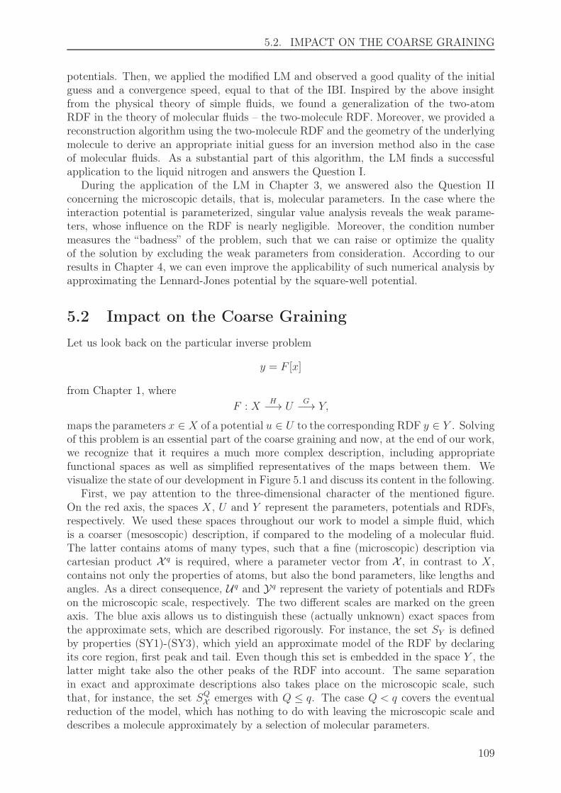
5.2. IMPACT ON THE COARSE GRAINING

potentials. Then, we applied the modified LM and observed a good quality of the initialguess and a convergence speed, equal to that of the IBI. Inspired by the above insightfrom the physical theory of simple fluids, we found a generalization of the two-atomRDF in the theory of molecular fluids – the two-molecule RDF. Moreover, we provided areconstruction algorithm using the two-molecule RDF and the geometry of the underlyingmolecule to derive an appropriate initial guess for an inversion method also in the caseof molecular fluids. As a substantial part of this algorithm, the LM finds a successfulapplication to the liquid nitrogen and answers the Question I.

During the application of the LM in Chapter 3, we answered also the Question IIconcerning the microscopic details, that is, molecular parameters. In the case where theinteraction potential is parameterized, singular value analysis reveals the weak parame-ters, whose influence on the RDF is nearly negligible. Moreover, the condition numbermeasures the “badness” of the problem, such that we can raise or optimize the qualityof the solution by excluding the weak parameters from consideration. According to ourresults in Chapter 4, we can even improve the applicability of such numerical analysis byapproximating the Lennard-Jones potential by the square-well potential.

5.2 Impact on the Coarse Graining

Let us look back on the particular inverse problem

y = F [x]

from Chapter 1, whereF : X

H−→ UG−→ Y,

maps the parameters x ∈ X of a potential u ∈ U to the corresponding RDF y ∈ Y . Solvingof this problem is an essential part of the coarse graining and now, at the end of our work,we recognize that it requires a much more complex description, including appropriatefunctional spaces as well as simplified representatives of the maps between them. Wevisualize the state of our development in Figure 5.1 and discuss its content in the following.

First, we pay attention to the three-dimensional character of the mentioned figure.On the red axis, the spaces X, U and Y represent the parameters, potentials and RDFs,respectively. We used these spaces throughout our work to model a simple fluid, whichis a coarser (mesoscopic) description, if compared to the modeling of a molecular fluid.The latter contains atoms of many types, such that a fine (microscopic) description viacartesian product X q is required, where a parameter vector from X , in contrast to X,contains not only the properties of atoms, but also the bond parameters, like lengths andangles. As a direct consequence, U q and Yq represent the variety of potentials and RDFson the microscopic scale, respectively. The two different scales are marked on the greenaxis. The blue axis allows us to distinguish these (actually unknown) exact spaces fromthe approximate sets, which are described rigorously. For instance, the set SY is definedby properties (SY1)-(SY3), which yield an approximate model of the RDF by declaringits core region, first peak and tail. Even though this set is embedded in the space Y , thelatter might take also the other peaks of the RDF into account. The same separationin exact and approximate descriptions also takes place on the microscopic scale, suchthat, for instance, the set SQX emerges with Q ≤ q. The case Q < q covers the eventualreduction of the model, which has nothing to do with leaving the microscopic scale anddescribes a molecule approximately by a selection of molecular parameters.

109


Second, we discuss closer the connections between the different spaces, which aresketched in Figure 5.2. We consider the familiar example with coarse graining of thepolystyrene in two dimensions, where the 11-atomic molecule C6H5 (with parametersfrom X q) is replaced by one spherical atom (with parameters from X). We assumethat the bonds are rigid and the single atoms interact via the Lennard-Jones potential.The resulting interaction potentials from U q and U reveal that in principle, we replace ann-polygon by a sphere, what appears as a good approximation for the present case n = 6.However, the corresponding center-of-mass RDFs from Yq and Y differ already in thefirst peak. While the molecular RDF has a double peak due to polygonal geometry of themolecule, the atomistic RDF can have only one peak due to pure Lennard-Jones inter-actions. We motivate in our work that this discrepancy should not be ignored. Similarto the simple fluid, whose interactions can be obtained via the two-atom RDF from SY ,we compute the molecular interactions via the two-molecule RDF from SQY . The latter isable to fit the double peak, and the corresponding potential from SQU reveals a penta- orhexagonal geometry of the approximate molecule (with parameters from SQX ). In otherwords, the two-molecule approximation (TMA) proposes to replace the six C-atoms bya spherical atom, but keep the five H-atoms in order to save the polygonal geometry ofthe molecule and remain on the microscopic scale. We see now that the two-atom ap-proximation (TAA) suggests a more aggressive averaging of the interactions, such thatall but mesoscopic parameters of the original molecule are lost. Since the coarse grain-ing benefits from reduced number of atoms and suffers from loss of microscopic details,it remains to decide between efficient TAA (11 7→ 1 atom(s)) and precise TMA (11 7→ 7atoms). At this place, we remind on the square-well approximation from Section 4.4.Evindently, the above analysis is much easier to do for the square-well potential than forthe Lennard-Jones potential. For a bunch of eligible mapping schemes, we can quicklydetermine how large the condition number is, how strong the single interaction param-eters are, and choose the “best” mapping scheme. Further, we can use the square-wellapproximation as a source of automatic initial guess or as a “real-time” guide during afull-blooded analysis of the dependence of the RDF on molecular parameters.

Third, we use Figure 5.1 to explain how the inversion methods of our interest work.Many actions in the figure are explicitly invertible:

(I) The mapping of the molecules to the mesoscopic atoms can be inverted by backmap-ping – reinsertion of the molecules on the given atom positions, even though it is aquite advanced procedure (see Section 1.3).

(II) Parameterization is usually bijective, such that the parameters of the given potentialcan be easily obtained by fitting (see Section 4.2.2).

(III) The two-particle approximations (TAA and TMA) provide simple maps betweenour models for RDFs and potentials, where the atomistic map is bijective (seeSection 4.2.1) and we can expect the same for the molecular one.

(IV) Truncation of the redundant peaks from the RDF leads to a subset embedded in aspace where the original RDF comes from (see Section 4.2.2).

(V) Reduction is per se not bijective, but a proper coupling of the molecular parametersallows to reconstruct the original molecule from its size partially (see Section 4.3).

However, one cannot invert the simulation in a similar explicit way – no one generates a fi-nal particle configuration from the given RDF and runs the molecular dynamics backwards

110

5.2. IMPACT ON THE COARSE GRAINING

Micro

Meso

Parameter Potential RDF

Exact

Approximate

X q

SQX

U q

SQU

Yq

SQY

X

SX

U

SU

Y

SY

Reduction

Embedding

Coupling

Reduction

Embedding

Embedding

Redundancy

Redundancy

Parameterization

Fitting

Fitting

Simulation

Simulation

TMA

TAA

MappingSch

eme

Backmapping

Averaging

CoarseGraining

Parameterization

Figure 5.1: A visualization of the relations between considered spaces.

to restore the initial configuration. The iteration function of the Iterative Boltzmann In-version (IBI) suggests that the method restores the underlying potential from U by fittingthe given center-of-mass RDF from Y . In our terms, however, the IBI makes the followingdetour

Y −→ [Y −→ SY −→ SU → U −→] ,

where the brackets denote the loop. In the coarse graining, one assumes implicitlythat Y ⊆ Y , in other words, for each center-of-mass RDF, there is a potential, such thatthe corresponding simple fluid has the same RDF. The other inclusion, Y ⊆ Y is evident,such that one regards the two spaces as identical. The modified Levenberg-Marquardtmethod avoids the scale transition arising through this identification and provides twoalternatives:

[Y −→ SY −→ SU −→ SX → X −→ U −→]

for simple fluids and[

Yq −→ SQY −→ SQU −→ SQX −→ X q −→ U q −→]

for molecular fluids. One can still use the method for coarse graining by supplying thefirst version with assumption Y = Y , what would lead to a novel, parameterized andregularized version of the IBI

Y −→ [Y −→ SY −→ SU −→ SX → X −→ U −→] .

111


Another possibility is to consider the mesoscopic potential from U as an average of themicroscopic interactions described by potentials from U q. Then, provided a proper ave-raging U q → U , one can derive an inversion method searching for microscopic poten-tials/parameters, such that the corresponding molecular RDF and the atomistic RDFcorresponding to the averaged potential fit the given molecular RDF simultaneously. Inthis fashion, the molecular parameters match the structure of the fluid on both micro-scopic and mesoscopic scales. Moreover, one computes a mesoscopic (averaged) potentialtogether with the underlying geometry of the molecule, which differs from the originalmolecule and can serve as a quality estimate and a further measure for loss of microscopicdetails.

Finally, this work proposes a new kind of the structure-based coarse graining, thatputs accent on an accurate resembling of the microscopic structure by using only theLennard-Jones potentials. Indeed, our study of a tabulated potential shows how ill-posedthe inversion is already for the simple argon fluid. As a consequence, whole regions of thepotential have nearly no impact on the structure of the fluid. That is, even if we obtaina sophisticated mesoscopic potential that resembles the given microscopic RDF, manyfeatures of the potential, for instance, a second attractive well, might play a negligiblerole in the transfer of the microscopic features to the mesoscopic scale. The accuracyof the new approach lies in a refined structure of the mesoscopic particles, which arenow non-spherical molecules consisting of atoms with intuitively clear features – size σand attractiveness ε – parameters of the Lennard-Jones (or square-well) potential. Theprice for this is a lower mapping ratio, as in the above example of polystyrene, where thestructure suggests to map eleven atoms to seven instead of one effective particle. Thiscauses a higher computational effort, but the advantage of a parameterized model foreffective interactions is evident.

5.3 Outlook

We finish this conclusion by discussing the limitations of our approach and by providinga small outlook on promising ways to circumvent them. Particularly, the two-atom RDF,which becomes to a fruit fly for our research, is only an approximation of the experi-mentally measured RDF and resembles only a part of the first peak. An approximateframework is certainly not wrong in a topic with physical background, but its capabilitiesare limited, as we saw in the study of the liquid nitrogen. At this place, the three-atomRDF opens a perspective for a more rigorous (numerical) analysis, because it is able tomodel the whole first peak of the RDF. The effort due to growing number of atoms can becancelled out by considering the square-well interactions, whose singular values resemblethat of the Lennard-Jones potential.

A possible topic for future discussion is the usage of the finite differences

F [·+∆x]− F [·]∆x

in the inversion method, where F computes the RDF or its atomistic/molecular approxi-mation. The derivative of the two-atom RDF suggests that an ad hoc strategy for choiceof the variation ∆x can lead to a noisy approximation of DF , what impairs the conver-gence behaviour of the method. Therefore, it makes sense to use the two-particle RDFs,in order to find an optimal variation. Such search is a classical problem in the numerical

112

5.3. OUTLOOK

Figure 5.2: A visualization of the elements from considered spaces.

differentiation, and the theory of inverse problems provides some fundamental solutionapproaches based on regularization [EHN-1996].

Another open problem is a further specification of the set SY ⊆ Y of molecular RDFs, asit was derived for the atomistic RDFs. On the one hand, the two-particle approximationsconfirm that the properties of the RDFs from SY ⊆ Y are meaningful and general enoughfor inclusion SY ⊆ SY . On the other hand, we saw that our inversion method using thetwo-molecule approximation cannot distinguish between simple and molecular fluid, whatleads to a loss of microscopic information (the bond length in the nitrogen molecule).In the end, it is because of the Lebesque-norm on Y , which is not able to recognize theshoulder in the first peak of the molecular RDF. However, we believe that the poor normarises from the poor description of molecular RDFs by assuming SY = SY . In order toderive further properties of the RDF, we can study the composition of the coordinationshells, because they directly affect the specific shape of the peaks in a molecular RDF.Since the underlying physics is quite general, we can analyze simple or molecular Lennard-Jones fluids in two, three and four dimensions. We emphasize that the question here isnot, whether the Lennard-Jones potential is a correct potential in other dimensions, butwhat the map G : U → Y does with the potential to compute the RDF, in dependenceof the dimension. The Monte Carlo method allows us to simulate easily molecules withrigid bonds, such that we can focus on the link between the molecular geometry and

113


the coordination shells. This approach may appear as troublesome, but, considering theredundancy in the RDF, a good description of the first coordination shell should suffice.Further, due to the good correspondence between a dense liquid and a solid, there isnot much puzzling possible, because the next-neighbour-molecules cannot be too far fromtheir positions on the crystal lattice.

In order to circumvent the direct analysis of the space Y , we can also take an establishedmathematical path. Namely, we had a similar problem with modeling the interactions viadiscretized potential in Chapter 3 and saw that a suitable parameterization H : X → U ofthe potential renders the problem well-posed. Therefore, instead of looking for a sophis-ticated definition/norm for RDFs, we can consider first a parameterization I : Z → Y ,where dim(Z) < ∞. For instance, we could follow the idea from [MGM-2005], wherethe distributions of the bond length and angles in a polymer are represented as a linearcombination of Gaussian distributions. The adaptation for our case would be to considera parameterization of the potential of mean force. It is interesting that the latter can beobtained from the molecular RDF with help of the two-atom approximation and is there-fore a potential from U . Evidently, we could not exhaust the properties of the two-particleapproximations in every sense, such that room for future work is available.

114

Appendix A

Radial Distribution Function

In this appendix, we give a comprehensive introduction to the concept of the radialdistribution function. This function has the ability to describe the structure of the givensystem of particles and can be derived from the dynamic equations of the system. However,the physical behaviour of the particles as well as the mathematical formulation of theequations depend strongly on the system size. While the system can be considered asinfinitely large in theoretical discussions, we can simulate only few thousands of particles inpractice. Therefore, we consider the theory for these two cases as a preliminary knowledgeand provide a short overview before we start with the subject.

A.1 Introduction to Statistical Physics

For the sake of simplicity, we do not consider any quantum effects, such that we canstart with the classical mechanics, as it can be found, for instance, in [LAL-1970]. Inthe mechanics, we discuss the motion (time evolution) of physical bodies. A body, whoseshape (color, size, orientation) may be neglected in the given problem setting, is called aparticle. We consider a system of N ∈ N identical particles with mass M ∈ (0,∞). Let

R :≡ (R1, . . . , RN)T , P :≡ (P1, . . . , PN)

T : [0,∞)→ RdN , 1 ≤ I ≤ N,

describe the time-dependent coordinates and momenta of the particles, respectively. Inthe Hamilton formalism, we assume that the total energy of the system can be expressedas the Hamiltonian – a function

H : RdN ×RdN → R

of the instantaneous particle coordinates R := (~R1, . . . , ~RN)T and momenta

P := (~P1, . . . , ~PN)T , which does not depend on time explicitly. The time evolution of the

system is then given by the Hamilton equations

R(t) =∂H(R(t), P )

∂P

∣∣∣∣P=P (t)

,

P (t) = − ∂H(R,P (t))

∂R

∣∣∣∣R=R(t)

. (A.1)

In principle, provided an initial state (R(0), P (0))T ∈ R2dN of the system, we can deter-mine the trajectory ((R(t), P (t))T )t≥0 ⊂ R2dN of the system. The Hamilton equations

115

APPENDIX A. RADIAL DISTRIBUTION FUNCTION

imply a conservation law – the total time derivative vanishes,

H(R(t), P (t)) =∂H(R,P (t))

∂R

∣∣∣∣R=R(t)

R(t) +∂H(R(t), P )

∂P

∣∣∣∣P=P (t)

P (t) = 0, (A.2)

that is, the total energy of the system remains constant (conserved) during the motion ofconstituent particles.

In the most popular special case, the total energy can be separated, with respect tocoordinates and momenta, in the sum

H(R,P ) = Ekin(P ) + Epot(R) (A.3)

of the kinetic energy

Ekin(P ) :=1

2M|P |2 (A.4)

and the potential energy Epot(R). Then, the Hamilton equations imply that coordinatesand momenta are coupled via

MR(t)(A.1)= M

∂H(R(t), P )

∂P

∣∣∣∣P=P (t)

(A.3)= M

∂Ekin(P )

∂P

∣∣∣∣P=P (t)

(A.4)= P (t). (A.5)

Further,

MR(t)(A.5)= P (t)

(A.1)= − ∂H(R,P (t))

∂R

∣∣∣∣R=R(t)

(A.3)= −∇Epot(R(t))

yields the Newton equations

MR(t) = F (R(t)), (A.6)

where the functionF (R) := −∇Epot(R) (A.7)

describes forces acting on the particles due to their coordinates. Now the trajectory canbe determined from the initial state (R(0), R(0))T ∈ R2dN .

In the statistical mechanics, we consider the evolution of very large systems where thenumber N of particles reaches realistic, proportional to the Avogadro number, values oforder 1023. The number of the corresponding Hamilton equations becomes overwhelming,but such a system still obeys the laws of mechanics. This allows us to derive a suitableevolution equation for the distribution of the particles, as it was done in [Español-2004].Let us denote the trajectory of the system withX(t) := (R(t), P (t))T and an instantaneousstate with X := (R,P )T . Then, we can summarize the Hamilton equations to

X(t) = L · ∇H(X(t)), (A.8)

116

A.1. INTRODUCTION TO STATISTICAL PHYSICS

where

L :=

(0 1

−1 0

)

.

If we know the initial state X(0), then formally,

X(t) =: ΓtX(0)

defines the time evolution operator Γt with natural properties

Γ0 ≡ 1, ΓtΓs ≡ Γt+s, ∀t, s,

and a kind of volume-conserving property,

| det(Γt)| = 1, ∀t. (A.9)

In a large system, we consider the evolution of the time-dependent probability densityP : R2dN×[0,∞)→ R of states. Instead of an initial state, we know a certain distributionof the initial state, given by the probability density P init : R2dN → R, such that

P(X, 0) = P init(X)

holds for all states X in an arbitrary set Ω ⊂ R2dN with |Ω| > 0. Since the evolution isdeterministic, the probabilities

P [X(0) ∈ Ω] = P [X(t) ∈ ΓtΩ]

are equal and we can write this equality in terms of the probability density,∫

Ω

P(X, 0)dX =

∫

ΓtΩ

P(X, t)dX.

Then, using the Jacobi transformation formula and (A.9), we obtain∫

Ω

P(X, 0)dX =

∫

Ω

P(ΓtX, t)dX.

Since Ω was arbitrary, the equality holds also for the integrands, especially for X = X(0),what yields the Liouville theorem

P(X(0), 0) = P(X(t), t), (A.10)

that is, the probability density remains constant along the trajectory. The total timederivative

0 =dP(X(t), t)

dt

=∂P(X(t), t)

∂t+∂P(X, t)∂X

∣∣∣∣X=X(t)

· X(t)

=∂P(X(t), t)

∂t+∂P(X, t)∂X

∣∣∣∣X=X(t)

· L · ∇H(X(t))

D=∇T

=∂P(X(t), t)

∂t+DH(X(t)) · LT · ∇P(X(t), t)

=∂P(X(t), t)

∂t−DH(X(t)) · L · ∇P(X(t), t)

117


leads to the Liouville equation

∂P(X, t)∂t

= −LP(X, t), (A.11)

where

L :≡ −DH · L · ∇ (A.12)

is the Liouville operator.Now we let the time go to infinity in order to see the state into which our large system

evolves. Considering the complexity of the interactions in such a system, we can assumethat the evolution is unstable/chaotic. That is, the system visits all possible states, suchthat any initial state/distribution appears meaningless. We say that after sufficientlylong relaxation time, the system reaches the equilibrium – there is the stationary (orequilibrium) probability density

Peq(X) := limt→∞P(X, t), ∀X ∈ R2dN . (A.13)

For any observable A = A(X), we can consider its time average

A := limΘ→∞

1

Θ

∫ Θ

0

A(X(t))dt (A.14)

or its ensemble average

〈A〉 :=∫

A(X)Peq(X)dX. (A.15)

In practice, we often assume the Ergodic hypothesis,

〈A〉 = A. (A.16)

For instance, we shall need it in Appendix B dedicated to computer simulation.The above formulation mirrors the fact that we actually consider not one system cor-

responding to a certain initial state, but a whole family (ensemble) of systems completelydetermined by a small set of dynamical invariants. The latter are the components of thevector-valued function J = J(X) with the total time derivative

J(X(t)) = 0. (A.17)

In other words, we assume that there is a function f with

Peq(X) = f(J(X)) (A.18)

and derive it in the following. Clearly, for any given value J of J at equilibrium, there isa set

Ωeq(J) := X|J(X) = Jof compatible states with the volume

Qeq(J) := |Ωeq(J)|.

118


Therefore, we can write the distribution f eq = f eq(J) of all possible values of the dy-namical invariants at equilibrium in terms of the equilibrium probability density, thatis,

f eq(J) =

∫

Peq(X)δ(J(X)− J)dX(A.18)=

∫

f(J(X))δ(J(X)− J)dX

Dirac-δ=

∫

f(J)δ(J(X)− J)dX

= f(J)Qeq(J).

Inserting this into (A.18), we obtain the probability density

Peq(X) =1

Qeq(J(X))f eq(J(X)) (A.19)

governed exclusively by the dynamical invariants.For instance, the Hamiltonian H is a dynamical invariant due to (A.2), and we can

define an ensemble of closed systems of N particles in a container of volume V withenergy E = H(X(0)), which is called the microcanonical ensemble. At equilibrium, thedistribution f eq of the energy E is time-independent and must be consistent with thegiven initial value, that is,

f eq(E) = δ(H(X)− E).Using (A.19), we can derive the microcanonical probability density

Pmc(X) =1

Qmc(E)δ(H(X)−E), (A.20)

where the volumeQmc(E) :=

∫

δ(H(X)− E)dX (A.21)

is called the microcanonical partition function.There are also other ensembles and we can derive them from the microcanonical en-

semble. Following [LL-1980], we split a large closed system in two subsystems, such thatthey can exchange the energy. We let one system, described by tuple (N, V, E), be signifi-cantly smaller than the other one, descibed by tuple (N∞, V∞, E∞). The larger system iscalled the heat bath – it will determine the evolution of the smaller subsystem by givingenergy, if the system is ′′colder′′, and by taking energy, if the system is ′′warmer′′. Thetemperature is given by

T :=1

∂S(E)∂E

, (A.22)

whereS(E) := kB ln(Qmc(E)) (A.23)

is the entropy and kB is the Boltzmann constant. If the exchange of energy stops, thatis, if

T = T∞,

the subsystems are in the thermal equilibrium with each other. Clearly, the heat bathplays the decisive role in the value of the equilibrium temperature, therefore it is also called

119


the thermostat. The ensemble governed by invariants (N, V, T ) is called the canonicalensemble. The canonical probability density and partition function are

Pc(X) =1

(2π~)dNN !Qcexp(−βH(X)), (A.24)

Qc :=1

(2π~)dNN !

∫

exp(−βH(X))dX, (A.25)

respectively, where

β :=1

kBT(A.26)

is called the inverse temperature.The function Pc is often separated into the distribution of the particle coordinates and

momenta. The first part of the distribution,

Pc(R) =

∫

Pc(R,P )dP

=

∫exp(−βH(R,P ))dP

∫exp(−βH(R,P ))dRdP

=

∫exp(−βEkin(P ))dP


· exp(−βEpot(R))∫exp(−βEpot(R))dR

=1

Zcexp(−βEpot(R)), (A.27)

plays an important role in the theory of equilibrium fluids and will be considered later inthis appendix. The normalization integral over the coordinates (configurations)

Zc :=

∫

exp(−βEpot(R))dR (A.28)

is called the configuration integral and can only be obtained in simplified circumstances.The second part of the distribution concerning the momenta,

Pc(P ) =

∫

Pc(R,P )dR

=

∫exp(−βH(R,P ))dR

∫exp(−βH(R,P ))dRdP

=

∫exp(−βEpot(R))dR

∫exp(−βEpot(R))dR

· exp(−βEkin(P ))∫exp(−βEkin(P ))dP

=1


exp(−βEkin(P )). (A.29)

is the Maxwell-Boltzmann velocity distribution. Its normalization integral can be obtainedexplicitly

∫

exp(−βEkin(P ))dP =

(∫ ∞

−∞exp

(

−βp2

2M

)

dp

)dN

=

(√

2M

β

∫ ∞

−∞exp

(−q2

)dq

)dN

=

(2πM

β

)dN/2

=

(2π~

Λ

)dN

, (A.30)

120


where

Λ :=

√

2πβ~2

M(A.31)

is the de Broglie thermal wavelength and ~ is the Planck constant.We emphasize that different ensembles are just different descriptions of systems in the

equilibrium. For example, in the thermal equilibrium, the total energy is conserved (noexchange) and the microcanonical ensemble can be used to describe the subsystems. Wedefined the temperature by considering the special splitting of a large closed system, butit is also defined for all other ensembles. Additionally, we can consider the exchange ofvolume and particles between subsystems, in order to define the pressure

P := −∂E(V )

∂V(A.32)

and the chemical potential

µ :=∂E(N)

∂N. (A.33)

The ensemble governed by invariants (µ, V, T ) is called the grand canonical ensemble.One can show that the probability density of dynamical states in the grand canonicalensemble is

Pgc(X ;N) =1

(2π~)dNN !Qgcexp(−β(H(X)− µN)), (A.34)

where

Qgc :=

∞∑

N=0

eβµN

(2π~)dNN !

∫

exp(−βH(X))dX (A.35)

is the grand canonical partition function. It is convenient to introduce the activity

a :=eβµ

Λd, (A.36)

and use the (intuitively clear) relation to the canonical probability density,

Pgc(X; N) = P[

N = N]

· Pc(X)|N=N , (A.37)

where

P[

N = N]

=

∫

Pgc(X; N)dX

=1

(2π~)dNN !Qgc

∫

exp(−β(H(X)− µN))dX

=eβµN

(2π~)dNN !Qgc

∫

exp(−βH(X))|N=N dX

=eβµN

(2π~)dNN !Qgc

(2π~

Λ

)dN

Zc|N=N

=aN

N !QgcZc|N=N (A.38)

121


is the probability that the system contains precisely N particles. A similar relation canbe derived for the partition functions,

Qgc =

∞∑

N=0

aN

N !Zc. (A.39)

In the statistical thermodynamics, we leave the probability densities and describe dif-ferent ensembles exclusively through the dynamical invariants, which are called in thenew context the thermodynamic quantities. It is usual to separate the quantities in theextensive (additive), like

N = N1 +N2,

V = V1 + V2,

E = E1 + E2,

S = S1 + S2,

and intensive (non-additive), like

T = T1 = T2,

P = P1 = P2,

µ = µ1 = µ2.

Further, the extensive quantities N, V, S are seen as conjugated to the intensive quantitiesµ, P, T , respectively. The corner stones of the thermodynamics are the thermodynamicpotentials – functions, which allow to derive the quantities from their conjugated coun-terparts. For instance,

F := E − TS = −kBT lnQc, (A.40)

Φ := F − µN = −PV = −kBT lnQgc (A.41)

are the thermodynamic potentials of the canonical and grand canonical ensembles, respec-tively. Conveniently, the entropy S(E) can be also seen as the thermodynamic potentialof the microcanonical ensemble (see (A.23)), but often, the energy E(S) is preferred. Anythermodynamic quantity can be obtained from the total differentials

dE = TdS − PdV + µdN, (A.42)

dF = −SdT − PdV + µdN, (A.43)

dΦ = −SdT − PdV −Ndµ. (A.44)

Equation (A.42) is often referred to as the first law of thermodynamics. One of the mostimportant tasks of thermodynamics is to find the equation of state for the given system,that is, an equation of the form

f(T, P, ρ) = 0,

coupling the temperature T , pressure P and the (number) density

ρ :=N

V. (A.45)

122

A.2. DEFINITION OF THE RDF FOR A SIMPLE FLUID

Example “Ideal Gas”:Ideal gas is the system of particles without interactions, that is, where the potentialenergy Epot ≡ 0 and from the mechanical point of view, only the momenta of particlescan be considered. From the thermodynamic viewpoint, due to missing interactions, manyintegrals become trivially obtainable, for instance,

Zc = V N ,

Qc =V N

ΛdNN !,

Qgc =∞∑

N=0

aN

N !V N = eaV ,

F = −kBT ln

(V N

ΛdNN !

)

Stirling≈ −kBT (N lnV − dN ln Λ−N lnN +N),

Φ = −kBT ln eaV = −kBTaV.

Then, the first law of thermodynamics yields the equation of state for the ideal gas,

P(A.43)= − ∂F

∂V

∣∣∣∣N,T≡const

= ρkBT. (A.46)

Even more, we have

P(A.41)= − 1

VΦ = akBT

and by comparing to (A.46), we state that the ideal gas activity a = ρ.

We can see in the above example that, disregarding the different abstraction levels,the classical dynamics and the statistical thermodynamics do not loose the link to eachother. Using this link, one can show a more exact equation of state,

P = ρkBT −1

V d

⟨N∑

I=1

~RI · ~∇IEpot(R)

⟩

, (A.47)

known as the virial equation. Setting Epot ≡ 0, we see that it is consistent with ourexample.

A.2 Definition of the RDF for a Simple Fluid

Now, when we understand the dynamics of a large system towards the equilibrium state,we can start with the subject of this appendix. We want to describe the structure ofliquids and gases, which are systems of many moving particles. Liquid, gas and solid arethe three classical states of matter (phases). Liquid and gas are also called fluid for theirability to flow and take the shape of a container. However, while a gas tries to fill thewhole container at cost of the density, a liquid keeps its density nearly constant. Thedensities of both a liquid and a solid are of the same order and much higher than in agas. Since the particles of a solid do not move almost (|Ekin| ≪ |Epot|), we consider onlyfluid phase in the following. For the sake of simplicity, we restrict our consideration tothe simple fluids, where the particles are spherical.

123


Following [HM-2006], we model a simple fluid as a large system of N ∈ N identicalparticles with mass M ∈ (0,∞) and the Hamiltonian of the form (A.3), so that we canforget their momenta and just work with their coordinates R ∈ RdN and the potentialenergy. The latter is nothing else than N -body interaction potential, thus we approximateit via the sum

Epot(R) :=1

2

N∑

I=1

N∑

J 6=IU (2)(~RI , ~RJ) (A.48)

of the pair interactions given by potentials U (2) : Rd × Rd → R. In the following, weassume that the interaction potential is translationally invariant, that is,

U (2)( ~X, ~Y ) = U (2)( ~X + ~Z, ~Y + ~Z), ∀~Z ∈ Rd, (A.49)

and rotationally invariant, that is,

U (2)( ~X, ~Y ) = U (2)(A ~X,A~Y ), ∀A ∈ SO(d). (A.50)

In this case, we obtain

U (2)( ~X, ~Y )(A.49)= U (2)(0, ~Y − ~X)

(A.50)= U (2)(0, |~Y − ~X|~e1),

that is, viaU(r) := U (2)(0, r~e1), (A.51)

we define a radial potential U : (0,∞)→ R with

U (2)( ~X, ~Y ) = U(| ~X − ~Y |), ∀ ~X, ~Y ∈ Rd.

The physics has a collection of common interaction potentials, but not all of them areproper for modeling of the liquid state. Such potential U must at least reflect the Pauliexclusion principle, that is,

limr→0

U(r) =∞,

and vanish, if two particles are too far from each other, that is,

limr→∞

U(r) = 0.

For example, the hard-sphere potential

UHS(r) :=

∞, 0 < r < σ,0, σ ≤ r,

(A.52)

is often used for fluid phase simulations. The parameter σ > 0 represents the size of theparticles, such that two particles cannot be closer than their sizes allow. However, fluid isquite not a liquid, until the potential has an attractive part keeping the particles togetherand forming a stable liquid phase. In contrast, the square-well potential

USW(r) :=

∞, 0 < r < σ,−ε, σ ≤ r < γσ,0, γσ ≤ r,

(A.53)

124


0 5 10 15 20 25 300

0.5

1

1.5

2

2.5

3

3.5

distance [A]

Figure A.1: A radial distribution function of liquid argon, obtained in a neutron scatteringexperiment [YKWK-1973].

has an attractive well with depth ε > 0 and width σ(γ − 1) > 0. Another appropriatechoice for liquid simulations is the hard-core Yukawa potential

UY(r) :=

∞, 0 < r < σ,

−εσrexp

(−λ(rσ− 1)), σ ≤ r,

(A.54)

with λ > 0. Due to quantum-mechanical reasons, the leading term in the series expansionof the attractive interaction between neutral particles is of order O(r−6) for large r, whatsuggests the Buckingham potential

UB(r) := Ae−Br − C

r6(A.55)

and the famous Lennard-Jones potential

ULJ(r) := 4ε

((σ

r

)12

−(σ

r

)6)

. (A.56)

We notice that all potentials are piecewise smooth, real-valued functions on (0,∞) withnegative, but finite minimal values.

Even though the interaction potential allows us to derive the equations of motion for theparticles, we are not interested in the exact dynamics and rather look at the system fromthe statistical viewpoint. We assume the fluid to be at equilibrium, where the dynamicalstates obey a certain probability density Peq. Similar to the interaction potential, whichspecifies the energy for the given particle coordinates and takes a radially symmetric form

125


in our model, the distribution can posess some symmetries, which allow us to reduce thedistribution to a function, which is translationally and rotationally invariant. The latteris called the radial distribution function (RDF). This function describes the distributionof the distance between pairs of particles and can be determined experimentally for aconcrete matter by neutron or x-ray scattering (see Figure A.1).

In order to give an explicit definition of the RDF, we have to choose one of the ensemblesfrom the framework of statistical mechanics. Therefore, the “definitions” may be also readas derivations. We present the definition of the RDF in the grand canonical ensemble (orµV T -ensemble, after governing invariants), where

I) the chemical potential µ is constant,

II) the fluid is contained in a region Ω ⊆ Rd of constant volume V , e.g.

~RI1≤I≤N ⊂ Ω :=

[

−L2,L

2

]d

, V = Ld, L > 0,

III) the temperature T is constant,

and in the canonical ensemble (or NV T -ensemble), where

I) the particle number N is constant

and the properties II) and III) are inherited from the grand canonical ensemble. Clearly,different ensembles provide different models (expressions), but in the thermodynamiclimit, that is, when N → ∞ and V → ∞ with the constant density ρ, the two descrip-tions become identical and agree with experimental data. We note that V → ∞ leadsto L → ∞ and Ω → Rd, that is, Ω becomes translationally and rotationally invariant.However, the infinity is unreachable in practice, so that the experimental RDF is given ona finite interval – we can see this in Figure A.1, where the interparticle distances hardlyreach 30 [Å]. Thus, in our theoretical considerations, we often work with finite N and V ,mostly assuming them large enough and occasionally infinite. Further, we shall switch be-tween the ensembles in order to use their specific advantages. For these reasons, we provethe following theorems not in the mathematically rigorous manner, but in the frameworkof the convenient calculus that is often used in the physical literature for argumentation.

The simplest derivation of the RDF can be made in the canonical ensemble. Fromthe statistical mechanics, we know the equilibrium probability density Pc as a function ofparticle coordinates R ∈ RdN . The function contains redundant information – since theparticles of considered fluid are identical, we can interchange any I-th particle and anyJ-th particle, that is,

Pc(~R1, . . . , ~RI , . . . , ~RJ , . . . , ~RN) = Pc(~R1, . . . , ~RJ , . . . , ~RI , . . . , ~RN ). (A.57)

Further, we are not always interested in all details of the distribution, therefore we de-fine simplified probability densities, where the unnecessary information is removed byintegration. For each 1 ≤ n ≤ N , the (reduced) n-particle density is

ρ(n)(~R1, . . . , ~Rn) :=N !

(N − n)!

∫

Pc(R)d~Rn+1 . . . d ~RN (A.58)

and the n-particle distribution function is

g(n)(~R1, . . . , ~Rn) :=ρ(n)(~R1, . . . , ~Rn)

ρ(1)(~R1) . . . ρ(1)(~Rn). (A.59)

126


The following results deal with the properties of the reduced distributions, which describethe properties of the fluid. In this regard, we remind on our assumption that the inter-action potential U as well as the region Ω are translationally and rotationally invariant.However, it can still happen that under these symmetric conditions, the symmetry brea-king takes place, that is, configurations of the particles and related properties of the fluidare not symmetric. For instance, at the liquid-solid phase transition, the particles of thesystem form a lattice, which preserves partially the translational symmetry, while therotational symmetry is completely out. Therefore, we assume in the following that nosuch phenomenon occurs.

Theorem P1:The n-particle density is translationally and rotationally invariant.Proof: Any rotation and any translation in Rd can be described as the transformation

Φ : Rd → Rd,~X 7→ A ~X + ~Z (A.60)

with A ∈ SO(d) and ~Z ∈ Rd. Then,

Epot(Φ(~R1), . . . ,Φ(~RN))(A.48)=

1

2

N∑

i=1

N∑

j 6=iU(|Φ(~Ri)− Φ(~Rj)|)

(A.60)=

1

2

N∑

i=1

N∑

j 6=iU(|A~Ri + ~Z −A~Rj − ~Z|)

A∈SO(d)=

1

2

N∑

i=1

N∑

j 6=iU(|~Ri − ~Rj |)

(A.48)= Epot(R), (A.61)

that is, the potential energy is translationally and rotationally invariant. Similarly,

ρ(n)(~R1, . . . , ~Rn)(A.58)=

1

Zc

N !

(N − n)!

∫

exp(−βEpot(R)

)d~Rn+1 . . . d ~RN

(A.61)=

1

Zc

N !

(N − n)!

∫

exp(

−βEpot(Φ(~R1), . . . ,Φ(~RN )))

d~Rn+1 . . . d ~RN

Substitution(s):~Si := Φ(~Ri),

d~Si = d~Ri, n+ 1 ≤ i ≤ N

JTF=

1

Zc

N !

(N − n)!·∫

exp(

−βEpot(Φ(~R1), . . . ,Φ(~Rn), ~Sn+1, . . . , ~SN))

·d~Sn+1 . . . d~SN(A.58)= ρ(n)(Φ(~R1), . . . ,Φ(~Rn)).

127


Corollary:For all ~R ∈ Rd, we have

ρ(1)(~R) =N

V= ρ, (A.62)

that is, the one-particle density is just the density of the fluid.Proof:

ρ(1)(~R)P1= ρ(1)(0)

=1

V

∫

Ω

ρ(1)(0)d~R1

P1=

1

V

∫

Ω

ρ(1)(~R1)d~R1

(A.58)=

1

V

∫

Ω

(

N

∫

Pc(R)d~R2 . . . d ~RN

)

d~R1

(A.27)=

N

V= ρ.

Theorem P2:ρ(n) is a function of n(n−1)

2scalar arguments.

Proof: Per definition, ρ(n) is a function of n vectors ~R1, . . . , ~Rn, where the latter can befreely rotated and shifted in space, without changing the value of the function (accordingto Theorem P1). We take these n vectors as vertices of an (n−1)-simplex. This geometricfigure is fully determined by the lengths of its edges |~RJ− ~RI |, 1 ≤ I ≤ n, I+1 ≤ J ≤ n.

According to Theorem P1, we have

ρ(2)(~R1, ~R2) = ρ(2)(0, |~R1 − ~R2|~e(1)), ∀~R1, ~R2 ∈ Rd. (A.63)

Further, Theorem P2 implies directly that the pair distribution function

g(2)(A.62)≡ 1

ρ2ρ(2)

depends on only one scalar argument. In other words, there is the radial distributionfunction (RDF) g : (0,∞)→ R with

g(2)(~R1, ~R2) = g(|~R1 − ~R2|), ∀~R1, ~R2 ∈ Rd.

Respective (A.63), the RDF is given by

g(r) := g(2)(0, r~e(1)). (A.64)

We caution that this definition only makes sense under the above assumption of symmetry.The definition of the RDF in the grand canonical ensemble can be obtained in the

similar way. While in the canonical ensemble, the number of particles is an implicitparameter of all distributions and quantities, in the grand canonical ensemble, where thechemical potential µ and not N is constant, the number of particles is an explicit variable

128

A.3. GENERAL PROPERTIES OF THE RDF

of the distribution. Relation (A.37) between the two ensembles suggests to define the(reduced) n-particle density for each 1 ≤ n ≤ N via

ρgc,(n)(~R1, . . . , ~Rn) :=

∞∑

N=n

P[

N = N]

· ρ(n)(~R1, . . . , ~Rn)∣∣∣N=N

. (A.65)

Then, we can adopt the expressions (A.59) for the n-particle distribution function and(A.64) for the RDF.

Example “Ideal Gas”:Since the potential energy Epot ≡ 0, we obtain

Zc =

∫

exp(−βEpot(R))dR = V N ,

P c(R) =1

Zcexp(−βEpot(R)) =

1

V N,

ρ(2)(~R1, ~R1) = N(N − 1)

∫

P c(R)d~R3 . . . d ~RN

=N(N − 1)V N−2

V N=N(N − 1)

V 2,

g(r) =1

ρ2ρ(2)(0, r~e(1)) = 1− 1

N.

that is, in the thermodynamic limit,

g(r) = 1 (A.66)

for the ideal gas.

A.3 General Properties of the RDF

The two ensembles provide us a powerful calculus, which can be applied to derive somegeneral properties of the RDF. Due to equivalence of the two descriptions, we can switchbetween the ensembles, in order to use their specific advantages for the particular deriva-tion.

Theorem P3:We can write the pair distribution function g(2) and the RDF in terms of ensemble averagesof Dirac δ-functions,

g(2)( ~X, ~Y ) =1

ρ2

N∑

I=1

N∑

J 6=I

⟨

δ( ~X − ~RI)δ(~Y − ~RJ)

⟩

, (A.67)

g(r) =V

N2

N∑

I=1

N∑

J 6=I

⟨

δ(r~e(1) − ~RJ + ~RI)

⟩

. (A.68)

129


Proof:

g(2)( ~X, ~Y )(A.59)=

ρ(2)( ~X, ~Y )

ρ(1)( ~X)ρ(1)(~Y )

(A.62)=

1

ρ2ρ(2)( ~X, ~Y )

(A.58)=

1

ρ2N(N − 1)

∫

Pc( ~X, ~Y , ~R3, . . . , ~RN)d~R3 . . . d ~RN

Dirac-δ=

1

ρ2N(N − 1)

∫

δ( ~X − ~R1)δ(~Y − ~R2)Pc(R)dR

(A.57)=

1

ρ2

N∑

I=1

N∑

J 6=I

∫

δ( ~X − ~RI)δ(~Y − ~RJ)Pc(R)dR

(A.15)=

1

ρ2

N∑

I=1

N∑

J 6=I

⟨

δ( ~X − ~RI)δ(~Y − ~RJ)

⟩

,

g(r)(A.64)= g(2)(0, r~e(1))

P1=

1

V

∫

g(2)( ~W, r~e(1) + ~W )d ~W

(A.67)=

1

V

∫1

ρ2

N∑

I=1

N∑

J 6=I

⟨

δ( ~W − ~RI)δ(r~e(1) + ~W − ~RJ)

⟩

d ~W

Dirac-δ=

V

N2

N∑

I=1

N∑

J 6=I

⟨

δ(r~e(1) − ~RJ + ~RI)

⟩

.

The above theorem shows that g(r) tests for each particle pair, if they are at distance rin average. Further, the next theorem reveals that the RDF also counts the particles dur-ing testing.

Theorem P4:

ρ

∫

g(r)|∂B(r)|dr = N − 1.

Proof:∫

g(r)|∂B(r)|dr =N(N − 1)

ρ2

∫

Pc(0, r~e1, ~R3, . . . , ~RN)|∂B(r)|drd~R3 . . . d ~RN

JTF=

N(N − 1)

ρ2

∫

Pc(0, ~R2, . . . , ~RN)d~R2 . . . d ~RN

JTF=

N(N − 1)

V ρ2

∫

Pc(~R1, . . . , ~RN)d~R1 . . . d ~RN

(A.27)=

N − 1

ρ.

Further, we can obtain the pressure P and the potential energy Epot from the givenRDF.

130


Theorem P5:

P = ρkBT −ρ2

2d

∫ ∞

0

DU(r)g(r)|∂B(r)|rdr, (A.69)

⟨Epot

⟩=

N2

2V

∫ ∞

0

U(r)g(r)|∂B(r)|dr. (A.70)

Proof: We use the virial equation to write the pressure P in the form

P(A.47)= ρkBT −

1

V d

⟨

1

2

N∑

I=1

N∑

J 6=IDU(|~RIJ |)|~RIJ |

⟩

(A.15)= ρkBT −

1

2V d

N∑

I=1

N∑

J 6=I

∫

DU(|~RIJ |)|~RIJ |Pc(R)dR

(A.57)= ρkBT −

N(N − 1)

2V d

∫

DU(|~R21|)|~R21|Pc(R)dR

(A.59)= ρkBT −

N(N − 1)

2V d

ρ2

N(N − 1)

∫

DU(|~R21|)|~R21|g(2)(~R1, ~R2)d~R1d~R2

P1= ρkBT −

ρ2

2V d

∫

DU(|~R21|)|~R21|g(2)(0, |~R21|~e1)d~R1d~R2

JTF= ρkBT −

ρ2

2d

∫

DU(|~R|)|~R|g(2)(0, |~R|~e1)d~R

JTF= ρkBT −

ρ2

2d

∫ ∞

0

DU(r)g(r)|∂B(r)|rdr.

Similarly, we obtain

⟨Epot

⟩ (A.48)=

⟨

1

2

N∑

I=1

N∑

J 6=IU(|~RIJ |)

⟩

(A.15)=

1

2

N∑

I=1

N∑

J 6=I

∫

U(|~RIJ |)Pc(R)dR

(A.57)=

N(N − 1)

2

∫

U(|~R21|)Pc(R)dR

=N(N − 1)

2

∫

U(|~R21|)(∫

Pc(R)d~R3 . . . d ~RN

)

d~R1d~R2

(A.59)=

N(N − 1)

2

ρ2

N(N − 1)

∫

U(|~R21|)g(2)(~R1, ~R2)d~R1d~R2

P1=

ρ2

2

∫

U(|~R21|)g(2)(0, |~R21|~e1)d~R1d~R2

JTF=

ρ2V

2

∫

U(|~R|)g(2)(0, |~R|~e1)d~R

JTF=

N2

2V

∫ ∞

0

U(r)g(r)|∂B(r)|dr.

In a similar way, we can derive another important relation between the RDF and theunderlying interaction potential.

131


Theorem P6:The RDF can be written as a rescaled ensemble average of the function

S(r;R) :=1

2

N∑

I=1

N∑

J 6=Iδ(r − |~RIJ |),

more precisely,

〈S(r;R)〉 = 2πr2N2

Vg(r).

The advantage of this respresentation is that we can determine the functional derivativeof the latter average with respect to the potential U , that is,

∂〈S(r;R)〉∂U(s)

= −β(〈S(r;R)S(s;R)〉 − 〈S(r;R)〉〈S(s;R)〉). (A.71)

Proof: Evidently, the function S(r;R) is nothing else than the instantaneous systemconfiguration in terms of Dirac δ-functions. Indeed, similar to Theorem P5, we can writethe instantaneous potential energy via

Epot(R)(A.48)=

1

2

N∑

I=1

N∑

J 6=IU(|~RIJ |)

Dirac-δ=

1

2

N∑

I=1

N∑

J 6=I

∫ ∞

0

U(r)δ(r − |~RIJ |)dr

=

∫ ∞

0

U(r)S(r;R)dr.

Moreover, the ensemble average over the instantaneous configurations yields a rescaledRDF, more precisely,

〈S(r;R)〉 =1

2

N∑

I=1

N∑

J 6=I

⟨

δ(r − |~RIJ |)⟩

(A.15)=

1

2

N∑

I=1

N∑

J 6=I

∫

δ(r − |~RIJ |)Pc(R)dR

(A.57)=

N(N − 1)

2

∫

δ(r − |~R21|)Pc(R)dR

JTF=

V N(N − 1)

2

∫

δ(r − |~R2|)Pc(0, ~R2, . . . , d ~RN)d~R2 . . . d ~RN

JTF=

V N(N − 1)

2

∫

δ(r − s)4πs2Pc(0, s~e1, ~R3, . . . , d ~RN)dsd~R3 . . . d ~RN

Dirac-δ=

4πr2V N(N − 1)

2

∫

Pc(0, r~e1, ~R3, . . . , d ~RN)d~R3 . . . d ~RN

=4πr2V N(N − 1)

2

ρ2

N(N − 1)g(r)

=2πr2N2

Vg(r).

132


Then, the derivative of the ensemble average is given by

∂〈S(r;R)〉∂U(s)

=∂

∂U(s)

∫

S(r;R)Pc(R)dR

=∂

∂U(s)

(∫S(r;R) exp(−βEpot(R))dR

Zc

)

=∂

∂U(s)

(∫S(r;R) exp

(−β∫∞0U(r)S(r;R)dr

)dR

∫exp

(−β∫∞0U(r)S(r;R)dr

)dR

)

= −β(〈S(r;R)S(s;R)〉 − 〈S(r;R)〉〈S(s;R)〉).

The above results are obtained in the simple formalism of the canonical ensemble andprovide nice tools for computer simulation of the fluid or for analysis of experimentaldata. However, using the rather complicated model of the grand canonical ensemble, wecan derive even more powerful statement.

Theorem P7:If we assume, that the activity a = ρ for ρ→ 0, then

limρ→0

ggc,(n)(~R1, . . . , ~Rn) = exp(−βEpot(~R1, . . . , ~Rn)).

Proof: We write the distribution function as the series

ggc,(n)(~R1, . . . , ~Rn)P1=

1

ρnρgc,(n)(~R1, . . . , ~Rn)

(A.65)=

1

ρn

∞∑

N=n

P[

N = N]

· ρ(n)(~R1, . . . , ~Rn)∣∣∣N=N

(A.38)=

1

ρn

∞∑

N=n

aN

N !QgcZc|N=N ρ(n)(~R1, . . . , ~Rn)

∣∣∣N=N

(A.58)=

1

ρn

∞∑

N=n

aN

N !QgcZc|N=N

· N !

(N − n)! Zc|N=N

∫

exp(−βEpot(~R1, . . . , ~RN ))d~Rn+1 . . . d ~RN

(A.58)=

1

ρn1

Qgc

∞∑

N=n

aN

(N − n)!

∫

exp(−βEpot(~R1, . . . , ~RN))d~Rn+1 . . . d ~RN .

Under the assumption a = ρ, the density disappears from the first term of the series.That is, if we let the density ρ go to zero, the remaining terms vanish. Similarly, forρ→ 0, only the first term of the series

Qgc (A.39)=

∞∑

N=0

aN

N !Zc

(A.28)=

∞∑

N=0

aN

N !

∫

exp(−βEpot(~R1, . . . , ~RN))d~R1 . . . d ~RN

remains and equals 1, because the potential energy of an empty system is zero.

133


We remark that a = ρ for the ideal gas, as we have shown in Section A.1. In the case,where the density goes to zero, the interactions between particles are very rare, so thatthe system behaves nearly like the ideal gas and the assumption of Theorem P7 can beconsidered as given. The direct consequence of the above theorem is the equation

limρ→0

g(r) = limρ→0

g(2)(0, r~e(1))

= exp(−βEpot(0, r~e(1)))

= exp(−βU(r)), (A.72)

called the low-density limit of the RDF.

A.4 Special Case of the Lennard-Jones Potential

While the previous results are valid for the general interaction potential and show howmuch information can be retrieved from the RDF, we also test a special case of theLennard-Jones potential (A.56), in order to obtain a deeper insight into the nature of thedistribution. To do so, we use the formalism of the canonical ensemble and assume thatour system has a large, but finite size

L =d√V = d

√

N

ρ.

We consider the RDF

g(r) =N(N − 1)

ρ2

∫

Pc(0, r~e1, ~R3, . . . , ~RN)d~R3 . . . d ~RN , r ∈[

0,L

2

]

,

as a function of the distance, parameterized with T , L and the parameters ε, σ of theLennard-Jones potential

U(r; ε, σ) = 4ε

((σ

r

)12

−(σ

r

)6)

.

The following properties of the potential attract our attention:

U(r; aε, σ) = 4aε

((σ

r

)12

−(σ

r

)6)

= aU(r; ε, σ),

U(r; ε, bσ) = 4ε

((bσ

r

)12

−(bσ

r

)6)

= U(r

b; ε, σ

)

.

Then, the potential energy takes the form

Epot(R; ε, σ) =1

2

N∑

I=1

N∑

J 6=IU(|~RI − ~RJ |; ε, σ)

134

A.4. SPECIAL CASE OF THE LENNARD-JONES POTENTIAL

and satisfies the relations

Epot(R; aε, σ) = aEpot(R; ε, σ), (A.73)

Epot(R; ε, bσ) = Epot

(1

bR; ε, σ

)

. (A.74)

This motivates us to rewrite the RDF of the Lennard-Jones fluid in the parameterizedform,

g(s;T, L, ε, σ) =N(N − 1)

ρ2

∫

ΩN−2

Pc(0, Ls~e1, ~R3, . . . , ~RN ;T, L, ε, σ)d~R3 . . . d ~RN

=(N − 1)L2d

N

∫

ΩN−2

Pc(0, Ls~e1, ~R3, . . . , ~RN ;T, L, ε, σ)d~R3 . . . d ~RN

JTF=

(N − 1)LNd

N

∫

ΩN−2/L

Pc(0, Ls~e1, L~S3, . . . , L~SN ;T, L, ε, σ)d~S3 . . . d~SN

for all s ∈[0, 1

2

].

Theorem P8:The RDF of the Lennard-Jones fluid (as a function of s) depends on only two parame-ters – the first one is either T or ε, the second one is either L or σ.Proof: Let us also parameterize the probability density of the canonical ensemble and theconfiguration integral,

Pc(R;T, L, ε, σ) =1

Zc(T, L, ε, σ)exp(−βEpot(R; ε, σ)),

Zc(T, L, ε, σ) =

∫

ΩN

exp(−βEpot(R; ε, σ))dR

JTF= LNd

∫

ΩN/L

exp(−βEpot(LS; ε, σ))dS. (A.75)

Then, we see that

Zc(T, L, aε, bσ)(A.75)= LNd

∫

ΩN/L

exp(−βEpot(LS; aε, bσ))dS

(A.73),(A.74)= LNd

∫

ΩN/L

exp

(

−aβEpot

(L

bS; ε, σ

))

dS

= bNd(L

b

)Nd ∫

ΩN/L

exp

(

−aβEpot

(L

bS; ε, σ

))

dS

(A.75)= bNdZc

(T

a,L

b, ε, σ

)

(A.76)

135


and

g(s;T, L, aε, bσ) =(N − 1)LNd

NZc(T, L, aε, bσ)

·∫

Ω(N−2)/L

exp(−βEpot(0, Ls, LS3, . . . , LSN ; aε, bσ))

·dS3 . . . dSN

(A.76)=

(N − 1)(Lb

)Nd

NZc(Ta, Lb, ε, σ

)

·∫

Ω(N−2)/L

exp(−βEpot(0, Ls, LS3, . . . , LSN ; aε, bσ))

·dS3 . . . dSN

(A.73),(A.74)=

(N − 1)(Lb

)Nd

NZc(Ta, Lb, ε, σ

)

·∫

Ω(N−2)/L

exp

(

−aβEpot

(

0,L

bs,L

bS3, . . . ,

L

bSN ; ε, σ

))

·dS3 . . . dSN

= g

(

s;T

a,L

b, ε, σ

)

for all s ∈[0, 1

2

]. In particular,

g(s;T, L, ε, σ) = g

(

s;T

ε,L

σ, 1, 1

)

,

g(s;T, L, ε, σ) = g(

s; 1, 1,ε

T,σ

L

)

.

A.5 Definition of the RDF for a Molecular Fluid

The definition of the RDF can be extended also to the case of the molecular fluid whoseparticles are identical but should not be considered as spherical, for example, the rod-shaped molecules of nitrogen N2 and carbon dioxide CO2, or the bended molecule of waterH2O. In this case, we have to model also the bonded interactions inside the molecules, forinstance, by potentials of the form

vbondi (ℓ) =

1

2kbondi (ℓ− ℓi)2,

vbendi (θ) =

1

2kbendi (θ − θi)2,

vtorsi (φ) =

1

2ktorsi (φ− φi)2.

In other words, we model a molecule as a composition of diverse spherical particles ar-ranged by constants

ℓi : 1 ≤ i ≤ Nbond ⊂ R,

θi : 1 ≤ i ≤ Nbend ⊂ R,

φi : 1 ≤ i ≤ N tors ⊂ R,

136

A.5. DEFINITION OF THE RDF FOR A MOLECULAR FLUID

called bond lengths, bending angles and torsion angles, respectively. We call the con-stituent particles atoms and label them with numbers 1, . . . , Natom. The followingtheory is not affected by the chosen labeling, because we shall work with the maps

τ : 1, . . . , Natom → 1, . . . , N type,ν : 1, . . . , Natom → 1, . . . , N,

assigning the given atom label to one of N type types and one of N molecules. For example,two water molecules would be represented by

Label i Type τ(i) Atom Molecule ν(i)1 1 H 12 2 O 13 1 H 14 1 H 25 2 O 26 1 H 2

Surely, similar to the simple fluid, we could also describe the system through the atomcoordinates

~ri : 1 ≤ i ≤ Natom ⊂ Rd,

masses (ma)Ntype

a=1 and the interaction potential

u(2)a,b : R

d ×Rd → R

for each pair of atoms of a-th and b-th types, 1 ≤ a, b ≤ N type. However, this descriptionwould contain many redundant degrees of freedom – the shape of the molecules can beoften considered as rigid, that is, the changes of the shape due to the bonded interactionsare negligible, when averaged over all molecules of the fluid. On the other hand, the bondlengths, bending angles and torsion angles would not suffice for a good description – theydo not specify the “positions” of the molecules. The latter, following [GG-1984], can bedefined by the coordinates of molecular centers of mass

~RI :=1

M

∑

i:ν(i)=I

mτ(i)~ri ∈ Rd, 1 ≤ I ≤ N,

and by the molecular orientations

WI ∈ Q ⊂ Rq, 1 ≤ I ≤ N,

whereM :=

∑

i:ν(i)=1

mτ(i)

is the total mass of the first molecule (molecules are identical). It is easily seen that for asuitable Q ⊂ Rq, the set of variables allows to determine the positions ~ri of the atoms.In d = 3 dimensions, the orientation of a rigid body (molecule) is given by Euler angles

(ψ, ϕ, γ) ∈ (0, π)× (−π, π)× (0, 2π),

137


that is, Q ≃ S2 × S1 and |Q| = 8π2. If the molecule has symmetries, the degrees offreedom reduce – for a rod-shaped molecule, the spherical coordinates

(ψ, ϕ) ∈ (0, π)× (−π, π)

will suffice, that is, Q ≃ S2 and |Q| = 4π. Finally, the potential energy for a pair ofmolecules is the sum of potential energies between building atoms, so that we can definethe molecular pair interaction potential as

U (2) : Rd ×Rd ×Rq ×Rq → R,

(~RI , ~RJ ,WI ,WJ) 7→∑

i:ν(i)=I

∑

j:ν(j)=J

u(2)τ(i),τ(j)(~ri, ~rj).

Summarizing the above definitions in other words, we just carried out a scale transi-tion. We could model the molecular fluid on the microscopic scale – we would cope withthe bonded interactions vbond

i , vbendi , vtors

i and non-bonded interactions u(2)a,b of single atoms(microscopic particles) ~ri with masses ma. But in this case, we could not assumetranslationally and rotationally invariant interactions in the sense of definitions (A.49)and (A.50), which hold on the microscopic scale and implicitly require a single potentialfor all interactions. We remind that the concept of the RDF holds only under this as-sumption. Therefore, we prefer to consider the molecular fluid on a mesoscopic scale, asa family of N ∈ N identical molecules (mesoscopic particles) (~RI ,WI) with mass Mand interaction potential U (2). Indeed, a non-spherical molecule, “averaged” over all ori-entations, has a nearly spherical shape. For fixed molecular orientations WI, we obtainthe relations

U (2)(~RI , ~RJ ,WI ,WJ) = U (2)(~RI + ~Z, ~RJ + ~Z,WI ,WJ), ∀~Z ∈ Rd,

U (2)(~RI , ~RJ ,WI ,WJ) = U (2)(A~RI , A~RJ ,WI ,WJ), ∀A ∈ SO(d),

which could serve as the mesoscopic equivalents of the translational and rotational invari-ance of the interaction potential, respectively. Evidently, there is no corresponding radialpotential due to the presence of the molecular orientations, but now we can follow theway the RDF was derived for simple fluids. We generalize the probability density of thecanonical ensemble to the “angular” version

Pang(R,W ) :=1

Zangexp(−βEpot(R,W )), (A.77)

where R are the coordinates, W orientations (“angles”) of molecules and

Zang :=

∫

exp(−βEpot(R,W ))dRdW. (A.78)

is the configuration integral. Then, for each 1 ≤ n ≤ N , we can define in the commonway the angular n-particle distribution function

ρang,(n)(~R1, . . . , ~Rn,W1, . . . ,Wn) :=N !

(N − n)!

∫

Pang(R,W )

N∏

i=n+1

d~RidWi, (A.79)

the angular n-particle distribution function

gang,(n)(~R1, . . . , ~Rn,W1, . . . ,Wn) :=ρang,(n)(~R1, . . . , ~Rn,W1, . . . ,Wn)

ρang,(1)(~R1,W1) . . . ρang,(1)(~Rn,Wn), (A.80)

138

A.6. THEORY OF COARSE GRAINING

and average the latter over all orientations, in order to obtain the n-particle distributionfunction in the form

g(n)(~R1, . . . , ~Rn) :=1

|Q|n∫

gang,(n)(~R1, . . . , ~Rn,W1, . . . ,Wn)

n∏

i=1

dWi. (A.81)

The complex constitution of the molecules allows to define different kinds of the RDF.For example, in the liquid CO2, we can measure the distribution gO,O between oxygen atoms,gC,C between carbon atoms, gC,O between different kinds of atoms, or we can measure thedistribution between centers of mass of the CO2 molecules. The center-of-mass radialdistribution function is

g(r) := g(2)(0, r~e(1)) (A.82)

and the atom-atom radial distribution function for atoms of types a and b is

ga,b(r) :=1

N (a)(N (a)− 1)

∑

i∈T (a)

∑

j∈T (b)\ig(2)(0, r~e(1) + ~vi − ~vj), (A.83)

where~vi := ~ri − ~Rν(i), 1 ≤ i ≤ Natom,

are the relative coordinates of atoms and

N (a) := |T (a)|,T (a) := i : τ(i) = a.

In principle, by using the grand canonical formalism, one can derive the low-density limitfor the molecular RDF,

limρ→0

gang,(2)(~R1, ~R2,W1,W2) = exp(−βU (2)(~R1, ~R2,W1,W2)). (A.84)

The derivation is analogous to the case of the simple fluid.

A.6 Theory of Coarse Graining

In the previous section, we saw how important it can be to find a small set of meaningfulvariables describing the given fluid. We also demonstrated this in the preliminary sec-tion, where we derived some different levels of description of a fluid system. But thatderivation carried rather explanatory and therefore, intuitive character. In this section,we present the general approach from the theory of coarse graining, as it can be foundby [Español-2009]. We let the probability density ρeq = ρeq(x) describe the equilibriumdistribution at the microscopic level. Each mesoscopic variable (XI)

NI=1 is expressed as a

function of the microscopic variables (xi)ni=1, that is, at a mesoscopic level, the system is

described by a downscaling map

V : Rn → RN ,

x 7→ X.

Our goal is to derive a dynamic equation for the probability density P(X, t) of mesoscopicstates.

139


For each mesoscopic stateX, there is a whole submanifold of all compatible microscopicstates, which has the volume

Q(X) :=

∫

ρeq(x)δ(V (x)−X)dx.

We introduce the constrained average

EX [a] :=1

Q(X)

∫

a(x)ρeq(x)δ(V (x)−X)dx

of a phase function a over the relevant submanifold corresponding to the given mesoscopicstate X. In a nutshell, this average maps a = a(x) on its mesoscopic version A = A(X).The volume Q(X) can be seen as the mesoscopic partition function, such that

S(X) = kB lnQ(X)

can be interpreted as the mesoscopic entropy. Further, following [Zwanzig-1960], we definethe projection operators

Pa(x) := EV (x) [a] ,

Qa(x) := (1− P)a(x) = a(x)−EV (x) [a] ,

which split any phase functiona = Pa+Qa,

in the relevant and the irrelevant part, respectively. Of course,

P2 ≡ P, Q2 ≡ Q, PQ ≡ 0,

such that P and Q are true projection operators. According to [Zwanzig-1961], we canderive the Fokker-Planck equation for the set of relevant variables and, due to abovedefinitions, write it in the form

∂P(X, t)∂t

= − ∂

∂X

((

K(X) +M(X)∂S(X)

∂X

)

P(X, t))

+ kB∂

∂X

(

M(X)∂P(X, t)∂X

)

,

whereK(X) := EX [LV ]

is the (reversible) drift term,

M(X) :=1

kB

∫ ∞

0

EX

[(LV −EX [LV ]) exp(iQLt) (LV − EX [LV ])

]dt

is the (irreversible) friction term (a symmetric and positive definite operator) and L isthe Liouville operator (A.12). The Fokker-Planck equation can be transformed into thefollowing stochastic differential equation

dX =

(

K(X ) +M(X )∂S(X )∂X + kB

∂M(X )∂X

)

dt+B(X )dWt,

where Wt is the multicomponent Wiener process and the covariance term B fulfills thefluctuation-dissipation theorem

B(X )B(X )T = 2kBM(X ).

140

A.6. THEORY OF COARSE GRAINING

Now, eliminating the fluctuations (which are of order kB) in the formal limit kB → 0, oneobtains a deterministic dynamic equation of the form

dX

dt= K(X) +M(X)

∂S(X)

∂X.

Futher simplifications become possible, if the microscopic dynamical invariants j(x) canbe expressed in terms of the relevant (coarse grained) variables X = V (x), that is,

j(x) = J(V (x)).

For example, if the total energy of the system is e(x) = E(V (x)), then the mesoscopic dy-namics can be written if the form, known as the General Equation for the Non-EquilibriumReversible-Irreversible Coupling (GENERIC),

dX

dt= L(X)

∂E(X)

∂X+M(X)

∂S(X)

∂X,

which is indeed, as the name suggests, a generalization of the reversible Hamilton equa-tions (A.8).

In this section, we derived a dynamic equation for the probability density P(X, t) ofmesoscopic variables X for the given set of microscopic variables and downscaling map.The presented framework especially yields a theoretical justification of the structure-basedcoarse graining, which is outlined in Chapter 1 in a more practical form, suitable for com-puter simulations. There, atom groups are coarse grained to certain effective particles,that is, the coordinates of atoms are the microscopic variables and the coordinates ofthe effective particles are the mesoscopic ones. The above theory guarantees the exis-tence of the corresponding effective dynamic equation. Although the downscaling mapis given, one skips the derivation of the GENERIC and assumes that the effective inter-actions, determined from various atomistic RDFs, represent the mesoscopic Hamiltonian(the reversible part of the dynamics) in the right way. Moreover, since the dynamics ofparticles in the simulation cannot be purely Hamiltonian (see the next appendix), thereare always certain friction terms, so that one can assume a correct irreversible part of thedynamics. The mentioned assumptions can be tested for a small representative example– if the results of the coarse grained simulation show the quality of the detailed atomisticsimulation, one can state that the underlying GENERIC was matched.

141


142

Appendix B

Molecular Simulation

Although the results of simulations are often as good as the experimental measurements,there are some differences in the accompanying theory from the mathematical viewpoint.Therefore, we decided to supply our work with the short appendix about molecular simu-lation, composed from the selected topics of [FS-2002].

B.1 Simulation Methods

In the Monte Carlo (MC) method, the dynamics of the molecules is given by the canonicalprobability density (A.27). According to the distribution, the “probability” to find thesystem in a configuration R(i) is given by

P[R(i)] :=1

Zcexp(−βEpot(R(i))).

Let P[R(i) → R(j)] denote the probability of the transition from the i-th state to the j-thstate. For the sake of simplicity, we consider a system with a finite number of states. Atthe equilibrium, each state is equiprobable, so that the master equation

∑

j 6=iP[R(i)]P[R(i) → R(j)]

!=∑

j 6=iP[R(j)]P[R(j) → R(i)], ∀i,

can be imposed. In a nutshell, the left hand side summarizes, for the system in the i-thstate, the probability to leave this state (“outcoming flow”). The right hand side is theprobability for a transition from any other state to the i-th state (“incoming flow”). Theequation holds especially, if we have the detailed balance

P[R(i)]P[R(i) → R(j)] = P[R(j)]P[R(j) → R(i)], ∀i, j,that is, if every transition, happened with a certain probability, can be unmade by thenext transition, which has the same probability. In order to fulfill the above condition, wecan choose the transition probabilities, for instance, according to the Metropolis criterion

P[R(i) → R(j)] := min1, exp(−β(Epot(R(j))−Epot(R(i)))).Indeed, for Epot(R(j)) ≤ Epot(R(i)), we have

P[R(i)]P[R(i) → R(j)] =1

Zcexp(−βEpot(R(i))) · 1

=1

Zcexp(−βEpot(R(j))) · exp(−β(Epot(R(i))− Epot(R(j))))

= P[R(j)]P[R(j) → R(i)]

143

APPENDIX B. MOLECULAR SIMULATION

and the opposite case is analogous. In simple words, the criterion allows all transitions,which lower the energy, while the states with higher energy can be only reached witha smaller probability decreasing exponentially with respect to the growing energy. Inpractice, the method chooses randomly a particle from the system, moves it slightly in arandom direction, measures the change in the potential energy and decides whether themove should be accepted or rejected (undone).

In the molecular dynamics (MD) method, the molecules are moved along their trajec-tories ((R(t), P (t))T )t≥0 ⊂ R2dN , according to the Newton equation (A.6). We write herethe latter for convenience in the form

MR(t) = P (t),

P (t) = F (R(t)).

In order to derive a numerical solution scheme (an integrator), one describes the time evo-lution of any phase function A = A(R(t), P (t)) in terms of the Liouville operator (A.12),that is,

A = R∂A

∂R+ P

∂A

∂P= LA. (B.1)

This is an ordinary differential equation with the formal solution

A(R(t), P (t)) = eLtA(R(0), P (0)).

Then, one splits the Liouville operator in two parts,

L = R∂

∂R︸︷︷︸

=:LR

+ P∂

∂P︸︷︷︸

=:LP

,

and, using the Taylor expansion, shows that eLRt and eLP t correspond to a shift of coor-dinates and momenta, respectively, that is,

eLRtA(R(0), P (0)) = A(R(0) + tR(0), P (0)),

eLP tA(R(0), P (0)) = A(R(0), P (0) + tP (0)).

Thank Trotter identity , one can split the operator eLt in these two parts, more precisely,

eLt ≈(

eLmom 1

2τeL

coordτeLmom 1

2τ)k

,

where τ = tk

and k sufficiently large. Then, step by step, one can determine the action ofthe decomposed operator,

eLmom 1

2τ

(R(0)P (0)

)

=

(R(0)

P (0) + 12τP (0)

)

=

(R(0)

P (0) + 12τF (R(0))

)

,

eLcoordτ

(R(0)

P (0) + 12τF (R(0))

)

=

(R(0) + τR(1

2τ)

P (0) + 12τF (R(0))

)

=

(R(0) + τ 1

MP (1

2τ)

P (0) + 12τF (R(0))

)

=

(R(0) + τ 1

MP (0) + τ 2 1

2MF (R(0))

P (0) + 12τF (R(0))

)

,

144

B.1. SIMULATION METHODS

eLmom 1

2τ

(R(0) + τ 1

MP (0) + τ 2 1

2MF (R(0))

P (0) + 12τF (R(0))

)

=

(R(0) + τ 1

MP (0) + τ 2 1

2MF (R(0))

P (0) + 12τF (R(0)) + 1

2τP (τ)

)

=

(R(0) + τ 1

MP (0) + τ 2 1

2MF (R(0))

P (0) + 12τF (R(0)) + 1

2τF (R(τ))

)

.

Summarizing the above results, one obtains the Velocity-Verlet integrator, which com-putes, for the given (~R

(0)I , ~P

(0)I )NI=1, the trajectory of the particles via

~R(k+1)I = ~R

(k)I +

1

Mτ ~P

(k)I +

1

2Mτ 2 ~F

(k)I ,

~P(k+1)I = ~P

(k)I +

1

2τ(

~F(k+1)I + ~F

(k)I

)

,

where the time step τ is sufficiently small.Obviously, the integrator does not affect the number N of particles and the volume V

of the system. Further, the dynamics driven by the operator L conserves the Hamiltonian,it is easily shown by inserting equation (A.2) into (B.1). For these reasons, the Velocity-Verlet integrator, derived from the energy-conserving Liouville operator, is a standardnumerical scheme for molecular simulations in the microcanonical (N, V, E)-ensemble.Although all ensembles are equivalent at equilibrium, a microcanonical simulation willyield a trajectory with a (nearly) constant, but unpredictable temperature T . Since oneusually wants to determine the RDF of the fluid for the given temperature T and cannotleave it to the chance, that T = T , one introduces a thermostat – an additional virtualsystem, which enforces the given temperature by exchanging the energy with the fluid.In practice, the dynamic equations are modified according to the concrete needs, becausethere is no universal thermostat. For instance, the DPD-thermostat (for DissipativeParticle Dynamics) models the force term as the sum

F = F C + F D + F R,

where the usual conservative forces

F C = −∇Epot

are upgraded with two virtual terms, F D and F R, representing the dissipative and therandom forces, respectively. We decided to present this thermostat, because it reallyappears to model the dynamics of a fluid in the canonical ensemble. In [EW-1995], theauthors show that the probability density P of a system with the DPD-thermostat obeysthe following Fokker-Planck equation

∂P(R,P , t)∂t

= −LP(R,P , t) +MP(R,P , t),

where L is the Liouville operator (with resprect to the conservative forces) and the ope-rator M describes the action of dissipative and random forces. Further, they find therelation between the dissipative and random forces, for which the above equation has astationary solution – the probability density Pc(R,P ) of the canonical ensemble.

145


B.2 Interaction Potentials

In a computer simulation, for efficiency reasons, only next-neighbour interactions can beconsidered, that is, the interaction potential is cut off at certain distance r = rcut andcontinuated with zero. Typically rcut ≈ 2.5σ, sometimes greater values are taken. Thus,the attractive part of the potential should converge to zero fast enough, say O(r−α).From (A.69) and (A.70), we can estimate the amounts of pressure and energy, whichare lost through the cut off, and demand them to be finite. Since the RDF is typicallybounded, we obtain that

|P cut| ≤∫ ∞

rcut

|Du(r)y(r)||∂B(r)|rdr

≤∫ ∞

rcut

C

rα+1rddr

= C

∫ ∞

rcut

1

rα+1−ddr

= C

[1

rα−d

]∞

rcut

< ∞and

|Ecut| ≤∫ ∞

rcut

|u(r)y(r)||∂B(r)|dr

≤∫ ∞

rcut

C

rαrd−1dr

= C

∫ ∞

rcut

1

rα−d+1dr

= C

[1

rα−d

]∞

rcut

< ∞for a certain constant C > 0, if and only if α > d. In other words, the interaction potentialused in a simulation must be short-ranged – tend to zero fast enough at large distances.

In a simulation with Lennard-Jones potential, one describes the interactions for thea-th atom type by “pure” parameters εa,a and σa,a. However, if the atoms of differenttypes a and b interact, the “mixed” parameters εa,b and σa,b are needed. In order to keepthe number of input parameters low, one can estimate them via the Lorentz-Berthelotrules:

σa,b =1

2

(

σa,a + σb,b

)

,

εa,b =√εa,a · εb,b.

The first estimate is an arithmetic mean, which is rigorous for hard-sphere interactions.The second one appears to mimic the first one by using the geometric mean.

B.3 Radial Distribution Function

In Appendix A, we defined the RDF via (A.64) and stressed that the definition holds actu-ally for a translationally and rotationally invariant (symmetric) potential. In a molecular

146

B.3. RADIAL DISTRIBUTION FUNCTION

simulation, however, even a simple fluid may loose the underlying symmetry due to variousapproximations, for example, the one-particle density ρ(1) is not constant and not equalto ρ anymore. We observed in Appendix A.5 a far worse situation in the molecular fluid,whose interactions are per se not symmetric due to the presence of spatial orientationsof molecules. There, in order to define the center-of-mass RDF, we cured the problemwith an averaging over the orientations. We apply the same idea here, for example, theone-particle density yields the density, after averaging over the spatial translations,

1

V

∫

Ω

ρ(1)( ~W )d ~W(A.58)=

1

VN

∫

Pc(R)dR

(A.27)=

N

V= ρ.

Similarly, we average the RDF over both the translations and the rotations,

g(r) =1

|∂B(r)|

∫

∂B(r)

1

V

∫

Ω

g(2)( ~W, ~Z + ~W )d ~Wd~Z. (B.2)

Since we are primarily interested in the computation of

g(2)(~R1, ~R2)(A.59)=

ρ(2)(~R1, ~R2)

ρ(1)(~R1)ρ(1)(~R2)

or, more precisely, of ρ(2), which obviously contains more information than ρ(1), we ap-proximate in the following

ρ(1) ≈ ρ. (B.3)

Then, we can write

g(2)( ~X, ~Y )(B.3)≈ 1

ρ2ρ(2)( ~X, ~Y )

(A.58)=

1

ρ2N(N − 1)

∫

Pc( ~X, ~Y , ~R3, . . . , ~RN)d~R3 . . . d ~RN

Dirac-δ=

1

ρ2N(N − 1)

∫

δ( ~X − ~R1)δ(~Y − ~R2)Pc(R)dR

(A.57)=

1

ρ2

N∑

i=1

N∑

j 6=i

∫

δ( ~X − ~Ri)δ(~Y − ~Rj)Pc(R)dR

(A.15)=

1

ρ2

N∑

i=1

N∑

j 6=i

⟨

δ( ~X − ~Ri)δ(~Y − ~Rj)

⟩

. (B.4)

It is impossible to retrieve the ensemble average, because we do not know the completeprobability density Pc. Therefore, we use relation (A.16) and obtain

〈A〉 = limΘ→∞

1

Θ

∫ Θ

0

A(R(t))dt

for any observable A : RNd → R. In practice, Θ is the finite simulation time neededfor sampling of the RDF from n snapshots of the trajectory. In other words, Θ := nτ ,

147


where τ is the time separating uncorrelated snapshots. Thus, we choose n large enoughand approximate

limΘ→∞

1

Θ

∫ Θ

0

≈ 1

nτ

∫ nτ

0

. (B.5)

It means also that the trajectory is discretized on the equidistant time grid

tℓ = ℓτ, 0 ≤ ℓ ≤ n− 1.

Further, we are only capable to sample the RDF (B.2) on the equidistant space grid

rk = k∆r, 0 ≤ k ≤ m− 1

with an arbitrary ∆r and m := L2∆r

. Especially, we have to approximate

∂B(rk) ≈ Sk := B(rk+1) \B(rk). (B.6)

Finally, we insert the above considerations in (B.2) and obtain

g(rk)(B.6)≈ 1

|Sk|

∫

Sk

1

V

∫

Ω

g(2)( ~W, ~Z + ~W )d ~Wd~Z

(B.4)≈ 1

|Sk|

∫

Sk

1

V

∫

Ω

1

ρ2

N∑

i=1

N∑

j 6=i

⟨

δ( ~W − ~Ri)δ(~Z + ~W − ~Rj)

⟩

d ~Wd~Z

Fubini=

1

|Sk|V

N2

N∑

i=1

N∑

j 6=i

∫

Sk

⟨∫

Ω

δ( ~W − ~Ri)δ(~Z + ~W − ~Rj)d ~W

⟩

d~Z

Dirac-δ=

1

|Sk|V

N2

N∑

i=1

N∑

j 6=i

∫

Sk

⟨

δ(~Z + ~Ri − ~Rj)

⟩

d~Z

(A.16)=

1

|Sk|V

N2

N∑

i=1

N∑

j 6=ilimΘ→∞

1

Θ

∫ Θ

0

∫

Sk

δ(~Z + ~Ri(t)− ~Rj(t))d~Zdt

Dirac-δ=

1

|Sk|V

N2

N∑

i=1

N∑

j 6=ilimΘ→∞

1

Θ

∫ Θ

0

1Sk(~Rj(t)− ~Ri(t))dt

=1

|Sk|V

N2

N∑

i=1

N∑

j 6=ilimΘ→∞

1

Θ

∫ Θ

0

1[rk,rk+1)(|~Ri(t)− ~Rj(t)|)dt

(B.5)≈ 1

|Sk|V

N2

N∑

i=1

N∑

j 6=i

1

nτ

∫ nτ

0

1[rk,rk+1)(|~Ri(t)− ~Rj(t)|)dt

quadrature≈ 1

|Sk|V

N2

N∑

i=1

N∑

j 6=i

1

n

n−1∑

ℓ=0

1[rk,rk+1)(|~Ri(tℓ)− ~Rj(tℓ)|)

=1

|Sk|V

N2

1

n

n−1∑

ℓ=0

N∑

i=1

N∑

j>i

2 · 1[rk,rk+1)(|~Ri(tℓ)− ~Rj(tℓ)|)

for 0 ≤ k ≤ m − 1. Although the expression looks complicated, it suggests a handynumerical algorithm for calculation of the RDF. For large number N of particles, thetranslational and rotational averages damp the approximation errors, such that the RDFfrom a simulation has a quality comparable to the experimental data.

148

List of Symbols

1 identity operator/matrixα0 behaviour of potentials in the core regionÅ Angstrøm, 1 · 10−10 [m]A† Moore-Penrose inverse of operator AA(k) derivative for the actual iteratea, b, . . . fictive/effective particlesβ inverse temperature of the systemβ0 behaviour of RDFs in the core regionB(r) open ball of the radius r around originB(X, Y ) space of bounded operators from X to Yb(k) right hand side of the actual linearizationb(k,δ) noisy right hand side of the actual linearizationC(Ω) space of continuous functions on Ωχ1, χ2, . . . filter functionscond(M) condition number of matrix MD derivative operatorD finite difference∆r grid step for distances∆x variation vectord dimension of the Euclidean space∂B(r) sphere of the radius r around originδ (overall) noise levelδ(·) Dirac-δ functiondiag(v) diagonal matrix with elements of vector v on the main diagonaldim(X) dimension of space Xdom(F ) domain of map FE sample meanε energy parameter of the Lennard-Jones potentialεunit unit energy~e(1), . . . ,~e(d) standard base of the Euclidean spaceF map from parameters to RDFs~F forceG map from potentials to RDFsΓ map from potentials to two-atom RDFsγ two-atom RDFH parameterizationh(k) update for the actual iterateh(k,λ) regularized update for the actual iterateκ noise level of experimental measurement

149


kℓ, kθ, kφ stiffnesses for bond length, bending and torsionkB Boltzmann constant, 1.3806505 · 10−23 [J ·K−1]ker(F ) kernel of map Fkstop step number, according to the stopping ruleL system sizeΛ mapping schemeλ regularization parameterλ(·, ·) parameter choice strategyL(X, Y ) space of operators from X to YL2(Ω) Lebesgue space of square-integrable functions on ΩL2(Ω, w) Lebesgue space of square-integrable with weight w functions on Ωℓ, ℓa,b, . . . bond lengthsµ reduction rate of the Morozov discrepancy principleMunit unit massm length of data vectormi, ma masses of particlesN number of particlesNA Avogadro number, 6.0221415 · 1023 [mol−1]n length of solution vector, number of parametersν noise level of computational implementationP truncation map for dataP probability densityΦ matrix with right singular vectors as columnsφ torsion angleϕ(1), ϕ(2), . . . right singular vectorsψ(1), ψ(2), . . . left singular vectorsR real numbers and ±∞~Ri, ~ri coordinates of particlesR(λ) regularizationr distance between particlesrcore core distancercut cut off distanceρ density of the system/fluidρc critical point densityρt triple point densityr1, . . . , rm grid corresponding to data vectorrmin preferred distance between two particlesrpeak position of the highest peak in the RDFran(F ) range of map Fσ1, σ2, . . . singular valuesσ, σa,a, . . . length parameters of the Lennard-Jones potentialσunit unit lengthSU set of potentialsSX set of parametersSY set of RDFsT temperature of the systemT c critical (point) temperatureT t triple point temperature

150

B.3. RADIAL DISTRIBUTION FUNCTION

τ safety factor in the stopping ruleT (λ,δ) Tikhonov functionalt timeθ bending angleU Hilbert space of potentialsu non-bonded potentialumin preferred energy between two particlesV volume of the systemVar sample variancevℓ, vθ, vφ potentials for bond length, bending and torsionwU , wY weight functions for potentials and RDFsΞ Taylor remainder of the linearizationX Hilbert space of parametersx parameterx exact parameter/solutionx(δ) best-approximate solutionx(λ,δ) regularized solutionx(k) actual iterateY Hilbert space of datay data (RDF)y exact data (RDF)ya,b atom-atom RDFyab,ab center-of-mass RDFy(δ) noisy data (RDF)y[N ] N -atom RDFypeak height of the highest peak in the RDF

151


152

List of Abbreviations

CPU central processing unitCSI Cauchy-Schwarz inequalityfcc face-centered cubicHS hard-sphereIBI Iterative Boltzmann InversionIMC Inverse Monte Carlo methodJTF Jacobi transformation formulaLJ Lennard-JonesLM Levenberg-Marquardt methodRDF radial distribution functionRMSD root mean square distanceSS soft-sphereSVD singular value decompositionSW square-wellTAA two-atom approximationTMA two-molecule approximationTSVD truncated SVD

153


154

Bibliography

[AM-2007] N.W. Ashcroft und D.N. Mermin. Festkörperphysik. OldenbourgWissenschaftsverlag GmbH, München, 3. Auflage, 2007.

[Ben-Naim-2006] A. Ben-Naim. Molecular Theory of Solutions. Oxford UniversityPress, New York, 2006.

[BLQ-1973] J. Barojas, D. Levesque and B. Quentrec. Simulation of Di-atomic Homonuclear Liquids. Physical Review A, 1973, 7(3),1092–1105.

[BSD-1995] H.J.C. Berendsen, D. van der Spoel and R. van Drunen. GRO-MACS: A message-passing parallel molecular dynamics imple-mentation. Computer Physics Communications, 1995, 91, 43–56.

[Cheney-2001] W. Cheney. Analysis for Applied Mathematics. Springer-Verlag,New York, 2001.

[CM-1992] F. Cuadros and A. Mulero. The radial distribution function fortwo-dimensional Lennard-Jones fluids: computer simulation re-sults. Chemical Physics, 1992, 159, 89–97.

[CP-1975] S.Y. Cheung and J.G. Powles. The properties of liquid nitro-gen IV. A computer simulation. Molecular Physics, 1975, 30(3),921–949.

[EHN-1996] H.W. Engl, M. Hanke and A. Neubauer. Regularization of In-verse Problems. Kluwer Academic Publishers, London, 1996.

[Español-2004] P. Español. Statistical Mechanics of Coarse-Graining. NovelMethods in Soft Matter Simulations. Lecture Notes in Physics,640, 69–115, Springer-Verlag, Berlin, 2004.

[Español-2009] P. Español, J.G. Anero and I. Zúñiga. Microscopic derivation ofdiscrete hydrodynamics. J. Chem. Phys., 2009, 131, 244117.

[EW-1995] P. Español and P. Warren. Statistical Mechanics of DissipativeParticle Dynamics. Europhys. Lett., 1995, 30(4), 191–196.

[Evans-1998] L.C. Evans. Partial Differential Equations. American Mathe-matical Society, USA, 1998.

155

BIBLIOGRAPHY

[FS-2002] D. Frenkel and B. Smit. Understanding Molecular Simulation:From Algorithms to Applications. Academic Press, San Diego,2nd edition, 2002.

[Groetsch-1993] C.W. Groetsch. Inverse problems in the mathematical sciences.Vieweg, 1993.

[GG-1984] C.G. Gray and K.E. Gubbins. Theory of Molecular Fluids. Vol-ume 1: Fundamentals. Oxford University Press, New York, 1984.

[Hanke-1997] M. Hanke. A regularizing Levenberg-Marquardt scheme, withapplications to inverse groundwater filtration problems. InverseProblems, 1997, 12, 79–95.

[Hanke-Bourgeois-2006] M. Hanke-Bourgeois. Grundlagen der Numerischen Mathematikund des Wissenschaftlichen Rechnens. Teubner, Wiesbaden, 2.Auflage, 2006.

[Hansen-1994] P.C. Hansen. Regularization Tools: A Matlab package for anal-ysis and solution of discrete ill-posed problems. Numerical Al-gorithms, 1994, 6, 1–35.

[Hansen-2010] P.C. Hansen. Discrete Inverse Problems. Insight and Algorithms.SIAM, Philadelphia, 2010.

[HAVK-2006] V.A. Harmandaris, N.P. Adhikari, N.F.A. van der Vegt andK. Kremer. Hierarchical Modeling of Polystyrene: From Atom-istic to Coarse-Grained Simulations. Macromolecules, 2006, 39,6708–6719.

[Henderson-1974] R.L. Henderson. A uniqueness theorem for fluid pair correlationfunctions. Physics Letters, 1974, 49A, 197–198.

[HKSL-2008] B. Hess, C. Kutzner, D. van der Spoel and E. Lindahl. GRO-MACS 4: Algorithms for Highly Efficient, Load-Balanced, andScalable Molecular Simulation. J. Chem. Theory Comput., 2008,4(3), 435–447.

[HM-2006] J.P. Hansen and I.R. McDonald. Theory of simple liquids. Aca-demic Press, London, 3rd edition, 2006.

[HRVK-2007] V.A. Harmandaris, D. Reith, N.F.A. van der Vegt and K.Kremer. Comparison between coarse-graining models for poly-mer systems: two mapping schemes for polystyrene. Macromol.Chem. Phys., 2007, 208, 2109–2120.

[HV-1969] J.P. Hansen and L. Verlet. Phase Transitions of the Lennard-Jones System. Physical Review, 1969, 184(1), 151–161.

[HY-1995] J.G. Harris and K.H. Yung. Carbon Dioxide’s Liquid – VaporCoexistence Curve and Critical Properties As Predicted by aSimple Molecular Model. J. Phys. Chem., 1995, 99, 12021–12024.

156

BIBLIOGRAPHY

[LAL-1970] L.D. Landau, A.I. Achieser und E.M. Lifschitz. Mechanik undMolekularphysik. Akademie-Verlag, Berlin, 1970.

[Levelt-1960] J.M.H. Levelt. The reduced equation of state, internal energyand entropy of argon and xenon. Physica, 1960, 26, 361–377.

[LGK-2005] H. Liu, S. Garde and S. Kumar. Direct determination of phasebehavior of square-well fluids. J. Chem. Phys., 2005, 123,174505.

[LHS-2001] E. Lindahl, B. Hess and D. van der Spoel. GROMACS 3.0: apackage for molecular simulation and trajectory analysis. J. Mol.Model., 2001, 7, 306–317.

[LL-1980] L.D. Landau and E.M. Lifshitz. Course of Theoretical Physics.Volume 5: Statistical Physics. Part 1. Pergamon-Press, Frank-furt, 3rd edition, 1980.

[LL-1995] A.P. Lyubartsev and A. Laaksonen. Calculation of effective in-teraction potentials from RDF: A reverse Monte Carlo approach.Physical Review E, 1995, 52(4), 3730–3737.

[MBVDK-2009] T. Murtola, A. Bunker, I. Vattulainen, M. Deserno and M. Kart-tunen. Multiscale modeling of emergent materials: biologicaland soft matter. Phys. Chem. Chem. Phys., 2009, 11, 1869–1892.

[MFKV-2007] T. Murtola, E. Falck, M. Karttunen and I. Vattulainen. Coarse-grained model for phospholipid/cholesterol bilayer employing in-verse Monte Carlo with thermodynamic constraints. J. Chem.Phys., 2007, 126, 075101.

[MGM-2005] G. Milano, S. Goudeau and F. Müller-Plathe. MulticenteredGaussian-Based Potentials for Coarse-Grained Polymer Simula-tions: Linking Atomistic and Mesoscopic Scales. J. Polym. Sci.Part B: Polym. Phys., 2005, 43, 871-885.

[MVYPBMM-2009] B. Mognetti, P. Virnau, L. Yelash, W. Paul, K. Binder, M.Müller and L. MacDowell. Coarse-grained models for fluids andtheir mixtures. J. Chem. Phys., 2009, 130, 044101.

[NCAKIVDA-2008] W. Noid, J. Chu, G. Ayton, V. Krishna, S. Izvekov, G. Voth, A.Das and H. Andersen. The multiscale coarse-graining method. I.A rigorous bridge between atomistic and coarse-grained models.J. Chem. Phys., 2008, 128, 244114.

[NJH-1980] A.H. Narten, E. Johnson and A. Habenschuss. Atom pair po-tentials of liquid nitrogen from diffraction data. J. Chem. Phys.,1980, 73(3), 1248–1255.

[PDK-2008] C. Peter, L. Delle Site and K. Kremer. Classical simulationsfrom the atomistic to the mesoscale and back: coarse grainingan azobenzene liquid crystal. Soft Matter, 2008, 4, 859–869.

157

BIBLIOGRAPHY

[PK-2009] C. Peter and K. Kremer. Multiscale simulation of soft mattersystems – from the atomistic to the coarse-grained level andback. Soft Matter, 2009, 5, 4357–4366.

[PK-2010] C. Peter and K. Kremer. Multiscale simulation of soft mattersystems. Faraday Discussions, 2010, 144, 9–24.

[RMM-2002] D. Reith, H. Meyer and F. Müller-Plathe. CG-OPT: A soft-ware package for automatic force field design. Computer PhysicsCommunications, 2002, 148, 299–313.

[RPM-2003] D. Reith, M. Pütz and F. Müller-Plathe. Deriving EffectiveMesoscale Potentials from Atomistic Simulations. J. Comput.Chem., 2003, 24, 1624–1636.

[RJLKA-2009] V. Rühle, C. Junghans, A. Lukyanov, K. Kremer and D. An-drienko. Versatile Object-Oriented Toolkit for Coarse-GrainingApplications. J. Chem. Theory Comput., 2009, 5, 3211–3223.

[Schmid-2006] F. Schmid. Coarse-grained models of complex fluids at equi-librium and under shear. Computer Simulations in CondensedMatter: from Materials to Chemical Biology., 2, 211–258,Springer-Verlag, Berlin, 2006.

[Soper-1996] A.K. Soper. Empirical potential Monte Carlo simulation of fluidstructure. Chemical Physics, 1996, 202, 295–306.

[SLHGMB-2005] D. van der Spoel, E. Lindahl, B. Hess, G. Groenhof, A.E. Markand H.J.C. Berendsen. GROMACS: Fast, Flexible, and Free. J.Comput. Chem., 2005, 26(16), 1701–1718.

[TKHBB-1998] W. Tschöp, K. Kremer, O. Hahn, J. Batoulis and T. Bürger.Simulation of polymer melts. II. From coarse-grained modelsback to atomistic description. Acta Polymer., 1998, 49, 75–79.

[TLJOT-1969] T.H. Thomas, J.A. Ladd, V.I.P. Jones and W.J. Orville-Thomas. Force constants, bond lengths and vibrational frequen-cies of nitrogen-nitrogen bonds. J. Mol. Structure, 1969, 3, 49–56.

[Varah-1983] J.M. Varah. Pitfalls in the numerical solution of linear ill-posedproblems. SIAM J. Sci. Stat. Comput., 1983, 4, 164–176.

[YKWK-1973] J.L. Yarnell, M.J. Katz, R.G. Wenzel and S.H. Koenig. StructureFactor and Radial Distribution Function for Liquid Argon at 85

K. Physical Review A, 1973, 7, 2130–2144.

[Zwanzig-1954] R. Zwanzig. High-Temperature Equation of State by a Pertur-bation Method. I. Nonpolar Gases. Journal of Chemical Physics,1954, 22(8), 1420–1426.

[Zwanzig-1960] R. Zwanzig. Ensemble Method in the Theory of Irreversibility.Journal of Chemical Physics, 1960, 33(5), 1338–1341.

158

BIBLIOGRAPHY

[Zwanzig-1961] R. Zwanzig. Memory Effects in Irreversible Thermodynamics.Physical Review, 1961, 124(4), 983–992.

159

Index

activity, 121Armijo-Goldstein criterion, 30atom, 3, 137attraction, 3average

ensemble, 118time, 118

backmapping, 11bead, 2bending angle, 3, 137Boltzmann constant, 8, 119bond length, 3, 137Bravais lattice, 72

chemical potential, 121coarse graining, 1

energy-based, 9force-matching, 9structure-based, 7, 9

coexistence line, 48condition number, 17configuration integral, 120coordination

number, 72shell, 72

critical point, 48curvature, 28

data, 13attainable, 15exact, 13

de Broglie wavelength, 121density, 122

n-particle, 126, 129detailed balance, 143distribution function

n-particle, 126radial, 126, 128

dynamical invariant, 118

effective

interaction, 1, 8particle, 1, 7

energykinetic, 116potential, 116

ensemble, 118NV T -, 47, 126µV T -, 126canonical, 47, 120grand canonical, 121microcanonical, 119

entropy, 119equation of state, 122equilibrium, 118

thermal, 119Ergodic hypothesis, 118excluded volume, 90

fcc lattice, 72finite difference, 45first law of thermodynamics, 122fluid, 3

molecular, 4, 136simple, 4, 124

force, 4, 116conservative, 145dissipative, 145random, 145

H1, H2, H3, 13Hamilton equations, 115Hamiltonian, 115heat bath, 119Henderson theorem, 5

ideal gas, 123ill-conditioned

matrix, 17problem, 17

integrator, 144Velocity-Verlet, 145

interaction

160

INDEX

bonded, 3, 136effective, 1, 8non-bonded, 3

Inverse Monte Carlo, 66Iterative Boltzmann Inversion, 65

kernel, 19

L-Curve, 28criterion, 28

Laplace transformation, 19Levenberg-Marquardt method, 29Liouville

equation, 118operator, 118theorem, 117

Lorentz-Berthelot rules, 91, 146low-density limit, 64, 134, 139

macroscopic scale, 2mapping scheme, 7master equation, 143Maxwell-Boltzmann distribution, 120mesoscopic

particle, 138scale, 2, 138

Metropolis criterion, 143microscopic

particle, 138scale, 2, 138

moleculardynamics, 5, 47, 144fluid, 4parameter, 91

molecule, 136rigid, 137

Monte Carlo, 47, 143Moore-Penrose inverse, 15Morozov discrepancy principle, 27

Newton equations, 5, 116Newton-type method, 14noise, 13

level, 13propagated, 22

normal equation, 15

operator, 14compact, 16

parameter, 13

exact, 13strong, 31weak, 31

parameter choice strategy, 22parameterization, 7particle, 115

effective, 1, 7partition function, 8

canonical, 120grand canonical, 121microcanonical, 119

Pauli exclusion principle, 124phase, 123

diagram, 48state, 48

Picardcriterion, 16

discrete, 18plot, 18

Planck constant, 121polymer

bead-spring model, 2swollen chain model, 2

polystyrene, 1, 7, 91, 110potential, 4, 39

Buckingham, 125Coulomb, 37hard-core Yukawa, 125hard-sphere, 99, 124Lennard-Jones, 4, 125long-ranged, 37of mean force, 10, 65radial, 124short-ranged, 37, 146soft-sphere, 99square-well, 99, 124

pressure, 121problem

direct, 13ill-conditioned, 17ill-posed, 13

modestly, 17severely, 17

inverse, 7, 13well-posed, 13

QuestionI, 11, 107I.1, 33, 107

161

INDEX

I.2, 33, 107I.3, 61, 108I.4, 67, 108I.5, 67, 108II, 11, 107

R1, R2, 21radial distribution function, 5, 40

atom-atom, 88center-of-mass, 88two-atom, 64

reconstructionalgorithm, 94

reduced units, 47regularization, 21

error, 22method, 22parameter, 22

relaxation time, 118repulsion, 3

samplemean, 46variance, 46

scalemacroscopic, 2mesoscopic, 2, 138microscopic, 2, 138transition, 2, 8, 138

semiconvergence, 30singular value decomposition, 16

truncated, 21soft matter, 1solution

best-approximate, 15least-squares, 15

spring, 2square-integrable function, 41structure, 7SU1, SU2, SU3, 39SY1, SY2, SY3, 40symmetry breaking, 127

temperature, 119inverse, 78, 120

theoremA1, 41A2, 42A3, 68

A4, 81P1, 127P2, 128P3, 129P4, 130P5, 131P6, 132P7, 133P8, 135

thermodynamiclimit, 126potential, 122quantity, 122

conjugated, 122extensive, 122intensive, 122

thermostat, 47, 120, 145DPD-, 145

Tikhonovfunctional, 26regularization, 23

torsion angle, 3, 137trajectory, 4, 115triple point, 48Trotter identity, 144trust region, 30two-atom

approximation, 71RDF, 64

U1, U2, U3, 4update, 14

van der Waals radius, 90variation condition, 46virial equation, 123

Y1, Y2, Y3, 5

162

Numerical Analysis of the Relation between Interactions ...

Documents

Transcript of Numerical Analysis of the Relation between Interactions ...