Quiz 3-4 1.Convert to a common logarithm logarithm 2. Expand: 3. Condense:
Upload
nguyenhuongCategory
view
227download
0
Numerical Analysis of the
Matrix Logarithm
Nick Higham
School of Mathematics
The University of Manchester
http://www.ma.man.ac.uk/~higham/
Computational Methods with Applications
Harrachov 2007

Defining f(A) Applications Theory Methods
Outline
1 Definition of log(A)
2 Applications
3 Theory
4 Numerical methods
MIMS Nick Higham Matrix Logarithm 2 / 42

Defining f(A) Applications Theory Methods
Matrix Logarithm
A logarithm of A ∈ Cn×n is any matrix X such that eX = A.
Existence.
Representation, classification.
Computation.
Conditioning.
First, approach via theory of matrix functions. . .
MIMS Nick Higham Matrix Logarithm 3 / 42

Defining f(A) Applications Theory Methods
Multiplicity of Definitions
There have been proposed in the literature since 1880
eight distinct definitions of a matric function,
by Weyr, Sylvester and Buchheim,
Giorgi, Cartan, Fantappiè, Cipolla,
Schwerdtfeger and Richter.
— R. F. Rinehart,
The Equivalence of Definitions of a Matric Function,
Amer. Math. Monthly (1955)
MIMS Nick Higham Matrix Logarithm 4 / 42

Defining f(A) Applications Theory Methods
Jordan Canonical Form
Z−1AZ = J = diag(J1, . . . , Jp), Jk︸︷︷︸mk×mk
=
λk 1
λk. . .. . . 1
λk
Definition
f (A) = Zf (J)Z−1 = Zdiag(f (Jk))Z−1,
f (Jk) =
f (λk) f ′(λk) . . .f (mk−1))(λk)
(mk − 1)!
f (λk). . .
.... . . f ′(λk)
f (λk)
.
MIMS Nick Higham Matrix Logarithm 5 / 42

Defining f(A) Applications Theory Methods
Interpolation
Definition (Sylvester, 1883; Buchheim, 1886)
Distinct e’vals λ1, . . . , λs, ni = max size of Jordan blocks for
λi . Then f (A) = p(A), where p is unique Hermite
interpolating poly of degree <∑s
i=1 ni satisfying
p(j)(λi) = f (j)(λi), j = 0 : ni − 1, i = 1 : s.
MIMS Nick Higham Matrix Logarithm 7 / 42

Defining f(A) Applications Theory Methods
Cauchy Integral Theorem
Definition
f (A) =1
2πi
∫
Γ
f (z)(zI − A)−1 dz,
where f is analytic on and inside a closed contour Γ that
encloses λ(A).
MIMS Nick Higham Matrix Logarithm 8 / 42
Defining f(A) Applications Theory Methods
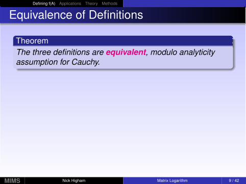
Equivalence of Definitions
Theorem
The three definitions are equivalent, modulo analyticity
assumption for Cauchy.
MIMS Nick Higham Matrix Logarithm 9 / 42

Defining f(A) Applications Theory Methods
Composite Functions
Theorem
f (t) = g(h(t)) ⇒ f (A) = g(h(A)), provided latter matrix
defined.
Corollary
exp(log(A)) = A when log(A) is defined.
MIMS Nick Higham Matrix Logarithm 10 / 42

Defining f(A) Applications Theory Methods
Outline
1 Definition of log(A)
2 Applications
3 Theory
4 Numerical methods
MIMS Nick Higham Matrix Logarithm 11 / 42

Defining f(A) Applications Theory Methods
Application: Markov Models
Time-homogeneous continuous-time Markov process with
transition probability matrix P(t) ∈ Rn×n. Transition intensity
matrix Q related to P by
P(t) = eQt .
Elements of Q satisfy
qij ≥ 0, i 6= j ,n∑
j=1
qij = 0.
Embeddability problem
When does a given stochastic P have
a real logarithm Q that is an intensity
matrix?
MIMS Nick Higham Matrix Logarithm 13 / 42

Defining f(A) Applications Theory Methods
The Average Eye
First order character of optical system characterized by
transference matrix T =[
S0
δ1
]∈ R
5×5, where S ∈ R4×4 is
symplectic: ST JS = J, where J =[
0−I2
I20
].
Average m−1∑m
i=1 Ti is not a transference matrix.
Harris (2005) proposes the average exp(m−1∑m
i=1 log(Ti)).
MIMS Nick Higham Matrix Logarithm 14 / 42

Defining f(A) Applications Theory Methods
The Average Eye
First order character of optical system characterized by
transference matrix T =[
S0
δ1
]∈ R
5×5, where S ∈ R4×4 is
symplectic: ST JS = J, where J =[
0−I2
I20
].
Average m−1∑m
i=1 Ti is not a transference matrix.
Harris (2005) proposes the average exp(m−1∑m
i=1 log(Ti)).
For Hermitian pos def A and B, Arsigny et al. (2007) define
the log-Euclidean mean
E(A, B) = exp(12(log(A) + log(B))).
MIMS Nick Higham Matrix Logarithm 14 / 42

Defining f(A) Applications Theory Methods
Outline
1 Definition of log(A)
2 Applications
3 Theory
4 Numerical methods
MIMS Nick Higham Matrix Logarithm 15 / 42
Defining f(A) Applications Theory Methods
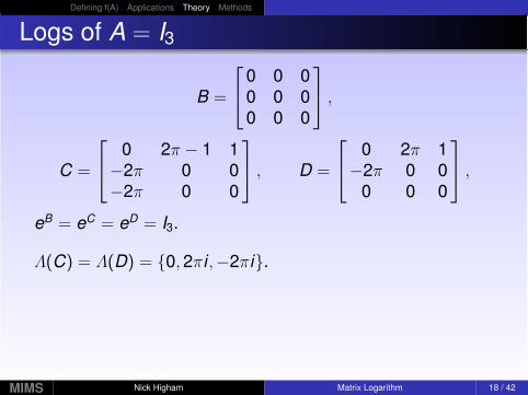
Logs of A = I3
B =
0 0 0
0 0 0
0 0 0
,
C =
0 2π − 1 1
−2π 0 0
−2π 0 0
, D =
0 2π 1
−2π 0 0
0 0 0
,
eB = eC = eD = I3.
Λ(C) = Λ(D) = {0, 2πi ,−2πi}.
MIMS Nick Higham Matrix Logarithm 18 / 42
Defining f(A) Applications Theory Methods
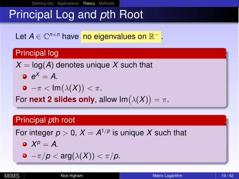
Principal Log and pth Root
Let A ∈ Cn×n have no eigenvalues on R
− .
Principal log
X = log(A) denotes unique X such that
eX = A.
−π < Im(λ(X )
)< π.
For next 2 slides only, allow Im(λ(X )
)= π.
Principal pth root
For integer p > 0, X = A1/p is unique X such that
X p = A.
−π/p < arg(λ(X )) < π/p.
MIMS Nick Higham Matrix Logarithm 19 / 42

Defining f(A) Applications Theory Methods
All Solutions of eX = A
Theorem (Gantmacher)
A ∈ Cn×n nonsing with Jordan canonical form
Z−1AZ = J = diag(J1, J2, . . . , Jp). All solutions to eX = A
are given by
X = Z U diag(L(j1)1 , L
(j2)2 , . . . , L
(jp)p ) U
−1Z−1,
where
L(jk )k = log(Jk(λk)) + 2 jk π i Imk
,
jk ∈ Z arbitrary, and U an arbitrary nonsing matrix that
commutes with J.
MIMS Nick Higham Matrix Logarithm 20 / 42

Defining f(A) Applications Theory Methods
All Solutions of eX = A: Classified
Theorem
A ∈ Cn×n nonsing: p Jordan blocks, s distinct ei’vals.
eX = A has a countable infinity of solutions that are primary
functions of A:
Xj = Zdiag(L(j1)1 , L
(j2)2 , . . . , L
(jp)p )Z−1,
where λi = λk implies ji = jk . If s < p then eX = A has
non-primary solutions
Xj(U) = Z U diag(L(j1)1 , L
(j2)2 , . . . , L
(jp)p ) U
−1Z−1,
where jk ∈ Z arbitrary, U arbitrary nonsing with UJ = JU,
and for each j ∃ i and k s.t. λi = λk while ji 6= jk .
MIMS Nick Higham Matrix Logarithm 21 / 42

Defining f(A) Applications Theory Methods
Logs of A = I3
C =
0 2π − 1 1
−2π 0 0
−2π 0 0
, D =
0 2π 1
−2π 0 0
0 0 0
,
e0 = eC = eD = I3. Λ(C) = Λ(D) = {0, 2πi ,−2πi}.
U =
1 α 0
0 1 α0 0 1
, α ∈ C,
X = U diag(2πi ,−2πi , 0)U−1 = 2π i
1 −2α 2α2
0 1 −α0 0 1
.
MIMS Nick Higham Matrix Logarithm 22 / 42

Defining f(A) Applications Theory Methods
Two Facts on Commuting Matrices
Theorem
If A, B ∈ Cn×n commute then ∃ a unitary U ∈ C
n×n such that
U∗AU and U∗BU are both upper triangular.
MIMS Nick Higham Matrix Logarithm 23 / 42

Defining f(A) Applications Theory Methods
Two Facts on Commuting Matrices
Theorem
If A, B ∈ Cn×n commute then ∃ a unitary U ∈ C
n×n such that
U∗AU and U∗BU are both upper triangular.
Theorem
For A, B ∈ Cn×n, e(A+B)t = eAteBt for all t if and only if
AB = BA.
MIMS Nick Higham Matrix Logarithm 23 / 42

Defining f(A) Applications Theory Methods
When Does log(BC) = log(B) + log(C)?
Theorem
Let B, C ∈ Cn×n commute and have no ei’vals on R
−. If for
every ei’val λj of B and the corr. ei’val µj of C,
|arg λj + arg µj | < π, then log(BC) = log(B) + log(C).
MIMS Nick Higham Matrix Logarithm 24 / 42

Defining f(A) Applications Theory Methods
When Does log(BC) = log(B) + log(C)?
Theorem
Let B, C ∈ Cn×n commute and have no ei’vals on R
−. If for
every ei’val λj of B and the corr. ei’val µj of C,
|arg λj + arg µj | < π, then log(BC) = log(B) + log(C).
Proof. log(B) and log(C) commute, since B and C do.
Therefore
elog(B)+log(C) = elog(B)elog(C) = BC.
Thus log(B) + log(C) is some logarithm of BC. Then
Im(log λj + log µj) = arg λj + arg µj ∈ (−π, π),
so log(B) + log(C) is the principal logarithm of BC.
MIMS Nick Higham Matrix Logarithm 24 / 42

Defining f(A) Applications Theory Methods
Outline
1 Definition of log(A)
2 Applications
3 Theory
4 Numerical methods
MIMS Nick Higham Matrix Logarithm 25 / 42

Defining f(A) Applications Theory Methods
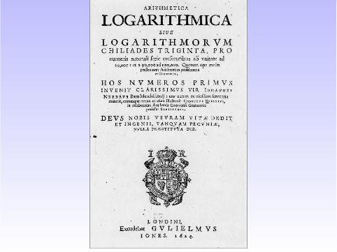
Henry Briggs (1561–1630)
Arithmetica Logarithmica (1624)
Logarithms to base 10 of 1–20,000 and
90,000–100,000 to 14 decimal places.
MIMS Nick Higham Matrix Logarithm 26 / 42

Defining f(A) Applications Theory Methods
Henry Briggs (1561–1630)
Arithmetica Logarithmica (1624)
Logarithms to base 10 of 1–20,000 and
90,000–100,000 to 14 decimal places.
Briggs must be viewed as one of the
great figures in numerical analysis.
—Herman H. Goldstine,
A History of Numerical Analysis (1977)
MIMS Nick Higham Matrix Logarithm 26 / 42


Defining f(A) Applications Theory Methods
Briggs’ Log Method (1617)
log(ab) = log a + log b ⇒ log a = 2 log a1/2.
Use repeatedly:
log a = 2k log a1/2k
.
Write a1/2k= 1 + x and note log(1 + x) ≈ x . Briggs worked
to base 10 and used
log10 a ≈ 2k · log10 e · (a1/2k
− 1).
MIMS Nick Higham Matrix Logarithm 29 / 42

Defining f(A) Applications Theory Methods
Matrix Logarithm
Take B = C in previous theorem:
log A = log(A1/2 · A1/2
)= 2 log A1/2,
since arg λ(A1/2) ∈ (−π/2, π/2).
MIMS Nick Higham Matrix Logarithm 30 / 42

Defining f(A) Applications Theory Methods
Matrix Logarithm
Take B = C in previous theorem:
log A = log(A1/2 · A1/2
)= 2 log A1/2,
since arg λ(A1/2) ∈ (−π/2, π/2).
Use Briggs’ idea: log A = 2k log(A1/2k )
.
MIMS Nick Higham Matrix Logarithm 30 / 42

Defining f(A) Applications Theory Methods
Matrix Logarithm
Take B = C in previous theorem:
log A = log(A1/2 · A1/2
)= 2 log A1/2,
since arg λ(A1/2) ∈ (−π/2, π/2).
Use Briggs’ idea: log A = 2k log(A1/2k )
.
Kenney & Laub’s (1989) inverse scaling and squaring
method:
Bring A close to I by repeated square roots.
Approximate log A1/2kusing an [m/m] Padé
approximant rm(x) ≈ log(1 + x).
Rescale to find log(A).
MIMS Nick Higham Matrix Logarithm 30 / 42

Defining f(A) Applications Theory Methods
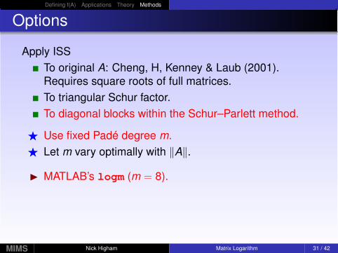
Options
Apply ISS
To original A: Cheng, H, Kenney & Laub (2001).
Requires square roots of full matrices.
To triangular Schur factor.
To diagonal blocks within the Schur–Parlett method.
MIMS Nick Higham Matrix Logarithm 31 / 42

Defining f(A) Applications Theory Methods
Options
Apply ISS
To original A: Cheng, H, Kenney & Laub (2001).
Requires square roots of full matrices.
To triangular Schur factor.
To diagonal blocks within the Schur–Parlett method.
⋆ Use fixed Padé degree m.
⋆ Let m vary optimally with ‖A‖.
MIMS Nick Higham Matrix Logarithm 31 / 42
Defining f(A) Applications Theory Methods
Options
Apply ISS
To original A: Cheng, H, Kenney & Laub (2001).
Requires square roots of full matrices.
To triangular Schur factor.
To diagonal blocks within the Schur–Parlett method.
⋆ Use fixed Padé degree m.
⋆ Let m vary optimally with ‖A‖.
◮ MATLAB’s logm (m = 8).
MIMS Nick Higham Matrix Logarithm 31 / 42

Defining f(A) Applications Theory Methods
Options
Apply ISS
To original A: Cheng, H, Kenney & Laub (2001).
Requires square roots of full matrices.
To triangular Schur factor.
To diagonal blocks within the Schur–Parlett method.
⋆ Use fixed Padé degree m.
⋆ Let m vary optimally with ‖A‖.
◮ MATLAB’s logm (m = 8).
◮ Improved logm.
MIMS Nick Higham Matrix Logarithm 31 / 42

Defining f(A) Applications Theory Methods
Padé Approximants
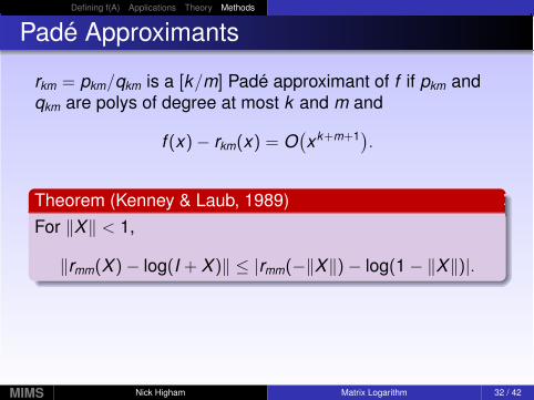
rkm = pkm/qkm is a [k/m] Padé approximant of f if pkm and
qkm are polys of degree at most k and m and
f (x) − rkm(x) = O(xk+m+1
).
For f (x) = log(1 + x),
r11(x) =2x
2 + x,
r22(x) =6x + 3x2
6 + 6x + x2,
r33(x) =60x + 60x2 + 11x3
60 + 90x + 36x2 + 3x3.
MIMS Nick Higham Matrix Logarithm 32 / 42
Defining f(A) Applications Theory Methods
Padé Approximants
rkm = pkm/qkm is a [k/m] Padé approximant of f if pkm and
qkm are polys of degree at most k and m and
f (x) − rkm(x) = O(xk+m+1
).
Theorem (Kenney & Laub, 1989)
For ‖X‖ < 1,
‖rmm(X ) − log(I + X )‖ ≤ |rmm(−‖X‖) − log(1 − ‖X‖)|.
MIMS Nick Higham Matrix Logarithm 32 / 42

Defining f(A) Applications Theory Methods
Algorithmic Ingredients
log A = 2k log(A1/2k )
≈ 2k rm
(A1/2k
− I).
For given A1/2k, error bound determines min m s.t. rm
suff. accurate.
Choose k and m = m(k) to minimize overall cost.
Since(I − A1/2k+1)(
I + A1/2k+1)= I − A1/2k
,
‖I − A1/2k+1
‖ ≈1
2‖I − A1/2k
‖.
Evaluate the partial fraction form
rm(x) =m∑
j=1
α(m)j x
1 + β(m)j x
,
where α(m)j weights and β
(m)j Gauss–Legendre nodes.
MIMS Nick Higham Matrix Logarithm 33 / 42

Defining f(A) Applications Theory Methods
Schur–Parlett Algorithm
H & Davies (2003), funm:
Compute Schur decomposition A = QTQ∗.
Re-order T to block triangular form in which
eigenvalues within a block are “close” and those of
separate blocks are “well separated”.
Evaluate Fii = f (Tii).
Solve the Sylvester equations
Tii Fij − Fij Tjj = FiiTij − TijFjj +
j−1∑
k=i+1
(FikTkj − TikFkj).
Undo the unitary transformations.
MIMS Nick Higham Matrix Logarithm 34 / 42

Defining f(A) Applications Theory Methods
Schur–Parlett Algorithm
H & Davies (2003), funm:
Compute Schur decomposition A = QTQ∗.
Re-order T to block triangular form in which
eigenvalues within a block are “close” and those of
separate blocks are “well separated”.
Evaluate Fii = log(Tii).
Solve the Sylvester equations
Tii Fij − Fij Tjj = FiiTij − TijFjj +
j−1∑
k=i+1
(FikTkj − TikFkj).
Undo the unitary transformations.
MIMS Nick Higham Matrix Logarithm 34 / 42

Defining f(A) Applications Theory Methods
Function of 2 × 2 Block
f
([λ1 t12
0 λ2
])=
f (λ1) t12
f (λ2) − f (λ1)
λ2 − λ1
0 f (λ2)
.
Inaccurate if λ1 ≈ λ2.
Need a better way to compute the divided difference
f [λ2, λ1].
MIMS Nick Higham Matrix Logarithm 35 / 42

Defining f(A) Applications Theory Methods
Log of 2 × 2 Block
log λ2 − log λ1 = log
(λ2
λ1
)+ 2π i U(log λ2 − log λ1)
= log
(1 + z
1 − z
)+ 2π i U(log λ2 − log λ1),
where U = unwinding number, z = (λ2 − λ1)/(λ2 + λ1).
atanh(z) :=1
2log
(1 + z
1 − z
),
MIMS Nick Higham Matrix Logarithm 36 / 42

Defining f(A) Applications Theory Methods
Log of 2 × 2 Block
log λ2 − log λ1 = log
(λ2
λ1
)+ 2π i U(log λ2 − log λ1)
= log
(1 + z
1 − z
)+ 2π i U(log λ2 − log λ1),
where U = unwinding number, z = (λ2 − λ1)/(λ2 + λ1).
atanh(z) :=1
2log
(1 + z
1 − z
),
f12 = t12
2 atanh(z) + 2πiU(log λ2 − log λ1)
λ2 − λ1
.
MIMS Nick Higham Matrix Logarithm 36 / 42

Defining f(A) Applications Theory Methods
Numerical Experiment
◮ 67 test matrices, dimension 2–10.
◮ Evaluated ‖X̂ − log(A)‖F/‖ log(A)‖F .
◮ Notation:
◮ logm: MATLAB 7.4 (R2007a).
◮ logm_new: New version of logm.
◮ iss_schur: Schur decomp then ISS.
◮ iss: ISS on full A.
◮ cond(A) = limǫ→0
max‖E‖2≤ǫ‖A‖2
‖ log(A + E) − log(A)‖2
ǫ‖ log(A)‖2
.
MIMS Nick Higham Matrix Logarithm 37 / 42

Defining f(A) Applications Theory Methods
Performance Profile
1 2 3 4 5 6 7 8 9 100.1
0.2
0.3
0.4
0.5
0.6
0.7
0.8
0.9
1
α
p
logm_newiss_schur
logmiss
MIMS Nick Higham Matrix Logarithm 40 / 42

Defining f(A) Applications Theory Methods
log(A)b
Hale, H & Trefethen, Computing Aα, log(A) and Related
Matrix Functions by Contour Integrals, 2007.
New methods for f (A)b where f has singularities in
(−∞, 0] and A is a matrix with ei’vals on or near (0,∞).
Contour integrals + conformal map + repeated
trapezium rule ⇒ geometric convergence.
MIMS Nick Higham Matrix Logarithm 41 / 42

Defining f(A) Applications Theory Methods
In Conclusion
Matrix logarithm and square root are
archetypal examples of multivalued matrix
functions (LambertW: Corless, Ding, H & Jeffrey,
2007).
Able to classify all logs.
Non-primary logs of interest, but little is
known.
Improvements to inverse scaling and squaring
alg and to logm.
Exploiting structure?
MIMS Nick Higham Matrix Logarithm 42 / 42

Defining f(A) Applications Theory Methods
References I
R. J. Bradford, R. M. Corless, J. H. Davenport, D. J.
Jeffrey, and S. M. Watt.
Reasoning about the elementary functions of complex
analysis.
Annals of Mathematics and Artificial Intelligence,
36:303–318, 2002.
S. H. Cheng, N. J. Higham, C. S. Kenney, and A. J.
Laub.
Approximating the logarithm of a matrix to specified
accuracy.
SIAM J. Matrix Anal. Appl., 22(4):1112–1125, 2001.
MIMS Nick Higham Matrix Logarithm 38 / 42
Defining f(A) Applications Theory Methods
References II
R. M. Corless, H. Ding, N. J. Higham, and D. J. Jeffrey.
The solution of S exp(S) = A is not always the Lambert
W function of A.
In ISSAC ’07: Proceedings of the 2007 International
Symposium on Symbolic and Algebraic Computation,
pages 116–121, New York, 2007. ACM Press.
R. M. Corless and D. J. Jeffrey.
The unwinding number.
ACM SIGSAM Bulletin, 30(2):28–35, June 1996.
MIMS Nick Higham Matrix Logarithm 39 / 42

Defining f(A) Applications Theory Methods
References III
E. D. Dolan and J. J. Moré.
Benchmarking optimization software with performance
profiles.
Math. Programming, 91:201–213, 2002.
F. R. Gantmacher.
The Theory of Matrices, volume one.
Chelsea, New York, 1959.
MIMS Nick Higham Matrix Logarithm 40 / 42

Defining f(A) Applications Theory Methods
References IV
N. Hale, N. J. Higham, and L. N. Trefethen.
Computing Aα, log(A) and related matrix functions by
contour integrals.
MIMS EPrint 2007.xxx, Manchester Institute for
Mathematical Sciences, The University of Manchester,
UK, Aug. 2007.
N. J. Higham.
Evaluating Padé approximants of the matrix logarithm.
SIAM J. Matrix Anal. Appl., 22(4):1126–1135, 2001.
MIMS Nick Higham Matrix Logarithm 41 / 42

Defining f(A) Applications Theory Methods
References V
N. J. Higham.
Functions of Matrices: Theory and Computation.
2008.
Book to appear.
MIMS Nick Higham Matrix Logarithm 42 / 42