ESAIM: M2AN 45 (2011) 779–802 ESAIM: Mathematical Modelling and Numerical Analysis

DOI: 10.1051/m2an/2010102 www.esaim-m2an.org

NUMERICAL ANALYSIS OF A TRANSMISSION PROBLEM WITH SIGNORINICONTACT USING MIXED-FEM AND BEM ∗

Gabriel N. Gatica1, Matthias Maischak

2and Ernst P. Stephan

3

Abstract. This paper is concerned with the dual formulation of the interface problem consisting ofa linear partial differential equation with variable coefficients in some bounded Lipschitz domain Ω inR

n (n ≥ 2) and the Laplace equation with some radiation condition in the unbounded exterior domainΩc := R

n\Ω. The two problems are coupled by transmission and Signorini contact conditions on theinterface Γ = ∂Ω. The exterior part of the interface problem is rewritten using a Neumann to Dirichletmapping (NtD) given in terms of boundary integral operators. The resulting variational formulationbecomes a variational inequality with a linear operator. Then we treat the corresponding numericalscheme and discuss an approximation of the NtD mapping with an appropriate discretization of theinverse Poincare-Steklov operator. In particular, assuming some abstract approximation propertiesand a discrete inf-sup condition, we show unique solvability of the discrete scheme and obtain thecorresponding a-priori error estimate. Next, we prove that these assumptions are satisfied with Raviart-Thomas elements and piecewise constants in Ω, and continuous piecewise linear functions on Γ. Wesuggest a solver based on a modified Uzawa algorithm and show convergence. Finally we present somenumerical results illustrating our theory.

Mathematics Subject Classification. 65N30, 65N38, 65N22, 65F10.

Received January 14, 2008. Revised October 28, 2010.Published online February 21, 2011.

1. Introduction

In this work, we study a transmission problem with an inequality on the interface. This transmission problemcan be seen as a scalar model problem for unilateral contact between a linear elastic unbounded medium anda deformable body. Equivalently, it can be seen as a fluid problem with a semi-permeable membrane. Sucha contact can be described by Signorini boundary conditions. The particular feature of the unilateral problemsis that the mathematical variational statement leads to variational inequalities set on closed convex cones. Themodeling of the non-penetration condition in the discrete setting is of crucial importance.

Keywords and phrases. Raviart-Thomas space, boundary integral operator, Lagrange multiplier.

∗ This research was partially supported by FONDAP and BASAL projects CMM, Universidad de Chile, by Centro de Inves-

tigacion en Ingenierıa Matematica (CI2MA) of the Universidad de Concepcion, by the German Academic Exchange Service(DAAD) through the project 412/HP-hys-rsch, and by the German Research Foundation (DFG) under grant Ste 573/3.1 CI2MA and Departamento de Ingenierıa Matematica, Universidad de Concepcion, Casilla 160-C, Concepcion, Chile.ggatica@ing-mat.udec.cl2 BICOM, Brunel University, UB8 3PH, Uxbridge, UK. matthias.maischak@brunel.ac.uk3 Institut fur Angewandte Mathematik, Leibniz Universitat Hannover, Welfengarten 1, 30167 Hannover, Germany.stephan@ifam.uni-hannover.de

Article published by EDP Sciences c© EDP Sciences, SMAI 2011

780 G.N. GATICA ET AL.

The mathematical foundation for variational inequalities can be found in e.g. [8,12,16]. The numericalanalysis of variational inequalities by finite elements, can be found in, e.g. [4,10,13,15]. An overview on morerecent developments can be found in [19]. Here we take the model problem from [6] with a linear state law inthe interior and combine it with the techniques from e.g. [11] to treat the problem in dual form, which is thenreduced to a bounded domain by the use of the symmetric boundary integral representation of the Neumann toDirichlet map and then is rewritten in a saddle point form to impose weakly the two restrictions for the interiorfield.

Let Ω ⊂ Rn, n ≥ 2 be a bounded domain with Lipschitz boundary Γ. In order to describe mixed boundary

conditions, we let Γ = Γt ∪ Γs where Γs and Γt are nonempty, disjoint, and open in Γ. It is not necessary thatΓt and Γs have a positive distance. Also, we let n denote the unit normal on Γ defined almost everywherepointing from Ω into Ωc := R

n\Ω. Then, given f ∈ L2(Ω) and a matrix-valued function κ ∈ [C(Ω)]n×n, κ = κt,we consider the linear partial differential equations

div(κ∇u) + f = 0 in Ω and Δu = 0 in Ωc, (1.1)

with the radiation condition as |x| → ∞

u(x) = o(1) if n = 2,

u(x) = O(|x|2−n) if n ≥ 3.(1.2)

We assume here that κ induces a strongly elliptic differential operator, that is there exists α > 0 such that

α‖ζ‖2 ≤ (κ(x)ζ) · ζ ∀x ∈ Ω, ∀ζ ∈ Rn. (1.3)

Writing u1 := u in Ω and u2 := u in Ωc, the tractions on Γ are given by the traces (κ∇u1) · n and −∇u2 · n(note that n points into Ωc). Next, given u0 ∈ H1/2(Γ) and t0 ∈ H−1/2(Γ), we consider transmission conditions

u1 = u2 + u0 and (κ∇u1) · n = ∇u2 · n + t0 on Γt, (1.4)

and Signorini conditions

u1 ≤ u2 + u0, (κ∇u1) · n = ∇u2 · n + t0 ≤ 0 and 0 = (κ∇u1) · n (u2 + u0 − u1) on Γs (1.5)

and assume that for n = 2 holds ∫Ω

f(x) dx+∫

Γ

t0 dx = 0. (1.6)

In this way, we look for u1 ∈ H1(Ω) and u2 ∈ W 1(Ωc) satisfying (1.1)–(1.6) in a weak form. The Sobolev spaceW 1(Ωc) is defined at the end of this section.

The purpose of this work is to study a variational formulation, based on the dual-mixed finite elementmethod (dual-mixed FEM) and the boundary element method (BEM), for the above boundary value problem.This includes solvability of the continuous and discrete schemes, and also the associated numerical analysisyielding error estimate and rate of convergence. To this end, (1.1)–(1.6) is written as a saddle point problemgiven on a convex subset, where the original inequality stemming from the Signorini condition is transferred toa Lagrange multiplier.

The main advantage of using a dual-mixed method lies on the possibility of introducing further unknownswith a clear physical meaning. These unknowns are then approximated directly, which avoids any numericalpostprocessing yielding additional sources of error. Also, in this case u becomes an unknown in L2(Ω), whichgives more flexibility to choose the associated finite element subspace. In particular, piecewise constant func-tions become a feasible choice. On the other hand, the transmission conditions of Dirichlet type, being natural

SIGNORINI CONTACT WITH MIXED-FEM AND BEM 781

in this setting, are incorporated directly into the continuous and discrete formulations, thus avoiding noncon-forming Galerkin schemes.

The rest of the paper is organized as follows. In Section 2 we give the dual mixed formulation correspondingto the primal formulation on which the analysis in [6] was based and show its equivalence to the primalformulation. We apply the boundary integral equation method to rewrite the exterior problem, which leads toa dual FEM-BEM minimization problem. Further analysis leads to an equivalent dual mixed-FEM and BEMcoupled formulation, which is the saddle point problem mentioned before. We show the uniqueness of its solutionby proving a continuous inf-sup condition. Then, in Section 4 we deal with the numerical analysis of the discretescheme and discuss the problems resulting from an additional approximation of the inverse Poincare-Steklovoperator, which is essential for its numerical computability. Assuming some abstract approximation propertiesand a discrete inf-sup condition we prove existence and uniqueness of solution for the discrete saddle pointproblem and show an a-priori estimate. Next, in Section 5 we choose Raviart-Thomas elements of order zeroand piecewise constants in the domain, and continuous piecewise linear functions on the boundary, and showthat the discrete inf-sup condition is satisfied for this choice of subspaces. A modified Uzawa solver and theconvergence of our method is presented in Section 6. Finally, in Section 7 we present some numerical resultscorroborating our theory. Namely, in the Examples 7.1 and 7.2 we show that the Uzawa algorithms works wellwith a bounded number of iterations. Example 7.1 also demonstrates that our dual-mixed coupling methodconverges as predicted by Theorem 5.1, i.e. our numerical experiments show that the failure in obtainingoptimal convergence is inherent to the scheme.

In what follows, Hs(Rn), Hs(Ω), H(div; Ω), Hs(Γ) denote the usual Sobolev spaces (see, e.g. [14,17]). Inparticular,

H(div; Ω) ={q ∈ [L2(Ω)]n : div q ∈ L2(Ω)

},

H(div; Ωc) ={q ∈ [L2(Ωc)]n : div q ∈ L2(Ωc)

},

Hs(Γ) ={u|Γ : u ∈ Hs+1/2(Rn)

}(s > 0),

H0(Γ) = L2(Γ), and Hs(Γ) = (H−s(Γ))∗ (s < 0),

where (H−s(Γ))∗ is the dual of H−s(Γ). In addition, 〈·, ·〉 denotes the duality pairing between H−1/2(Γ) andH1/2(Γ) with respect to the L2(Γ)-inner product. Similarly, we let H1/2(Γs) be the subspace of functions inH1/2(Γs) whose extensions by zero to the rest of Γ belong to H1/2(Γ), and denote by H−1/2(Γs) its dual space.Then, 〈·, ·〉Γs stands for the corresponding duality pairing with respect to the L2(Γs)-inner product, and givenμ ∈ H−1/2(Γs), we shall write μ ≤ 0 on Γs if 〈μ, λ〉Γs ≤ 0 for all λ ∈ H1/2(Γs) such that λ ≥ 0. Note, thatH1/2(Γs) coincides with the space H1/2

00 (Γs) in [17].The variational formulation on the unbounded domain Ωc is based on the Beppo-Levi space W 1(Ωc) (see [7])

and takes into account the behaviour at infinity (1.2)

W 1(Ωc) =

{v :

v√1 + |x|2

∈ L2(Ωc),∇v ∈ [L2(Ωc)]n}, n ≥ 3,

W 1(Ωc) =

{v :

v√1 + |x|2 log(2 + |x|2)

∈ L2(Ωc),∇v ∈ [L2(Ωc)]n}, n = 2.

The fundamental difference with the three-dimensional case is that all constant-functions belong to W 1(Ωc), toallow the behaviour at infinity (1.2).

782 G.N. GATICA ET AL.

2. The dual mixed variational formulation

Now, we introduce the dual mixed variational formulation. We introduce the following product spaces

v ∈W 1(Ω ∪ Ωc) ∼= H1(Ω) ×W 1(Ωc) � (v1, v2)

q ∈ H(div; Ω ∪ Ωc) ∼= H(div; Ω) ×H(div; Ωc) � (q1,q2)

q ∈ [L2(Ω ∪ Ωc)]n ∼= [L2(Ω)]n × [L2(Ωc)]n � (q1,q2).

We also introduce jumps[v] = v1 − v2, [q · n] = q1 · n − q2 · n

and two extensions of coefficients and data

κ(x) ={

κ(x), x ∈ Ω,I, elsewhere, f(x) =

{f(x), x ∈ Ω,0, elsewhere.

For all q ∈ H(div; Ω ∪ Ωc) we define the functional

Φ(q) :=12

∫Ω∪Ωc

(κ−1q) · qdx − 〈q1 · n, u0〉 (2.1)

and the subset of admissible functions

C :={q ∈ H(div; Ω ∪ Ωc) : [q · n] = t0 on Γ, q1 · n ≤ 0 on Γs, − div q = f in Ω ∪ Ωc

}.

Note that Φ is convex and coercive. Then we consider the dual mixed problem (P ) given by: Find q0 ∈ C suchthat

Φ(q0) = minq∈C

Φ(q). (2.2)

Theorem 2.1. There exists exactly one solution of (P ).

Proof. Since the set C is convex and closed and Φ is convex and coercive the assertion of the theorem followsfrom standard arguments (cf. [9]). �

To the dual mixed problem (P ) there corresponds the uniquely solvable (up to a constant in 2D) primalproblem (cf. [6]): Find u ∈ C such that

Φ(u) = minv∈C

Φ(v) (2.3)

where for all v ∈ CΦ(v) :=

12

∫Ω∪Ωc

(κ∇v) · ∇v dx−∫

Ω∪Ωc

fv dx− 〈t0, v2〉 (2.4)

and

C :={v ∈ W 1(Ω ∪ Ωc) : [v] = u0 on Γt, [v] ≤ u0 on Γs

}.

The uniqueness up to a constant of (2.3) is due to the identity Φ(v) = Φ(v+c) ∀c ∈ R, which follows from (1.6).We remark that in [6] the primal problem is analyzed for a non-linear differential equation, but the argumentsgiven there are also valid for the case with variable coefficients.

In order to establish the relation between the primal and dual problems (see Thm. 2.2 below), we need thefollowing preliminary result.

SIGNORINI CONTACT WITH MIXED-FEM AND BEM 783

Lemma 2.1. Let J2 : W 1(Ω ∪ Ωc) × [L2(Ω ∪ Ωc)]n → R be the functional defined by

J2(v,q) :=∫

Ω∪Ωc

q · ∇v dx−∫

Ω∪Ωc

fv dx− 〈t0, v2〉

for all v ∈ W 1(Ω ∪ Ωc), q ∈ [L2(Ω ∪ Ωc)]n. Then we have

infv∈C

J2(v,q) ={

〈q1 · n, u0〉 for q ∈ C,

−∞ for q �∈ C.(2.5)

Proof. Since u0 ∈ H1/2(Γ), the extension theorem yields the existence of U0 ∈ H1(Ω ∪ Ωc) such that [U0] = u0

on Γ. Then we defineC0 := {v ∈ W 1(Ω ∪ Ωc) : [v] = 0 on Γt, [v] ≤ 0 on Γs},

and observe that C = U0 + C0. In addition, given q ∈ [L2(Ω ∪ Ωc)]n, J2(·,q) is a continuous linear functionalin W 1(Ω ∪ Ωc), and hence

infv∈C

J2(v,q) = J2(U0,q) + infw∈C0

J2(w,q).

Now, it is not difficult to see that q ∈ C if and only if J2(w,q) ≥ 0 for all w ∈ C0. In fact, the first implicationfollows straightforward from the definition of C. Conversely, let q ∈ [L2(Ω ∪ Ωc)]n such that

J2(w,q) =∫

Ω∪Ωc

q · ∇w dx−∫

Ω∪Ωc

fw dx− 〈t0, w2〉 ≥ 0 ∀w ∈ C0.

Substituting w = ±(ϕ1, ϕ2) ∈ C∞0 (Ω) × C∞

0 (Ωc) in the above inequality we obtain

div q = −f in Ω ∪ Ωc,

and hence q ∈ H(div; Ω ∪ Ωc). Further, we have

J2(w,q) =∫

Ω∪Ωc

q · ∇w dx−∫

Ω∪Ωc

fw dx − 〈t0, w2〉

= (q1,∇w1)[L2(Ω)]n + (div q1, w1)L2(Ω) + (q2,∇w2)[L2(Ωc)]n − 〈t0, w2〉= 〈q1 · n, w1〉 − 〈q2 · n + t0, w2〉, (2.6)

and then for all w ∈ C0 there holds

0 ≤ J2(w,q) = 〈q1 · n, w1〉 − 〈q2 · n + t0, w2〉.

It follows that [q · n] = t0 on Γ and q1 · n ≤ 0 on Γs, and therefore q ∈ C.Next, given q ∈ C we have

J2(v,q) = 〈q1 · n, v1〉 − 〈q2 · n + t0, v2〉 = 〈q1 · n, v1 − v2〉,

and, since v1 − v2 = u0 on Γt, we get

〈q1 · n, v1 − v2〉Γt = 〈q1 · n, u0〉Γt .

Thus, using that q1 · n ≤ 0 on Γs and v1 − v2 ≤ u0 on Γs, we deduce that the infimum will be obtained for theupper bound of v1 − v2, that is

infv∈C

J2(v,q) = 〈q1 · n, u0〉.

784 G.N. GATICA ET AL.

On the other hand, given q �∈ C, the above characterization result implies that there exists w0 ∈ C0 such thatJ2(w0,q) < 0. Then for for all m > 0 we have mw0 ∈ C0 and limm→+∞ J2(mw0,q) = −∞, whence thecorresponding infimum is −∞. �

We are now in a position to provide the following theorem.

Theorem 2.2. Let u ∈ C and q0 ∈ C be the solutions of the primal and dual problems, respectively. Then thereholds

q0 = (κ∇u1,∇u2) and Φ(q0) + Φ(u) = 0. (2.7)

Proof. Let us denote M := [L2(Ω ∪ Ωc)]n, and let J : C ×M ×M → R be the functional defined by

J(v,N,q) :=12

∫Ω∪Ωc

(κN) · N dx−∫

Ω∪Ωc

fv dx+∫

Ω∪Ωc

q · (∇v − N) dx− 〈t0, v2〉

for all v ∈ C, N ∈M , q ∈M .We easily find that

supq1∈[L2(Ω)]n

(q1,∇v1 − N1)[L2(Ω)]n ={

0 for N1 = ∇v1,+∞ for N1 �= ∇v1,

and

supq2∈[L2(Ωc)]n

(q2,∇v2 − N2)[L2(Ωc)]n ={

0 for N2 = ∇v2,+∞ for N2 �= ∇v2,

whence (2.4) givesinfv∈C

Φ(v) = inf[v,N]∈C×M

supq∈M

J(v,N,q). (2.8)

We now denoteS0(q) := inf

[v,N]∈C×MJ(v,N,q) (2.9)

and observe thatS0(q) ≤ inf

v∈CJ(v,∇v,q) = inf

v∈CΦ(v) = Φ(u) ∀q ∈M, (2.10)

which yieldssupq∈M

S0(q) ≤ Φ(u). (2.11)

Furthermore, we can splitS0(q) = inf

N∈MJ1(N,q) + inf

v∈CJ2(v,q) (2.12)

with

J1(N,q) =12

∫Ω∪Ωc

(κN) ·N dx−∫

Ω∪Ωc

q · N dx

and J2 as defined in Lemma 2.1. Next, it is easy to see that

infN∈M

J1(N,q) = −12

∫Ω∪Ωc

(κ−1q) · qdx, (2.13)

and then, using Lemma 2.1, we can write

S0(q) =

⎧⎨⎩ −1

2

∫Ω∪Ωc

(κ−1q) · qdx + 〈q1 · n, u0〉 = −Φ(q) for q ∈ C

−∞ for q �∈ C.(2.14)

SIGNORINI CONTACT WITH MIXED-FEM AND BEM 785

Therefore we haveΦ(u) ≥ sup

q∈MS0(q) = sup

q∈C[−Φ(q)] = − inf

q∈CΦ(q) = −Φ(q0).

We now show that the functional −Φ assumes its maximum at q := κ∇u, which, according to the uniquenessof solution for the dual problem, will imply that κ∇u = q0. Indeed, since the primal problem is equivalent tothe original one, there holds

div(κ∇u) = −f in Ω ∪ Ωc, [(κ∇u) · n] = t0 on Γ, (κ∇u1) · n ≤ 0 on Γs,

which is, respectively,

div q = −f in Ω ∪ Ωc, [q · n] = t0 on Γ, q1 · n ≤ 0 on Γs,

and hence q ∈ C.Now, using that 0 = (κ∇u1) · n (u2 + u0 − u1) on Γs and that u1 = u2 + u0 on Γt, we get

〈(κ∇u1) · n, u1 − u2 − u0〉 = 0, (2.15)

and using div(κ∇u) + f = 0 in Ω ∪ Ωc we obtain∫Ω∪Ωc

(κ∇u) · ∇u dx−∫

Ω∪Ωc

fu dx = 〈(κ∇u1) · n, u1〉 − 〈∇u2 · n, u2〉

= 〈(κ∇u1) · n, u2 + u0〉 − 〈∇u2 · n, u2〉= 〈[(κ∇u) · n], u2〉 + 〈(κ∇u1) · n, u0〉= 〈t0, u2〉 + 〈(κ∇u1) · n, u0〉.

It follows that−

∫Ω∪Ωc

fu dx − 〈t0, u2〉 = −∫

Ω∪Ωc

(κ∇u) · ∇u dx + 〈q1 · n, u0〉, (2.16)

and thereforeΦ(u) =

12

∫Ω∪Ωc

(κ∇u) · ∇u dx−∫

Ω∪Ωc

fu dx− 〈t0, u2〉 = −Φ(q), (2.17)

which ends the proof. �

3. The boundary integral formulation

Now, we collect some known properties of boundary integral operators of the Laplacian and reformulate theexterior part of the original transmission problem with the fundamental solution

G(x, y) = − 12π

log |x− y| if n = 2,

G(x, y) =Γ(n−2

2 )4πn/2

|x− y|2−n if n ≥ 3,

of the Laplacian. For z ∈ Γ and φ ∈ C∞(Γ) we define the operators of the single layer potential V , the doublelayer potential K, its formal adjoint K ′, and the hypersingular integral operator W as

V φ(z) := 2∫

Γ

φ(x)G(z, x) dsx, Kφ(z) := 2∫

Γ

φ(x)∂

∂nxG(z, x) dsx,

K ′φ(z) := 2∫

Γ

φ(x)∂

∂nzG(z, x) dsx, and Wφ(z) := −2

∂

∂nz

∫Γ

φ(x)∂

∂nxG(z, x) dsx.

786 G.N. GATICA ET AL.

We define the operator R by

R :=12(V + (I +K)W−1(I +K ′)) : H−1/2(Γ) → H1/2(Γ). (3.1)

−R is a Neumann to Dirichlet (NtD) map for the exterior domain Ωc and the inverse Poincare-Steklov operator.Two NtD maps can differ by a constant, but the operator R itself is well defined.

The operator W : H1/2(Γ) → H−1/2(Γ) is positive semidefinite, selfadjoint and has a one dimensional kernel(the constant functions). Therefore its range is not H−1/2(Γ) but H−1/2

0 (Γ), which is the polar set of the spaceof constant functions. The range of I + K ′ is also H

−1/20 (Γ), therefore the expression W−1(I + K ′) is well

defined. Because the kernel of I+K is composed of constant functions, the full expression (I+K)W−1(I+K ′)has a precise mathematical meaning. As a consequence the operator R is linear, selfadjoint and elliptic.

A common choice to treat the kernel of the operator W is the subspace of functions in H1/2(Γ) with integralmean zero. However, since this is not optimal from the implementational point of view, we add a least squaresterm to the hypersingular integral operator W . In other words, we define the functional P : H1/2(Γ) → R,

where P (φ) =∫

Γ

φds for all φ ∈ H1/2(Γ), and set

W := W + P ′P : H1/2(Γ) → H−1/2(Γ). (3.2)

The compact perturbation P ′P makes W elliptic.In this way, we can evaluate u := Rt for t ∈ H−1/2(Γ) by computing u = 1

2 (V t+ (I +K)φ), where φ is thesolution of

Wφ = (I +K ′)t. (3.3)Representing the solution φ of (3.3) like φ = φ0 + cφ, such that Pφ0 = 0 and cφ ∈ R, and using that 〈Wφ, 1〉 =〈(I +K ′)t, 1〉, W1 = 0, and K1 = −1, we deduce that 〈P1, Pφ〉 = 0, and consequently, cφ = 0 and φ = φ0 ∈H1/2(Γ)/R is the unique solution of Wφ = (I +K ′)t. Therefore we can replace W by W for the discretizationwithout mentioning it explicitly.

Next, we give a reformulation (P ) of the dual mixed problem (P ) using the operator R (cf. (3.1)). DefiningΨ : H(div; Ω) → R ∪ {∞} by

Ψ(q) :=12

∫Ω

(κ−1q) · qdx +12〈q · n, R(q · n)〉 − 〈q · n, Rt0 + u0〉, (3.4)

on the subset of admissible functions

D :={q ∈ H(div; Ω) : q · n ≤ 0 on Γs, − div q = f in Ω

},

the dual mixed problem (P ) reads: Find qD ∈ D such that

Ψ(qD) = minq∈D

Ψ(q). (3.5)

Theorem 3.1.(a) The dual problems (P ) and (P ) given by (2.2) and (3.5), respectively, are equivalent in the following

sense:(i) If qD ∈ D is a solution of (P ), and qD2 is the gradient of the function u2, which is given by the

representation formula

u2(z) =∫

Γ

v(x)∂

∂nxG(z, x) dsx −

∫Γ

ψ(x)G(z, x) dsx, z ∈ Ωc, (3.6)

SIGNORINI CONTACT WITH MIXED-FEM AND BEM 787

with Cauchy data (v, ψ) := (−R(qD ·n− t0),qD ·n− t0), then (qD,qD2 ) minimizes the functional Φin (2.1).

(ii) If (q01,q

02) ∈ C is the minimizer of Φ on C, then q0

1 is a solution of (P ).(b) (P ) has a unique solution.

Proof. Let qD ∈ D be a solution of (P ) and define u2 and qD2 as in (i). Using the jump relations of potentials,operator identities due to the Calderon projector and the fact that v = −Rψ we obtain ∇u2 ·n = ψ. Thereforeu2 is the only decaying solution of Δu2 = 0 in Ωc with ∇u2 · n = ψ, so u2 = −Rψ = v on Γ. Therefore

‖qD2 ‖2[L2(Ωc)]n = ‖∇u2‖2

[L2(Ωc)]n= 〈ψ,Rψ〉.

A straightforward computation shows

Φ(qD,qD2 ) = Ψ(qD) +12〈t0, Rt0〉. (3.7)

Now, given (q1,q2) ∈ C with Φ(q1,q2) <∞, we know that q2 ∈ H(div; Ωc) and div q2 = 0, and hence thereexists v2 ∈ W 1(Ωc) and q0 ∈ H(div; Ωc) such that q2 = ∇v2 + q0, ∇v2 · n = q1 · n− t0 on Γ, div q0 = 0 in Ωc,and q0 · n = 0 on Γ. Then, we find

Φ(q1,q2) = Ψ(q1) +12〈t0, Rt0〉 +

12‖q0‖2

[L2(Ωc)]n, (3.8)

which implies Φ(q1,q2) ≥ Φ(qD,qD2 ) for all (q1,q2) ∈ C, since (3.7) holds and qD minimizes Ψ. Therefore(qD,qD2 ) minimizes Φ.

Conversely, let (q01,q

02) ∈ C be a minimizer of Φ on C. From (3.8) we know that for all q1 ∈ D we can find

a v2 ∈W 1(Ωc) such that (q1,∇v2) ∈ C and

Φ(q1,∇v2) = Ψ(q1) +12〈t0, Rt0〉. (3.9)

Using Theorem 2.2 we have for all q1 ∈ D

Φ(q01,q

02) = Φ(q0

1,∇u2) = Ψ(q01) +

12〈t0, Rt0〉 ≤ Φ(q1,∇v2) = Ψ(q1) +

12〈t0, Rt0〉,

which yields Ψ(q01) ≤ Ψ(q1), and hence q0

1 minimizes Ψ.The assertion (b) follows from the equivalence in (a) and the unique solvability of (P ). �

Next, we introduce a saddle point formulation (M) of (P ). Indeed, we first define the operator H :H(div; Ω) × L2(Ω) × H1/2(Γs) → R as

H(p, v, μ) := Ψ(p) +∫

Ω

v div p dx+∫

Ω

fv dx + 〈p · n, μ〉Γs (3.10)

for all (p, v, μ) ∈ H(div; Ω) × L2(Ω) × H1/2(Γs), and consider the subset of admissible functions

H1/2+ (Γs) := {μ ∈ H1/2(Γs) : μ ≥ 0}. (3.11)

Then, we define problem (M) as: Find (q, u, λ) ∈ H(div; Ω) × L2(Ω) × H1/2+ (Γs) such that

H(q, u, λ) ≤ H(q, u, λ) ≤ H(q, u, λ) ∀(q, u, λ) ∈ H(div; Ω) × L2(Ω) × H1/2+ (Γs), (3.12)

788 G.N. GATICA ET AL.

which is equivalent (see [9]) to finding a solution (q, u, λ) ∈ H(div; Ω) × L2(Ω) × H1/2+ (Γs) of the following

variational inequality:

a(q,q) + b(q, u) + d(q, λ) = 〈q · n, r〉 ∀q ∈ H(div; Ω), (3.13)

b(q, u) = −∫

Ω

fu dx ∀u ∈ L2(Ω), (3.14)

d(q, λ− λ) ≤ 0 ∀λ ∈ H1/2+ (Γs), (3.15)

where

a(p,q) :=∫

Ω

(κ−1p) · qdx+ 〈q · n, R(p · n)〉 ∀p,q ∈ H(div; Ω), (3.16)

b(q, u) :=∫

Ω

u div qdx ∀(q, u) ∈ H(div; Ω) × L2(Ω), (3.17)

d(q, λ) := 〈q · n, λ〉Γs ∀(q, λ) ∈ H(div; Ω) × H1/2(Γs), (3.18)

and r := Rt0 + u0.Next, we introduce the bilinear form

B(q, (u, λ)) = b(q, u) + d(q, λ) ∀(q, u, λ) ∈ H(div; Ω) × L2(Ω) × H1/2(Γs), (3.19)

and rewrite the variational inequality (3.13)–(3.15) as

a(q,q) +B(q, (u, λ)) = 〈q · n, r〉 ∀q ∈ H(div; Ω) (3.20)

B(q, (u− u, λ− λ)) ≤ −∫

Ω

f(u− u) dx ∀(u, λ) ∈ L2(Ω) × H1/2+ (Γs). (3.21)

Problems (P ) and (M) are connected as follows.

Theorem 3.2. (P ) and (M) are equivalent in the following sense:

(i) If (q, u, λ) solves (M), then q ∈ D is the solution of problem (P ). Additionally, there holds q = κ∇u,u = −R(q · n− t0) + u0 on Γt and λ = −R(q · n− t0) + u0 − u on Γs.

(ii) Let qD ∈ D be the solution of (P ). Then there is a unique solution u ∈ H1(Ω) of the Neumann problem

− div(κ∇u) = f in Ω, (κ∇u) · n = qD · n on Γ

satisfying the additional condition

〈μ, u+R(qD · n − t0) − u0〉 ≥ 0 ∀μ ∈ H−1/2(Γ) with μ ≤ −qD · n on Γs.

Defining λ := −R(qD · n − t0) + u0 − u on Γs, it follows that (qD, u, λ) is a solution of (M).

Proof.(i) If (q, u, λ) is a solution to (M), then (3.14) implies that div q = −f . Then, taking λ = 0 and λ = 2λ,

we find that (3.15) is equivalent to

d(q, λ) = 0 and d(q, λ) ≤ 0 ∀λ ∈ H1/2+ (Γs). (3.22)

SIGNORINI CONTACT WITH MIXED-FEM AND BEM 789

Therefore q ∈ D and Ψ(q) = H(q, u, λ). Since H(q, u, λ) ≤ Ψ(q) for all q ∈ D, then q solves (P ).Finally, elementary arguments show that (3.13) is equivalent to q = κ∇u and to

〈q · n, u+R(q · n) − r〉 + 〈q · n, λ〉Γs = 0 ∀q ∈ H(div; Ω), (3.23)

which is equivalent to the remaining assertions.(ii) Let qD be the solution of (P ). Because qD ∈ D, we know that (3.14) is satisfied and

d(qD, λ) ≤ 0 ∀λ ∈ H1/2+ (Γs). (3.24)

Theorem 2.2 implies that the problem

− div(κ∇u) = f in Ω, (κ∇u) · n = qD · n on Γ, (3.25)

has a solution, unique up to an additive constant. Let us fix the constant by demanding that

〈R(qD · n) + u− r, 1〉 = 0. (3.26)

Using Theorem 2.2 again it is clear that qD = κ∇u. Let us finally define λ = r − u − R(qD · n). Theminimization problem (P ) is equivalent to the variational equation

a(qD,q− qD) − 〈r, (q − qD) · n〉 ≥ 0 ∀q ∈ D. (3.27)

Applying that qD = κ∇u, the definition of λ and the fact that 〈λ, 1〉 = 0, the above variationalinequality implies that

〈λ, c+ (qD − q) · n〉 ≥ 0 ∀q ∈ D ∀c ∈ R. (3.28)

The following claim is the fact that the set{μ ∈ H−1/2(Γ) : μ = c+ (qD − q) · n, q ∈ D, c ∈ R

}(3.29)

contains the following elements: (a) any μ ≥ 0 on Γ; (b) any μ ∈ H−1/2(Γ) such that μ = 0 in Γs, and(c) the two particular elements given by

μ ={

±qD · n, in Γs0 elsewhere. (3.30)

With (a) we prove from (3.28) that λ ≥ 0, with (b) that λ = 0 on Γt and with (c) that d(qD, λ) = 0.Therefore, (3.15) is satisfied and λ ∈ H

1/2+ (Γs). Finally, we have to study

Res(q) := a(qD,q) + b(q, u) + d(q, λ) − 〈q · n, r〉. (3.31)

Using again that qD = κ∇u we prove that

Res(q) = 〈q · n, u+ R(qD · n) − r〉 + 〈q · n, λ〉Γs = 0, (3.32)

so (3.13) is also satisfied and the result is proved.�

790 G.N. GATICA ET AL.

An a-priori estimate for the solution of problem (M) is established next.

Theorem 3.3. There exists a constant C, independent of r (:= Rt0 + u0) and f , such that

‖q‖H(div;Ω) + ‖u‖L2(Ω) + ‖λ‖H1/2(Γs) ≤ C{‖r‖H1/2(Γ) + ‖f‖L2(Ω)

}. (3.33)

Proof. First, we note from the proof of Theorem 2.1 in [2] that there exists a constant β > 0 such that for all(u, λ) ∈ L2(Ω) × H1/2(Γs) there holds

β ‖(u, λ)‖L2(Ω)×H1/2(Γs) ≤ supq∈H(div;Ω)

q �=0

B(q, (u, λ))‖q‖H(div;Ω)

· (3.34)

On the other hand, (3.20) leads to

β ‖(u, λ)‖ ≤ supq∈H(div;Ω)

q �=0

B(q, (u, λ))‖q‖H(div;Ω)

= supq∈H(div;Ω)

q �=0

〈q · n, r〉 − a(q,q)‖q‖H(div;Ω)

≤ C{‖r‖H1/2(Γ) + ‖q‖H(div;Ω)

}. (3.35)

Now, with (3.13)—(3.15) we obtain

a(q, q) = 〈q · n, r〉 − b(q, u) − d(q, λ) = 〈q · n, r〉 + (f, u)L2(Ω)

≤ ‖r‖H1/2(Γ)‖q‖H(div;Ω) + ‖f‖L2(Ω)‖u‖L2(Ω).

Using that div q = −f and (3.35), this yields

‖q‖2H(div;Ω) ≤ c′ · a(q, q) + ‖ div q‖2

L2(Ω)

≤ c′{‖r‖H1/2(Γ)‖q‖H(div;Ω) + ‖f‖L2(Ω)‖u‖L2(Ω)

}+ ‖f‖2

L2(Ω)

≤ C{‖q‖H(div;Ω)

(‖r‖H1/2(Γ) + ‖f‖L2(Ω)

)+ ‖r‖2

H1/2(Γ) + ‖f‖2L2(Ω)

},

and therefore‖q‖2

H(div;Ω) ≤ C{‖r‖2

H1/2(Γ) + ‖f‖2L2(Ω)

}. �

4. General numerical approximation

In this section we treat the numerical approximation for problem (M) by using mixed finite elements in Ωand boundary elements on Γ. For simplicity we assume that Γt and Γs are polygonal hypersurfaces.

Let (Th)h be a family of regular triangulations [3] of the domain Ω by triangles/tetrahedrons T of diameterhT such that h := max{hT : T ∈ Th}. We denote by ρT the diameter of the inscribed circle/sphere in T , and

assume that there exists a constant κ > 0 such that, for any h and for any T in Th, the inequalityhTρT

≤ κ holds.

Moreover we assume that there exists a constant C > 0 such that for any h and for any triangle/tetrahedron Tin Th such that T ∩ ∂Ω is a whole edge/face of T , there holds |T ∩ ∂Ω | ≥ C hn−1, where |T ∩ ∂Ω| denotes thelength/area of T ∩ ∂Ω. This means that the family of triangulations is uniformly regular near the boundary.

We also assume that all the points/curves in Γt ∩ Γs become vertices/edges of Th for all h > 0. Then wedenote by Eh the set of all edges/faces e of Th and put Gh := {e ∈ Eh : e ⊂ Γ}. Further, we let (τh)h bea family of independent regular triangulations of the boundary part Γs by line segments/triangles Δ of diameterhΔ such that h := max{hΔ : Δ ∈ τh}.

SIGNORINI CONTACT WITH MIXED-FEM AND BEM 791

Next, we consider (Xh,h)h,h = (Lh×Hh×H−1/2h ×H1/2

h ×H1/2

s,h)h,h be a family of finite-dimensional subspaces

of X = L2(Ω)×H(div; Ω)×H−1/2(Γ)×H1/2(Γ)/R×H1/2(Γs), subordinated to the corresponding triangulationssuch that the following approximation property holds

limh→0

h→0

{inf

(uh,qh,ψh,φh,λh)∈Xh,h

‖(u,q, ψ, φ, λ) − (uh,qh, ψh, φh, λh)‖X

}= 0 (4.1)

for all (u,q, ψ, φ, λ) ∈ X . In addition, we assume that

{div qh : qh ∈ Hh

}⊆ Lh (4.2)

andH

−1/2h = {qh|Γ · n : qh ∈ Hh} (4.3)

i.e. H−1/2h is the space of normal traces on Γ of the functions in Hh. Also, the subspaces Lh ×H

1/2

s,hand Hh

are supposed to satisfy the usual discrete Babuska-Brezzi condition, which means that there exists β∗ > 0 suchthat

inf(uh,λ

h)∈Lh×H

1/2s,h

(uh,λh) �=0

supqh∈Hhqh �=0

B(qh, (uh, λh))‖qh‖H(div;Ω)‖(uh, λh)‖L2(Ω)×H1/2(Γs)

≥ β∗. (4.4)

Now, we let ih : Lh ↪→ L2(Ω), jh : Hh ↪→ H(div; Ω), kh : H−1/2h ↪→ H−1/2(Γ), lh : H1/2

h ↪→ H1/2(Γ)/Rand mh : H1/2

s,h↪→ H1/2(Γs) denote the canonical imbeddings with their corresponding adjoints i∗h, j

∗h, k

∗h, l

∗h

and m∗h. Let γ : H(div; Ω) → H−1/2(Γ) be the trace operator giving the normal component of functions in

H(div; Ω). Then we have khH−1/2h = γjhHh.

In order to approximate R we define the discrete operators

Rh := k∗hRkh and Rh :=12

(k∗hV kh + k∗h(I +K)lh(l∗hWlh)−1l∗h(I +K ′)kh

).

We remark that the computation of Rh requires the numerical solution of a linear system with a symmetricpositive definite matrix Wh := l∗hWlh. In general, there holds Rh �= Rh because Rh is a Schur complement ofa discretized matrix while Rh is a discretized Schur complement of an operator.

Then, in order to approximate the solution of problem (M), we consider the following Galerkin scheme (Mh)with an approximated bilinear form ah(·, ·): Find (qh, uh, λh) ∈ Hh × Lh ×H

1/2

s,+,hsuch that

ah(qh,qh) + b(qh, uh) + d(qh, λh) = 〈qh · n, rh〉 ∀qh ∈ Hh, (4.5)

b(qh, uh) = −∫

Ω

fuh dx ∀uh ∈ Lh, (4.6)

d(qh, λh − λh) ≤ 0 ∀λh ∈ H1/2

s,+,h, (4.7)

where

H1/2

s,+,h:=

{μ ∈ H

1/2

s,h: μ ≥ 0

}, (4.8)

ah(p,q) =∫

Ω

(κ−1p

)· qdx +

⟨q · n, Rh(p · n)

⟩∀p,q ∈ Hh, (4.9)

792 G.N. GATICA ET AL.

and

rh := k∗h

(12(V + (I +K)lh(l∗hWlh)−1l∗h(I +K ′))t0 + u0

).

Note that the nonconformity of problem (Mh) arises from the bilinear form ah(·, ·) approximating a(·, ·).The following lemma provides bounds for the approximation error introduced by using a discrete Schur

complement.

Lemma 4.1. Let the symmetric operator δr,h be defined for all t ∈ H−1/2(Γ) by

δr,ht :=12(I +K)

(lh(l∗hWlh)−1l∗h −W−1

)(I +K ′)t ∈ H1/2(Γ). (4.10)

Then there exists c0 > 0, independent of h, such that for all t ∈ H−1/2(Γ) there holds

‖δr,ht‖H1/2(Γ) ≤ c0 infφh∈H1/2

h

‖W−1(I +K ′)t− φh‖H1/2(Γ), (4.11)

〈t, δr,ht〉 ≥ 0. (4.12)

Proof. Since W : H1/2(Γ)/R → H−1/2(Γ) is positive definite and we have 〈(I + K ′)t, 1〉 = 〈t, (I + K)1〉 = 0there exists a unique solution z ∈ H1/2(Γ)/R of Wz = (I +K ′)t and zh ∈ H

1/2h of (l∗hWlh)zh = l∗h(I +K ′)t, i.e.

zh is the Galerkin approximation of z. Using the boundedness of (I +K) and the quasi-optimal error estimatewe have

‖δr,ht‖H1/2(Γ) ≤12‖(I +K)‖ · ‖z − lhzh‖H1/2(Γ) ≤ c0 distH1/2(Γ)

(W−1(I +K ′)t,H1/2

h

).

Therefore, we obtain the assertion (4.11), cf. [5], Lemma 9.Additionally, we can write for the error in the energy norm

0 ≤ ‖z − zh‖2W = ‖lhzh‖2

W − ‖z‖2W = t∗(I +K)(lh(l∗hWlh)−1l∗h −W−1)(I +K ′)t = 〈t, δr,ht〉.

This proves assertion (4.12). �

The following lemma provides an upper bound for the difference between the discrete and the continuoussolutions above.

Lemma 4.2. Let (q, u, λ) and (qh, uh, λh) be the solutions of problems (M) and (Mh), respectively. Then thereexists c > 0, independent of h and h, such that

‖u− uh‖2L2(Ω) + ‖λ− λh‖

2H1/2(Γs)

≤ c{‖q− qh‖2

H(div;Ω) + ‖u− uh‖2L2(Ω) + ‖λ− λh‖

2H1/2(Γs)

+ ‖δr,h(t0 − qh · n)‖2H1/2(Γ)

}(4.13)

and

‖q − qh‖2H(div;Ω) ≤ c

{‖q − qh‖2

H(div;Ω) + ‖u− uh‖2L2(Ω) + ‖λ− λh‖

2H1/2(Γs)

− 〈(qh − qh) · n, δr,h(t0 − qh · n)〉 − d(q − qh, λh − λh)}

(4.14)

for all (qh, uh, λh) ∈ Hh × Lh ×H1/2

s,+,h.

SIGNORINI CONTACT WITH MIXED-FEM AND BEM 793

Proof. Given (qh, uh, λh) ∈ Hh × Lh ×H1/2

s,+,h, we observe from (4.5) and (3.13) that

a(q − qh,qh) + 〈qh · n, (R − Rh)(qh · n)〉 + b(qh, u− uh) + d(qh, λ− λh) = 〈qh · n, r − rh〉, (4.15)

whenceb(qh,−uh) + d(qh,−λh) = b(qh,−u) + d(qh,−λ)

− a(q − qh,qh) + 〈qh · n, r − rh − (R − Rh)(qh · n)〉.(4.16)

Note that we have 〈qh · n, r − rh − (R − Rh)(qh · n)〉 = −〈qh · n, δr,h(t0 − qh · n)〉. Similarly, (4.6) and (3.14)give

b(q− qh, uh) = 0. (4.17)Next, applying the discrete inf-sup condition (4.4) and making use of (4.16), we obtain

β∗‖(uh − uh, λh − λh)‖L2(Ω)×H1/2(Γs) ≤ supqh∈Hhqh �=0

b(qh, uh − uh) + d(qh, λh − λh)‖qh‖H(div;Ω)

= supqh∈Hhqh �=0

b(qh, uh − u) + d(qh, λh − λ) − a(q − qh,qh) − 〈qh · n, δr,h(t0 − qh · n)〉‖qh‖H(div;Ω)

≤ C{‖u− uh‖L2(Ω) + ‖λ− λh‖H1/2(Γs) + ‖q− qh‖H(div;Ω) + ‖δr,h(t0 − qh · n)‖H1/2(Γ)

},

which, combined with the triangle inequality applied to (u− uh, λ− λh) = (u−uh, λ−λh)+ (uh− uh, λh− λh),yield (4.13) (see also [13], Thm. 5.1’ and Rem. 5.6).

We now let Y := H(div; Ω) × L2(Ω) × H1/2(Γs) and define the bounded bilinear form A : Y × Y → R by

A((q, u, λ), (q, u, λ)) := a(q,q) + b(q, u) + d(q, λ) − b(q, u) − d(q, λ)

for all (q, u, λ), (q, u, λ) ∈ Y . It follows that

a(q − qh, q− qh) = A((q − qh, u− uh, λ− λh), (q − qh, u− uh, λ− λh))

= A((q − qh, u− uh, λ− λh), (q − qh, u− uh, λ− λh))

+ A((q − qh, u− uh, λ− λh), (qh − qh, uh − uh, λh − λh))

≤ ‖(q − qh, u− uh, λ− λh)‖Y ‖(q − qh, u− uh, λ− λh)‖Y+ A((q − qh, u− uh, λ− λh), (qh − qh, uh − uh, λh − λh)). (4.18)

Then, using (4.15) and (4.17), we obtain

A((

q − qh, u− uh, λ− λh

),(qh − qh, uh − uh, λh − λh

))= − d(q− qh, λh − λh) − 〈(qh − qh) · n, δr,h(t0 − qh · n)〉. (4.19)

Since div(qh − qh) ∈ Lh and (div(q − qh), uh)L2(Ω) = 0 for all uh ∈ Lh, we deduce that

‖ div(q − qh)‖L2(Ω) ≤ ‖ div(q − qh)‖L2(Ω) ≤ ‖q− qh‖H(div;Ω) ∀qh ∈ Hh. (4.20)

Finally, combining (4.18), (4.19), (4.20) and (4.13), and applying the generalized Cauchy-Schwarz inequality,we arrive at (4.14). �

794 G.N. GATICA ET AL.

The main result of this section is established as follows.

Theorem 4.1. Let (q, u, λ) and (qh, uh, λh) be the solutions of problems (M) and (Mh), respectively. Defineφ := W−1(I + K ′)(t0 − q · n). Then there exists c > 0, independent of h and h, such that the following Ceatype estimate holds

‖q− qh‖H(div;Ω) + ‖u− uh‖L2(Ω) + ‖λ− λh‖H1/2(Γs)

≤ c

{inf

qh∈Hh

‖q− qh‖H(div;Ω) + infuh∈Lh

‖u− uh‖L2(Ω) + infλh∈H1/2

s,+,h

‖λ− λh‖1/2

H1/2(Γs)

+ infφh∈H1/2

h

‖φ− φh‖H1/2(Γ)

}. (4.21)

Proof. We apply the estimates provided in Lemmas 4.2 and 4.1. Due to (4.7) and (3.15), the term −d(q −qh, λh − λh) given in Lemma 4.2 is estimated as follows

− d(q − qh, λh − λh) = d(q, λh − λh) + d(qh, λh − λh)

≤ d(q, λh − λh) = d(q, λh − λ) + d(q, λ− λh) ≤ d(q, λ− λh).

Then we estimate the term d(q, λ−λh) by ‖q‖H(div;Ω)‖λ−λh‖H1/2(Γs) and note that ‖q‖H(div;Ω) is bounded due

to Theorem 3.3. Due to Lemma 4.1 the term ‖δr,h(t0−qh ·n)‖2H1/2(Γ)

is bounded by c0{

infφh∈H1/2

h

‖W−1(I+K ′)

(t0 − q · n) − φh‖H1/2(Γ) + ‖q · n − qh · n‖H−1/2(Γ)

}. Then, we can estimate

−〈(qh − qh) · n, δr,h(t0 − qh · n)〉= −〈qh · n − q · n + q · n− qh · n, δr,h(t0 − q · n + q · n − qh · n)〉= −〈(qh − q) · n, δr,h(t0 − q · n)〉 − 〈(qh − q) · n, δr,h(q · n− qh · n)〉

−〈(q − qh) · n, δr,h(t0 − q · n)〉 − 〈(q − qh) · n, δr,h(q · n− qh · n)〉

≤ 12‖q − qh‖2

H(div;Ω) +12‖δr,h(t0 − q · n)‖2

H1/2(Γ)

+12ε

‖q − qh‖2H(div;Ω) +

ε

2‖δr,h(q · n− qh · n)‖2

H1/2(Γ)

+ε

2‖q− qh‖2

H(div;Ω) +12ε

‖δr,h(t0 − q · n)‖2H1/2(Γ).

Note, due to Lemma 4.1 we have −〈(q− qh) ·n, δr,h(q ·n− qh ·n)〉 ≤ 0. Finally, after choosing a suitable ε > 0we take the infimum. �

5. Numerical approximation

In this section we apply the general approximation theory of the previous section to a particular choice offinite dimensional subspaces. In order to define them, we first consider an element T of a regular triangulationTh of the domain Ω, and for each integer k ≥ 0, we denote by P k(T ) the space of polynomial functions ofdegree ≤ k on T . A similar definition holds for P k(e) where e is an edge of Th. We define the lowest-orderRaviart-Thomas space

RT0(Th) := {q ∈ H(div; Ω) : q|T ∈ [P 0(T )]n + xP 0(T ) ∀T ∈ Th}

SIGNORINI CONTACT WITH MIXED-FEM AND BEM 795

where x = (x1, . . . , xn)T. Then, we define the subspaces

Hh := RT0(Th),Lh := {vh ∈ L2(Ω) : vh|T ∈ P 0(T ) ∀T ∈ Th},

H1/2

s,h:= {λh ∈ C(Γs) : λh|e ∈ P 1(e) ∀e ∈ τh},

H−1/2h := {ψh ∈ L2(Γ) : ψh|e ∈ P 0(e) ∀e ∈ Gh},

H−1/2s,h := {ψh ∈ L2(Γs) : ψh|e ∈ P 0(e) ∀e ∈ Gh}.

Note, H−1/2h is the space of normal traces on Γ of the functions in Hh, and H−1/2

s,h is the space of normal traceson Γs of the functions in Hh.

In order to obtain the following inf-sup condition for the bilinear form B(·, (·, ·)) we must impose someadditional restrictions on the discrete spaces which are the direct 3d analogues of the assumptions for the 2dcase treated in [2].

Lemma 5.1. Let (Th)h be uniformly regular near Γs, which means that there exists C > 0, independent of h,such that min{hT : T ∈ Th , T ∩Γs �= φ } ≥ C h. Furthermore, let the partition (τh) of Γs be uniformly regular,that is there exists C > 0 such that min{hΔ : Δ ∈ τh} ≥ Ch. Then there exist constants C0, β > 0, independentof h and h, such that for all h ≤ C0h

inf(uh,λh)∈Lh×H1/2

s,h\{0}

supqh∈Hh\{0}

B(qh, (uh, λh))‖qh‖H(div;Ω)‖(uh, λh)‖L2(Ω)×H1/2(Γs)

≥ β > 0. (5.1)

Proof. The assertion is shown by generalizing the results in [2], covering the 2d situation, to the 3d situationgiven here. We omit the details for brevity. �

This section is completed with a result on the rate of convergence of the nonconforming Galerkin scheme(Mh). For this, we need the following approximation properties of the subspaces Lh, Hh, H

−1/2h , H1/2

h , andH

1/2

s,h, respectively (see, e.g. [1,3,18]):

For all v ∈ H1(Ω) there exists vh ∈ Lh such that

‖v − vh‖L2(Ω) ≤ C h ‖v‖H1(Ω). (5.2)

For all q ∈ [H1(Ω)]n with div q ∈ H1(Ω), there exists qh ∈ Hh such that

‖q − qh‖H(div;Ω) ≤ C h{‖q‖[H1(Ω)]n + ‖ divq‖H1(Ω)

}. (5.3)

For all ψ ∈ H1/2(Γ), there exists ψh ∈ H−1/2h such that

‖ψ − ψh‖H−1/2(Γ) ≤ C h ‖ψ‖H1/2(Γ). (5.4)

For all φ ∈ H3/2(Γ), there exists φh ∈ H1/2h such that

‖φ− φh‖H1/2(Γ) ≤ C h ‖φ‖H3/2(Γ). (5.5)

For all λ ∈ H3/2(Γs), there exists λh ∈ H1/2

s,hsuch that

‖λ− λh‖H1/2(Γs) ≤ C h ‖λ‖H3/2(Γs). (5.6)

796 G.N. GATICA ET AL.

Theorem 5.1. Let (q, u, λ) and (qh, uh, λh) be the solutions of problems (M) and (Mh), respectively. Assumethat q ∈ [H1(Ω)]n, div q ∈ H1(Ω), u ∈ L2(Ω), λ ∈ H3/2(Γs), φ := W−1(I +K ′)(t0 − q · n) ∈ H3/2(Γ). Thenthe following a priori error estimate holds

‖q− qh‖H(div;Ω) + ‖u− uh‖L2(Ω) + ‖λ− λh‖H1/2(Γs)

≤ C h{‖q‖[H1(Ω)]n + ‖ div q‖H1(Ω) + ‖u‖H1(Ω) + ‖φ‖H3/2(Γ)

}+ C h1/2 ‖λ‖1/2

H3/2(Γs)

with a constant C independent of h and h, with h ≤ C0h.

Proof. The estimates for q, u, and λ follow directly from Theorem 4.1, the assumed regularity of the solutionof (M) and the approximation properties (5.2), (5.3), (5.5) and (5.6). �

6. Solvers for FEM-BEM dual-mixed coupling problems

As solver for the discretized saddle point problem (Mh) we take a modified Uzawa algorithm that utilizesthe equation for the Lagrange multiplier u. First, we introduce a projector Ph : H1/2

s,h→ H

1/2

s,+,hand a linear

mapping Φ : H(div; Ω) → H1/2

s,h⊂ H1/2(Γs), which satisfy for given λ ∈ H

1/2

s,hand q ∈ H(div; Ω)

(Phλ− λ, λh − Phλ)H1/2(Γs) ≥ 0 ∀λh ∈ H1/2

s,+,h, (6.1)

andd(q, λh) = (λh,Φ(q))H1/2(Γs)

∀λh ∈ H1/2

s,h. (6.2)

Therefore‖Φ(q)‖2

H1/2(Γs)= d(q,Φ(q)) = 〈q · n,Φ(q)〉Γs ≤ ‖q · n‖H−1/2(Γs) ‖Φ(q)‖H1/2(Γs),

yielding‖Φ(q)‖H1/2(Γs) ≤ ‖q · n‖H−1/2(Γs) ≤ ‖q‖H(div;Ω) ∀q ∈ H(div; Ω), (6.3)

which proves the continuity of the linear mapping Φ.

Algorithm 6.1 (modified Uzawa).

1. Choose an initial λ(0) ∈ H1/2

s,+,h.

2. Given λ(n) ∈ H1/2

s,+,h, find (q(n), u(n)) ∈ Hh × Lh such that

ah(q(n),qh) + b(qh, u(n)) = 〈rh,qh · n〉 − d(qh, λ(n)) ∀qh ∈ Hh, (6.4)

b(q(n), uh) = − (f, uh)L2(Ω) ∀uh ∈ Lh. (6.5)

3. Compute λ(n+1) byλ(n+1) = Ph(λ

(n) + �Φ(q(n))). (6.6)

4. Check for some stopping criterion and if it is not fulfilled, then go to step 2.

The convergence of this algorithm is established in the following theorem.

Theorem 6.1. With 0 < � < 2 the modified Uzawa algorithm converges towards the solution of the discreteproblem (Mh) for arbitrary starting value λ0 ∈ H

1/2

s,+,h.

SIGNORINI CONTACT WITH MIXED-FEM AND BEM 797

Proof. Let (qh, uh, λh) ∈ Hh × Lh ×H1/2

s,+,hsolve problem (Mh). Then (4.7) and (6.2) give

(λh − λh, λh − (λh + �Φ(qh)))H1/2(Γs) ≥ 0 ∀λh ∈ H1/2

s,+,h,

which means thatλh = Ph(λh + �Φ(qh)). (6.7)

Therefore, it follows that

‖λ(n+1) − λh‖2H1/2(Γs)

= ‖Ph(λ(n) + �Φ(q(n))) − Ph(λh + �Φ(qh))‖2H1/2(Γs)

≤ ‖λ(n) − λh‖2H1/2(Γs)

+ 2 � d(q(n) − qh, λ(n) − λh) + �2 ‖Φ(q(n)) − Φ(qh)‖2H1/2(Γs)

.

Then, using (4.5) and (6.4), we obtain

d(q(n) − qh, λ(n) − λh) = − ah(q(n) − qh,q(n) − qh),

and due to (4.6) and (6.5) we have for q(n) − qh ∈ Hh that

(div(q(n) − qh), uh)L2(Ω) = 0 ∀uh ∈ Lh,

which gives div(q(n) − qh) = 0. Thus, there holds

d(q(n) − qh, λ(n) − λh) = − ah(q(n) − qh,q(n) − qh) ≤ −‖q(n) − qh‖2L2(Ω) = −‖q(n) − qh‖2

H(div;Ω).

Together with (6.3) this yields

‖λ(n+1) − λh‖2H1/2(Γs)

≤ ‖λ(n) − λh‖2H1/2(Γs)

− � (2 − �) ‖q(n) − qh‖2H(div;Ω). (6.8)

Thus ‖λ(n)−λh‖2H1/2(Γs)

is monotonically decreasing and bounded from below, and therefore convergent. Hence,we get

0 ≤ � (2 − �) ‖q(n) − qh‖2H(div;Ω) ≤ ‖λ(n) − λh‖

2H1/2(Γs)

− ‖λ(n+1) − λh‖2H1/2(Γs)

,

which goes to 0 as n→ ∞, and therefore

limn→∞ ‖q(n) − qh‖2

H(div;Ω) = 0. (6.9)

Now, from (4.5) and (6.4) we have

B(qh, (u(n) − uh, λ(n) − λh)) = ah(qh − q(n),qh) ∀qh ∈ Hh.

Applying the discrete inf-sup condition (5.1) for B we obtain

β ‖(u(n), λ(n)) − (uh, λh)‖L2(Ω)×H1/2(Γs) ≤ supqh∈Hh\{0}

B(qh, (u(n) − uh, λ(n) − λh))

‖qh‖H(div;Ω)

= supqh∈Hh\{0}

ah(qh − q(n),qh)‖qh‖H(div;Ω)

≤ C ‖qh − q(n)‖H(div;Ω),

which shows with (6.9) the claimed convergence of (u(n), λ(n)). �

798 G.N. GATICA ET AL.

Ω

Ωc

Γt

Γs

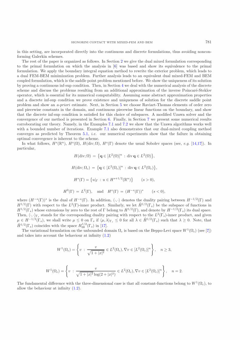
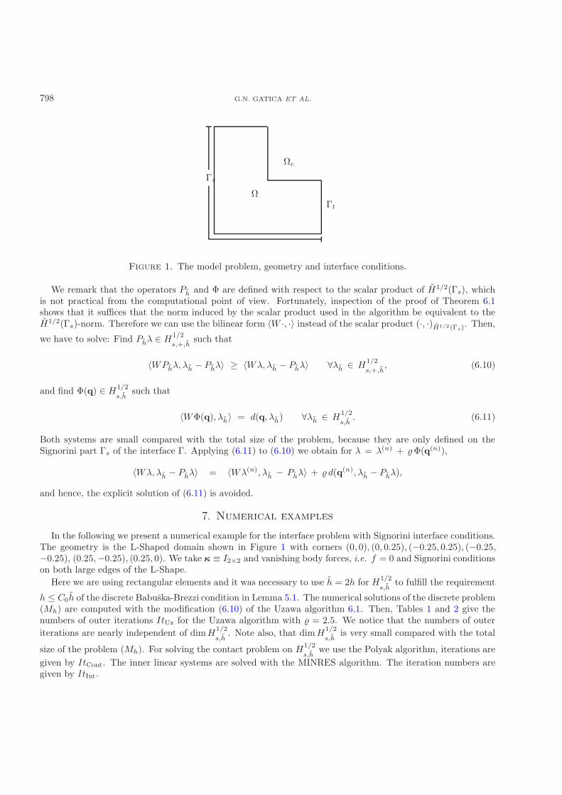
Figure 1. The model problem, geometry and interface conditions.

We remark that the operators Ph and Φ are defined with respect to the scalar product of H1/2(Γs), whichis not practical from the computational point of view. Fortunately, inspection of the proof of Theorem 6.1shows that it suffices that the norm induced by the scalar product used in the algorithm be equivalent to theH1/2(Γs)-norm. Therefore we can use the bilinear form 〈W ·, ·〉 instead of the scalar product (·, ·)H1/2(Γs). Then,

we have to solve: Find Phλ ∈ H1/2

s,+,hsuch that

〈WPhλ, λh − Phλ〉 ≥ 〈Wλ, λh − Phλ〉 ∀λh ∈ H1/2

s,+,h, (6.10)

and find Φ(q) ∈ H1/2

s,hsuch that

〈WΦ(q), λh〉 = d(q, λh) ∀λh ∈ H1/2

s,h. (6.11)

Both systems are small compared with the total size of the problem, because they are only defined on theSignorini part Γs of the interface Γ. Applying (6.11) to (6.10) we obtain for λ = λ(n) + �Φ(q(n)),

〈Wλ, λh − Phλ〉 = 〈Wλ(n), λh − Phλ〉 + � d(q(n), λh − Phλ),

and hence, the explicit solution of (6.11) is avoided.

7. Numerical examples

In the following we present a numerical example for the interface problem with Signorini interface conditions.The geometry is the L-Shaped domain shown in Figure 1 with corners (0, 0), (0, 0.25), (−0.25, 0.25), (−0.25,−0.25), (0.25,−0.25), (0.25, 0). We take κ ≡ I2×2 and vanishing body forces, i.e. f = 0 and Signorini conditionson both large edges of the L-Shape.

Here we are using rectangular elements and it was necessary to use h = 2h for H1/2

s,hto fulfill the requirement

h ≤ C0h of the discrete Babuska-Brezzi condition in Lemma 5.1. The numerical solutions of the discrete problem(Mh) are computed with the modification (6.10) of the Uzawa algorithm 6.1. Then, Tables 1 and 2 give thenumbers of outer iterations ItUz for the Uzawa algorithm with � = 2.5. We notice that the numbers of outeriterations are nearly independent of dimH

1/2

s,h. Note also, that dimH

1/2

s,his very small compared with the total

size of the problem (Mh). For solving the contact problem on H1/2

s,hwe use the Polyak algorithm, iterations are

given by ItCont. The inner linear systems are solved with the MINRES algorithm. The iteration numbers aregiven by ItInt.

SIGNORINI CONTACT WITH MIXED-FEM AND BEM 799

−.3845E+00−.3527E+00−.3209E+00−.2892E+00−.2574E+00−.2256E+00−.1938E+00−.1621E+00−.1303E+00−.9851E−01−.6674E−01−.3496E−01−.3183E−020.2859E−010.6037E−010.9215E−010.1239E+00

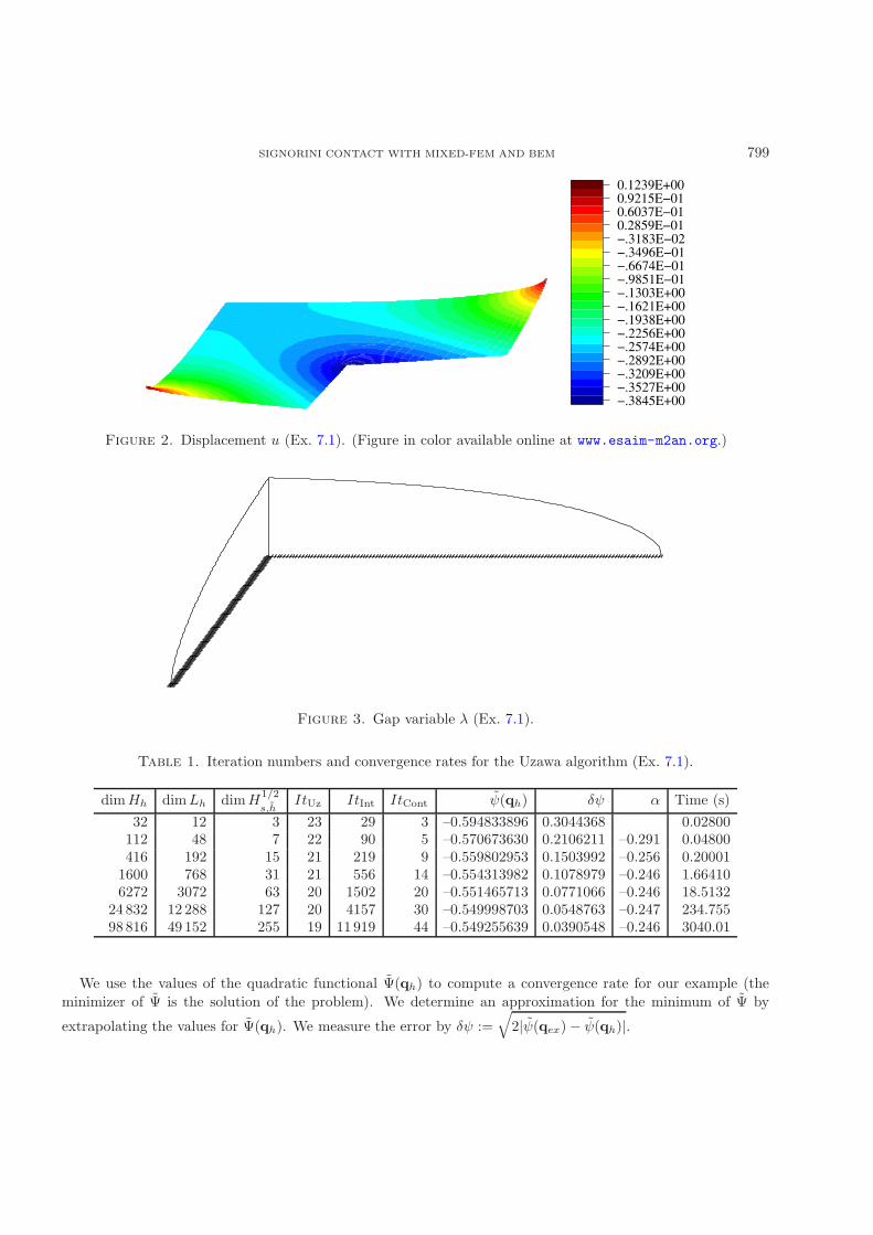
Figure 2. Displacement u (Ex. 7.1). (Figure in color available online at www.esaim-m2an.org.)

Figure 3. Gap variable λ (Ex. 7.1).

Table 1. Iteration numbers and convergence rates for the Uzawa algorithm (Ex. 7.1).

dimHh dimLh dimH1/2

s,hItUz ItInt ItCont ψ(qh) δψ α Time (s)

32 12 3 23 29 3 –0.594833896 0.3044368 0.02800112 48 7 22 90 5 –0.570673630 0.2106211 –0.291 0.04800416 192 15 21 219 9 –0.559802953 0.1503992 –0.256 0.20001

1600 768 31 21 556 14 –0.554313982 0.1078979 –0.246 1.664106272 3072 63 20 1502 20 –0.551465713 0.0771066 –0.246 18.5132

24 832 12 288 127 20 4157 30 –0.549998703 0.0548763 –0.247 234.75598 816 49 152 255 19 11 919 44 –0.549255639 0.0390548 –0.246 3040.01

We use the values of the quadratic functional Ψ(qh) to compute a convergence rate for our example (theminimizer of Ψ is the solution of the problem). We determine an approximation for the minimum of Ψ by

extrapolating the values for Ψ(qh). We measure the error by δψ :=√

2|ψ(qex) − ψ(qh)|.

800 G.N. GATICA ET AL.

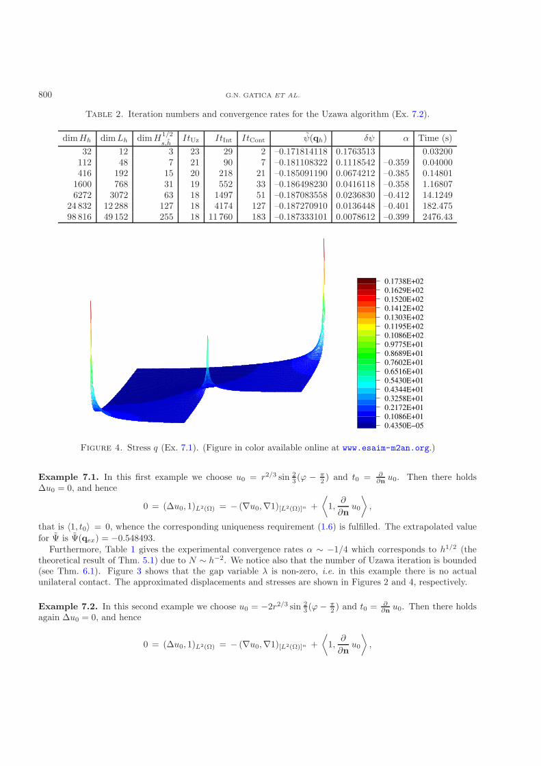
Table 2. Iteration numbers and convergence rates for the Uzawa algorithm (Ex. 7.2).

dimHh dimLh dimH1/2

s,hItUz ItInt ItCont ψ(qh) δψ α Time (s)

32 12 3 23 29 2 –0.171814118 0.1763513 0.03200112 48 7 21 90 7 –0.181108322 0.1118542 –0.359 0.04000416 192 15 20 218 21 –0.185091190 0.0674212 –0.385 0.14801

1600 768 31 19 552 33 –0.186498230 0.0416118 –0.358 1.168076272 3072 63 18 1497 51 –0.187083558 0.0236830 –0.412 14.1249

24 832 12 288 127 18 4174 127 –0.187270910 0.0136448 –0.401 182.47598 816 49 152 255 18 11 760 183 –0.187333101 0.0078612 –0.399 2476.43

0.4350E−050.1086E+010.2172E+010.3258E+010.4344E+010.5430E+010.6516E+010.7602E+010.8689E+010.9775E+010.1086E+020.1195E+020.1303E+020.1412E+020.1520E+020.1629E+020.1738E+02

Figure 4. Stress q (Ex. 7.1). (Figure in color available online at www.esaim-m2an.org.)

Example 7.1. In this first example we choose u0 = r2/3 sin 23 (ϕ − π

2 ) and t0 = ∂∂n u0. Then there holds

Δu0 = 0, and hence

0 = (Δu0, 1)L2(Ω) = − (∇u0,∇1)[L2(Ω)]n +⟨

1,∂

∂nu0

⟩,

that is 〈1, t0〉 = 0, whence the corresponding uniqueness requirement (1.6) is fulfilled. The extrapolated valuefor Ψ is Ψ(qex) = −0.548493.

Furthermore, Table 1 gives the experimental convergence rates α ∼ −1/4 which corresponds to h1/2 (thetheoretical result of Thm. 5.1) due to N ∼ h−2. We notice also that the number of Uzawa iteration is bounded(see Thm. 6.1). Figure 3 shows that the gap variable λ is non-zero, i.e. in this example there is no actualunilateral contact. The approximated displacements and stresses are shown in Figures 2 and 4, respectively.

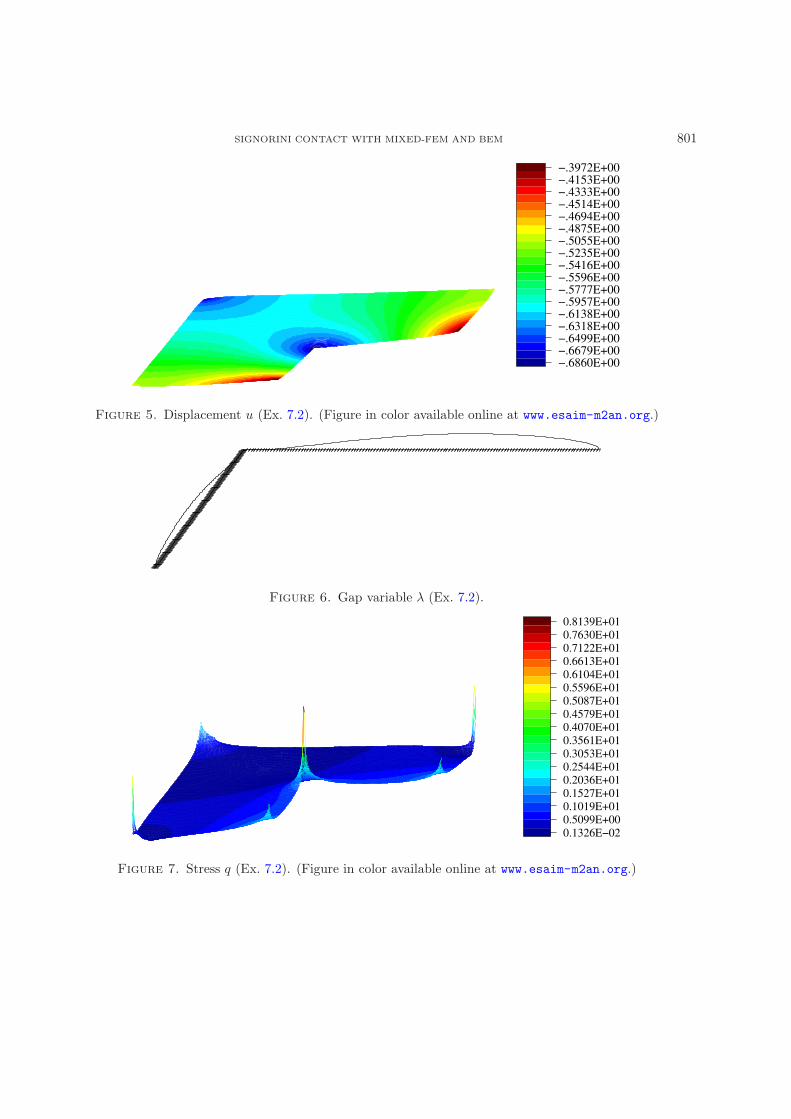
Example 7.2. In this second example we choose u0 = −2r2/3 sin 23 (ϕ − π

2 ) and t0 = ∂∂n u0. Then there holds

again Δu0 = 0, and hence

0 = (Δu0, 1)L2(Ω) = − (∇u0,∇1)[L2(Ω)]n +⟨

1,∂

∂nu0

⟩,

SIGNORINI CONTACT WITH MIXED-FEM AND BEM 801

−.6860E+00−.6679E+00−.6499E+00−.6318E+00−.6138E+00−.5957E+00−.5777E+00−.5596E+00−.5416E+00−.5235E+00−.5055E+00−.4875E+00−.4694E+00−.4514E+00−.4333E+00−.4153E+00−.3972E+00

Figure 5. Displacement u (Ex. 7.2). (Figure in color available online at www.esaim-m2an.org.)

Figure 6. Gap variable λ (Ex. 7.2).

0.1326E−020.5099E+000.1019E+010.1527E+010.2036E+010.2544E+010.3053E+010.3561E+010.4070E+010.4579E+010.5087E+010.5596E+010.6104E+010.6613E+010.7122E+010.7630E+010.8139E+01

Figure 7. Stress q (Ex. 7.2). (Figure in color available online at www.esaim-m2an.org.)

802 G.N. GATICA ET AL.

that is 〈1, t0〉 = 0, whence the corresponding uniqueness requirement (1.6) is fulfilled. The extrapolated valuefor Ψ is Ψ(qex) = −0.187364.

Furthermore, Table 2 gives the experimental convergence rates α ∼ −0.4 which corresponds to h0.8 due toN ∼ h−2. Again the number of Uzawa iterations is bounded. Figure 6 shows that the gap variable λ vanishesnear the corner (− 1

4 ,−14 ), i.e. in this example there is unilateral contact. The approximated displacements and

stresses are shown in Figures 5 and 7, respectively.

Acknowledgements. The authors would like to thank the referees for their very helpful comments.

References

[1] I. Babuska and A.K. Aziz, Survey Lectures on the Mathematical Foundations of the Finite Element Method. Academic Press,New York (1972) 3–359.

[2] I. Babuska and G.N. Gatica, On the mixed finite element method with Lagrange multipliers. Numer. Methods Partial Differ.Equ. 19 (2003) 192–210.

[3] F. Brezzi and M. Fortin, Mixed and Hybrid Finite Element Methods. Springer-Verlag (1991).[4] F. Brezzi, W.W. Hager and P.-A. Raviart, Error estimates for the finite element solution of variational inequalities. Numer.

Math. 28 (1977) 431–443.[5] C. Carstensen, Interface problem in holonomic elastoplasticity. Math. Methods Appl. Sci. 16 (1993) 819–835.[6] C. Carstensen and J. Gwinner, FEM and BEM coupling for a nonlinear transmission problem with Signorini contact. SIAM

J. Numer. Anal. 34 (1997) 1845–1864.[7] R. Dautray and J.-L. Lions, Mathematical Analysis and Numerical Methods for Science and Technology 4. Springer (1990).[8] G. Duvaut and J. Lions, Inequalities in Mechanics and Physics. Springer, Berlin (1976).

[9] I. Ekeland and R. Temam, Analyse Convexe et Problemes Variationnels. Etudes mathematiques, Dunod, Gauthier-Villars,Paris-Bruxelles-Montreal (1974).

[10] R.S. Falk, Error estimates for the approximation of a class of variational inequalities. Math. Comput. 28 (1974) 963–971.[11] G. Gatica and W. Wendland, Coupling of mixed finite elements and boundary elements for linear and nonlinear elliptic

problems. Appl. Anal. 63 (1996) 39–75.[12] R. Glowinski, J.-L. Lions and R. Tremolieres, Numerical Analysis of Variational Inequalities, Studies in Mathematics and its

Applications 8. North-Holland Publishing Co., Amsterdam-New York (1981).[13] I. Hlavacek, J. Haslinger, J. Necas and J. Lovisek, Solution of Variational Inequalities in Mechanics, Applied Mathematical

Sciences 66. Springer-Verlag (1988).[14] L. Hormander, Linear Partial Differential Operators. Springer-Verlag, Berlin (1969).[15] N. Kikuchi and J. Oden, Contact Problems in Elasticity: a Study of Variational Inequalities and Finite Element Methods.

SIAM, Philadelphia (1988).[16] D. Kinderlehrer and G. Stampacchia, An Introduction to Variational Inequalities and their Applications. Academic Press

(1980).[17] J. Lions and E. Magenes, Non-Homogeneous Boundary Value Problems and Applications I. Springer-Verlag, Berlin (1972).[18] J.E. Roberts and J.M. Thomas, Mixed and Hybrid Methods, in Handbook of Numerical Analysis II, P.G. Ciarlet and J.-L. Lions

Eds., North-Holland, Amsterdam (1991) 523–639.[19] Z.-H. Zhong, Finite Element Procedures for Contact-Impact Problems. Oxford University Press (1993).