Number of discernible object colors is a conundrumrit-mcsl.org/fairchild//PDFs/PAP32.pdf · Number...

Number of discernible object colors is a conundrum

Kenichiro Masaoka,1,2,* Roy S. Berns,2 Mark D. Fairchild,2 and Farhad Moghareh Abed2

1NHK Science & Technology Research Laboratories, Tokyo 157-8510, Japan2Munsell Color Science Laboratory, Chester F. Carlson Center for Imaging Science, Rochester Institute of Technology,

Rochester, New York 14623, USA*Corresponding author: masaoka.k‑[email protected]

Received June 15, 2012; revised December 19, 2012; accepted December 24, 2012;posted January 2, 2013 (Doc. ID 169396); published January 31, 2013

Widely varying estimates of the number of discernible object colors have been made by using various methodsover the past 100 years. To clarify the source of the discrepancies in the previous, inconsistent estimates, thenumber of discernible object colors is estimated over a wide range of color temperatures and illuminance levelsusing several chromatic adaptation models, color spaces, and color difference limens. Efficient and accuratemodels are used to compute optimal-color solids and count the number of discernible colors. A comprehensivesimulation reveals limitations in the ability of current color appearance models to estimate the number ofdiscernible colors even if the color solid is smaller than the optimal-color solid. The estimates depend on thecolor appearance model, color space, and color difference limen used. The fundamental problem lies in thevon Kries-type chromatic adaptation transforms, which have an unknown effect on the ranking of the numberof discernible colors at different color temperatures. © 2013 Optical Society of America

OCIS codes: 330.1730, 330.4060, 330.5020, 120.5240, 230.6080, 300.6170.

1. INTRODUCTIONThe number of discernible object colors is informative notonly because of scientific interest in human color visionbut also because of its potential use in industrial applicationssuch as the development of pigments and dyes, evaluation ofthe gamut coverage of displays, and design of the spectralpower distribution of light sources. The color gamut of colorimaging media and its main controlling factor, the viewingconditions, are of significant practical as well as theoreticalimportance in the reproduction of color images [1]. However,widely varying estimates of the number of discernible colorshave been made over the past 100 years. This motivated us toclarify the source of the variation and derive a more accurateestimate.

Perceptible color is represented in a color solid on thebasis of the trichromatic nature of human vision, where acolor solid is a three-dimensional representation of a colormodel. Perceptual color space can be reasonably representedin cylindrical coordinates (hue, chroma/colorfulness, andlightness/brightness) or Cartesian coordinates (two opponent-color dimensions and lightness/brightness). The number ofdiscernible colors contained in a three-dimensional solid ina perceptual color space has been estimated using differentmethods. Kuehni [2] has summarized the early research.Unfortunately, some of these studies do not provide sufficientdetail. To make matters worse, some estimates by authoritieshave been used repeatedly in other journal papers and bookswithout reference to the original estimates, which makes itdifficult to identify the authorities. Here, we investigate theoriginal estimates in detail, referring to Kuehni’s summary,and add some recent estimates, as summarized in Table 1.

In 1896, Titchener [3] experimentally identified 30,850visual sensations (700 “brightness qualities” + 150 “spectralcolors” + 30,000 “color sensations of mixed origin”). Later,

he modified his estimate to 32,820 visual sensations (660 +160 + 32,000) in his revised book [4]. In 1939, Boring et al.

[5] explained that there are 156 just-noticeable differences(JNDs) in hue, 16–23 JNDs in saturation, and 572 JNDs inbrightness, but he somehow made an inflated estimate ofthe number of discriminably different colors, on the orderof 300,000, which is comparable to his estimate of the numberof discernible tones that differ either in pitch or in loudness.He said, “In a sense there are, speaking generally, about asmany tones as colors.” Also in 1939, Judd and Kelly [6] esti-mated that about 10 million colors are distinguishable in day-light by the trained human eye, although they did not mentionthe grounds for their estimate and other details (e.g., criteriafor color differences, assumed illuminant). This figure of 10million was also used in the book by Judd and Wyszecki[7]. In 1951, Halsey and Chapanis [8] stated that a normalobserver can discriminate well more than 1 million differentcolors under ideal, laboratory conditions of observation.However, in 1981, Hård and Sivik [9] stated that our abilityto identify a given color with some certainty is a great dealless and would probably cover only about 10,000–20,000colors.

In addition to these results, recent estimations were madeusing optimal colors (i.e., optimal-color solids). An optimalcolor is the nonfluorescent object color having the maximumsaturation under a given light. Ostwald [10] empirically foundthat optimal-color reflectances are either 0 or 1 at all wave-lengths with at most two transitions. The first mathematicalproof of this, which uses the convexity of the spectrum locus,is attributed to Schrödinger [11]. Following the calculation ofoptimal colors by Luther [12], Nyberg [13], and Rösch [14],MacAdam generated a geometric proof of the optimal-colortheorem using the CIE xy chromaticity diagram [15] and cal-culated the chromaticity coordinates of the optimal-color loci,

264 J. Opt. Soc. Am. A / Vol. 30, No. 2 / February 2013 Masaoka et al.

1084-7529/13/020264-14$15.00/0 © 2013 Optical Society of America

called the MacAdam limits, under illuminants A and C, withluminous reflectance Y for the third dimension [16].

In 1943, Nickerson and Newhall [17] applied the Munsellnotation to the MacAdam limits and identified a total of5836 full chroma steps for 40 hues spaced 2.5 hue steps apart,and nine values spaced one value step apart. They estimatedthe number of discriminable colors as 7,295,000, assumingthat one chroma, hue, or value step corresponds to 5, 2, and50 JNDs, respectively. In 1998, Pointer and Attridge [18]counted the unit cubes within an optimal-color solid underilluminant D65 in the CIE 1976 �L�; a�; b�� color space(CIELAB) and made an estimate of about 2.28 million. In2007, Wen [19] sliced an optimal-color solid under illuminantD65 at each lightness unit and divided each slice into pieceshaving the unit chroma and hue differences described inCIE94, obtaining a count of 352,263. Also in 2007, Martínez-Verdú et al. [20] counted unit cubes packed in optimal-colorsolids under several standard illuminants (A, C, D65, E, F2, F7,F11) and high-pressure sodium lamps in the lightness andcolorfulness space �J; aM; bM � of the CIECAM02 color appear-ance model [21]. They assumed this to be the most uniformcolor space on the basis of their observation that the calcu-lated optimal-color solids in the CIECAM02 color space wererelatively spherical compared to those in the CIELAB colorspace and others. They estimated that there are 2.050 milliondistinguishable colors under illuminant E, 2.046 million underilluminant C, 2.013 million under illuminant D65, 1.968 millionunder illuminant F7, 1.753 million under illuminant A, and few-er colors under the other light sources. They also suggestedthe possibility of an alternative color-rendering index basedon the number of discernible colors within an optimal-colorsolid. In 2008, Morovic [22] calculated the convex hull volumeof optimal-color solids in the lightness and chroma space�J; aC; bC� of CIECAM02 and estimated a total of 1.9 millioncolors under illuminant D50. Using the same counting method

and color space, in 2012, Morovic et al. [23] doubled the num-ber to 3.8 million colors under illuminant D50, in addition toother estimates of 4.2 million under illuminant F11 and 3.5million under illuminant A. On the other hand, Morovic et al.

also pointed out that the currently available models failed togive predictions when extrapolating the psychophysical datathey are based on; finally, they made an alternative, safe es-timate of at least 1.7 million colors, which was their estimateof the color gamut volume of the LUTCHI [24] data used tobuild CIECAM02.

Unfortunately, it is unknown which estimate is the mostreliable. The validity of even the estimates based on the colorappearance models [18–20,22,23] has not been verified. Tocomplicate matters, the recent estimates were made usingdifferent combinations of color appearance models (CIELABand CIECAM02), color spaces (lightness–chroma andlightness–colorfulness), color difference limens (CIELAB unit,CIE94 color difference, and CIECAM02 unit), and lighting con-ditions (e.g., illuminants D50 andD65). It is important to clarifythe source of the discrepancies in previous, inconsistentestimates and determine the limitations of the current color ap-pearance models in both a theoretical and practical sense.

In this paper, we provide estimates of the number of dis-cernible colors within the optimal-color solid for a wide rangeof color temperatures and illuminance levels, using a fast, ac-curate model for computing the optimal colors. Several chro-matic adaptation models, color spaces, and color differencelimens are used to verify the recent estimates based on colorappearance models.

2. METHODSFigure 1 shows a flowchart of the method used to compute anoptimal color with a specified central wavelength under anilluminant having a given spectral power distribution andadaptation illuminance level. Optimal colors were searched

Table 1. History of the Estimates of the Number of Discernible Colors

Year Researcher Estimate Illuminant Color Data/Color Model

1896 Titchener [3] 30,850 700 “brightness qualities” + 150 “spectral colors” + 30,000 “colorsmixed with origin”

1899 Titchener [4] 32,820 660 “brightness qualities” + 160 “spectral colors” + 32,000 “colorsmixed with origin”

1939 Boring et al. [5] 300,000 156 hue × 16–23 saturation × 572 brightness1939 Judd and Kelly [6] 10,000,000 Unknown1943 Nickerson and Newhall [17] 7,295,000 Optimal color solid/Munsell notation1951 Halsey and Chapanis [8] 1,000,000 Unknown1981 Hård and Sivik [9] 10,000–20,000 Unknown1998 Pointer and Attridge [18] 2,280,000 D65 Optimal color solid/CIELAB2007 Wen [19] 352,263 D65 Optimal color solid/CIE942007 Martínez-Verdú et al. [20] 2,050,000 E Optimal color solid/CIECAM02 lightness–colorfulness (JaMbM )

2,046,000 C2,013,000 D651,968,000 F71,753,000 A1,735,000 F111,665,000 F2

2008 Morovic [22] 1,900,000 D50 Optimal color solid/CIECAM02 lightness–chroma (JaCbC)2012 Morovic et al. [23] 4,200,000 F11 Optimal color solid/CIECAM02 lightness–chroma (JaCbC)

3,800,000 D503,500,000 A1,700,000 D50 LUTCHI/CIECAM02 lightness–chroma (JaCbC)

Masaoka et al. Vol. 30, No. 2 / February 2013 / J. Opt. Soc. Am. A 265

iteratively so that their lightness values were equalized to thegiven lightness values. To estimate the number of discerniblecolors within an optimal-color solid, we computed theoptimal-color loci at regular lightness unit intervals of L� inCIELAB, J in CIECAM02, and J 0 in a CIECAM02-based uni-form color space (CAM02-UCS) [25]. Three different chro-matic adaptation transformations (CATs) were embeddedin front of CIELAB with a D65 reference white point. Black-body radiators at color temperatures ranging from 2000 to4000 K and standard daylight illuminants at CCTs rangingfrom 4000 to 10,000 K at 500 K intervals were used as lightsources in the simulation. Illuminance levels of 200 lx(museum standard [26]), 1000 lx (reference viewing condition[27]), 10,000 lx (outside on cloudy days), and 100,000 lx(outside on sunny days) were considered for the referencewhite in CIECAM02. Additionally, illuminant E and illuminantseries F (F1–F12) were used at an illuminance of 1571 lx toverify the results of Martínez-Verdú et al. [20].

A. Optimal-Color ComputationOptimal colors are generated using stimuli with either 0 reflec-tance (transmittance) at both ends of the visible spectrum and1 in the middle (type I) or 1 at the ends and 0 in the middle(type II). Figure 2 illustrates both types, where λcut-on andλcut-off represent the cut-on and cut-off wavelengths, respec-tively. In our simulation, the end colors (high-pass and low-pass) are handled as type I, with the wavelength of transition(λcut-on or λcut-off ) being the end point of the visible spectrum.

A modified version of Masaoka’s model [28] was used tocalculate the tristimulus values of optimal colors. We usedthe CIE 1931 color-matching functions x, y, and z atwavelengths ranging from 400 to 700 nm at 1 nm intervals.

The spectra of the daylight illuminants were calculated usingthe CIE equation [29]. Following the recommendation of CIE[30], spline interpolation was used for the CIE color-matchingfunctions and daylight illuminant spectra in order to ensure asufficiently small wavelength step of 0.1 nm. The blackbodyradiation was calculated using Planck’s law at wavelength in-tervals of 0.1 nm. The light source spectrum S was normalizedso that ΣN

k�1S�k�y�k� � 100, where N is the number of wave-length steps, N � 3001.

To avoid switching between types I and II during optimiza-tion of λcut-on and λcut-off , three copies of the color-matchingfunctions x�k�, y�k�, and z�k�, and illuminant spectrum S�k�were each concatenated separately, forming four sequencesdenoted respectively as xc, yc, and zc, and Sc, as shown inthe upper part of Fig. 3, where n is the central wavelength,and hn is the half bandwidth of the spectral reflectanceRn�l� of the optimal color on the concatenated wavelengthscale l. Here, lcut-on � n − hn, and lcut-off � n� hn:

Rn�l� ��1; lcut-on ≤ l ≤ lcut-off0; otherwise

; (1)

where n is an integer between N � 1 and 2N , and hn is a realnumber between 0 and N∕2. It is obvious that concatenationmakes it possible to treat a type II band-stop reflectance as a

Fig. 1. Flowchart for computing an optimal color.

Fig. 2. (Color online) Two types of spectral reflectance (transmit-tance) for optimal colors.

Fig. 3. (Color online) Concatenation of three copies of color-matching functions and illuminant spectrum (top). An optimal colorhas spectral reflectance R�l� with central wavelength n and half band-width hn on the concatenated wavelength scale l (center and bottom).


type I band-pass reflectance. Let Tx�l�, Ty�l�, and Tz�l� becontinuous functions obtained by linear interpolation ofScxc, Scyc, and Sczc, respectively. Figure 4 shows a diagramillustrating trapezoidal integration of T�l�. The tristimulus va-lues of the optimal color can be efficiently calculated usingtrapezoidal integration:

Xn �Z

R�l�Tx�l�dl �Z

lcut-off

lcut-on

Tx�l�dl

� �Tx�n − ⌊hn⌋ − 1� · fhng � Tx�n − ⌊hn⌋�· �2 − fhng�� · fhng∕2� �Tx�n� ⌊hn⌋� 1� · fhng � Tx�n� ⌊hn⌋�· �2 − fhng�� · fhng∕2

�Xn�⌊hn⌋

k�n−⌊hn⌋

Tx�k� − Tx�n − ⌊hn⌋�∕2 − Tx�n� ⌊hn⌋�∕2: (2)

Here ⌊hn⌋ is the floor of hn, and fhng is the fractional part ofhn. The first two terms in Eq. (2) represent the end margins ofthe integral, and the other terms represent trapezoidal integra-tion from n − ⌊hn⌋ to n� ⌊hn⌋. Yn and Zn are described byreplacing Tx in Eq. (2) with Ty and Tz, respectively. The es-timated tristimulus values of an optimal color were convertedto the lightness value Ln by using a specified color appearancemodel. Here, hn was optimized by a simplex method so that Ln

becomes equal to a specified lightness value Lconst with an ac-curacy of �10−7. The termination tolerance for hn was set to10−10 on the concatenated wavelength scale or 10−11 nm.The MATLAB code we used is presented in the appendix.The MATLAB fminsearch function was used to search fora local minimizer hn of the function jLconst − Lnj in a specifiedrange from 0 to N∕2.

This method is more computationally efficient and accuratethan other methods. In the method of Martínez-Verdú et al.

[20], the algorithm computes optimal colors with all the pos-sible pairs of λcut-on and λcut-off at 0.1 nm wavelength intervalsand looks for the optimal colors whose lightness values areequal to a given lightness with a given tolerance. Theysuggested 0.01 for the lightness tolerance in order to obtainadequate samples of optimal colors to form a locus. However,the lightness tolerance obtained using such a trial-and-errormethod is not always appropriate for an arbitrary illuminant.Another problem is the computational cost. It took about 1 hfor each optimal-color type and lightness. In the method ofLi et al. [31], the algorithm finds reflectance values at intervalsof 1 nm instead of 0.1 nm. The computational cost is less thanthat of Martínez-Verdú et al.’s method; it took several minutesto obtain a locus. The discrete reflectance values are either 1or 0 at all wavelengths except for λcut-on or λcut-off , where a

value between 0 and 1 can be set, which enables the resultingloci to be smoother than those obtained by Martínez-Verdúet al.’s method, despite the sparse wavelength intervals.The spectral reflectance including a non-zero and non-onevalue is, however, no longer that of the optimal color bydefinition. The tolerances of the optimized parameters are un-known. The 1 nm wavelength intervals degrade the accuracyof optimal-color computation under spiky-spectrum illumi-nants. On the other hand, our method optimizes λcut-on andλcut-off for an optimal color on a continuous scale rather thanfinding discrete reflectance values. Prevention of switchingbetween type I and type II dramatically reduced the computa-tional cost; it took only about 10 s to obtain each locus. Thiscomputational efficiency enabled us to compare the estimatesover a wide range of color temperatures and illuminancelevels using several color models.

B. Color Appearance ModelWe used CIELAB with three different CATs to verify the es-timates of Pointer and Attridge [18]. In CIELAB, the verticaldimension represents the lightness L�, which ranges from 0 to100; the two horizontal dimensions represent the opponentred/green channel a� and yellow/blue channel b�. The CIELABcolor space can also be represented in cylindrical coordinatesusing the chroma C�

ab and hue hab. A model that contains pre-dictors of at least the relative color appearance attributes oflightness, chroma, and hue is referred to as a color appear-ance model [32]. In that sense, CIELAB can be considereda color appearance model, although the adaptation transform,which normalizes the stimulus tristimulus values by those ofthe reference white, is clearly less accurate than transforma-tions that follow known visual physiology more closely [33].The CIE does not recommend that CIELAB be used when theilluminant is “too different from that of average daylight” [34].To investigate how that inaccuracy affects the estimate of thenumber of discernible colors, we embedded some chromaticadaptation models based on the von Kries hypothesis [35] inthe CIELAB equations.

The von Kries-type CATs linearly convert tristimulus valuesto relative cone responses and scale them so that those of thereference white stay constant for both the destination and thesource conditions. The long-, medium-, and short-wavelengthcone responses, L, M , and S, are transformed from the X , Y ,and Z values by using a 3 × 3 matrix M. The matrix notationcan be extended to the calculation of the correspondingcolors across two viewing conditions and to explicitly includethe transformation from tristimulus values to relative coneresponses as follows:

24Xd

Yd

Zd

35 � M−1

24Lw;d∕Lw;s 0 0

0 Mw;d∕Mw;s 00 0 Sw;d∕Sw;s

35M

24Xs

Ys

Zs

35;(3)

where subscripts d and s denote the destination and thesource, respectively, and Lw, Mw, and Sw are the long-, med-ium-, and short-wavelength cone responses, respectively, ofthe reference white. The normalization in CIELAB can beexpressed by letting M be the 3 × 3 identity matrix.

We used three different von Kries-type CATs: CAT02,Hunt–Pointer–Estévez (HPE), and the linearized version ofFig. 4. (Color online) Diagram of trapezoidal integration of T�l�.


the Bradford CAT (BFD). CAT02 converts CIE tristimulusvalues to RGB responses with the “sharpened” cone respon-sivities, which are spectrally distinct and partially negative,whereas the HPE fundamentals more closely represent actualcone responsivities [33]. CAT02 is used for chromatic adapta-tion in CIECAM02, whereas HPE is used for post-adaptation.BFD is commonly used for the profile connection space (PCS)required for International Color Consortium profiles in colormanagement [36]. The 3 × 3 matrices for CAT02 (MCAT02),HPE (MHPE), and BFD (MBFD) are described as follows:

MCAT02 �24 0.7328 0.4296 −0.1624−0.7036 1.6975 0.00610.0030 0.0136 0.9834

35; (4)

MHPE �24 0.38971 0.68898 −0.07868−0.22981 1.18340 0.046410.00000 0.00000 1.00000

35; (5)

MBFD �24 0.8951 0.2664 −0.1614−0.7502 1.7135 0.03670.0389 −0.0685 1.0296

35: (6)

We used CIECAM02 and CAM02-UCS to verify the esti-mates of Martínez-Verdú et al. [20], Morovic [22], and Morovicet al. [23]. CIECAM02 is the latest color appearance model re-commended by the CIE. In our simulation, we assumed anaverage surround condition with three parameters (F � 1,c � 0.69, and Nc � 1.0). The adaptation luminance LA (incd∕m2), which is often taken to be 20% of the luminance of thereference white, was calculated using the illuminance of thereference white in lux, Ew,

LA � nEw∕π; (7)

where n � 0.2. The source tristimulus values were convertedto cone responses Ls, Ms, and Ss using the CAT02 transformmatrix. Next, the cone responses were converted to adaptedtristimulus responses Lc, Mc, and Sc representing the corre-sponding colors under an implied equal-energy illuminantreference condition:

Lc � �100D∕Ls;w � 1 − D�Ls; (8)

Mc � �100D∕Ms;w � 1 − D�Ms; (9)

Sc � �100D∕Ss;w � 1 − D�Ss; (10)

where D is a parameter characterizing the degree of adapta-tion. D was computed as a function of the adaptation lumi-nance LA and surround F :

D � F�1 − �1∕3.6�e−�LA�42�∕92�: (11)

Theoretically, D ranges from 0 for no adaptation to 1for complete adaptation. As a practical limitation, it rarelygoes below 0.6. After adaptation, the cone responses

were converted to the HPE responses L0, M 0, and S0. Thepost-adaptation cone responses L0

a,M 0a, and S0

a were modifiedto avoid calculating the power of negative numbers:

L0a � L0∕jL0j · 400�FLjL0j∕100�0.42

27.13� L0∕jL0j · 400�FLjL0j∕100�0.42 � 0.1; (12)

where FL is the luminance-level adaptation factor:

FL � 0.2k4�5LA� � 0.1�1 − k4�2�5LA�1∕3; (13)

k � 1∕�5LA � 1�: (14)

M 0a and S0

a are described by replacing L0 in Eq. (12) with M 0

and S0, respectively. These modifications were necessary be-cause the bandwidth of the spectral reflectance R�l� of opti-mal colors can become extremely narrow during optimization,producing negative responses. The lightness J, chroma C,colorfulness M , and hue h were then computed. The ratioof colorfulness M to chroma C was calculated as

M � C · F1∕4L : (15)

The Cartesian coordinates for the chroma �aC; bC� and color-fulness �aM; bM� are �C cos�h�; C sin�h�� and �M cos�h�;M sin�h��, respectively.

CIECAM02 does not necessarily assume a color space thatis perceptually uniform in terms of color differences. To allowa uniform color space to be used, Luo et al. [25] built aCIECAM02-based uniform color space (CAM02-UCS) bymaking the following modifications to the CIECAM02 light-ness and colorfulness:

J 0 � 1.7J∕�1� 0.007J�; (16)

M 0 � �1∕0.0028� ln�1� 0.0028M�: (17)

The Cartesian coordinates �a0; b0� are �M 0 cos�h�;M 0 sin�h��.

C. Estimation of the Number of Discernible ColorsThe estimate of the number of discernible colors in a colorsolid depends on the counting method (square-packing,ellipse-packing, or convex-hull) used. The square-packing andconvex-hull methods assume a unit cube to be one discerniblecolor in a Euclidean color space. Sphere/ellipse packing is re-ported to underestimate the number of discernible colors [37].

In the square-packing method, the number of unit squarespacked in each locus embodying a solid is counted [18,20].Estimates based on this method fluctuate, however, depend-ing on the sampling sites. Figure 5 illustrates the square-packing method. The solid line is a true locus; the dottedand solid squares are squares with different sampling sites.The number of squares in the locus differs depending onthe sampling sites (13 dotted squares and 19 solid squares).Rather, the area can be used to approximate the number ofdiscernible colors in the locus without such ambiguities ifeach locus contains many color difference unit squares. Theconvex-hull method is another popular method of estimatingthe area enclosed by a locus or the volume of a solid. The


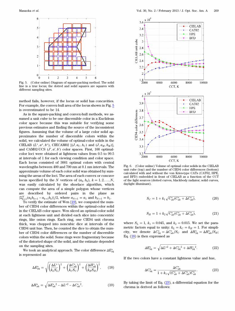
method fails, however, if the locus or solid has concavities.For example, the convex-hull area of the locus shown in Fig. 5is overestimated to be 14.

As in the square-packing and convex-hull methods, we as-sumed a unit cube to be one discernible color in a Euclideancolor space because this was suitable for verifying someprevious estimates and finding the source of the inconsistentfigures. Assuming that the volume of a large color solid ap-proximates the number of discernible colors within thesolid, we calculated the volume of optimal-color solids in theCIELAB �L�; a�; b��, CIECAM02 [�J; aC; bC� and �J; aM; bM�],and CAM02-UCS �J 0; a0; b0� color spaces. First, 100 optimal-color loci were obtained at lightness values from 0.5 to 99.5at intervals of 1 for each viewing condition and color space.Each locus consisted of 3001 optimal colors with centralwavelengths between 400 and 700 nm at 0.1 nm intervals. Theapproximate volume of each color solid was obtained by sum-ming the areas of the loci. The area of each convex or concavelocus specified by the N vertices of �ak; bk�, k � 1; 2;…; N ,was easily calculated by the shoelace algorithm, whichcan compute the area of a simple polygon whose verticesare described by ordered pairs in the plane asjΣN

k�1�akbk�1 − ak�1bk�j∕2, where aN�1 � a1 and bN�1 � b1.To verify the estimate of Wen [19], we computed the num-

ber of CIE94 color differences within the optimal-color solidin the CIELAB color space. Wen sliced an optimal-color solidat each lightness unit and divided each slice into concentricrings, like onion rings. Each ring, one CIE94 unit chromathick, was chopped into noncubic dice at intervals of theCIE94 unit hue. Then, he counted the dice to obtain the num-ber of CIE94 color differences or the number of discerniblecolors within the solid. Some rings were fragmentary becauseof the distorted shape of the solid, and the estimate dependedon the sampling sites.

We took an analytical approach. The color difference ΔE�94

is represented as

ΔE�94 �

��ΔL�

kLSL

�2�

�ΔC�

ab

kCSC

�2�

�ΔH�

ab

kHSH

�2

s; (18)

ΔH�ab �

��ΔE�

ab2− ΔL�2

− ΔC�ab

2q

; (19)

SC � 1� k1��C�

ab�C�ab � ΔC�

ab�p

; (20)

SH � 1� k2��C�

ab�C�ab � ΔC�

ab�p

; (21)

where SL � 1, k1 � 0.045, and k2 � 0.015. We set the para-metric factors equal to unity: kL � kC � kH � 1. For simpli-city, we denote ΔC�

94 � ΔC�ab∕SC and ΔH�

94 � ΔH�ab∕SH ;

Eq. (18) is then expressed as

ΔE�94 �

��ΔL�2 � ΔC�

942 � ΔH�

942

q: (22)

If the two colors have a constant lightness value and hue,

ΔC�94 �

ΔC�ab

1� k1��C�

ab � ΔC�ab�C�

ab

p : (23)

By taking the limit of Eq. (23), a differential equation for thechroma is derived as follows:

Fig. 5. (Color online) Diagram of square-packing method. The solidline is a true locus; the dotted and solid squares are squares withdifferent sampling sites.

Fig. 6. (Color online) Volume of optimal color solids in the CIELABunit cube (top) and the number of CIE94 color differences (bottom)calculated with and without the von Kries-type CATs (CAT02, HPE,and BFD) embedded in front of CIELAB as a function of the CCTof the light sources (dotted curves, blackbody radiator; solid curves,daylight illuminant).


dC�94

dC�ab

� limΔC�

ab→0

ΔC�94

ΔC�ab

� 11� k1C�

ab: (24)

Next, consider that the two colors have a constant chroma ofC�

ab∕ cos�Δhab∕2�, at the midpoint of which is C�ab, and a con-

stant lightness value. When jΔhabj ≪ 1,

ΔH�ab � 2C�

ab tan�Δhab∕2� ≈ C�abΔhab: (25)

Then ΔH94 is approximated as

ΔH�94 ≈

C�abΔhab

1� k2C�ab: (26)

Consider an isosceles triangle whose base is ΔH�94 and height

is C�ab; when its apex is positioned at the achromatic point

�a� � b� � 0�, the number of CIE94 color differences ΔA�94

within the triangle is approximately

ΔA�94 �

ZC�ab

0ΔH94dC�

94 ≈

ZC�ab

0

C�abΔhab

1� k2C�ab

dC�ab

1� k1C�ab

� Δhab ·k1 ln�k2C�

ab � 1� − k2 ln�k1C�ab � 1�

k1k2�k1 − k2�. (27)

Given that the nth optimal color of N points enclosing a two-dimensional area has a hue difference Δhab�n� and chromaC�

ab�n�, Δhab�n� � �hab�n − 1� − hab�n� 1��∕2. Note thatΔhab�n� may be negative. The number of CIE94 color differ-ences in the area enclosed by a locus consisting of N optimalcolors is calculated as ΣN

n�1ΔA�94�n�, where hab�0� � hab�N�

and hab�N � 1� � hab�1�. The total number of CIE94 colordifferences within an optimal-color solid is calculated by sum-ming the number of CIE94 color differences within 100 lociobtained in the CIELAB color space.

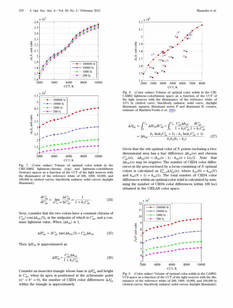
Fig. 7. (Color online) Volume of optimal color solids in theCIECAM02 lightness–chroma (top) and lightness–colorfulness(bottom) spaces as a function of the CCT of the light sources withthe illuminance of the reference white of 200, 1000, 10,000, and100,000 lx (dotted curves, blackbody radiator; solid curves, daylightilluminant).

Fig. 8. (Color online) Volume of optimal color solids in the CIE-CAM02 lightness–colorfulness space as a function of the CCT ofthe light sources with the illuminance of the reference white of1571 lx (dotted curve, blackbody radiator; solid curve, daylightilluminant; squares, illuminant series F and illuminant E; crosses,estimate of Martínez-Verdú et al. [20]).

Fig. 9. (Color online) Volume of optimal color solids in the CAM02-UCS space as a function of the CCT of the light sources with the illu-minance of the reference white of 200, 1000, 10,000, and 100,000 lx(dotted curves, blackbody radiator; solid curves, daylight illuminant).


3. RESULTSA. CIELAB-Based AnalysisFigure 6 shows the volume of optimal-color solids in theCIELAB color space (top) and the number of CIE94 colordifferences (bottom) as a function of the CCT of the lightsources, which consisted of blackbody radiators (2000–4000 K) and daylight illuminants (4000–10,000 K). The vo-lumes were calculated with and without the von Kries-type

CATs (CAT02, HPE, and BFD) embedded in front of CIELAB.The results clearly show that the number of discernible colorsand the variation with the CCT of the adaptation light sourcedepend on the color model used. The breaks in the curves at4000 K are due to the switch from the spectral power distribu-tion of the blackbody radiator to that of the daylight illumi-nant. The estimated number of colors at a CCT of 6500 Kis 2,286,919 in the CIELAB unit cube, which is close to Pointer

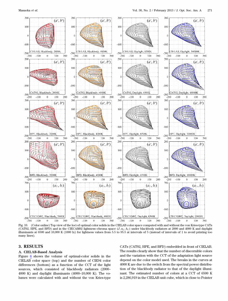
Fig. 10. (Color online) Top view of the loci of optimal color solids in the CIELAB color space computed with and without the von Kries-type CATs(CAT02, HPE, and BFD) and in the CIECAM02 lightness–chroma space �J; aC; bC� under blackbody radiators at 2000 and 4000 K and daylightilluminants at 6500 and 10,000 K (1000 lx) for lightness values from 5.5 to 95.5 at intervals of 5 (instead of intervals of 1 to avoid printing toomany lines).


and Attridge’s [18] estimate of 2.28 million, and the number ofCIE94 color differences is 351,791, which is close to Wen’s[19] estimate of 352,263. These estimates are very sensitiveto the limen chosen [38]. Considering that one JND corre-sponds to half of the CIE94 unit, the estimate for the numberof discernible colors should be larger than the number ofCIE94 color differences by a factor of eight. At 6500 K, thevolume is estimated to be 2,110,746, which is again close toPointer and Attridge’s estimate.

B. CIECAM02-Based AnalysisFigure 7 shows the volume of optimal-color solids in theCIECAM02 �J; aC; bC� and �J; aM; bM� spaces as a function ofthe CCT for Ew values of 200, 1000, 10,000, and 100,000 lx.Morovic et al.’s [23] estimate of 3.8 million JaCbC cubes underilluminant D50 with an Ew of about 1000 lx is considerablylarger than our estimate of 2,078,589, although our result isslightly larger than Morovic’s previous estimate of 1.9 millionin his book [22], despite his use of the convex-hull method.The former discrepancy is due to miscalculation on their part;the latter is due to the somewhat sparse sampling of optimalcolors in his computation [39]. Figure 8 shows the results ofMartínez-Verdú et al. [20] and our estimate for an Ew value of1571 lux (LA � 100). These results are similar, although theirhighest number under illuminant E does not match ours.Figure 9 shows the volume of optimal-color solids in theCAM02-UCS �J 0; a0; b0� space as a function of the CCT for Ew

values of 200, 1000, 10,000, and 100,000 lx. The volumeincreases as the CCT and illuminance of the reference whiteincrease, which is the same trend as in Fig. 7 (bottom),although the estimate is relatively small.

4. DISCUSSIONThe tendencies in the estimations are determined mainlyby the CAT. As shown in Fig. 6, the volume estimated usingCIELAB (without the von Kries-type CATs) peaks at around4000 K. The estimates made using CAT02 increase as the CCTincreases, whereas those made using HPE and BFD decrease.The CIECAM02 estimates (Fig. 7) increase as the CCT in-creases, which is reasonable because the CAT02 chromaticadaptation transform is the main component of CIECAM02.On the whole, the estimates of standard illuminants shownin Fig. 8 also increase with the CCT, despite the dependenceon the illuminant spectra. The CAM02-UCS estimates also in-crease with the CCT for the same reason as for the CIECAM02estimates.

Figure 10 shows the top view of the loci of optimal-colorsolids in the CIELAB color space computed with and withoutthe von Kries-type CATs (CAT02, HPE, and BFD) and in theCIECAM02 �J; aC; bC� color space under blackbody radiatorsat 2000 K and 4000 K and daylight illuminants at 6500 K and10,000 K (1000 lx). Figure 11 shows the corresponding hueangular volume. CAT02 and CIECAM02 exhibit essentially thesame trends in the hue angular volume: the yellow componentincreases as the CCT increases, although the shapes of the locidiffer depending on the chromatic adaptation model. Thematrix coefficients of CAT02 in Eq. (4) and BFD in Eq. (6)are relatively close to each other, whereas the shapes of theloci differ. These results indicate that a slight difference in thecoefficients of the CAT matrices produces different trends involume estimation.

As shown in Fig. 7, the estimates in the CIECAM02lightness–chroma space �J; aC; bC� and lightness–colorfulnessspace �J; aM; bM� increase as the CCT increases. However, theformer is approximately independent of the adaptation lumi-nance level, whereas the latter increases with the illuminanceof the reference white Ew. This is reasonable from the rela-tionship between chroma and colorfulness described inEq. (15). When LA ≫ 1, the fourth power of k in Eq. (14) isapproximated as zero, and Eq. (13) is then reducedto FL ≈ 0.1�5LA�1∕3 � 0.1�Ew∕π�1∕3. Then M � 0.79C for Ew

Fig. 11. (Color online) Hue angular volume of optimal color solids inthe CIELAB color space computed with and without the von Kries-type CATs (CAT02, HPE, and BFD) and in the CIECAM02 lightness–chroma space �J; aC; bC� under blackbody radiators at 2000 and4000 K and daylight illuminants at 6500 and 10,000 K (1000 lx).


values of 200 lx, M � 0.91C for 1000 lx, M � 1.10C for10,000 lx, and M � 1.33C for 100,000 lx. The volume ratiosin lightness–colorfulness to lightness–chroma are thenroughly 0.63∶1 for 200 lx, 0.83∶1 for 1000 lx, 1.21∶1 for10,000 lx, and 1.78∶1 for 100,000 lx.

It might be reasonable to use CAM02-UCS rather thanCIECAM02 for the estimation because CIECAM02 was origin-ally designed as a color appearance model, not a uniform

color space in terms of color differences. The significant de-pendence of the volume estimation on the illuminance ofthe reference white is, however, not taken into account. TheCIECAM02 lightness–colorfulness space was selected for thebase color space of CAM02-UCS because its performance fac-tor measure (PF∕3) [40] was slightly better in the lightness–colorfulness space than in the lightness–chroma space.However, the combination of lightness and colorfulness is

Fig. 12. (Color online) Chromaticity distributions of the Munsell matte colors in the CIELAB color space computed with and without the vonKries-type CATs (CAT02, HPE, and BFD) and in the CIECAM02 lightness–chroma space �J; aC; bC� under blackbody radiators at 2000 and 4000 Kand daylight illuminants at 6500 and 10,000 K (1000 lx). The marker color represents the Munsell matte colors simulated under illuminant D65.


unreasonable because lightness is a relative correlate andcolorfulness is an absolute correlate [33]. It seems to be nat-ural in terms of matching the type of scale to use brightness–colorfulness or lightness–chroma, although further study is

needed to determine which color space is reasonable forcomputing the volume of color solids.

Morovic et al. [23] noted that any color appearance modelfails to estimate the number of discernible colors within anoptimal-color solid because the gamut is larger than the psy-chophysical data it is derived from: for CIECAM02, theLUTCHI data [24] were used. CIELAB has a limitation rootedin its development [41]: it was optimized on the basis of theMunsell system, which is defined only for the CIE 1931 stan-dard observer and illuminant C [42]. We used a dataset [43]consisting of the reflectance spectra of 1269 color chips fromthe matte edition of the Munsell Book of Color as a set of col-ors with a smaller gamut. Figure 12 shows the chromaticitydistributions of the Munsell colors in the CIELAB color spacecomputed with and without the von Kries-type CATs (CAT02,HPE, and BFD) and in the CIECAM02 lightness–chroma space�J; aC; bC� under blackbody radiators at 2000 and 4000 K anddaylight illuminants at 6500 and 10,000 K (1000 lx). Figure 13shows the convex-hull volume of the Munsell color solid inthe CIELAB unit cube calculated with and without the vonKries-type CATS (CAT02, HPE, and BFD), as well as in theCIECAM02 JaCbC unit cube, as a function of the CCT ofthe light sources. The tendencies of increasing and decreasingagain depend on the CAT.

If it is assumed that the goal of chromatic adaptation is tomaximize color constancy, the adaptation model with the flat-test curve is probably the best. If instead it is assumed that

Fig. 13. (Color online) Convex-hull volume of Munsell matte colorsin the CIELAB color space calculated with and without the von Kries-type CATs (CAT02, HPE, and BFD) and in the CIECAM02 lightness–chroma space �J; aC; bC� as a function of the CCT of the light sources(1000 lx) (dotted curves, blackbody radiator; solid curves, daylightilluminant).

Fig. 14. (Color online) Chromaticity distributions of the Munsell matte colors in the CIECAM02 lightness–chroma space �J; aC; bC� under black-body radiators at 2000 and 4000 K and daylight illuminants at 6500 and 10,000 K (1000 lx) with D factors of 1 (complete adaptation), 0.8, and 0.6(practical lower limit of incomplete adaptation). The marker color represents the Munsell matte colors simulated under illuminant D65.


chromatic adaptation is about maximizing the number ofperceptible colors overall, then maximizing the area might bebetter (especially at low CCTs and low luminance levels at thebeginning and end of the day), and the model with the max-imum area might be better. It would be prudent to considerthem both to be partial factors. However, it is probably safestto assume that the gamut volume and chromatic adaptationare related only incidentally.

Figure 14 shows the chromaticity distributions of theMunsell colors in the CIECAM02 lightness–chroma space�J; aC; bC� under blackbody radiators at 2000 and 4000 Kand daylight illuminants at 6500 and 10,000 K (1000 lx) withD factors of 1 (complete adaptation), 0.8, and 0.6 (practicallower limit of incomplete adaptation). Figure 15 shows thevolume of the Munsell colors in the CIECAM02 JaCbC unitcube as a function of the CCT of the light sources. The shapesof the curves representing the volume calculated with CAT02in Fig. 13 and CIECAM02 (D � 1) in Fig. 15 resemble eachother. The volume with D � 0.6 and D � 0.8 in CIECAM02,however, increases unrealistically with the CCT, whichindicates a defect in the CAT.

Martínez-Verdú et al. [20] suggested the possibility of analternative color-rendering index based on the number of dis-cernible colors within an optimal-color solid. As shown inFig. 8, however, their highest number under illuminant Edid not match ours because of miscalculation on their part[44]. In either case, the volume estimation depends stronglyon the color appearance model used, and the ranking ismerely an artifact of CIECAM02. Pinto et al. [45,46] conductedsubjective experiments to determine the CCT of daylightillumination preferred by observers when appreciating artpaintings. They computed the chromatic diversity underdaylight illuminants with CCTs of 3600–25,000 K in theCIELAB color space and counted the number of nonemptyunit cubes occupied by the corresponding color volume. Theyfound that the distribution of observers’ preferences had amaximum at a CCT of about 5100 K and suggested that thispreference has a positive correlation with the number ofdiscernible colors. From Figs. 6 and 13, where the volumeestimated with CIELAB peaks at around 4000 K, the matchbetween the preference and the number of discerniblecolors is, however, undeniably coincidental. Masuda andNascimento [47] investigated illuminant spectra maximizingthe theoretical limits of the perceivable object colors. Theycomputed the volume of the optimal-color solid in the CIELABcolor space under a large number of metameric illuminants atCCTs of 2222–20,000 K and identified a maximum volume ataround 5700 K. They suggested that the estimate of Martínez-Verdú et al. that illuminant E (CCT � 5460 K) ranked first ingamut volume, and the positive correlation between a CCT of5100 K and observers’ preferences found by Pinto et al. were,along with their findings, possible grounds for the use of thestandard illuminant D50 in the printing industry. Quintero et al.[48] suggested that colorfulness evaluated on the basis ofthe volume of optimal-color solids complements the generalcolor-rendering index based on color fidelity. However, asdescribed in Section 2, CIELAB has an intrinsic limitationin the applicable range of its adaptation transform, so compar-isons of the volume estimated using CIELAB at different colortemperatures are not reliable.

To solve the conundrum, we must find a non-von Kries-typeCAT or a completely new color appearance model, but that iswell beyond the scope of this paper, or indeed any singlepaper. There are no documents that clearly and correctly de-scribe the applicable range of the von Kries-type chromaticadaptation in terms of color temperature change for this typeof computation. In fact, von Kries had fairly low expectationsof his ideas on chromatic adaptation [35], but his work hasstood up rather well over the past 100 years. Although our re-search shows negative results, we believe it is a significantstep in the advancement of color science.

5. CONCLUSIONSWe estimated the number of discernible colors over a widerange of color temperatures and illuminance levels using sev-eral color models and fast, accurate methods and verified theprevious estimates; some estimates are almost the same asours, and the others are miscalculations on the part of theirauthors. Our comprehensive simulation revealed that the es-timates depend strongly on the color model used. The varia-tions in the volume as a function of the color temperaturewere determined mainly by the CAT, and slight differencesin the coefficients of the CAT matrices caused different trendsin the estimation. The applicable range of the von Kries-typechromatic adaptation is unknown in terms of the color tem-perature change for this type of computation. In particular, theD factor or degree of adaptation incorporated in the CAT ma-trices has an unnatural effect on the estimate. In addition, thechoice between the absolute correlate and the relative corre-late significantly affects the dependence of the volume estima-tion on the illuminance level. As far as the ranking of thenumber of discernible colors is concerned, further researchis required to compare the estimates at different color tem-peratures and illuminance levels, even if the gamut is small.Thus, the number of discernible object colors remains aconundrum.

Fig. 15. (Color online) Convex-hull volume of Munsell matte colorsin the CIECAM02 lightness–chroma space �J; aC; bC�with D factors of1 (complete adaptation), 0.8, and 0.6 (practical lower limit of incom-plete adaptation) as a function of the CCT of the light sources(1000 lx) (dotted curves, blackbody radiator; solid curves, daylightilluminant).


APPENDIX A: MATLAB CODE FORCOMPUTING OPTIMAL COLORS WITH ACOLOR APPEARANCE MODEL

function Lab � optimalcolor locus �Lc; cmf;S�% Lc: constant lightness value% cmf: color-matching functions (N × 3)% S: illuminant spectrum (N × 1)T � cmf: � repmat�S�:�; �1 3��;T � T:∕sum�T�:; 2�� 100;XYZws � sum�T�;N � length�T�;T � repmat�T; �3 1��; % concatenationtol � optimset�‘MaxIter’; ‘Inf ’; ‘TolFun’; 1e − 10�;for n � 1∶Nfval � inf;while fval > 1e − 7‖h > N∕2‖h < 0

�h fval� � fminsearch�@�x�…abs�Lc-optc�T;n� N; x;XYZws��;N∕2 � rand; tol�;

end�∼; Lab�n; :�� optc�T; n� N;h;XYZws�;

end

function �LLab� � optc�T;n; h;XYZws�b � n − floor�h�: n� floor�h�; % bodym � h − floor�h�; % marginif ∼isempty�b�Lab � �T�b�1� − 1; :� �m� T�b�1�; :� � �2 −m�� m∕2…

��T�b�end� � 1; :� �m� T�b�end�; :� � �2 −m�� m∕2…�sum�T�b; :�; 1� − T�b�1�; :�∕2 − T�b�end�; :�∕2;

Lab � your color appearance model�Lab;XYZws�;L � Lab�1�;

elseL � inf;

end

REFERENCES1. J. Morovic, P. L. Sun, and P. Morovic, “The gamuts of input

and output colour imaging media,” Proc. SPIE 4300, 114–125(2001).

2. R. G. Kuehni, Color Space and its Divisions: Color Order from

Antiquity to the Present (Wiley, 2003), pp. 202–203.3. E. B. Titchener, Outline of Psychology (Macmillan, 1896), p. 48.4. E. B. Titchener, Outline of Psychology: New Edition with

Additions (Macmillan, 1899), p. 55.5. E. G. Boring, H. S. Langfeld, and H. P. Weld, Introduction to

Psychology (Wiley, 1939), p. 517.6. D. B. Judd and K. L. Kelly, “Method of designating colors,” J. Res.

Nat. Bur. Stand. 23, 355–366 (1939).7. D. B. Judd and G. Wyszecki, Color in Business, Science, and

Industry, 3rd ed. (Wiley, 1975).8. R. M. Halsey and A. Chapanis, “On the number of absolutely

identifiable spectral hues,” J. Opt. Soc. Am. 41, 1057–1058(1951).

9. A. Hård and L. Sivik, “NCS–natural color system: aSwedish standard for color notation,” Color Res. Appl. 6,129–138 (1981).

10. W. Ostwald, “Neue Forschungen zur Farbenlehre,” Phys. Z. 17,322–332 (1916).

11. E. Schrödinger, “Theorie der Pigmente von größterLeuchtkraft,” Ann. Phys. 367, 603–622 (1920).

12. R. Luther, “Aus demGebiete der Farbreiz-Metrik,” Z. Tech. Phys.8, 540–558 (1927).

13. N. D. Nyberg, “Zum Aufbau des Farbkörpers im Raume allerLichtempfindungen,” Z. Phys. 52, 406–419 (1929).

14. S. Rösch, “Die Kennzeichnung der Farben,” Z. Phys. 29, 83–91(1928).

15. D. L. MacAdam, “The theory of maximum visual efficiencyof colored materials,” J. Opt. Soc. Am. 25, 249–252(1935).

16. D. L. MacAdam, “Maximum visual efficiency of colored materi-als,” J. Opt. Soc. Am. 25, 361–367 (1935).

17. D. Nickerson and S. M. Newhall, “A psychological color solid,”J. Opt. Soc. Am. 33, 419–422 (1943).

18. M. R. Pointer and G. G. Attridge, “The number of discerniblecolours,” Color Res. Appl. 23, 52–54 (1998).

19. S. Wen, “A method for selecting display primaries tomatch a target color gamut,” J. Soc. Inf. Disp. 15, 1015–1022(2007).

20. F. Martínez-Verdú, E. Perales, E. Chorro, D. de Fez, V. Viqueira,and E. Gilabert, “Computation and visualization of theMacAdam limits for any lightness, hue angle, and light source,”J. Opt. Soc. Am. A 24, 1501–1515 (2007).

21. “A colour appearance model for colour management systems:CIECAM02,” CIE 159:2004 (CIE, 2004).

22. J. Morovic, Color Gamut Mapping, 1st ed. (Wiley, 2008),p. 161.

23. J. Morovic, V. Cheung, and P. Morovic, “Why we don’t knowhow many colors there are,” in Proceedings of IS&T CGIV

2012: Sixth European Conference on Colour in Graphics, Ima-

ging, and Vision (Society for Imaging Science and Technology,2012), pp. 49–53.

24. M. R. Luo, A. A. Clarke, P. A. Rhodes, A. Schappo, S. A. R.Scrivener, and C. J. Tait, “Quantifying colour appearance. Part I.LUTCHI colour appearance data,” Color Res. Appl. 16, 166–180(1991).

25. M. R. Luo, G. Cui, and C. Li, “Uniform colour spaces basedon CIECAM02 colour appearance model,” Color Res. Appl.31, 320–330 (2006).

26. “Control of damage to museum objects by optical radiation,”CIE 157:2004 (CIE, 2004).

27. “Industrial colour-difference evaluation,” CIE 116:1995 (CIE,1995).

28. K. Masaoka, “Fast and accurate model for optimal colorcomputation,” Opt. Lett. 35, 2031–2033 (2010).

29. G. Wyszecki and W. S. Stiles, Color Science: Concepts and

Methods, Quantitative Data and Formulae (Wiley, 2000).30. “Recommended practice for tabulating spectral data for use in

colour computations,” CIE 167:2005 (CIE, 2005).31. C. Li, M. R. Luo, M. S. Cho, and J. S. Kim, “Linear programming

method for computing the gamut of object color solid,” J. Opt.Soc. Am. A 27, 985–991 (2010).

32. M. D. Fairchild, “Testing colour-appearance models: Guidelinesfor coordinated research,” Color Res. Appl. 20, 262–267(1995).

33. M. D. Fairchild, Color Appearance Models, 2nd ed. (Wiley, 2005).34. “Colorimetry,” CIE 15.3:2004 (CIE, 2004).35. J. von Kries, Chromatic Adaptation, Festschrift der Albercht-

Ludwig-Universität (Fribourg, 1902).36. P. Green, Color Management: Understanding and Using ICC

Profiles, 1st ed. (Wiley, 2010).37. E. Perales, F. Martínez-Verdú, V. Viqueira, M. J. Luque, and P.

Capilla, “Computing the number of distinguishable colors underseveral illuminants and light sources,” in Proceedings of IS&T

CGIV 2006: Third European Conference on Colour in

Graphics, Imaging, and Vision (Society for Imaging Scienceand Technology, 2006), pp. 414–419.

38. C. S. McCamy, “On the number of discernible colors,” Color Res.Appl. 23, 337 (1998).

39. J. Morovic, Hewlett-Packard Ltd., 42 Scythe Way, Colchester,CO3 4SJ, UK (personal communication, 2012).

40. C. Li, M. R. Luo, and G. Cui, “Colour-differences evaluation usingcolour appearance models,” in Proceedings of IS&T/SID CIC11:

Eleventh Color Imaging Conference (Society for ImagingScience and Technology, 2003), pp. 127–131.

41. R. S. Berns, Billmeyer and Saltzman’s Principles of

Color Technology, 3rd ed. (Wiley-Interscience, 2000),pp. 68–69.

42. S. M. Newhall, D. Nickerson, and D. B. Judd, “Final report ofthe O.S.A. subcommittee on the spacing of the Munsell colors,”J. Opt. Soc. Am. 33, 385–418 (1943).

43. University of Eastern Finland, Spectral Image Database, http://spectral.joensuu.fi/.

44. E. Perales, Department of Optics, Pharmacology andAnatomy, University of Alicante, Carretera de San Vicente del


http://spectral.joensuu.fi/




Raspeig s/n 03690, Alicante, Spain (personal communication,2012).

45. P. D. Pinto, J. M. Linhares, J. A. Carvalhal, and S. M. Nascimento,“Psychophysical estimation of the best illumination for apprecia-tion of Renaissance paintings,” Vis. Neurosci. 23, 669–674 (2006).

46. P. D. Pinto, J. M. Linhares, and S. M. Nascimento, “Correlatedcolor temperature preferred by observers for illumination

of artistic paintings,” J. Opt. Soc. Am. A 25, 623–630(2008).

47. O. Masuda and S. M. Nascimento, “Lighting spectrum to maxi-mize colorfulness,” Opt. Lett. 37, 407–409 (2012).

48. J. M. Quintero, C. E. Hunt, and J. Carreras, “De-entangling color-fulness and fidelity for a complete statistical description of colorquality,” Opt. Lett. 37, 4997–4999 (2012).


Number of discernible object colors is a conundrumrit-mcsl.org/fairchild//PDFs/PAP32.pdf · Number...

Documents

Transcript of Number of discernible object colors is a conundrumrit-mcsl.org/fairchild//PDFs/PAP32.pdf · Number...