NUCLEAR MAGNETIC RESONANCE - Physics...

Physics 122 Lab NMR Experiment

File – NMR Manual_1/22/08.doc Brian Barnett 1/22/08 of 26

Continuous Nuclear Magnetic Resonance

Physics 122 Lab



Contents

Introduction Page 3, 4

Experiment

General Experiment Page 5

Function of System Components Page 6 - 13

Basic Procedure Page 14, 15

Running the Experiment Page 16 - 23

Appendix

References Page 26

Textbooks Page 26



NUCLEAR MAGNETIC RESONANCE

Introduction:

For the purposes of this experiment, the nuclei of a collection of atoms may be regarded in lowest approximation as an assembly of non-interacting magnetic moments in a magnetic field. The Hamiltonian for a single nuclear magnetic moment in a magnetic field is

(1)

where is the angular momentum of the nucleus; , the magnetic field present at the nucleus; g, the nuclear Land’e g-factor, and µN, the nuclear magneton.

(2)

This equation is in cgs units, as are all the subsequent equations in the writeup of this experiment. Note that when people refer to the “magnetic moment in nuclear magnetons”, they mean the product, gI.

Assuming a magnetic field present along the z-axis of magnitude Hz, the expectation values of H are

(3)

The energy levels are then of the following form.

For the case I=½. The transition indicated by the arrow has the frequency

ν0=gµNHZ / h (4)

for all values of I since the selection rule is �mI=1. For the proton this transition is at

4.2576 kHz / gauss. Note that this energy separation can also be described using angular frequency ω0 = 2πνo.

HIH •μg N=

I H

mcNhμ e

2=

H zI HmgEnergy = ⟨ Nμ=⟩

mI=-1/2

mI=1/2

Energy

Hz



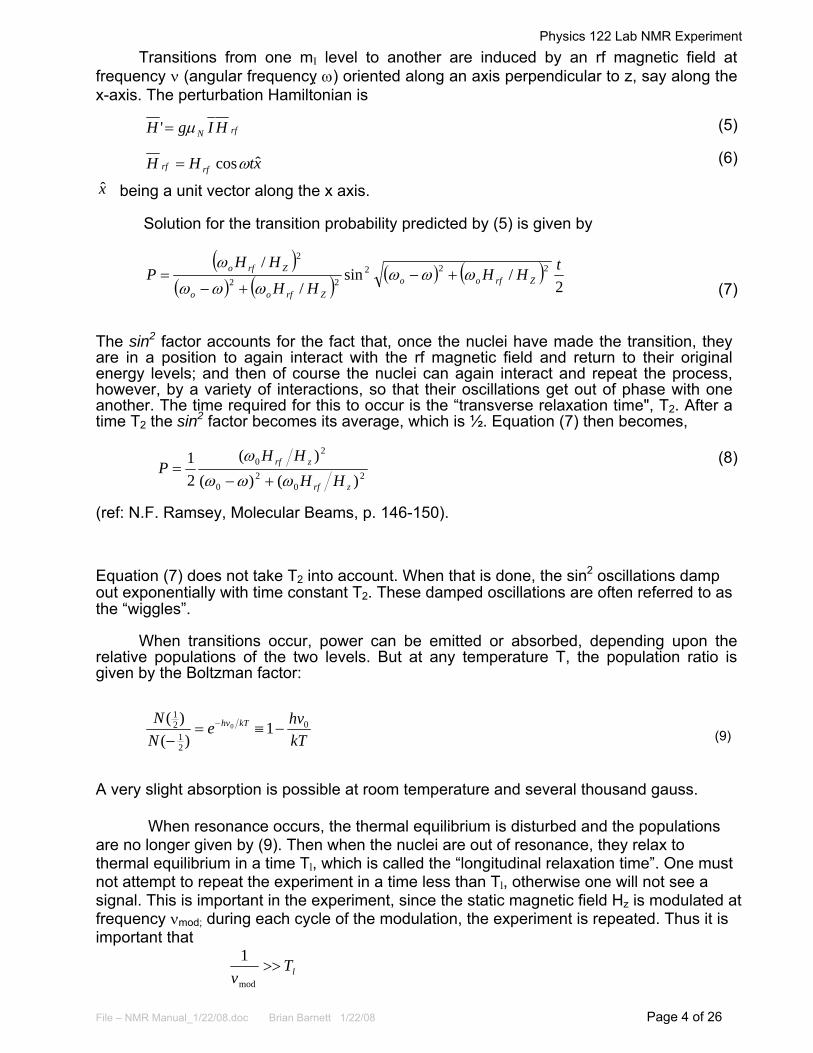
Transitions from one mI level to another are induced by an rf magnetic field at frequency ν (angular frequency ω) oriented along an axis perpendicular to z, say along the x-axis. The perturbation Hamiltonian is

(5) rfN HIgH μ='

(6) xtHH rfrf ˆcosω=

x being a unit vector along the x axis.

Solution for the transition probability predicted by (5) is given by

( )( ) ( ) ( ) ( )

2/sin

/

/ 22222

2tHH

HH

HHP Zrfoo

Zrfoo

Zrfo ωωωωωω

ω+−

+−=

(7)

The sin2 factor accounts for the fact that, once the nuclei have made the transition, they are in a position to again interact with the rf magnetic field and return to their original energy levels; and then of course the nuclei can again interact and repeat the process, however, by a variety of interactions, so that their oscillations get out of phase with one another. The time required for this to occur is the “transverse relaxation time", T2. After a time T2 the sin2 factor becomes its average, which is ½. Equation (7) then becomes,

(8) 2

02

0

20

)()()(

21

zrf

zrf

HHHH

Pωωω

ω+−

= (ref: N.F. Ramsey, Molecular Beams, p. 146-150).

Equation (7) does not take T2 into account. When that is done, the sin2 oscillations damp out exponentially with time constant T2. These damped oscillations are often referred to as the “wiggles”.

When transitions occur, power can be emitted or absorbed, depending upon the

relative populations of the two levels. But at any temperature T, the population ratio is given by the Boltzman factor:

(9) kTN0

10 −

hveN kThv

2

21

1)(

)(≡=

−−

A very slight absorption is possible at room temperature and several thousand gauss.

When resonance occurs, the thermal equilibrium is disturbed and the populations are no longer given by (9). Then when the nuclei are out of resonance, they relax to thermal equilibrium in a time Tl, which is called the “longitudinal relaxation time”. One must not attempt to repeat the experiment in a time less than Tl, otherwise one will not see a signal. This is important in the experiment, since the static magnetic field Hz is modulated at frequency νmod; during each cycle of the modulation, the experiment is repeated. Thus it is important that

lTv

>>mod

1



General Experiment

It is the purpose of this experiment to observe the phenomenon of nuclear magnetic resonance (or "NMR”) and to gain some familiarity with the instrumentation used for its observation.

The NMR is observed by measuring the corresponding change in quality- factor, or

“Q”, of a coil containing a sample. This coil together with a capacitor constitute the tank circuit of a radio frequency oscillator which operates at very low oscillation levels and hence in the extreme non-linear portion of its characteristic. Small changes in Q of the tank circuit result in relatively large changes in oscillation level. It is these changes in oscillation level, after demodulation, that we observe as the NMR signal.

The sample to be tested is placed between the poles of a Varian DC magnet

capable of up to a 9 kiloGauss field. On the inside of the large dc magnet poles are placed coils that are driven at an audio frequency to provide a slowly sweeping AC field at a small fraction of the DC field strength. As the combination of the DC and varying AC field sweep through the NMR range, a signal is produced on the oscilloscope screen. The block diagram below shows the basic system components. A large DC power supply capable of 1500V at up to 1.5 amps supplies regulated power to the large magnet. An audio oscillator provides a continuous audio sine wave to a power amplifier that provides AC power to the relatively small coils between the large magnet poles, and to a phase shifter to synchronize a horizontal sweep signal for the oscilloscopes horizontal deflection amplifier. The amplitude modulated signal from the RF oscillator is fed to a frequency counter to provide an accurate frequency measurement and to an AM detector to provide a demodulated signal for the oscilloscopes vertical deflection amplifier.

RFOscillator

FrequencyCounter

Detector

Oscilloscope

Vert HorizPhase Shifter

AudioPower Amp

AudioOscillator

Sample

GaussMeter

DC Coil

AC Coil

Probe

DC MagnetPower Supply

NMR Basic Block Diagram



Function of components:

a. RF Oscillator - The oscillator in use is a conventional marginal oscillator. The basic circuit is that of

Proffitt and Gardiner - "Instructional NMR Instrument' Journ. Chem. Educ. 4.1 152 (1966)

This is a standard rf oscillator at the frequency ν which furnishes a linearly polarized rf magnetic field perpendicular to H0 and of magnitude Hrf cos ωt Note that there are now three magnetic fields present: the large DC field H0, plus a time dependent modulation Hmodcos ωmodt both along , as well as the rf field perpendicular to these two. z

The oscillator can be modeled as a series RLC circuit, where L is the inductance of

the rf coil around the sample and C is the capacitance of the tuning capacitors in the oscillator. R is a series resistance present to account for all power losses in the RLC circuit including the effect of the nuclear magnetic resonance. As any beginning physics text shows, the impedance of the circuit at resonance is equal to R and the “quality factor”, Q, (defined as the energy stored in the circuit divided by the energy lost per cycle) is ωL/R, where ω is 2π times the oscillation frequency. As a consequence, at resonance, the impedance of the circuit is proportional to L/Q. (see for example, ED. M Purcell, Electricity and Magnetism, 1969, p. 278.)

When connected as a oscillator, the voltage level of the oscillations is proportional to

the impedance of the circuit, and so to L/Q. But Q represents effects of a number of losses: (11)

NMRdielectric QQQQ11

+=11

0

+ Here Q0 describes the losses in the coil itself, Qdielectric describes the losses in the dielectric sample holder and QNMR the losses in the sample itself. In order for the NMR to be observable, Qo and Qdielectric must be very large, so that their reciprocals will be negligible.

When NMR occurs, a macroscopic magnetic moment, M, appears in the sample,

proportional to Hrf.

( )ttHM rfx ωχωχ sin"cos'2 +=

The quantities χ’ and χ” are called the "rf susceptibilities”. One may show that χ” is proportional to 1/QNMR:.

(12) "4'41

"41 πχπχ

πχ=

Q +=

NMR



As the field is swept through resonance at the modulation frequency νmod, the

oscillation level at the rf oscillator per half cycle is like this:

The envelope traces out the resonance absorption curve of the sample determined by χ”. Since the abscissa is H = H0 + Hrfcosωt, the envelope is χ” (H).

As can be seen in the oscilloscope photos below, the actual waveforms look significantly different from the drawing above.

The small change in the magnetic field causes only a small change in the coils value

and a correspondingly small change in the actual signal amplitude. The change is significant, however, and is enough to detect and display. The photos show the 100 Hz magnetic sweep on the lower trace and the rf signal on the upper traces. The left photo shows the rf signal at over 1.0 volt p/p amplitude with only tiny bumps in the signal discernable. Offsetting the trace and zooming in on the top shows a usable signal of about 5 mV in the right photo.


NMR Oscillator- Functions of Controls:

Coil and Sample

Oscillation Level Adjust


Frequency Adjust Demodulated Output Frequency Adjust Demodulated Output

a) Oscillator

a) Oscillator

b) Detector - This is just a rectifier with a time constant long compared to l/νo. and short

compared to 1/νmod. An especially simple form might be

RF Input Demodulated Output



During the negative half cycle the diode is non-conducting. It conducts during the positive half cycle of the input voltage to keep the capacitor C charged. We require

(13) modωω >>

1>>

RC

The output at the detector, over one half cycle of the modulating frequency, is,

(assuming that the conditions of equation (13) are satisfied). This is the vertical signal to the oscilloscope.

Oscilloscope – We can use two ways of generating the horizontal drive for observation

of the signal.

A) Horizontal drive synchronous with modulation.

Vert amp Time Base

Here only the amplifier in the Time Base is used to get the sweep signal to the

horizontal deflection plates using, Display mode of Amplifier, and Triggering mode of

External Source. During one full cycle of the AC portion of the magnetic field, the CRT

beam will be swept across the CRT face in one direction and then back across in the other

direction. Since the waveform peaks will usually not align this way, a phase shifter circuit is

used between the audio sweep signal and scope amplifier to allow adjustment of the

opposite direction sweep timing to align the peaks.



The Phase Shifter box has both a level control and a phase control. The level

control is adjusted to obtain a full horizontal scan on the CRT and the phase control is

adjusted to align the opposite scan waveforms.



The result of non-aligned sweeps is shown on the left, aligned on the right and an

actual correctly aligned scope waveform below.

B) Internal time base triggered by either modulation or the input signal.

The horizontal sweep can be generated by triggering the time base internally

(Display Mode-Time Base, Triggering Source-Internal) using the modulation signal from the

Vertical Amplifier. This technique is helpful if an accurately linear scale is needed on the

scope screen, such as measuring timing of the wiggles.



DC Magnet and Supply

The Varian Regulated DC Magnet and Power Supply are shown below. This supply

can be adjusted to hold the large magnet at a very stable gauss level from near zero to

about 9 kiloGauss.

120 VAC Power Switch

Low Voltage Tube

Filament Power

Time Delay Adjustable

Auto Transformer

(Variac) &

Interlocks

8 Volt Reference

Supply

Current Meter

Series Pass

Regulator Tubes

High Voltage Transformer

Servo Amplifier

Course/Fine Variable Current

Adjustments

Current Shunt

Regulating Range Meter

And Rectifiers

Magnet



Frequency Counter A Hewlett Packard 5328A Frequency Counter monitors the frequency of the RF oscillator to determine the actual frequency of an observed NMR signal. Gauss Meter

The AlphaLabs DC Magnetometer uses a Hall effect probe that is placed between the two magnet poles to measure the DC magnetic flux.

Audio Signal Generator

The Tektronix SG 502 Oscillator plugs into a Tektronix TM Power Supply Mainframe and feeds audio sine waves to the audio power amplifier.

Audio Power Amplifier The power amplifier driving the AC magnet coils is an Altec Lansing stereo amplifier modified for single channel use with input and monitor connections on the front panel.



Basic Procedure Set up the experimental components according to the block diagram on page 5.

Have your instructor check the set-up then try to find a proton resonance. Pure distilled water will not yield an easily observable signal, you will need some paramagnetic ion relaxer. If CuSO4 is used the solution should be a pale blue.

After obtaining a signal, vary the RF oscillation level, audio power level, probe position in the magnet and the paramagnetic ion concentration to obtain the best signal to noise ratio. Now do a field calibration over the range available to you.

Samples containing protons in H2O, glycerol, polyethylene and paraffin as well as several other nuclei are provided. All can be observed using this apparatus. Their gyromagnetic ratios and isotopic abundances are listed below (1Tesla =10 kiloGauss).

Isotope NMR Freq MHz/Tesla Natural Abundance Spin

1H 42.5759 99.9844% 1/2 7Li 16.546 92.57% 3/2 11B 13.660 81.17% 3/2 19F 40.0541 100% 1/2 27Al 11.094 100% 5/2 51V 11.193 100% 7/2

The nuclei below are more difficult to observe; signal to noise ratio is < 5.

Isotope NMR Freq MHz/Tesla Natural Abundance Spin

203Tl 24.332 29.5% 1/2 205Tl 24.570 70.5% 1/2 31P 17.235 100% 1/2

117Sn 15.186 7.61% 1/2 119Sn 15.869 8.58% 1/2 87Rb 13.932 27.2% 3/2

Use care in handling the fluorine, boron, vanadium, phosphorous, and thallium samples; the triflouracetic and phosphoric acids are highly corrosive and thallium is extremely poisonous.

1. Using the Hall effect gauss meter, measure the g factor for the proton in H2O. This is best done by plotting the nuclear resonance frequency as a function of magnetic field over a substantial range, say 5 MHz - 30 MHz. The least-squares slope of the Line will be the g factor. You will be limited to an accuracy of perhaps 0.1% by the accuracy of the gauss meter. However, the magnet power supply is stable to at least one part in 105; thus it should be possible to measure ratios of NMR frequencies for different elements to this precision in a constant magnetic field, by tuning the oscillator frequency to the different resonances.



2. Using the known g factor of the proton (2 x 2.79270 ) measure the nuclear resonance

frequencies for several of the other isotopes listed, and calculate their g factors. Compare with published values. (See CRC Handbook of Chemistry and Physics and note that the g factor times the spin is the “nuclear moment”.)

3. (a) With the scope horizontal sweep set up for synchronous drive (vert amp rather than time base), measure the width of the proton resonance in water or glycerol in gauss. In this configuration, the horizontal deflection of the oscilloscope is proportional to the magnetic field. The easiest way to calibrate the x-axis is to measure the static field (or better, the NNM frequency) at those points where the nuclear magnetic resonance disappears from the oscilloscope screen. For liquids, the intrinsic NMR line width is very narrow, and virtually all of the observed line width is due to nonuniformities in the applied magnetic field over different parts of the sample.

(b) An alternate method of determining the line width is to measure T2, the transverse

relaxation time or "ring down" time characterizing the “wiggles" which follow rapid transit through the nuclear resonance. The nuclear absorption is described by

,

)(1.)(" 2

22

0 TConst

ωωωχ

−+=

hNgμ

γ =Hγω =0

( )ωχ"The envelope of the “wiggles” is given by the Fourier Transform of

( ) ( ) 2"" Ttti edet −∞

∞−

∝= ∫ ωωχχ ω

2

2T

Hγ

=ΔThe full width at half maximum of χ”(ω) is 2/T2 or, in gauss, Find a sample which displays wiggles when the field sweep is adjusted for fast passage (how fast?), through the resonance, and with the scope set up for internal time base, trigger the oscilloscope internally from the field sweep waveform (vertical channel) using its own internal time base. Then plot the log of the wiggle. amplitude versus time to obtain T2. If possible, compare with the line width �H obtained in (a).

4. The fluorine resonance may also be observed in teflon, a solid white plastic (CF2).

Likewise the proton resonance can be seen in solid polyethylene and paraffm. NMR line widths in solids are typically much larger than in liquids (“dipolar broadening"). The dipolar broadening is averaged out in liquids by the tumbling motion of the atoms, which is much more rapid than the nuclear precession rate. See if you can observe this effect in the solid samples provided.



Running the NMR Experiment The Marginal oscillator: (3 MHz < ν 0 < 30 MHz) (1) RF probes:

You have the choice of a high-frequency (larger wire, fewer turns) probe capable of providing RF oscillation frequencies higher than 10 MHz, and a low-frequency (smaller wire, more turns) probe capable of providing RF oscillation frequencies less than 12 MHz. Since the maximum DC magnetic field is limited to 8500 gauss, you need both probes to measure NMR signals from 1H and 19F (the high-frequency probe) and from 7Li, 11B, and 31P (the low-frequency probe).

(2) After attaching the selected RF probe to the oscillator, Insert the desired sample into the probe and position the assembly so that the sample is at the center of the magnet.

(3) Turn on the rack instruments with the switch on the power strip. This will also supply 12.6 volts to the RF Oscillator tube filaments.

(4) Turn on the power supply for oscillator plate voltage; (5) Set the sensitivity for the "Base Level" to “Hi” (6) Set the dial for the "Base Level" to 6 o'clock;



Plate Voltage power supply Synchronizer power supply Oscillator filament power supply

(7) Set the capacitor (frequency) dial on the side of the oscillator box for the desirable

frequency v. The frequency, v. (in unit of MHz) is read with the HP 5328A Frequency Counter set up as shown below.

FUNCTION – FREQ A FREQ RESOLUTION – 10 KHz SAMPLE RATE - mid range DELAY - OFF (fully counter clockwise) LEVEL A - PRESET (fully counter clockwise) SLOPE - + ATTEN - 1 AC DC - AC COM - SEP



DC magnetic field (50 <Bd, < 8500 gauss) Use a piece of masking tape to hold the gauss meter probe on the side of the RF probe,

or a magnet pole, so that the magnetic field BBdc, at the sample can be read as the magnet power is turned on and adjusted. The gauss meter is battery powered and must be turned on separately from the instrument rack power. Set the gauss meter to the 19,999 position. Note: residual magnetism in the magnets iron poles will cause a reading on the gauss meter with magnet power still off.

Gauss Meter Probe

The DC magnet power supply is a serious piece of vacuum tube electronics as can be seen

in the picture below. Care must be taken in its operation to avoid damage to the system. The tubes will not regulate the magnet current properly if the filaments are not at operating temperature, so they must be allowed to warm up prior to applying high voltage, and the high voltage must be turned off before turning the filament supplies off at shut down to avoid destroying tubes or other components. (yes, I have seen this happen)



Magnet Supply

Regulation Range Meter Magnet Current Meter

(Pass Tube Voltage) Course Current Fine Current Select Select Filament Power Voltage Control High Voltage Switch (Variac) Switch



To turn on the magnet: 1. Turn on the water. (The magnet is water cooled) 2. Check to make sure the autotransformer Voltage Control, sometimes referred to by the

trade names variac or powerstat, is in the off position, fully counter clockwise. 3. Turn on the Filament power switch (green light at left will turn on), wait at least one minute for the vacuum tube filaments to warm up. (This power supply uses vacuum tube technology and the tube filaments must be warm before the tubes will operate correctly. In high power circuitry like this the tubes will not control properly when the filaments are not at operating temperature, but they can still conduct power and cause damage.) 4. With the Voltage Control in the off position (counter clockwise), turn on the High Voltage switch (Red Light at right will turn on). Turn up the Voltage Control (clockwise increases power) until the left hand, Regulator Range meter reads in the darkest band. This indicates the correct operating voltage being dropped across the series pass regulator tubes. To the left of the darkest band you will lose magnet current regulation. To the right of the darkest band is another dark band in which regulation will still occur, but this is not an optimum regulating point. To the far right beyond the dark bands the pass tubes will be operating at too high a power level and might be damaged. IN NO CASE SHOULD YOU LET THIS METER GO OFF SCALE ON THE RIGHT 5. Adjust the coarse and fine controls to obtain the desired magnet gauss value, watch the

voltage meter and adjust the autotransformer as needed to see that it stays in the heaviest black band region

6. Adjust the “Voltage Control" slowly up until the indicator of the

"Regulation Range Meter" moves from the far left to the first black band on. the left side of the meter; (Note: this is, the range of -regulation that you should operate the power supply)

7. Adjust the "Coarse Current" first and the “Fine Current” next to set the magnetic field Bdc, to the desired value as determined by the Table on page 12 for gµN/h and the following relation

( ) dcN Bhgv μ=0 You must continue to adjust the "Voltage Control" such that the regulation range indicator remains in the first black band on the left.



AC magnetic field (Bac): (0 < BBac < 25 Gauss) (1) Use a combination of the sine wave generator (Tektronix SG502) and audio power

amplifier to drive the pair of AC coils to produce an oscillating magnetic field BBac as follows;

2) Set the signal generator with

Frequency-. 40 to 270 Hz Amplitude: 0.5 volts RMS

(3) Connect the output of the signal generator to the Audio In connector of the Power Amplifier.

(4) Connect the output at the rear of the audio power amplifier to the AC Magnet coils and the front panel, monitor output, to the input of the phase- shifter.

(5) Set the Audio Power control at 4 on the power amplifier so that the output voltage is roughly 3.5 volts(Note: this produces an oscillating magnetic field Bac with peak-to-peak amplitude of about 14 gauss);

(6) Connect the NMR voltage signal (the output of the marginal oscillator) to the oscilloscope mainframe (Tektronix 7603) vertical amplifier (AM-6565). Set "VOLTS/DIV" to 1.

(7) Connect the output of the phase shifter to the input of the scopes Time Base. (8) Note- the phase-shifter is used to add an adjustable phase to the sinusoidal wave from sweeping the AC magnet, so that the output of the phase-shifter is in synchronization with the oscillating magnetic field Bac. You can only adjust the phase when you have already found the NMR signal from the sample (see the Measurement Procedure below); (9) Set the switch on the phase-shifter to "1 kHz"; (10) Adjust "Level" on the phase-shifter until the signal just fills the oscilloscope screen

along the x-axis (total of 10 divisions).



Measurement procedures: (1) Set the RF Oscillator to the desired frequency and Fine tune BBdc, by adjusting the "Fine

Current" on the DC magnet supply until you observe the NMR signal as shown in the scope waveform on page 11. (Note- since the screen only displays the signal over a range of 25 gauss or less, you should not dial the "fine Current" too fast or you will miss the signal)

(2) Synchronization of the phase-shifter output and Bac

Once a signal is observed, you will typically see two peaks on the screen that move in opposite directions as you change BBdc this indicates that the phase-shifter output is out of sync with the alternating magnetic field BacB ; Adjust the phase dial until the two peaks overlap on the screen, Now the phase-shifter output along the x-axis is exactly proportional to BBac;

(3) Calibration of the x-axis as the magnetic field axis Since the x-axis is proportional to BBac, you can determine the proportionality constant (in unit of gauss/division) by adjusting Bdc, until the two peaks move together to the far left and then to the far right. The proportionality constant is then obtained by dividing the net change ΔB

Bη

Bdc by 10 (the total number of divisions along x-axis) 10dcB BΔ=η

Using this method, you will find that �BBdc, ~ 14 gauss when the audio amplifier output is at about 3.5 volts, or 4 on the Audio Power control knob.

(4) Calibration of the x-axis as the frequency axis" You may convert the x-axis to the frequency axis with a proportionality constant

( ) BNRFRF hggu ημηη LL sin

Determination of the relation V0 = (gµN /h)BBdc and gµN /h for H, F, Li B, P 1 19 7 II 31

(1) Adjust Bdc to move the two NMR signal peaks to the middle of the screen and record Bdc and v0

(2) Repeat the procedure for a series of v0, and Bdc; Measurement of the FWHM of the NMR for 1H, 19F, 7Li, 11B, 31P Measure the Full-Width-at-Half-Maximum (FWHM) of the NMR signal peaks for all five nuclei on the screen (in unit of division) and use to express the result in terms of frequency. ( ) BN hgRF μη = η




File – NMR Manual_1/22/08.doc Brian Barnett 1/22/08 Page 23 of 26

Turning off the system: Turning off the system: (1) First turn down "Voltage Control" (the heavy variac) on the DC magnet power supply to

zero; (2) Then turn off "High Voltage" on the DC magnet power supply; (3) Turn off "Filament" on the DC magnet power supply, (4) Turn off the power strip on the floor supplying power to the instrument rack (5) Turn off the computer; (6) Turn off the cooling water to the DC magnet.



Computer-aided measurement of NMR signals with a LabVIEW program: This lab is equipped with a computer-aided data acquisition system based on the LabVIEW-6i program (National Instruments) on a PC. The program, 'NMR_2002.vi", is placed on the C Drive in the folder "Physicsl22Lab_folder". Such a program enables one to perform (i) signal averaging so that weak NMR signals from 19F, 7Li, IIBI 31P or even other nuclei

can be detected with much better signal-to-noise ratio; (ii) digital signal processing so that the segments of the NMR signal when the magnetic field is ramped up or down can be displayed and analyzed separately; (iii) save the data in text files so that the results can be analyzed and plotted for laboratory

reports. (1) Connect the phase-shifter output to "ACH0" of BNC-2090; (2) Connect the NMR signal to "ACH2" (ACH! Does not work) of BNC-2090; (3) Set the frequency of the function generator to faudio,= 250Hz (4) Open up the program “NMR-2002.vi” on the C Drive in the folder

"Physicsl22Lab_folder"; (5) Set "Sampling Frequency (fs)":,to “50000” (6) Set "Number of data points per waveform (Ns)" to fs/faudio = 200; (7) Set “Number of waveforms to be averaged”; (8) If you only want to see the data with no intention of saving them, do not press "Save the

Data,?" button; If you do want to save the data, press "Save the data ?"; When the data acquisition is completed, a window will pop up for you to enter the file name and to select where you want the file to go. The data file can be open with MS Excel or KaleidaGraph, both are available on the computer. You may also send the data out through Ethernet from this computer.

(9) To analyze the waveform when the magnetic field is ramped up or down, you can slice the required data from the data file using Excel or KaleidaGraph.

A quick sample of a Proton NMR run in Excel is shown on the next page.



Mhz Gauss

4.25 947 5.4 1200 6.3 1400

7.21 1600 8.1 1800

9.01 2000 9.92 2200

10.818 2400 10.93 2426 11.96 2677

13.4 3000 14.75 3300

16.1 3600 17.89 4000 20.13 4500 22.39 5000 23.86 5327 24.64 5500 26.89 6000 29.15 6500 29.24 6674 30.08 6705 31.42 7000 32.99 7346



References: Melissinos, Experiments in Modem Physics, Ch. 7, Sec's 1-4. Pake, Nuclear Magnetic Resonance, Am. Journal of Physics, 8 438,473 (1950). J.H. Miller, Novel Experiments in Physics, publ by AAPT, p. 421 D.J.E. Ingram. Contemporary Physics, 7, 13 (1966). D.J.E. Ingram, Contemporary Physics, 7, 103 (1966). Kittel, Introduction to Solid State Physics, 5th ed., Chap. 16.

Textbooks: E.R Andrew, Nuclear Magnetic Resonance N. Bloembergen, Nuclear Magnetic Relaxation R.T. Schumacher, Magnetic Resonance C.P. Slichter, Principles of Magnetic Resonance A. Abragam, Principles of Nuclear Magnetism N. Ramsey, Molecular Beam N. Ramsey, Nuclear Moments

NUCLEAR MAGNETIC RESONANCE - Physics...

Documents

Transcript of NUCLEAR MAGNETIC RESONANCE - Physics...