Lecture 1: Constant Strain Triangle The triangular elements with different numbers of nodes are used for solving two dimensional solid members. The linear triangular element was the first type of element developed for the finite element analysis of 2D solids. However, it is observed that the linear triangular element is less accurate compared to linear quadrilateral elements. But the triangular element is still a very useful element for its adaptivity to complex geometry. These are used if the geometry of the 2D model is complex in nature. Constant strain triangle (CST) is the simplest element to develop mathematically. In CST, strain inside the element has no variation (Ref. module 3, lecture 2) and hence element size should be small enough to obtain accurate results. As indicated earlier, the displacement is expressed in two orthogonal directions in case of 2D solid elements. Thus the displacement field can be written as

ud

v (5.1.1)

Here, u and v are the displacements parallel to x and y directions respectively. 5.1.1 Element Stiffness Matrix for CST A typical triangular element assumed to represent a subdomain of a plane body under plane stress/strain condition is represented in Fig. 5.1.1. The displacement (u, v) of any point P is represented in terms of nodal displacements

1 1 2 2 3 3

1 1 2 2 3 3

u N u N u N uv N v N v N v= + += + +

(5.1.2)

Where, N1, N2, N3 are the shape functions as described in module 3, lecture 2.

Fig. 5.1.1 Linear triangular element for plane stress/strain

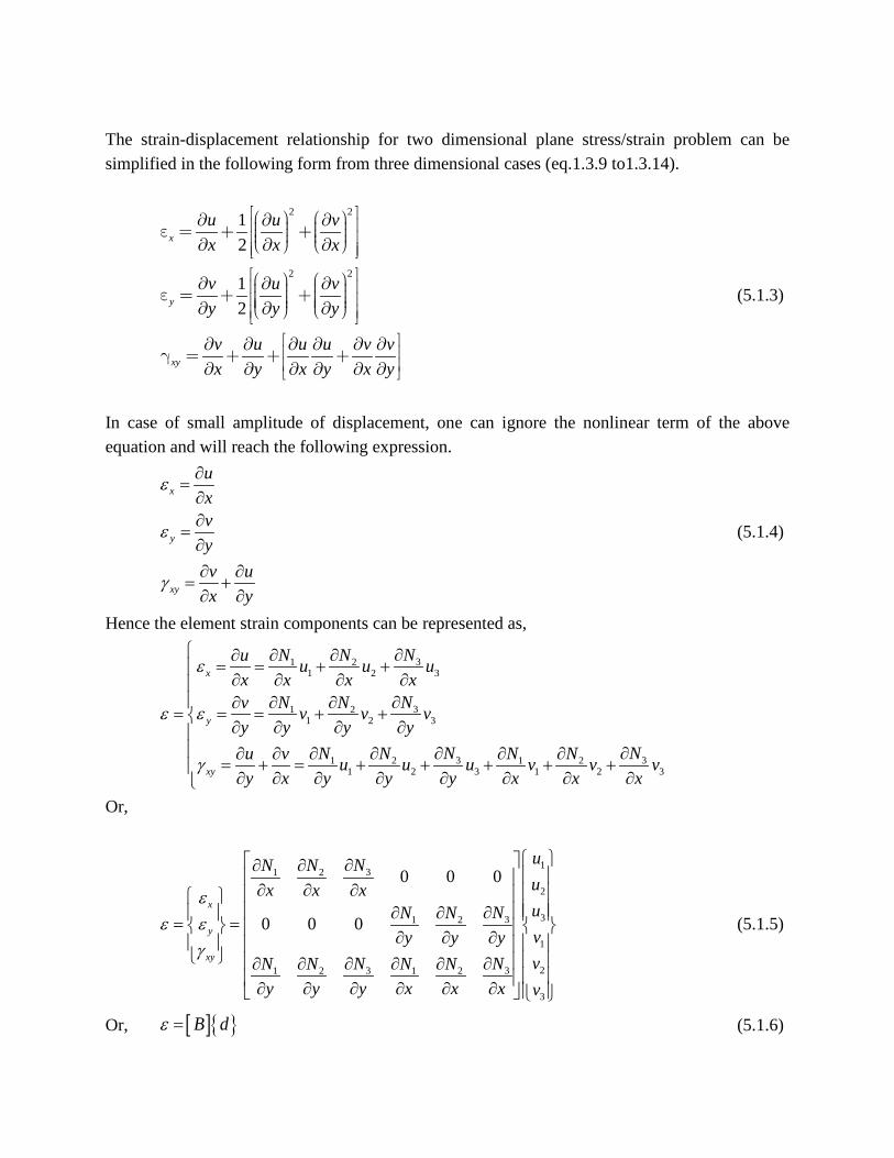
The strain-displacement relationship for two dimensional plane stress/strain problem can be simplified in the following form from three dimensional cases (eq.1.3.9 to1.3.14).

2 2

2 2

12

12

x

y

xy

u u vx x x

v u vy y y

v u u u v vx y x y x y

(5.1.3)

In case of small amplitude of displacement, one can ignore the nonlinear term of the above equation and will reach the following expression.

x

y

xy

uxvyv ux y

ε

ε

γ

∂=∂∂

=∂∂ ∂

= +∂ ∂

(5.1.4)

Hence the element strain components can be represented as,

31 21 2 3

31 21 2 3

3 31 2 1 21 2 3 1 2 3

x

y

xy

NN Nu u u ux x x x

NN Nv v v vy y y y

N NN N N Nu v u u u v v vy x y y y x x x

ε

ε ε

γ

∂∂ ∂∂= = + +∂ ∂ ∂ ∂

∂∂ ∂∂= = = + + ∂ ∂ ∂ ∂ ∂ ∂∂ ∂ ∂ ∂∂ ∂

= + = + + + + +∂ ∂ ∂ ∂ ∂ ∂ ∂ ∂

Or,

131 2

2

331 2

1

23 31 2 1 2

3

0 0 0

0 0 0x

y

xy

uNN Nux x xuNN Nvy y yvN NN N N N

y y y x x x v

εε ε

γ

∂∂ ∂

∂ ∂ ∂ ∂∂ ∂ = = ∂ ∂ ∂

∂ ∂∂ ∂ ∂ ∂ ∂ ∂ ∂ ∂ ∂ ∂

(5.1.5)

Or, [ ] B dε = (5.1.6)

In the above equation [B] is called as strain displacement relationship matrix. The shape functions for the 3 node triangular element in Cartesian coordinate is represented as,

2 3 3 2 2 3 3 2

1

2 3 1 1 3 3 1 1 3

3

1 2 2 1 1 2 2 1

1 x y x y y y x x x y2AN

1N x y x y y y x x x y2A

N 1 x y x y y y x x x y2A

Or,

1 1 1

1

2 2 2 2

3

3 3 3

1 x y2AN1N x y

2AN 1 x y

2A

(5.1.7)

Where,

1 2 3 3 2x y x y , 2 3 1 1 3x y x y , 3 1 2 2 1x y x y ,

1 2 3y y , 2 3 1y y , 3 1 2y y , (5.1.8)

1 3 2x x , 2 2 1x x , 3 2 1x x ,

Hence the required partial derivatives of shape functions are,

1 1 ,2

Nx A

β∂=

∂ 2 2 ,

2Nx A

β∂=

∂ 3 3 ,

2Nx A

β∂=

∂

1 1 ,2

Ny A

γ∂=

∂ 2 2 ,

2Nx A

γ∂=

∂ 3 3 ,

2Nx A

γ∂=

∂

Hence the value of [B] becomes:

[ ]

31 2

31 2

3 31 2 1 2

0 0 0

0 0 0

NN Nx x x

NN NBy y y

N NN N N Ny y y x x x

∂∂ ∂ ∂ ∂ ∂

∂∂ ∂= ∂ ∂ ∂ ∂ ∂∂ ∂ ∂ ∂ ∂ ∂ ∂ ∂ ∂ ∂

Or, [ ]1 2 3

1 2 3

1 2 3 1 2 3

0 0 01 0 0 0

2B

A

β β βγ γ γ

γ γ γ β β β

=

(5.1.9)

According to Variational principle described in module 2, lecture 1, the stiffness matrix is represented as,

[ ] [ ] [ ][ ]Tk B D B dΩ

= Ω∫∫∫ (5.1.10)

Since, [B] and [D] are constant matrices; the above expression can be expressed as

[ ] [ ] [ ][ ] [ ] [ ][ ]T T

V

k B D B d V B D B V= =∫∫∫ (5.1.11)

For a constant thickness (t), the volume of the element will become A.t . Hence the above equation becomes,

[ ] [ ] [ ][ ]Tk B D B At= (5.1.12)

For plane stress condition, [D] matrix will become:

[ ] 2

1 01 0

110 0

2

EDµ

µµ

µ

= − −

(5.1.13)

Therefore, for a plane stress problem, the element stiffness matrix becomes,

[ ] ( )

1 1

2 21 2 3

3 31 2 32

1 11 2 3 1 2 3

2 2

3 3

00

1 0 0 0 00

1 0 0 0 004 1 10 00

20

EtkA

β γβ γ

µ β β ββ γ

µ γ γ γγ βµ

µ γ γ γ β β βγ βγ β

= − −

(5.1.14)

Or,

[ ] ( )

( )

( )

( )

2 21 1 1 2 1 2 1 3 1 3 1 1 1 2 2 1 1 3 3 1

2 22 2 2 3 2 3 2 1 1 2 2 2 2 3 3 2

2 223 3 3 1 1 3 3 2 2 3 3 3

2 21 1 1 2 1 2 1 3 1 3

2 22 2 2 3

12

12

14 1 2

.

C C C C C

C C C CEtk

C C CA

C C CSym C C

µβ γ β β γ γ β β γ γ β γ µβ γ β γ µβ γ β γ

µβ γ β β γ γ µβ γ β γ β γ µβ γ β γ

µβ γ µβ γ β γ µβ γ β γ β γµ

γ β γ γ β β γ γ β βγ β γ γ

++ + + + +

++ + + +

+=+ + +−

+ + ++ + 2 3

2 23 3C

β βγ β

+

(5.1.15)

Where, ( )12

Cµ−

=

Similarly for plane strain condition, [D] matrix is equal to,

[ ] ( )( )

( )( )

1 01 0

1 1 21 20 0

2

EDµ µ

µ µµ µ

µ

−

= − + − −

(5.1.16)

Hence the element stiffness matrix will become:

[ ] ( )

( )( )

2 21 1 1 2 1 2 1 3 1 3 1 1 1 2 2 1 1 3 3 1

2 22 2 2 3 2 3 2 1 1 2 2 2 2 3 3 2

2 23 3 3 1 1 3 3 2 2 3 3 3

2 21 1 1 2 1 2 1 3 1 3

2 22 2 2 3 2 3

3

( 1)1

12 1

.

M M MM M

M CEtkA M M M

Sym M MM

β γ β β γ γ β β γ γ µ β γ µβ γ β γ µβ γ β γβ γ β β γ γ µβ γ β γ µ β γ µβ γ β γ

β γ µβ γ β γ µβ γ β γ µ β γµ γ β γ γ β β γ γ β β

γ β γ γ β βγ

+ + + + + ++ + + + +

+ + + +=

+ + + ++ +

2 23β

+

(5.1.17)

Where ( )1M µ= −

5.1.2 Nodal Load Vector for CST From the principle of virtual work,

T T Td u F d u F d

(5.1.18)

Where, FΓ, and FΩ are the surface and body forces respectively. Using the relationship between stress-stain and strain displacement, one can derive the following expressions:

[ ][ ] [ ] [ ] andD B d , B d u N dσ δ ε δ δ δ= = =

(5.1.19) Hence eq. (5.1.18) can be rewritten as,

TT T T T TSd B D B d d d N F d d N F d

(5.1.20)

Or, TT TSB D B d d N F d N F d

(5.1.21)

Here, [Ns] is the shape function along the boundary where forces are prescribed. Eq.(5.1.21) is equivalent to k d F , and thus, the nodal load vector becomes

T TSF N F d N F d

(5.1.22)

For a constant thickness of the triangular element eq.(5.1.22) can be rewritten as

T TS

S A

F t N F ds t N F dA

(5.1.23)

For the a three node triangular two dimensional element, one can represent Fand F as,

x

y

FF

F

and x

y

FF

F

For example, in case of gravity load on CST element, x

y

F 0F

F g

For this case, the shape functions in terms of area coordinates are:

1 2 3

1 2 3

L L L 0 0 0N

0 0 0 L L L

(5.1.24)

As a result, the force vector on the element considering only gravity load, will become,

1

2

3

1 1 1A A A

2 2 2

3 3 3

L 0 0 0

L 0 0 0

L 0 0 00F t dA t dA dA

0 L L g Lg

0 L L g L

0 L L g L

gt

(5.1.25)

The integration in terms of area coordinate is given by,

1 2 3 22

p q r

A

p! q! r !L L L dA A( p q r )!

=+ + +∫ (5.1.26)

Thus, the nodal load vector will finally become

F

0 00 00 0

1!0!0! gAt2Agt (1 0 0 2)! 3

0!1!0! gAt2A(0 1 0 2)! 3

gAt0!0!1! 2A3(0 0 1 2)!

000gAt1311

(5.1.27)

Lecture 2: Linear Strain Triangle 5.2.1 Element Stiffness Matrix for LST In case of CST, it is observed that the strain within the element remains constant. Though, these elements are able to provide enough information about displacement pattern of the element, but it is unable to provide adequate information about stress inside an element. This limitation will be significant enough in regions of high strain gradients. The use of a higher order triangular element called Linear Strain Triangle (LST) significantly improves the results at these areas as the strin inside the element is varying. The LST element has six nodes (Fig. 5.2.1) and hence, twelve degrees of freedom. Thus the displacement function can be chosen as follows.

2 20 1 2 3 4 5

2 26 7 8 9 10 11

u x y x xy yv a a x a y a x a xy a y

α α α α α α= + + + + +

= + + + + + (5.2.1)

Fig. 5.2.1 Linear strain triangle element

Therefore, the element strain matrix is obtained as

x 1 3 4

y 8 10 11

xy 2 7 4 9 5 10

u 2 x yxv x 2 yyv u ( ) ( 2 )x (2 )yx y

(5.2.2)

In the area coordinate system as discussed in module 3, lecture 3 we can write the shape function for the six node triangular element as

1 1 1 2 2 2 3 3 3

4 1 2 5 2 3 6 3 1

N L 2L 1 N L 2L 1 N L 2L 1N 4L L N 4L L N 4L L

(5.2.3)

The displacement (u,v) of any point within the element can be represented in terms of their nodal displacements with the use of interpolation function.

6

16

1

i ii

i ii

u N u

v N v

=

=

=

=

∑

∑ (5.2.4)

Using eq.(5.2.4) we can rewrite eq.(5.2.2) as,

1

2

3

43 5 61 2 4

5

63 5 61 2 4

1

23 5 6 3 5 61 2 4 1 2 4

3

4

5

6

0 0 0 0 0 0

0 0 0 0 0 0

uuuuN N NN N Nux x x x x xuN N NN N Nvy y y y y yvN N N N N NN N N N N N

y y y y y y x x x x x x vvvv

ε

∂ ∂ ∂∂ ∂ ∂ ∂ ∂ ∂ ∂ ∂ ∂ ∂ ∂ ∂∂ ∂ ∂ = ∂ ∂ ∂ ∂ ∂ ∂

∂ ∂ ∂ ∂ ∂ ∂∂ ∂ ∂ ∂ ∂ ∂ ∂ ∂ ∂ ∂ ∂ ∂ ∂ ∂ ∂ ∂ ∂ ∂

Or, [ ] B dε = (5.2.5)

Where,

[ ]

3 5 61 2 4

3 5 61 2 4

3 5 6 3 5 61 2 4 1 2 4

0 0 0 0 0 0

0 0 0 0 0 0

N N NN N Nx x x x x x

N N NN N NBy y y y y y

N N N N N NN N N N N Ny y y y y y x x x x x x

∂ ∂ ∂∂ ∂ ∂ ∂ ∂ ∂ ∂ ∂ ∂

∂ ∂ ∂∂ ∂ ∂= ∂ ∂ ∂ ∂ ∂ ∂ ∂ ∂ ∂ ∂ ∂ ∂∂ ∂ ∂ ∂ ∂ ∂ ∂ ∂ ∂ ∂ ∂ ∂ ∂ ∂ ∂ ∂ ∂ ∂

(5.2.6)

Using Chain rule,

31 1 1 1 2 1

1 2 3

. . . LN N L N L Nx L x L x L x

∂∂ ∂ ∂ ∂ ∂ ∂= + +

∂ ∂ ∂ ∂ ∂ ∂ ∂

As discussed in module 3, lecture 1, we can write the above expression as,

31 1 1 2 1 1

1 2 3

. . .2 2 2

bN b N b N Nx A L A L A L

∂ ∂ ∂ ∂= + +

∂ ∂ ∂ ∂

( )1 11. 4 1

2N b Lx A

∂= −

∂

Similarly we can evaluate expressions for other terms and can be written as,

( ) ( ) ( )

( ) ( ) ( )

3 31 1 2 21 2 3

5 642 1 1 2 3 2 2 3 1 3 3 1

. 4 1 . 4 1 . 4 12 2 2

4 4 4

N bN b N bL L Lx A x A x A

N NN L b L b L b L b L b L bx x x

∂∂ ∂= − = − = −

∂ ∂ ∂∂ ∂∂

= + = + = +∂ ∂ ∂

And,

( ) ( ) ( )

( ) ( ) ( )

3 31 1 2 21 2 3

5 642 1 1 2 3 2 2 3 1 3 3 1

. 4 1 . 4 1 . 4 12 2 2

4 4 4

N aN a N aL L Ly A y A y A

N NN L a L a L a L a L a L ay y y

∂∂ ∂= − = − = −

∂ ∂ ∂∂ ∂∂

= + = + = +∂ ∂ ∂

Where,

1 2 3 2 3 1 3 1 2

1 2 3 2 3 1 3 1 2

a x x a x x a x xb y y b y y b y y= − = − = −= − = − = −

The stiffness matrix of the element is represented by,

[ ] [ ] [ ][ ]Tk B D B dΩ

= Ω∫∫∫ (5.2.7)

The, [D] matrix is the constitutive matrix which will be taken according to plane stress or plane strain condition. The nodal strain and stress vectors are given by,

1 2 3 1 2 3 1 2 3

T

n x x x y y y xy xy xyε ε ε ε ε ε ε γ γ γ=

(5.2.9a)

1 2 3 1 2 3 1 2 3

T

n x x x y y y xy xy xyσ σ σ σ σ σ σ τ τ τ=

(5.2.9b)

[ ] [ ][ ] [ ][ ] [ ]

1

2

2 1

00n

n n

n n

BB d

B Bε

=

(5.2.10)

Referring to section 3.3.1, using proper values of area coordinates in [B] matrix, one can find

[ ]1 2 3 2 3

1 1 2 3 1 3

1 3 2 1

3 4 0 41 3 4 4 0

23 0 4 4

n

b b b b bB b b b b b

Ab b b b b

− − = − − − −

(5.2.11a)

And,

[ ]1 2 3 2 3

2 1 2 3 1 3

1 3 2 1

3 4 0 41 3 4 4 0

23 0 4 4

n

a a a a aB a a a a a

Aa a a a a

− − = − − − −

(5.2.11b)

Thus, the element stiffness can be evaluated by putting the values from eq. (5.2.11) in eq. (5.2.7). 5.2.2 Nodal Load Vector for LST Similar to 3-node triangular element, the load will be lumped at each node which can be computed using the earlier expression,

T TSF N F d N F d

(5.2.12)

And for element with constant thickness,

T TS

S A

F t N F ds t N F dA

(5.2.13)

5.2.3 Numerical Example using CST Determine the displacements at the nodes for the following 2D solid continuum considering a constant thickness of 25 mm, Poisson’s ratio, µ as 0.25 and modulus of elasticity E as 2 x 105 N/mm2. The continuum is discritized with two CST plane stress elements.

Fig. 5.2.2 Geometry and discretization of the continuum The element 1 is connected with node 1, 3 and 4 and let assume its Cartesian coordinates are (x1, y1), (x3, y3) and (x4, y4) respectively. If we consider nodes 1, 3 and 4 are similar to node 1, 2 and 3 in eq.(5.1.9) then the [B] can be written as

[ ]1 2 3

1 2 3

1 2 3 1 2 3

0 0 01 0 0 0

2B

A

β β βγ γ γ

γ γ γ β β β

=

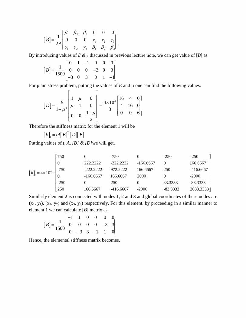
By introducing values of β & γ discussed in previous lecture note, we can get value of [B] as

[ ]0 1 1 0 0 0

1 0 0 0 3 0 31500

3 0 3 0 1 1B

− = − − −

For plain stress problem, putting the values of E and µ one can find the following values.

[ ]4

2

1 0 16 4 04 101 0 4 16 0

1 31 0 0 60 0

2

EDµ

µµ

µ

× = = − −

Therefore the stiffness matrix for the element 1 will be

[ ] [ ] [ ][ ]1

Tk tA B D B=

Putting values of t, A, [B] & [D]we will get,

[ ] 41

750 0 -750 0 -250 -2500 222.2222 -222.2222 -166.6667 0 166.6667-750 -222.2222 972.2222 166.6667 250 -416.6667

4 100 -16

k = × ×6.6667 166.6667 2000 0 -2000

-250 0 250 0 83.3333 -83.3333250 166.6667 -416.6667 -2000 -83.3333 2083.3333

Similarly element 2 is connected with nodes 1, 2 and 3 and global coordinates of these nodes are (x1, y1), (x2, y2) and (x3, y3) respectively. For this element, by proceeding in a similar manner to element 1 we can calculate [B] matrix as,

[ ]1 1 0 0 0 0

1 0 0 0 0 3 31500

0 3 3 1 1 0B

− = − − −

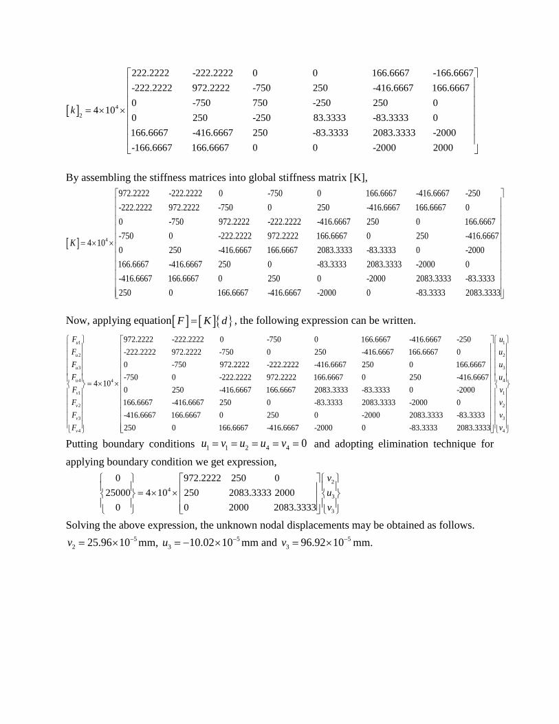
Hence, the elemental stiffness matrix becomes,

[ ] 42

222.2222 -222.2222 0 0 166.6667 -166.6667-222.2222 972.2222 -750 250 -416.6667 166.66670 -750 750 -250 250 0

4 100 250 -250

k = × × 83.3333 -83.3333 0

166.6667 -416.6667 250 -83.3333 2083.3333 -2000-166.6667 166.6667 0 0 -2000 2000

By assembling the stiffness matrices into global stiffness matrix [K],

[ ] 4

972.2222 -222.2222 0 -750 0 166.6667 -416.6667 -250-222.2222 972.2222 -750 0 250 -416.6667 166.6667 00 -750 9

4 10K = × ×

72.2222 -222.2222 -416.6667 250 0 166.6667-750 0 -222.2222 972.2222 166.6667 0 250 -416.66670 250 -416.6667 166.6667 2083.3333 -83.3333 0 -2000166.6667 -416.6667 250 0 -83.3333 2083.3333 -2000 0-416.6667 166.6667 0 250 0 -2000 2083.3333 -83.3333250 0 166.6667 -416.6667 -2000 0 -83.3333 2083.3333

Now, applying equation [ ] [ ] F K d= , the following expression can be written.

1

2

3

4 4

1

2

3

4

972.2222 -222.2222 0 -750 0 166.6667 -416.6667 -250-222.2222 972.2222 -750 0 250 -416.

4 10

u

u

u

u

v

v

v

v

FFFFFFFF

= × ×

6667 166.6667 00 -750 972.2222 -222.2222 -416.6667 250 0 166.6667-750 0 -222.2222 972.2222 166.6667 0 250 -416.66670 250 -416.6667 166.6667 2083.3333 -83.3333 0 -2000166.6667 -416.6667 250 0 -83.3333 2083.3333 -2000 0-416.6667 166.6667 0 250 0 -2000 2083.3333 -83.3333250

1

2

3

4

1

2

3

4 0 166.6667 -416.6667 -2000 0 -83.3333 2083.3333

uuuuvvvv

Putting boundary conditions 1 1 2 4 4 0u v u u v= = = = = and adopting elimination technique for applying boundary condition we get expression,

24

3

3

0 972.2222 250 025000 4 10 250 2083.3333 2000

0 0 2000 2083.3333

vuv

= × ×

Solving the above expression, the unknown nodal displacements may be obtained as follows. 5

2 25.96 10v −= × mm, 53 10.02 10u −= − × mm and 5

3 96.92 10v −= × mm.

Lecture 3: Rectangular Elements The rectangular elements are widely used for solving two dimensional continuums. The main advantage of this type of element is the easy formulation and easy development of computer code. The element stiffness of such elements is derived here using the concept of isoparametric formulation. 5.3.1 Computation of Element Stiffness In case of a four node rectangular element, the geometry and displacement filed can be expressed in terms of their nodal values with the help of interpolation function. As the formulation will be isoparametric, the interpolation function will become same for expressing both the variables. Thus, coordinates and displacements at any point inside the element (Fig. 5.3.1) can be expressed as

1 1 2 2 3 3 4 4

1 1 2 2 3 3 4 4

x N x N x N x N xy N y N y N y N y (5.3.1)

And

1 1 2 2 3 3 4 4

1 1 2 2 3 3 4 4

u N u N u N u N uv N v N v N v N v (5.3.2)

The above equations can be written in matrix form as

1

1

2

1 2 3 4 2

1 2 3 4 3

3

4

4

0 0 0 00 0 0 0

xyx

N N N N yxN N N N xx

yxy

(5.3.3)

And

1

1

2

1 2 3 4 2

1 2 3 4 3

3

4

4

0 0 0 00 0 0 0

uvu

N N N N vuN N N N uv

vuv

(5.3.4)

The shape function four node rectangular element is derived and shown in module 3, lecture 4. However the shape functions are reproduced here for easy reference for the derivation of the stiffness matrix.

1

2

3

4

1 14

1 14

1 14

1 14

i

NN

NNN

x h

x h

x h

x h

(5.3.5)

Fig. 5.3.1 Four node rectangular element

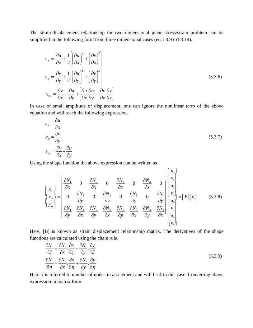
The strain-displacement relationship for two dimensional plane stress/strain problem can be simplified in the following form from three dimensional cases (eq.1.3.9 to1.3.14).

2 2

2 2

12

12

x

y

xy

u u vx x x

v u vy y y

v u u u v vx y x y x y

(5.3.6)

In case of small amplitude of displacement, one can ignore the nonlinear term of the above equation and will reach the following expression.

x

y

xy

uxvyv ux y

ε

ε

γ

∂=∂∂

=∂∂ ∂

= +∂ ∂

(5.3.7)

Using the shape function the above expression can be written as

[ ]

1

131 2 4

2

231 2 4

3

33 31 1 2 2 4 4

4

4

0 0 0 0

0 0 0 0x

y

xy

uvNN N Nux x x xvNN N N B duy y y yvN NN N N N N N

y x y x y x y x uv

εεγ

∂∂ ∂ ∂ ∂ ∂ ∂ ∂ ∂∂ ∂ ∂ = = ∂ ∂ ∂ ∂

∂ ∂∂ ∂ ∂ ∂ ∂ ∂ ∂ ∂ ∂ ∂ ∂ ∂ ∂ ∂

(5.3.8)

Here, [B] is known as strain displacement relationship matrix. The derivatives of the shape functions are calculated using the chain rule.

. .

. .

i i i

i i i

N N Nx yx y

N N Nx yx y

ξ ξ ξ

η η η

∂ ∂ ∂∂ ∂= +

∂ ∂ ∂ ∂ ∂∂ ∂ ∂∂ ∂

= +∂ ∂ ∂ ∂ ∂

(5.3.9)

Here, i is referred to number of nodes in an element and will be 4 in this case. Converting above expression in matrix form

i i i

i ii

N x y N Nx xJ

N NN x yy y

x x x

h hh

(5.3.10)

The matrix [J] is referred to Jacobian matrix which is discussed in Lecture 7, module 3. Using eq. (5.3.1) one can write

31 2 41 2 3 4

NN N Nx x x x x x x x x x

(5.3.11)

Putting the values of the nodal coordinates and shape functions of the four node element in the above equation the following relations will be obtained.

1 1 1 1 1 1 1 10 0

4 4 4 4 2x aa a

h h h hx

(5.3.12a) Similarly,

1 1 1 1 1 1 1 10 0 0

4 4 4 4y b b

h h h hx

(5.3.12b) 1 1 1 1 1 1 1 1

0 0 04 4 4 4

x a a

x x x x

h (5.3.12c)

1 1 1 1 1 1 1 10 0

4 4 4 4 2y bb b

x x x xh

(5.3.12d) Substituting above values in Jacobian matrix the following relations will be obtained.

1

2 002

20 02

aaJ and J

bb

(5.3.13)

Thus, eq.(5.3.10) can be written as

1

22 .0

2 20 .

i i ii

i i i i

N N NNax aJ

N N N Ny b b

x x x

h h h

(5.3.14)

After derivation of the shape functions expressed in eq.(5.3.5), the following values will be obtained.

31 1 2 4

31 1 2 4

1 1 1 12 . ; ; ;2 2 2 2

1 1 1 12 . ; ; ;2 2 2 2

NN N N Nx a a x a x a x a

NN N N Ny b b y b y b y b

h h h hx

x x x xh

(5.3.15)

So, the strain displacement relationship matrix, [B] will become as follows.

[ ]

( ) ( ) ( ) ( )

( ) ( ) ( ) ( )

( ) ( ) ( ) ( ) ( ) ( ) ( ) ( )

1 1 1 10 0 0 0

2 2 2 21 1 1 1

0 0 0 02 2 2 2

1 1 1 1 1 1 1 12 2 2 2 2 2 2 2

a a a a

Bb b b b

b a b a b a b a

η η η η

ξ ξ ξ ξ

ξ η ξ η ξ η ξ η

− − + +− − − + + −

= − − − − + − + + − +− − − −

(5.3.16)

The element stiffness matrix will become

[ ] [ ] [ ][ ] [ ] [ ][ ]T Tk t B D B dx dy t B D B J d dξ η= =∫∫ ∫∫ (5.3.17)

It is seen that the above is expressed in terms of ξ and η and hence can be numerically integrated by the Gauss Quadrature rule. The stiffness matrix for each element can be found which needs to be globally assembled for getting the global stiffness matrix to obtain the solution. The stiffness matrix of higher order rectangular element can be derived in a similar fashion. For example, in case of eight node rectangle element, the size of [B] matrix will become 16 × 3 which was 8 × 3 for four node element. Thus the size of element stiffness for eight node element will become 16 × 16. 5.3.2 Computation of Nodal Loads If a distributed load acts on a side of a four node rectangular element, the nodal load vector can be calculated the similar procedure as discussed in case of triangular element. If an element as shown below is subjected to a linearly varying intensities of load at its one side, then the magnitude of this at any point on the side can be expressed by its interpolation function as follows.

2

3

1 12 2

xx

x

qq

qη η − + =

(5.3.18)

Here, qx2 and qx3 are the force intensities per unit length at nodes 2 and 3 respectively. The load at nodes can be calculated from the following expression.

2 1S

x xF N q d= Γ∫ (5.3.19)

As ξ=1 along the side 2-3, the interpolation function will become

( )( )

( )( )

( )( )

( )( )

( )

( )2

1 104

1 1 14 2

1 1 14 2

01 14

SN

ξ η

ξ η η

ξ η η

ξ η

− − + − − = =

+ + +

− +

(5.3.20)

If the element thickness is t, then dΓ1 =t.dl. Thus the eq.(5.3.19) can be replaced as

( )

( )

12

31

01

1 122 21

20

xx

x

qF t dl

q

ηη η

η

+

−

−

− + = +

∫ (5.3.21)

Fig. 5.3.2 Varying load on a four node element After integrating the above expression, the nodal load vector along x direction will become as follows.

2 3

2 3

02

230

x xx

x x

q qtFq q

+ = +

(5.3.22)

Lecture 4: Numerical Evaluation of Element Stiffness Derivation of element stiffness for a four node rectangle element has been demonstrated in last lecture. The stiffness matrix of each element can be calculated easily by developing a suitable computer algorithm. To help students for developing their own computer code, a numerical example has been solved and demonstrated here. 5.4.1 Numerical Example Calculate the stiffness matrix for the given four node rectangular element by the Gauss Quadrature integration rule using one point and two point formula assuming plane stress formulation. Consider, the thickness of element = 20 cm, E=2 × 103 kN/cm2 and µ =0.

Fig. 5.4.1 Element Dimension

5.4.2 Evaluation of Stiffness using One Point Gauss Quadrature For the calculation of stiffness matrix, first, 1×1 Gauss Quadrature integration procedure has been carried out. Thus, the natural coordinate of the sampling point will become 0,0 and weight will become 2.0 which is shown in the figure below.

Fig. 5.4.2 Natural coordinates for one point Gauss Quadrature

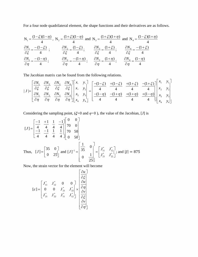
For a four node quadrilateral element, the shape functions and their derivatives are as follows.

4)1)(1(N1

ηξ −−= ,

4)1)(1(N2

ηξ −+= and

4)1)(1(N3

ηξ ++= and

4)1)(1(N4

ηξ +−=

4)1(1 ξ

ξ−−

=∂∂N ;

4)1(2 ξ

ξ−

=∂∂N ;

4)1(3 ξ

ξ+

=∂∂N ;

4)1(4 ξ

ξ+−

=∂∂N

4)1(1 η

η−−

=∂∂N ;

4)1(2 η

η+−

=∂∂N ;

4)1(3 η

η+

=∂∂N ;

4)1(4 η

η−

=∂∂N

The Jacobian matrix can be found from the following relations.

1 1

2

1 131 2 4

2 2 2

3 331 2 4 3 3

4 4 4 4

(1 ) (1 ) (1 ) (1 )4 4 4 4| |

(1 ) (1 ) (1 ) (1 )4 4 4 4

x yx yNN N Nx y x y

Jx yNN N N x yx y x y

ξ ξ ξ ξξ ξ ξ ξ

η η η ηη η η η

∂∂ ∂ ∂ − − + − + + − + ∂ ∂ ∂ ∂ = = ∂ − − − + + + + −∂ ∂ ∂ ∂ ∂ ∂ ∂

Considering the sampling point, (ξ=0 and η=0 ), the value of the Jacobian, [J] is

−−

−+−

=

500507007000

41

41

41

41

41

41

41

41

][J

Thus,

=

250035

][J and * *

1 11 12* *21 22

1 035[ ]

1025

J JJ

J J−

= =

; and |𝐽| = 875

Now, the strain vector for the element will become

∂∂∂∂∂∂∂∂

×

=

η

ξ

η

ξ

ε

v

v

u

u

JJJJJJ

JJ

*12

*11

*22

*21

*22

*21

*12

*11

0000

][

∂∂

∂∂

∂∂

∂∂

∂∂

∂∂

∂∂

∂∂

∂∂

∂∂

∂∂

∂∂

∂∂

∂∂

∂∂

∂∂

×

=

4

4

3

3

2

2

1

1

4321

4321

4321

4321

*12

*11

*22

*21

*22

*21

*12

*11

0000

0000

0000

0000

0000

][

vuvuvuvu

NNNN

NNNN

NNNN

NNNN

JJJJJJ

JJ

ηηηη

ξξξξ

ηηηη

ξξξξ

ε

[ ] ]['0000

][*12

*11

*22

*21

*22

*21

*12

*11

dBdBJJJJJJ

JJ=×

=ε

−−

−−

−−

−−

=

410

410

410

410

410

410

410

410

0410

410

410

41

0410

410

410

41

][ /B

and [ ]'

0351

2510

251000

000351

][ BB

=

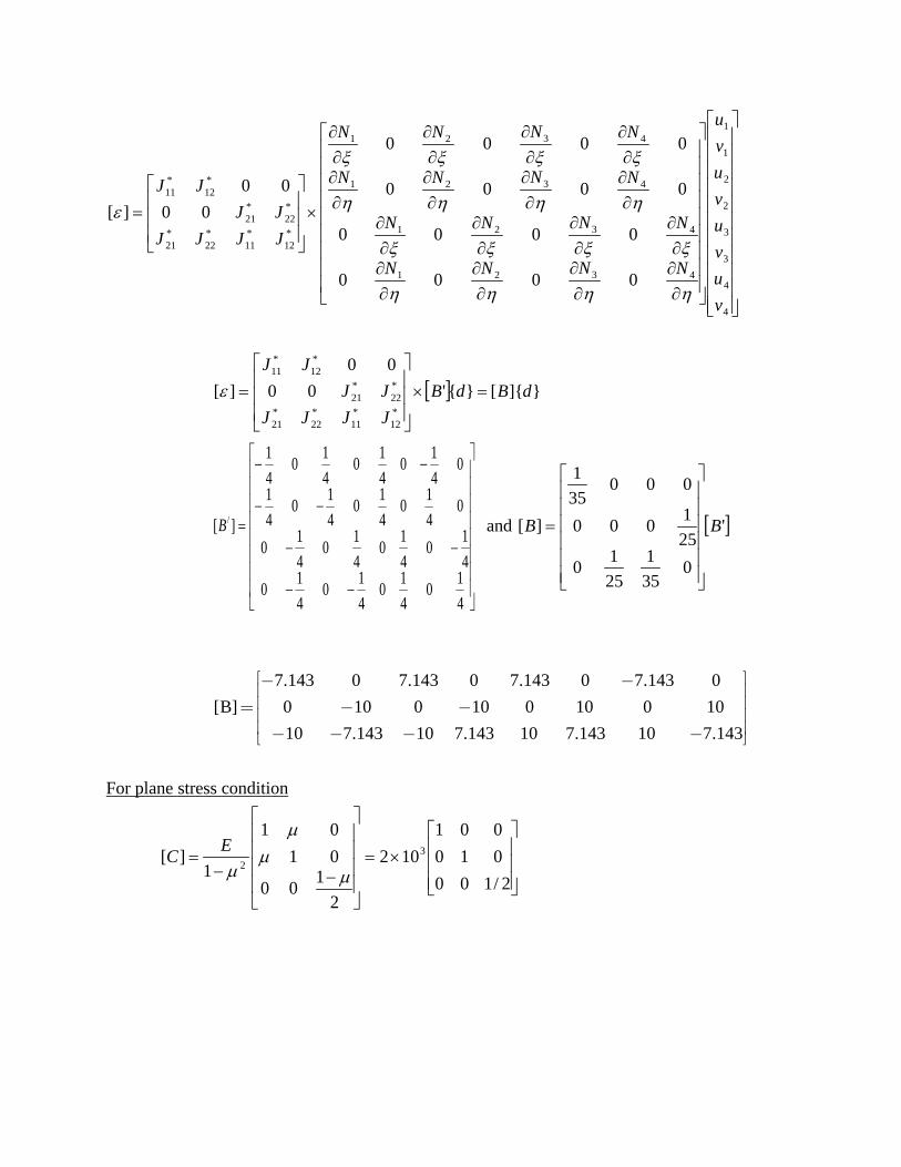
7.143 0 7.143 0 7.143 0 7.143 0[B] 0 10 0 10 0 10 0 10

10 7.143 10 7.143 10 7.143 10 7.143

For plane stress condition

×=

−−=

2/100010001

102

2100

0101

1][ 3

2µ

µµ

µEC

×

×=

2/100010001

102]][[ 3BC

7.143 0 7.143 0 7.143 0 7.143 00 10 0 10 0 10 0 1010 7.143 10 7.143 10 7.143 10 7.143

Assume the values of gauss weight, w = 2, the stiffness matrix [k] at this sampling point is [ ] [ ] [ ] [ ] | |Tk tw B C B J= , Where t is thickness of the element. Thus,

[ ] 3

7.143 0 100 10 7.143

7.143 0 101 0 0

0 10 7.14320 2 875 2 10 10 0 1 0

7.143 0 100 0 1/ 2

0 10 7.1437.143 0 4

0 10 7.143

7.143 0 7.143 0 7.143 0 7.143 00 10 0 10 0 10 0 1010 7.143 10 7.143 10 7.

k

− − − − −

− = × × × × × ×

−

− − −

× − −− − − 143 10 7.143

−

3

7.071 2.5 0.714 2.5 7.071 2.5 0.714 2.52.5 8.785 2.5 5.214 2.5 8.785 2.5 5.2140.714 2.5 7.071 2.5 0.714 2.5 7.071 2.5

2.5 5.214 2.5 8.785 2.5 5.214 2.5 8.78510

7.071 2.5 0.714 2.5 7.071 2.5 0.714 2.52.5 8.785 2.5 5

− − − −− − −

− − − −− − − −

= ×− − − −− − − − .214 2.5 8.785 2.5 5.2140.714 2.5 7.071 2.5 0.714 2.5 7.071 2.5

2.5 5.214 2.5 8.785 2.5 5.214 2.5 8.785

− − − −

− − − −

5.4.3 Evaluation of Stiffness using Two Point Gauss Quadrature

In this case, 2×2 Gauss Quadrature integration procedure has been carried out to the calculate the stiffness matrix of the same element for a comparison. The natural coordinate of the sampling point is shown in the figure below.

Fig. 5.4.3 Natural Coordinates for Two Points Gauss Quadrature

The natural co-ordinates of the sampling points for 2×2 Gauss Quadrature integration are

1 +0.57735 +0.57735 2 -0.57735 +0.57735 3 -0.57735 -0.57735 4 +0.57735 -0.57735

For a four node quadrilateral element, the shape functions and their derivatives are as follows.

4)1)(1(N1

ηξ −−= ,

4)1)(1(N2

ηξ −+= ,

4)1)(1(N3

ηξ ++= and

4)1)(1(N4

ηξ +−=

4)1(1 ξ

ξ−−

=∂∂N ;

4)1(2 ξ

ξ−

=∂∂N ;

4)1(3 ξ

ξ+

=∂∂N ;

4)1(4 ξ

ξ+−

=∂∂N

4)1(1 η

η−−

=∂∂N ;

4)1(2 η

η+−

=∂∂N ;

4)1(3 η

η+

=∂∂N ;

4)1(4 η

η−

=∂∂N

The Jacobian matrix will be

1 1

2

1 131 2 4

2 2 2

3 331 2 4 3 3

4 4 4 4

(1 ) (1 ) (1 ) (1 )4 4 4 4| |

(1 ) (1 ) (1 ) (1 )4 4 4 4

x yx yNN N Nx y x y

Jx yNN N N x yx y x y

ξ ξ ξ ξξ ξ ξ ξ

η η η ηη η η η

∂∂ ∂ ∂ − − + − + + − + ∂ ∂ ∂ ∂ = = ∂ − − − + + + + −∂ ∂ ∂ ∂ ∂ ∂ ∂

(a) At sampling point 1, (ξ=0.57735, η=0.57735) The value of the Jacobian, [J] at sampling point 1 will become

−++++−−−

+−++−+−−

=

500507007000

4)0.577351(

4)0.577351(

4)0.577351(

4)0.577351(

4)0.577351(

4)0.577351(

4)0.577351(

4)0.577351(

][J

Thus,

=

250035

][J and * *

1 11 12* *21 22

1 035[ ]

1025

J JJ

J J−

= =

; Thus |𝐽| = 875

∂∂∂∂∂∂∂∂

×

=

η

ξ

η

ξ

ε

v

v

u

u

JJJJJJ

JJ

*12

*11

*22

*21

*22

*21

*12

*11

0000

][

∂∂

∂∂

∂∂

∂∂

∂∂

∂∂

∂∂

∂∂

∂∂

∂∂

∂∂

∂∂

∂∂

∂∂

∂∂

∂∂

×

=

4

4

3

3

2

2

1

1

4321

4321

4321

4321

*12

*11

*22

*21

*22

*21

*12

*11

0000

0000

0000

0000

0000

][

vuvuvuvu

NNNN

NNNN

NNNN

NNNN

JJJJJJ

JJ

ηηηη

ξξξξ

ηηηη

ξξξξ

ε

[ ] ]['0000

][*12

*11

*22

*21

*22

*21

*12

*11

dBdBJJJJJJ

JJ=×

=ε

1 0.57735 1 0.57735 1 0.57735 1 0.577350 0 0 04 4 4 4

1 0.57735 1 0.57735 1 0.57735 1 0.577350 0 0 04 4 4 4[ ]

1 0.57735 1 0.57735 1 0.57735 1 0.577350 0 0 04 4 4 4

1 0.57735 1 0.57735 1 0.57735 1 0.577350 0 0 04 4 4 4

B

− − + +− −

− + + −− −′ = − − + + − −

− + + −

− −

0.1057 0 0.1057 0 0.3943 0 0.3943 00.1057 0 0.3943 0 0.3943 0 0.1057 0

[ ']0 0.1057 0 0.1057 0 0.3943 0 0.39430 0.1057 0 0.3943 0 0.3943 0 0.1057

B

− − − − = − − − −

Thus,

1 0 0 0 0.1057 0 0.1057 0 0.3943 0 0.3943 0350.1057 0 0.3943 0 0.3943 0 0.1057 01[ ] 0 0 0

0 0.1057 0 0.1057 0 0.3943 0 0.3943251 1 0 0.1057 0 0.3943 0 0.3943 0 0.10570 025 35

B

− − − − = × − − − −

−−−−−−

−−=

0113.00042.00113.00158.0003.00158.0003.00042.00042.000158.000158.000042.0000113.000113.00003.00003.0

][B

For plane stress condition

×=

−−=

2/100010001

102

2100

0101

1][ 3

2µ

µµ

µEC

×

×=

2/100010001

102]B][C[ 3

−−−−−−

−−

0113.00042.00113.00158.0003.00158.0003.00042.00042.000158.000158.000042.0000113.000113.00003.00003.0

The values of gauss weights are wi=wj=1.0. Therefore, the stiffness matrix [k] at this sampling

point is [ ] [ ] [ ] [ ] | |Ti j ij ij ijk tw w B C B J= , where t is thickness of the element. Thus at sampling point

1,

[ ] 31

0.003 0 0.00420 0.0042 0.003

0.003 0 0.01581 0 0

0 0.0158 0.00320 1 1 875 2 10 0 1 0

0.0113 0 0.01580 0 1/ 2

0 0.0158 0.01130.0113 0 0.0042

0 0.0042 0.0113

0.003 0 0.003 0 0.0113 0 0.

k

− − − − −

− = × × × × × × × ×

−

− − − 0113 0

0 0.0042 0 0.0158 0 0.0158 0 0.00420.0042 0.003 0.0158 0.003 0.0158 0.0113 0.0042 0.0113

− − − − − −

[ ] 41

0.0632 0.0223 0.0848 0.0223 0.2358 0.0834 0.0878 0.08340.0785 0.0834 0.2174 0.0834 0.2929 0.0223 0.0030

0.4672 0.0834 0.3162 0.3109 0.2358 0.31090.8866 0.0834 0.8111 0.0223 0.2929

100.8795 0.3109 0.3275 0.31

k

− − −− − − −

− − − −− −

= ×− − 09

1.0927 0.0834 0.01130.4755 0.0834

0.2847

sym

−

(b) At sampling point 2, (ξ=-0.57735, η=0.57735) The value of the Jacobian, [J] at sampling point 2 can be calculated in a similar way and finally the strain-displacement relationship matrix and then the stiffness matrix [k2] can be evaluated and is shown below.

[ ] 32

0.0113 0 0.00420 0.0042 0.0113

0.0113 0 0.01580 0.0158 0.0113

20 1 1 875 2 100.003 0 0.0158

0 0.0158 0.0030.003 0 0.0042

0 0.0042 0.0030

0.0113 0 0.0113 0 0.0030 0 0.0030 00 0.0042 0 0.015

k

− − − − − − = × × × × × × −

− − −

− − 8 0 0.0158 0 0.00420.0021 0.0056 0.0079 0.0056 0.0079 0.0015 0.0021 0.0015

− − − −

[ ] 42

0.4756 0.0833 0.3276 0.0833 0.2357 0.0223 0.0878 0.02230.2847 0.3110 0.0112 0.3110 0.2929 0.0833 0.0030

0.8797 0.3110 0.3164 0.0833 0.2357 0.08331.0930 0.3110 0.8113 0.0833 0.2929

100.4673 0.0833 0.0848 0.08

k

− − − −− − − −

− − − −− −

= ×− 33

0.8868 0.0223 0.21740.0632 0.0223

0.0785

sym

−

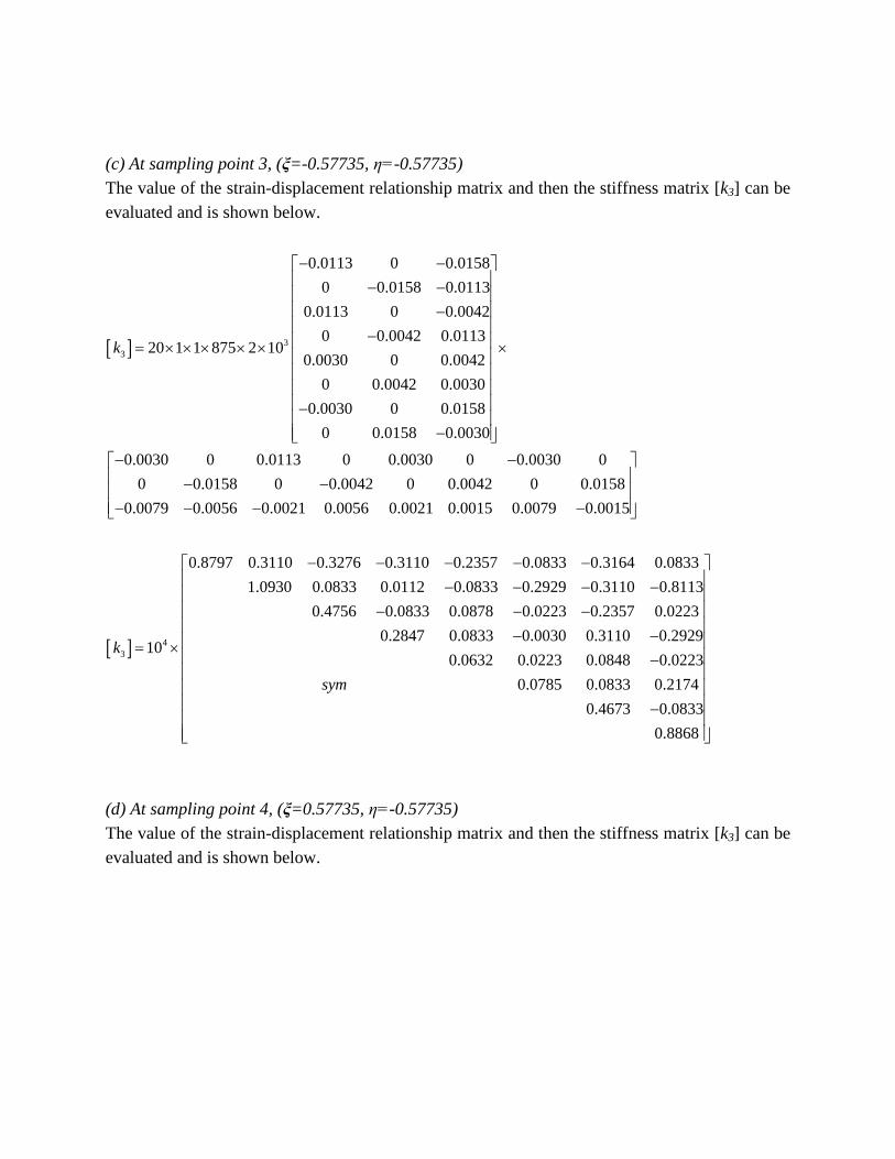
(c) At sampling point 3, (ξ=-0.57735, η=-0.57735) The value of the strain-displacement relationship matrix and then the stiffness matrix [k3] can be evaluated and is shown below.

[ ] 33

0.0113 0 0.01580 0.0158 0.0113

0.0113 0 0.00420 0.0042 0.0113

20 1 1 875 2 100.0030 0 0.0042

0 0.0042 0.00300.0030 0 0.0158

0 0.0158 0.0030

0.0030 0 0.0113 0 0.0030 0 0.0030 00 0.0158 0 0.

k

− − − − − − = × × × × × × −

− − −

− − 0042 0 0.0042 0 0.01580.0079 0.0056 0.0021 0.0056 0.0021 0.0015 0.0079 0.0015

− − − −

[ ] 43

0.8797 0.3110 0.3276 0.3110 0.2357 0.0833 0.3164 0.08331.0930 0.0833 0.0112 0.0833 0.2929 0.3110 0.8113

0.4756 0.0833 0.0878 0.0223 0.2357 0.02230.2847 0.0833 0.0030 0.3110 0.2929

100.0632 0.0223 0.0848 0.02

k

− − − − −− − − −

− − −− −

= ×− 23

0.0785 0.0833 0.21740.4673 0.0833

0.8868

sym

−

(d) At sampling point 4, (ξ=0.57735, η=-0.57735) The value of the strain-displacement relationship matrix and then the stiffness matrix [k3] can be evaluated and is shown below.

[ ] 34

0.0030 0 0.01580 0.0158 0.0030

0.0030 0 0.00420 0.0042 0.0030

20 1 1 875 2 100.0113 0 0.0042

0 0.0042 0.01130.0113 0 0.0158

0 0.0158 0.0113

0.0030 0 0.0030 0 0.0113 0 0.0113 00 0.0158 0 0.

k

− − − − − − = × × × × × × −

− − −

− − 0042 0 0.0042 0 0.01580.0079 0.0015 0.0021 0.0015 0.0021 0.0056 0.0079 0.0056

− − − −

[ ] 44

0.4673 0.0833 0.0848 0.0833 0.2357 0.3110 0.3164 0.31100.8868 0.0223 0.2174 0.0223 0.2929 0.0833 0.8113

0.0632 0.0223 0.0878 0.0833 0.2357 0.08330.0785 0.0223 0.0030 0.0833 0.2929

100.4756 0.0833 0.3276 0.08

k

− − − −− − − −

− − −− −

= ×− − 33

0.2847 0.3110 0.01120.8797 0.3110

1.0930

sym

−

The stiffness matrix of the element can be computed as the sum of the values at the four sampling points: 1 2 3 4[ ] [ ] [ ] [ ] [ ]k k k k k= + + + . Thus, the final value of the stiffness matrix will become

[ ] 4

1.8857 0.5000 0.4857 0.5000 0.9429 0.5000 0.4571 0.31102.3429 0.5000 0.4571 0.5000 1.1714 0.5000 1.6286

1.8857 0.5000 0.4571 0.5000 0.9429 0.50002.3429 0.5000 1.6286 0.5000 1.1714

101.8857 0.5000 0.4857 0.

k

− − − − −− − − −

− − − −− − −

= ×− − 5000

2.3429 0.5000 0.45711.8857 0.5000

2.3429

sym

−

Lecture 5: Computation of Stresses, Geometric Nonlinearity and Static Condensation 5.5.1 Computation of Stresses After solving the static equation of F = [K]d, the nodal displacement d can be obtained in global coordinate system. The element nodal displacement d can then be calculated from the

nodal connectivity of the element. Using strain-displacement relation and then stress-strain relation, the stress at the element level are derived.

σ= DεD B d (5.5.1)

Here, is the stress at the Gauss point of the element as the sampling points for the integration

has been considered as Gauss points. Here, [D] is the constitutive matrix, [B] is the strain displacement matrix of the element. As a result these stresses at Gauss points need to extrapolate to the corresponding nodes of the element. It is well established that 2 × 2 Gauss integration points are the optimal sampling points for two dimensional isoparametric elements. The ‘local stress smoothing’ is a technique that can be used to extrapolate stresses computed at Gauss points to nodal points. The stresses are computed at four Gauss points (I, II, III and IV) of an 8

node element as shown in Fig. 5.5.1. For example, at point III, r = s =1 an d ξ = η = 31 .

Therefore the factor of proportionality is 3 ; i.e.,

3ξ=r and 3η=s (5.5.2) Stresses at any point P in the element are found by the usual shape function as

∑ ′= idiP N σσ for i = 1,2,3,4 (3.5.3)

In the above equation, Pσ is yx σσ , and xyτ at point P. diN ′ are the bilinear shape functions

written in terms of r and s rather than ξ and η as

( )( )srNdi ±±=′ 1141 (5.5.4)

diN ′ are evaluated at r and s coordinates of point P. Let the point P coincides with the corner 1.

To calculate stress 1xσ at corner 1 from xσ values at the four Gauss points, substitution of r and s into the shape functions will give

xIVxIIIxIIxIxI σσσσσ 500.0134.0500.08666.1 −+−= (5.5.5)

Fig. 5.5.1 Natural coordinate systems used in extrapolation of stresses from Gauss points The resultant extrapolation matrix thus obtained may be written as

( ) ( )( ) ( )

( ) ( )( ) ( )

( ) ( ) ( ) ( )( ) ( ) ( ) ( )( ) ( ) ( ) ( )( ) ( ) ( ) ( )

+−−+++−−−++−−−+++−−−−+−−−−+−−−−+

=

IV

III

II

I

σσσσ

σσσσσσσσ

4314314314314314314314314314314314314314314314312315.02315.0

5.02315.02312315.02315.0

5.02315.0231

8

7

6

5

4

3

2

1

(5.5.6)

Here, 1σ , 2σ …….. 8σ are the smoothened nodal values and Iσ … IVσ are the stresses at the Gauss points. Smoothened nodal stress values for four node rectangular element can be also be evaluated in a similar fashion. The relation between the stresses at Gauss points and nodal point for four nodel element will be

1 I

2 II

3 III

IV4

3 1 3 11 12 2 2 2

1 3 1 31 12 2 2 2

3 1 3 11 12 2 2 2

1 3 1 31 12 2 2 2

(5.5.7)

The stress at particular node joining with more than one element will have different magnitude as calculated from adjacent elements (Fig. 5.5.2(a)). The stress resultants are then modified by finding the average of resultants of all elements meeting at a common node. A typical stress distribution for adjacent elements is shown in Fig. 5.5.2(b) after stress smoothening.

Fig. 5.5.2 Stress smoothening at common node 5.5.2 Geometric Nonlinearity As discussed earlier, nonlinear analysis is mainly of two types: (i) Geometric nonlinearity and (ii) Material nonlinearity. For geometric nonlinearity consideration, the relation between strain and displacement is of utmost importance in the finite element formulation for stress analysis problems. In case of plane stress/strain problem, the nonlinear term of the strain expression are dropped for the sake of simplicity in the analysis. However, for large displacement problems, the nonlinear strain term plays a vital role to obtain accurate response. The generalized strain-displacement relations for the two-dimensional plane stress/strain problems are rewritten here to derive the nonlinear solution.

2 2

2 2

12

12

x

y

xy

u u vx x x

v u vy y y

v u u u v vx y x y x y

ε

ε

γ

∂ ∂ ∂ = + + ∂ ∂ ∂ ∂ ∂ ∂

= + + ∂ ∂ ∂ ∂ ∂ ∂ ∂ ∂ ∂

= + + + ∂ ∂ ∂ ∂ ∂ ∂

(5.5.8)

The displacements at any point inside the node are expressed in terms of their nodla displacements. Thus,

[ ] 1

n

i i i ii

u N u N u=

= =∑ and [ ] 1

n

i i i ii

v N v N v=

= =∑ (5.5.9)

Therefore,

[ ] [ ]

[ ]

[ ]

[ ]

1

1

2

2

ii i

i

i

i

Nu u B ux xv B vxu B uyv B vy

∂∂= =

∂ ∂∂

=∂∂

=∂∂

=∂

(5.5.10)

Here, [B1] and [B2] are the derivative of the shape function [Ni] with respect to x and y respectively. The vectors ui and vi represent the nodal displacements vectors in x and y directions respectively. The vector of strains at any point inside an element, ε may be expressed in terms of nodal displacement as

[ ] B dε =

(5.5.11) where [B] is the strain displacement matrix. d is the nodal displacement vector and may be expressed as

i

i

ud

v =

(5.5.12) The matrix [B] may be expressed with two components as

[ ] [ ] [ ]l nlB B B= +

(5.5.13) where, [Bl] and [Bnl] are the linear and nonlinear part of the strain-displacement matrix respectively and are expressed as follows:

[ ][ ] [ ][ ] [ ][ ] [ ]

=

12

2

1

00

BBB

BBl

(5.5.14) and

[ ]

[ ] [ ] [ ] [ ]

[ ] [ ] [ ] [ ] [ ] [ ] [ ] [ ]

=

1212

2222

1111

21

21

21

21

BBvBBu

BBvBBu

BBvBBu

BTTTT

TTTT

TTTT

nl

(5.5.15) 5.5.2.1 Steps to include effect of geometrical nonlinearity The nonlinear geometric effect of the structure at a particular instant of time can be obtained by performing the following steps.

1. Calculation of displacement d1 considering linear part of strain matrix [Bl]. 2. Evaluation of nonlinear part of the strain matrix [Bnl] (eq5.5.15) adopting d1 from

previous step. 3. Evaluation of total strain matrix [B] = [Bl] + [Bnl]. 4. Calculation of displacement d2 considering both linear and nonlinear part of strain

matrix [B]. 5. Repetition of steps 2 to 4 with d2, from which modified displacement, d3 are

obtained. 6. Step 5 is carried out until the displacements for two consecutive iteration converge

i.e.,

1j j

j

d d

dε−

−<

Where ε is any pre-assigned small value and j is the number of iterations. 5.5.3 Static Condensation The higher order Lagrangian elements (i.e., nine node, sixteen node rectangular element) contain number of internal nodes. This is necessary sometimes for the completeness of the desired polynomial used in displacement function for derivation of interpolation function. These internal nodes are not connected to the adjoining elements in the assemblage (Fig. 5.5.3).

Fig. 5.5.3 Internal nodes of Nine node elements Thus, the displacements of these nodes are not required to formulate overall equilibrium equations of the structure. This limits the usefulness of these elements. A technique known as “static condensation” can be used to suppress the degrees of freedom associated with the internal nodes in the final computation. The technique of static condensation is explained below. The equilibrium equation for a system are expressed in the finite element form as

F = K d (5.5.16)

Where, F, [K] and d are the load vector, stiffness matrix and displacement vector for the entire structure. The above equation can be rearranged by separating the relevant terms corresponding to internal and external nodes of the elements.

i ii ie i

e ei ee e

F K K d=

F K K d

(5.5.17)

Here, di and de are the displacement vectors corresponding to internal and external nodes respectively. Similarly, Fi and Fe are force vectors corresponding to internal and external nodes. Now, the above expression can be written in the following form separately.

i ii i ie eF K d K d (5.5.18)

e ei i ee eF K d K d (5.5.19)

The stiffness matrix and nodal load vector corresponds to the internal nodes can be separated out. For this, eq.(5.5.18) can be rewritten as

1 1i ii i ii ie ed K F K K d (5.5.20)

Substituting the value of di obtained from the above equation in eq.(5.5.19), the following expression will be obtained.

1 1e ei ii i ii ie e ee eF K K F K K d K d (5.5.21)

Here, the equations are reduced to a form involving only the external nodes of the elements. The above reduced substructure equations are assembled to achieve the overall equations involving only the boundary unknowns. Thus the above equation can be rewritten as

1 1e ei ii i ee ei ii ie e eF K K F K K K K d d (5.5.22)

Or

c c eF = K d (5.5.23)

Where, and-1 -1c e ei ii i c ee ei ii ie eF = F - K K F K = K - K K K d . Here, [Kc]

is called condensed or reduced stiffness matrix and Fc is the condensed or effective nodal load vector corresponding to external nodes of the elements. In this process, the size of the matrix for inversion will be comparatively small. The unknown displacements of the exterior nodes, de can be obtained by inverting the matrix [Kc] in eq.(5.5.23). Once, the values of de are obtained, the displacements of internal nodes di can be found from eq.(5.5.20).

Lecture 6: Axisymmetric Element 5.6.1 Introduction Many three-dimensional problems show symmetry about an axis of rotation. If the problem geometry is symmetric about an axis and the loading and boundary conditions are symmetric about the same axis, the problem is said to be axisymmetric. Such three-dimensional problems can be solved using two-dimensional finite elements. The axisymmetric problem are most conveniently defined by polar coordinate system with coordinates (r, θ, z) as shown in Fig. 5.6.1. Thus, for axisymmetric analysis, following conditions are to be satisfied.

1. The domain should have an axis of symmetry and is considered as z axis. 2. The loadings on the domain has to be symmetric about the axis of revolution, thus they

are independent of circumferential coordinate θ. 3. The boundary condition and material properties are symmetric about the same axis and

will be independent of circumferential coordinate.

Fig. 5.6.1 Cylindrical coordinates

Axisymmetric solids are of total symmetry about the axis of revolution (i.e., z-axis), the field variables, such as the stress and deformation is independent of rotational angle θ. Therefore, the field variables can be defined as a function of (r, z) and hence the problem becomes a two dimensional problem similar to those of plane stress/strain problems. Axisymmetric problems includes, circular cylinder loaded with uniform external or internal pressure, circular water tank, pressure vessels, chimney, boiler, circular footing resting on soil mass, etc. 5.6.2 Relation between Strain and Displacement An axisymmetric problem is readily described in cylindrical polar coordinate system: r, z and θ. Here, θ measures the angle between the plane containing the point and the axis of the coordinate

P( r,z, )θ•

system. At θ = 0, the radial and axial coordinates coincide with the global Cartesian X and Y coordinates. Fig. 5.6.2 shows a cylindrical coordinate system and the definition of the position vectors. Let ˆˆ ˆr, z and be unit vectors in the radial, axial, and circumferential directions at a point in the cylindrical coordinate system.

Fig. 5.6.2 Cylindrical Coordinate System If the loading consists of radial and axial components that are independent of θ and the material is either isotropic or orthotropic and the material properties are independent of θ, the displacement at any point will only have radial (𝑢𝑟) and axial (𝑢𝑧) components. The only stress components that will be nonzero are 𝜎𝑟𝑟 , 𝜎𝑧𝑧, 𝜎𝜃𝜃 𝑎𝑛𝑑 𝜏𝑟𝑧 .

(a) Element in r-z plane (b) Element in r-θ plane

Fig. 5.6.3 Deformation of the axisymmetric element

A differential element of the body in the r-z plane is shown in Fig. 5.6.3(a). The element undergoes deformation in the radial direction. Therefore, it initiates increase in circumference and associated circumferential strain. Let denote the radial displacement as u, the circumferential displacement as v, and the axial displacement as w. Dashed line represents the deformed positions of the body in Fig. 5.6.3(b). The radial strain can be calculated from the above diagram as

r1 u uε = u+×dr - u =dr r r

(5.6.1)

Since the rz plane is effectively the same as a rectangular coordinate system, the axial strain will become

z1 w wε = w+×dz - w =dz z z

(5.6.2)

Considering the original arc length versus the deformed arc length, the differential element undergoes an expansion in the circumferential direction. Before deformation, let the arc length is assumed as ds = rdθ. After deformation, the arc length will become ds = (r+u) dθ. Thus, the tangential strain will be

r +u d - rd uε =rd r

(5.6.3)

Similarly, the shear strain will be

rz

r z0 and 0

u wz r

(5.6.4)

Thus, there are four strain components present in this case and is given by

0

0

1 0

r

z

rz

ur rw

uz zwu

r ru wz r z r

θ

εε

εεγ

∂ ∂ ∂ ∂ ∂ ∂ ∂ ∂= = =

∂ ∂ ∂ ∂ +

∂ ∂ ∂ ∂

(5.6.5)

5.6.3 Relation between Stress and Strain The stress strain relation for axisymmetric case can be derived from the three dimensional constitutive relations. We know the stress-strain relation for a three-dimensional solid is

⎩⎪⎨

⎪⎧𝜎𝑥𝜎𝑦𝜎𝑧𝜏𝑥𝑦𝜏𝑦𝑧𝜏𝑧𝑥⎭

⎪⎬

⎪⎫

= 𝐸(1+𝜇)(1−2𝜇)

⎣⎢⎢⎢⎢⎢⎢⎢⎢⎡1 − 𝜇 𝜇 𝜇 0 0 0

𝜇 1 − 𝜇 𝜇 0 0 0

𝜇 𝜇 1 − 𝜇 0 0 0

0 0 0 1−2𝜇2

0 0

0 0 0 0 1−2𝜇2

0

0 0 0 0 0 1−2𝜇2 ⎦⎥⎥⎥⎥⎥⎥⎥⎥⎤

⎩⎪⎨

⎪⎧

ϵ𝑥ϵ𝑦ϵ𝑧𝜈𝑥𝑦𝜈𝑦𝑧𝜈𝑧𝑥⎭

⎪⎬

⎪⎫

(5.6.6) The stresses acting on a differential volume of an axisymmetric solid under axisymmetric loading is shown in Fig. 5.6.4.

Fig. 5.6.4 Stresses acting on a differential volume

Now, comparing the stress-strain components present in the axisymmetric case, the stress-strain relation can be expressed from the above expression as follows

⎩⎪⎨

⎪⎧𝜎𝑟

𝜎𝑧

𝜎𝜃

𝜏𝑟𝑧⎭⎪⎬

⎪⎫

= 𝐸(1+𝜇)(1−2𝜇)

⎣⎢⎢⎢⎢⎡1 − 𝜇 𝜇 𝜇 0

𝜇 1 − 𝜇 𝜇 0

𝜇 𝜇 1 − 𝜇 0

0 0 0 1−2𝜇2 ⎦⎥⎥⎥⎥⎤

⎩⎪⎨

⎪⎧𝜀𝑟

𝜀𝑧

𝜀𝜃

𝜈𝑟𝑧⎭⎪⎬

⎪⎫

(5.6.7)

Thus, the constitutive matrix [D] for the axisymmetric elastic solid will be

[D] = 𝐸(1+𝜇)(1−2𝜇)

⎣⎢⎢⎢⎢⎡1 − 𝜇 𝜇 𝜇 0

𝜇 1 − 𝜇 𝜇 0

𝜇 𝜇 1 − 𝜇 0

0 0 0 1−2𝜇2 ⎦⎥⎥⎥⎥⎤

(5.6.8)

5.6.4 Axisymmetric Shell Element A cylindrical liquid storage container like structures (Fig. 5.6.5) may be idealized using axisymmetric shell element for the finite element analysis. It may be noted that the liquid in the container may be idealized with two dimensional axisymmetric elements. Let us consider the radius, height and, thickness of the circular tank are R, H and h respectively.

Fig. 5.6.5 Thin wall cylindrical container

The strain energy of the axisymmetric shell element (Fig. 5.6.6) including the effect of both stretching and bending are expressed as

( )0

H

y yθ θ y y1U = Nε + N ε + M χ 2πRdy2 ∫ (5.6.9)

Here, Ny and Nθ are the membrane force resultants and My is the bending moment resultant. The shell is assumed to be linearly elastic, homogeneous and isotropic. Thus the force and moment resultants can be expressed in terms of the mid-surface change in curvature χy as follows.

Fig 5.6.6 Axisymmetric plate element Here, the strain-displacement relation is given by

[ ] σ ε D= (5.6.10)

In which,

y

yM

NNθσ

=

, y

y

θ

εε ε

χ

=

and [ ] 22

1 01 0

10 0

12

EhDh

µ

µµ

= −

(5.6.11)

The generalized strain vector can be expressed in terms of the displacement vectors as follows.

[ ] B dε = (5.6.12)

Where,

dv

u

=

and [ ]2

2

0

1 0

0

y

R

y

B

∂ ∂ =

∂ − ∂

(5.6.13)

Here, u and v are the displacement components in two perpendicular directions. With the use of stress and strain vectors, the potential energy expression are written in terms of displacement vectors as

[ ] [ ][ ] ( )0

TH

Td B D B d1U = 2πR dy2× ∫ (5.6.14)

Thus, the element stiffness are derived as

[ ] [ ] [ ][ ]0

2π H

Tk R B D B dy= ∫ (5.6.15)

Similarly, neglecting the rotary inertia, the kinetic energy can be expressed as

[ ] [ ] ( )0

THTd N m N1T = 2πR dyd

2× ∫ (5.6.16)

Where, m denotes the mass of the shell element per unit area and d represents the velocity

vector. Thus, the element mass matrix is given by

[ ] [ ] [ ]0

2π eL

TM Rm N N dy = ∫ (5.6.17)

Lecture 7: Finite Element Formulation of Axisymmetric Element Finite element formulation for the axisymmetric problem will be similar to that of the two dimensional solid elements. As the field variables, such as the stress and strain is independent of rotational angle θ, circumferential displacement will not appear. Thus, the displacement field variables are expressed as

n

i ii=1

n

i ii=1

u r,z = N r,z u

w r,z = N r,z w

(5.7.1)

Here, ui and wi represent radial and axial displacements respectively at nodes. Ni (r, z) are the shape functions. As the geometry and field variables are independent of rotational angle θ, the interpolation function Ni (r, z) can be expressed similar to 2-dimensional problems by replacing the x and y terms with r and z terms respectively.

5.7.1 Stiffness Matrix of a Triangular Element Fig. 5.7.1 shows the cylindrical coordinates of a three node triangular element. Hence the analysis of the axisymmetric element can be approached in a similar way as the CST element. Thus the field variables of such an element can be expressed as

0 1 2

3 4 5

u r zw r z

α α αα α α

= + += + +

(5.7.2)

Or,

[ ] d φ α= (5.7.3)

Where,

u

dw

=

, [ ] 1 0 0 00 0 0 1

r zr z

φ

=

and 0 1 2 3 4 5Tα α α α α α α=

Using end conditions,

1 0

2 1

3 2

1 3

2 4

3 5

1 0 0 01 0 0 01 0 0 00 0 0 10 0 0 10 0 0 1

i i

j j

k j

i i

j j

k k

u r zu r zu r zw r zw r zw r z

αααααα

=

(5.7.4)

Or,

[ ]

[ ] 1

d A

A d

α

α −

=

⇒ = (5.7.5)

Here d are the nodal displacement vectors.

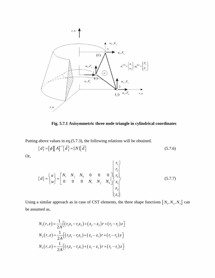
Fig. 5.7.1 Axisymmetric three node triangle in cylindrical coordinates

Putting above values in eq.(5.7.3), the following relations will be obtained.

[ ][ ] 1 [ ]d A d N dφ −= = (5.7.6)

Or,

1

2

3

1

2

3

0 0 00 0 0

i j k

i j k

rr

N N N rud

N N N zwzz

= =

(5.7.7)

Using a similar approach as in case of CST elements, the three shape functions [ ]1 2 3, ,N N N can

be assumed as,

( ) ( ) ( ) ( )

( ) ( ) ( ) ( )

( ) ( ) ( ) ( )

1 2 3 3 2 2 3 3 2

2 3 1 1 3 3 1 1 3

3 1 2 2 1 1 2 2 1

1,21,

21,

2

N r z r z r z z z r r r zA

N r z r z r z z z r r r zA

N r z r z r z z z r r r zA

= − + − + −

= − + − + −

= − + − + −

Or,

( ) ( )

( ) ( )

( ) ( )

1,21,

21,

2

i i i i

j j j j

k k k k

N r z r zA

N r z r zA

N r z r zA

α β γ

α β γ

α β γ

= + +

= + +

= + +

(5.7.8)

Where,

( )122

i j k k j j k i i k k i j j i

i j k j k i k i j

i k j i i k i j i

i j j k k i i k j i k j

r z r z r z r z r z r zz z z z z zr r r r r r

A r z r z r z r z r z r z

α α α

β β β

γ γ γ

= − = − = −

= − = − = −

= − = − = −

= + + − − −

(5.7.9)

Putting the value of u,w in eq. (5.7.7) from eq. (5.6.5),

[ ]

1

2

3

1

2

3

0 0 0

0 0 0

0 0 0

ji k

ji k

ji k

j ji k i k

NN Nrr r rrNN Nrr r r B dzNN Nzz z z

N NN N N N zz z z r r r

ε

∂ ∂ ∂ ∂ ∂ ∂ = = ∂∂ ∂ ∂ ∂ ∂ ∂ ∂∂ ∂ ∂ ∂ ∂ ∂ ∂ ∂ ∂ ∂

(5.7.10)

Thus, the strain displacement matrix can be expressed as,

[ ]

0 0 0

0 0 012 0 0 0

i j k

ji k

i j k

i j k i j k

NN NB r r r

A

β β β

γ γ γγ γ γ β β β

=

(5.7.11)

Where, 3

i j kr r rr

+ += . Thus the stiffness matrix will become

[ ] [ ] [ ][ ]Tk B D B d= Ω∫∫∫

Or, [ ] [ ] [ ][ ] [ ] [ ][ ]2

0

2T Tk B D B r d dA B D B r dr dzπ

θ π= =∫ ∫ ∫ ∫ ∫ (5.7.12)

Since, the term [B] is dependent of ‘r’ terms; the term [ ] [ ][ ]TB D B cannot be taken out of

integration. Yet, a reasonably accurate solution can be obtained by evaluating the [B] (denoted as [B]) matrix at the centroid.

Hence, [ ] [ ] [ ][ ]2 Tk r B D B dr dzπ= ∫ ∫

Or,

[ ] [ ] [ ][ ]2Tk B D B rAπ (5.7.13)

5.7.2 Stiffness Matrix of a Quadrilateral Element

50

The strain-displacement relation for axisymmetric problem derived earlier (eq.(5.6.5)) can be rewritten as

r

z

rz

ur

1 0 0 0 0 u0 0 0 1 0 z

w10 0 0 0 rrw0 1 1

urw

0 0z

zur

u wz r u

θ

εε

εεγ

∂∂ ∂ ∂ ∂ ∂ ∂ ∂= = = ∂

∂ ∂ ∂ ∂ + ∂

∂ ∂

(5.7.14)

Applying chain rule of differentiation equation we get,

* *11 12* *21 22

* *11 12* *21 22

uuξr

J J 0 0 0 uuηJ J 0 0 0z

w w0 0 J J 0rξ 0 0 J J 0w w0 0 0 0 1z η

u u

∂ ∂ ∂ ∂ ∂ ∂ ∂ ∂ =∂ ∂ ∂ ∂

∂ ∂ ∂ ∂

(5.7.15)

Hence, the strain components are calculated as

* *11 12

r * *21 22

z * *11 12

θ * *21 22

rz

uξ

J J 0 0 0 u1 0 0 0 0εηJ J 0 0 00 0 0 1 0εw0 0 J J 01ε 0 0 0 0 ξ0 0 J J 0r

0 1 1 0 0 w0 0 0 0 1η

u

γ

∂ ∂

∂ ∂ = ∂ ∂ ∂

∂

Or,

51

* *11 12

r * *21 22

z

* * * *rz21 22 11 12

u

uJ J 0 0 00 0 J J 0

w10 0 0 0r

wJ J J J 0

u

x h x h

(5.7.16)

With the use of interpolation function and nodal displacements, , , ,u u w wx h x h

can be expressed

for a four node quadrilateral element as

31 2 4

31 2 4

31 2 4

31 2 4

0 0 0 0

0 0 0 0

0 0 0 0

0 0 0 0

uNN N Nu

NN N Nu

w NN N N

w NN N N

x x x xx

h h h h h

x x x x x

h h h h h

1

2

3

4

1

2

3

4

uuuwwww

(5.7.17)

Putting eq. (5.7.17) in eq. (5.7.16) we get,

31 2 4

* *31 2 411 12

r * *21 22

z31 2 4

* * * *rz31 2 421 22 11 12

NN N N 0 0 0 0

NN N NJ J 0 0 0 0 0 0 00 0 J J 0

NN N N1 0 0 0 00 0 0 0r

NN N NJ J J J 0 0 0 0 0

x x x x

h h h h x x x x h h h

1

2

3

4

1

2

3

41 2 3 4 1 2 3 4

uuuuwwwwN N N N N N N N

h

(5.7.18) Thus, the strain displacement relationship matrix [B] becomes

52

31 2 4

* *31 2 411 12

* *21 22

31 2 4

* * * *31 2 421 22 11 12

1 2 3 4 1 2 3 4

NN N N 0 0 0 0

NN N NJ J 0 0 0 0 0 0 00 0 J J 0

B NN N N1 0 0 0 00 0 0 0r

NN N NJ J J J 0 0 0 0 0

N N N N N N N N

x x x x h h h h x x x x h h h h

(5.7.19)

For a four node quadrilateral element, ( ) 1 1

1

1ξ 1 η N N1η 1 ξN and 4ξ 4 η 4( ) ( ) ( )− − ∂ ∂− −

= ⇒ = − = −∂ ∂

( ) 2 12

1ξ 1 η N N1η 1 ξN and 4ξ 4 η 4( ) ( ) ( )+ − ∂ ∂− +

= ⇒ = = −∂ ∂

(5.7.20)

( ) 2 13

1ξ 1 η N N1η 1 ξN and 4ξ 4 η 4( ) ( ) ( )+ + ∂ ∂+ +

= ⇒ = =∂ ∂

( ) 2 14

1ξ 1 η N N1η 1 ξN and 4ξ 4 η 4( ) ( ) ( )− + ∂ ∂+ −

= ⇒ = − =∂ ∂

Thus, the [B] matrix will become

* *11 12

* *21 22

* * * *21 22 11 12

J J 0 0 00 0 J J 0

B 10 0 0 0r

J J J J 0

1 1 1 10 0 0 0

4 4 4 41 1 1 1

0 0 0 04 4 4 4

1 1 1 10 0 0 0

4 4 4 41 1 1 1

0 0 0 04 4 4 4

1 1 1 1 1 1 1 1 1 1 1 1 14 4 4 4 4 4

h h h h

x x x x

h h h h

x x x x

x h x h x h x h x h x h 1 1 14 4

x h x h (5.7.21) The stiffness matrix for the axisymmetric element finally can be found from the following expression after numerical integration.

[ ] [ ] [ ][ ] [ ] [ ][ ]1 1

T

1 1

B D B .2πr. .dξdηTk B D JB d+ +

Ω − −

= Ω =∫ ∫ ∫ (5.7.22)

53

Lecture 8: Finite Element Formulation for 3 Dimensional Elements 5.8.1 Introduction Solid elements can easily be formulated by the extension of the procedure followed for two dimensional solid elements. A domain in 3D can be discritized using tetrahedral or hexahedral elements. For example, the eight node solid brick element is analogous to the four node rectangular element. Regardless of the possible curvature of edges or number of nodes, the solid element can be mapped into the space of natural co-ordinates, i.e the 1,1,1 ±=±=±= ζηξ just like a plane element.

Fig. 5.8.1Eight node brick element For three dimensional cases, each node has three degrees of freedom having u, v, and w as displacement field in three perpendicular directions (X, Y and Z). In this case, one additional dimension increases the computational expense manifolds. 5.8.2 Strain Displacement Relation The strain vector for three dimensional cases can be written in the following form

54

1 0 0 0 0 0 0 0 00 0 0 0 1 0 0 0 00 0 0 0 0 0 0 0 10 1 0 1 0 0 0 0 00 0 0 0 0 1 0 1 00 0 1 0 0 0 1 0 0

x

y

z

xy

yz

zx

uxuyuzvxvyvzwxwywz

εεεγγγ

∂ ∂ ∂

∂ ∂

∂ ∂ ∂ ∂ = ∂

∂ ∂

∂ ∂ ∂

∂ ∂

∂ (5.8.1)

The following relation exists between the derivative operators in the global co-ordinates and the natural co-ordinate system by the use of chain rule of partial differentiation.

∂∂∂∂∂∂

∂∂

∂∂

∂∂

∂∂

∂∂

∂∂

∂∂

∂∂

∂∂

=

∂∂∂∂∂∂

z

y

x

zyx

zyx

zyx

ζζζ

ηηη

ξξξ

ζ

η

ξ

(5.8.2)

Where the Jacobian Matrix will be

[ ]

∂∂

∂∂

∂∂

∂∂

∂∂

∂∂

∂∂

∂∂

∂∂

=

ζζζ

ηηη

ξξξ

zyx

zyx

zyx

J (5.8.3)

For an isoparamatric element the coordinates at a point inside the element can be expressed by its nodal coordinate.

1 1 1and

n n n

i i i i i ii i i

x N x ; y N y z N z= = =

= = =∑ ∑ ∑ (5.8.4)

55

Substituting the above equations into the Jacobian matrix for an eight node brick element, we get

[ ]

∂∂

∂∂

∂∂

∂∂

∂∂

∂∂

∂∂

∂∂

∂∂

=∑=

ii

ii

ii

ii

ii

ii

ii

ii

ii

i

zNyNxN

zNyNxN

zNyNxN

J

ζζζ

ηηη

ξξξ8

1 (5.8.5)

The strain displacement relation is given by [ ] dB=ε , where,

=

wvu

d .

The displacements in the x, y and z direction are u, v, and w respectively. Let consider the inverse of Jacobian matrix as

[ ]

=−

*33

*32

*31

*23

*22

*21

*13

*12

*11

1

JJJJJJJJJ

J (5.8.6)

Thus, the relation between two coordinate systems can be rewritten as 1

11 12 13

21 22 23

31 32 33

* * *

* * *

* * *

x y zx J J J

x y z J J Jy

J J Jx y z

z

ξ ξ ξ ξ ξ

η η η η η

ζ ζ ζ ζ ζ

− ∂ ∂ ∂ ∂ ∂ ∂ ∂ ∂ ∂ ∂ ∂∂ ∂ ∂ ∂ ∂ ∂ ∂ = = ∂ ∂ ∂ ∂ ∂ ∂ ∂ ∂ ∂ ∂ ∂∂

∂ ∂ ∂ ∂ ∂∂

(5.8.7)

Thus, one can write the following relations

8 8

11 12 13 11 12 131 1

* * * * * *i i ii i i

i i

N N Nu u u uJ J J J J J u a ux ξ η ζ ξ η ζ= =

∂ ∂ ∂ ∂ ∂ ∂ ∂= + + = + + = ∂ ∂ ∂ ∂ ∂ ∂ ∂

∑ ∑

8 8

21 22 23 21 22 231 1

* * * * * *i i ii i i

i i

N N Nu u u uJ J J J J J u b uy ξ η ζ ξ η ζ= =

∂ ∂ ∂ ∂ ∂ ∂ ∂= + + = + + = ∂ ∂ ∂ ∂ ∂ ∂ ∂

∑ ∑

8 8

31 32 33 31 32 331 1

* * * * * *i i ii i i

i i

N N Nu u u uJ J J J J J u c uz ξ η ζ ξ η ζ= =

∂ ∂ ∂ ∂ ∂ ∂ ∂= + + = + + = ∂ ∂ ∂ ∂ ∂ ∂ ∂

∑ ∑

Similarly, 8 8 8 8 8 8

1 1 1 1 1 1andi i i i i i i i i i i i

i i i i i i

v v v w w wa v ; b v ; c v ; a w ; b w c wx y z x y z= = = = = =

∂ ∂ ∂ ∂ ∂ ∂= = = = = =

∂ ∂ ∂ ∂ ∂ ∂∑ ∑ ∑ ∑ ∑ ∑

Using above relations, the strain vector can be written as

56

8

1

0 00 00 0

00

0

x i

y ii

z ii

ixy i ii

yz i i

zx i i

uxv

aybw u

cz vu v b a

wy x c bv w c az yu wz x

εεε

εγγγ

=

∂ ∂

∂ ∂

∂ ∂ = = = ∂ ∂ + ∂ ∂ ∂ ∂ +

∂ ∂ ∂ ∂ + ∂ ∂

∑ (5.8.8)

Now, the strain displacement relationship matrix [B] can be identified from the above equation by

comparing it to [ ] dB=ε . 5.8.3 Element Stiffness Matrix The element stiffness matrix can be generated similar to two dimensional case using the following relations.

[ ]1 1 1

1 1 1

Tk [ B ] [ D ][ B ]d d d Jξ η ζ+ + +

− − −

= ∫ ∫ ∫ (5.8.9)

The size of the constitutive matrix [D] for solid element will be 6 × 6 and is already discussed in module 1, lectures 3. For eight node brick element, the size of stiffness matrix will become 24 × 24 as number of nodes in one element is 8 and the degrees of freedom at each node is 3. It is well established that 2 × 2 × 2 Gauss integration points are the optimal sampling points for eight node isoparametric brick elements.

5.8.4 Element Load Vector The forces on an element can be generated due to its self weight or externally applied force which may be concentrated or distributed in nature. The distributed load may be uniform or non-uniform. All these types of loads are to redistributed to the nodes using finite element formulation.

5.8.4.1 Gravity load The load vector due to body forces in general is given by

TQ [ N ] X dΩ

= Ω∫ (5.8.10)

57

where X is the body forces per unit volume. The nodal load vector at any node i may be expressed as

Ti iQ [ N ] X d

Ω

= Ω∫ (5.8.11)

In case of gravity load, the force will act in the global negative Z direction. Therefore,

=

i

i

i

i

NN

NN

000000

][ and 00X

gρ

= −

(5.8.12)

Here, the mass density of the material is ρ and the acceleration due to gravity is g. Thus, eq.(5.8.11) will become

00i

i

Q dN gρΩ

= Ω − ∫ (5.8.13)

For isoparametric element the, the above expression will become

ζηξρ

dddJN

Q

i

i ∫ ∫ ∫+

−

+

−

+

−

−=

1

1

1

1

1

100

(5.8.14)

Using Gauss Quadrature integration rule, the above expression may be evaluated as

1 1 1

00

i j k

n n n

i i j k i j ki j k

i ( , , )

Q w w w J ( , , )N g

ξ η ζ

ξ η ζρ= = =

= −

∑∑∑ (5.8.15)

Where, n is the number of nodes in an element. For eight node linear brick element the value of n will be 8 and the integration order suggested is 2×2×2. Similarly, for twenty node quadratic brick element, the value of n will be 20 and the integration order suggested is 3×3×3.

5.8.4.2 Surface pressure Let assume a uniform surface pressure of intensity q is acting normal to the element face. The load vector due to surface pressure is given by

∫∫= dApNQ Ts ][ (5.8.16)

The nodal load at any node i may be expressed as ∫∫= dApNQ Ts

ii ][ (5.8.17)

In case of surface load, the value of ][ siN in the above equation will become

58

=si

si

si

si

NN

NN

000000

][ (5.8.18)

Here siN is the interpolation function for the node i. For example, the value of s

iN can be obtained

by substituting ξ =1 in siN for face 1. Thus, the surface pressure is expressed as,

=

3

3

3

qnqmql

p (5.8.19)

Where, 333 ,, nml are the direction cosines. Thus, eq.(5.8.17) can be expressed using eq.(5.8.19) in the following form.

dAqnNqmNqlN

Qsi

si

si

i ∫ ∫+

−

+

−

=1

1

1

1

3

3

3

(5.8.20)

The value of dA is can be evaluated considering the cross product of vectors along the natural coordinates parallel to the loaded faces of the element. Thus,

ζηddeedA 32 ×= (5.8.21)

5.8.5 Stress Computation Using the relation of F = [K]d, the unknown nodal displacement vector d are calculated in global coordinate system. Once the nodal displacements are obtained, the strain components as each node can be computed using strain-displacement relations for each element. Similarly element stress can be calculated using stress-strain relation. These stresses at Gauss points are extrapolated to the corresponding nodes of the element to find the nodal stresses. In general, for three dimensional state of stress there are at least three planes, called principal planes. The corresponding stress vector is perpendicular to the plane and where there are no normal shear stresses. These three stresses which are normal to these principal planes are called principal stresses. The principal stresses σ1, σ2, and σ3 are computed from the roots of the cubic equation represented by the determinant of the flowing.

0x xy xz

xy y yz

xz yz z

σ σ τ ττ σ σ ττ τ σ σ

−− =

− (5.8.22)

The characteristic equation has three real roots σi, due to the symmetry of the stress tensor. The principal stresses are arranged so that σ1 > σ2 > σ3. The maximum shear stress can be computed from the following relations.

59

1 2 2 3 3 1max = largest of and

2 2 2,

σ σ σ σ σ στ

− − −

(5.8.23)

These three shear stress components will occur on planes oriented at 450 from the principal planes. The distortion energy theory suggests that the total strain energy can be divided into two components. They are (i) volumetric strain energy and (ii) distortion or shear strain energy. It is anticipated that yield develops if the distortion component exceeds that at the yield point for a simple tensile test. From the concept of distortion energy theory, the equivalent stress which is historically known as Von Mises stress are defined as

( ) ( ) ( )2 2 21 2 2 3 3 1=

2e

σ σ σ σ σ σσ

− + − + −

(5.8.24)

The Von Mises stresses offer a measure of the shear or distortional stress in the material. In general, this type of stress tends to cause yielding in metals.

60

Worked out Examples Example 5.1 Calculation of nodal loads on a triangular element A CST element as shown in Fig. 5.I gets axial loading of (Fx1) 10 kN/m in X direction and (Fy1) 20 kN/m in Y direction. Compute the nodal loads in the element.

Fig. 5.I Distributed loading on a triangular element

From the above figure, the length of sides 1, 2 and 3 are calculated and will be 10, 8 and 6 cm respectively. First, let consider side 1:

[ ] 1

10

lTF N F dsΓ= ∫

Or,

1 1 1

2 2 2

13 3 31

10 0 0

2 2

3 3

0 0 0 0 00 00 0 10

100 0 0 0 0 00 0 00 0 0

l l lx

y

L L LFL L L

F ds ds dsF

L LL L

= = = ×

∫ ∫ ∫

Putting, ( )1 2

! !1 !

p q p qL L ds lp q

=+ +∫ , we will get,

61

11

0 0 01 1 0.51 1 0.50.110 100 0 02 20 0 00 0 0

lF

= × × = × × =

Similarly for side 2,

2 2

1 1

23 3 22

21 10 0

3 3

0 0 0 00 0 0 0 0 0

0 0 0 0 020

0 0 20 1 0.820 0 0 0 0 00 0 1 0.8

l lx

y

L L

FL L lF ds ds kNFL L

L L

= = = × × =

∫ ∫

Since no force is acting on side 3,

3

000000

F

=

Hence, the nodal load vector in all the nodes in x and y directions will become,

00.50.50.80

0.8

F

=

kN.