i

NOVEL SCHEME FOR ANALYSING THE NOISE LIMITATIONS OF

AVERAGE AND GUIDED SOLITON COMMUNICATION SYSTEMS

ZAHARIAH BINTI ZAKARIA

A thesis submitted in

fulfillment of the requirement for the award of the

Doctor of Philosophy

Faculty of Science, Technology and Human Development

Universiti Tun Hussein Onn Malaysia

JANUARY 2013

v

ABSTRACT

This thesis presents analytical and numerical investigations of optical soliton

transmission in optical fibre communication systems. The basic principles of

nonlinear pulse propagation in optical fibre are discussed followed by discussion of

the main limitations for an amplified soliton based system. The goal of this work is to

study in-depth the soliton propagation and to analyse the bit pattern noise analysis and

multi-slot analysis of system performance. First, a performance comparison of

mqocss, VPI and OptSim for single and WDM transmission systems is presented. The

purpose of this comparison is to assess the degree of variability between

independently written numerical simulation codes and the commercial software

available in the market. Secondly, a study of average soliton systems with 35, 50 and

70 km amplifier spacing is presented both analytically and numerically. The

effect of modifying the existing rule of thumb formulae is presented in terms of a

design diagram. This is then compared to the numerical simulations. The introduction

of optimum jitter parameter, αsq = 0.05 in the formulation of GH limitation and

optimum ratio of Belec to Bopt, BRAT = 0.4, of the ASE limitation improve the better

comparison between analytical and numerical results. A series of design diagram with

Gordon-Haus (GH) jitter, signal to noise ratio (SNR) and soliton collapse limited

transmission is also introduced. The same study has been repeated for guided soliton

systems. Finally a significant portion of this work is devoted to the noise analysis of

GH and SNR limited system transmission. A novel technique is introduced which is

designed to distinguish between the effects of dispersion and jitter in analysing the

limitations of system performance. These are represented in the form of probability

distribution function on amplitude and timing jitter, by introducing the two methods

(A and B), referring to the eye diagrams of the system limitations. Another technique

analysis is presenting the energy plots of En+1 and En-1, the energy adjacent to bit

under consideration. The plot also explains the limitation due to amplified soliton,

ASL.

Key words: Optical amplification, Guiding Centre Soliton, Guided Soliton, GH and

SNR limited transmission, Noise analysis.

vi

ABSTRAK

Tesis ini membentangkan penyelidikan secara analitik dan numerik bagi penghantaran

„soliton‟ optik di dalam sistem komunikasi gentian optik. Prinsip asas perambatan

denyut tak linear dalam gentian optik akan dibincangkan diikuti dengan perbincangan

had-had perambatan bagi sistem soliton yg diamplifikasikan. Objektif kajian ini

adalah untuk mendalami perambatan soliton seterusnya menganalisis prestasi sistem

pada corak hingar untuk setiap „bit‟ dan „multi bit‟. Perkara pertama yang

dibincangkan ialah perbandingan dari segi prestasi di antara mqocss, VPI and OptSim

bagi sistem penghantaran tunggal dan sistem penghantaran WDM. Tujuan

perbandingan ini ialah untuk menilai darjah kebolehubahan di antara kod

pengaturcaraan dan perisian komersil. Kedua, kajian tentang sistem “average

soliton”. Reka bentuk sistem dan hasil dapatan pada jarak penguat 35, 50 dan 70 km

(yang membentuk keseluruhan jarak 3500 km) akan di bincangkan secara analitik dan

numerik termasuk kesan mengubah parameter-parameter kepada formula sedia ada.

Pengenalan kepada nilai optimum “jitter” , αsq = 0.05 dalam formulasi had GH dan

nilai optimum nisbah Belec to Bopt , BRAT = 0.4 pada had ASE menambah baik

perbandingan antara output analitik dan numerik. Di bahagian ini juga diperkenalkan

gambarajah rekabentuk sistem penghantaran yang terhad kepada Gordon Haus (GH),

nisbah isyarat-hingar (SNR) dan „keruntuhan‟ soliton. Kajian serupa juga dibuat untuk

“guided soliton” dan analisis yang sama diulang untuk sistem ini. Akhirnya bahagian

terpenting ditumpukan kepada analisis hingar sistem penghantaran yang dihadkan

oleh GH and SNR. Satu teknik baru diperkenalkan untuk membezakan di antara

kesan-kesan “dispersion” dan “jitter” dalam menganalisis prestasi bagi sistem

tersebut. Analisis yang dilakukan adalah dalam bentuk fungsi taburan kebarangkalian

pada amplitud dan masa, dengan memperkenalkan dua cara (A dan B) merujuk kepada

bentuk “eye diagram” bagi setiap had system. Teknik lain ialah mempamerkan plot

tenaga di En+1 and En-1, iaitu tenaga bersebelahan “bit” yang dikaji. Plot tenaga ini

juga boleh menerangkan had yang disebabkan oleh soliton yang dikuatkan, ASL.

Perkataan kunci: Penguatan optik, Guiding Centre Soliton, Guided Soliton,

Penghantaran terhad GH dan SNR, analisis hingar.

vii

CONTENTS

TITLE i

DECLARATION ii

DEDICATION iii

ACKNOWLEDGEMENT iv

ABSTRACT v

CONTENTS vii

LIST OF FIGURES xii

LIST OF ABBREVIATIONS xviii

CHAPTER 1 INTRODUCTION TO FIBRE-OPTIC TRANSMISSION 1

1.1 Historical perspective of fibre optic communication

system 1

1.2 Solitons in optical communication systems 3

1.3 Objectives of Study

1.4 Problem Statement

1.5 Scope and Delimitation

1.6 Chapter overview 4

viii

CHAPTER 2 PULSE PROPAGATION IN OPTICAL FIBRES 6

2.1 Basic propagation equation 6

2.1.1 Pulse propagation governed by GVD 10

2.1.2 Pulse propagation governed by SPM 16

2.1.3 Pulse propagation governed by GVD and SPM 18

2.2 Optical solitons: characteristics and conditions for Propagation 20

2.2.1 Fundamental and higher order solitons 21

2.2.2 Interaction between solitons 22

2.3 Summary 24

CHAPTER 3 AMPLIFIED SOLITON SYSTEMS 25

3.1 Characteristics and limiting factors from optical fibre 25

3.1.1 Fibre losses 25

3.1.2 Chromatic dispersion 27

3.1.3 Nonlinearity 28

3.2 Characteristics and limiting factors from Erbium-doped

fibre amplifiers (EDFAs) 29

3.2.1 The average soliton 31

3.3 Main limitations for an amplified soliton 33

3.3.1 Gordon Haus, GH effects 33

3.3.2 Amplified Spontaneous Emission, ASE Noise

Accumulation 36

3.3.3 Periodic attenuation and amplification of the solitons 37

3.3.4 Interaction between solitons (soliton collapse) 38

ix

3.4 Concept of design Diagrams 38

3.5 Characterisation of System Performance 40

CHAPTER 4 COMPARISON OF NUMERICAL SIMULATION

SOFTWARE 44

4.1 Basic Concepts 44

4.1.1 Signal and Bit Patterns 44

4.1.2 Gaussian Pulse 45

4.1.3 Modulation Format 45

4.2 Optical Communication System Components 46

4.2.1 Optical Channel 46

4.2.2 Optical Transmitter 46

4.2.3 Optical Receiver 47

4.3 System Performance 48

4.3.1 Bit Error Rate and Q-factor 48

4.3.2 Fibre Loss and Fibre Dispersion 48

4.4 System Simulation 49

4.5 Commands Used for Fibre-Optic Simulation in XML 49

4.6 Propagation of a Single Pulse in Fibre 52

4.6.1 The XML Configuration File for Single Pulse

Propagation 53

4.6.1.1 Result of Propagation of a Single Pulse in Mqocss 53

4.6.2 VPI in Windows System 54

4.6.2.1 How to start VPItransmissionMaker? 54

4.6.2.2 Setting Parameters 56

4.6.2.3 Running the Simulations 57

4.6.2.4 Result of Propagation of a Single Pulse in VPI 57

4.6.3 OptSim in Windows System 59

4.6.3.1 How to Start OptSim in Windows System 59

4.6.3.2 To Create a New Project 60

4.6.3.3 Drawing the Schematic 61

4.6.3.4 Exporting a Design 61

4.6.3.5 Running the Simulation 62

4.6.3.6 Using the Data Display 63

4.6.3.8 Observation 65

4.6.4 Conclusion for Simple Dispersion 67

x

4.7 Transmission of a Single System 67

4.7.1 The XML Configuration File of Single Transmission

System 68

4.7.2 Simulation Using VPI 69

4.7.3 Performance comparison of power and Q-factor for

mqocss and VPI 70

4.7.4 Simulation Using OptSim 72

4.7.4.1 Result of single transmission system in OptSim 72

4.7.5 Discussion and Conclusion 73

CHAPTER 5 AVERAGE SOLITON SYSTEM 75

5.1 Effects on changing the system parameters in the design

diagram 76

5.2 Numerical simulations and system parameters 82

5.3 Analytical analysis 84

5.4 Analytical model and limitations on the design diagram 86

5.5 Effect of changing BRAT and jitter term to the design

Diagram 91

5.6 Conclusion 94

CHAPTER 6 GUIDED SOLITON SYSTEM 96

6.1 Soliton transmission control 97

6.2 System performance 98

6.3 Analytical simulation 99

6.4 Numerical simulation 104

6.5 Conclusion 109

xi

CHAPTER 7 BIT PATTERN NOISE ANALYSIS 111

7.1 Receiver design 112

7.2 Numerical simulations 113

7.3 Probability distribution function and pulse arrival time 114

7.4 Average soliton system 116

7.5 Guided soliton system 118

7.6 Conclusion 120

CHAPTER 8 MULTI-SLOT ANALYSIS OF SYSTEM PERFORMANCE 121

8.1 Energy distribution in bit slots 121

8.2 Pattern dependence of noise properties 124

8.3 Noise analysis in PRBS pattern 128

8.3.1 SNR limited system at 1200 km 128

8.3.2 ASL limited system at 1200 km 129

8.3.3 SNR and GH limited system at 3500 km 131

CONCLUSION 133

Appendix 1 136

Reference 137

xii

LIST OF FIGURES

2.1 A plot of normalized pulsewidth vs normalized distance for

Different Gaussian pulses with initial width=1,3 and 5 (for 12 ) 13

2.2 Broadening factor for a chirped Gaussian pulse as a function

distance for unchirped Gaussian pulse, positive and negative chirp 14

2.3 Variation of the dispersion parameter D with wavelength for a

standard monomode fibre showing that zero dispersion at m 3.1 15

2.4 Anomalous and normal dispersion regimes 15

2.5 Amplitude of 1st and 4th order Gaussian pulses with time 17

2.6 Induced chirp caused by phase changes across 1st and 4th order

Gaussian pulses 18

2.7 Evolution of pulse shapes over a distance z/LD for an initially

unchirped Gaussian pulse propagating in the normal dispersion

regime of the fibre.(After ref. Agrawal G.P,2001) 20

2.8 Evolution of pulse shapes over a distance z/LD for an initially

unchirped Gaussian pulse propagating in the anomalous dispersion

regime of the fibre. (After ref. Agrawal G.P,2001) 20

2.9 Amplitude versus time for different soliton separations and phase

differences 23

2.10 Evolution of soliton pair showing the effects of soliton interaction

for amplitude ratio 1 and relative phase 0 and 4

(After ref Agrawal G.P,2001) 24

3.1 Loss profile of a single mode fibre (After ref Senior J.M 1992) 26

3.2 Energy diagram of Er3+-ions in glass hosts 29

3.3 Loss and amplification of soliton during propagation over 4 amplifier

spans.The soliton average power is shown by the dotted line 32

xiii

3.4 Schematic of timing jitter origin 34

3.5 Fibre links with periodic loss compensation through

optical N amplifiers 39

3.6 Soliton design diagram for 3500 km system length for (a) average soliton

and (b) guided soliton 40

3.7 Bit Error Rate versus Q factor 42

4.1 Digital bit stream 01010…coded by using RZ and NRZ formats 46

4.2 Components of optical transmitter 47

4.3 Components of an optical receiver 48

4.4 The input and output peak power over time for mqocss 54

4.5 Login Window for VPI 54

4.6 A set-up design for task 1 in VPI 55

4.7 Schematic Diagram for VPI 55

4.8 Simulation Job Window 57

4.9 A plot of power vs time for VPI 58

4.10 Comparison of input and output peak power over time for VPI

and mqocss 58

4.11 OptSim Startup Dialog 59

4.12 The Simulation Parameters dialog window – Basic Attributes section 60

4.13 OptSim Editor window 61

4.14 Export windows 62

4.15 Variable Bandwidth Simulation options 63

4.16 The Measurement List Window 64

4.17 Measurement Window 64

4.18 Schematic Design for example 1 65

4.19 A plot of power in mW with time in ps for input file 66

4.20 A plot of power in mW with time in ps for output file 66

xiv

4.21 Comparison of input and output peak power over time for OptSim

and mqocss 67

4.22 Set-up Diagram in VPI for Task 2 70

4.23: (a) Performance Comparison in power and Q-parametres for mqocss

and VPI for 0.06 ps/km/nm2 3

rd order dispersion and

(b) in a smaller scale of Q 71

4.24 Set-up Diagram in OptSim for Task 2 72

4.25 Power and Q-parameter over the Length of Fibre for several

runs in VPI 73

5.1 a. Variation of pulsewidth with amplifier spacing for

propagation distance=1000 km 77

5.1 b. Variation of pulsewidth with amplifier spacing for propagation

distance=2000 km 77

5.1 c. Variation of pulsewidth with amplifier spacing for propagation

distance=3000 km 78

5.1 d. Variation of pulsewidth with amplifier spacing for propagation

distance=4000 km 78

5.1 e. Variation of pulsewidth with amplifier spacing for Lt=10000 km

- no intersection! There is where there is no combination of system parameters

that satisfies all the criteria 79

5.2 a. Variation of pulsewidth with amplifier spacing

for bitrate = 5 Gbit/s 80

5.2 b. Variation of pulsewidth with amplifier spacing

for bitrate = 10 Gbit/s 80

5.2 c. Variation of pulsewidth with amplifier spacing

for bitrate = 15 Gbit/s 81

5.2 d. Variation of pulsewidth with amplifier spacing

for bitrate = 20 Gbit/s 81

5.3 a. Plot of pulsewidth versus dispersion numerical simulation

with La=35 km 83

5.3 b. Plot of pulsewidth versus dispersion numerical simulation

with La=50 km 83

5.3 c. Plot of pulsewidth versus dispersion numerical simulation

with La=70 km 84

xv

5.4 a. Analytical plot with its limitations at La=35 km 85

5.4 b. Analytical plot with its limitations at La=50 km 85

5.4 c. Analytical plot with its limitations at La=70 km 86

5.5 a. Numerical and analytical plot of pulsewidth versus dispersion

for La=35km 87

5.5 b. Numerical and analytical plot of pulsewidth versus dispersion

for La=50 km 88

5.5 c. Numerical and analytical plot of pulsewidth versus dispersion

for La=70 km 88

5.6 a. Eyediagrams at La=50 km for dispersion, D=0.2 at different

position in a pulsewidth versus dispersion plot 90

5.6 b. Eyediagrams at La=50 km for dispersion, D=1 at different

position in a pulsewidth versus dispersion plot 90

5.7 A plot of pulsewidth with dispersion for different BRAT 91

5.8 A plot pulsewidth with dispersion for different jitter 92

5.9 a. Numerical and analytical plot showing the variation of

pulsewidth over dispersion for a different jitter at La=35 km 92

5.9 b. Numerical and analytical plot showing the variation of

pulsewidth over dispersion for a different jitter at La=50 km 93

5.9 c. Numerical and analytical plot showing the variation of

pulsewidth over dispersion for a different jitter at La=70 km 93

5.10 a. Analytical plot for pulsewidth versus dispersion for

different amplifier spacings 94

5.10 b. Numerical plot for pulsewidth versus dispersion for

different amplifier spacings 94

6.1 Relationship between eye-opening and Q-factor.(after ref. [4] 98

6.2 Q factor as a function of pulsewidth, for a system with and

without in-line filter 99

6.3 A plot of factor f(x), (equation 6.4) for GH jitter due to in-line

filtering 100

xvi

6.4 A plot of pulsewidth versus amplifier spacing at distance,

L=1500km, D=0.5ps/km nm, T=20ps (a) no filter (b) with filter 101

6.5 A plot of pulsewidth versus amplifier spacing at distance,

L=4500km, D=0.5ps/km nm, T=20ps (a) no filter (b) with filter 102

6.6 Analytical plot of pulsewidth versus dispersion for different

amplifier spacing. a. La = 35 km, b. La = 50 km, c. La = 70 km 103

6.7 Monitoring average signals with distance during soliton

Propagation 105

6.8 Eye diagram of received solitons in the presence of spontaneous

emission noise-GH effect 106

6.9 Eye diagrams of received solitons in the presence of spontaneous

emission noise reduced by in-line filter 106

6.10 Numerical plots of pulsewidth versus dispersion for a system with

and without inline filters at 3 different amplifier spacings:

a. La = 35 km, b. La = 50 km, c. La = 70 km 107

6.11 Comparison between numerical and analytical plot for a system

with inline filters at 3 different amplifier spacings:

a. 35 km b. 50 km c. 70 km 108

7.1 Block diagram of an optical receiver (after ref. [5],[6] ) 113

7.2 Eye diagram (power in mW versus time in ps) for average soliton

(a) GH limited system (b) SNR limited system at 3500 km

(70 amplifiers) 114

7.3 Eye diagram (power in mW versus time in ps) for guided soliton

(a) GH/ASL limited system (b) SNR limited system at 3500 km

(70 amplifiers) 114

7.4 Amplitude PDF as a function of power for GH limited transmission

in an average soliton system 116

7.5 Amplitude PDF as a function of power for SNR limited transmission

in an average soliton system 117

7.6 Amplitude PDF as a function of time for GH and SNR limited

transmission in an average soliton system analysed using method B 117

7.7 Amplitude PDF as a function of power for ASL limited transmission in a

guided soliton system 118

7.8 Amplitude PDF as a function of power for SNR limited transmission

in a guided soliton system 119

xvii

7.9 Amplitude PDF as a function of time for GH and SNR limited

transmission in guided soliton system analysed using method B 120

8.1 Soliton pulse in a slot with noise in the neighboring slots 122

8.2 Soliton energy (exaggerated) in a slot with noise in the

neighbouring slots 122

8.3 Soliton pulse is broadened due to dispersion 123

8.4 Energy distributions in slots adjacent to a soliton due to dispersion 123

8.5 Soliton pulse is shifted due to timing jitter 123

8.6 Energy distributions in slots adjacent to a soliton due to timing jitter 124

8.7 Eye diagram for GH limited system at D=0.8 ps/km/nm 126

8.8 The plots of energies for GH limited system 126

8.9 Eye diagram for GH limited system at D=0.17 ps/km/nm 127

8.10 The plots of energies for a GH limited system 127

8.11 Eye diagram for SNR limited system at D=0.17 ps/km/nm 127

8.12 The plots of energies for SNR limited system 128

8.13 a, b Plots of En+1 against En-1 for SNR limited case at 1200 km 129

8.14 Plot of energy En+1 against En-1 for ASL (for D=0.1 ps /km nm)

at 1200 km 130

8.15 Eye diagram for ASL at D=0.1 ps/km nm. The green curve shows the eye

diagram at 50 km after the loop of amplifier 130

8.16 (a) plot of energies and (b) eye diagram for GH limited system

at D=1 ps/ km nm 131

8.17 SNR limited system at 3500 km 131

8.18 GH limited system at 3500 km 133

8.19 SNR and GH limited system at (a) 1200 km and (b) 3500 km 133

xviii

LIST OF ABBREVIATIONS

ASE Amplified Spontaneous Emission

ASL Average Soliton Limit

BER Bit Error Rate

BRAT Bandwidth Ratio

BW Bandwidth

CW Continuous Wave

DCF Dispersion Compensating Fibre

DSF Dispersion Shifted Fibre

EDFA Erbium Doped Fibre Amplifier

FBG Fibre Bragg Grating

FWHM Full Width Half Maximum

FWM Four Wave Mixing

GH Gordon-Haus

GVD Group Velocity Delay

NF Noise Figure

NLSE Non-Linear Schrödinger Equation

NRZ Non Return to Zero

OSNR Optical Signal to Noise Ratio

PDF Probability Distribution Function

RZ Return to Zero

SBS Stimulated/Spontaneous Brillouin Scattering

SC Soliton Collapse

SMF Single Mode Fibre

SNR Signal to Noise Ratio

SPM Self Phase Modulation

SRS Stimulated/Spontaneous Raman Scattering

WDM Wavelength Division Multiplexing/Multiplexer

XPM Cross Phase Modulation

1

CHAPTER 1

INTRODUCTION TO FIBRE-OPTIC TRANSMISSION

1.1 Historical perspective of fibre optic communication system

The rapid progress of optical communications is basically stimulated by the

continuous increase in the demand for telecommunication services. Researchers and

designers of optical networks live in a permanent quest for new techniques to augment

the capacity and flexibility of the existing communications systems/networks, and also

for the development of new concepts to meet the requirements of long distance and/or

high capacity transmission systems. Optical communication has been proven to be the

only reasonable choice to meet such a demanding requirement (Senior J.M., 1992).

Optical fibre can transmit ultra high speed information with extremely low loss over a

wide range of wavelengths. By virtue of this outstanding property, fibre-optic

communication technologies have been applied to a variety of transmission systems

throughout the world, such as international undersea networks and terrestrial links

(Agrawal G.P., 2002).

In the early 1960s the idea of optical waves for communications was faced

with two main problems; those were the availability of a suitable source of such waves

and the need for a suitable medium of transmission delayed the progress. Both

problems were solved by the invention of lasers in 1960 and the availability of GaAs

semiconductor lasers in 1970, the first proposal of glass fibre and the subsequent

development of low loss glass fibre that can guide the optical waves over long

distances (Senior J.M., 1992). An optical communication system based on a single

mode fiber transmitted 2 Gb/s over 40 km in 1981 (Yamada J. I., Kimura T., 1981).

The communication technology has shown rapid progress since then. In just 20 years

the bit rates have increased to 40 Gb/s and more. Below is the summary of time line

2

on progress and development of fibre optic communication systems (Mollenauer L.F.,

1986, Mollenauer L.F., 1988, Mollenauer L.F, S.G.E, Haus H.A., 1991, Hasegawa A,

Kodama Y., 1990, Hasegawa A., Kodama Y., 1991).

1960: Invention of the laser

1970: The first optical fibre was fabricated, with losses of 20 dB/km, and

operating in the region of 1 m

1978: Commercial operation of the first generation of optical communication

systems

- multimode fibres, near 0.8 m

- up to 10 km spacing between repeaters

- bit rates around 45 Mb/s

Beginning of the 80‟s: Second generation of optical communication systems

- multimode fibres, near 1.3 m

- up to 20 km spacing between repeaters

- bit rates around 100 Mb/s

1987: Commercial operation of the second generation of optical

communication systems

- monomode fibres, near 1.3 m

- up to 50 km spacing between repeaters

- bit rates around 1.7 Gb/s

Second of the 80‟s: third generation of optical communication systems

- monomode fibres, near 1.55 m

- 60-70 km spacing between repeaters

- no improvement on bit rate

End of the 80‟s: development of EDFA‟s

- reduced coupling losses

- amplification process: stimulated emission

- 30 dB gain

- low pump powers: 30 mW

Beginning of the 90‟s: commercial operation of the third generation of optical

communication systems, with bit rates around 2.5 Gb/s, and deploying

EDFA‟s

Mid 90‟s: modern optical communication systems of the fourth generation

- EDFA‟s

- coherent detection

WDM technology

- terrestrial and submarine transmissions

Suggestion and development of dispersion compensation techniques

- motivation for the fifth generation of optical communication

systems, based on optical solitons

3

1.2 Solitons in optical communication

Solitons have been studied in many fields of science; however, the most promising

applications of soliton theory are in the field of optical communications. In such

systems information is encoded into light pulses and transmitted through optical fibers

over large distances. Optical communication systems are no longer the pipedreams of

the future. Commercial systems have been in operation since 1977. The transatlantic

undersea optical cable has been developed, which is expected to transmit around

40,000 telephone conversations simultaneously. The development of optical fibres,

which are the basis of such systems, has lead to a revolution in communications

technology.

In 1973 Hasegawa and Tappert proposed that soliton pulses could be used in

optical communications through the balance of nonlinearity and dispersion. They

showed that these solitons would propagate according to the nonlinear Schrodinger

equation (NLSE), which had been solved by the inverse scattering method a year

earlier by Zakharov and Shabat. At that time there was no capability to produce the

fibres with the proper characteristics for doing this and the dispersive properties of

optical fibres were not known. Also, the system required a laser which could produce

very short pulse widths, which also was unavailable. Mollenauer, Stollen and Gordon

(1985, 1986, 1988, 1991) at AT&T Bell Laboratories then experimentally

demonstrated the propagation of solitons in optical fibers.

The original communications systems employed pulse trains with pulse widths

of about one nanosecond. However, there was still some distortion due to fibre loss.

This was corrected by placing electronic repeaters every several tens of kilometres. In

the mid 1980's it was proposed that by sending in an additional pump wave along the

fibre, the fibre loss could be compensated through a process known as Raman

scattering. In 1988, Mollenauer and his group showed that this could indeed be done

by propagating a soliton over 4000 km without the need for electronic repeaters. This

was one of the first demonstrations of an all-optical transmission system. Such

systems became even more common with the development of the Erbium amplifier.

4

Below is a summary of the time line on significant progress and development of

solitons in optical communication systems.

1838: observation of solitary waves in water

1895: mathematical description – KdV equation

1972: optical solitons as solutions to the NLSE

1973: dispersion and nonlinear phenomena

1980: experimental demonstration on propagation of soliton in optical fibres

by Mollenauer, Stolen and Gordon. This is followed by extensive experiments

conducted by the group at Bell Laboratories and confirmed the predictions of

nonlinear Schrödinger equation.

1986: The analysis of nonlinear effect (Gordon-Haus effect) by Haus H. A

and Gordon J. P when ASE noise from amplifiers is considered in the system.

1990: EDFAs –pioneering work in the development of diode-pumped

Erbium-doped amplifiers by Desurvive, Mears, Tachibana, Zynskind

(worldwide)

90‟s: soliton control techniques for example sliding guiding filter concept

introduced by Gordon et al 1992, Mollenauer et al. 1993, in an attempt to push

the transmission capacity to a higher limits.

1998: 40 channel WDM, combining optical solitons of different wavelengths,

demonstrated a data transmission of 1 terabit per second (1,000,000,000,000

units of information per second).

2001: the practical use of solitons deployed submarine telecommunications

equipment in Europe carrying real traffic using John Scott Russell's solitary

wave.

1.3 Objectives of Study

Analytical and numerical investigations of an optical soliton transmission in

optical fibre communication systems are studied. Specifically the main aim of this

work is to analyse the noise resulted from this study with the following objectives:

1. To investigate the soliton propagation in fibre optics.

5

2. To model the propagation of soliton in fibre optics with the use of non-linear

Schrödinger equation.

3. To numerically simulate the systems.

4. To compare and contrast the output between the analytical and the numerical

simulations.

5. To perform analysis on the noise in the system used.

In general, these objectives have been achieved using two soliton systems namely

the guiding centre soliton and the guided soliton which will be elaborated in

chapter 5 and 6, respectively.

1.4 Problem Statement

In designing a soliton transmission system, there are several effects which

must be taken into consideration. The design of the system depends not only on

the system length but also on the data rate and amplifier span which are required.

As shall be seen there must be compromises made in the system design brought

about by the requirements of low timing jitter on arrival at the detector, high signal

to noise ratio and an acceptable average power.

This study shows two system designs. First is the transmission of soliton in

fibre with amplifier which is named as guiding centre soliton system and second is

the guided soliton system where filter is included in the transmission line after

every amplifier. With a transmission distance is limited to 3500 km, one of the

most serious problems which must be overcome if these systems are to become

viable is a consequence of the amplification of the signal along the transmission

line. Amplifiers must be included in order to compensate for the loss of the

optical fibre and any other components which are included in the system. However

the inclusion of amplifier introduce some noise into the system as well as

amplifying the signal. Noise degrades the signal to noise ratio. In a nonlinear

soliton system the effect is more drastic and the ability of the soliton to re-adjust to

accommodate small changes lead to a random timing jitter, known as Gordon-

Haus jitter, as the soliton propagates (Gordon G. P., Haus H. A, 1986). Including

a filter in a transmission line can reduce the rate of Gordon-Haus jitter build up in

6

a soliton system but introduces an additional loss. This can be improved by a small

increase in gain in the amplifier.

What is needed in this study is to look into the limitations imposed on these

systems, particularly limitations due to timing jitter (GH jitter) and amplitude jitter

(SNR ). How these limitations differ from each other by studying the noise

produced at the end of the propagation. Keeping this in mind, the model based on

the receiver design for systems impaired by pulse jitter is proposed. This will give

the analysis on the system performance in terms of the probability distribution

function in the form of amplitude and of time. Analysis on the energy in time

slots adjacent to the bit under consideration can also be done.

1.5 Scope and Delimitation

The study focuses on the limitations of the soliton propagation in an optical

fibre giving emphasize on the amplified soliton emission (ASE) and on the Gordon

Haus (GH) limitations. The study is delimited by a distance of propagation up to

3500 km only. The systems used are also delimited to guiding centre soliton (GCS)

and guided soliton (GS), and only on a single-channel soliton transmission.

1.6 Chapter Overview

An overview of the chapter contents is as follows:

Chapter 1. A brief history of optical fibre and soliton in optical communication

systems development.

Chapter 2. An introduction to pulse propagation in optical fibres, which

includes the basic propagation equation, and condition and characteristic of

propagation of optical solitons.

Chapter 3. Introduces the amplified soliton; this includes the limiting factors

imposed by optical fibres and amplifiers (EDFA), the soliton control technique

and an introduction to the concept of design diagram.

Chapter 4. A review of commercial simulation software, VPI and Optsim, in

the study of optical transmission systems. These simulators are compared with

a simulator written at Aston.

7

Chapter 5. Studies the average soliton system by comparing the analytical

model with the numerical simulations.

Chapter 6. Studies the guided soliton system; look at the effect of putting the

filter in the system. Again the numerical and analytical simulations are

compared.

Chapter 7. Studies the bit pattern noise analysis in terms of their probability

distribution functions for GH and ASE limitation, both in average soliton and

guided soliton systems.

Chapter 8. Studies the multi-slot analysis of system performances which

introduces a new analysis of system performance based on considering the

energy in time slots adjacent to the bit under consideration.

Chapter 9. Finally conclusions for the thesis are presented along with

suggestions for future work.

8

CHAPTER 2

PULSE PROPAGATION IN OPTICAL FIBRES

The telecommunications industry discovered the optical fibre as a medium for

efficient information transfer between locations being several kilometers apart from

each other, with the invention of low-loss optical fibres (Horiguchi M, H.O 1976). A

multitude of different fibre types are commercially available, which offer different

signal propagation characteristics. For details, see (http://www.corningfiber.com,

http://www.lucent,http://www.furukawa.jp).

In the following section, the basic propagation equation for a single-mode

optical fibre is presented. Following the introduction of the nonlinear Schrödinger

equation, NLSE, a discussion on pulse propagation governed by group velocity

dispersion GVD, self phase modulation SPM and a combination of GVD and SPM is

presented.

2.1 Basic Propagation Equation

In this section, the propagation equation for the slowly varying amplitude of the

electric field in optical single-mode fibres is presented. Details of the derivation can

be found in Marcuse D (1991) and Agrawal G.P (2007).

Starting from Maxwell‟s equations, the optical field evolution in a dielectric

medium can be described by the wave equation as follows

01

2

2

02

2

2

P

tE

tcE

(2.1)

where EE

is the curl of the electric field vector,

NLL PPP

is the electric polarisation vector, with LP

is the linear

polarisation and NLP

is the non linear polarisation

9

c is the speed of light in vacuum,

0 is the vacuum permeability

For silica-based optical fibres, P

can be described via E

as follows

3)3()1(

2

0

1EE

cP

(2.2)

where )1( is the first order susceptibility, defining the linear evolution behaviour,

)3( is the third order susceptibility, responsible for the nonlinear

propagation characteristics. Equation 2.2 is related to the ratio of the

nonlinear, 2n and 0n linear refractive index via 3)3(

0

2 Re8

3E

n

n .

Assuming that the fundamental mode of the electric field is linearly polarized

in the x or y direction (with z being the propagation direction), its value can be

approximately described using the method of separation of variables by

)](exp[),(),(Re),,,( 00 ztjtzAyxFtzyxE (2.3)

where ),( yxF is the transversal field distribution,

),( tzA is the complex field envelope (or slowly varying amplitude)

describing electric field evolution in the propagation direction z and time t ,

with 2

A corresponding to the optical power.

For single-mode fibre, SMF, the fundamental transverse mode, HE11, is

approximately given by a Gaussian distribution over the fibre radius. ),( tzA is

determined as a solution of the generalized nonlinear Schrödinger equation, which is

given by

AAAiAt

iA

tA

z 22

2

2

2

21

(2.4)

where A(z,t) is the slowly varying amplitude of the electric field

1 and 2 are chromatic dispersion where the pulse envelope moves with

group velocity 11 gv and the effects of group-velocity dispersion

GVD are governed by 2

is the fibre nonlinear coefficient

is the fibre losses coefficient

10

Equation (2.4) describes the evolution of the slowly varying field amplitude

over a nonlinear, dispersive fiber. It describes the most important propagation effects

for pulses of widths larger than 5 ps. It can, however, be extended to include higher

order GVD and other nonlinear effects (such as stimulated Raman scattering and pulse

self-steepening) which might be of importance for ultra-short pulse propagation or

wide bandwidth applications.

In order to further simplify equation (2.4) it is helpful to use a frame of

reference moving with the pulse at the group velocity 11 gv by making the

transform

ztv

ztT

g

1 . (2.5)

Equation (2.4) then becomes

AAAiAT

iA

z 22

2

2

2

2

(2.6)

where it includes the effects of group velocity dispersion, nonlinearity and loss. In the

case where fibre loss is neglected ( 0 ), equation (2.6) is known as the nonlinear

Schrödinger equation (NLSE)

To discuss the solutions of equation 2.6 in a normalized form (Agrawal G.P

2007), we introduce,

0T

T ,

0P

AU (2.7)

where 0T is the rms pulse width and 0P is the peak power of the pulse.

Equation (2.6) becomes 02

2

2

2

2

AAi

T

Ai

z

A

and from equation 2.7,

2

0

21

TT

and

0

1

PA

U

(2.8)

Now, 02

22

2

2

2

AAi

t

Ai

z

U

U

A

02

2

2

2

2

0

20

AAi

A

T

i

z

UP

(2.9)

Multiplying i to equation (2.9),

02

1 2

2

2

2

0

20

AA

A

Tz

UPi

(2.10)

11

but dispersion length,

2

0TLD , then equation (2.10) becomes

02

1 2

2

2

0

AA

A

Lz

UPi

D

(2.11)

Dividing equation (2.11) by 0P becomes

02

1

0

2

2

2

0

P

AAA

PLz

Ui

D

(2.12)

Using equation (2.7),

0P

AU then

0

1

PA

U

(2.13)

Then z

A

PA

U

z

A

z

U

0

1 and

A

UAU2

2

2

2

2

2

2

2

2

2

2

U

AUA

(2.14)

Substitute equations (2.13),(2.14) in (2.12),

02

1

0

22

2

2

0

P

AA

U

AU

PLz

Ui

D

02

1

0

2

2

22

0

0

P

AAUP

PLz

Ui

D

(2.15)

or rewrite equation (2.15), 02

0

2

2

20

P

AAU

L

Ps

z

Ui

D

(2.16)

Where

0;1

0;1)sgn(

2

2

2

s

and again, from equation (2.7), 0P

AU 0PUA 0

22PUA

the last term in equation (2.15) becomes.

NLL

UUUUP

P

PUPU

P

AA2

2

0

0

00

2

0

2

(2.17)

12

Therefore the propagation equation in (2.16) is conveniently rewritten as,

UUL

Us

L

P

z

Ui

NLD

2

2

20 1

2

(2.18)

where )sgn( 2s . DL and 01 PLNL are the dispersion length and nonlinear length

respectively.

The dispersion length DL and the nonlinear length NLL provide the length

scales over which the dispersive or nonlinear effects become important for pulse

evolution along the fibre length L. When the fibre length L is such that NLLL and

DLL , neither dispersive nor nonlinear effects play a significant role during pulse

propagation. When the fibre length L is such that NLLL and DLL , the pulse

evolution is governed by GVD and the nonlinear effects play a minor part; the width

of the pulse increases. When the fibre length L is such that DLL and NLLL , the

pulse evolution is governed by SPM and dispersive effects play a minor part; the pulse

suffers spectral broadening. This can happen for relatively wide pulses with a peak

power WP 10 . When the fibre length L is such that DLL and NLLL or L is

longer or comparable to both DL and NLL , both dispersion and nonlinearity have a

significant effect on the pulse propagation leading to a qualitatively different

behaviour compared with that expected from GVD and SPM alone.

2.1.1 Pulse propagation governed by Group-velocity Dispersion (GVD)

In this section, the linear regime where the effect of dispersion dominates over

nonlinearity is considered, when NLLL and DLL or equivalently,

2

2

00

TP

L

L

NL

D <<1 . GVD involves the temporal broadening of a pulse as it propagates

through an optical fiber. It determines how much an optical pulse would broaden on

propagation inside the fibre. To study the effect of GVD alone, is set to zero in

equation (2.6) and can be rewritten as,

AAT

iA

z 22 2

2

2

(2.19)

13

The loss has no effect on the dispersive behaviour as it can be eliminated by using the

normalised amplitude ),( TzU defined by

),()2exp(),( 0 TzUzPTzA (2.20)

then )2/exp(

1

0 zPA

U

.

The normalized amplitude ),( TzU satisfies the partial differential equation

2

2

22

1

T

U

z

Ui

(2.21)

A solution to this equation can be found when operating in the Fourier domain to

transform ),( TzU to produce ),(~

zU whose relationship is given by

dTizUTzU )exp(),(~

2

1),( (2.22)

This satisfies the ordinary differential equation (ODE)

Uz

Ui

~

2

1~

2

2

(2.23)

The homogeneous solution of this equation is

)2

exp(),0(~

),(~ 2

2 zi

UzU (2.24)

where ),0(~

U , the Fourier transform of the pulse at z = 0, is given by

dTTiTUU )exp(),0(),0(~

(2.25)

Equation 2.24 shows the effect of GVD alone, which causes a phase change of all the

frequency components of the initial signal ),0(~

U proportional to the propagation

distance z. The phase changes given by 2

2

2 z can lead to an alteration of the

pulse shape as the pulse propagates. This solution shows that these phase changes

vary as the square of the frequency through the 2 term. The phase change is also

proportional to 2 which indicates the phase behaviour is different in the anomalous

and normal dispersion regions depending on the sign of 2 .

14

The general time domain solution can be found by substituting equation 2.24 in

equation 2.22 to give

dTizi

UTzU )2

exp(),0(~

2

1),( 2

2 (2.26)

In order to study the effect of GVD on a pulse after transmission, it is useful to

consider the case of a Gaussian pulse as its mathematical form lends itself to this

mathematical analysis because it is easily integrable. The Gaussian input pulse is

given by (Marcuse D, 1980).

)2

exp(),0(2

0

2

TTU (2.27)

where 0 is the half width e1 intensity point of the initial pulse. For a Gaussian

pulse, this can also be expressed in terms of the full width at half maximum through

00

21 665.1)2(ln2 FWHMT (2.28)

Using this input pulse and carrying the substitution and integrations in equations

2.25-2.27 gives the amplitude at any point z along the fibre (Agrawal G.P 2001).

)(2exp),(

2

2

0

2

21

2

2

0

0

zi

T

ziTzU

(2.29)

The solution shows the pulse maintains a Gaussian shape as it propagates but the pulse

broadens temporally with transmission that is the width increases with z as

2

0 1

D

zL

z (2.30)

where 2

2

0 TLD . This equation shows that the shorter the pulse the more quickly

the dispersive broadening as the rate of broadening is inversely proportional to DL .

Figure 2.1 is a straightforward plot from equation 2.30 showing the shortest pulse

broadens more quickly than other pulses. The pulse width of the shortest pulse

broadens significantly more with distance than other pulses. The initial widths, τ0 1-5

were chosen to make a comparison on how quickly the broadening effect with

pulsewidth.

15

Figure 2.1: A plot of equation 2.30 for normalized pulsewidth versus normalized

distance for different Gaussian pulses with initial width=1,3 and 5 (for 12 ).

Comparing equation 2.7 with 2.9, it can be seen that the pulse frequency components

have been subjected to a phase change. It can be seen from Marcuse D (1980), by

rewriting equation 2.9 in the form,

)],(exp[),(),( TziTzUTzU (2.31)

where

DD

D

L

z

T

T

Lz

LzTz 1

2

0

2

2

2 tan2

1

)(1

))(sgn(),(

(2.32)

The instantaneous frequency change across the pulse is given by the derivative of the

time dependence of the phase ),( Tz that is

2

0

2

2

)(1

)2)(sgn()(

T

T

Lz

Lz

TT

D

D

(2.33)

Equation 2.33 shows that the frequency changes linearly across the pulse and

that is referred to as the linear frequency chirp. It depends on the sign of 2 . In the

normal dispersion regime ( 02 ) is negative when 0T at the leading edge of

the pulse but increases across the temporal profile of the pulse and vice versa with the

anomalous dispersion regime. Comparing with equation 2.30 for an unchirped pulse,

the amount of spectral broadening is independent of the sign of 2 and the pulse

broadens in the same amount for normal and anomalous dispersion regimes for any

given value of DL . The effect is somewhat different when launching a Gaussian pulse

that is linearly chirped and whose function is

16

2

0

2

2

)1(exp),0(

T

TiCTU (2. 34)

where C is a chirp parameter. The function in terms of z is derived as in (Agrawal

G.P. 2001).

]1[2

1exp

)1(),(

2

2

0

2

21

2

2

0

0

iCziT

TiC

iCziT

TTzU

(2.35)

from which the broadening factor with distance is given by the relation (Marcuse D,

1981)

2

2

0

2

2

2

0

2

0

1T

z

T

zC

T

T (2.36)

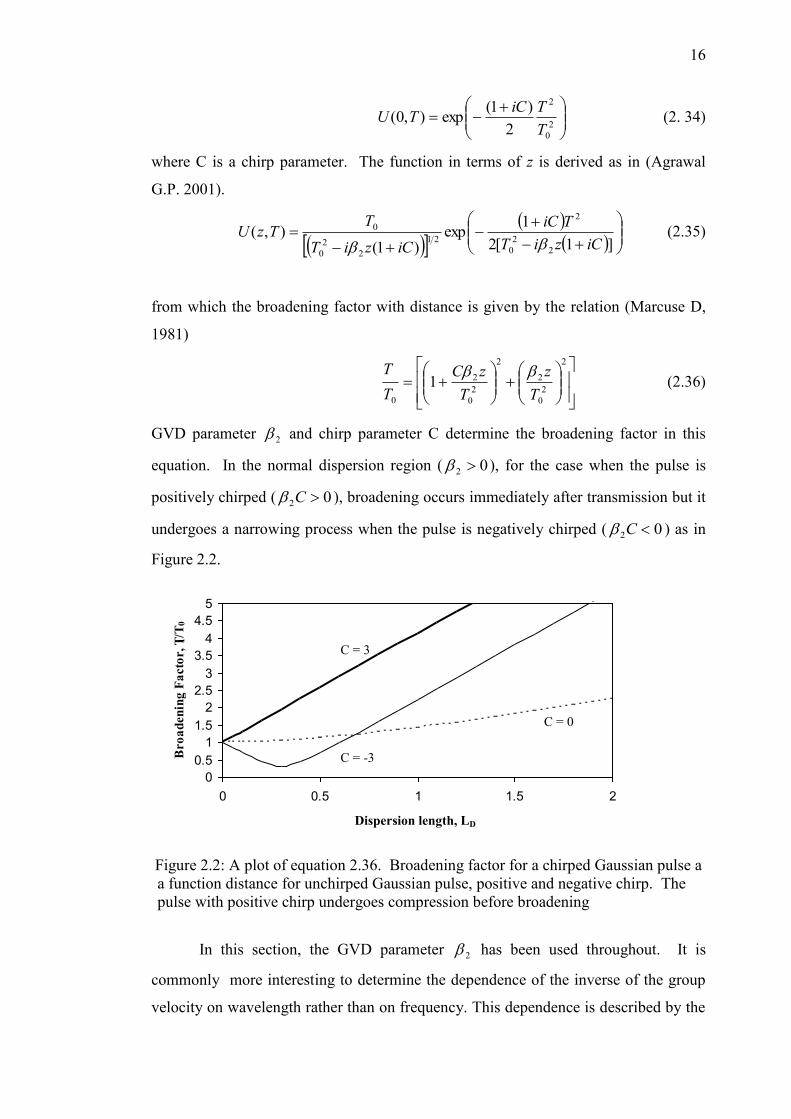
GVD parameter 2 and chirp parameter C determine the broadening factor in this

equation. In the normal dispersion region ( 02 ), for the case when the pulse is

positively chirped ( 02 C ), broadening occurs immediately after transmission but it

undergoes a narrowing process when the pulse is negatively chirped ( 02 C ) as in

Figure 2.2.

0

0.5

1

1.5

2

2.5

3

3.5

4

4.5

5

0 0.5 1 1.5 2

Distance, z

Bro

ad

en

ing

Fa

cto

r, T 1

/T0

Figure 2.2: A plot of equation 2.36. Broadening factor for a chirped Gaussian pulse a

a function distance for unchirped Gaussian pulse, positive and negative chirp. The

pulse with positive chirp undergoes compression before broadening

In this section, the GVD parameter 2 has been used throughout. It is

commonly more interesting to determine the dependence of the inverse of the group

velocity on wavelength rather than on frequency. This dependence is described by the

C = -3

C = 3

C = 0

Dispersion length, LD

17

dispersion parameter D and its slope with respect to wavelength, λ. The following

relationships hold

22

21

c

vd

dD

g

or D

cvd

d

g

2

1 2

2

(2.37)

D is typically measured in units ps/nm-km. It determines the broadening for a pulse of

bandwidth after propagating over a distance z, or equivalently, the time offset of

two pulses after a distance z, which are separated in the spectral domain by . The

relationship between dispersion and wavelength is described in Figure 2.3 and

between normal and anomalous dispersion and wavelength, in Figure 2.4.

Figure 2.3: Variation of the dispersion parameter D with wavelength for a standard

monomode fibre showing that zero dispersion occurs at m 3.1 (Li T., 1985).

Figure 2.4: Anomalous and normal dispersion regimes (Li T., 1985).

18

2.1.2 Pulse propagation governed by SPM

In this section, the effect of dispersion term in equation 2.18 is considered to be

negligible compared to the nonlinear term. In that case the pulse evolution is governed

by nonlinear effect that leads to spectral broadening of the pulse (Agrawal G.P. 2001).

This happens when the fibre length L is such that NLD LLL or equivalently.

12

2

00

TP

L

L

NL

D (2.38)

In standard single mode fibres, this condition holds for relative long pulses

( ps1000 ) and peak power P0 ~ 1W .

To study the effect of SPM mathematically (where the effect of dispersion 02 and

taking into account the effect of loss, α in equation 2.6 and using the same process in

section 2.1.1, we have

UUL

zi

z

U

NL

2)exp(

(2.39)

where accounts for fibre loss, which plays an important part in the pulse

propagation and )1( 0PLNL is the nonlinear length. The nonlinear parameter, is

related to the nonlinear index coefficient n2 by effcAn 02 . Equation 2.39 can be

solved to give the solution

)),(exp(),0(),( TziTUTzU NL (2.40)

where ),0( TU is the input pulse amplitude at z = 0 and NL is the nonlinear phase

shift which increases with fibre length, L given by

NL

eff

NLL

zTUTz

2),0(),( . (2.41)

with the effective transmission distance effz (which is smaller than z due to fibre

losses) given by

)exp(1 zzeff (2.42)

The maximum pulse shift occurs at the centre of the pulse T = 0 with magnitude of

effNLeff zPLz 0max (2.43)

where 1

0 )( PLNL .

19

This shows the physical significance of NLL that is the effective propagation distance

at which 1max .

To impose a frequency chirp on the pulse, take the partial derivative of the phase shift

in equation 2.41 with respect to T,

2

),0( TUTL

z

T NL

effNL

(2.44)

This frequency chirp is now time dependent and increases with magnitude as the

propagation distance increases. New frequencies are self-generated leading to spectral

broadening. To see the SPM effect in spectral broadening consider a super- Gaussian

pulse with an initial field given by

m

TTU

2

02

1exp),0(

(2.45)

The SPM-induced chirp )(T for this pulse is

mm

NL

eff TT

L

z

T

mT

2

0

12

00

exp2

)(

(2.46)

where m is the order of super Gaussian pulse (m=1 is for Gaussian).

From equation 2.45 and 2.46 the relationship between phase and the corresponding

time is plotted using m = 1 and m = 4 and is presented in figures 2.5 and 2.6.

-4 -3 -2 -1 0 1 2 3 40

0.2

0.4

0.6

0.8

1

Time

Phase

m = 4

m = 1

Figure 2.5: A plot of equation 2.46. The effect of transmission of a pulse with a unit

width T0 and effective transmission distance equal to the non linear length LNL.

Amplitude of 1st and 4th order Gaussian pulses with time.

20

-5 -4 -3 -2 -1 0 1 2 3 4 5

-3

-2

-1

0

1

2

3

Time

Chirp

m = 4

m = 1

Figure 2.6: A plot of equation 2.46. The effect of transmission of a pulse with a unit

width T0 and effective transmission distance equal to the non linear length LNL.

Induced chirp caused by phase changes across 1st and 4th order Gaussian pulses.

2.1.3 Pulse Propagation Governed by GVD and SPM

Previously GVD and SPM were treated separately. In this section the case is

considered when the fibre length DLL and NLLL where dispersion and

nonlinearity act together as the pulse propagates along the fibre. Temporal and

spectral changes that occur when the effect of GVD and SPM are combined, are

considered in this section.

To start with, consider the lossless case of equation 2.6. The NLSE equation can then

be written as

AAT

A

z

Ai

2

2

2

22

1

(2.50)

This equation can be normalized using

00 P

ANNUu

P

AU ,

DL

zZ ,

0T

T (2.51)

to give

UUNU

Z

Ui

22

2

2

22

1sgn

(2.52)

21

where N is defined as

2

2

002

TP

L

LN

NL

D . (2.53)

Eliminating N from equation 2.52 by introducing ALNUu D to take the

standard form of NLSE:

02

1 2

2

2

uu

u

Z

ui

(2.54)

where 1)sgn( 2 is taken for anomalous GVD; for normal dispersion regime, the

dispersive term (2nd

term in equation 2.54) should be negative.

The parameter N governs the relative importance of the effects of GVD and SPM on

the pulse propagation:

1N : dispersive effects are dominant

1N : nonlinear effects are dominant

1N : both dispersive and nonlinear effects are important

1N : SPM and GVD are in the anomalous and normal dispersion regimes

Consider again equations 2.33 and 2.46. The evolution of the shape of an initially

unchirped Gaussian pulse in a normal-dispersion regime of a lossless fibre is shown in

figure 2.7. The pulse broadens more rapidly with the presence of SPM (N=1). This

can be understood by recalling that new frequency components that are red-shifted

near the leading edge and blue-shifted near the trailing edge of the pulse, are generated

continuously as it propagates down the fibre. “In the normal-dispersion regime, the

red components are traveling faster than the blue components, SPM leads to an

enhanced rate of pulse broadening compared with the expected from GVD alone”

(Agrawal G.P, 2001). But the situation is different when considering pulses

propagating in the anomalous-dispersion regime as in figure 2.8. This is due to a

negative sign of 2 in equation 2.33. “The pulse broadens initially at a rate much

lower than that expected in the absence of SPM and then appears to reach a steady

state for DLz 4 ” (Agrawal G.P 2001).

22

Figure 2.7: Evolution of pulse shapes over a distance z/LD for an initially unchirped

Gaussian pulse propagating in the normal dispersion regime of the

fibre (Agrawal G.P,2001).

Figure 2.8: Evolution of pulse shapes over a distance z/LD for an initially unchirped

Gaussian pulse propagating in the anomalous dispersion regime of the

fibre. (Agrawal G.P, 2001)

2.2 Optical solitons: characteristics and conditions for propagation

The existence of solitons in optical fibre is a result of interplay between the dispersive

(GVD) and nonlinearity (SPM) effects. Optical solitons are pulses that exhibit

particular shape and intensity, so there is a perfect balance between the frequency

chirps produced by the GVD in the anomalous dispersion regime and the SPM. This

section discusses the properties of solitons in lossless media. The fundamental soliton

23

has a shape which remains unchanged during propagation while higher order solitons

have a shape which evolves periodically. This section also looks at the interaction

between solitons, where two solitons that collide in a fibre recover their shape and

initial intensity after the collision.

2.2.1 Fundamental and higher order solitons

The mathematical description of solitons employs the NLSE. Consider again equation

2.54. The solution to this equation was first solved using the inverse scattering

method (Zakharov V.E. & Shabat A.B. 1972, Miwa T, 1999). Consider the first order

(N=1) solution of NLSE which has the general form of solution

)2exp()2( sec2),( 2 zihzu (2.55)

where is the soliton amplitude. Normalising )0,0(u by setting 12 gives the

fundamental (N=1) soliton solution in the form of hyperbolic-secant,

)2/exp()(sec),( izhzu (2.56)

This equation indicates that if the hyperbolic-secant pulse whose width 0T and the

peak power 0P are chosen such that 1N in equation 2.53 then

2

0

2

0T

P

(2.57)

is launched into an ideal lossless optical fibre, thus it will propagate undistorted

indefinitely with no change in shape. Equation 2.57 shows that the peak power is

inversely proportional to the square of the pulsewidth. The further solution to the

NLSE is

)(sec),0( hNu (2.58)

where N is an integer related to the soliton order. From equation 2.53, the required

peak power is 2N times that of a fundamental soliton for the same pulsewidth.

Higher order solitons, corresponding to 1N , do not maintain their shape during

propagation along the fibre. This is due to the unusual evolution process where pulse

splitting occurs during transmission only for the pulses to reform back into its original

form at 2/mz , where m is an integer. Thus the distance or the soliton period at

which a higher order soliton recovers its original shape is given by

24

2

2

0

022

TLz D (2.59)

To understand the reason for the stable solution it is useful to consider the sign

of the chirps induced on the pulse by GVD and SPM. The sign of the GVD induced

chirp depends on the sign of the 2 (positive or negative sign in normal- or

anomalous-dispersion regime respectively) whilst that of the SPM induced chirp is

always of the same sign since the frequency shift is opposite to the gradient of the

pulse power profile. In the anomalous-dispersion regime, the two chirps are opposed

and can cancel out to form a stable soliton whilst in the normal-dispersion regime they

have the same sign and do not cancel out, thus accumulate with transmission to

produce unstable pulses.

2.2.2 Interaction between solitons

In order to increase the information carried in the transmission system, it is desirable

to launch the pulses close together. Unfortunately the overlap of the closely spaced

solitons leads to mutual interaction and therefore to serious performance degradation

of the soliton transmission system. This is as a result of the small finite tails of the

soliton that extend into neighboring solitons which in turn form a superposition that

causes them to propagate at different velocities (Gordon G.P 1983). Another study

showed that the inclusion of fibre loss also leads to dramatic increase in soliton

interactions (Blow K.J, Doran N.J 1983). Several schemes for the reduction of the

pulse interaction have been proposed; the use of Gaussian-shaped pulses (Chu P.L,

Desem C. 1983), introduction of phase difference between neighboring solitons

(Anderson D., Lisak M. 1986), the use of third order dispersion (Chu P.L, Desem C.

1985, 1987) are among others.

Consider a pair of solitons at the input of transmission line which can be

described by

iqrrhrqhu exp)(secsec),0( 00 (2.60)

Where 02q is the initial (normalised) separation ( 002 TTq B and B is the bit rate), r

is the relative amplitude and is the relative phase of the two input pulses. The

interaction of the pulses depends on their relative amplitude, r and relative phase, .

Numerical simulations and calculations have shown that for equal phase( 0 ) and

147

REFERENCES

Agrawal, G.P (2001). Nonlinear fiber optics. 3rd. ed. London: Academic Press.

Agrawal G.P (2002)., Fiber-Optic Communication Systems. 3rd. ed. New York: John

Wiley and sons.

Alexander S.B. (1997). Optical Communication Receiver Design.: SPIE Optical

Engineering Press, Washington USA, Institution of Electrical Engineers,

London, UK

Anderson D, Lisak M (1986). Bandwidth limits due to mutual pulse interaction in

optical soliton communication systems. Opt. Lett,. 11(3).pp 174-176

Becker P.C., Olsson N.A., Simpson J.R (1999). Erbium-doped fiber amplifiers,

fundamentals and technology. San Diego: Academic Press.

Bergano N. S., Kerfoot F. W., Davidson C. R. (1993). Margin Measurements in

optical amplifier system, Photonics Technology Letter, 5, pp. 304-306

Blow K.J, Doran N.J (1983)., Bandwidth limits of nonlinear (soliton) optical

communication systems. Elec. Lett., 19(11): pp. 429-430.

Blow K.J, Doran N.J (1991). Average soliton Dynamics and the operation of soliton

systems with lumped amplifiers. IEEE photonics Technology Letters. 3(4): pp.

369-371.

Chu P.L, Desem C (1983). Gaussian pulse propagation in nonlinear optical fibre.

Elec. Lett., 19(23): pp. 956-957.

Chu P.L, Desem C (1985). Effect of third-order dispersion of optical fibre on soliton

interaction. Elec. Lett., 21(6): pp. 228-229.

Chu P.L, Desem .C (1987). Soliton interaction in the presence of loss and periodic

amplification in optical fibers. Opt. Lett., 12(5): pp. 349-351.

Desurvive E(2001)., Erbium-doped fiber amplifiers,principles and applications. New

York: John-Wiley and sons.

Desurvire E., Simpson J.R and Becker P.C (1987). High gain erbium-doped traveling-

wave amplifier. Opt. Lett., 12(11): p. 888-890.

Eberhard, M.A (2004). mqocss, version 2.0.4, released 21 Sept 2004: unpublished.

Eberhard M. A, Blow K.J(2005). Numerical Q parameter estimates for scalar and

vector models in optical communication system simulations. Optics

Communications. 249(4-6): pp. 421-429.

148

Eberhard M. A, Blow K.J (2006). Q parameter estimation using numerical simulations

for linear and nonlinear transmission systems. Optics Communications.

265(1): pp. 73-78.

Evans A.F, Wright J.V (1995). Constraints on the design of single-channel, high-

capacity soliton systems. IEEE photonics Technology Letters. 7(1): p. 117-

119.

Ferreira, M.F.S. (1999). Design constraints of high-bit-rate soliton communication

system. in CLEO. Pacific Rim.

Gordon J. P., (1992). Dispersive perturbations of solitons of the nonlinear Schrödinger

equation. J. Opt. Soc. Am. B9: pp91-97

Gordon, J.P., Mollenauer, L.F (1991). Effects of fiber nonlinearities and amplifier

spacing on ultra-long distance transmission. J.Lightwave Technology. LT-9:

pp. 171-173.

Gordon J.P, Haus A.H (1986). Random walk of coherently amplified solitons in

optical fiber transmission. Optics Letters, 11(10): pp. 665-667.

Gordon J.P (1983). Interaction forces among solitons in optical fibers. Opt. Lett.,

8(11): pp. 596.

Hanna M, Porte H (1999). et. al., Soliton optical phase control by use of in-line filters.

Opt. Lett,. 24(11): pp. 732-734.

Hasegawa A and Tappert F,(1973). Transmission of stationary nonlinear optical

pulses in dispersive dielectric fibers. I. Anomalous dispersion. Appl. Phys.

Lett. 23, 142–144.

Hasegawa A and Tappert F,(1973). Transmission of stationary nonlinear optical

pulses in dispersive dielectric fibers. II. Normal dispersion. Appl. Phys. Lett.

23, 171–172.

Hasegawa A., Kodama Y (1990). Guiding Centre Soliton in Optical Fibre. Opt. Lett.,.

15(24): pp. 1443-1445.

Hasegawa A., Kodama Y (1991). Guiding-center soliton in fibers with periodically

varying dispersion. Opt. Lett,. 16(18): pp. 1385-1387.

Hasegawa A (1984), Numerical study of optical soliton transmission amplified

periodically by the stimulated Raman process. Appl. Opt.23: pp. 3302.

Hasegawa A (1983), Amplification and reshaping of optical solitons in a glass fiber -

IV: Use of stimulated Raman process. Opt. Lett,. 8: pp. 650.

Harboe P. B., Souza J.R.(2002), Soliton control with fixed and sliding-frequency

filters revisited. Journal of Microwaves and Optoelectronics. 2(6): p. 11-20.

149

Horiguchi M., Osanai H (1976). Spectral losses of low-OH-content optical fibers.

Elec. Lett. 12: pp. 310-312.

Iannone E., Matera F., Mecozzi A., and Settembre M (1998). Nonlinear Optical

Communication Networks: Wiley, New York.

Kodama Y, Hasegawa A (1983), Amplification and reshaping of optical solitons in

glass fiber - III. amplifiers with random gain. Opt. Lett. 8. p. 342.

Kaiser G. (2000), Optical fiber communications. 3rd ed. Boston: McGraw-Hill.

Kodama Y, Hasegawa A (1992). Generation of asymtotically stable optical solitons

and suppression of the Gordon-Haus effect. Optics Letters, 17(1): pp. 31-33.

Kivshar, Y.S (2003), Optical solitons: from fibers to photonic crystals. London: Acad.

Press.

Kaminov I.P, Lee T, Willner A. E. (2008). Optical Fiber Telecommunications V B.

USA: Elsevier.

Marcuse, D (1991). Theory of dielectric optical waveguides. 2nd ed. London:

Academic Press. pp. 336-341.

Marcuse, D (1980). Pulse distortion in single-mode fibers. Appl. Opt.,. 19(10): pp.

1653.

Marcuse, D (1981). Pulse distortion in single-mode fiber part 2. Appl. Opt., 20(17):

pp. 2969-2974.

Marcuse D (1992). Simulations to demonstrate reduction of the Gordon-Haus effect.

Optics Letters. 17(1): pp. 34-36.

Matera F, Settembre M (1996). Comparison of the performance of optically amplified

transmission systems. J. Lightwave Technology. 14(1): pp. 1-12.

Matera F, Settembre M (1994), Nonlinear compensation of chromatic dispersion for

phase- and intensity-modulated signals in the presence of amplified

spontaneous emission noise. Opt. Lett,. 19: pp. 1198-1200.

Mears R.J., Reekie L., Jauncey I.M. and Payne D.N.(1987), Low noise erbium doped

fiber amplifier operating at 1.54 micron. Elec. Lett., 23: pp. 1026-1028.

Mecozzi, A., Moores J.D, Haus,H.A (1992). Modulation and filtering control of

soliton transmission. J. Opt. Soc. Am. 9: pp. 1350-1357.

Mecozzi A, Moores J.D, Haus H.A.Lai Y (1991). Soliton transmission control. Opt.

Lett,. 16(23): pp. 1841-43.

Michael, M (2000). XML, Programming Languages, Data Processing. Indianapolis:

Sams Publishing.

150

Midrio M, Romagnoli M, Wabnitz S, Franco P (1996). Relaxation of guiding center

solitons in optical fibers. Opt. Lett,. 21(17): pp. 1351-1353.

Miller S.E., Kaminov I.P, (1988) 1st ed. Optical Fiber Telecommunications II, 2

nd edn.

Orlando: Academic Press, Inc. 995.

Miwa T (1999). Mathematics of solitons. New York: Cambridge University Press.

Mitschke F.M, Mollenauer L.F (1987). Experimental observation of interaction forces

between solitons in optical fibers. Opt. Lett, 1987. 12(5): pp. 355-357.

Mollenauer L. F. et al.( 1993), Demonstration using sliding-frequency guiding filters,

of error-free soliton transmission over 20Mm at 10 Gbits/s, single channel and

over more than 13 Mm at 20 Gbits/s in a two-channel WDM. Electron Letter,

29: pp910-911

Mollenauer L.F, Gordon J.P.( 1986)., Islam M.N, Soliton propagation in long fibers

with periodically compensated loss. IEEE J. Quantum Electron,. QE-22: pp.

157.

Mollenauer L.F., Smith K (1988)., Demonstration of soliton transmission over more

than 4000 km in fibre with loss periodically compensated by Raman gain. Opt.

Lett,. 13(8): pp. 675-677.

Mollenauer L.F., Evangelides S.G, Haus H.A (1991)., Long-Distance Soliton

Propagation using Lumped Amplifiers and Dispersion Shifted Fiber. Journal

of Lightwave Technology, 9(2): pp. 194-197.

Mollenauer L.F., Stolen R.H, Islam M.N(1985). Experimental demonstration of

soliton propagation in long fibers: loss compensated by Raman gain. Opt.

Lett,. 10(5). pp. 229-231.

Shiojiri E, Fujii Y (1985). Transmission capability of an optical fiber communication

system using index nonlinearity. Appl. Opt., 24: pp. 358.

Senior, J.M (1992). Optical Communication Theory, Communications Engineering.

2nd ed. New York, London: Prentice Hall.

T. Li (1985). Optical Fiber Communications: Fiber Fabrication. vol. 1. San Diego:

Academic Press

Taylor J.R (2005)., Optical Solitons Theory and Experiment. New York: Cambridge

University Press.

Wrights J. V, Carter S.F (1991). Constraints on the design of long-haul soliton

systems. in Proc. Tech. Digest, Conf. Nonlinear Guided-Wave Phenomena.

vol. 1, pp. 89-92.

151

Yamada J.I, Machida S.., Kimura T (1981)., Ultimate low-loss single mode fiber.

Elec. Lett., 15: pp. 106-108.

Zakharov V.E., Shabat A.B (1972). Exact theory of two-dimensional self-focusing and

one-dimension self modulation of waves in nonlinear media. Sov. Physics,

JETP 34: pp. 62.

http://www.corningfiber.com,http://www.lucent,http://www.furukawa.jp.

Online Documentation/Manuals for VPI-Photonics Module Reference Manual

Online Documentation/Manuals for OptSim- Photonics Module Reference Manual

152

PROCEEDINGS

K.J. Blow, S Turitsyn, S Derevyanko, J Prilepsky,Z Zakaria (2009) Soliton in optical

communication. Int. conference on Engineering and Computational Maths,

Hong Kong Polytech Uni.

Zakaria Z, Eberhard M. A, Blow K. J. (2009). An amplified single channel soliton

pulse propagation in optical fibres at 3500 km distance. Proceeding The First

Seminar on Science and Technology (ISSTEC).UII Jogjakarta. pp 65-70

Zahariah Z. (2011). Analytical model and limitations on the design diagram for soliton

systems. 2nd

ICP2011. Kota Kinabalu. pp 151-155

Zahariah Z. (2011). Performance comparison between analytical analysis and

numerical simulations for average soliton system. ISASM 2011. Kuala

Lumpur.