Reinforcement Learning Generalization and Function Approximation

Novel Function Approximation Techniques for
Large-scale Reinforcement Learning
A Dissertation
by
Cheng Wu
to
the Graduate School of Engineering
in Partial Fulfillment of the Requirements
for the Degree of
Doctor of Philosophy
in the field of
Computer Engineering
Advisor: Prof. Waleed Meleis
Northeastern University
Boston, Massachusetts
April 2010 in which submitted to GPO

c© Copyright May 2010 conferred by Cheng Wu
All Rights Reserved
ii

NORTHEASTERN UNIVERSITY
Graduate School of Engineering
Thesis Title: Novel Function Approximation Techniques for Large-scale Reinforcement
Learning.
Author: Cheng Wu.
Program: Computer Engineering
Approved for Dissertation Requirements of the Doctor of Philosophy Degree:
Thesis Advisor: Waleed Meleis Date
Thesis Reader: Jennifer Dy Date
Thesis Reader: Javed A. Aslam Date
Chairman of Department: Date
Graduate School Notified of Acceptance:
Director of the Graduate School: Date
iii

Contents
1 Introduction 1
1.1 Reinforcement Learning . . . . . . . . . . . . . . . . . . . . . . . . . . . . . 3
1.2 Function Approximation . . . . . . . . . . . . . . . . . . . . . . . . . . . . . 5
1.2.1 Function Approximation Using Natural Features . . . . . . . . . . . . 8
1.2.2 Function Approximation Using Basis Functions . . . . . . . . . . . . 10
1.2.3 Function Approximation Using SDM . . . . . . . . . . . . . . . . . . 12
1.3 Our Application Domain . . . . . . . . . . . . . . . . . . . . . . . . . . . . . 13
1.4 Dissertation Outline . . . . . . . . . . . . . . . . . . . . . . . . . . . . . . . 15
2 Adaptive Function Approximation 19
2.1 Experimental Evaluation: Traditional Function Approximation . . . . . . . . 20
2.1.1 Application Instances . . . . . . . . . . . . . . . . . . . . . . . . . . . 20
2.1.2 Performance Evaluation of Traditional Tile Coding . . . . . . . . . . 22
2.1.3 Performance Evaluation of Traditional Kanerva Coding . . . . . . . . 25
2.2 Visit Frequency and Feature Distribution . . . . . . . . . . . . . . . . . . . . 28
iv

2.3 Adaptive Mechanism in Kanerva-Based Function Approximation . . . . . . . 31
2.3.1 Prototype Deletion and Generation . . . . . . . . . . . . . . . . . . . 32
2.3.2 Performance Evaluation of Adaptive Kanerva-Based Function Approx-
imation . . . . . . . . . . . . . . . . . . . . . . . . . . . . . . . . . . 34
2.4 Summary . . . . . . . . . . . . . . . . . . . . . . . . . . . . . . . . . . . . . 37
3 Fuzzy Logic-based Function Approximation 38
3.1 Experimental Evaluation: Kanerva Coding Applied to Hard Instances . . . . 39
3.2 Prototype Collisions in Kanerva Coding . . . . . . . . . . . . . . . . . . . . 41
3.3 Adaptive Fuzzy Kanerva Coding . . . . . . . . . . . . . . . . . . . . . . . . . 48
3.3.1 Fuzzy and Adaptive Mechanism . . . . . . . . . . . . . . . . . . . . . 49
3.3.2 Adaptive Fuzzy Kanerva Coding Algorithm . . . . . . . . . . . . . . 51
3.3.3 Performance Evaluation of Adaptive Fuzzy Kanerva-Based Function
Approximation . . . . . . . . . . . . . . . . . . . . . . . . . . . . . . 53
3.4 Prototype Tuning . . . . . . . . . . . . . . . . . . . . . . . . . . . . . . . . . 55
3.4.1 Experimental Evaluation: Similarity Analysis of Membership Vectors 55
3.4.2 Tuning Mechanism . . . . . . . . . . . . . . . . . . . . . . . . . . . . 58
3.4.3 Performance Evaluation of Tuning Mechanism . . . . . . . . . . . . . 58
3.5 Summary . . . . . . . . . . . . . . . . . . . . . . . . . . . . . . . . . . . . . 61
4 Rough Sets-based Function Approximation 63
4.1 Experimental Evaluation: Effect of Varying Number of Prototypes . . . . . . 64
v

4.2 Rough Sets and Kanerva Coding . . . . . . . . . . . . . . . . . . . . . . . . 66
4.3 Rough Sets-based Kanerva Coding . . . . . . . . . . . . . . . . . . . . . . . 71
4.3.1 Prototype Deletion and Generation . . . . . . . . . . . . . . . . . . . 73
4.3.2 Rough Sets-based Kanerva Coding Algorithm . . . . . . . . . . . . . 74
4.3.3 Performance Evaluation of Rough Sets-based Kanerva Coding . . . . 77
4.4 Effect of Varying the Number of Initial Prototypes . . . . . . . . . . . . . . 81
4.5 Summary . . . . . . . . . . . . . . . . . . . . . . . . . . . . . . . . . . . . . 83
5 Real-world Application: Cognitive Radio Network 84
5.1 Introduction . . . . . . . . . . . . . . . . . . . . . . . . . . . . . . . . . . . . 84
5.2 Reinforcement Learning-Based Cognitive Radio . . . . . . . . . . . . . . . . 88
5.2.1 Problem Formulation . . . . . . . . . . . . . . . . . . . . . . . . . . . 88
5.2.2 Application to cognitive radio . . . . . . . . . . . . . . . . . . . . . . 89
5.3 Experimental Simulation . . . . . . . . . . . . . . . . . . . . . . . . . . . . . 94
5.3.1 Simulation Setup . . . . . . . . . . . . . . . . . . . . . . . . . . . . . 94
5.3.2 Simulation Evaluation . . . . . . . . . . . . . . . . . . . . . . . . . . 97
5.4 Function Approximation for RL-based Cognitive Radio . . . . . . . . . . . . 102
5.5 Summary . . . . . . . . . . . . . . . . . . . . . . . . . . . . . . . . . . . . . 104
6 Conclusion 106
Bibliography 111
vi

List of Figures
2.1 The grid world of size 32 x 32. . . . . . . . . . . . . . . . . . . . . . . . . . . 21
2.2 The implementation of the tiling. . . . . . . . . . . . . . . . . . . . . . . . . 23
2.3 The fraction of test instances solved by Q-Learning with traditional Tile Cod-
ing with 2000 tiles. . . . . . . . . . . . . . . . . . . . . . . . . . . . . . . . . 24
2.4 The implementation of Kanerva Coding. . . . . . . . . . . . . . . . . . . . . 25
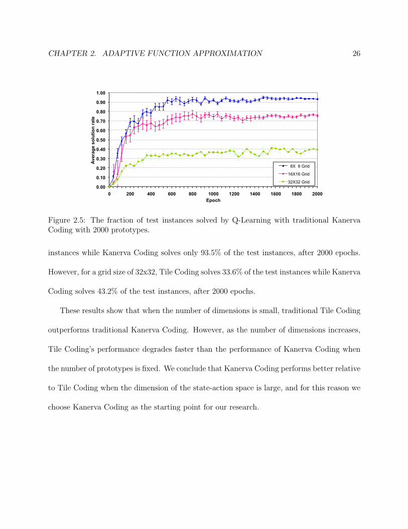
2.5 The fraction of test instances solved by Q-Learning with traditional Kanerva
Coding with 2000 prototypes. . . . . . . . . . . . . . . . . . . . . . . . . . . 27
2.6 The frequency distribution of visits to tiles over a sample run using Q-learning
with Tile Coding . . . . . . . . . . . . . . . . . . . . . . . . . . . . . . . . . 30
2.7 The frequency distribution of visits to prototypes over a sample run using
Q-learning with Kanerva Coding . . . . . . . . . . . . . . . . . . . . . . . . . 30
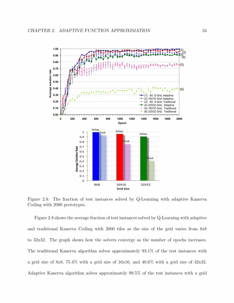
2.8 The fraction of test instances solved by Q-Learning with adaptive Kanerva
Coding with 2000 prototypes. . . . . . . . . . . . . . . . . . . . . . . . . . . 35
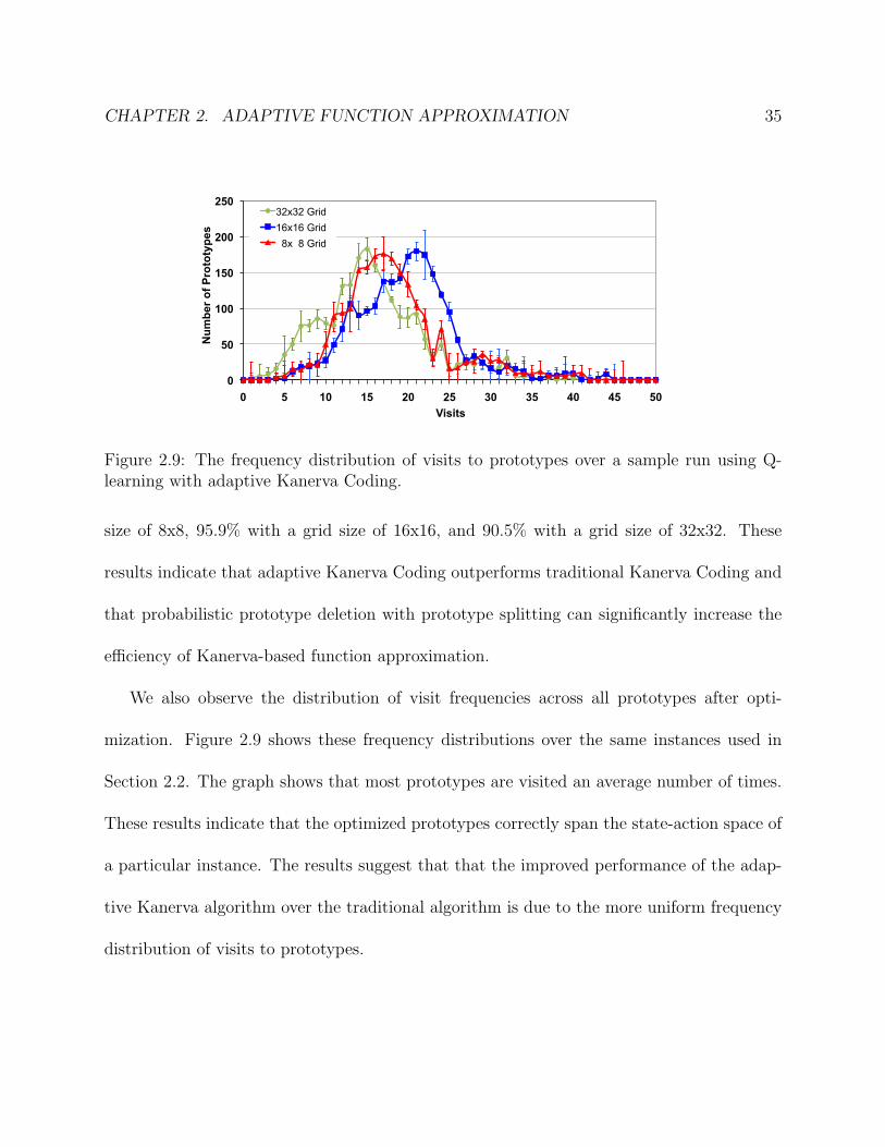
2.9 The frequency distribution of visits to prototypes over a sample run using
Q-learning with adaptive Kanerva Coding. . . . . . . . . . . . . . . . . . . . 36
vii

3.1 The fraction of easy and hard test instances solved by Q-learning with adaptive
Kanerva Coding with 2000 prototypes. . . . . . . . . . . . . . . . . . . . . . 41
3.2 The illustration of prototype collision. (a) adjacent to no prototype; (b) ad-
jacent to an identical prototype set; (c) adjacent to unique prototype vectors. 42
3.3 Prototype collisions using traditional and adaptive Kanerva-based function
approximation with 2000 prototypes. . . . . . . . . . . . . . . . . . . . . . . 44
3.4 Average fraction of test instances solved (solution rate) (a) 8x8 grid; (c) 16x16
grid; (e) 32x32 grid, and the fraction of of state-action pairs that are adjacent
to no prototypes and adjacent to identical prototype vectors (collision rate) (b)
8x8 grid; (d) 16x16 grid; (f) 32x32 grid by traditional and adaptive Kanerva-
based function approximation as the number of prototypes varies from 300 to
2500. . . . . . . . . . . . . . . . . . . . . . . . . . . . . . . . . . . . . . . . . 46
3.5 Sample membership function for traditional Kanerva Coding. . . . . . . . . . 49
3.6 Sample membership function for fuzzy Kanerva Coding. . . . . . . . . . . . . 50
3.7 Average solution rate for adaptive fuzzy Kanerva Coding with 2000 prototypes. 54
3.8 (a) Distribution of membership grades and (b) prototype similarity across
sorted prototypes. . . . . . . . . . . . . . . . . . . . . . . . . . . . . . . . . . 56
3.9 Illustration of the similarity of membership vectors across sparse and dense
prototype regions. . . . . . . . . . . . . . . . . . . . . . . . . . . . . . . . . . 57
3.10 Average solution rate for adaptive fuzzy Kanerva Coding with Tuning using
2000 prototypes. . . . . . . . . . . . . . . . . . . . . . . . . . . . . . . . . . 59
viii

3.11 The four-room gridworld . . . . . . . . . . . . . . . . . . . . . . . . . . . . . 60
3.12 Average solution rate for adaptive Fuzzy Kanerva Coding with Tuning in the
four-room gridworld of size 32x32. . . . . . . . . . . . . . . . . . . . . . . . . 61
4.1 The fraction of hard test instances solved by Q-learning with adaptive Kanerva
Coding as the number of prototypes decreases. . . . . . . . . . . . . . . . . . 66
4.2 Illustration of equivalence classes of the sample. . . . . . . . . . . . . . . . . 68
4.3 The fraction of equivalence classes that contain two or more state-action pairs
over all equivalence classes, the conflict rate, and its corresponding solution
rate and collision rate using traditional Kanerva and adaptive Kanerva with
frequency-based prototype optimization across all sizes of grids . . . . . . . . 70
4.4 The fraction of prototypes remaining after performing a prototype reduct
using traditional and optimized Kanerva-based function approximation with
2000 prototypes. The original and final number of prototypes is shown on
each bar. . . . . . . . . . . . . . . . . . . . . . . . . . . . . . . . . . . . . . . 72
4.5 Average solution rate for traditional Kanerva, adaptive Kanerva and rough
sets-based Kanerva (a), in 8x8 grid; (b), in 16x16 grid; (c), in 32x32 grid. . . 78
4.6 Effect of rough sets-based Kanerva on the number of prototypes and the frac-
tion of equivalence classes (a), in 8x8 grid; (b), in 16x16 grid; (c), in 32x32
grid. . . . . . . . . . . . . . . . . . . . . . . . . . . . . . . . . . . . . . . . . 80
4.7 Variation in the number of prototypes with different numbers of initial proto-
types with rough sets-based Kanerva in a 16x16 grid. . . . . . . . . . . . . . 82
ix

5.1 The CR ad hoc architecture . . . . . . . . . . . . . . . . . . . . . . . . . . . 86
5.2 The cognitive radio cycle for the CR ad hoc architecture . . . . . . . . . . . 87
5.3 Multi-agent reinforcement learning based cognitive radio. . . . . . . . . . . . 90
5.4 Comparative reward levels for different observed scenarios . . . . . . . . . . 92
5.5 Block diagram of the implemented simulator tool for reinforcement learning
based cognitive radio. . . . . . . . . . . . . . . . . . . . . . . . . . . . . . . . 94
5.6 The performance of small topology. . . . . . . . . . . . . . . . . . . . . . . . 98
5.7 The performance of the real-world topology with five different node densities. 100
5.8 Average probability of successful transmission for the real-world topology with
500 nodes. . . . . . . . . . . . . . . . . . . . . . . . . . . . . . . . . . . . . . 103
x

List of Tables
2.1 The average fraction of test instances solved by Q-learning with traditional
Tile Coding. . . . . . . . . . . . . . . . . . . . . . . . . . . . . . . . . . . . . 24
2.2 The average fraction of test instances solved by Q-learning with traditional
Kanerva Coding. . . . . . . . . . . . . . . . . . . . . . . . . . . . . . . . . . 26
2.3 The average fraction of test instances solved by Q-learning with adaptive
Kanerva Coding. . . . . . . . . . . . . . . . . . . . . . . . . . . . . . . . . . 34
3.1 The average fraction of test instances solved by Q-learning with adaptive
Kanerva Coding. . . . . . . . . . . . . . . . . . . . . . . . . . . . . . . . . . 40
3.2 The average fraction of test instances solved by Q-Learning with adaptive
fuzzy Kanerva Coding. . . . . . . . . . . . . . . . . . . . . . . . . . . . . . . 53
4.1 The average fraction of test instances solved by Q-Learning with adaptive
Kanerva Coding. . . . . . . . . . . . . . . . . . . . . . . . . . . . . . . . . . 65
4.2 Sample of adjacency between state-action pairs and prototypes. . . . . . . . 67
xi

4.3 Percentage improved performance of rough sets-based Kanerva over adaptive
Kanerva. . . . . . . . . . . . . . . . . . . . . . . . . . . . . . . . . . . . . . . 79
xii

Abstract
Function approximation can be used to improve the performance of reinforcement learn-
ers. Traditional techniques, including Tile Coding and Kanerva Coding, can give poor
performance when applied to large-scale problems. In our preliminary work, we show that
this poor performance is caused by prototype collisions and uneven prototype visit frequency
distributions. We describe our adaptive Kanerva-based function approximation algorithm,
based on dynamic prototype allocation and adaptation. We show that probabilistic proto-
type deletion with prototype splitting can make the distribution of visit frequencies more
uniform, and that dynamic prototype allocation and adaptation can reduce prototoype coll-
sisions. This approach can significantly improve the performance of a reinforcement learner.
We then show that fuzzy Kanerva-based function approximation can reduce the similarity
between the membership vectors of state-action pairs, giving even better results. We use
Maximum Likelihood Estimation to adjust the variances of basis functions and tune the
receptive fields of prototypes. This approach completely eliminates prototype collisions, and
greatly improve the ability of a Kanerva-based reinforcement learner to solve large-scale
problems.
Since the number of prototypes remains hard to select, we describe a more effective
approach for adaptively selecting the number of prototypes. Our new rough sets-based
Kanerva-based function approximation uses rough sets theory to explain how prototype

2
collisions occur. Our algorithm eliminates unnecessary prototypes by replacing the original
prototype set with its reduct, and reduces prototype collisions by splitting equivalence classes
with two or more state-action pairs. The approach can adaptively select an effective number
of prototypes and greatly improve a Kanerva-based reinforcement learners ability.
Finally, we apply function approximation techniques to scale up the ability of reinforce-
ment learners to solve a real-world application: spectrum management in cognitive radio
networks. We use multi-agent reinforcement learning approach with decentralized control
can be used to select transmission parameters and enable efficient assignment of spectrum
and transmit powers. However, the requirement of RL-based approaches that an estimated
value be stored for every state greatly limits the size and complexity of CR networks that
can be solved. We show that function approximation can reduce the memory used for large
networks with little loss of performance. We conclude that our spectrum management ap-
proach based on reinforcement learning with Kanerva-based function approximation can
significantly reduce interference to licensed users, while maintaining a high probability of
successful transmissions in a cognitive radio ad hoc network.

Chapter 1
Introduction
Machine learning, a field of artificial intelligence, can be used to solve search problems using
prior knowledge, known experience and data. Many powerful computational and statistical
paradigms have been developed, including supervised learning, unsupervised learning, trial-
and-error learning and reinforcement learning.
However, machine learning techniques can struggle to solve large-scale problems with huge
state and action spaces [12]. Various solutions to this problem under have been studied, such
as dimensionality reduction [2], principle component analysis [22], support vector machines
[14], and function approximation [17].
Reinforcement learning, one of the most successful machine learning paradigms, enables
learning from feedback received through interactions with an external environment. Like the
other paradigms for machine learning, a key drawback of reinforcement learning is that it
only works well for small problems, and performs poorly for large-scale problems [43].
1

CHAPTER 1. INTRODUCTION 2
Function approximation [17, 40] is a technique for resolving this problem within the
context of reinforcement learning. Instead of using a look-up table to directly store values
of points within the state and action space, it uses examples of the desired value function to
reconstruct an approximation of this function and compute an estimate of the desired value
from the approximation function.
When using many function approximation techniques, a complex parametric approxima-
tion architecture is used to compute good estimates of the desired value function [34]. An
approximation architecture is a computational structure that uses parametric functions to
approximate the value of a state or state-action pair. Using a simple approximation ar-
chitecture design often make estimates diverge from the desired value function, and makes
agents perform inefficiently [10]. Unfortunately, a complex parametric architecture may also
greatly increase the computational complexity of the function approximator itself [11].
Furthermore, large-scale problems can remain hard to solve in practice, even when the
complex architecture is applied. The key to a successful function approximator is not only
the choice of the parametric approximation architecture, but also the choices of various
control parameters under this architecture. Until recently, these choices were typically made
manually, based only on the designer’s intuition [11, 27].
In this dissertation we address the issue of solving large-scale, high-dimension prob-
lems using reinforcement learning with function approximation. We propose to develop a
novel parametric approximation architecture and corresponding parameter-tuning methods
for achieving better learning performance. This framework should satisfy several criteria: (1)

CHAPTER 1. INTRODUCTION 3
it should give accurate approximation, (2) the approximation should be local, that is, appro-
priate for a specific learning problem, (3) the parameters should be selected automatically,
and (4) it should learn online.
We first review related work on reinforcement learning and function approximation, de-
scribe their characteristics and limitations, and give examples of their operation.
1.1 Reinforcement Learning
Reinforcement learning is inspired by psychological learning theory from biology [46]. The
general idea is that within an environment, a learning agent attempts to perform optimal
actions to maximize long-term rewards achieved by interacting with the environment. An
environment is a model of a specific problem domain, typically formulated as a Markov
Decision Process (MDP) [32]. A state is some information that an agent can perceive within
the environment. An action is the behavior of an agent at a specific time at a specific state.
A reward is a measure of the desirability of an agent’s action at a specific state within the
environment.
The classic reinforcement learning algorithm is formulated as follows. At each time
t, the agent perceives its current state st ∈ S and the set of possible actions Ast . The
agent chooses an action a ∈ Ast and receives from the environment a new state st+1 and
a reward rt+1. Based on these interactions, the reinforcement learning agent must develop
a policy π : S → A which maximizes the long-term reward R =∑
t γrt for MDPs, where
0 ≤ γ ≤ 1 is a discounting factor for subsequent rewards. The long-term reward is the

CHAPTER 1. INTRODUCTION 4
expected accumulated reward for the policy.
This implementation of reinforcement learning embodies three important characteris-
tics: a human-like learning framework, the concept of a value function, and online learning.
These three characteristics distinguish reinforcement learning from other machine learning
paradigms, but they can also limit its effectiveness.
The human-like framework defines the interaction between agents and the external en-
vironment in terms of states, actions and rewards, which allows reinforcement learning to
solve the types of problems solved by humans. These types of problems tend to involve a
very large number of states and actions. Unfortunately, the performance of reinforcement
learning is very sensitive to the number of states and actions.
A value function is a function which specifies the accumulated rewards that an agent
expects to receive in the future. While a reward determines the immediate and short-term
value of an action in the current state, a value function gives the expected accumulated and
long-term value of an action under subsequent states.
The concept of a value function distinguishes reinforcement learning from evolutionary
methods [9, 7, 15]. Instead of directly searching the entire policy space by evolutionary
evaluation, a value function evaluates an action’s desirability at the current state by accu-
mulating delayed rewards. In reinforcement learning, the accuracy and efficiency of a value
function is closely related to the performance of a reinforcement learner.
In an online learning system, learning and the evaluation of the learning system occur
concurrently. However, in order to maintain this concurrency, a reinforcement learner must

CHAPTER 1. INTRODUCTION 5
compute the value of a state-action pair as fast as possible. For a large state-action space,
storing the state-action values may require a large amount of memory that may not be
available. Reducing the size of this table is therefore necessary.
One of the most successful reinforcement learning algorithm is Q-learning [47]. This
approach uses a simple value iteration update process. At time t, for each state st and each
action at, the algorithm calculates an update to its expected discounted reward, Q(st, at) as
follows:
Q(st, at)← Q(st, at) + αt(st, at)[rt + γmaxaQ(st+1, a)−Q(st, at)]
where rt is an immediate reward at time t, αt(s, a) is the learning rate such that 0 ≤ αt(s, a) ≤
1, and γ is the discount factor such that 0 ≤ γ < 1. Q-learning stores the state-action values
in a table.
The requirement that an estimated value be stored for every state-action pair limits the
size and complexity of the learning problems that can be solved. The Q-learning table is typ-
ically large because of the high dimensionality of the state-action space, or because the state
or action space is continuous. Function approximation [10], which stores an approximation
of the entire table, is one way to solve this problem.
1.2 Function Approximation
Most reinforcement learners use a tabular representation of value functions where the value
of each state or each state-action pair is stored in a table. However, for many practical
applications that have continuous state space, or very large and high-dimension discrete

CHAPTER 1. INTRODUCTION 6
state and action spaces, this approach is not feasible.
There are two explanations for this infeasibility. First, a tabular representation can only
be used to solve tasks with a small number of states and actions. The difficulty derives
both from the memory needed to store large tables, and the time and data needed to fill
the tables accurately [40]. Second, most exact state-action pairs encountered may not have
been previously encountered. Since there are often no state-action values that can be used to
distinguish actions, the only way to learn in these problems is to generalize from previously
encountered state-action pairs to pairs that have never been visited before. We must consider
how to use a limited state-action subspace to approximate a large state-action space.
Function approximation has been widely used to solve reinforcement learning problems
with large state and action spaces [20, 17, 34]. In general, function approximation defines an
approximation method which interpolates the values of unvisited points in the search space
using known values at neighboring points. Within a reinforcement learner, function approx-
imation generalizes the function values of state-action pairs that have not been previously
visited from known function values of neighboring state-action pairs.
A typical implementation of function approximation uses linear gradient descent [45]. In
this method, the approximate value function of state-action pair sa, denoted V (sa), is a
linear function of the parameter vector, denoted ~θ. The approximate value function is then
V (sa) = ~θT ~φsa =n∑i=1
θ(i)φsa(i),
where ~φsa = (φsa(1), φsa(2), ..., φsa(n)) is a vector of features with the same number of el-
ements as ~θ. This approximation can also be seen as a projection of the multidimensional
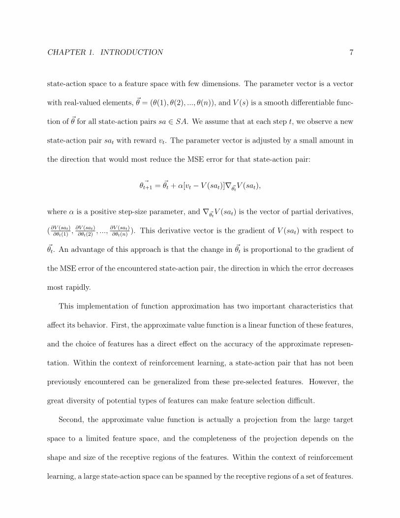
CHAPTER 1. INTRODUCTION 7
state-action space to a feature space with few dimensions. The parameter vector is a vector
with real-valued elements, ~θ = (θ(1), θ(2), ..., θ(n)), and V (s) is a smooth differentiable func-
tion of ~θ for all state-action pairs sa ∈ SA. We assume that at each step t, we observe a new
state-action pair sat with reward vt. The parameter vector is adjusted by a small amount in
the direction that would most reduce the MSE error for that state-action pair:
~θt+1 = ~θt + α[vt − V (sat)]∇~θtV (sat),
where α is a positive step-size parameter, and ∇~θtV (sat) is the vector of partial derivatives,
(∂V (sat)∂θt(1)
, ∂V (sat)∂θt(2)
, ..., ∂V (sat)∂θt(n)
). This derivative vector is the gradient of V (sat) with respect to
~θt. An advantage of this approach is that the change in ~θt is proportional to the gradient of
the MSE error of the encountered state-action pair, the direction in which the error decreases
most rapidly.
This implementation of function approximation has two important characteristics that
affect its behavior. First, the approximate value function is a linear function of these features,
and the choice of features has a direct effect on the accuracy of the approximate represen-
tation. Within the context of reinforcement learning, a state-action pair that has not been
previously encountered can be generalized from these pre-selected features. However, the
great diversity of potential types of features can make feature selection difficult.
Second, the approximate value function is actually a projection from the large target
space to a limited feature space, and the completeness of the projection depends on the
shape and size of the receptive regions of the features. Within the context of reinforcement
learning, a large state-action space can be spanned by the receptive regions of a set of features.

CHAPTER 1. INTRODUCTION 8
Features with large regions can give wide generalization, but might make the representation
of the approximation function coarser and perform only rough discrimination. Features with
small regions can give narrow generalization, but might cause many states to be out of the
receptive regions of all features. Selecting the shape and size of the receptive regions is often
difficult for particular application domains.
A range of function approximation techniques has been studied in recent years. These
techniques can be partitioned into three types, according to the two characteristics described
above: function approximation using natural features, function approximation using basis
functions, and function approximation using Sparse Distribution Memory (SDM).
1.2.1 Function Approximation Using Natural Features
For each application domain, there are natural features that can describe a state. For
example, in some pursuit problems in the grid world, we might have features for location,
vision scale, memory size, communication mechanisms, etc. Choosing such natural features
as the components of the feature vector is an important way to add prior knowledge to a
function approximator.
In function approximation using natural features, the θ-value of a feature indicates
whether the feature is present. The θ-value is constant across the features’ receptive re-
gion and falls sharply to zero at the boundary. These receptive regions may be overlapped.
A large region may give a wide but coarse generalization while a small region may give a
narrow but fine generalization.

CHAPTER 1. INTRODUCTION 9
The advantage of function approximation using natural features is that the representa-
tion of the approximate function is simple and easy to understand. The natural features
can be selected manually and their receptive regions can be adjusted based on the designer’s
intuition. A limitation of this function approximation technique is that it cannot handle
continuous state-action spaces or state-action spaces with high dimensionality. For natural-
feature-based function approximation techniques, the number of features has the largest
effect on the discrimination ability of the approximate function. Increasing the number of
features gives finer discrimination of the state-action space, but may also increase the com-
putational complexity of the algorithm. In general, more features are needed to accurately
approximate continuous state-action spaces and state-action spaces with high dimensionality,
and the number of these needed features grows exponentially with the number of dimensions
in the state-action space [34].
A typical function approximation technique using natural features is Tile Coding [6]. This
approach, which is an extension of coarse coding [20], is also known as ”Cerebellar Model
Articulator Controller,” or CMAC [6]. In Tile Coding, k tilings are selected, each of which
partitions the state-action space into tiles. The receptive field of each feature corresponds
to a tile, and a θ-value is maintained for each tile. A state-action pair p is adjacent to a
tile if the receptive field of the tile includes p. The Q-value of a state-action pair is equal
to the sum of the θ-values of all adjacent tiles. In binary Tile Coding, which is used when
the state-action space consists of discrete values, each tiling corresponds to a subset of the
bit positions in the state-action space and each tile corresponds to an assignment of binary
CHAPTER 1. INTRODUCTION 10
values to the selected bit positions.
1.2.2 Function Approximation Using Basis Functions
For certain problems, a more accurate approximation is obtained if θ-values can vary contin-
uously and represent the degree to which a feature is present. A basis function can be used to
compute such continuously varying θ-values. Basis functions can be designed manually and
the approximate value function is a function of these basis functions. In this case, function
approximation uses basis functions to evaluate the presence of every feature, then linearly
weights these values.
In function approximation with basis functions, the receptive region of a feature depends
on the parameters of the basis function of that feature. These parameters can control the
size, shape and intensity of the receptive region. In general, the θ-value of a feature can vary
across the feature’s receptive region.
An advantage of function approximation with basis function is that the approximated
function is continuous and flexible. The basis functions, each with its own parameters,
give a more precise representation of the value function across the entire state-action space.
However there are two limitations of this function approximation technique. The first is that
selecting these basis functions parameters is difficult in general [38, 17, 34]. The coefficients
of the function combination are often learned by training the solver using test instances,
while the parameters of the basis functions themselves are tuned manually. [34]. When the
number of dimensions of the state and action space is very large, such manual tuning can

CHAPTER 1. INTRODUCTION 11
be difficult.
The second difficulty is that basis function cannot handle state-action spaces with high
dimensionality. It has been found to be hard to apply to continuous problems with more
than 10 − 12 dimensions because of the difficulty of manually tuning the basic functions
[31, 25]. Also, the number of basis functions needed to approximate a state-action space can
be exponential in the number of dimensions, causing the number of basis functions needed
to be very large for a state-action space with high dimensionality.
A typical function approximation technique using basis function is Radial Base Function
Networks (RBFNs) [38]. In an RBFN, a sequence of Gaussian curves is selected as the basis
functions of the features. Each basis function ~φi for a feature i has a center ci, and width
σi. Given an arbitrary state-action pair s, the Q-value of the state-action pair with respect
to the feature i is:
φi(s) = e−||s−ci||
2
2σ2 .
The total Q-value of the state-action pair with respect to all features is the sum of the values
of φi(s) across all features.
A radial basis function is actually a real-valued function whose value depends only on
the distance from its center. It also can be considered a fuzzy membership function, and
in this sense RBFNs represent a fuzzy function approximation technique. But RBFNs are
the natural generalization of coarse coding with binary features to continuous features. A
typical RBF feature unavoidably represents information about some, but not all, dimensions
of the state-action space. This limits RBFNs from approximating large-scale, high-dimension
CHAPTER 1. INTRODUCTION 12
state-action spaces efficiently.
1.2.3 Function Approximation Using SDM
Function approximation using either natural features or basis functions is known to not scale
well for large problem domains, or to require prior knowledge [39, 38, 25]. This approach
is not well-suited to problem domains with high dimensionality. We instead seek a class of
features that can construct approximation functions without restricting the dimensionality
of the state and action space. The theory of Spare Distributed Memory (SDM) [23] gives
such a class of features. These features are often not natural features. They are typically a
set of state-action pairs chosen from the entire state and action space.
In function approximation using SDM, each receptive region is typically defined using
a distance threshold with respect to the location of the feature in the state-action space.
The θ-value of a state-action pair with respect to a feature is constant within the feature’s
receptive region, and is zero outside of this region.
An advantage of function approximation using SDM structure is that its structure is
particularly well-suited to problem domains with high dimensionality. Its computational
complexity depends entirely on the number of prototypes, which is not a function of the
number of the dimensions of the state-action space.
A limitation of this technique is that more prototypes are needed to approximate state-
action spaces for complex problem domains, and the efficiency of function approximation
using SDM is sensitive to the number of the prototypes [25]. Even when enough prototypes

CHAPTER 1. INTRODUCTION 13
are used, the performance of the reinforcement learner with SDM is often poor and unstable
[38, 26, 34]. There is no known mechanism to guarantee the convergence of the algorithm.
Kanerva Coding [24] is the implementation of SDM in function approximation for rein-
forcement learning. Here, a collection of prototype state-action pairs (prototypes), is selected,
each of which corresponds to a binary feature. A state-action pair and a prototype are said
to be adjacent if their bit-wise representations differ by no more than a threshold number
of bits. A state-action pair is represented as a collection of binary features, each of which
equals 1 if and only if the corresponding prototype is adjacent. A value θ(i) is maintained
for each prototype, and an approximation of the value of a state-action pair is then the sum
of the θ-values of the adjacent prototypes. In this way, Kanerva Coding can greatly reduce
the size of the value table that needs to be stored.
1.3 Our Application Domain
In the dissertation, we apply our study to solve the instances from two application domain.
These two domains are predator-prey pursuit domain and cognitive radio network.
The predator-prey pursuit domain [28], introduced in 1986, is a classic example of a
multi-agent system. Problems based on this domain have been solved using a wide variety
of approaches [19, 42, 3, 21] and it also has many different versions that can be used to
illustrate different multi-agent scenarios [34, 36, 37].
A general version of the predator-prey pursuit domain takes place on a rectangular grid
with one or more predator agents and one or more prey agents. Each grid cell is either open

CHAPTER 1. INTRODUCTION 14
or closed, and an agent can only occupy open cells. Each agent has an initial position. The
problem is played in a sequence of time periods. In each time period, each agent can move
to a neighboring open cell one horizontal or vertical step from its current location, or it can
remain in its current cell. All moves are assumed to occur simultaneously, and more than
one predator agent may not occupy the same cell at the same time. The goal of the predator
agents is to capture the prey agents in the shortest time.
The domain can be fully specified by selecting different numbers of predators and prey,
defining capture in different ways, and setting each agent’s visible range. The pursuit domain
is usually studied with two or more predators and one prey; capture occurs when a predator
agent is in the same cell as a prey agent or all predator agents surround a prey agent; the
agent’s visible range may be global or local (limited).
Pursuit problems are difficult to solve in general and problems similar to ours have
been proven to be NP-Complete [8, 33]. Researchers have used approaches such as genetic
algorithms [19] and reinforcement learning [42] to develop solutions. Closed-form solutions
to restricted versions of the problem have been found [3, 21], but most such problems remain
open.
The cognitive radio network domain [30], introduced in 1999, is a novel paradigm of
wireless communication. The basic idea is that the unlicensed devices (also called cognitive
radio users) need to vacate the band once the licensed devices (also known as primary
users) are detected. CR networks impose a great challenge due to the high fluctuation in
the available spectrum as well as diverse quality-of-service (QoS) requirements. Specifically
CHAPTER 1. INTRODUCTION 15
in cognitive radio ad-hoc networks, the distributed multi-hop architecture, the dynamic
network topology, and the time and location varying spectrum availability are some of the
key distinguishing factors.
As the CR network must appropriately choose its transmission parameters based on
limited environmental information, it must be able to learn from its experience, and adapt its
functioning. The challenge necessitates novel design techniques that simultaneously integrate
theoretical research on reinforcement learning and multi-agent interaction with systems level
network design.
1.4 Dissertation Outline
In Chapter 2, we discuss the effectiveness of common function approximation techniques for
large-scale problems. In particular, we first show empirically that the performance of rein-
forcement learners with traditional function approximation techniques over the predator-prey
pursuit domain is poor. We then demonstrate that uneven feature distribution can cause poor
performance and describe a class of adaptive mechanisms that dynamically delete and gen-
erate features for reducing the uneven feature distribution. Finally, we propose our adaptive
Kanerva-based function approximation, which is a form of probabilistic prototype deletion
plus prototype splitting, and show that using adaptive function approximation results in
better learning performance compared to traditional function approximation.
In Chapter 3, we evaluate a class of hard instances of the predator-prey pursuit problem.
We show that the performance using adaptive function approximation is still poor, and

CHAPTER 1. INTRODUCTION 16
argue that this performance is a result of frequent prototype collisions. We show that
dynamic prototype allocation and adaptation can partially reduce these collisions and give
better results than traditional function approximation. To completely eliminate prototype
collisions, we describe a novel fuzzy approach to Kanerva-based function approximation
which uses a fine-grained fuzzy membership grade to describe a state-action pair’s adjacency
with respect to each prototype. This approach, coupled with adaptive prototype allocation,
allows the solver to distinguish membership vectors and reduce the collision rate. We also
show that reducing the similarity between the membership vectors of state-action pairs
can give better results. We use Maximum Likelihood Estimation to adjust the variance of
basis functions and tune the receptive fields of prototypes. Finally, we conclude that our
adaptive fuzzy Kanerva approach with prototype tuning gives better performance than the
pure adaptive Kanerva algorithm.
In Chapter 4, we observe that inappropriate number of prototypes may cause unstable
and poor performance of the solver on the hardest class of pursuit instances, and show that
choosing an optimal number of prototypes can improve the efficiency of function approxima-
tion. We use the theory of rough sets to measure how closely an approximate value function
is approximating the true value function and determines whether or not more prototypes are
required. We show that the structure of equivalence classes induced by prototypes is the key
indicator of the effectiveness of a Kanerva-based reinforcement learner. We then describe
a rough sets-based approach to selecting prototypes. This approach eliminates unneces-
sary prototypes by replacing original prototype set with its reduct, and reduces prototype

CHAPTER 1. INTRODUCTION 17
collisions by splitting equivalence classes with two or more state-action pairs. Finally, we
conclude that rough sets-based Kanerva coding can adaptively select an effective number
of prototypes and greatly improve a Kanerva-based reinforcement learner’s ability to solve
large-scale problems.
In Chapter 5, we apply reinforcement learning with Kanerva-based function approxima-
tion to solve the real-world application of Wireless cognitive radio (CR). Wireless cognitive
radio is a newly emerging paradigm that attempts to opportunistically transmit in licensed
frequencies without affecting the pre-assigned users of these bands. To enable this func-
tionality, such a radio must predict its operational parameters, such as transmit power and
spectrum. These tasks, collectively called spectrum management, are difficult to achieve in a
dynamic distributed environment in which CR users may only make local decisions, and react
to environmental changes. In order to evaluate the efficiency of multi-agent reinforcement
learning-based spectrum management, we first investigate various real-world scenarios and
compare the communication performance using different sets of learning parameters. Our re-
sults indicate that the requirement of RL-based approaches that an estimated value be stored
for every state greatly limits the size and complexity of CR networks that can be solved. We
therefore apply Kanerva-based function approximation to improve our approach’s ability to
handle large cognitive radio networks and evaluate its effect on communication performance.
We conclude that spectrum management based on reinforcement learning with function ap-
proximation can significantly reduce the interference to the licensed users, while maintaining
a high probability of successful transmissions in a cognitive radio ad hoc network.

Chapter 2
Adaptive Function Approximation
Learning problems with large state spaces, such as multi-agent problems, can be difficult
to solve. When applying reinforcement learning to such problems, the size of the table
needed to store the state-action values can limit the complexity of the problems that can be
solved. Function approximation can reduce the size of the table by storing an approximation
of the entire table. Most reinforcement learners behave poorly when used with function
approximation in domains that are very large, have high dimension, or that have a continuous
state-action space [11, 27, 34].
In this chapter, we discuss the effectiveness of common function approximation techniques
for large-scale problems. We first describe the performance of reinforcement learners with
Tile Coding and Kanerva Coding over the predator-prey pursuit domain. We then show
that uneven feature distribution can cause poor performance. We describe a class of adaptive
mechanisms that dynamically delete and generate features based on feature visit frequencies.
18

CHAPTER 2. ADAPTIVE FUNCTION APPROXIMATION 19
Finally, we demonstrate that using adaptive function approximation results in better learning
performance compared to traditional function approximation.
2.1 Experimental Evaluation: Traditional Function Ap-
proximation
Tile Coding and Kanerva Coding are two typical function approximation techniques that
have been widely studied in various application domains [6, 24, 25, 38]. Both techniques give
good learning performance and fast convergence for some instances with small state-action
spaces. However, some empirical results also indicate that reinforcement learners with Tile
Coding or Kanerva Coding may still perform poorly as the size of the state-action space
grows or when applied to hard instances. [26, 34]. We therefore investigate the efficiency of
traditional function approximation as the size of the state-action space increases.
2.1.1 Application Instances
We evaluate the efficiency of traditional function approximation techniques by applying them
to the predator-prey pursuit domain. The domain was selected because: it is a well-known
reinforcement learning problem; there is a class of instances with varying levels of difficulty;
and most importantly, the size of state-action space for solving instances in this domain can
be easily extended.
CHAPTER 2. ADAPTIVE FUNCTION APPROXIMATION 20
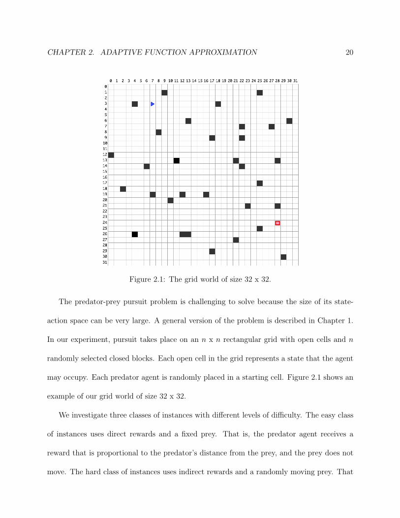
Figure 2.1: The grid world of size 32 x 32.
The predator-prey pursuit problem is challenging to solve because the size of its state-
action space can be very large. A general version of the problem is described in Chapter 1.
In our experiment, pursuit takes place on an n x n rectangular grid with open cells and n
randomly selected closed blocks. Each open cell in the grid represents a state that the agent
may occupy. Each predator agent is randomly placed in a starting cell. Figure 2.1 shows an
example of our grid world of size 32 x 32.
We investigate three classes of instances with different levels of difficulty. The easy class
of instances uses direct rewards and a fixed prey. That is, the predator agent receives a
reward that is proportional to the predator’s distance from the prey, and the prey does not
move. The hard class of instances uses indirect rewards and a randomly moving prey. That
CHAPTER 2. ADAPTIVE FUNCTION APPROXIMATION 21
is, the predator agent receives a reward of 1 when it reaches the cell the prey is occupying,
and receives a reward of 0 in every other cell. The predator attempts to catch a prey that is
moving randomly.
We use Q-learning with traditional Tile Coding and Kanerva Coding to solve the three
classes of pursuit instances on an n x n grid. The size of the grid varies from 8x8 to 32x32.
In each epoch, we apply each learning algorithm to 40 random training instances followed by
40 random test instances. The exploration rate ε is set to 0.3, which we found experimentally
to give the best results in our experiments. The initial learning rate α is set to 0.8, and it is
decreased by a factor of 0.995 after each epoch. For every 40 epochs, we record the average
fraction of test instances solved during those epochs within 2n moves. Each experiment is
performed 3 times and we report the means and standard deviations of the recorded values.
In our experiments, all runs were found to converge within 2000 epochs.
2.1.2 Performance Evaluation of Traditional Tile Coding
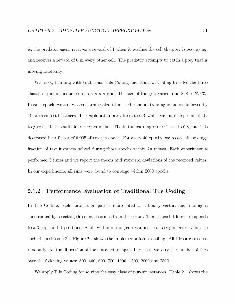
In Tile Coding, each state-action pair is represented as a binary vector, and a tiling is
constructed by selecting three bit positions from the vector. That is, each tiling corresponds
to a 3-tuple of bit positions. A tile within a tiling corresponds to an assignment of values to
each bit position [48].. Figure 2.2 shows the implementation of a tiling. All tiles are selected
randomly. As the dimension of the state-action space increases, we vary the number of tiles
over the following values: 300, 400, 600, 700, 1000, 1500, 2000 and 2500.
We apply Tile Coding for solving the easy class of pursuit instances. Table 2.1 shows the
CHAPTER 2. ADAPTIVE FUNCTION APPROXIMATION 22
Binary vector
000
001
010
011
100
101
110
111
000
001
010
011
100
101
110
111
Each tiling partitions the state-action space
A tiling is constructed by selecting three bit positions.
A tile is an assignment of values to each bit position
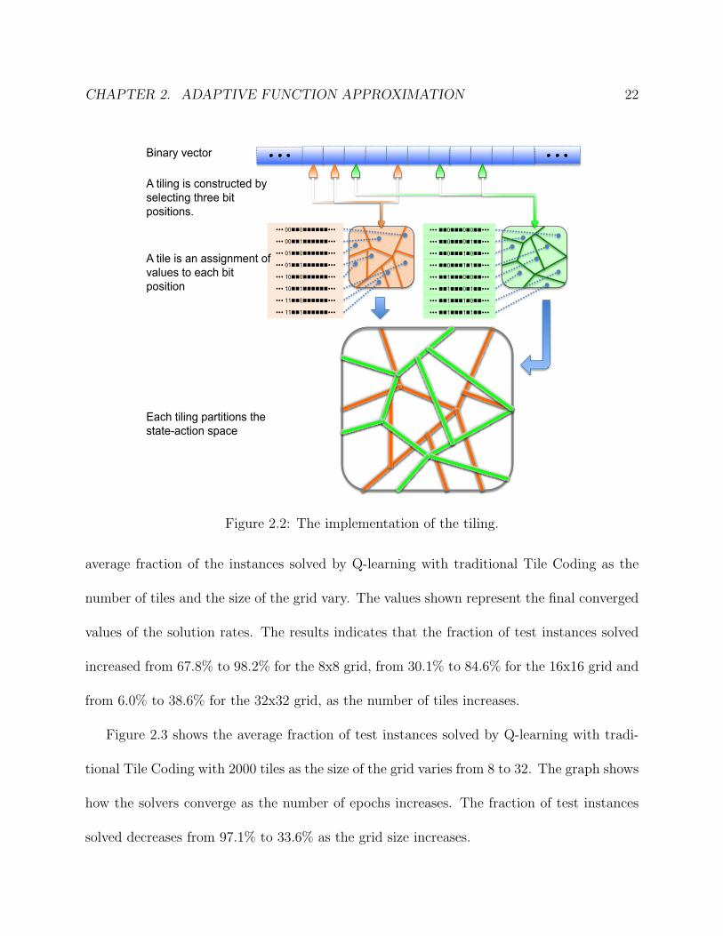
Figure 2.2: The implementation of the tiling.
average fraction of the instances solved by Q-learning with traditional Tile Coding as the
number of tiles and the size of the grid vary. The values shown represent the final converged
values of the solution rates. The results indicates that the fraction of test instances solved
increased from 67.8% to 98.2% for the 8x8 grid, from 30.1% to 84.6% for the 16x16 grid and
from 6.0% to 38.6% for the 32x32 grid, as the number of tiles increases.
Figure 2.3 shows the average fraction of test instances solved by Q-learning with tradi-
tional Tile Coding with 2000 tiles as the size of the grid varies from 8 to 32. The graph shows
how the solvers converge as the number of epochs increases. The fraction of test instances
solved decreases from 97.1% to 33.6% as the grid size increases.

CHAPTER 2. ADAPTIVE FUNCTION APPROXIMATION 23
Table 2.1: The average fraction of test instances solved by Q-learning with traditional TileCoding.
# of Prot. 8x8 16x16 32x32
300 67.8% 30.1% 6.0%400 69.2% 47.6% 9.9%600 75.3% 51.7% 17.2%700 81.3% 56.5% 20.1%1000 90.7% 64.4% 24.7%1500 94.9% 71.1% 29.3%2000 97.1% 80.9% 33.6%2500 98.2% 84.6% 38.6%
0.00
0.10
0.20
0.30
0.40
0.50
0.60
0.70
0.80
0.90
1.00
0 200 400 600 800 1000 1200 1400 1600 1800 2000
Aver
age
solu
tion
rate
Epoch
8X 8 Grid 16X16 Grid 32X32 Grid
Figure 2.3: The fraction of test instances solved by Q-Learning with traditional Tile Codingwith 2000 tiles.
These results show that as the size of the grid varies from 8x8 to 32x32, the fraction of
test instances solved decreases sharply using traditional Tile Coding across all number of
tiles. The number of the tiles used across all sizes of grids has a large effect on the fraction
of test instances solved.

CHAPTER 2. ADAPTIVE FUNCTION APPROXIMATION 24
Prototype #1
Each receptive region partitions the state-action space
Each prototype has its own receptive region.
Prototype #2
Prototype #3
Figure 2.4: The implementation of Kanerva Coding.
2.1.3 Performance Evaluation of Traditional Kanerva Coding
We evaluate traditional Kanerva Coding by varying the number of prototypes and the size
of the grid. We implement Kanerva Coding by representing the state-action pair as a binary
vector. Each entry in the binary vector equals 1 if and only if the corresponding prototype
is adjacent. Every prototype is a randomly selected state-action pair. Figure 2.4 shows the
implementation of the Kanerva Coding. As the dimension of the state-action space increases,
we vary the number of prototypes from 300 to 2500.
We compare Kanerva Coding to Tile Coding when the number of prototypes is same
as the number of tiles. Table 2.2 shows the average fraction of test instances solved by
CHAPTER 2. ADAPTIVE FUNCTION APPROXIMATION 25
Table 2.2: The average fraction of test instances solved by Q-learning with traditional Kan-erva Coding.
# of Traditional Tile Traditional KanervaPrototype 8x8 16x16 32x32 8x8 16x16 32x32
300 67.8% 30.1% 6.0% 57.2% 28.5% 7.9%400 69.2% 47.6% 9.9% 63.5% 36.7% 13.2%600 75.3% 51.7% 17.2% 75.0% 42.3% 22.3%700 81.3% 56.5% 20.1% 79.2% 47.2% 28.0%1000 90.7% 64.4% 24.7% 90.9% 50.3% 32.1%1500 94.9% 71.1% 29.3% 91.4% 59.1% 36.6%2000 97.1% 80.9% 33.6% 93.1% 75.4% 40.6%2500 98.2% 84.6% 38.6% 93.5% 82.3% 43.2%
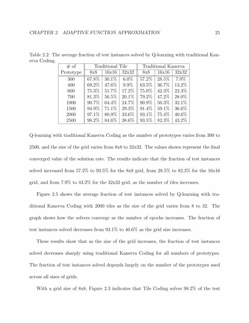
Q-learning with traditional Kanerva Coding as the number of prototypes varies from 300 to
2500, and the size of the grid varies from 8x8 to 32x32. The values shown represent the final
converged value of the solution rate. The results indicate that the fraction of test instances
solved increased from 57.2% to 93.5% for the 8x8 grid, from 28.5% to 82.3% for the 16x16
grid, and from 7.9% to 43.2% for the 32x32 grid, as the number of tiles increases.
Figure 2.5 shows the average fraction of test instances solved by Q-learning with tra-
ditional Kanerva Coding with 2000 tiles as the size of the grid varies from 8 to 32. The
graph shows how the solvers converge as the number of epochs increases. The fraction of
test instances solved decreases from 93.1% to 40.6% as the grid size increases.
These results show that as the size of the grid increases, the fraction of test instances
solved decreases sharply using traditional Kanerva Coding for all numbers of prototypes.
The fraction of test instances solved depends largely on the number of the prototypes used
across all sizes of grids.
With a grid size of 8x8, Figure 2.3 indicates that Tile Coding solves 98.2% of the test
CHAPTER 2. ADAPTIVE FUNCTION APPROXIMATION 26
0.00
0.10
0.20
0.30
0.40
0.50
0.60
0.70
0.80
0.90
1.00
0 200 400 600 800 1000 1200 1400 1600 1800 2000
Aver
age
solu
tion
rate
Epoch
8X 8 Grid
16X16 Grid
32X32 Grid
Figure 2.5: The fraction of test instances solved by Q-Learning with traditional KanervaCoding with 2000 prototypes.
instances while Kanerva Coding solves only 93.5% of the test instances, after 2000 epochs.
However, for a grid size of 32x32, Tile Coding solves 33.6% of the test instances while Kanerva
Coding solves 43.2% of the test instances, after 2000 epochs.
These results show that when the number of dimensions is small, traditional Tile Coding
outperforms traditional Kanerva Coding. However, as the number of dimensions increases,
Tile Coding’s performance degrades faster than the performance of Kanerva Coding when
the number of prototypes is fixed. We conclude that Kanerva Coding performs better relative
to Tile Coding when the dimension of the state-action space is large, and for this reason we
choose Kanerva Coding as the starting point for our research.

CHAPTER 2. ADAPTIVE FUNCTION APPROXIMATION 27
2.2 Visit Frequency and Feature Distribution
The performance evaluation in the previous section showed that the efficiency of traditional
function approximation techniques decreases sharply as the size of state-action space in-
creases. Our performance evaluation also showed that the performance of reinforcement
learners with Tile Coding and Kanerva Coding is sensitive to the number of features, that
is, the number of tiles in Tile Coding or the number of prototypes in Kanerva Coding. If
the number of features is small relative to the number of state-action pairs, or if the features
themselves are not well chosen, the approximate values will not be similar to the true values
and the reinforcement learner will give poor results. If the number of features is very large
relative to the number of state-action pairs, each feature may be adjacent to a small number
of state-action pairs. In this case, the approximate state-action values will tend to be close
to the true values, and the reinforcement learner will operate as usual. Unfortunately, we
often do not have enough memory to store a large number of features, so we consider how
to produce the smallest set of features which can span the entire state space.
It is difficult to generate such an optimal set of features for several reasons: the space
of possible subsets is very large and the state-action pairs encountered by the solver depend
on the specific problem instance being solved. We therefore investigate several heuristic
solutions to the feature optimization problem.
We say that a feature is visited during Q-learning if it is adjacent to the current state-
action pair. Intuitively speaking, if a specific feature is rarely visited, it implies that few
state-action pairs are adjacent to the feature. This suggests that the feature is inappropriate

CHAPTER 2. ADAPTIVE FUNCTION APPROXIMATION 28
for the particular application. In contrast, if a specific feature is visited frequently, it implies
that many state-action pairs are adjacent to the feature. This suggests that the feature
may not distinguish many distinct state-action pairs. Therefore, prototypes that are rarely
visited do not contribute to the solution of instances. Similarly, prototypes that are visited
very frequently are likely to decrease the distinguishability of state-action pairs. Removing
the rarely-visited and heavily-visited prototypes may reduce inappropriate prototypes and
improve the efficiency of Kanerva coding. Our goal is therefore to generate a set of features
where each feature is visited an average number of times.
We define a feature’s visit frequency as the number of visits to the feature during a learning
process. In particular, we refer to a tile’s visit frequency in Tile Coding and a prototype’s
visit frequency in Kanerva Coding. We observe the distribution of visit frequencies across
all tiles or prototypes over a converged learning process.
The frequency distribution of visits to tiles over three sample runs using Q-learning with
Tile Coding is shown in Figure 2.6. The example uses direct rewards, fixed prey, and 2000
tiles. Similarly, the frequency distribution of visits to prototypes over three sample runs
using Q-learning with Kanerva Coding and 2000 prototypes is shown in Figure 2.7. The
non-uniform distribution of visit frequencies across all tiles or prototypes indicates that
most prototypes are either frequently visited, or rarely visited. In next section, we describe
ways to generate sets of features with visit frequencies that are more uniform.

CHAPTER 2. ADAPTIVE FUNCTION APPROXIMATION 29
0
50
100
150
200
250
1 6 11 16 21 26 31 36 41 46 51
Num
ber o
f Tile
s
Visits
32x32 Grid 16x16 Grid 8x 8 Grid
Figure 2.6: The frequency distribution of visits to tiles over a sample run using Q-learningwith Tile Coding
0
50
100
150
200
250
1 6 11 16 21 26 31 36 41 46 51
Num
ber o
f Pro
toty
pes
Visits
32x32 Grid 16x16 Grid 8x 8 Grid
Figure 2.7: The frequency distribution of visits to prototypes over a sample run using Q-learning with Kanerva Coding

CHAPTER 2. ADAPTIVE FUNCTION APPROXIMATION 30
2.3 Adaptive Mechanism in Kanerva-Based Function
Approximation
The goal of feature optimization for function approximation is to produce a set of features
where visit frequencies across feature are relatively uniform. The visit frequency of a fea-
ture is equal to the number of adjacent state-action pairs encountered during a learning
process. The specific state-action pairs encountered by the solver depend on the specific
problem instance being solved. Therefore, adaptively choosing features appropriate to the
particular application is an important way to implement feature optimization for function
approximation.
Feature adaptation uses prior knowledge and online experience to improve a reinforcement
learner. There have been few published attempts to explore this type of algorithm [34] and
no known attempts to evaluate and improve the quality of feature adaptation for function
approximation.
We optimize features using visit frequencies. We divide the original features into three
categories: features with a low visit frequency, features with a high visit frequency, and the
rest of the features.
We describe and evaluate four optimization mechanisms to optimize the set of fea-
tures. Since Kanerva Coding outperforms Tile Coding when the state-action space is high-
dimensional, we base our optimization mechanisms on Kanerva Coding. Initial prototypes
are selected randomly from the entire space of possible state-action pairs. Q-learning with

CHAPTER 2. ADAPTIVE FUNCTION APPROXIMATION 31
Kanerva Coding is used to develop policies for the predator agents, while keeping track of
the number of visits to each prototype. After a fixed number of iterations, we update the
prototypes using the mechanisms described below.
2.3.1 Prototype Deletion and Generation
Prototypes that are rarely visited do not contribute to the solution of instances. Similarly,
prototypes that are visited very frequently are likely to decrease the distinguishability of
state-action pairs. It makes sense to delete both types of prototypes and replace them with
new prototypes whose visit frequencies are closer to an average value.
In our implementation, we periodically delete a fraction of the prototypes whose visit
frequencies are lowest, and a fraction of the prototypes whose visit frequency are highest.
The fraction of prototypes that is deleted slowly decreases as the algorithm runs. The θ-value
and visit frequency of the new prototype are initially set to zero. We refer to this approach
as deterministic prototype deletion.
An advantage of this approach is that it is easy to implement and it uses application- and
instance-specific information to guide the deletion of rarely or frequently visited prototypes.
However, this approach deletes prototypes deterministically which does not give the solver
the flexibility to keep some prototypes that are rarely or frequently visited. For example, if
the number of prototypes is very large, some prototypes that might become useful will not
be visited in an early epoch and will be deleted.
In order to overcome this disadvantage, we delete prototypes with a probability equal

CHAPTER 2. ADAPTIVE FUNCTION APPROXIMATION 32
to an exponential function of the number of visits. I.e. the probability pdel of deleting a
prototype whose visit frequency is v is pdel = λe−λv, where λ is a parameter that can vary
from 0 to 1. In this approach, prototypes that are rarely visited tend to be deleted with a
high probability, while prototypes that are frequently visited are rarely deleted. We refer to
this approach as probabilistic prototype deletion.
We attempt to replace prototypes that have been deleted with new prototypes that will
tend to improve the behavior of the function approximation. One approach is to generate
new prototypes randomly from the entire state space. While this approach aggressively
searches the state space for useful prototypes, it does not use domain- or instance-specific
information.
We instead create new prototypes by splitting heavily-visited prototypes. A prototype s1
that has been visited the most times is selected, and a new prototype s2 that is a neighbor
of s1 is created by inverting a fixed number of bits in s1. The θ-value and visit frequency
of the new prototype are initially set to zero. The prototype s1 remains unchanged. In this
approach, new prototypes near prototypes with the highest visit frequencies are created.
These prototypes are similar but distinct which tends to reduce the number of visits to
nearby prototypes, and therefore increase the distinguishability of these prototypes. We
refer to this approach as prototype splitting.
Our adaptive Kanerva-based function approximation uses the probabilistic prototype
deletion with prototype splitting. The approach makes the distribution of feature visit
frequencies more uniform. We therefore refer to this approach as frequency-based prototype

CHAPTER 2. ADAPTIVE FUNCTION APPROXIMATION 33
Table 2.3: The average fraction of test instances solved by Q-learning with adaptive KanervaCoding.
# of Grid SizePrototypes 8x8 16x16 32x32
300 81.3% 49.6% 23.3%400 92.3% 52.3% 28.3%600 98.9% 62.4% 37.0%700 99.0% 70.4% 41.7%1000 99.2% 84.5% 62.8%1500 99.3% 95.7% 77.6%2000 99.5% 95.9% 90.5%2500 99.5% 96.1% 92.4%
optimization.
2.3.2 Performance Evaluation of Adaptive Kanerva-Based Func-
tion Approximation
We evaluate our prototype optimization algorithm by applying Q-learning with adaptive
Kanerva Coding to solve the easy class of predator-prey pursuit instances described in Sec-
tion 2.1 on an nxn grid. Prototype optimization is applied after every 20 epochs. The size of
the grid n also varies from 8x8 to 32x32. All others experimental parameters are unchanged.
Table 2.3 shows the average fraction of test instances solved by Q-Learning with adaptive
Kanerva Coding as the number of prototype varies from 300 to 2500, and the size of the
grid varies from 8x8 to 32x32. The values shown represent the final converged values of the
solution rates. The results indicate that the fraction of test instances solved increased from
81.3% to 99.5% for the 8x8 grid, from 49.6% to 96.1% for the 16x16 grid and from 23.3% to
92.4% for the 32x32 grid, as the number of prototypes increases.
CHAPTER 2. ADAPTIVE FUNCTION APPROXIMATION 34
!"#$%&!"#$%&
!"#$%&'(#"%&
'(#"%&
'(#"%&
)&
)%*&
)%+&
)%,&
)%-&
)%.&
)%/&
)%0&
)%1&
)%2&
*&
*& +& ,&
!"#$%&#'()*+,
)-'.%/#'
0$12'(13#'
131& */3*/& ,+3,+&
0.00
0.10
0.20
0.30
0.40
0.50
0.60
0.70
0.80
0.90
1.00
0 200 400 600 800 1000 1200 1400 1600 1800 2000
Av
era
ge
so
luti
on
ra
te
Epoch
(1) 8X 8 Grid, Adaptive (2) 16X16 Grid, Adaptive (3) 8X 8 Grid, Traditional (4) 32X32 Grid, Adaptive (5) 16X16 Grid, Traditional (6) 32X32 Grid, Traditional
!"#$!%#$
!&#$!'#$
!(#$
!)#$
Figure 2.8: The fraction of test instances solved by Q-Learning with adaptive KanervaCoding with 2000 prototypes.
Figure 2.8 shows the average fraction of test instances solved by Q-Learning with adaptive
and traditional Kanerva Coding with 2000 tiles as the size of the grid varies from 8x8
to 32x32. The graph shows how the solvers converge as the number of epochs increases.
The traditional Kanerva algorithm solves approximately 93.1% of the test instances with
a grid size of 8x8, 75.4% with a grid size of 16x16, and 40.6% with a grid size of 32x32.
Adaptive Kanerva algorithm solves approximately 99.5% of the test instances with a grid
CHAPTER 2. ADAPTIVE FUNCTION APPROXIMATION 35
0
50
100
150
200
250
0 5 10 15 20 25 30 35 40 45 50
Num
ber o
f Pro
toty
pes
Visits
32x32 Grid 16x16 Grid 8x 8 Grid
Figure 2.9: The frequency distribution of visits to prototypes over a sample run using Q-learning with adaptive Kanerva Coding.
size of 8x8, 95.9% with a grid size of 16x16, and 90.5% with a grid size of 32x32. These
results indicate that adaptive Kanerva Coding outperforms traditional Kanerva Coding and
that probabilistic prototype deletion with prototype splitting can significantly increase the
efficiency of Kanerva-based function approximation.
We also observe the distribution of visit frequencies across all prototypes after opti-
mization. Figure 2.9 shows these frequency distributions over the same instances used in
Section 2.2. The graph shows that most prototypes are visited an average number of times.
These results indicate that the optimized prototypes correctly span the state-action space of
a particular instance. The results suggest that that the improved performance of the adap-
tive Kanerva algorithm over the traditional algorithm is due to the more uniform frequency
distribution of visits to prototypes.
CHAPTER 2. ADAPTIVE FUNCTION APPROXIMATION 36
2.4 Summary
In this chapter, we evaluated and compared the behavior of two typical function approxima-
tion techniques, Tile Coding and Kanerva Coding, over the predator-prey pursuit domain.
We showed that traditional function approximation techniques applied within a reinforce-
ment learner do not give good learning performance. By exploring the features’ visit fre-
quencies, we revealed that the non-uniform frequency distribution of visits across all features
is a key factor in achieving poor performance.
We then described our new adaptive Kanerva-based function approximation algorithm,
based on prototype deletion and generation. We showed that probabilistic prototype deletion
with prototype splitting increases the fraction of test instances solved. These results demon-
strate that our approach can dramatically improve the quality of the results obtained and
reduce the number of prototypes required. We conclude that adaptive Kanerva Coding using
frequency-based prototype optimization can greatly improve a Kanerva-based reinforcement
learner’s ability to solve large-scale multi-agent problems.

Chapter 3
Fuzzy Logic-based Function
Approximation
Feature optimization can be used to improve the efficiency of traditional function approx-
imation within reinforcement learners to a certain extent. This approach can produce a
uniform frequency distribution of visits across features by deleting features that are not
necessary and splitting important features. In Chapter 2, we described our implementation
of this algorithm using Adaptive Kanerva Coding. However this approach still gives poor
performance, and the improvement over traditional Kanerva Coding is small when applied
to hard instances of large-scale multi-agent systems. We therefore must consider whether
other potential factors are causing this poor performance.
In this chapter, we attempt to solve a class of hard instances in the predator-prey pursuit
domain and argue that the poor performance that we observe is caused by frequent prototype
37

CHAPTER 3. FUZZY LOGIC-BASED FUNCTION APPROXIMATION 38
collisions. We show that feature optimization can give better results by partially reducing
these collisions. We then describe our novel approach, fuzzy Kanerva-based function approx-
imation, that uses a fine-grained fuzzy membership grade to describe a state-action pair’s
adjacency with respect to each prototype. This approach can completely eliminate prototype
collisions.
3.1 Experimental Evaluation: Kanerva Coding Applied
to Hard Instances
In Chapter 2, we described three classes of pursuit instances that ranged in difficulty. Adap-
tive Kanerva Coding, which outperforms tradition Kanerva Coding, gave good learning per-
formance and fast convergence over the easy class of instances. We first evaluate a reinforce-
ment learner with adaptive Kanerva Coding on a collection of hard instances.
We evaluate traditional and adaptive Kanerva Coding by applying them to pursuit in-
stances using indirect rewards and a randomly moving prey. The state-action pairs are
represented as binary vectors and all prototypes are selected randomly. Probabilistic proto-
type deletion with prototype splitting is used as feature optimization for adaptive Kanerva
Coding. The number of prototypes varies over the following values: 300, 400, 600, 700, 1000,
1500, 2000 and 2500. The size of the grid varies from 8x8 to 32x32.
Table 3.1 shows the average fraction of hard test instances solved by Q-learning with
adaptive Kanerva Coding as the number of prototypes and the size of the grid vary. The
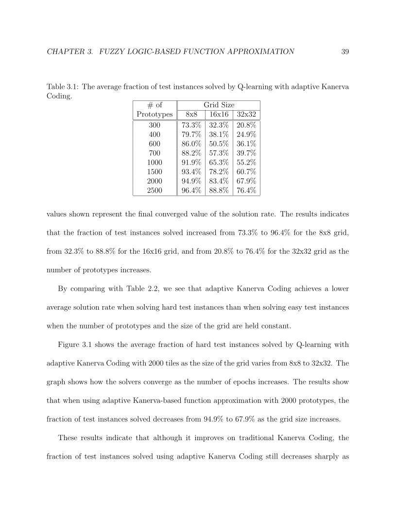
CHAPTER 3. FUZZY LOGIC-BASED FUNCTION APPROXIMATION 39
Table 3.1: The average fraction of test instances solved by Q-learning with adaptive KanervaCoding.
# of Grid SizePrototypes 8x8 16x16 32x32
300 73.3% 32.3% 20.8%400 79.7% 38.1% 24.9%600 86.0% 50.5% 36.1%700 88.2% 57.3% 39.7%1000 91.9% 65.3% 55.2%1500 93.4% 78.2% 60.7%2000 94.9% 83.4% 67.9%2500 96.4% 88.8% 76.4%
values shown represent the final converged value of the solution rate. The results indicates
that the fraction of test instances solved increased from 73.3% to 96.4% for the 8x8 grid,
from 32.3% to 88.8% for the 16x16 grid, and from 20.8% to 76.4% for the 32x32 grid as the
number of prototypes increases.
By comparing with Table 2.2, we see that adaptive Kanerva Coding achieves a lower
average solution rate when solving hard test instances than when solving easy test instances
when the number of prototypes and the size of the grid are held constant.
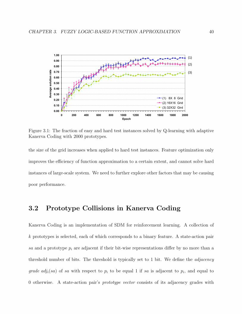
Figure 3.1 shows the average fraction of hard test instances solved by Q-learning with
adaptive Kanerva Coding with 2000 tiles as the size of the grid varies from 8x8 to 32x32. The
graph shows how the solvers converge as the number of epochs increases. The results show
that when using adaptive Kanerva-based function approximation with 2000 prototypes, the
fraction of test instances solved decreases from 94.9% to 67.9% as the grid size increases.
These results indicate that although it improves on traditional Kanerva Coding, the
fraction of test instances solved using adaptive Kanerva Coding still decreases sharply as
CHAPTER 3. FUZZY LOGIC-BASED FUNCTION APPROXIMATION 40
0.00
0.10
0.20
0.30
0.40
0.50
0.60
0.70
0.80
0.90
1.00
0 200 400 600 800 1000 1200 1400 1600 1800 2000
Aver
age
solu
tion
rate
Epoch
(1) 8X 8 Grid (2) 16X16 Grid (3) 32X32 Gird
(1)
(2)
(3)
Figure 3.1: The fraction of easy and hard test instances solved by Q-learning with adaptiveKanerva Coding with 2000 prototypes.
the size of the grid increases when applied to hard test instances. Feature optimization only
improves the efficiency of function approximation to a certain extent, and cannot solve hard
instances of large-scale system. We need to further explore other factors that may be causing
poor performance.
3.2 Prototype Collisions in Kanerva Coding
Kanerva Coding is an implementation of SDM for reinforcement learning. A collection of
k prototypes is selected, each of which corresponds to a binary feature. A state-action pair
sa and a prototype pi are adjacent if their bit-wise representations differ by no more than a
threshold number of bits. The threshold is typically set to 1 bit. We define the adjacency
grade adji(sa) of sa with respect to pi to be equal 1 if sa is adjacent to pi, and equal to
0 otherwise. A state-action pair’s prototype vector consists of its adjacency grades with
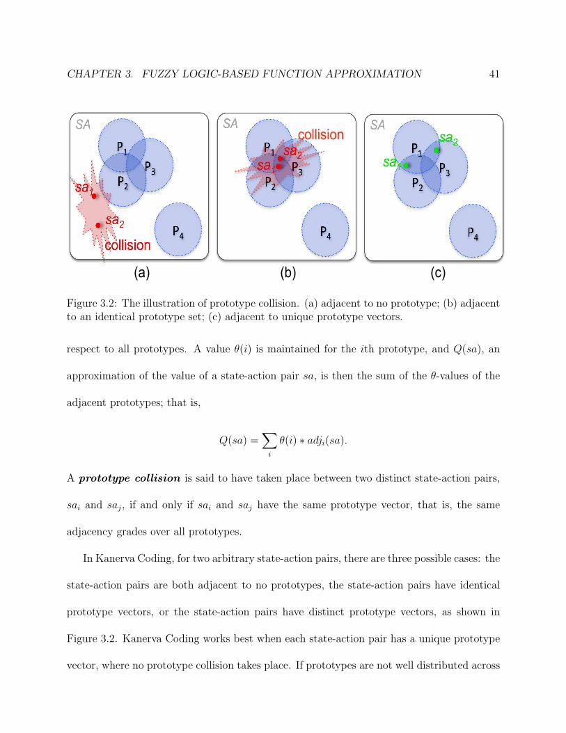
CHAPTER 3. FUZZY LOGIC-BASED FUNCTION APPROXIMATION 41
!"#
!$#
!%#
!&#
sa1
sa2
SA
!"#
!$#
!%#
!&#
sa1
sa2
SA
collision
!"#
!$#
!%#
!&#
sa1 sa
2
SA collision
(a) (b) (c)
Figure 3.2: The illustration of prototype collision. (a) adjacent to no prototype; (b) adjacentto an identical prototype set; (c) adjacent to unique prototype vectors.
respect to all prototypes. A value θ(i) is maintained for the ith prototype, and Q(sa), an
approximation of the value of a state-action pair sa, is then the sum of the θ-values of the
adjacent prototypes; that is,
Q(sa) =∑i
θ(i) ∗ adji(sa).
A prototype collision is said to have taken place between two distinct state-action pairs,
sai and saj, if and only if sai and saj have the same prototype vector, that is, the same
adjacency grades over all prototypes.
In Kanerva Coding, for two arbitrary state-action pairs, there are three possible cases: the
state-action pairs are both adjacent to no prototypes, the state-action pairs have identical
prototype vectors, or the state-action pairs have distinct prototype vectors, as shown in
Figure 3.2. Kanerva Coding works best when each state-action pair has a unique prototype
vector, where no prototype collision takes place. If prototypes are not well distributed across
CHAPTER 3. FUZZY LOGIC-BASED FUNCTION APPROXIMATION 42
the state-action space, many state-action pairs will either not be adjacent to any prototypes,
or adjacent to identical sets of prototypes, corresponding to identical prototype vectors. If
two similar state-action pairs are adjacent to the same set of prototypes, their state-action
value are always same during the learning process. Typically, the solver needs to distinguish
such state-action pairs, which is not possible in this case. Such prototype collisions reduce
the quality of the results, and the estimates of Q-values of such state-action pairs will be
equal [49]..
The collision rate in Kanerva Coding is the fraction of state-action pairs that are
either adjacent to no prototypes, or adjacent to the same set of prototypes as some other
state-action pair. The larger the value of the collision rate, the more frequently prototype
collisions will occur during Kanerva-based function approximation. The prototype collision
is therefore inversely proportional to the learning performance of a reinforcement learner
with Kanerva-based function approximation.
Selecting a set of prototypes that distinguishes frequently-visit distinct state-actions pairs
can improve the solver’s ability to solve the problem. However, it is difficult to generate such a
set of prototypes for several reasons: the space of possible subsets is very large, and the state-
action pairs encountered by the solver depend on the specific problem instance being solved.
Dynamic prototype allocation and adaptation removes unnecessary prototypes and adds
new prototypes that cover parts of the state-action space that are frequently visited during
instance-based learning. In this way, prototypes can be adaptively adjusted to minimize
prototype collisions for the specific problem domain.

CHAPTER 3. FUZZY LOGIC-BASED FUNCTION APPROXIMATION 43
9.4% 0.6%
28.1%
2.8%
43.3%
9.2%
15.6%
7.9%
22.6%
12.3%
28.2%
20.3%
75.0%
91.5%
49.3%
84.9%
28.5%
70.5%
0%
10%
20%
30%
40%
50%
60%
70%
80%
90%
100%
Traditional Adaptive Traditional Adaptive Traditional Adaptive
% o
f Sta
te-a
ctio
n Pa
irs
Grid size
Adjacent to a unique prototype set Adjacent to a non-unique prototype set Adjacent to no prototypes
8X8 16X16 32X32
Figure 3.3: Prototype collisions using traditional and adaptive Kanerva-based function ap-proximation with 2000 prototypes.
In order to evaluate the negative effect of prototype collisions, we observe the collision
rates produced when using traditional Kanerva Coding and adaptive Kanerva Coding as the
size of the grid varies. Figure 3.3 shows the fraction of state-action pairs that are adjacent
to no prototypes, adjacent to identical sets of prototypes, and adjacent to a unique set
of prototypes when traditional Kanerva Coding and adaptive Kanerva Coding with 2000
prototypes are applied to easy predator-prey instances of varying sizes. Here, the collision
rate is the sum of the fraction of state-action pairs that are adjacent to no prototypes and the
fraction of state-action pairs that are adjacent to identical sets of prototypes. These results
show that for the traditional algorithm, the collision rate increases from 25.0% to 71.5% as
the size of grid increases. For the adaptive algorithm space, the collision rate increases from
8.5% to 29.5% as the size of the grid increases.

CHAPTER 3. FUZZY LOGIC-BASED FUNCTION APPROXIMATION 44
The results also suggest that the improved performance of the adaptive Kanerva algo-
rithm over the traditional algorithm occurs with the reduction of prototype collisions. For
example, the adaptive Kanerva algorithm reduces the collision rate from 71.5% to 29.5%
while the average solution rate for the adaptive algorithm increases for a grid size of 32x32.
However, the results also indicate that while the adaptive mechanism successfully reduces
the number of collisions caused by the fraction of state-action pairs that are adjacent to no
prototypes, it is not as successful at reducing the number of collisions caused by the fraction
of state-action pairs that are adjacent to identical sets of prototypes. For example, the
adaptive algorithm reduces the number of collisions caused by state-action pairs that are
adjacent to no prototypes by 91.7% in the 8x8 grid, by 90.0% in the 16x16 grid, and by
78.8% in the 32x32 grid. But it reduces only 49.4% of the collisions caused by the fraction of
state-action pairs that are adjacent to identical sets of prototypes in the grid of 8x8, 45.6%
in the grid of 16x16 and 28.0% in the grid of 32x32.
For further clarify the effect of prototype collisions to the efficiency of Kanerva-based
function approximation, we evaluate the performance of traditional and adaptive Kanerva-
based function approximation and their corresponding collision rates using different number
of prototypes and different sizes of grids. Figure 3.4 shows the fraction of test instances solved
(solution rate) and the fraction of of state-action pairs that are adjacent to no prototypes and
adjacent to identical prototype vectors (collision rate) by traditional and adaptive Kanerva-
based function approximation as the number of prototypes varies from 300 to 2500 in the
grid of varying sizes from 8 to 32.

CHAPTER 3. FUZZY LOGIC-BASED FUNCTION APPROXIMATION 45
0%
20%
40%
60%
80%
100%
300 600 1000 1500 2000 2500
Sol$on Rate
Number of Prototypes
Tradi0onal
Adap0ve
(a) 8 x 8
0%
20%
40%
60%
80%
100%
300 600 1000 1500 2000 2500
CollisionRate
NumberofPrototypes
Adjacenttouniqueprototypeset
Adjacenttoiden;calprototypeset
Adjacenttonoprototype
3006001000150020002500
Tra.Ada.Tra.Ada.Tra.Ada.Tra.Ada.Tra.Ada.Tra.Ada.
(b) 8 x 8
0%
20%
40%
60%
80%
100%
300 600 1000 1500 2000 2500
Sol$on Rate
Number of Prototypes
Tradi0onal
Adap0ve
(c) 16 x 16
0%
20%
40%
60%
80%
100%
300 600 1000 1500 2000 2500
CollisionRate
NumberofPrototypes
Adjacenttouniqueprototypeset
Adjacenttoiden;calprototypeset
Adjacenttonoprototype
3006001000150020002500
Tra.Ada.Tra.Ada.Tra.Ada.Tra.Ada.Tra.Ada.Tra.Ada.
(d) 16 x 16
0%
20%
40%
60%
80%
100%
300 600 1000 1500 2000 2500
Sol$on Rate
Number of Prototypes
Tradi0onal
Adap0ve
(e) 32 x 32
0%
20%
40%
60%
80%
100%
300 600 1000 1500 2000 2500
CollisionRate
NumberofPrototypes
Adjacenttouniqueprototypeset
Adjacenttoiden;calprototypeset
Adjacenttonoprototype
3006001000150020002500
Tra.Ada.Tra.Ada.Tra.Ada.Tra.Ada.Tra.Ada.Tra.Ada.
(f) 32 x 32
Figure 3.4: Average fraction of test instances solved (solution rate) (a) 8x8 grid; (c) 16x16grid; (e) 32x32 grid, and the fraction of of state-action pairs that are adjacent to no pro-totypes and adjacent to identical prototype vectors (collision rate) (b) 8x8 grid; (d) 16x16grid; (f) 32x32 grid by traditional and adaptive Kanerva-based function approximation asthe number of prototypes varies from 300 to 2500.

CHAPTER 3. FUZZY LOGIC-BASED FUNCTION APPROXIMATION 46
The values shown represent the final converged value of the solution rate. The results
show that, when using traditional Kanerva Coding, the solution rate increases from 57.2%
to 93.5% while the collision rate decreases from 83.7% to 22.9% for the 8x8 grid, the solution
rate increases from 28.5% to 82.3% while the collision rate decreases from 65.7% to 48.4%
for the 16x16 grid and the solution rate increases from 7.9% to 43.2% while the collision rate
decreases from 89.7% to 70.8% for the 32x32 grid, as the number of prototypes increases. As
a comparison, when using adaptive Kanerva Coding, the solution rate increases from 81.3%
to 99.5% while the collision rate decreases from 50.0% to 8.8% for the 8x8 grid, the solution
rate increases from 49.6% to 96.1% while the collision rate decreases from 65.7% to 16.2% for
the 16x16 grid and the solution rate increases from 23.3% to 92.4% while the collision rate
decreases from 84.9% to 25.4% for the 32x32 grid, as the number of prototypes increases.
These results indicate that the fraction of test instances solved decreases sharply while the
collision rate increases sharply using both traditional and adaptive Kanerva-based function
approximation with different number of prototypes across all sizes of grids. The results also
indicate that adaptive Kanerva Coding has better learning performance and causes fewer
prototype collisions over traditional Kanerva Coding and the tendency is magnified as the
size of grid increases .
However, the performance of the adaptive algorithm on large instances is still poor as the
number of prototypes decreases, as shown in Figure 3.4. It is therefore necessary to consider
a more effective approach for reducing the collision rate as the dimension of the state-action
space increases.

CHAPTER 3. FUZZY LOGIC-BASED FUNCTION APPROXIMATION 47
3.3 Adaptive Fuzzy Kanerva Coding
A more flexible and powerful approach to function approximation is to allow a state-action
pair to update θ-values of all prototypes, instead of a subset of neighbor prototypes. Instead
of being binary values, we use fuzzy membership grades that vary continuously between 0
and 1 across all prototypes. Such fuzzy membership grades are larger for closer prototypes
and smaller for more distant prototypes. Since prototype collisions occur only when two
state-action pairs have the same real values in all elements of their membership vectors,
collisions are less likely.
In the traditional Kanerva Coding, a collection of k prototypes is selected. A state-
action pair sa and a prototype pi are said to be adjacent if their bit-wise representations
differ by no more than a threshold number of bits. To introduce fuzzy membership grades,
we reformulate this definition of traditional Kanerva Coding using fuzzy logic [16, 13, 44].
We define the membership grade µi(sa) of s with respect to pi
µi(sa) =
1 if sa is adjacent to pi,
0 otherwise.
A state-action pair’s membership vector consists of its membership grades with respect to
all prototypes. A value θ(i) is maintained for the ith feature, and Q̂(sa), an approximation of
the value of a state-action pair sa, is then the sum of the θ-values of the adjacent prototypes.
That is
Q̂(sa) =∑i
θ(i)µi(sa).
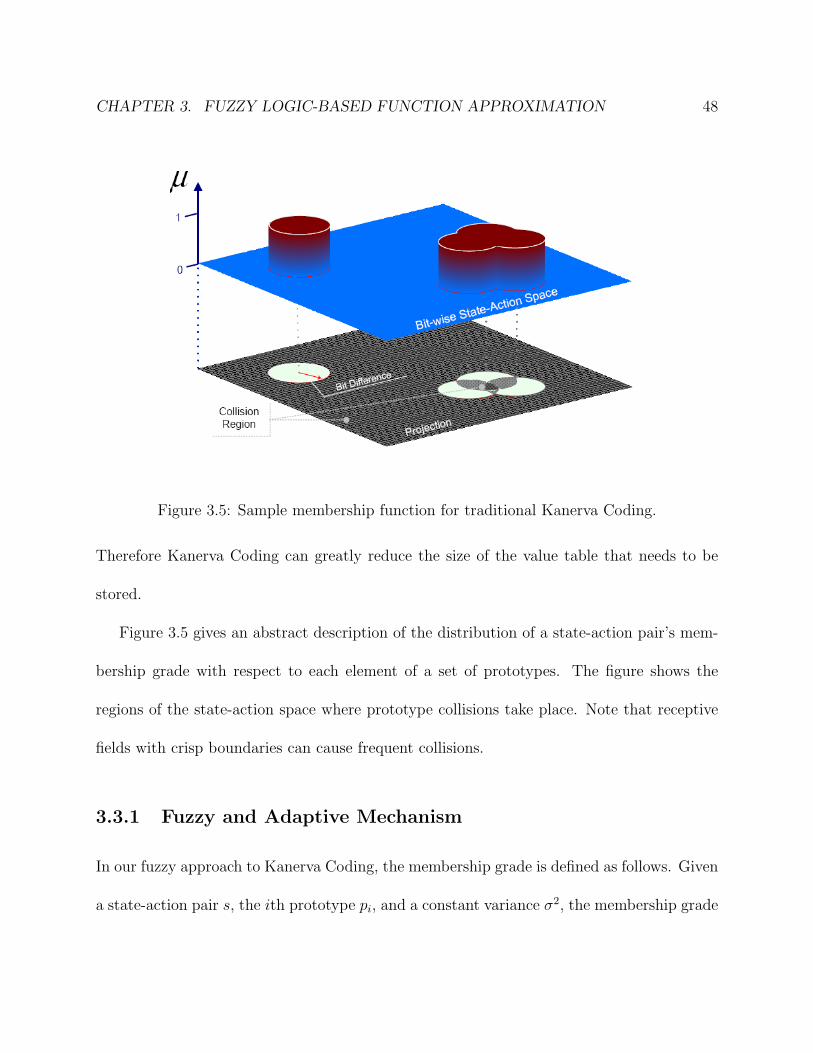
CHAPTER 3. FUZZY LOGIC-BASED FUNCTION APPROXIMATION 48
Figure 3.5: Sample membership function for traditional Kanerva Coding.
Therefore Kanerva Coding can greatly reduce the size of the value table that needs to be
stored.
Figure 3.5 gives an abstract description of the distribution of a state-action pair’s mem-
bership grade with respect to each element of a set of prototypes. The figure shows the
regions of the state-action space where prototype collisions take place. Note that receptive
fields with crisp boundaries can cause frequent collisions.
3.3.1 Fuzzy and Adaptive Mechanism
In our fuzzy approach to Kanerva Coding, the membership grade is defined as follows. Given
a state-action pair s, the ith prototype pi, and a constant variance σ2, the membership grade

CHAPTER 3. FUZZY LOGIC-BASED FUNCTION APPROXIMATION 49
Figure 3.6: Sample membership function for fuzzy Kanerva Coding.
of sa with respect to pi is
µi = e−||sa−pi||
2
2σ2 ,
where ||s − pi|| represents the bit difference between sa and pi. Note that the membership
grade of a prototype with respect to an identical state-action pair is 1, and the membership
grade of a state-action pair and a completely different prototype approaches 0.
The effect of an update ∆θ to a prototype’s θ-value is now a continuous function of the
bit difference ||sa−pi|| between the state-action pair s and the prototype pi. The update can
have a large effect on immediately adjacent prototypes, and a smaller effect on more distant
prototypes. Figure 3.6 gives an abstract description of the distribution of a state-action pairs
fuzzy membership grade with respect to each member of a set of prototypes.
In the adaptive Kanerva Coding algorithm described above, prototypes are updated based

CHAPTER 3. FUZZY LOGIC-BASED FUNCTION APPROXIMATION 50
on their visit frequencies. In fuzzy Kanerva Coding the visit frequency of each prototype is
identical, so we instead use membership grades which vary continuously from 0 to 1. If the
membership grade of a state-action pair with respect to a prototype tends to 1, we say that
the prototype is strongly adjacent to the state-action pair, Otherwise, the prototype is said
to be weakly adjacent to the state-action pair. The probability pupdate(sa) that a state-action
pair sa is chosen as a prototype is
pupdate(sa) = λe−λm(sa),
where λ is a parameter that can vary from 0 to 1, and where m(sa) is the sum of the
membership grades of state-action pair sa with respect to all prototypes. In this mecha-
nism, prototypes that are weakly adjacent to frequently-visited state-action pairs tend to
be probabilistically replaced by prootypes that are strongly adjacent to frequently-visited
state-action pairs.
3.3.2 Adaptive Fuzzy Kanerva Coding Algorithm
Algorithm 1 describes our adaptive fuzzy Kanerva Coding algorithm. The algorithm begins
by initializing parameters and repeatedly executes Q-learning with fuzzy Kanerva Coding.
Prototypes are adaptively updated periodically. The algorithm computes fuzzy membership
grades for all state-action pairs with respect to all prototypes. Current prototypes are then
periodically probabilistically replaced with state-action pairs with the highest accumulated
membership grades.

CHAPTER 3. FUZZY LOGIC-BASED FUNCTION APPROXIMATION 51
Algorithm 1 Pseudo Code of Fuzzy Kanerva Coding
Main()
choose a set of prototypes ~p and initial their ~θ value;repeat
Generate initial state-action pair s from initial state ς and action aQ-with-Kanerva(s, a, ~p, ~θ)
Update-prototypes(~p, ~θ)until all episodes are traversed
Q-with-Kanerva(s, a, ~p, ~θ)repeat
Take action a, observe reward r, get next state ς’
~µ(s) = e
„− ||s−~p||
2
2σ2
«;
Q̂(s) =∑~µ(s) ∗ ~θ;
for all actions a* under new state ς’ doGenerate the state-action pair s’ f̄rom state ς’ and action a*;
~µ(s′) = e
„− ||s
′−~p||2
2σ2
«;
Q̂(s) =∑~µ(s′) ∗ ~θ;
end forδ = r + γ ∗maxQ(s′)−Q(s);
∆~θ = α ∗ δ ∗ ~µ(s);~θ = ~θ + ∆~θ;m(s) = m(s) + ~µ(s);if random probability ≤ ε then
for all actions a* under current state s doQ̂(s) =
∑~µ(s) ∗ ~θ;
a = argmaxaQ(sa)end for
elsea = random action
end ifuntil s is terminal
Update-prototypes(~p, ~θ)~p = φrepeat
for all state-action pairs s dowith probability λe−λm(s)
~p = ~p⋃{s}
end foruntil ~p is full
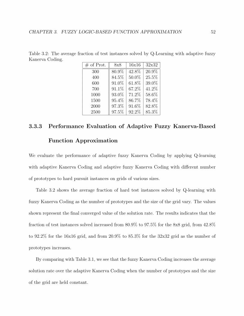
CHAPTER 3. FUZZY LOGIC-BASED FUNCTION APPROXIMATION 52
Table 3.2: The average fraction of test instances solved by Q-Learning with adaptive fuzzyKanerva Coding.
# of Prot. 8x8 16x16 32x32
300 80.9% 42.8% 20.9%400 84.5% 50.0% 25.5%600 91.0% 61.8% 39.0%700 91.1% 67.2% 41.2%1000 93.0% 71.2% 58.6%1500 95.4% 86.7% 78.4%2000 97.3% 91.6% 82.8%2500 97.5% 92.2% 85.3%
3.3.3 Performance Evaluation of Adaptive Fuzzy Kanerva-Based
Function Approximation
We evaluate the performance of adaptive fuzzy Kanerva Coding by applying Q-learning
with adaptive Kanerva Coding and adaptive fuzzy Kanerva Coding with different number
of prototypes to hard pursuit instances on grids of various sizes.
Table 3.2 shows the average fraction of hard test instances solved by Q-learning with
fuzzy Kanerva Coding as the number of prototypes and the size of the grid vary. The values
shown represent the final converged value of the solution rate. The results indicates that the
fraction of test instances solved increased from 80.9% to 97.5% for the 8x8 grid, from 42.8%
to 92.2% for the 16x16 grid, and from 20.9% to 85.3% for the 32x32 grid as the number of
prototypes increases.
By comparing with Table 3.1, we see that the fuzzy Kanerva Coding increases the average
solution rate over the adaptive Kanerva Coding when the number of prototypes and the size
of the grid are held constant.

CHAPTER 3. FUZZY LOGIC-BASED FUNCTION APPROXIMATION 53
!"##$%!"##$%
!"##$%
&'()$%
&'()$%
&'()$%
*%
*$+%
*$,%
*$-%
*$.%
*$/%
*$0%
*$1%
*$2%
*$3%
+%
+% ,% -%
!"#$%&#'()*+,
)-'.%/#'
0$12'(13#'
242% +04+0% -,4-,%
0.00
0.10
0.20
0.30
0.40
0.50
0.60
0.70
0.80
0.90
1.00
0 200 400 600 800 1000 1200 1400 1600 1800 2000
Avera
ge s
olu
tio
n r
ate
Epoch
(1) 8X 8 Grid, Fuzzy
(2) 8X 8 Grid, Adaptive
(3) 16X16 Grid, Fuzzy
(4) 16X16 Grid, Adaptive
(5) 32X32 Grid, Fuzzy
(6) 32X32 Grid, Adaptive,
!"#$!%#$
!&#$!'#$
!(#$
!)#$
Figure 3.7: Average solution rate for adaptive fuzzy Kanerva Coding with 2000 prototypes.
Figure 3.7 shows the average fraction of test instances solved when adaptive Kanerva and
adaptive fuzzy Kanerva-based function approximation are applied to our instances as the
number of prototypes varies. The results show that with 2000 prototypes, using the fuzzy
algorithm increases the fraction of the test instances solved over the adaptive algorithm from
83.4% to 91.6% in the grid of 16x16 and from 67.9% to 82.8% in the grid of 32x32. These
results indicates that the fuzzy algorithm increases the fraction of the test instances solved
over the adaptive Kanerva algorithm.

CHAPTER 3. FUZZY LOGIC-BASED FUNCTION APPROXIMATION 54
3.4 Prototype Tuning
While fuzzy Kanerva Coding can give good results for our instances, the quality of the results
is often unstable. That is, the average fraction of test instances solved by the fuzzy approach
may be low. An explanation for these results can be found by considering the similarity
of membership vectors across state-action pairs. Intuitively, the similarity of membership
vectors of state-action pairs is equivalent to the prototype collisions observed with traditional
Kanerva Coding. In both cases, it may reduce the quality of the results.
3.4.1 Experimental Evaluation: Similarity Analysis of Member-
ship Vectors
Figure 3.8(a) shows the average membership grade of each prototype with respect to all other
prototypes on a sample run. The prototypes are ordered by decreasing average membership
grade. The results show that prototypes fall into three general regions. On the left, the pro-
totypes have a higher average membership grade, corresponding to prototypes that are closer
on average to other prototypes. On the right, prototypes have a lower average membership
grade, corresponding to prototypes that are on average farther from other prototypes. The
prototypes on the left are in a region of the state-action space where the distribution of
prototypes is more dense, and prototypes on the right are in a region where the distribution
of prototypes is more sparse. This variation in the distribution of the prototypes causes the
receptive fields to be unevenly distributed across the state-action space.
State-action pairs in the dense region of the space are near to more prototypes and
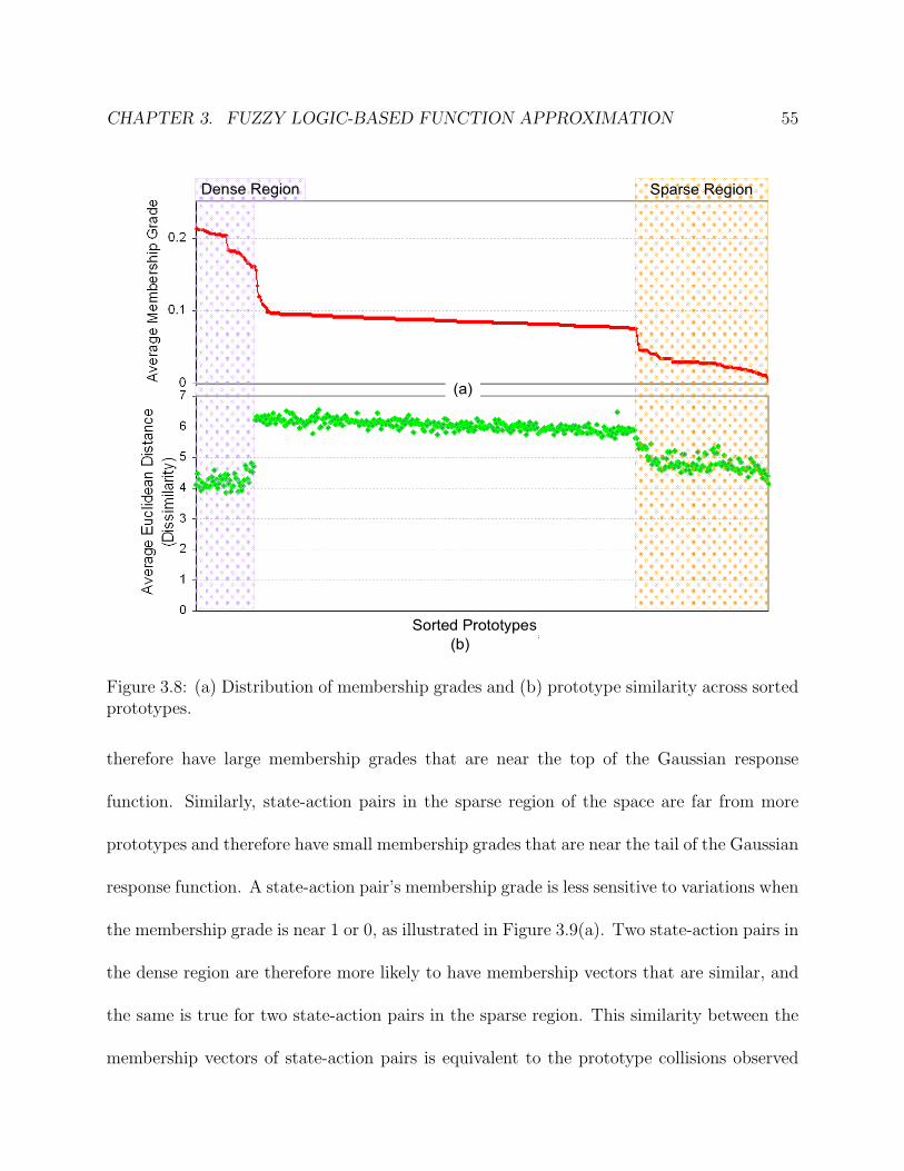
CHAPTER 3. FUZZY LOGIC-BASED FUNCTION APPROXIMATION 55
Figure 3.8: (a) Distribution of membership grades and (b) prototype similarity across sortedprototypes.
therefore have large membership grades that are near the top of the Gaussian response
function. Similarly, state-action pairs in the sparse region of the space are far from more
prototypes and therefore have small membership grades that are near the tail of the Gaussian
response function. A state-action pair’s membership grade is less sensitive to variations when
the membership grade is near 1 or 0, as illustrated in Figure 3.9(a). Two state-action pairs in
the dense region are therefore more likely to have membership vectors that are similar, and
the same is true for two state-action pairs in the sparse region. This similarity between the
membership vectors of state-action pairs is equivalent to the prototype collisions observed

CHAPTER 3. FUZZY LOGIC-BASED FUNCTION APPROXIMATION 56
A prototype’s membership
function
(a) Before prototype tuning.
A prototype’s
membership function
(b) After prototype tuning.
Figure 3.9: Illustration of the similarity of membership vectors across sparse and denseprototype regions.
with traditional Kanerva Coding, and may have a similar negative effect on the quality of
the results.
Figure 3.9(b) illustrates how the similarity between prototypes can vary across the state-
action space. The graph shows the average Euclidean distance between each prototype and
every other prototype. Prototypes in the dense and sparse regions have a smaller average
Euclidean distance, indicating that they are more similar to one another.

CHAPTER 3. FUZZY LOGIC-BASED FUNCTION APPROXIMATION 57
3.4.2 Tuning Mechanism
We can reduce the effect of similar membership vectors by adjusting the variance of the
Gaussian response function used to compute membership grades. The variance is decreased
in the dense region which narrows the Gaussian response function, and the variance is in-
creased in the sparse region which broadens the Gaussian response function. This prototype
tuning increases the sensitivity of state-action pairs’ membership vectors to variations in the
state-action space in these regions, as shown in Figure 3.9(b). We use Maximum Likelihood
Estimation to compute an estimate σ̂2i of the variance of a prototype’s membership func-
tion. Given a prototype i, we let dij be the bit difference between prototype pi and all other
prototypes pj, where j 6= i, and d̄i the sample mean of dij. The estimate of σ̂2i is
σ̂2i =
n∑j=1
(dij − d̄i)2/n,
where n is the number of prototypes.
3.4.3 Performance Evaluation of Tuning Mechanism
We evaluate our implementation of adaptive fuzzy Kanerva Coding with prototype tuning
by using it to solve pursuit instances on a grid of size 32x32. As a comparison, the adaptive
fuzzy and adaptive approaches are also implemented to solve the same instances.
Figure 3.10 shows the average fraction of test instances solved by adaptive fuzzy Kanerva
Coding with prototype tuning. We can see that using prototype tuning increases the fraction
of the test instances solved over the adaptive fuzzy algorithm and the adaptive algorithm.
For example, with 2000 prototypes, using prototype tuning increases the fraction of the test
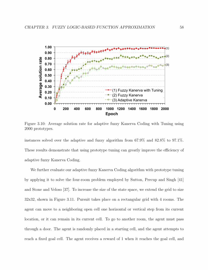
CHAPTER 3. FUZZY LOGIC-BASED FUNCTION APPROXIMATION 58
0.00 0.10 0.20 0.30 0.40 0.50 0.60 0.70 0.80 0.90 1.00
0 200 400 600 800 1000 1200 1400 1600 1800 2000
Aver
age
solu
tion
rate
Epoch
(1) Fuzzy Kanerva with Tuning (2) Fuzzy Kanerva (3) Adaptive Kanerva
(1)
(2)
(3)
Figure 3.10: Average solution rate for adaptive fuzzy Kanerva Coding with Tuning using2000 prototypes.
instances solved over the adaptive and fuzzy algorithm from 67.9% and 82.8% to 97.1%.
These results demonstrate that using prototype tuning can greatly improve the efficiency of
adaptive fuzzy Kanerva Coding.
We further evaluate our adaptive fuzzy Kanerva Coding algorithm with prototype tuning
by applying it to solve the four-room problem employed by Sutton, Precup and Singh [41]
and Stone and Veloso [37]. To increase the size of the state space, we extend the grid to size
32x32, shown in Figure 3.11. Pursuit takes place on a rectangular grid with 4 rooms. The
agent can move to a neighboring open cell one horizontal or vertical step from its current
location, or it can remain in its current cell. To go to another room, the agent must pass
through a door. The agent is randomly placed in a starting cell, and the agent attempts to
reach a fixed goal cell. The agent receives a reward of 1 when it reaches the goal cell, and

CHAPTER 3. FUZZY LOGIC-BASED FUNCTION APPROXIMATION 59
Figure 3.11: The four-room gridworld
receives a reward of 0 in every other cell.
Figure 3.12 compares the average fraction of test instances solved by adaptive fuzzy
Kanerva Coding with prototype tuning to solve the instances of the four-room problem. The
results show that using adaptive fuzzy Kanerva Coding with prototype tuning increases the
fraction of the test instances solved over using adaptive and adaptive fuzzy approaches. For
example, using adaptive fuzzy Kanerva Coding with prototype tuning with 2000 prototypes
increases the fraction of the test instances solved over using adaptive and adaptive fuzzy
approaches from 58.4% and 78.9% to 94.9%. These results again demonstrate that using
adaptive fuzzy Kanerva Coding with prototype tuning can greatly improve the quality of

CHAPTER 3. FUZZY LOGIC-BASED FUNCTION APPROXIMATION 60
0.00 0.10 0.20 0.30 0.40 0.50 0.60 0.70 0.80 0.90 1.00
0 200 400 600 800 1000 1200 1400 1600 1800 2000
Aver
age
solu
tion
rate
Epoch
(1) Fuzzy Kanerva with Tuning (2) Fuzzy Kanerva (3) Adaptive Kanerva
(1)
(2)
(3)
Figure 3.12: Average solution rate for adaptive Fuzzy Kanerva Coding with Tuning in thefour-room gridworld of size 32x32.
the results obtained.
3.5 Summary
In this chapter, we evaluated a class of hard pursuit instances of the predator-prey prob-
lem and argued that this poor performance is caused by frequent prototype collisions. We
also showed that dynamic prototype allocation and adaptation can partially reduce these
collisions and give better results. However the collision rate remained quite high and the
performance was still poor for large-scale instances. It was therefore necessary to consider a
more effective approach for eliminating the collision rate as the dimension of the state-action
space increases.
Our new fuzzy approach to Kanerva-based function approximation uses a fine-grained
CHAPTER 3. FUZZY LOGIC-BASED FUNCTION APPROXIMATION 61
fuzzy membership grade to describe a state-action pair’s adjacency with respect to each
prototype. This approach, coupled with adaptive prototype allocation, allows the solver to
distinguish membership vectors and reduce the collision rate. Our adaptive fuzzy Kanerva
approach gives better performance than the pure adaptive Kanerva algorithm. We then
showed that prototype density varies widely across the state-action space, causing prototypes’
receptive fields to be unevenly distributed across the state-action space. State-action pairs
in dense or sparse regions of the space are more likely to have similar membership vectors
which limits the performance of a reinforcement learner based on Kanerva Coding. Our
fuzzy framework for Kanerva-based function approximation allows us to tune the prototype
receptive fields to balance the effects of prototype density variations, further increasing the
fraction of test instances solved using this approach. We conclude that adaptive fuzzy
Kanerva Coding with prototype tuning can significantly improve a reinforcement learner’s
ability to solve large-scale high dimension problems.
Chapter 4
Rough Sets-based Function
Approximation
Fuzzy Kanerva-based function approximation can significantly improve the efficiency of
function approximation within reinforcement learners. As we described in Chapter 3, this
approach distinguishes frequently-visited state-actions pairs by using a fine-grained fuzzy
membership grade to describe a state-action pair’s adjacency with respect to each proto-
type. In this way, the fuzzy approach completely eliminates prototype collisions. We have
shown that this approach gives a function approximation architecture that outperforms other
approaches.
However, our experimental results show that this approach often gives poor performance
when solving hard large-scale instances and shows unstable behavior when changing the
62
CHAPTER 4. ROUGH SETS-BASED FUNCTION APPROXIMATION 63
number of prototypes. We therefore extend our work to improve our algorithm. In this
chapter, we show that choosing an optimal number of prototypes can improve the efficiency
of function approximation. We propose to use the theory of rough sets to measure how
closely an approximate value function is approximating the true value function and determine
whether more prototypes are required. Finally, we describe a rough sets-based approach to
selecting prototypes for a Kanerva-based reinforcement learner.
4.1 Experimental Evaluation: Effect of Varying Num-
ber of Prototypes
The efficiency of Kanerva-based function approximation depends largely on the number
of prototypes. It is clear that the efficiency of our function approximator decreases as the
number of prototypes decreases. We therefore investigate the performance of a reinforcement
learner with adaptive Kanerva Coding as the number of prototypes decreases.
We evaluate the effect of varying the number of prototypes by applying Q-learning with
adaptive Kanerva Coding to the class of predator-prey pursuit instances. The state-action
pairs are represented as prototype vectors and all prototypes are selected randomly. Prob-
abilistic prototype deletion with prototype splitting is used as feature optimization. The
number of prototypes varies from 300 to 2500. The size of the grid varies from 8x8 to 32x32.
Table 4.2 shows the average fraction of test instances solved by Q-learning with adaptive
Kanerva Coding as the number of prototypes and the size of the grid vary. The values shown
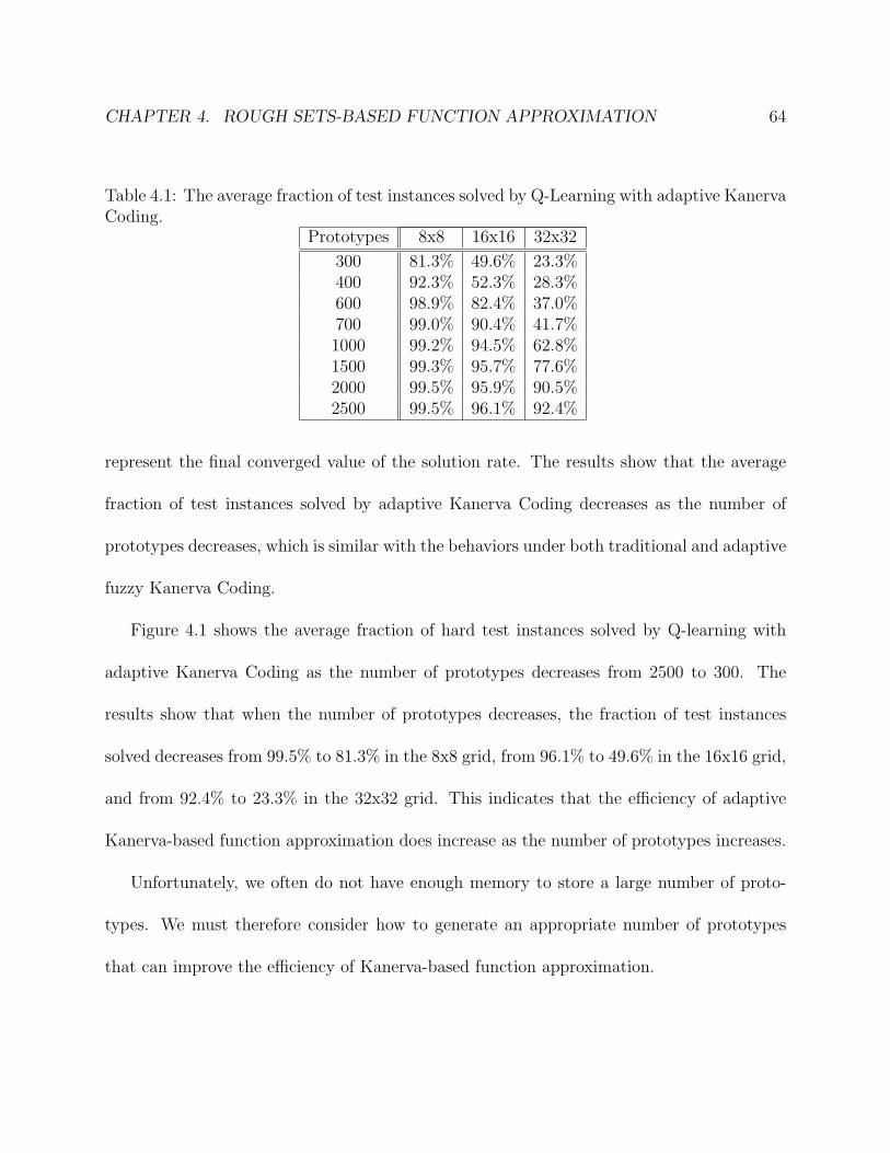
CHAPTER 4. ROUGH SETS-BASED FUNCTION APPROXIMATION 64
Table 4.1: The average fraction of test instances solved by Q-Learning with adaptive KanervaCoding.
Prototypes 8x8 16x16 32x32
300 81.3% 49.6% 23.3%400 92.3% 52.3% 28.3%600 98.9% 82.4% 37.0%700 99.0% 90.4% 41.7%1000 99.2% 94.5% 62.8%1500 99.3% 95.7% 77.6%2000 99.5% 95.9% 90.5%2500 99.5% 96.1% 92.4%
represent the final converged value of the solution rate. The results show that the average
fraction of test instances solved by adaptive Kanerva Coding decreases as the number of
prototypes decreases, which is similar with the behaviors under both traditional and adaptive
fuzzy Kanerva Coding.
Figure 4.1 shows the average fraction of hard test instances solved by Q-learning with
adaptive Kanerva Coding as the number of prototypes decreases from 2500 to 300. The
results show that when the number of prototypes decreases, the fraction of test instances
solved decreases from 99.5% to 81.3% in the 8x8 grid, from 96.1% to 49.6% in the 16x16 grid,
and from 92.4% to 23.3% in the 32x32 grid. This indicates that the efficiency of adaptive
Kanerva-based function approximation does increase as the number of prototypes increases.
Unfortunately, we often do not have enough memory to store a large number of proto-
types. We must therefore consider how to generate an appropriate number of prototypes
that can improve the efficiency of Kanerva-based function approximation.

CHAPTER 4. ROUGH SETS-BASED FUNCTION APPROXIMATION 65
0%
20%
40%
60%
80%
100%
300 400 600 700 1000 1500 2000 2500
Aver
age
Solu
tion
Rat
e
Number of Prototypes
(1) 8x 8 Grid (2) 16x16 Grid (3) 32x32 Grid
(1)(2)(3)
Figure 4.1: The fraction of hard test instances solved by Q-learning with adaptive KanervaCoding as the number of prototypes decreases.
4.2 Rough Sets and Kanerva Coding
In traditional Kanerva Coding, a set of state-action pairs is selected from the state-action
space as prototypes. We assume that P is the set of prototypes, Λ is the set of all possible
state-action pairs in the state-action space, and SA is the set of state-action pairs encountered
by the solver. For Kanerva-based function approximation, P ⊆ Λ and SA ⊆ Λ. Our goal is
to represent a set of observed state-action pairs SA using a set of prototypes P . That is, given
an arbitrary set of state-action pairs SA, we wish to express the set using an approximate
set induced by prototype set P .
Assume that the function fp(sa) represents the adjacency between prototype p and state-
action pair sa. That is, if sa is adjacent to p, fp(sa) is equal to 1, otherwise it equals 0.

CHAPTER 4. ROUGH SETS-BASED FUNCTION APPROXIMATION 66
Table 4.2: Sample of adjacency between state-action pairs and prototypes.p1 p2 p3 p4 p5 p6
sa1 0 0 0 0 1 1sa2 1 0 0 1 1 1sa3 1 1 0 0 0 1sa4 0 1 0 0 1 1sa5 0 1 0 0 1 1sa6 1 1 0 1 0 1sa7 0 0 0 0 0 1sa8 0 0 0 0 0 1sa9 0 1 1 1 1 1sa10 0 0 0 0 0 1
The set of adjacency values for a state-action pair with respect to all prototypes is referred
as the state-action pair’s prototype vector. On the basis of prototype set P , we define an
indiscernibility relation, denoted IND(P ):
IND(P ) = {(sa1, sa2) ∈ Λ2|∀p ∈ P, fp(sa1) = fp(sa2)}.
where p is a prototype and sa1 and sa2 are two state-action pairs, that is, sa1 ∈ SA,
sa2 ∈ SA. If any two state-action pairs sa1 and sa2 in the set SA are indiscernible by the
prototypes in P , there is an associated indiscernibility relation between sa1 and sa2. The
set of state-action pairs with the same indiscernibility relation is defined as an equivalence
class, and the ith such equivalence class is denoted EPi . The set of prototypes P therefore
partitions the set SA into a collection of equivalence classes, denoted {EP}.
For example, assume ten state-action pairs, (sa1, sa2, sa3, ..., sa10), are encountered
by a solver, and we have six prototypes, (p1, p2, p3, ..., p6). We attempt to express each
state-action pair using prototypes. Table 4.2 shows a sample of the adjacencies between
state-action pairs and prototypes. When the prototypes are considered, we can induce the
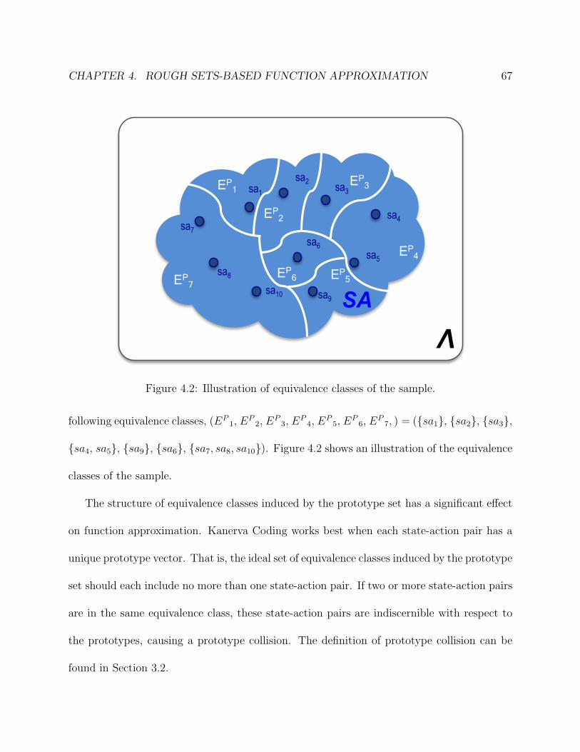
CHAPTER 4. ROUGH SETS-BASED FUNCTION APPROXIMATION 67
ΛSA
sa1 sa2 sa3
sa4
sa5 sa6
sa9
sa7
sa8 sa10
EP1
EP2
EP3
EP4
EP5 EP
6 EP7
Figure 4.2: Illustration of equivalence classes of the sample.
following equivalence classes, (EP1, E
P2, E
P3, E
P4, E
P5, E
P6, E
P7, ) = ({sa1}, {sa2}, {sa3},
{sa4, sa5}, {sa9}, {sa6}, {sa7, sa8, sa10}). Figure 4.2 shows an illustration of the equivalence
classes of the sample.
The structure of equivalence classes induced by the prototype set has a significant effect
on function approximation. Kanerva Coding works best when each state-action pair has a
unique prototype vector. That is, the ideal set of equivalence classes induced by the prototype
set should each include no more than one state-action pair. If two or more state-action pairs
are in the same equivalence class, these state-action pairs are indiscernible with respect to
the prototypes, causing a prototype collision. The definition of prototype collision can be
found in Section 3.2.

CHAPTER 4. ROUGH SETS-BASED FUNCTION APPROXIMATION 68
Given a set of prototypes, one or more prototypes may not affect the structure of the
induced equivalence classes, and therefore do not help differentiate state-action pairs. These
prototypes can be replaced with prototypes that are more useful. To do this, we use a
reduct of the prototype set. A reduct is a subset of prototypes R ⊆ P such that (1)
{ER} = {EP}, that is, the equivalence classes induced by reduced prototype set R are the
same as the equivalence classes induced by original prototype set P; and (2) R is minimal,
that is {E(R−{p})} 6= {EP} for any prototype p ∈ R. Thus, no prototype can be removed
from reduced prototype set R without changing the equivalence classes EP .
In the above example, the subset (p2, p4, p5) is a reduct of the original prototype set
P . This can be shown easily because (1) the equivalence classes induced by (p2, p4, p5) are
the same as the equivalence class structure induced by the original prototype set P; and (2)
eliminating any of these prototypes alters the equivalence class structure that is induced.
Replacing a set of prototypes with its reduct eliminates unnecessary prototypes. Adaptive
prototype optimization can also eliminate unnecessary prototypes by deleting rarely-visited
prototypes, but that approach cannot eliminate prototypes that are heavily-visited but un-
necessary, such as prototype p6 in the above example. Note that all state-action pairs are
adjacent to this prototype, but deleting it does not change the structure of the equivalence
classes.
We evaluate the structure of equivalence classes and the reduct of prototypes in traditional
Kanerva Coding and adaptive Kanerva Coding. We apply traditional Kanerva and adaptive
Kanerva with 2000 prototypes to sample predator-prey instances of varying sizes.
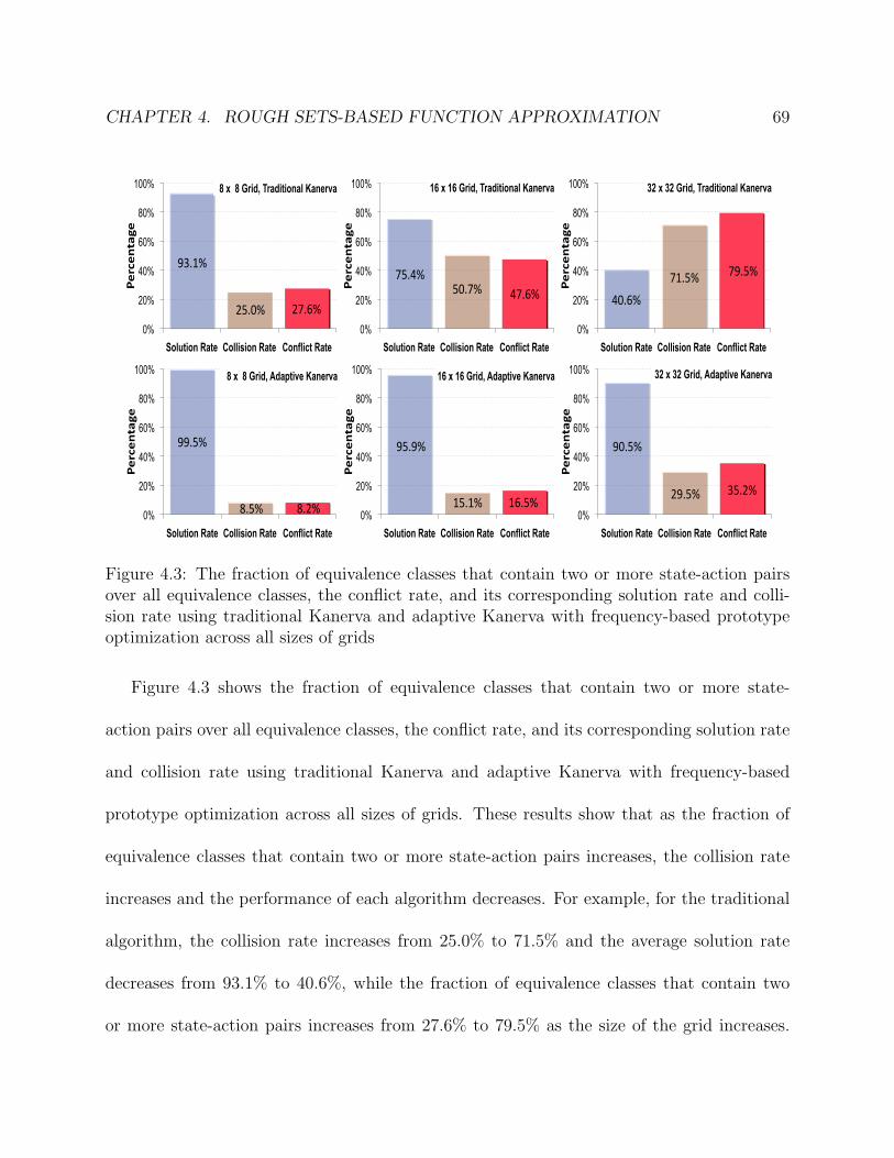
CHAPTER 4. ROUGH SETS-BASED FUNCTION APPROXIMATION 69
93.1%
25.0% 27.6%0%
20%
40%
60%
80%
100%
Solution Rate Collision Rate Conflict Rate
Percentage
8 x 8 Grid, Traditional Kanerva
75.4%50.7% 47.6%
0%
20%
40%
60%
80%
100%
Solution Rate Collision Rate Conflict Rate Percentage
16 x 16 Grid, Traditional Kanerva
40.6%
71.5% 79.5%
0%
20%
40%
60%
80%
100%
Solution Rate Collision Rate Conflict Rate
Percentage
32 x 32 Grid, Traditional Kanerva
99.5%
8.5% 8.2%0%
20%
40%
60%
80%
100%
Solution Rate Collision Rate Conflict Rate
Percentage
8 x 8 Grid, Adaptive Kanerva
95.9%
15.1% 16.5%0%
20%
40%
60%
80%
100%
Solution Rate Collision Rate Conflict Rate
Percentage
16 x 16 Grid, Adaptive Kanerva
90.5%
29.5% 35.2%
0%
20%
40%
60%
80%
100%
Solution Rate Collision Rate Conflict Rate
Percentage
32 x 32 Grid, Adaptive Kanerva
Figure 4.3: The fraction of equivalence classes that contain two or more state-action pairsover all equivalence classes, the conflict rate, and its corresponding solution rate and colli-sion rate using traditional Kanerva and adaptive Kanerva with frequency-based prototypeoptimization across all sizes of grids
Figure 4.3 shows the fraction of equivalence classes that contain two or more state-
action pairs over all equivalence classes, the conflict rate, and its corresponding solution rate
and collision rate using traditional Kanerva and adaptive Kanerva with frequency-based
prototype optimization across all sizes of grids. These results show that as the fraction of
equivalence classes that contain two or more state-action pairs increases, the collision rate
increases and the performance of each algorithm decreases. For example, for the traditional
algorithm, the collision rate increases from 25.0% to 71.5% and the average solution rate
decreases from 93.1% to 40.6%, while the fraction of equivalence classes that contain two
or more state-action pairs increases from 27.6% to 79.5% as the size of the grid increases.

CHAPTER 4. ROUGH SETS-BASED FUNCTION APPROXIMATION 70
For the adaptive algorithm, the collision rate increases from 8.5% to 29.5% and the average
solution rate decreases from 99.5% to 90.5%, while the fraction of equivalence classes that
contain two or more state-action pairs increases from 8.2% to 35.2% as the size of the grid
increases.
The results also demonstrate that the improved performance of the adaptive Kanerva
algorithm over the traditional algorithm is due to the reduction of the fraction of equivalence
classes that contain two or more state-action pairs. For example, the adaptive algorithm
reduces the fraction of equivalence classes that contain two or more state-action pairs from
79.5% to 35.2% while the average solution rate for the adaptive algorithm increases from
40.6% to 90.5% for a grid size of 32x32.
Figure 4.4 shows the fraction of prototypes remaining after performing a prototype reduct
using traditional and optimized Kanerva-based function approximation with 2000 proto-
types. The original and final number of prototypes is shown on each bar. The results
indicate that the structure of the equivalence classes can be maintained using fewer proto-
types. For example, the equivalence classes induced by 1821 prototypes for the adaptive
algorithm using frequency-based prototype optimization are same as the equivalence classes
induced by 2000 prototypes for a grid size of 32.
4.3 Rough Sets-based Kanerva Coding
A more reliable approach to prototype optimization for function approximation is to apply
rough sets theory to reformulate Kanerva-based function approximation. Instead of using

CHAPTER 4. ROUGH SETS-BASED FUNCTION APPROXIMATION 71
0% 10% 20% 30% 40% 50% 60% 70% 80% 90%
100%
Trad. Adap. Trad. Adap. Trad. Adap.
% of
origi
nal p
roto
type i
n red
uct
Grid size 8X8 16X16 32X32
821
/ 200
0
943
/ 200
0
1368
/ 20
00
1476
/ 20
00
1753
/ 20
00
1821
/ 20
00
Figure 4.4: The fraction of prototypes remaining after performing a prototype reduct usingtraditional and optimized Kanerva-based function approximation with 2000 prototypes. Theoriginal and final number of prototypes is shown on each bar.
visit frequencies for frequency-based prototype optimization, we focus on the structure of
equivalence classes induced by the set of prototypes, a key indicator of the efficiency of
function approximation. When the fraction of equivalence classes that contain two or more
state-action pairs increases, the performance of a reinforcement learner based on Kanerva
coding decreases. Since a prototype reduct maintains the equivalence class structure, pro-
totype deletion can be conducted by replacing the set of prototypes with a reduct of the
original prototype set. Since prototype collisions occur only when two state-action pairs are
in a same equivalence class, prototype generation should reduce the fraction of equivalence
classes that contain two or more state-action pairs.

CHAPTER 4. ROUGH SETS-BASED FUNCTION APPROXIMATION 72
4.3.1 Prototype Deletion and Generation
In rough sets-based Kanerva coding, if the structure of equivalence classes remains un-
changed, the efficiency of function approximation is also unchanged. Replacing a set of
prototypes with its reduct clearly eliminates unnecessary prototypes. We therefore imple-
ment prototype deletion by finding a reduct R of original prototype set P . We refer to this
approach as reduct-based prototype deletion.
Note that a reduct of prototype set is not necessarily unique, and there may be many
subsets of prototypes which preserve the equivalence-class structure. The following algorithm
finds a reduct of original prototype set. We consider each prototype in P one by one. For
prototype p ∈ P , if the set of equivalence classes {EP−{p}} induced by P − {p} is not identical
to the equivalence classes {EP} induced by P , that is, {EP−{p}} 6= {EP}, then p is in a reduct
R of original prototype set P , p ∈ R; otherwise, p is not in the reduct R, p /∈ R. We then
delete p from prototype set P and consider the next prototype. The final set R is a reduct
of original prototype set P . We find a series of random reducts of the original prototype set,
then select a reduct with the fewest elements to be the replacement of original prototype
set. Reduct-based prototype optimization makes only a few passes through the prototypes
and is not time-consuming. With n state-action pairs and p prototypes, the complexity is
O(n ∗ p2). Once a prototype is deleted, the θ-value of this prototype is accumulated to the
nearest prototypes.
In rough sets-based Kanerva coding, if the number of equivalence classes that contain
only one state-action pair increases, prototype collisions are less likely and the efficiency of

CHAPTER 4. ROUGH SETS-BASED FUNCTION APPROXIMATION 73
function approximation increases. An equivalence class that contains two or more state-
action pairs is likely to be split up by adding a new prototype equal to one of those state-
action pairs. We therefore implement prototype generation by adding new prototypes that
split equivalence classes with two or more state-action pairs. We refer to this approach as
equivalence class-based prototype generation.
For an arbitrary equivalence class that contains n > 1 state-ation pairs, we randomly
select dlog(n)e state-ation pairs to be new prototypes. Note that this value is the smallest
number of prototypes needed to distinguish all state-action pairs in an equivalence class that
contains n elements. This algorithm does not guarantee that each equivalence class will be
split into new classes that contain exactly one state-action pair. For example, this approach
cannot split an equivalence class with two neighboring state-action pairs. In this case, we
add such a new prototype that is a neighbor of one state-action pair, but not a neighbor of
the other.
4.3.2 Rough Sets-based Kanerva Coding Algorithm
Algorithm 2 describes our algorithm for implementing Q-learning with adaptive Kanerva
coding using rough sets-based prototype optimization. The algorithm begins by initializing
parameters, and repeatedly executes Q-learning with adaptive Kanerva Coding. Prototypes
are adaptively updated periodically. In each update period, the encountered state-action
pairs are recorded. To update prototypes, the algorithm first determines the structure of
the equivalence classes of the set of encountered state-action pairs with respect to original

CHAPTER 4. ROUGH SETS-BASED FUNCTION APPROXIMATION 74
Algorithm 2 Pseudo code of Q-learning with rough sets-based Kanerva Coding
Main()
choose a set of prototypes ~p and initial their ~θ value;repeat
Generate initial state-action pair s from initial state ς and action aQ-with-Kanerva(s, a, ~p, ~θ)
Update-prototypes(~p, ~θ)until all episodes are traversed
Q-with-Kanerva(s, a, ~p, ~θ)repeat
Take action a, observe reward r, get next state ς’Q(sa) =
∑ ~θ;for all actions a* under new state ς’ do
Generate the state-action pair sa’ from state ς’ and action a*Q(sa′) =
∑ ~θ;end forδ = r + γ ∗maxQ(s′)−Q(sa)
∆~θ = α ∗ δ~θ = ~θ + ∆~θif random probability ≤ ε then
for all actions a* under current state s doQ̂(sa) =
∑ ~θ;a = argmaxaQ(sa)
end forelsea = random action
end ifuntil s is terminal
Update-prototypes(~p, ~θ)
Prototype-reduct-based-Deletion(~p, ~θ);
Equivalent-class-based-Generation(~p, ~θ).

CHAPTER 4. ROUGH SETS-BASED FUNCTION APPROXIMATION 75
Prototype-reduct-based-Deletion(~p, ~θ)−−→E(~p) = equivalence classes induced by ~p~preduct = ~pfor i = 0 to 10 do~ptmp = ~prepeat~̂p = ~ptmp − p−−→E(~̂p) = equivalence classes induced by ~̂p
if−−→E(~̂p) =
−−→E(~p) then
~ptmp = ~̂pend if
until all prototypes p ∈ ~ptmp are traversed.if |~preduct| > |~ptmp| then~preduct = ~ptmp
end ifend for
Equivalent-class-based-Generation(~p, ~θ)repeatn = size(E(~p))if n > 1 then
if (n = 2) and (two state-action pairs sa1 and sa2 are neighbor) then~p = ~p
⋃{p|p = a neighbor of sa1, but not a neighbor of sa2}
elserepeat
randomly select a state-action pair sa~p = ~p
⋃{sa}
until dlog(n)e new prototypes are generated.end if
end if
until all equivalence classes E(~p) ∈−−→E(~p) are traversed.

CHAPTER 4. ROUGH SETS-BASED FUNCTION APPROXIMATION 76
prototypes. Unnecessary prototypes are then deleted by replacing the original prototype set
with a reduct with the fewest elements among ten randomly-generated reducts. In order to
split large equivalence classes, new prototypes are randomly selected from these equivalence
classes. For the equivalence classes with two neighboring state-action pairs, a new prototype
is a neighbor of one state-action pair, but not a neighbor of the other. The optimized
prototype set is constructed by adding newly generated prototypes to the reduct of original
prototype set.
4.3.3 Performance Evaluation of Rough Sets-based Kanerva Cod-
ing
We evaluate the performance of rough sets-based Kanerva coding by using it to solve pursuit
instances on grids of varying sizes. As a comparison, traditional Kanerva coding and adaptive
Kanerva coding with different number of prototypes are also applied to the same instances.
Traditional Kanerva coding follows Sutton [38]. Kanerva coding with adaptive prototype
optimization is implemented using prototype deletion and prototype splitting. A detailed
description of prototype deletion and splitting can be found in Section 3.3. When rough
sets-based Kanerva coding is implemented during a learning process, we also observe the
change in the number of prototypes and the fraction of equivalence classes that contain only
one state-action pair.
Figure 4.5 shows the average fraction of test instances solved when traditional Kanerva,
adaptive Kanerva, and rough sets-based Kanerva are applied to our instances with grids of

CHAPTER 4. ROUGH SETS-BASED FUNCTION APPROXIMATION 77
0.00
0.10
0.20
0.30
0.40
0.50
0.60
0.70
0.80
0.90
1.00
0 200 400 600 800 1000 1200 1400 1600 1800 2000
Aver
age
solu
tion
rate
Epoch
Rough Set-based Optimization, 568 prototypes Frequence-based Optimization with 2000 Prototypes Frequence-based Optimization with 568 Prototypes No Optimization with 2000 Prototypes
(a)
0.00
0.10
0.20
0.30
0.40
0.50
0.60
0.70
0.80
0.90
1.00
0 200 400 600 800 1000 1200 1400 1600 1800 2000
Aver
age
solu
tion
rate
Epoch
Rough Set-based Optimization, 955 Prototypes Frequence-based Optimization with 2000 Prototypes Frequence-based Optimization with 955 Prototypes No Optimization with 2000 Prototypes
(b)
0.00
0.10
0.20
0.30
0.40
0.50
0.60
0.70
0.80
0.90
1.00
0 200 400 600 800 1000 1200 1400 1600 1800 2000
Aver
age
solu
tion
rate
Epoch
Rough Set-based Optimization, 1968 Prototypes Frequence-based Optimization with 2000 Prototypes Frequence-based Optimization with 1968 Prototypes No Optimization with 2000 Prototypes
(c)
Figure 4.5: Average solution rate for traditional Kanerva, adaptive Kanerva and rough sets-based Kanerva (a), in 8x8 grid; (b), in 16x16 grid; (c), in 32x32 grid.

CHAPTER 4. ROUGH SETS-BASED FUNCTION APPROXIMATION 78
Table 4.3: Percentage improved performance of rough sets-based Kanerva over adaptiveKanerva.
Size 4x4 8x8 16x16 32x32 64x64Gap 13.2% 11.8% 24.6% 11.7% 16.5%
size 8, 16 and 32. The results show that the rough sets-based algorithm increases the fraction
of test instances solved over adaptive Kanerva algorithm when using the same number of
prototypes. For example, after 2000 epochs, using the rough sets-based algorithm increases
the fraction of test instances solved over the adaptive algorithm from 87.6% to 99.4% in the
8x8 grid, from 73.4% to 98.0% in the 16x16 grid and from 81.1% to 92.8% in the 32x32
grid, respectively . The results when using grids of varying sizes indicate that rough sets-
based Kanerva coding uses fewer prototypes and achieves higher performance by adaptively
changing the number and allocation of prototypes.
Table 4.3 shows the percentage improved performance using rough sets-based Kanerva
over adaptive Kanerva across varying grid sizes. The results show that the improved per-
formance of the rough sets-based approach is consistently more than 10% better than the
adaptive approach with different grids of size. It indicates that our rough sets-based approach
can reliably improve a Kanerva-based reinforcement learner’s ability.
Figure 4.6 shows the effect of our rough sets-based Kanerva coding on the number of
prototypes and the corresponding change in the fraction of equivalence classes that contain
only one state-action pair in the grid of size 8, 16 and 32.. The results show that the
rough sets-based algorithm reduces the number of prototypes and increases the fraction of
equivalence classes with only one state-action pair. For example, after 2000 epochs, the rough

CHAPTER 4. ROUGH SETS-BASED FUNCTION APPROXIMATION 79
2000 Prototypes
568 Prototypes
0%
10%
20%
30%
40%
50%
60%
70%
80%
90%
100%
0
500
1000
1500
2000
2500
0 200 400 600 800 1000 1200 1400 1600 1800 2000
% o
f equ
ival
ence
cla
sses
that
con
tain
onl
y on
e st
ate-
actio
n pa
ir
Num
ber o
f pro
toty
pes
Epoch
(a)
2000 Prototypes
955 Prototypes
0%
10%
20%
30%
40%
50%
60%
70%
80%
90%
100%
0
500
1000
1500
2000
2500
0 200 400 600 800 1000 1200 1400 1600 1800 2000
% o
f equ
ival
ence
cla
sses
that
con
tain
onl
y on
e st
ate-
actio
n pa
ir
Num
ber o
f pro
toty
pes
Epoch
(b)
2000 Prototypes 1968 Prototypes
0%
10%
20%
30%
40%
50%
60%
70%
80%
90%
100%
0
500
1000
1500
2000
2500
0 200 400 600 800 1000 1200 1400 1600 1800 2000
% o
f equ
ival
ence
cla
sses
that
con
tain
onl
y on
e st
ate-
actio
n pa
ir
Num
ber o
f pro
toty
pes
Epoch
(c)
Figure 4.6: Effect of rough sets-based Kanerva on the number of prototypes and the fractionof equivalence classes (a), in 8x8 grid; (b), in 16x16 grid; (c), in 32x32 grid.
CHAPTER 4. ROUGH SETS-BASED FUNCTION APPROXIMATION 80
sets-based algorithm reduces the number of prototypes to 568, 955 and 1968 prototypes, and
increases the fraction of equivalence classes with one state-action pair to 99.5%, 99.8% and
94.9% in the grid of size 8, 16 and 32, respectively. These results also demonstrate that
rough sets-based Kanerva can adaptively explore the optimal number of prototypes and
dynamically allocate prototypes for optimal structure of equivalence classes in a particular
application.
4.4 Effect of Varying the Number of Initial Prototypes
The accuracy of Kanerva-based function approximation is sensitive to the number of pro-
totypes. In general, more prototypes are needed to approximate the state-action space for
more complex applications. On the other hand, the computational complexity of Kanerva
Coding also depends entirely on the number of prototypes, and larger sets of prototypes
can more accurately approximate more complex spaces. Neither traditional Kanerva nor
adaptive Kanerva can adaptively select the number of prototypes. Therefore, the number
of prototypes has a significant effect on the efficiency of traditional and adaptive Kanerva
coding. If the number of prototypes is too large relative to the number of state-action pairs,
the implementation of Kanerva coding is unnecessarily time-consuming. If the number of
prototypes is too small, even if the prototypes are well chosen, the approximate values will
not be similar to true values and the reinforcement learner will give poor results. Select-
ing the appropriate number of prototypes is difficult for traditional and adaptive Kanerva
coding, and in most known applications of these algorithms the number of prototypes is

CHAPTER 4. ROUGH SETS-BASED FUNCTION APPROXIMATION 81
2000 Prototypes
975 Prototypes
1500 Prototypes
1000 Prototypes
500 Prototypes
250 Prototypes
0 Prototype
922 Prototypes
0
500
1000
1500
2000
2500
0 200 400 600 800 1000 1200 1400 1600 1800 2000
Num
ber o
f pro
toty
pes
Epoch
Figure 4.7: Variation in the number of prototypes with different numbers of initial prototypeswith rough sets-based Kanerva in a 16x16 grid.
selected manually. However, for a particular application, the set of observed state-action
pairs is limited to a fixed subset of all possible state-action pairs. The number of prototypes
needed to distinguished this set of state-action pairs is also fixed.
We are interested in investigating the effect of different number of initial prototypes using
rough sets-based Kanerva coding. We use our rough sets-based algorithm with 0, 250, 500,
1000, 1500 or 2000 initial prototypes to solve pursuit instances in the 16 X 16 grid. Figure 4.7
shows the effect of our algorithm on the number of prototypes. The results show that the
number of prototypes tends to converge to a fixed number in the range from 922 to 975 after
2000 epochs. The results demonstrate that our rough sets-based Kanerva coding has the
ability to adaptively determine an effective number of prototypes during a learning process.

CHAPTER 4. ROUGH SETS-BASED FUNCTION APPROXIMATION 82
4.5 Summary
Kanerva Coding can be used to improve the performance of function approximation within
reinforcement learners. This approach often gives poor performance when applied to large-
scale systems. We evaluated a collection of pursuit instances of the predator-prey problem
and argued that the poor performance is caused by inappropriate selection of the prototypes,
including the number and allocation of these prototypes. We also showed that adaptive
Kanerva coding can give better results by dynamically allocating the prototypes. However
the number of prototypes remains hard to select and the performance was still poor because
of inappropriate number of prototypes. It was therefore necessary to consider a more effective
approach for adaptively selecting the number of prototypes.
Our new rough sets-based Kanerva-based function approximation uses rough sets theory
to reformulate prototype set and its implementation in Kanerva Coding. This approach uses
the structure of equivalent classes to explain how prototype collisions occur. Our algorithm
eliminates unnecessary prototypes by replacing the original prototype set with its reduct, and
reduces prototype collisions by splitting equivalence classes with two or more state-action
pairs. Our results indicate that rough sets-based Kanerva coding can adaptively select an
effective number of prototypes and greatly improve a Kanerva-based reinforcement learner’s
ability to solve large-scale problems.

Chapter 5
Real-world Application: Cognitive
Radio Network
5.1 Introduction
Radio frequency spectrum is a scarce resource. In many countries, the governmental agencies,
e.g. the Federal Communications Commission (FCC) in the United States, assign spectrum
bands to specific operators or devices to prevent them from being used by unlicensed users.
However, much of these assigned bands depend strongly on time and place, and often are
rarely used. Recent studies have demonstrated that much of the radio frequency spectrum
is inefficiently utilized [35, 5]. To address this issue, the FCC has recently recently begun to
allow unlicensed users to utilize licensed bands whenever it would not cause any interference
83

CHAPTER 5. REAL-WORLD APPLICATION: COGNITIVE RADIO NETWORK 84
[1]. Therefore, dynamic spectrum management techniques are needed to improve the effi-
ciency of spectrum utilization [5, 18, 29]. The development of these techniques motivates a
novel research area of cognitive radio (CR) networks.
The key idea of CR networks is that the unlicensed devices (also called cognitive radio
users) detect vacant spectrum and utilize it without harmful interference with licensed de-
vices (also known as primary users). This approach requires that CR networks have the
ability to sense spectrum holes and capture the best transmission parameters to meet the
quality-of-service (QoS) requirements. However, in a real-world ad-hoc networks, dynamic
network topology and varying spectrum availability on different time slots and locations pose
a critical challenge for CR networks.
Recent studies have shown that applying theoretical research on multi-agent reinforce-
ment learning to spectrum management in CR network is a feasible approach for meeting
the challenge [50]. Since a CR network must have sufficient computational intelligence to
choose its appropriate transmission parameters based on external network environment, it
must be capable of learning from its historical experience, and adapting its behavior to the
current context. This approach works well to solve small topology networks. However, it
often gives poor performance when applied to large-scale networks. These networks typi-
cally have a very large number of unlicensed and licensed users, and a wide range of possible
transmission parameters. The experimental results have shown that the performance of CR
networks decreases sharply as the size of network increases [50]. There is therefore a need for
algorithms to apply function approximation techniques to scale up reinforcement learning
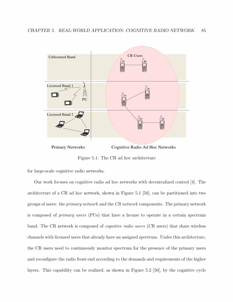
CHAPTER 5. REAL-WORLD APPLICATION: COGNITIVE RADIO NETWORK 85
Cognitive Radio Ad Hoc Networks
PU
Licensed Band 1
Unlicensed Band
Licensed Band 2
CR Users
Primary Networks
Figure 5.1: The CR ad hoc architecture
for large-scale cognitive radio networks.
Our work focuses on cognitive radio ad hoc networks with decentralized control [4]. The
architecture of a CR ad hoc network, shown in Figure 5.1 [50], can be partitioned into two
groups of users: the primary network and the CR network components. The primary network
is composed of primary users (PUs) that have a license to operate in a certain spectrum
band. The CR network is composed of cognitive radio users (CR users) that share wireless
channels with licensed users that already have an assigned spectrum. Under this architecture,
the CR users need to continuously monitor spectrum for the presence of the primary users
and reconfigure the radio front-end according to the demands and requirements of the higher
layers. This capability can be realized, as shown in Figure 5.2 [50], by the cognitive cycle

CHAPTER 5. REAL-WORLD APPLICATION: COGNITIVE RADIO NETWORK 86
Spectrum
Decision
Spectrum
Sharing
Radio
EnvironmentTransmitted
Signal
Spectrum
Characterization
PU Detection
RF Stimuli
Spectrum Hole
Decision Request
Spectrum
Channel Capacity
Mobility
Spectrum
Sensing
Figure 5.2: The cognitive radio cycle for the CR ad hoc architecture
composed of the following spectrum functions: (1) determining the portions of the spectrum
currently available (Spectrum sensing), (2) selecting the best available channel (Spectrum
decision), (3) coordinating access to this channel with other users (Spectrum sharing), and
(4) effectively vacating the channel when a licensed user is detected (Spectrum mobility).
In this chapter, we describe a reinforcement learning-based solution that allows each
sender-receiver pair to locally adjust its choice of spectrum and transmit power, subject to
connectivity and interference constraints. We model this as a multi-agent learning system,
where each action, i.e. choice of power level and spectrum, earns a reward based on the
utility that is maximized. We first evaluate the reinforcement learning-based approach, and
show that it works well for small topology networks and performs poorly for large topology
networks. We argue that large-scale cognitive radio wireless networks are typically difficult to

CHAPTER 5. REAL-WORLD APPLICATION: COGNITIVE RADIO NETWORK 87
solve using reinforcement learning because of huge state-action space. Thus, using a smaller
approximation value table instead of the original state-action value table is necessary for
a real cognitive radio wireless network. We then apply function approximation techniques
to reduce the size of state-action value table. We conclude that our function approxima-
tion technique can scale up the ability of the reinforcement learning based cognitive radio
approach.
5.2 Reinforcement Learning-Based Cognitive Radio
5.2.1 Problem Formulation
In this chapter, we assume that our network consists of a collection of PUs and CR users,
each of which is paired with another user to form transmitter-receiver pairs. The PUs
exist in a spatially overlapped region with the nodes of the wireless network. The CR
users undertake decisions on choosing the spectrum and transmission power independently
of the others in the neighborhood. We also assume perfect sensing in which the CR user
correctly infers the presence of the PU if the former lies within the PU’s transmission range.
Moreover, the CR users can also detect, in the case of collision, if the colliding node is a PU
transmitter, or another CR user. We model this by keeping the PU transmit power an order
of magnitude higher than the CR user’s power, which is realistic in contexts such as the use
of TV transmitters. If the receiver, while performing energy detection, observes the received
signal energy at a level several multiples greater than the CR user-only case, it identifies a

CHAPTER 5. REAL-WORLD APPLICATION: COGNITIVE RADIO NETWORK 88
collision with the PU, and relays this condition back to the sender via an out-of-band control
channel. As the PU receiver location is unknown (and hence, if there was a collision at the
PU receiver location due to the concurrent sensor transmission) all such cases are flagged
as PU interference. Thus, our approach is conservative, and it overestimates the effect of
interference to the PU to safeguard its performance.
A choice of spectrum by CR user i is essentially the choice of the frequency represented
by F i ∈ ~F , the set of available frequencies. The CR users continuously monitor the spectrum
that they choose in each time slot. The channels chosen are discrete, and a jump from any
channel to another is possible in consecutive time slots.
The transmit power chosen by the CR user i is given by P itx. The transmission range and
interference range are represented by Rt and Ri, respectively. Our simulator uses the free-
space path loss equation to calculate the attenuated power incident at the receiver, denoted
P jrx. Thus,
P jrx = α · P i
tx
{Di}−β
,
where the path loss exponent β = 2 and the the speed of light c = 3 × 10⁸m/s. The
power values chosen are discrete, and a jump from any given value to another is possible in
consecutive time slots.
5.2.2 Application to cognitive radio
In cognitive radio network, if we consider each cognitive user to be an agent and the wireless
network to be the external environment, cognitive radio can be formulated as a system in

CHAPTER 5. REAL-WORLD APPLICATION: COGNITIVE RADIO NETWORK 89
RadioEnvironment
Mul1pleCogni1veUsers
Spectrum Decision
Spectrum Mobility
Spe
ctru
m S
harin
g Spectrum
Sensing
Figure 5.3: Multi-agent reinforcement learning based cognitive radio.
which communicating agents sense their environment, learn, and adjust their transmission
parameters to maximize their communication performance. This formulation fits well within
the context of reinforcement learning.
Figure 5.3 gives an overview of how we apply reinforcement learning to cognitive radio.
Each cognitive user acts as an agent using reinforcement learning. These agents do spectrum
sensing and perceive their current states, i.e., spectra and transmission powers. They then
make spectrum decisions and use spectrum mobility to choose actions, i.e. switch channels
or change their power value. Finally, the agents use spectrum sharing to transmit signals.

CHAPTER 5. REAL-WORLD APPLICATION: COGNITIVE RADIO NETWORK 90
Through interaction with the radio environment, these agents receive transmission rewards
which are used as the inputs for the next sensing and transmission cycle.
A state in reinforcement learning is some information that an agent can perceive within
the environment. In RL-based cognitive radio, the state of an agent is the current spectrum
and power value of its transmission. The state of the multi-agent system includes the state
of every agent. We therefore define the state of the system at time t, denoted st, as
st = (~F , ~Ptx)t,
where ~F is a vector of spectra and ~Ptx is a vector of power values across all agents. Here
F i and P itx are the spectrum and power value of the ith agent and Fi ∈ ~F and P i
tx ∈ ~Ptx.
Normally, if there are M spectra and N power values, we can using the index to specify these
spectra and power values. In this way, we have ~F = {1, 2, ...,m} and ~Ptx = {1, 2, ..., n}.
An action in reinforcement learning is the behavior of an agent at a specific time at a
specific state. In RL-based cognitive radio, an action a allows an agent to either switch from
its current spectrum to a new available spectrum in ~F , or switch from its current power
value to a new available power value in ~Ptx. Here we define action at at time t as
at = (~k)t,
where ~k is a vector of actions across all agents. Here ki is the action of the ith agent and
ki ∈ {jump spectrum, jump power}.
A reward in reinforcement learning is a measure of the desirability of an agent’s action at
a specific state within the environment. In RL-based cognitive radio, the reward r is closely
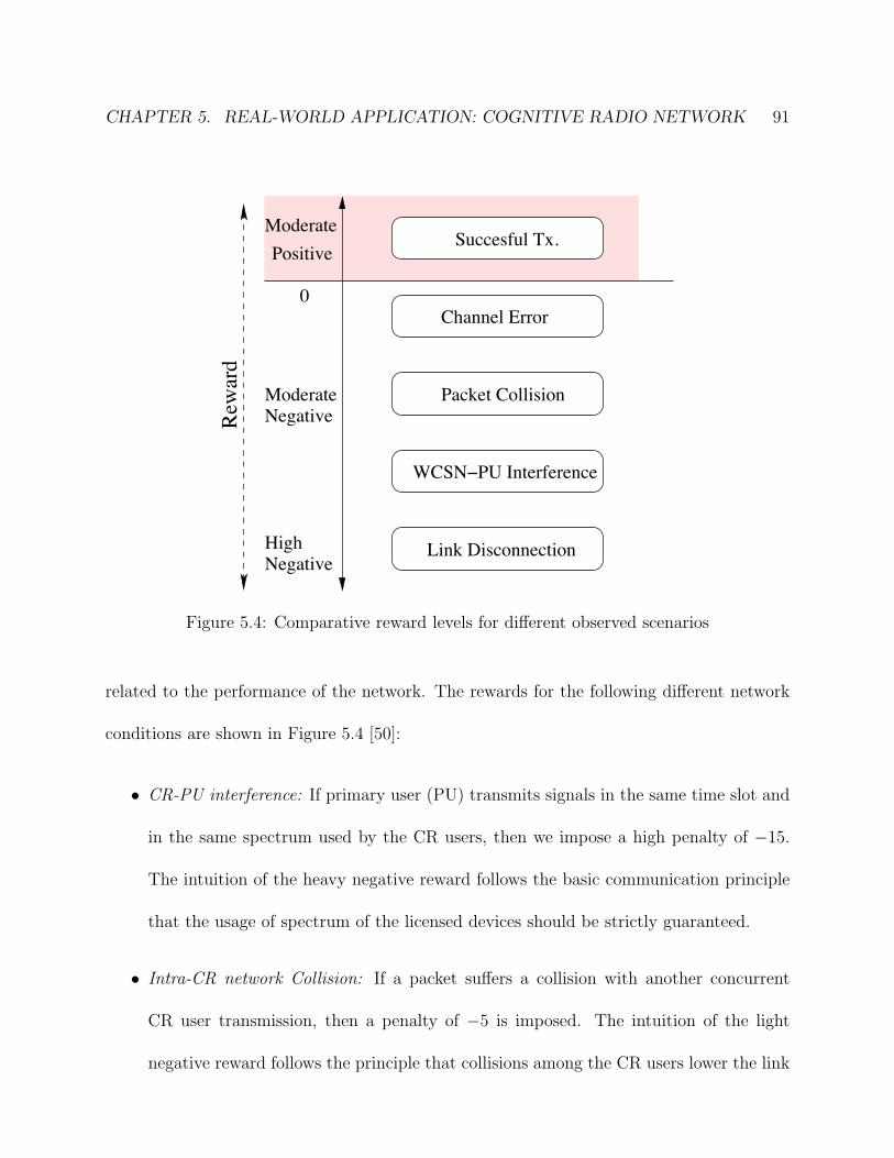
CHAPTER 5. REAL-WORLD APPLICATION: COGNITIVE RADIO NETWORK 91
Succesful Tx.
Channel Error
Packet Collision
WCSN PU Interference
Link Disconnection
ModeratePositive
ModerateNegative
HighNegative
0
Rew
ard
Figure 5.4: Comparative reward levels for different observed scenarios
related to the performance of the network. The rewards for the following different network
conditions are shown in Figure 5.4 [50]:
• CR-PU interference: If primary user (PU) transmits signals in the same time slot and
in the same spectrum used by the CR users, then we impose a high penalty of −15.
The intuition of the heavy negative reward follows the basic communication principle
that the usage of spectrum of the licensed devices should be strictly guaranteed.
• Intra-CR network Collision: If a packet suffers a collision with another concurrent
CR user transmission, then a penalty of −5 is imposed. The intuition of the light
negative reward follows the principle that collisions among the CR users lower the link

CHAPTER 5. REAL-WORLD APPLICATION: COGNITIVE RADIO NETWORK 92
throughput, which should be avoided. The comparatively low penalty to the CR users
arising from intra-network collisions aims to force fair sharing of the available spectrum
by encouraging the users to choose distinct spectrum bands, if available.
• Channel Induced Errors: If a transmitted packet suffers any channel induced error,
then we impose a penalty of −5. The intuition of the light negative reward follows the
principle that certain spectrum bands are more robust to channel errors owing to their
lower attenuation rates. By preferring the spectrum bands with the lowest packet error
rate (PER), the CR users reduce re-transmissions and associated network delays.
• Link Disconnection: If the received power (P jrx) is less than the threshold of the receiver
Prth (here, assumed as −85 dBm), then all the packets are dropped, and we impose a
steep penalty of −20. Thus, the sender should quickly increase its choice of transmit
power so that the link can be re-established.
• Successful Transmission: If none of the above conditions are observed to be true in
the given transmission slot, then packet is successfully transmitted from the sender to
receiver, and a reward of +5 is assigned.
In this way, we can apply multi-agent reinforcement learning to solve cognitive radio
problem [50].

CHAPTER 5. REAL-WORLD APPLICATION: COGNITIVE RADIO NETWORK 93
(Application Layer)
SensingSpectrumSharing
Reinforcement Learning Module
Spectrum Spectrum
CR Link Layer Module
**
SpectrumNeighborList
* Tx Power
CR Physical Layer Module
Block
SpectrumBlock
Cross LayerRepository
PU Activity
(MAC Functionality)
Management
Figure 5.5: Block diagram of the implemented simulator tool for reinforcement learningbased cognitive radio.
5.3 Experimental Simulation
In this section, we describe preliminary results from applying multi-agent reinforcement
learning to our cognitive radio model. The overall aim of our proposed learning based
approach is to allow the CR users (i.e., agents) to decide on an optimal choice of transmission
power and spectrum so that (i) PUs are not affected, and (ii) CR users share the spectrum
in a fair manner.
5.3.1 Simulation Setup
A novel CR network simulator described in Section 4.1 has been designed to investigate the
effect of the proposed reinforcement learning technique on the network’s operation. As shown
in Figure 5.5, our implemented ns-2 model [50] is composed of several modifications to the
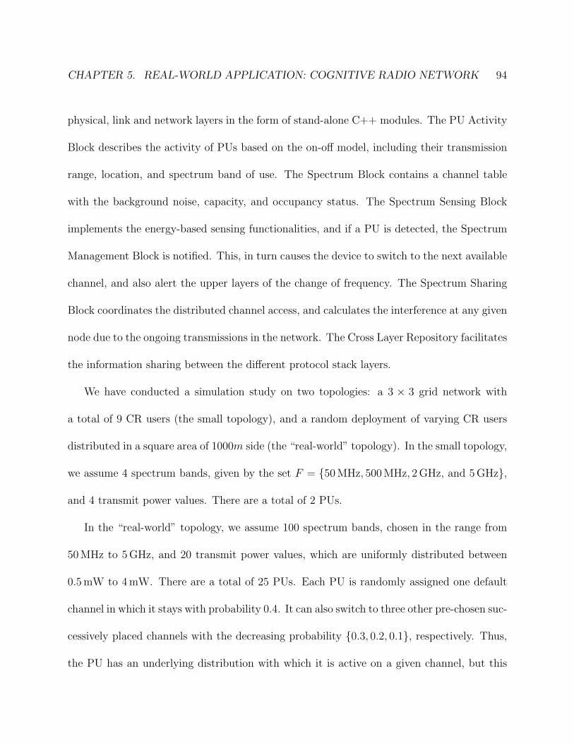
CHAPTER 5. REAL-WORLD APPLICATION: COGNITIVE RADIO NETWORK 94
physical, link and network layers in the form of stand-alone C++ modules. The PU Activity
Block describes the activity of PUs based on the on-off model, including their transmission
range, location, and spectrum band of use. The Spectrum Block contains a channel table
with the background noise, capacity, and occupancy status. The Spectrum Sensing Block
implements the energy-based sensing functionalities, and if a PU is detected, the Spectrum
Management Block is notified. This, in turn causes the device to switch to the next available
channel, and also alert the upper layers of the change of frequency. The Spectrum Sharing
Block coordinates the distributed channel access, and calculates the interference at any given
node due to the ongoing transmissions in the network. The Cross Layer Repository facilitates
the information sharing between the different protocol stack layers.
We have conducted a simulation study on two topologies: a 3 × 3 grid network with
a total of 9 CR users (the small topology), and a random deployment of varying CR users
distributed in a square area of 1000m side (the “real-world” topology). In the small topology,
we assume 4 spectrum bands, given by the set F = {50 MHz, 500 MHz, 2 GHz, and 5 GHz},
and 4 transmit power values. There are a total of 2 PUs.
In the “real-world” topology, we assume 100 spectrum bands, chosen in the range from
50 MHz to 5 GHz, and 20 transmit power values, which are uniformly distributed between
0.5 mW to 4 mW. There are a total of 25 PUs. Each PU is randomly assigned one default
channel in which it stays with probability 0.4. It can also switch to three other pre-chosen suc-
cessively placed channels with the decreasing probability {0.3, 0.2, 0.1}, respectively. Thus,
the PU has an underlying distribution with which it is active on a given channel, but this

CHAPTER 5. REAL-WORLD APPLICATION: COGNITIVE RADIO NETWORK 95
is unknown to the CR user. Transmission in the CR network occurs on multiple sets of
pre-decided node pairs, each such pair forming a link represented as (i, j). The terms in
the parenthesis denote the directional transmission from the sender i to the receiver j. The
choice of spectrum is made by the sender node, and is communicated to the receiver over the
common control channel or CCC. This CCC is also used to return feedback to the sender
regarding possible collisions that may be experienced by the receiver. However, data trans-
mission occurs exclusively in the spectrum chosen by the node pair forming the link. We
consider the time to be slotted, and the link layer at each sender node attempts to transmit
with a probability p = 0.2 in every slot.
We compare the performance of our reinforcement learning based (RL-based) scheme
with three other schemes: (i) random assignment, which selects a random combination of
spectrum and power in each round; (ii) greedy assignment with history 1 (G-1), and (iii)
greedy assignment with history 20 (G-20). The G-1 algorithm stores for every possible
spectrum and power combination the reward received the last time that combination was
selected (if any). The algorithm selects the combination with the highest previous reward
with probability η and explores a randomly chosen combination with probability (1−η). The
G-20 algorithm maintains a repository of the reward obtained in the 20 past slots for every
combination of power and spectrum, and selects the best combination in the past 20 slots.
Similar to G-1, G-20 selects the best known combination from the history with η = 0.8, and
explores a randomly chosen one with probability (1−η) = 0.8. In our RL-based scheme, the
exploration rate ε is set to 0.2, which we found experimentally to give the best results. The

CHAPTER 5. REAL-WORLD APPLICATION: COGNITIVE RADIO NETWORK 96
initial learning rate α is set to 0.8, and it is decreased by a factor of 0.995 after each time
slot. Note that G-1 uses the same amount of memory as the RL-based scheme, but G-20
uses 20 times more memory.
5.3.2 Simulation Evaluation
We apply the four schemes, i.e. random, G-1, G-20, and RL-based, to the small topologies.
We collect the results over 30000 time slots, and record the average probabilities of successful
transmission, the average rewards of CR users, and the average number of channel switches
by CR users. We then plot these values over time. Each experiment is performed 5 times
and we report the means and standard deviations of the recorded values. In our experiments,
all runs were found to converge within 30,000 epochs.
Figure 5.6(a) shows the average probability of successful transmission when applying the
four schemes to the small topology. The results show that the RL-based scheme transmits
successful packets with an average probability of approximately 97.5%, while the G-20, G-1
and random schemes transmit successful packets with average probabilities of approximately
88.2%, 79.4%, and 48.7%, respectively. The results indicate that after learning, the RL-
based approach can effectively guarantee successful transmissions, and its performance is
much better than the others, including the G-20 scheme which uses more than an order of
magnitude more memory.
Figure 5.6(b) shows the corresponding average rewards received by CR users when ap-
plying the four schemes to the small topology. The results show that after learning, the
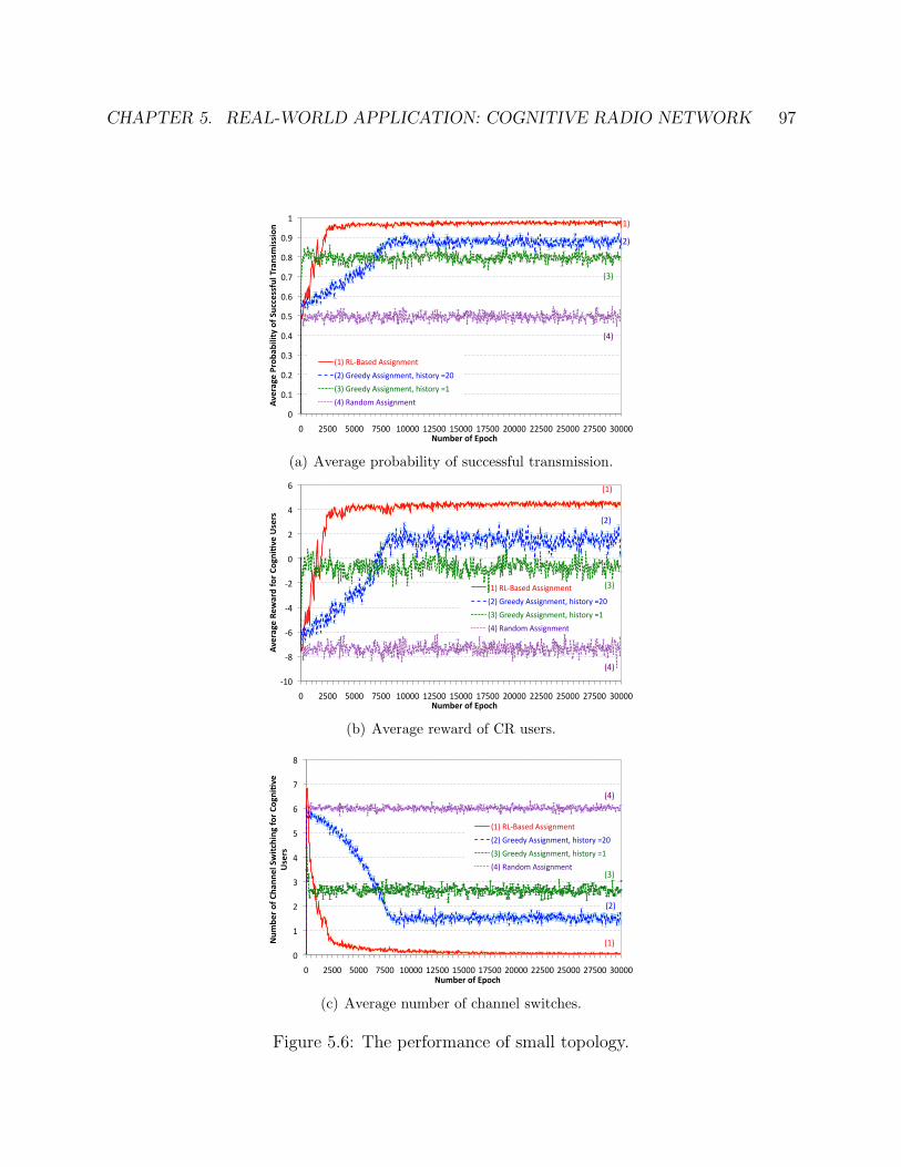
CHAPTER 5. REAL-WORLD APPLICATION: COGNITIVE RADIO NETWORK 97
0
0.1
0.2
0.3
0.4
0.5
0.6
0.7
0.8
0.9
1
0 2500 5000 7500 10000 12500 15000 17500 20000 22500 25000 27500 30000
AverageProba
bilityofSuccessfulTransmission
NumberofEpoch
(1)RL‐BasedAssignment
(2)GreedyAssignment,history=20
(3)GreedyAssignment,history=1
(4)RandomAssignment
(1)
(2)
(3)
(4)
(a) Average probability of successful transmission.
‐10
‐8
‐6
‐4
‐2
0
2
4
6
0 2500 5000 7500 10000 12500 15000 17500 20000 22500 25000 27500 30000
AverageRew
ardforCo
gni0veUsers
NumberofEpoch
(1)RL‐BasedAssignment
(2)GreedyAssignment,history=20
(3)GreedyAssignment,history=1
(4)RandomAssignment
(1)
(2)
(3)
(4)
(b) Average reward of CR users.
0
1
2
3
4
5
6
7
8
0 2500 5000 7500 100001250015000175002000022500250002750030000
Num
berofCha
nnelSwitchingforCo
gni5ve
Users
NumberofEpoch
(1)RL‐BasedAssignment
(2)GreedyAssignment,history=20
(3)GreedyAssignment,history=1
(4)RandomAssignment
(1)
(2)
(3)
(4)
(c) Average number of channel switches.
Figure 5.6: The performance of small topology.

CHAPTER 5. REAL-WORLD APPLICATION: COGNITIVE RADIO NETWORK 98
RL-based scheme receives the largest positive reward of approximately +4.3, while the G-20
gets a reward of approximately +1.7, G-1 gets an negative average reward of approximately
−0.8 and the random scheme gets a negative average reward of approximately −7.5. The
results indicate that the RL-based approach pushes CR users to gradually achieve higher
positive rewards and choose more suitable spectrum and power values for their transmis-
sion. The results also indicate that the reward tends to be proportional to the probability
of successful transmission.
Figure 5.6(c) shows the corresponding average number of channel switches by CR users
when applying the four schemes to solve the small topology. The results show that after
learning, the RL-based scheme tends to eliminate channel switching, while the level of channel
switching by G-20 is approximately 1.5, by G-1 is 2.6, and by the random scheme is 6.0.
The results indicate that our RL-based approach is able to keep the channel switches very
low. The results also indicate that our approach can converge to an optimal solution for
successful transmission after learning.
We further observe in the graphs of Figures 5.6(a), 5.6(b) and 5.6(c) that the behavior
of the RL-based scheme is smoother and more predicatable than the behavior of the other
approaches. These results suggest that our approach is more stable than the G-20, G-1, and
random approaches.
We then applied RL-based scheme to the “real-world” topologies. We focus on five
different node densities, with 100, 200, 300, 400 and 500 nodes randomly placed within a
square area of side 1000m. We collect the results over 60, 000 time slots, and record the

CHAPTER 5. REAL-WORLD APPLICATION: COGNITIVE RADIO NETWORK 99
0
0.1
0.2
0.3
0.4
0.5
0.6
0.7
0.8
0.9
1
0 5000 10000 15000 20000 25000 30000 35000 40000 45000 50000 55000 60000
AverageProbab
ilityofSuccessfulTransm
ission
NumberofEpoch
(1)100nodes
(2)200nodes
(3)300nodes
(4)400nodes
(5)500nodes
(1)(2)(3)
(4)(5)
(a) Average probability of successful transmission.
‐20
‐15
‐10
‐5
0
5
10
0 5000 10000 15000 20000 25000 30000 35000 40000 45000 50000 55000 60000
AverageRewardforCogni0veUsers
NumberofEpoch
(1)100nodes
(2)200nodes
(3)300nodes
(4)400nodes
(5)500nodes
(1)(2)
(3)
(4)(5)
(b) Average reward of CR users.
0
50
100
150
200
250
0 5000 10000 15000 20000 25000 30000 35000 40000 45000 50000 55000 60000
NumberofChan
nelSwitchingforCogni5ve
Users
NumberofEpoch
(5)500nodes
(4)400nodes
(3)300nodes
(2)200nodes
(1)100nodes
(1)(2)(3)
(4)
(5)
(c) Average number of channel switches.
Figure 5.7: The performance of the real-world topology with five different node densities.

CHAPTER 5. REAL-WORLD APPLICATION: COGNITIVE RADIO NETWORK 100
average probabilities of successful transmission, the average rewards of CR users, and the
average number of channel switches by CR users. We then plot these values over time. Each
experiment is performed 5 times and we report the means and standard deviations of the
recorded values.
Figure 5.7(a) shows the average probabilities of successful transmissions when applying
the RL-based to the “real-world” topology. The results show that the RL-based scheme
transmits successful packets with an average probability of approximately 100% within the
topology with 100 nodes, 99.8% within the topology with 200 nodes, 91.6% within the
topology with 300 nodes, 81.3% within the topology with 400 nodes and 79.1% within the
topology with 500 nodes, respectively.
Figure 5.7(b) shows the corresponding average rewards of CR users when applying the
same three schemes to the large topology. The results show that after learning, the RL-based
scheme receives the largest average reward of approximately 5 within the topology with 100
nodes, 4.9 within the topology with 200 nodes, −4.6 within the topology with 300 nodes,
−9.2 within the topology with 400 nodes and −9.9% within the topology with 500 nodes,
respectively.
Figure 5.7(c) shows the corresponding average number of channel switches of CR users
when applying the three schemes to the large topology. The results show that after learning,
the RL-based scheme tends to decrease channel switching to approximately 0 within the
topology with 100 and 200 nodes, 17.4 within the topology with 300 nodes, 45.8 within the
topology with 400 nodes and 61.5 within the topology with 500 nodes respectively.

CHAPTER 5. REAL-WORLD APPLICATION: COGNITIVE RADIO NETWORK 101
In the “real-world” topology, our reinforcement learning technique shows two key char-
acteristics: (1) as the size of the “real-world” topology increases, the performance of the
RL-based scheme decreases. Specifically, the average probabilities of successful transmis-
sions and the average rewards of CR users decrease, and the average number of channel
switches of CR users increases while the number of nodes increases, and (2) as the size of
the “real-world” topology increases, the RL-based scheme needs more time for convergence.
It should be emphasized that the RL-based scheme are subject to complex network behavior
and exhibit different sub-optimal peaks before converging on a static value. We are not
aware of any previously published studies that simulate such large networks.
5.4 Function Approximation for RL-based Cognitive
Radio
RL-based cognitive radio gives better network performance over the other approaches. How-
ever the requirement of RL-based approaches that an estimated value be stored for every
state greatly limits the size and complexity of CR networks that can be solved. For example,
if the number of nodes, spectrum values or transmission power levels is very large, much
more memory and time will be needed to find solutions, typically making the problem more
difficult to solve. The memory required to store such large tables of Q-values can greatly
exceed the memory required for the random and greedy approaches. There is therefore a
need for algorithms to reduce the size of memories be used for large-scale CR networks.

CHAPTER 5. REAL-WORLD APPLICATION: COGNITIVE RADIO NETWORK 102
0
0.1
0.2
0.3
0.4
0.5
0.6
0.7
0.8
0.9
1
0 5000 1000015000200002500030000350004000045000500005500060000
AverageProbab
ilityofSuccessfulTransm
ission
NumberofEpoch
(1)RL‐Based
(2)RL‐K‐Basedwith1500prototypes
(3)RL‐K‐Basedwith1000prototypes
(4)RL‐K‐Basedwith500prototypes
(1)(2)
(3)
(4)
Figure 5.8: Average probability of successful transmission for the real-world topology with500 nodes.
Function approximation is such a well-suited algorithm to solve this problem.
We evaluate our reinforcement learning-based approach with Kanerva-based function
approximation (RL-K-based) by applying it to the “real-world” topology with 500 nodes.
We compare the performance of the RL-K-based scheme with the RL-based scheme. In the
RL-K-based approach, the learning parameters are the same as the RL-based approach. The
number of prototypes for each CR user varies over the following values: 500, 1000, 1500.
Note that the number of states for each CR user in the “real-world” topology is 2000, that
is, 100 (channels) × 20 (power values).
Figure 5.8 shows the average probability of successful transmission when applying the
RL-K-based scheme with varying numbers of prototypes to the large topology. The results
CHAPTER 5. REAL-WORLD APPLICATION: COGNITIVE RADIO NETWORK 103
show that after learning, the RL-K-based scheme with 500, 1000 or 1500 prototypes transmits
successful packets with an average probability of approximately 63.5%, 67.6%, and 78.1%,
respectively. In comparison to the RL-based scheme that uses memory to store 2000 Q-values
for each CR user, the RL-K-based scheme only need 2/3, 1/2, and 1/4 as much memory to
store Q-values for 1500, 1000 or 500 prototypes, respectively. The results indicate that
although the performance of the RL-K-based scheme is worse than the RL-based scheme,
the RL-K-based scheme can use less space to store an approximate of Q-table. For example,
the RL-K-based scheme uses 2/3 as much memory as the pure RL scheme with a loss of only
1.3% of successful transmissions with 1500 prototypes, and uses 1/2 as much memory with
the loss of only 14.5% of successful transmissions with 1000 prototypes. The results also
show that if the number of prototypes is too small, the performance is similar to randomly
choosing channels and power values. In our future work, we will focus on using prototype
optimization techniques to improve the efficiency of Kanerva-based function approximation
for reinforcement learning based cognitive radio.
5.5 Summary
Cognitive radio is a new paradigm that attempts to opportunistically transmit in licensed
frequencies, without affecting the existing primary users of these bands. To realize this ca-
pability, such a radio must predict specific interferer transmission patterns and adaptively
change its operational parameters, such as transmit power and spectrum. These tasks, collec-
tively referred to as spectrum management, are difficult to achieve in a dynamic distributed

CHAPTER 5. REAL-WORLD APPLICATION: COGNITIVE RADIO NETWORK 104
environment. The reinforcement learning-based spectrum management in CR network can
be used to address the issue. However, it often gives poor performance when applied to large-
scale networks. These networks typically have a very large number of unlicensed and licensed
users, and a wide range of possible transmission parameters. There is therefore a need for
algorithms to scale up reinforcement learning for large-scale cognitive radio networks.
In this chapter, we evaluate a spectrum management approach based on multi-agent re-
inforcement learning for CR ad hoc networks with decentralized control. This approach uses
value functions to measure the desirability of choosing different transmission parameters,
and enables efficient assignment of spectrum and transmit powers by maximizing long-term
rewards. We show that the RL-based approach works well for small topology networks and
performs poorly for large topology networks. We then attempt to solve the problem of
sharply decreasing CR network performance as the size of the network increases. We apply
Kanerva-based function approximation techniques to scale up our RL-based spectrum man-
agement for large-scale cognitive radio networks. By evaluating its effect on communication
performance, we showed that function approximation can effectively reduce the memory used
for large networks with little loss of performance. We therefore conclude that our RL-based
spectrum management with Kanerva-based function approximation can significantly reduce
interference to licensed users, while maintaining a high probability of successful transmissions
in a cognitive radio ad hoc network.

Chapter 6
Conclusion
Function approximation can be used to improve the performance of reinforcement learners.
Traditional techniques, including Tile Coding and Kanerva Coding, can give poor perfor-
mance when applied to large-scale problems. In this dissertation, we addressed the issue of
solving large-scale, high-dimension problems using reinforcement learning with function ap-
proximation. We developed novel parametric approximation techniques and corresponding
parameter-tuning methods for achieving better learning performance.
We first reviewed the state-on-the-art of reinforcement learning and function approxima-
tion techniques. We showed that the limiting factor when applying reinforcement learning
to large-scale problems is the size of the table needed to store the state-action values is too
large. Traditional function approximation techniques can be used to reduce the size of the
table. However, their efficiency s is poor when applied to domains that are very large, have
high dimension or that have a continuous state-action space.
105
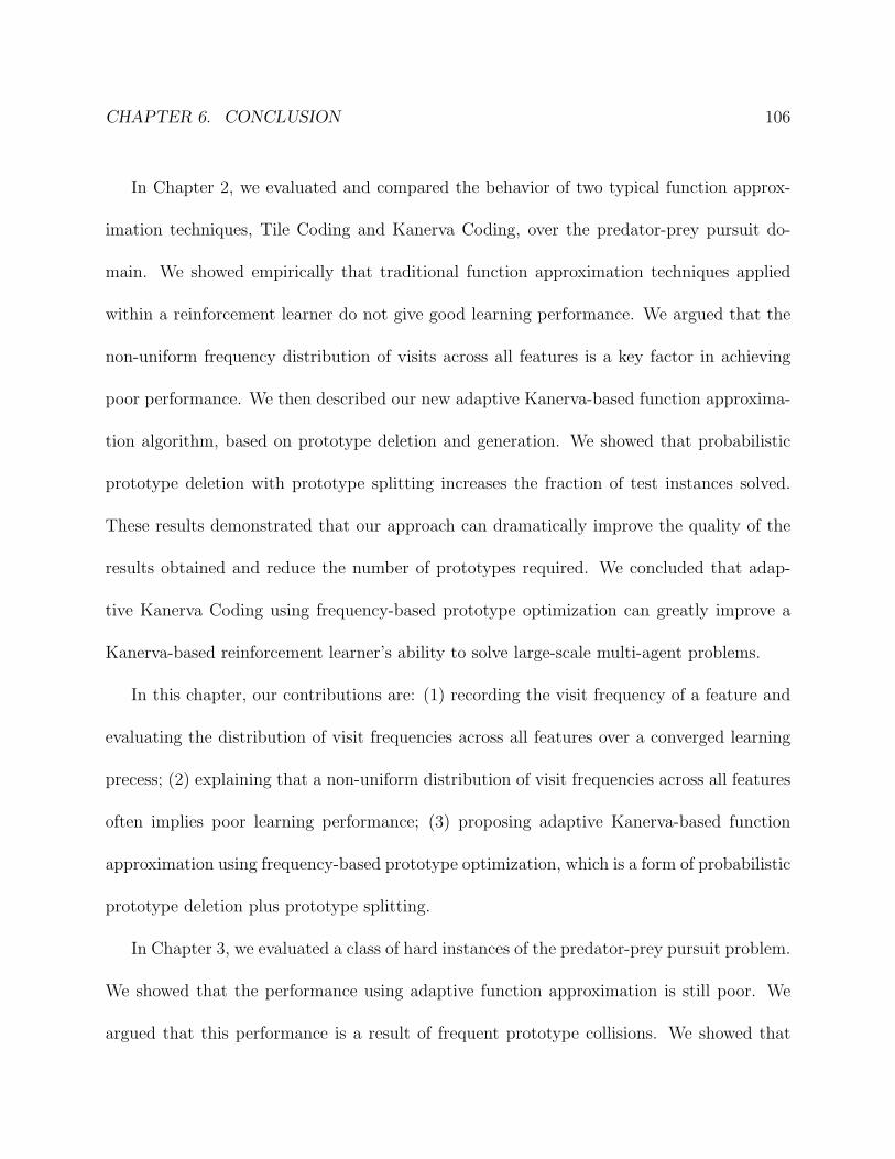
CHAPTER 6. CONCLUSION 106
In Chapter 2, we evaluated and compared the behavior of two typical function approx-
imation techniques, Tile Coding and Kanerva Coding, over the predator-prey pursuit do-
main. We showed empirically that traditional function approximation techniques applied
within a reinforcement learner do not give good learning performance. We argued that the
non-uniform frequency distribution of visits across all features is a key factor in achieving
poor performance. We then described our new adaptive Kanerva-based function approxima-
tion algorithm, based on prototype deletion and generation. We showed that probabilistic
prototype deletion with prototype splitting increases the fraction of test instances solved.
These results demonstrated that our approach can dramatically improve the quality of the
results obtained and reduce the number of prototypes required. We concluded that adap-
tive Kanerva Coding using frequency-based prototype optimization can greatly improve a
Kanerva-based reinforcement learner’s ability to solve large-scale multi-agent problems.
In this chapter, our contributions are: (1) recording the visit frequency of a feature and
evaluating the distribution of visit frequencies across all features over a converged learning
precess; (2) explaining that a non-uniform distribution of visit frequencies across all features
often implies poor learning performance; (3) proposing adaptive Kanerva-based function
approximation using frequency-based prototype optimization, which is a form of probabilistic
prototype deletion plus prototype splitting.
In Chapter 3, we evaluated a class of hard instances of the predator-prey pursuit problem.
We showed that the performance using adaptive function approximation is still poor. We
argued that this performance is a result of frequent prototype collisions. We showed that

CHAPTER 6. CONCLUSION 107
dynamic prototype allocation and adaptation can partially reduce these collisions and give
better results than traditional function approximation. To completely eliminate prototype
collisions, we then described a novel fuzzy approach to Kanerva-based function approxi-
mation which uses a fine-grained fuzzy membership grade to describe a state-action pair’s
adjacency with respect to each prototype. This approach, coupled with adaptive prototype
allocation, allows the solver to distinguish membership vectors and reduce the collision rate.
We also showed that reducing the similarity between the membership vectors of state-action
pairs can give better results. We used Maximum Likelihood Estimation to adjust the vari-
ance of basis functions and tune the receptive fields of prototypes. Finally, we concluded
that our adaptive fuzzy Kanerva approach with prototype tuning gives better performance
than the pure adaptive Kanerva algorithm.
In this chapter, our contributions are: (1) introducing prototype collision and analyzing
the cause of prototype collision; (2) explaining that frequent prototype collisions are the key
factor that reduces the performance of function approximation; (3) proposing fuzzy Kanerva-
based function approximation, coupled with adaptive prototype allocation; (4) revealing that
the similarity between the membership vectors of state-action pairs has a similar effect to
prototype collision; (5) proposing the prototype tuning method to reduce the similarity
between the membership vectors of state-action pairs.
In Chapter 4, we evaluated adaptive Kanerva coding using frequency-based prototype
optimization by applying it to solve a class of hard instances of the predator-prey pursuit
problem. We showed that the poor performance is caused by an inappropriate selection
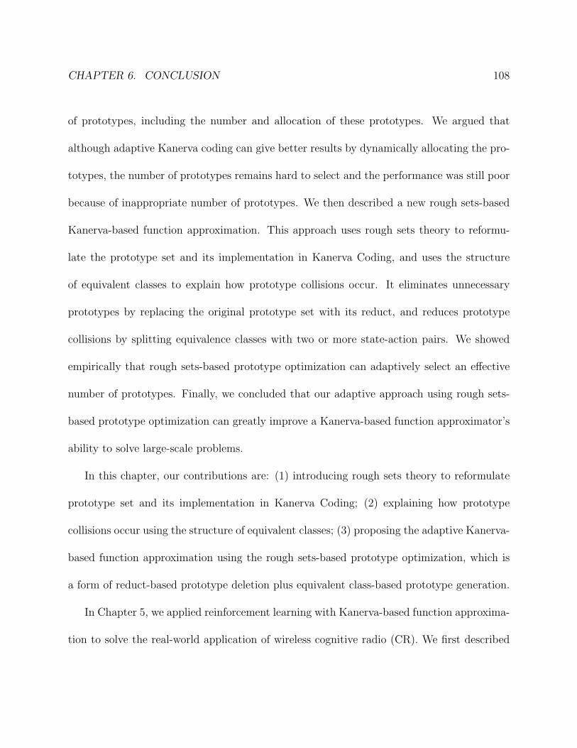
CHAPTER 6. CONCLUSION 108
of prototypes, including the number and allocation of these prototypes. We argued that
although adaptive Kanerva coding can give better results by dynamically allocating the pro-
totypes, the number of prototypes remains hard to select and the performance was still poor
because of inappropriate number of prototypes. We then described a new rough sets-based
Kanerva-based function approximation. This approach uses rough sets theory to reformu-
late the prototype set and its implementation in Kanerva Coding, and uses the structure
of equivalent classes to explain how prototype collisions occur. It eliminates unnecessary
prototypes by replacing the original prototype set with its reduct, and reduces prototype
collisions by splitting equivalence classes with two or more state-action pairs. We showed
empirically that rough sets-based prototype optimization can adaptively select an effective
number of prototypes. Finally, we concluded that our adaptive approach using rough sets-
based prototype optimization can greatly improve a Kanerva-based function approximator’s
ability to solve large-scale problems.
In this chapter, our contributions are: (1) introducing rough sets theory to reformulate
prototype set and its implementation in Kanerva Coding; (2) explaining how prototype
collisions occur using the structure of equivalent classes; (3) proposing the adaptive Kanerva-
based function approximation using the rough sets-based prototype optimization, which is
a form of reduct-based prototype deletion plus equivalent class-based prototype generation.
In Chapter 5, we applied reinforcement learning with Kanerva-based function approxima-
tion to solve the real-world application of wireless cognitive radio (CR). We first described

CHAPTER 6. CONCLUSION 109
multi-agent reinforcement learning-based spectrum management. We showed that the RL-
based approach works well for small topology networks and performs poorly for large topol-
ogy networks. We argued that the decreasing performance of CR networks is a result of the
increasing network size. We then applied Kanerva-based function approximation techniques
to scale up our RL-based spectrum management for large-scale cognitive radio networks. By
evaluating its effect on communication performance, we showed that function approximation
can effectively reduce the memory used for large networks with little loss of performance. We
therefore concluded that our RL-based spectrum management with Kanerva-based function
approximation can significantly reduce interference to licensed users, while maintaining a
high probability of successful transmissions in a cognitive radio ad hoc network.
In this chapter, our contributions are: (1) proposing a spectrum management approach
based on multi-agent reinforcement learning; (2) demonstrating that the sharply decreasing
performance of CR networks is a result of increasing network size; (3) applying Kanerva-
based function approximation techniques to scale up our RL-based spectrum management.
In conclusion, this dissertation addressed the issue of solving large-scale, high-dimension
problems using reinforcement learning with function approximation. We developed novel
parametric approximation techniques and corresponding parameter-tuning methods for achiev-
ing better learning performance. We applied function approximation techniques to solve the
instances from the predator-pray pursuit domain and cognitive radio network domain. We
conclude that our novel Kanerva-based function approximation techniques can greatly im-
prove the ability of a reinforcement learner to solve large-scale problems.

Bibliography
[1] Fcc adopts rules for unlicensed use of television white spaces. FCC press release, Novem-
ber 2008.
[2] D. Wunsch A. Gorban, B. Kegl and A. Zinovyev. Principal manifolds for data visual-
isation and dimension reduction. In LNCSE 58, Springer, Berlin - Heidelberg - New
York, 2007. ISBN 978-3-540-73749-0, 2007.
[3] M. Adler, H. Racke, N. Sivadasan, C. Sohler, and B. Vocking. Randomized pursuit-
evasion in graphs. In Proc. of the Intl. Colloq. on Automata, Languages and Program-
ming, 2002.
[4] Ian F. Akyildiz, Won-Yeol Lee, and Kaushik Chowdhury. CRAHNs: Cognitive Radio
Ad Hoc Networks. Ad Hoc Networks Journal (Elsevier), 7(5):810–836, July 2009.
[5] Ian F. Akyildiz, Won-Yeol Lee, Mehmet C. Vuran, and Shantidev Mohanty. NeXt
Generation/Dynamic Spectrum Access/Cognitive Radio Wireless Networks: A Survey.
Computer Networks Journal(Elsevier), 50:2127–2159, September 2006.
[6] J. Albus. Brains, Behaviour, and Robotics. McGraw-Hill, 1981.
110

BIBLIOGRAPHY 111
[7] D. Ashlock. Evolutionary computation for modeling and optimization. In Springer,
ISBN 0-387-22196-4., 2006.
[8] S. Thrun B. P. Gerkey and G. Gordon. Visibility-based pursuit-evasion with limited
field of view. In Proc. of the Natl. Conf. on Artificial Intelligence (AAAI), 2004.
[9] T. Back. Evolutionary algorithms in theory and practice: Evolution strategies. In
Evolutionary Programming, Genetic Algorithms, Oxford Univ. Press., 1996.
[10] L. Baird. Residual algorithms: Reinforcement learning with function approximation. In
Proc. of the 12th Intl. Conf. on Machine Learning. Morgan Kaufmann, 1995.
[11] L. Baird and A. Moore. Gradient descent for general reinforcement learning. In Advances
in Neural Information Processing Systems 11, 1999.
[12] R. Bellman and S. E. Dreyfus. Functional approximations and dynamic programming.
In Math Tables and Other Aides to Computation, 13:247-251., 1959.
[13] H. R. Berenji and D. Vengerov. On convergence of fuzzy reinforcement learning. In
Proc. of FUZZ-IEEE 2001, 2001.
[14] N. Cristianini and J. Shawe-Taylor. An introduction to support vector machines and
other kernel-based learning methods. In Cambridge University Press, 2000. ISBN 0-
521-78019-5, 2000.
[15] A.E. Eiben and J.E. Smith. Introduction to evolutionary computing. In Springer, 2003.

BIBLIOGRAPHY 112
[16] P. Glorennec. Fuzzy q-learning and dynamical fuzzy q-learning. In IEEE International
Conference on Fuzzy Systems, 1994.
[17] G. J. Gordon. Stable function approximation in dynamic programming. In Proc. of
International Conference on Machine Learning, 1995.
[18] S. Haykin. Cognitive Radio: Brain-empowered Wireless Communications. IEEE Journal
on Selected Areas in Communications, 23(2):201–220, July 2005.
[19] T. Haynes and S. Sen. The evolution of multiagent coordination strategies. Adaptive
Behavior, 1997.
[20] G. Hinton. Distributed representations. Technical Report, Department of Computer
Science, Carnegie-Mellon University, Pittsburgh, 1984.
[21] V. Isler, S. Kannan, and S. Khanna. Randomized pursuit-evasion with local visibility.
SIAM Journal on Discrete Mathematics, 20(1):26–41, 2006.
[22] Jolliffe I.T. Principal component analysis. In Series: Springer Series in Statistics, 2nd
ed., Springer, NY, 2002, XXIX, 487 p. 28 illus. ISBN 978-0-387-95442-4, 2002.
[23] P. Kanerva. Sparse Distributed Memory. MIT Press, 1988.
[24] P. Kanerva. Sparse distributed memory and related models. 1993.
[25] P. W. Keller, S. Mannor, and D. Precup. Automatic basis function construction for ap-
proximate dynamic programming and reinforcement learning. In Proc. of International
Conference on Machine Learning, 2006.

BIBLIOGRAPHY 113
[26] K. Kostiadis and H. Hu. Kabage-rl: kanerva-based generalisation and reinforcement
learning for possession football. In Proc. of IEEE/RSJ Intl. Conf. on Intelligent Robots
and Systems, 2001.
[27] M. G. Lagoudakis and R. Parr. Least-squares policy iteration, issue 4, 1107-1149. In
Journal of Machine Learning Research, 2003.
[28] V. Jagannathan M. Benda and R. Dodhiawala. On optimal cooperation of knowledge
sources - an empirical investigation. In Boeing Advanced Technology Center, Boeing
Computing Services, Seattle, Washington, 1986.
[29] J. Mitola. Cognitive Radio for Flexible Mobile Multimedia Communication. In Proc.
IEEE International Workshop on Mobile Multimedia Communications (MoMuC) 1999,
pages 3–10, November 1999.
[30] Joseph Mitola and Gerald Q. Maguire. Cognitive radio: Making software radios more
personal. In IEEE Personal Communications, 1999.
[31] R. Munos and A. Moore. Variable resolution discretization in optimal control. Machine
Learning, 2002.
[32] M. L. Puterman. Markov decision processes. In Wiley, 1994.
[33] S. Hutchinson R. Murrieta-Cid, R. Monroy and J. P. Laumond. Complexity result for
the pursuit-evasion game of maintaining visibility of a moving evader. In Robotics and
Automation, 2008. ICRA 2008. IEEE International Conference on, 2008.
BIBLIOGRAPHY 114
[34] B. Ratitch and D. Precup. Sparse distributed memories for on-line value-based rein-
forcement learning. In Proc. of the European Conf. on Machine Learning, 2004.
[35] T. W. Rondeau, M. F. D’Souza, and D. G. Sweeney. Residential microwave oven
interference on bluetooth data performance. IEEE Trans. on Consumer Electronics,
50(3):856–863, August 2004.
[36] P. Stone and M. Veloso. Towards collaborative and adversarial learning: A case study in
robotic soccer. In International Journal of Human-Computer Systems (IJHCS), 1997.
[37] P. Stone and M. Veloso. Multiagent systems: A survey from a machine learning per-
spective. Autonomous Robots, 8(3):345–383, 2000.
[38] R. Sutton and A. Barto. Reinforcement Learning: An Introduction. Bradford Books,
1998.
[39] Richard S. Sutton and Steven D. Whitehead. Online learning with random representa-
tions. In ICML, pages 314–321, 1993.
[40] R.S. Sutton. Generalization in reinforcement learning: Successful examples using sparse
coarse coding. In Proceedings of the 1995 Conference on Advances in Neural Information
Processing Systems, 1995.
[41] R.S. Sutton, D. Precup, and S. Singh. Between mdps and semi-mdps: A framework for
temporal abstration in reinforcement learning. In Artificial Intelligence, 112(1-2):181-
211, 1999.
BIBLIOGRAPHY 115
[42] M. Tan. Multi-agent reinforcement learning: Independent vs. cooperative learning. In
Michael N. Huhns and Munindar P. Singh, editors, Readings in Agents, pages 487–494.
Morgan Kaufmann, CA, 1997.
[43] C. K. Tham. Online function approximation for scaling up reinforcement learning. In
Department of Engineering, University of Cambridge, UK, 1994.
[44] L. Tokarchuk, J. Bigham, and L. Cuthbert. Fuzzy sarsa: An approach to fuzzifying
sarsa learning. In Intl. Conf. on Computational Intelligence for Modelling, Control and
Automation, 2004.
[45] J. N. Tsitsiklis and B. Van Roy. An analysis of temporal-difference learning with function
approximation. In IEEE Transactions on Automatic Control, 1997.
[46] M. D. Waltz and K. S. Fu. A heuristic approach to reinforcment learning control systems.
In IEEE Transactions on Automatic Control, 10:390-398., 1965.
[47] C.J.C.H. Watkins. Learning from delayed rewards. Ph.D thesis, Cambridge Univeristy,
Cambridge, England, 1989.
[48] C. Wu and W. Meleis. Function approximations using tile and kanerva coding for multi-
agent systems. In Proc. Of Adaptive Learning Agents Workshop (ALA) in AAMAS,
2009.
BIBLIOGRAPHY 116
[49] C. Wu and W. Meleis. Fuzzy kanerva-based function approximation for reinforcement
learning. In Proc. Of 8th International Conference on Autonomous Agents and Multia-
gent Systens (AAMAS), 2009.
[50] C. Wu and W. Meleis. Spectrum management of cognitive radio using multi-agent
reinforcement learning. In Proc. Of 9th International Conference on Autonomous Agents
and Multiagent Systens (AAMAS), 2010.