Notes on Thermodynamics and Statistical Physics

Andrew Forrester January 28, 2009

Contents

1 Questions and Ideas 2

2 The Big Picture 2

3 Notation and Conventions 4

4 Mathematical Techniques 5

5 Terms 65.1 Overview . . . . . . . . . . . . . . . . . . . . . . . . . . . . . . . . . . . . . . . . . . . . . . 65.2 Fundamental Thermodynamic Vocabulary . . . . . . . . . . . . . . . . . . . . . . . . . . . . 75.3 Thermodynamic Quantities . . . . . . . . . . . . . . . . . . . . . . . . . . . . . . . . . . . . 135.4 Statistical Mechanics Terms . . . . . . . . . . . . . . . . . . . . . . . . . . . . . . . . . . . . 175.5 Quantities Defined for Proofs . . . . . . . . . . . . . . . . . . . . . . . . . . . . . . . . . . . 215.6 Comments on Terms . . . . . . . . . . . . . . . . . . . . . . . . . . . . . . . . . . . . . . . . 215.7 More Thermodynamic Quantities . . . . . . . . . . . . . . . . . . . . . . . . . . . . . . . . . 21

6 Laws and Relations 22

7 People and Old Eponymous Laws 26

8 Theorems, Postulates, Hypotheses, and Demons 278.1 Proving Theorems . . . . . . . . . . . . . . . . . . . . . . . . . . . . . . . . . . . . . . . . . 29

9 Important Physical Systems, Phenomena, and Applications 29

10 Models, Paradoxes, and Catastrophes 30

11 Advanced or Additional Topics, (Beyond These Notes?) 33

12 Open Questions and Mysteries 34

13 Constants and Important Quantities 34

14 Problem-Solving Issues 34

1

1 Questions and Ideas

Books to Read

• Perhaps Kolmogorov: Ergodic Motion• The Logic of Thermostatistical Physics: QC311.5 .E63 2002

What About?

• (Reif Ch 15) Irreversible processes and Fluctuations, magnetic resonance, Brownian motion and theLangevin equation, Nyquist’s theorem, Onsager relations• Law of mass action• ...

Questions

• One of the major confusions seems to be that functions of different variables are written with the samesymbol. For example, N = N(T, P ) and N = N(µ, ?)Can we fix this problem?• Does temperature mean average energy per k per degree of freedom? (cf. Equipartition Theorem)• Does entropy mean the number of degrees of freedom, or “heat” degrees of freedom, or something else?

When dS = dQ/T , dQ is the change in energy due to heat (or change in heat energy, if one can saythat), and T could be proportional to the energy per degree of freedom.• Does chemical potential mean average energy per particle? or per interaction between particles?• If a usual mercury-filled thermometer is placed in a vacuum, what should it read? (I guess it should

read whatever it read before it was placed in the vacuum, but slowly mercury vapor and atoms mayleak out.)• If a person (37 C) is placed in a very dilute gas that is at (37 C), that person will not remain at the

same temperature, since it will transpirate or transpire, losing heat, and perhaps explode. Right?

2 The Big Picture

Thermodynamics is concerned with the relationship between thermal, mechanical, and chemical (and per-haps electromagnetic) interactions and equilibria (and small fluctuations about equilibria?) on a macro-scopic scale. It describes macroscopic behavior of systems but does not always describe mechanisms behindthat behavior. (Does statistical physics always describe mechanisms? I don’t think so...)Define: kinetics and statistical physics proper (statistical mechanics, “statistical thermodynamics” (Reifpg 124))

Various approaches to thermodynamics: macroscopic/historical, (modern) micro-statistical, (macro-scopic?) variational (Callen’s approach, postulating the maximization of some state function S)

Callen says that “thermodynamics is the study of the restrictions on the possible properties of matterthat follow from the symmetry properties of the fundamental laws of physics.” (This statement seems tolink thermodynamics with statistical physics and modernize the term.)

From http://www.jgsee.kmutt.ac.th/exell/Thermo/Systems.html, Thermodynamics:The theory is restricted to closed thermodynamic systems. A closed thermodynamic system is a quantity

of matter separated from its environment by a container. The system has a set of equilibrium states. Theseequilibrium states are the basic elements of the theory.

2

A transition is a change from one equilibrium state to another. The theory is about what transitionsare possible and what energy exchanges occur between the system and its environment during transitions.During a transition a system may pass through non-equilibrium states. In such cases the theory deals onlywith the relation between the end states and with the total effect of the transition; it cannot deal with thenon-equilibrium states between the end states.

Domains

• Deterministic versus Statistical (or Analytic versus Statistical)• Microscopic versus Macroscopic• Thermodynamic limit (number of particles/atoms/molecules →∞, or & Avogadro’s number)− manipulating factorials arising from Boltzmann’s formula for the entropy, S = k log W, by using

Stirling’s approximation, which is justified only when applied to large numbers.− In some simple cases, and at thermodynamic equilibrium, the results can be shown to be a con-

sequence of the additivity property of independent random variables; namely that the variance ofthe sum is equal to the sum of the variances of the independent variables. In these cases, thephysics of such systems close to the thermodynamic limit is governed by the central limit theoremin probability.

− Fluctuations become negligible for most quantities (except for scattering of light, or near the criticalpoint, or in electronics with shot noise and Johnson-Nyquist noise, or near absolute zero with Bose-Einstein condensation, superconductivity and superfluidity.)

− It is at the thermodynamic limit that the additivity property of macroscopic extensive variables isobeyed. That is, the entropy of two systems or objects taken together (in addition to their energyand volume) is the sum of the two separate values.

• Non-relativistic, Relativistic, and Super-relativistic• Classical versus (Quantum or something else. . . since quantum systems are sometimes described as

classical or semi-classical)

− One obtains in the classical approx. Z =∫· · ·∫e−β E(q1,...,pf ) dq1···dpf

h0f (Reif pg 238)

Historical Development of Theory

Can I break Thermo into a set of theories? (Particle/Atomic Theory of Matter or “Quantum” Theory ofMatter or “Quantum” Theory of “Wavicles” or “Quanta”, Kinetic Theory of Heat, Blah-blah Theory ofEnergy (and/or Energy Exchange), Conservation of Energy, . . . )• Phlogiston Theory (∼1669 – )

− The Idea:− Creators: J.J. Becher, Georg Ernst Stahl: theory of combustion involving combustible earth, or

phlogiston−

• Caloric Theory (∼1783 – )

− The Idea:− 1783 - Antoine Lavoisier deprecates the phlogiston theory and proposes a caloric theory− Proponents: John Dalton, Sadi Carnot (analyzed engines using caloric theory), Emile Clapeyron− Detractors:

3

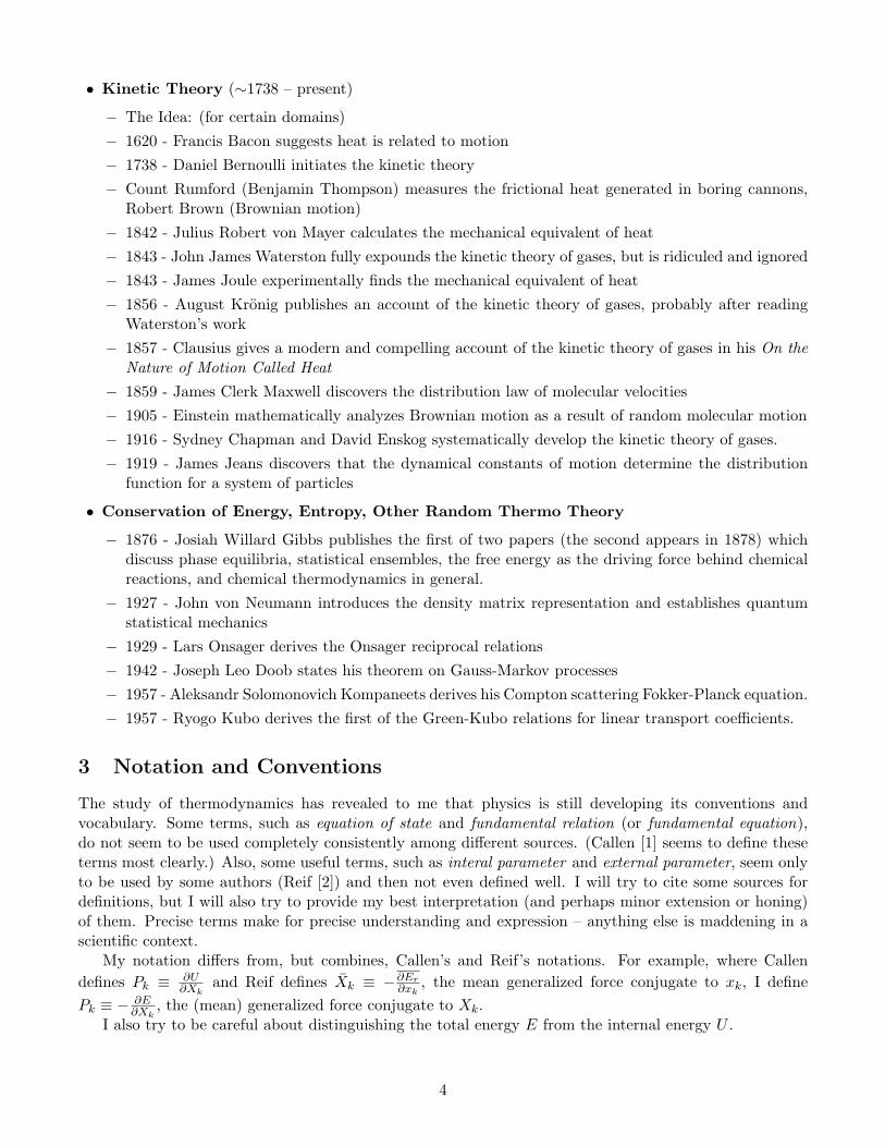
• Kinetic Theory (∼1738 – present)

− The Idea: (for certain domains)− 1620 - Francis Bacon suggests heat is related to motion− 1738 - Daniel Bernoulli initiates the kinetic theory− Count Rumford (Benjamin Thompson) measures the frictional heat generated in boring cannons,

Robert Brown (Brownian motion)− 1842 - Julius Robert von Mayer calculates the mechanical equivalent of heat− 1843 - John James Waterston fully expounds the kinetic theory of gases, but is ridiculed and ignored− 1843 - James Joule experimentally finds the mechanical equivalent of heat− 1856 - August Kronig publishes an account of the kinetic theory of gases, probably after reading

Waterston’s work− 1857 - Clausius gives a modern and compelling account of the kinetic theory of gases in his On the

Nature of Motion Called Heat− 1859 - James Clerk Maxwell discovers the distribution law of molecular velocities− 1905 - Einstein mathematically analyzes Brownian motion as a result of random molecular motion− 1916 - Sydney Chapman and David Enskog systematically develop the kinetic theory of gases.− 1919 - James Jeans discovers that the dynamical constants of motion determine the distribution

function for a system of particles

• Conservation of Energy, Entropy, Other Random Thermo Theory

− 1876 - Josiah Willard Gibbs publishes the first of two papers (the second appears in 1878) whichdiscuss phase equilibria, statistical ensembles, the free energy as the driving force behind chemicalreactions, and chemical thermodynamics in general.

− 1927 - John von Neumann introduces the density matrix representation and establishes quantumstatistical mechanics

− 1929 - Lars Onsager derives the Onsager reciprocal relations− 1942 - Joseph Leo Doob states his theorem on Gauss-Markov processes− 1957 - Aleksandr Solomonovich Kompaneets derives his Compton scattering Fokker-Planck equation.− 1957 - Ryogo Kubo derives the first of the Green-Kubo relations for linear transport coefficients.

3 Notation and Conventions

The study of thermodynamics has revealed to me that physics is still developing its conventions andvocabulary. Some terms, such as equation of state and fundamental relation (or fundamental equation),do not seem to be used completely consistently among different sources. (Callen [1] seems to define theseterms most clearly.) Also, some useful terms, such as interal parameter and external parameter, seem onlyto be used by some authors (Reif [2]) and then not even defined well. I will try to cite some sources fordefinitions, but I will also try to provide my best interpretation (and perhaps minor extension or honing)of them. Precise terms make for precise understanding and expression – anything else is maddening in ascientific context.

My notation differs from, but combines, Callen’s and Reif’s notations. For example, where Callendefines Pk ≡ ∂U

∂Xkand Reif defines Xk ≡ −∂Er

∂xk, the mean generalized force conjugate to xk, I define

Pk ≡ − ∂E∂Xk

, the (mean) generalized force conjugate to Xk.I also try to be careful about distinguishing the total energy E from the internal energy U .

4

Context-dependent equalities: (Perhaps I’ll use this...) In general, a quantity is not the same as itsaverage (over (a local interval of) time and space). But occasionally, I will equate the two when it isappropriate and not mention that I am doing so. In those cases, it would be nice if I would give someindication that the equality is context-dependent: In general Pk 6= Pk, but sometimes when it is true thatPk ≈ Pk, and Pk is equal to some function f , I’ll write Pk

c= f .Possible ambiguities: Some quantities may be defined several different (consistent) ways. Some quanti-

ties may go by several different names. (There may be overlap in names for different quantities (magneticfield).) Some quantities do not have standardized definitions, names, or symbols. (Fermi energy?) Somequantities are commonly represented with the same symbols. (µ; chemical potential or Joule-Thompsoncoefficient.) Some quantities are often represented by several different symbols in different contexts. (“Oc-cupancy” ns, f(ε))

Less ambiguity: Other terms are much less ambiguous. ()

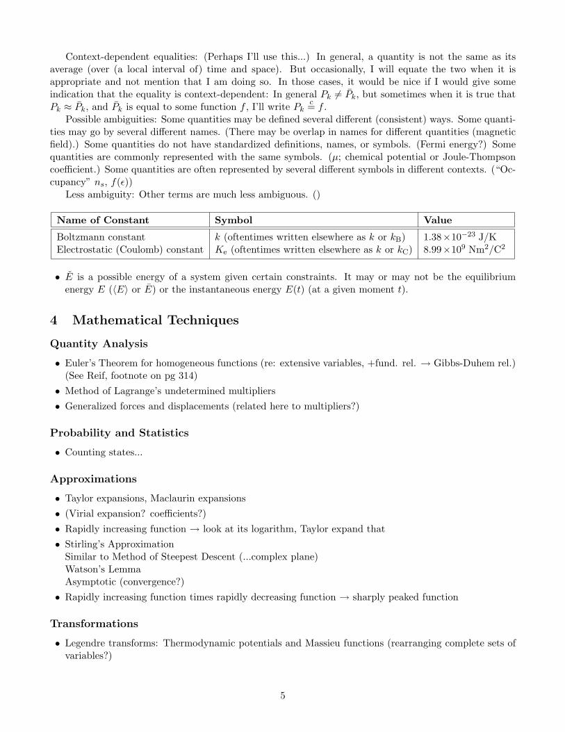
Name of Constant Symbol Value

Boltzmann constant k (oftentimes written elsewhere as k or kB) 1.38×10−23 J/KElectrostatic (Coulomb) constant Ke (oftentimes written elsewhere as k or kC) 8.99×109 Nm2/C2

• E is a possible energy of a system given certain constraints. It may or may not be the equilibriumenergy E (〈E〉 or E) or the instantaneous energy E(t) (at a given moment t).

4 Mathematical Techniques

Quantity Analysis

• Euler’s Theorem for homogeneous functions (re: extensive variables, +fund. rel. → Gibbs-Duhem rel.)(See Reif, footnote on pg 314)• Method of Lagrange’s undetermined multipliers• Generalized forces and displacements (related here to multipliers?)

Probability and Statistics

• Counting states...

Approximations

• Taylor expansions, Maclaurin expansions• (Virial expansion? coefficients?)• Rapidly increasing function → look at its logarithm, Taylor expand that• Stirling’s Approximation

Similar to Method of Steepest Descent (...complex plane)Watson’s LemmaAsymptotic (convergence?)• Rapidly increasing function times rapidly decreasing function → sharply peaked function

Transformations

• Legendre transforms: Thermodynamic potentials and Massieu functions (rearranging complete sets ofvariables?)

5

General 1-D form: Y (X) → ψ(P ) = Y − PX ≡ Y [P ] (= Y (X)− PX?), P ≡ dYdX

What’s the difference between a Legendre transform and taking a derivative?How can you tell what the independent variables are?P ≡ dY/dX, Y (X)→ U(P ) = Y − PX = Y (X)− PX ???U(P, Y,X) ???Compare to multidimensional forms.• ...

Partial Differential Equations

• Maxima, (Calculus of variations?) and the method of Lagrange multipliers (→ conjugate variables,maximizing energies and entropies?)• Flipping derivatives, Jacobians, etc.

− Given three variables x, y, and z, two of which are independent, such that there are functionalrelationships z = z(x, y) and x = x(y, z), then(

∂x

∂y

)z

= − (∂z/∂y)x(∂z/∂x)y(

∂x

∂z

)y

=1

(∂z/∂x)y

− See a case where “the partial derivatives [∂x′/∂x] and [∂x/∂x′ ] are not the algebraic reciprocals ofeach other” here: http://www.mathpages.com/home/kmath024/kmath024.htm

• Bridgman’s Thermodynamic equations (technique)

5 Terms

5.1 Overview

• Fundamental Thermodynamic Vocabulary− Systems and States− State Parameters and their relationships and contraints− Thermodynamic processes− Equilibria and the Fundamental Thermodynamic Postulate

• Thermodynamic Quantities− Energy, Work (←?chemical potential?→) and Heat− Heat, Entropy, and Temperature− Auxiliary Energy and Entropy Functions

• Statistical Mechanics Terms− Number of States, Density of States− Probability density (functions) (e.g. “distribution function”)− Number of particles per state → occupancy function− Mean value of a parameter− (5+) Statistical Ensembles

6

− Partition Functions, Boltzmann Factor− (3+) “Statistics”, etc.

• Symbols Defined for Proofs, Comments on Terms, More Thermodynamic Quantities

5.2 Fundamental Thermodynamic Vocabulary

• System - A physical system is simply a set of physical objects, real or imagined. Systems andtheir constraints usually must be well-defined (using parameters) if precise statements are to madeabout them. We consider properties and phenomena at different spatial scales: macroscopic andmicroscopic scales. Since we assume systems are made of atoms or particles, these scale distinctionsare important. We also consider various temporal scales (e.g., time intervals required for thermalequilibration within or among systems, called “relaxation times”, or time intervals of experimentalinterest). (What about energy scales, etc?)

– The complement of a physical system, i.e., all physical objects in the universe other than thosein the sytem, is often called that system’s environment. Let’s define “environment” as such.(The word “environment” sometimes connotes “immediate environment”, but that is not whatis meant here, so be careful.)

– An isolated system is a system that does not interact with its environment; no external forcesact upon it and no energy or matter is exchanged with its environment. (I should probably becareful about such strange phrases as energy “leaving, crossing boundaries, flowing” etc.)Constant total energy, an isolated system has.

– A thermally isolated or thermally insulated system is a system that cannot interactthermally with its environment and can only interact mechanically. I.e., it may only interact viawork, with changing external parameters, and not via heat, with changing internal parameters(Reif?).An adiabatic boundary, barrier, or envelope prevents heat flow, thermally isolating the system,and allows only adiabatic processes to occur.

– A mechanically isolated system is a system that cannot interact mechanically (throughmacroscopic work) and can only interact thermally.(Constant “external” energy, a mechanically isolated system has?)

– A closed system (or energetically closed system?) is a system that cannot exchange matter orinternal energy with its environment, while there may be external forces (and change in totalenergy)... (see Callen pg 17,26)Constant internal energy, a closed system has.

– A materially closed system1 is a system in which no matter is exchanged with its environ-ment. (There may be external forces and energy may be exchanged (in the form of heat orwork, the only means of exchange by Reif’s definition).) (In the context of chemistry, this isoften called simply a closed system.)(The mass of a materially closed system may change if there are nuclear reactions or particledecays, i.e., radioactivity.)

– A simple system is defined by Callen as a system that is macroscopically homogeneous,isotropic, and uncharged, that is large enough so that surface effects can be neglected, andthat is not acted on by electric, magnetic, or gravitational fields. (This type of system is mostoften the focus of thermodynamics texts.)

1I haven’t seen this term yet.

7

– A composite system is a collection of simple systems. (From Callen page 26)

– Note: These terms imply the existence of the terms thermally conducting (boundary), (energet-ically) open, and materially open.

• State - A state of a system is essentially a particular configuration of the qualities of that system.Scientists quantify these qualities and call them state parameters. There are several contexts inwhich to view the state of a system: microscopic, macroscopic, matter phase, etc. (Mechanical,Electromagnetic, Chemical, and Thermal States) The most fundamental context is the microscopicstate, which implies all other types of states. (Aren’t there degrees of microscopy? See below:)

– (Quantum) Microscopic State: the configuration of quantum numbers of a system?

– (Classical) Microscopic State: the configuration of positions and motions (velocities) of theconstituent particles of a system. (What about excited-states for particles, nuclear states anddecay, and the such?)

– (Mechanical (or “Classical”?)) Macroscopic State: (deformation, chemical, electrical states?)the configuration of positions and motions (velocities) of the constituent macroscopic (rigid-bodyor effectively rigid-body. . . ) pieces of a system.

– (Thermodynamic) Macroscopic State:

Macrostate versus Microstate(“microstate” may refer to a state of the whole system (or to the state of one particle?))Constraint - Accessible versus Inaccessible States

– internal constraints are constraints that prevent the flow of energy, volume, or matter amongthe simple systems consituting a composite system. (From Callen page 26)

Phase (as opposed to phase in “phase space”)

• Degree of Freedom - ('an axis in n-D phase space, where n is the number of degrees of freedom)The number of degrees of freedom of a system is the the minimal number of scalar quantities requiredto specify completely the state of that system [(which may be constrained in some manner) within aparticular context].The context may be macroscopic or microscopicDepending on the type (what’s a better word than “type” here) of state in question, the number ofdegrees of freedom may vary. (It may be that the number of degrees of freedom is more fundamentalthan the quantities that may count as a degree of freedom.)(more parameters? or just more accessible states?) I think these are:Definitionns of independent : linearly, statistically, wrt energy function (more?)

− The set of degrees of freedom X1, . . . , XN of a system is independent if the energy associated withthe set can be written in the following form:E =

∑Ni=1Ei(Xi), where Ei is a function of the sole variable Xi.

∗ If X1, . . . , XN is a set of independent degrees of freedom then, at thermodynamic equilibrium,X1, . . . , XN are all statistically independent from each other.For i from 1 to N , the value of the ith degree of freedom Xi is distributed according to theBoltzmann distribution. Its probability density function is the following:

pi(Xi) = e− EikBTR

dXi e− EikBT

− A degree of freedom Xi is quadratic if the energy terms associated to this degree of freedom canbe written as:E = αi Xi

2 + βi XiY , where Y is a linear combination of other quadratic degrees of freedom.

8

− Derive equipartition theorem (somewhere).

Quadratic independent degrees of freedom and the equipartition theorem– http://en.wikipedia.org/wiki/Degrees_of_freedom_(physics_and_chemistry)(See “heat bath” in heat description)“Consider a system of f degrees of freedom so that f quantum numbers are required to specify eachof its possible states.” (Reif pg 61)

− Phase Space -Volume in phase space: δp δq = h0

δp1 δq1 δp2 δq2 · · · δpf δqf = h0f

h0 has the same units as action (like Planck’s constant h) and torque

• Macroscopic, Microscopic Parameter - A macroscopic parameter is a macroscopically measur-able quantity that characterizes the macrostates of a system (such as V , P , and E, although only ∆Eis truly measurable). A microscopic parameter characterizes microstates of the system’s particulateconstituents. If there are f microscopic or macroscopic degrees of freedom, there will be f microscopicor macroscopic parameters that completely describe the microstates or macrostates of the system.(The microscopic parameters may be quantum numbers.) Macroscopic parameters define what kindsof microstates are possible, including their energies.

• Thermodynamic Parameter - (Sometimes simply called state parameters?)(parameter values versus their mean values, mean values only well-defined in equilibrium...)(What exactly do I mean by well-defined, and what does any other author have to say about it?)

A state parameter can be a state function (see below).

• Internal, External Parameter - Distill this information:Reif says (pg 66): External parameters are macroscopically measurable independent parameters X1,X2, ..., Xn that are known to affect the equations of motion (i.e., to appear in the Hamiltonian)of the system in question. Examples of such parameters are the applied magnetic or electric fieldsin which the system is located, or the volume V of the system (e.g, the volume V of the containerconfining the gas). The energy levels of the system depend then, of course, on the values of theexternal parameters. If a particular quantum state r of the system is characterized by an energy Er,one can thus write the functional relation Er = Er(X1, X2, ..., Xn).

The macrostate of the system is defined by specifying the external parameters of the system and anyother conditions to which the system is subject. For example, if one deals with an isolated system,the macrostate of the system might be specified by stating the values of the external parameters ofthe system (e.g., the value of the volume of the system) and the value of its constant total energy.The representative ensemble for the system is prepared in accordance with the specification of thismacrostate; e.g., all systems in the ensemble are characterized by the given values of the externalparameters and of the total energy. Of course, corresponding to this given macrostate, the systemcan be in any one of a very large number of possible microstates (i.e., quantum states).

...In a macroscopic description it is useful to distinguish between two types of possible interactionsbetween such systems. In one case all the external parameters remain fixed so that the possibleenergy levels of the system do not change; in the other case the external parameters are changed andsome of the energy levels are thereby shifted. We shall discuss these types of interaction in greaterdetail.

The first kind of interaction is that where the external parameters of the system remain unchanged.This represents the case of purely “thermal interaction”. As a result of the purely thermal interaction,energy is transferred from one system to the other. In a statistical description where one focuses

9

attention on an ensemble of similar systems (A + A′) in interaction, the energy of every A system(or every A′ system) does not change by precisely the same amount. One can, however, describethe situation conveniently in terms of the change in mean energy of each of the systems. The meanenergy transferred from one system to the other as a result of purely thermal interaction is called“heat”. More precisely, the change ∆E of the mean energy of the system A is called the “heatabsorbed ” by this system; i.e., Q ≡ ∆E.

Since the external parameters do not change in a purely thermal interaction, the energy levels ofneither system are in any way affected. The change of mean energy of a system comes about becausethe interaction results in a change in the relative number of systems in the ensemble which aredistributed over the fixed energy levels.

A system which cannot interact thermally with any other system is said to be “thermally isolated”,(or “thermally insulated”). It is easy to prevent thermal interaction between any two systems bykeeping them spatially sufficiently separated, or by surrounding them with “thermally insulating”(sometimes called “adiabatic”) envelopes. These names are applied to an envelope provided thatit has the following defining property: if it separates any two systems A and A′ whose externalparameters are fixed and each of which is initially in internal equilibrium, then these sytems willremain in their respective equilibrium macrostates indefinitely. This definition implies physicallythat the envelope is such that no energy transfer is possible through it.

When two systems are thermally insulated, they are still capable of interacting with each otherthrough changes in their respective external parameters. This represents the second kind of simplemacroscopic interaction, the case of purely “mechanical interaction”. The systems are then said toexchange energy by doing “macroscopic work” on each other.

(“...appears in the Hamiltonian of the system...” seems a bit vague to me. At least, I’m not sureI’ve ever written a Hamiltonian for a thermodynamic system; I’ve only written Hamiltonians for theindividual particulate constituents of such systems. )

“A non-thermal variable which can be freely controlled, and whose change involves the performanceof work on the system, is called an external parameter.”-From http://www.jgsee.kmutt.ac.th/exell/Thermo/Systems.html

(See site also for “non-thermal macroscopic variables”, “isometric set”, “mechanical equilibrium”,“isobaric set”, and “mechanical properties”.)(Perhaps internal parameters are the microscopic, “hidden” parameters that are only known once agood model and (molecular and kinetic) theory are created.)

When external parameters are held constant, only purely “thermal interactions” are possible.(Does temperature always change for such processes? Does “thermal” always imply temperature?)(From “Work” below: “Macroscopic work” means that there must be a change in external parame-ters.)

The density of states ω(Yi); the variables Yi are not necessarily external (See Reif pg 88)

• Intensive, Extensive Parameters - (link to homogeneous functions of order one and the ways inwhich one uses this information... in a function, each term must be of the same type)A quantity is called:

− extensive when its magnitude is additive for subsystems (volume, mass, etc.)− intensive when the magnitude is independent of the extent of the system (temperature, pressure,

etc.)

Some extensive physical quantities may be prefixed in order to further qualify their meaning:

10

− specific is added to refer to [the quantity divided by its mass (such as specific volume)] or [thedensity of a quantity, such as specific volume (volume mass-density, (local) volume per mass),specific mass (mass volume-density, (local) mass per volume), or black-body specific intensity(intensity per (small) frequency interval)]

− molar is added to refer to the quantity divided by the amount of substance (such as molar volume)

There are also physical quantities that can be classified as neither extensive nor intensive, for exampleangular momentum, area, force, length, and time.

• Natural Parameters - natural variables (independent variables to describe the extensive state)“Unnatural” parameters would thus be. . .

See Gibbs phase rule and natural variables below.

• Complete Set of Parameters - . . .

The set can be all extensive parameters (as with E(S, V )) or all intensive parameters (as with G(T, P ),if numbers of particles are not involved) or a mix (as with F (T, V ) and H(S, P ))

Barring the concept of partition functions (using the fundamental thermodynamic postulate andensembles), the complete set is made of external parameters only.

• State Function - (a “function of state”) (I think that if a state parameter is considered to be adependent variable of other independent parameters that form a “complete set”, then it is called astate function.)

– Fundamental relations/equations (relate to “the fundamental thermodynamic relation” /“the fundamental relation of thermodynamics”) (If you know a fundamental relation, you knoweverything about a thermodynamic system: you can calculate anything)∗ energetic fundamental relation: U = U(S, V,N1, N2, ..., Nr) = U(S,X1, X2, ..., Xc) This is in

the energy representation, where the set S, V,N1, N2, ..., Nr is a complete set of indepen-dent state parameters and called the energetic extensive parameters, and the conjugate gen-eralized forces are called the energetic intensive parameters. The equations of state are of theform T = T (S, V,N1, N2, ..., Nr), P = P (S, V,N1, N2, ..., Nr), µj = µj(S, V,N1, N2, ..., Nr)∗ entropic fundamental relation: S = S(U, V,N1, N2, ..., Nr) = U(X0, X1, X2, ..., Xc) This

is in the entropy representation, where the set of variables X0, X1, X2, ..., Xc is calledthe entropic extensive parameters See Callen (section 2-3) for more (entropic intensiveparameters Fk etc.)

– Equation of State (there are as many equations of state as there are parameters in the com-plete set of parameters; if you know all the equations of state, you know the fundamentalrelation, and thus everything about the thermodynamic system; Callen page 37: “relationships,expressing intensive parameters in terms of the independent extensive parameters, are calledequations of state”)You need to know all c equations of state to figure out the fundamental relation.2

...relations connecting the generalized forces, the external parameters, and the absolute tem-perature T . Such relations are called “equations of state” and are importnat since they relateparameters that are readily measured by experiment.(Reif pg 238): “all expressions for generalized forces (i.e., all equations of state)”

2For example, see Callen pg 63.

11

(U or E?) E = E(Xi);

dE =∂E

∂X0dX0 +

∂E

∂X1dX1 +

∂E

∂X2dX2 + · · · ∂E

∂XmdXm

= T dS −∑k

Pk dXk

= dQ− dW

S = X0, (kβ ≡ ∂S∂E , flipping derivative ⇒ T = ∂E

∂S ), Pk ≡ − ∂E∂Xk

S = S(Yi)

dS =∂S

∂Y0dY0 +

∂S

∂Y1dY1 +

∂S

∂Y2dY2 + · · · ∂S

∂YmdYm

= kβ dE −∑k

Fk dYk

=1TdE +

1T

dW

E = Y0, (kβ ≡ ∂S∂E ), Fk ≡ − ∂S

∂Yk

Eqn of State (EoS) Examples

1. classical ideal gas law 8. BWRS EoS2. Van der Waals EoS 9. Elliott, Suresh, Donohue EoS3. Dieterici EoS 10. stiffened EoS4. virial EoS 11. ultrarelativistic EoS5. Redlich-Kwong EoS 12. ideal Bose EoS6. Soave EoS 13. Birch-Murnaghan EoS (1944)7. Peng-Robinson EoS

– Independent, Dependent Parameters

• Conjugate Parameters - Often called conjugate variables. (Show how they work in general, fun-damental differential relation of thermodynamics; generalized force and displacement pairs, calledconjugate pairs; dS = T dS, and dW explained below)For auxiliary entropies (Massieu functions), conjugate pairs are called affinities (generalized force)and fluxes (generalized displacement). (right?)

• ProcessTypes:

– Adiabatic: involving neither loss nor acquisition of heat. (also, for bndys: impassable to heat)(a- “not”, -dia- “through”, -bat(os)- “passable”, -ic) (aka isocaloric)

– Isothermal: temperature remains constant.

– Isobaric: pressure remains constant.

– Isochoric: volume remains constant.

– Isosomething : the something variable remains constant.(E.g., isoenergetic, isoentropic or isentropic, isoenthalpic, etc.)

– Quasi-static: “slow”, such that the system is always infinitesimally close to an equilibrium state“slow” means taking longer than the relaxation time for reaching equilibrium after a disturbance

– Reversible: (turns out to be isentropic)

12

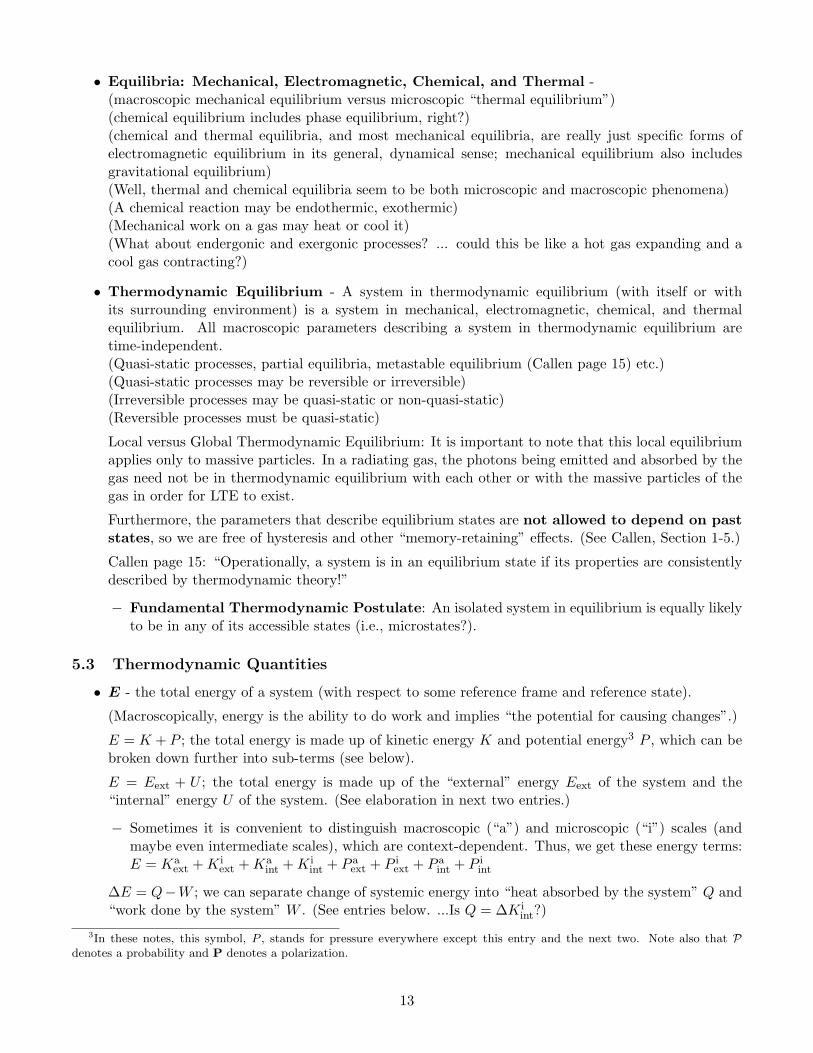
• Equilibria: Mechanical, Electromagnetic, Chemical, and Thermal -(macroscopic mechanical equilibrium versus microscopic “thermal equilibrium”)(chemical equilibrium includes phase equilibrium, right?)(chemical and thermal equilibria, and most mechanical equilibria, are really just specific forms ofelectromagnetic equilibrium in its general, dynamical sense; mechanical equilibrium also includesgravitational equilibrium)(Well, thermal and chemical equilibria seem to be both microscopic and macroscopic phenomena)(A chemical reaction may be endothermic, exothermic)(Mechanical work on a gas may heat or cool it)(What about endergonic and exergonic processes? ... could this be like a hot gas expanding and acool gas contracting?)

• Thermodynamic Equilibrium - A system in thermodynamic equilibrium (with itself or withits surrounding environment) is a system in mechanical, electromagnetic, chemical, and thermalequilibrium. All macroscopic parameters describing a system in thermodynamic equilibrium aretime-independent.(Quasi-static processes, partial equilibria, metastable equilibrium (Callen page 15) etc.)(Quasi-static processes may be reversible or irreversible)(Irreversible processes may be quasi-static or non-quasi-static)(Reversible processes must be quasi-static)

Local versus Global Thermodynamic Equilibrium: It is important to note that this local equilibriumapplies only to massive particles. In a radiating gas, the photons being emitted and absorbed by thegas need not be in thermodynamic equilibrium with each other or with the massive particles of thegas in order for LTE to exist.

Furthermore, the parameters that describe equilibrium states are not allowed to depend on paststates, so we are free of hysteresis and other “memory-retaining” effects. (See Callen, Section 1-5.)

Callen page 15: “Operationally, a system is in an equilibrium state if its properties are consistentlydescribed by thermodynamic theory!”

− Fundamental Thermodynamic Postulate: An isolated system in equilibrium is equally likelyto be in any of its accessible states (i.e., microstates?).

5.3 Thermodynamic Quantities

• E - the total energy of a system (with respect to some reference frame and reference state).

(Macroscopically, energy is the ability to do work and implies “the potential for causing changes”.)

E = K + P ; the total energy is made up of kinetic energy K and potential energy3 P , which can bebroken down further into sub-terms (see below).

E = Eext + U ; the total energy is made up of the “external” energy Eext of the system and the“internal” energy U of the system. (See elaboration in next two entries.)

− Sometimes it is convenient to distinguish macroscopic (“a”) and microscopic (“i”) scales (andmaybe even intermediate scales), which are context-dependent. Thus, we get these energy terms:E = Ka

ext +K iext +Ka

int +K iint + P a

ext + P iext + P a

int + P iint

∆E = Q−W ; we can separate change of systemic energy into “heat absorbed by the system” Q and“work done by the system” W . (See entries below. ...Is Q = ∆K i

int?)

3In these notes, this symbol, P , stands for pressure everywhere except this entry and the next two. Note also that Pdenotes a probability and P denotes a polarization.

13

− dE = dQ− dW ;− A fairly general expression of change in energy is

dE = TdS ∓ ghMi dni + V σjk dεjk ∓ φ` dQ` + VEe · dD + VHm ·dB + µm dNm + µn dNcn,summing over repeated indices. (See below for explanation of terms.)

Electromagnetic energy (I think this is sometimes called “pure” energy by popularizers of physics,since it’s energy that is not associated with matter/mass, but I would discourage this.), (the energyassociated with electromagnetic radiation is called radiant energy)

• Eext - the external energy of a system is the energy that would disappear if one moved to the restframe of the system and caused all objects outside of the system to cease to exist.

Eext = Kext + Pext; “external” kinetic Kext and “external” potential Pext energies of the system.Eext = Ka

ext +K iext + P a

ext + P iext; a⇒ macroscopic, i⇒ micro.

• U - the internal energy of a system (always in the rest frame of the system) is the energy that wouldremain if one moved to the rest frame of the system and caused all objects outside of the system tocease to exist.

U = Kint + Pint; “internal” kinetic Kint and “internal” potential Pint energies of the system.U = Ka

int +K iint + P a

int + P iint; a⇒ macroscopic, i⇒ micro.

K iint, the microscopic internal kinetic energy, may also be called the “heat energy” (Some may say

this is not proper use of the word “heat”, but it seems to be used commonly even in physics courses.In this term, the word “heat” does not imply microscopic work as it does in other contexts.)

U(S, V,N1, N2, ...) or U(other complete set of variables)(Internal energies: both macroscopic energies from visible “ordered” states os macroscopic compo-nents and microscopic energies from random, disordered motions and configurations of the particles)(Microscopic energies: translational kinetic energy, vibrational and rotational kinetic energy, andpotential energy from intermolecular forces)(Thermal energy: microscopic kinetic energies? and potential energies?)(?: Wikipedia - “Thermal energy is the internal energy of a thermodynamic system at equilibrium.The flow of thermal energy from one system to another is called heat. Thermal energy is a measureof the total vibrational energy in all the molecules and atoms in a certain substance. Thermal energyis composed of both kinetic and potential energy. The kinetic energy is from the random motion ofthe particles, and the potential energy originates from the repulsive electromagnetic force betweenthe electrons of atoms that are close to each other.”)Can derive: U = TS − PV + µN (TS: “(stored) thermal energy”; −PV “(stored) compressiveenergy”)

• W - the macroscopic mechanical work done by the system of interest.(Should this be called “generalized work” or can it all really be derived from Newtonian work, witha force acting over a distance?)(We are usually outside of the system, looking at it and saying, “What (work) are you doing forme?”)“Macroscopic work” means that there must be a change in external parameters.Each work term is a product of a generalized force Pk and its conjugate generalized displacementdX: dW =

∑k Pk dXk

(Is it appropriate to consider Pk a generalized force “on the environment due to the system” anddXk the conjugate displacement “of the (external) environment”?)

Mechanical Work

14

– (±?)V∑

ij σij dεij : stress-strain work(?); work done by viscous fluids, or plastic and/orelastic solids, where σ is the stress tensor and ε is the strain tensor. (I think σ is the generalizedforce and V dε is the conjugate displacement.) This extends also to −Γdl, the elastic work tochange the length of a wire with tension Γ by dl, and −γ dA, the surface work to change thearea of a membrane of surface tension γ by dA.

∗ P dV : pressure-volume work or “PV work”; work done by a non-viscous fluid at pressureP through a change in volume dV , where P is the generalized force and V is the generalizeddisplacement(Note that that pressure acts to expand, while tension acts to contract... if explainedcorrectly, this should make the signs obvious.)Include partial pressure here

– (±?)ψ dm: gravitational work; the work done in opposition to gravity (not in changingheight but changing mass?). ψ dm = (gh) d(

∑iMini) =

∑i ghMidni (from Alberty [5])

Chemical Work

– µdN : (heat?)If µ dN were heat, then it would be included in dQ = T dS, but that does not seem to be thecase.µ - Chemical potential or Electrochemical potential: the generalized force for the generalizeddisplacement of number of molecules (given that Ni refers to the number of “x” molecules, theunits of µi are Joules per “x” molecule.)Sometimes the “chemical potential” is defined to be the electrochemical potential µ minus themolar electrostatic energy.

∗∑

i µi dNi: chemical work (without reactions), where Ni is the number of particles of theith species∗∑

i µi dNci: chemical work (with reactions), where Nci is the number of particles of the ithcomponent in the reaction(s)

Electromagnetic Work

– (±?)∑

i Φi dQi: work done by gaining a particle of the ith species (with charge Qi in an electricpotential Φi) (charge transfer)

– −Ee ·dp: work done by a change in electric dipole moment p in an electric field Ee

−VEe · dD = −V (ε0Ee ·dEe + Ee ·dP) = −V d( ε02 |Ee|2)− (Ee ·dp)= dWe + dWpolarization

– −µ0Hm · dm: work done by a change in magnetic dipole moment m in a magnetic field µ0H−VHm ·dB = −V (µ0Hm ·dH + µ0Hm · dM) = −V d(µ0

2 |Hm|2)− (µ0Hm ·dm)= dWm + dWmagnetization

(What about V dP , Ndµ, etc?, Gibbs-Duhem relation)We will also add TdS to this formalism, but it is the heat term rather than a work term.

In (fair) generality, summing over repeated indices,dW = ±ghMi dni − V σjk dεjk ± φ` dQ` − VEe ·dD− VHm · dB− µm dNm − µn dNcn

• ∆xE - the change in mean energy calculable from the change of external parameters (i.e., due tomacroscopic work done on a system)

• Q - the “heat absorbed by a system”; −Q is the “heat given off” by the system

Q ≡ ∆E +W or Q = ∆E +W

Heat as energy exchange, definitions:

15

− Heat is the defined as the transfer of energy to a body that does not involve work–or those transfersof energy that occur only because of a difference in temperature. (from http://pruffle.mit.edu/3.00/Lecture_06_web/node2.html)

− Here, Q is simply defined to be the change in mean energy of the system not due to a change inthe external parameters. It measures the change in energy due to “purely thermal” interactions.(However, this view, which is taken from Reif (pg 73 etc), implies that µdN is a heat term inaddition to TdS, or does it? If we weigh the sample, then N could possibly be an externalparameter, no? Or would we have to know what particles are involved and their masses to dothat... and what about combinations of different particles with different masses?)

− “An energy transfer via the hidden atomic modes is called heat.” (Callen pg 8)

The word “heat” may refer to

− v. to increase the temperature of− n. “thermal energy” or “heat energy”− n. the average kinetic energy of a body (which is a state variable, and a body has heat in this

usage)− n. “heat... is the random motion of molecules” (from The Mechanical Universe: the gyroscope

episode)− n. electromagnetic radiation (esp. infrared (since humans and other everyday objects absorb it

so well?) (other frequencies?)) (as in “I feel the heat from the lamp”)− n. an environment that has the capacity to heat a body (as in “stepping out into the heat” ≈

“stepping out into the hot air”)

Talk about “latent heat” and methods of “heat transfer/flow” (redundant?) (heat as average kineticenergy versus heat as abstract energy transfer)

“heat reservoir” or “thermal reservoir” or “heat bath” (perhaps goes with the statistical materialbelow, since they have enormous “degrees of freedom”)

Thermal radiation (electromagnetic radiation emitted from the surface of an object which is dueto the object’s temperature)

• S - Entropy... different definitionsS ≡ k ln Ω(E) or S ≡ k ln

(ω(E)

[ω(E)]

)or S ≡ k lnω(E) (if only differences matter, then perhaps we

should only define differences...)S(E ± δE) ≡ k ln Ω(E, δE) = k ln(ω(E)2δE) = k ln

(ω(E)

[ω(E)]

)+ k ln

(2δE)[δE]

)≈ k ln

(ω(E)

[ω(E)]

)“information function” is the same as the reduced entropic function in thermodynamics.(What about the measurability of S?)

Callen Postulates:

1. There exist particular states (called equilibrium states) of simple systems that, macroscopically,are characterized completely by the internal energy U , the volume V , and the mole numbersN1, N2, ..., Nr of the chemical components.

2. There exists a function (called the entropy S) of the extensive parameters of any compositesystem, defined for all equilibrium states and having the following property: The values assumedby the extensive parameters in the absence of an internal constraint are those that maximizethe entropy over the manifold of constrained equilibrium states.

3. The entropy of a composite system is additive over the constituent subsystems. The entropy iscontinuous and differentiable and is a monotonically increasing function of the energy.

16

4. The entropy of any system vanishes in the state for which (∂U/∂S)V,N1,N2,...,Nr = 0 (that is, atthe zero of temperature).

Entropy may be introduced using the Claussius theorem (1854):∮

dQ/T ≤ 0 in a cyclic process(equality holding for reversible processes).

Measuring Entropy“Let’s say you pour some cold water into some hot water. What happens to the entropy? Why?”

• T , β - Absolute temperature T , Temperature parameter4 βThermodynamic definition?: “Temperature is, by definition, proportional to the average internalenergy of an equilibrated neighborhood.” (From Wikipedia Thermodynamic Equilibrium entry)From Goldstein [4]: “. . . by the equipartition theorem of kinetic theory, the average kinetic energy ofeach atom is given by 3

2kT , . . . a relation that in effect is the definition of temperature.”Statistical definition: β ≡ ∂ lnω

∂E , T ≡ 1kβ

More detail: β =∂ lnω′

∂E′

∣∣∣∣E′=Etot

where ω′ is for the heat reservoir of energy E′ that the system of

interest is in contact with, and the total energy of the two systems is Etot

• Thermodynamic Potentials - (aka auxiliary energy functions, thermodynamic free energies, freeenergy functionals); the total amount of energy in a physical system which can be converted to dowork. Legendre transforms of U .

– F ≡ U [T ] - Helmholtz free energy (sometimes A); the amount of thermodynamic energy whichcan be converted into work at constant temperature and volume. In chemistry, this quantityis called work content. (or is it just the “measures the ‘useful’ work obtainable”? Wikipedialookup)F ≡ U − TS dF (T, V ) = −SdT − PdV

– H ≡ U [P ] - Enthalpy or heat content/function; for a simple system, with a constant number ofparticles, the difference in enthalpy is the maximum amount of thermal energy derivable froma thermodynamic process in which the pressure is held constant. Also, colloquially, enthalpy isthe total amount of energy one needs to provide to create the system and then place it in theatmosphere:H ≡ U + PV dH(S, P ) = TdS + V dP

– G ≡ U [T, P ] - Gibbs free energy; the amount of thermodynamic energy in a fluid system whichcan be converted into work at constant temperature and pressure. This is the most relevantstate function for chemical reactions in open containers. (Wikipedia lookup)G ≡ U − TS + PV dG(T, P ) = −SdT + V dP

– U [T, µ] - Grand Canonical Potential...

• Massieu Functions - Legendre transforms of S.

5.4 Statistical Mechanics Terms

• Φ(E) - the number of states with energy less than E.There must, of course, be a ground state if this quantity is to be finite.(Φ(E;Xi), Φ(Xi;Xj))

4“thermodynamic beta” as opposed to the “relativistic beta”

17

• Ω(E) - the number of states with energy in the interval [E,E + δE) (or (E,E + δE)?). (Actually, afunction of E and the external parameters of the system.)This definition of Ω(E) depends on the selection of the interval δE. The magnitude of δE determinesthe precision within which one chooses to measure the energy of the system. (How does that relateto δE?) We assume that Ω(E) is an approximately smooth function, that Ω(E)→ 0 as δE → 0, andthat Ω(E) is expressible as a Taylor series in powers of δE; while δE is large compared to the spacingbetween the possible energy levels of the system, it is macroscopically small enough for the relationΩ(E) = ω(E)δE to be approximately true, where the higher order Taylor terms are neglibible andω(E) is a smooth function.

• Ω(E; yk) - the number of states with energy in the interval [E,E + δE) (or (E,E + δE)?), andparameter y with the value yk (or quantum state yk)?.

• ρ - Density of States (the number of states per some quantity)The density may be an energy-density, momentum-density, wavevector-density, etc.:ρ(E), ρ(ε), ρ(p), ρ(k), ρ(n), etc.ω(E) - the density of states (Ω(E)/δE as δE → 0).ω(Yi); the variables Yi are not necessarily external (See Reif pg 88)Variously written as ω(E), n(E), ρ(E) (or ω(ε), n(ε), ρ(ε))Note that “density of states” may refer to a function of parameters other than energy:(ω is preferrable to Ω with respect to precision of mathematical argument. Ω seems to be thetraditional choice and simplifies unit issues.)Unless there is some bound on the energy of the states,

∫∞−∞ ω(E) dE is undefined∫∞

−∞ ω(E) e−βE dE = 1

• f - Occupancyf(ε) dε: This is the average number (or number volume-density) of particles that occupy quantumstates with energy between ε and ε+ dε, right?

− nr - the number of particles (in an ensemble element system) that are in a particle quantum statelabeled by rnr = − 1

β∂ lnZ∂εr

• w - Probability Energy-Density (probability per increment of energy)

– ρ(q, p) - the “distribution function” (i.e., the probability density function of states in phasespace, a.k.a. statistical distribution function)dw = ρ(qi, pi) dq dp

– dw - the infinitesimal probability that a (sub)system occupies a state within the infinitesimal(i.e., macroscopically tiny) region between qi, pi, and qi + dqi, pi + dpi, with volume V = dq dp.

– w - the probability that a (sub)system, when observed at an arbitrary instant, will be foundin a state within the region in phase space between qi, pi, and qi + ∆qi, pi + ∆pi, with volumeV = ∆q∆p. (perhaps call it wV )(w(E) =

∫dw(E) =

∫ρ(qi, pi) dq dp

)?

w = limT→∞∆tT , where ∆t is the time spent in the specified region in phase space and T is...

the total time that the (sub)system spends in any region of phase space?I don’t see how it can really refer to a subsystem because then it would not have anything to dowith some of the qi and pi; it would be independent of some of them (so maybe it would havea Dirac delta associated with those?)

–∫∞−∞w(E) dE =

∫∞Emin

w(E) dE = 1 =∫∞−∞ ω(E) e−βEdE

18

• P - probabilityThe caligraphic P is used to avoid confusion with pressure P , polarization P, and potential energyP.

• Statistical Ensemble - Mostly, we’re interested in (or can only measure) mean quantities (meanwith respect to (local?) space and time). We use a statistical approach and model the actualsystem using an ensemble of systems, one system for each of the physically possible distinguishableconfigurations of the actual system that obey the given constraints. (According to the postulate...equiprobability...) (stationary ensemble) (mathematicians prefer “probability space”)

– Microcanonical ensemble () - an ensemble of systems, each of which is required to havethe same total energy (i.e. thermally isolated?) (Each system is isolated and in equilibrium).Ω(U, V,N) = eβTS (?)

– Canonical ensemble (Isothermal-Isochoric) - an ensemble of systems, each of which can shareits energy with a large heat reservoir or heat bath. The system is allowed to exchange energywith the reservoir, and the heat capacity of the reservoir is assumed to be so large as to maintaina fixed temperature for the coupled system. Z(T, V,N) = e−βA, ζ (?)Z =

∑i e−βEi = e−βF

– Grand Canonical ensemble - an ensemble of systems, each of which is again in thermalcontact with a reservoir. But now in addition to energy, there is also exchange of particles. Thetemperature is still assumed to be fixed. Ξ(T, V, µ) = eβPV (?)

– Isothermal-Isobaric ensemble - an “ensemble where the system is allowed to exchange energywith a heat bath of temperature T and the volume can also change though its mean value istuned by the pressure P applied. It is also called the (T,P,N)-ensemble, as the third quantitykept constant is the number of particles N. This ensemble plays an important role in chemistryas chemical reactions are usually carried out under constant pressure condition. The partitionfunction is given as ∆(N,T, P ) =

∫ ∑i exp−β(Ei + PV )dV . The characteristic state function

of this ensemble is the Gibbs free energy since ∆ = e−βG.”

– Isoenthalpic-Isobaric ensemble - (S,P ,?)

• Partition Functions - (“Boltzmann sum over states” or “sum over levels with degeneracy/multiplicity”)(functions that are sums, the partition function “encodes the underlying physical structure of thesystem”(?) or “encodes the statistical properties of a system in thermodynamic equilibrium”(?))(LOOK UP partition function, canonical ensemble, and Fermi energy on WIKIPEDIA)

− Types

∗ (Microcanonical partition function?)∗ Z - (Canonical) partition functionZ ≡

∑r e−βEr , Z = ζN

N !

in the classical approx. Z =∫· · ·∫e−β E(q1,...,pf ) dq1···dpf

h0f

∗ ζ - (individual particle, or subsystem?) (canonical?) partition functionζ ≡

∑r e−βεr (?)

ζ = Vh0

3

∫∞−∞ e

−βp2/2md3p (7.2.5) for noninteracting gas in

∗ Z - a Grand (Canonical) partition functionZ ≡

∑N Z(N)e−αN (From Reif pg 347)

∗ Ξ - Grand Canonical partition function(al?) (From ThermoPotentials paper)(What are the arguments of the partition function? If it ever takes a function as an argumentthen it may be considered properly as a functional if it returns a constant (but I don’t think

19

it does). Whether a quantity is considered an element of the complete set of parametersdetermines whether it is a mere parameter or a function...)∗ ∆ - Isothermal-Isobaric partition function∗ Q - Canonical Ensemble partition function∗ Integral Forms and the “Density of States”!!! (Planck’s constant, multidimensional forms, and

“geometric factor”)

− Properties

∗ Energy is arbitrary up to additive constant ε0, so Z ′ =∑

r e−β(Er+ε0) = e−βε0Z

lnZ ′ = lnZ − βε0 and E′ = −∂ lnZ′

∂β = −∂ lnZ∂β + ε0 = E + ε0

but entropy and all expressions for generalized forces (all eqns of state) are unchanged.∗ Z3 = Z1Z2 for a system (of degrees of freedom) made of two weakly interacting subsystems

(of dof) with partition functions Z1 and Z2. (E.g., in a diatomic gas Z1 could refer to dofof translational motion of centers of mass, and Z2 could refer to dof of rotation of moleculesabout their centers of mass.)

• Boltzmann Factor - e−βE , aka “canonical weighting factor”5

Z ≡∑

r e−βEr = e−βF (!)

∆ = e−βG (!)Pr = Ce−βEr = 1

Z e−βEr

Valid for an ensemble of systems in contact w/ a reservoirAssociated with Canonical Ensembles or Distributions(How universal is it?)

• y - the mean value of the parameter y at equilibriumy =

∑k yk P(yk) =

Pk yk Ω(E;yk)

Ω(E)

y =∑

r yk Pr = C∑

r yr e−βEr = 1

Z

∑r yr e

−βEr

y =

• Statistical Frameworks / Models for Ideal Gases -

– MB Maxwell-Boltzmann Statisticsnr =

N

Ze−βεr ;

the “Maxwell-Boltzmann distribution”

– FD Fermi-Dirac Statisticsnr =

1eα+βεr + 1

;

the “Fermi-Dirac distribution”

nr =1

eβ(εr−µ) + 1, where µ ≡ −α

β = −kTα is called the “Fermi energy” of the system

(µ is also the chemical potential)

– BE Bose-Einstein Statisticsnr =

1eα+βεr − 1

;

the “Bose-Einstein distribution”Photon statistics: nr = 1

eβεr−1; the “Planck distribution”

– Other statistics: anyon, braid, etc.5See Callen, pg 434

20

• “Fermi” Terms: Fermi level, energy, sea, function, velocity, more?“Fermi level” is the term used to describe the top of the collection of electron energy levels at absolutezero temperature. This concept comes from Fermi-Dirac statistics. Electrons are fermions and bythe Pauli exclusion principle cannot exist in identical energy states. So at absolute zero they packinto the lowest available energy states and build up a “Fermi sea” of electron energy states. TheFermi level is the surface of that sea at absolute zero where no electrons will have enough energy torise above the surface. (Relate to valence band, band gap, conduction band.)

5.5 Quantities Defined for Proofs

• Φi(ε) - the number of possible values which can be assumed by the quantum number associated withthe ith degree of freedom when it contributes to the system an amount of energy ε or less.Used in deriving the crude approximation Ω(E) ≈ Ef (Ω(U) ≈ Uf?)

• Zs(N) - ...Zs = Zs(N) = Zs(N,n) = Zs(N,n, β)Used in defining αs and then (defining/deriving) α

5.6 Comments on Terms

• Functions: There are various quantities and functions that are given names that include the word“function”, while other functions are not explicitly named as “functions”.

– “Natural function” - Callen says (pg 183) that U is a natural function of V and S (i.e., itsnatural independent variables are V and S), F is a natural function of V and T , and so on...

– “State function”

– “Partition function”

• “Relation” versus “Equation”: In thermodynamics the word relation seems to be preferred over theword equation for some reason. At the very least, this helps to distinguish between the electromag-netic Maxwell equations and the thermodynamic Maxwell relations.

5.7 More Thermodynamic Quantities

• η - Efficiency• CY - Heat capacity at constant (Y quantity name)

CY ≡(

dQdT

)Y

Specific heat“Specific heat per mole”, “Specific heat per gram”• µ Joule-Thomson Coefficient• γ Specific Heat Ratio• κ Isothermal Compressibility (or Isothermal Coefficient of Compressibility):

κ ≡ − 1V

(∂V

∂p

)T

• Bulk Modulus: the reciprocal of the isothermal compressibility

21

• Isobaric Coefficient of Thermal Expansion

1V

(∂V

∂T

)p

• α Volume Coefficient of Expansion

α ≡ 1V

(∂V

∂T

)p

• Isochoric Coefficient of Tension1p

(∂p

∂T

)V

• Fugacity (define this)y = e−u

6 Laws and Relations

CHECK HERE: http://en.wikipedia.org/wiki/Table_of_thermodynamic_equations

Some Equations

ω = ω(E, ...) Z = Z(β, ...) c= Z(T, V,N)?

lnZ = lnω − βE +: 0

ln ∆∗E

In Terms of ω In Terms of Z

E = −∂ lnω∂β E = −∂ lnZ

∂β (?)

(∆E)2 = ∂2 lnZ∂β2 = −∂E

∂β

S ≡ k lnω S = k(lnZ + βE) = k(lnZ − β ∂ lnZ∂β )

F = ... F = −kT lnZβ ≡ ∂ lnω

∂E β = ...

Pk = ... Pk = 1β∂ lnZ∂Xk

= kT ∂ lnZ∂Xk

P = ... P = kT ∂ lnZ∂V 6=

(∂E∂V

)S

(?)

cv = ... cv = kβ2 ∂2 lnZ∂β2 (?)

µj = ... µj = −kT ∂ lnZ∂Nj

α = ... α = ∂ lnZ∂N

α = −βµ (no µj?)ns = ... ns = − 1

β∂ lnZ∂εs

(∆ns)2 = − 1β∂ns∂εs

= 1β2

∂2 lnZ∂εs2

β = ∂ lnω∂E ⇔ 1

T = ∂S∂E

Pk = 1β∂ lnω∂Xk

⇔ PkT =

(∂S∂Xk

)

22

Laws of Thermodynamics

Deriving the Laws

• The Liouville equation is integral to the proof of the fluctuation theorem from which the second law ofthermodynamics can be derived.

Terse Statements

0. Zeroth Law: Thermal equilibrium is a transitive property.1. First Law: ∆U = Q−W (Heat defined or Dichotomy declared.) (Why not ∆E?)2. Second Law: a) ∆S ≥ 0 for adiabatic processes linking macrostate equilibria.

b) dS = dQT for quasi-static infinitesimal processes.

3. Third Law: S → S0 as T → 0+ for any system.

Full Statements

0. Zeroth Law

Two systems that are in thermal equilibrium with a third system are in thermal equilibrium witheach other.

1. First Law

An equilibrium macrostate of a system can be characterized by a quantity U (called “internal energy”)which has the property that, for an isolated system,

U = constant.

When the system is allowed to interact with its environment (i.e., when the system is not isolated),the resulting change in U can be written in the form

∆U = Q−W,

where W is the macroscopic work done by the system as a result of the system’s change in externalparameters. The quantity Q is the “heat absorbed by the system”.

(If Q is defined by this equation, then this is the definition of Q. If Q is defined in terms of physicalprocesses, and conservation of energy is assumed, then this is a postulate stating that there are onlytwo forms of energy exchange: work and heat.)

2. Second Law(s)

An equilibrium macrostate of a system can be characterized by a quantity S (called “entropy”),which has the properties that

(a) ∆S ≥ 0 for a thermally isolated system (i.e., for adiabatic processes) where the system goesfrom one macrostate to another,

(b) dS = dQT for a quasi-static infinitesimal process (heat reservoirs, etc.), given that the system is

not isolated and absorbs heat dQ, and where T (called “absolute temperature”) is a quantitycharacteristic of the macrotate of the system.

3. Third Law

S → S0 as T → 0+ for any system, where S0 is a constant independent of all parameters of thesystem.

23

Restatements of Thermodynamic Laws

• Allen Ginsberg:1. First: You can’t win.2. Second: You can’t break even.3. Third: You can’t quit.

• Wikipedia:0. Zeroth: If two thermodynamic systems are in thermal equilibrium with a third, they are also in

thermal equilibrium with each other.1. First: In any process, the total energy of the universe remains constant.2. Second: There is no process that, operating in a cycle, produces no other effect than the subtraction

of a positive amount of heat from a reservoir and the production of an equal amount of work.3. Third: As temperature approaches absolute zero, the entropy of a system approaches a constant.C. Combined Law: dE − TdS + PdV ≤ 0. (First + Second)

• First Law

− (1865) “The energy of the universe is constant.” –Claussius− A state function, called the internal energy, exists for any physical system–and the change in the

internal energy during any process is the sum of the work done on the system and the heat transferedto the system.

− The work done on a system during an adiabatic process is a state function and numerically equalto the change in internal energy of the system.

− Interpretations:

∗ A restriction on the processes that occur in any system.∗ A definition.∗ A bookkeeping device.

• (1865) Second (a): “The entropy of the universe tends to a maximum.” –Claussius• (1874) Thomson formally states the second law of thermodynamics• (1906) Nernst presents a formulation of the third law of thermodynamics. (The third law of thermo-

dynamics may also be called the Nernst heat theorem.)• (What about other heat laws, such as “the heat law” dS = (dE + PdV )/T ?)

Tentative Fourth Laws or Principles

Most variations of hypothetical fourth laws (or principles) have to do with the environmental sciences,biological evolution, or galactic phenomena. Most fourth law statements, however, are speculative andfar from agreed upon. The most common proposed Fourth Law is the Onsager reciprocal relations.Another example is the maximum power principle as put forward initially by biologist Alfred Lotka in his1922 article Contributions to the Energetics of Evolution.

Statistical Relations and Postulate

• S = k ln Ω

• P ∝ Ω ∝ eS/k

24

• Equal a priori probability postulate: Given an isolated system in equilibrium, it is found with equalprobability in each of its accessible microstates. (or thermodynamic postulate?)

Fundamental Relations for common Thermodynamic Potentials

(“pre-Maxwellian Relations”) (partial Legendre Transforms of E; of S ⇒ Massieu functions)

• In general, dU = −∑t

k=0 Pk dXk = TdS −∑t

k=1 Pk dXk

Or dU = −∑r,t

m=0,k=0 Pm,k dXm,k for r-component systems and t force/displacement conjugatepairs

· E = F + TS = H − PV = G+ TS − PV· F ≡ E − TS = H − TS − PV = G− PV· H ≡ E + PV = F + TS + PV = G+ TS

· G ≡ E − TS + PV = F + PV = H − TS

• dE = TdS − PdV T =(∂E∂S

)V

−P =(∂E∂V

)S

• dF = −SdT − PdV −S =(∂F∂T

)V

−P =(∂F∂V

)T

• dH = TdS + V dP T =(∂H∂S

)P

V =(∂H∂P

)S

• dG = −SdT + V dP −S =(∂G∂T

)P

V =(∂G∂P

)T

Don’t forget to list the assumptions used here!

• Hey, should the Gibbs-Duhem relation go here?

Maxwell Relations

• ∂2E∂V ∂S

= ∂2E∂S ∂V

⇒(∂T∂V

)S

= −(∂P∂S

)V

• ∂2F∂T ∂V

= ∂2F∂V ∂T

⇒ −(∂S∂V

)T

= −(∂P∂T

)V

• ∂2H∂S ∂P

= ∂2H∂P ∂S

⇒(∂T∂P

)S

=(∂V∂S

)P

• ∂2G∂T ∂P

= ∂2G∂P ∂T

⇒ −(∂S∂P

)T

=(∂V∂T

)P

Further Relations Derived from Maxwell Relations

• The Granddaddy of Relations:(∂U∂V

)T

= T(∂P∂T

)V− P (Why did Putterman call it that?)

• Fluctuations from equilibrium:Say a variable y is fluctuating about the equil value y. Given that P(y)

Pmax= e(S(y)−Smax)/kB , using

a Taylor expansion of S(y) about S(y) = Smax, and assuming the third- and higher-order partial-derivative-of-S-wrt-y terms are negligible, we find that the fluctuations are described by a Gaussiandistribution with dispersion ⟨

(y − y)2⟩

= kB

∣∣∣∂2S/∂y2 (y)∣∣∣−1

25

More Fundamental Relations

Gibb’s free energy G; “this is the thermodynamic potential that depends on magnetization M and tem-perature T” (Peskin pg 269) H is the external magnetic field.(

∂G

∂M

)T

= H

7 People and Old Eponymous Laws

See http://en.wikipedia.org/wiki/Scientific_laws_named_after_people

• Antoine-Laurent de Lavoisier, Nicolas Leonard Sadi Carnot, Robert Boyle, Jacques Charles, JosephLouis Gay-Lussac, John Dalton, Amedeo Avagadro, Benoit Paul Emile Clapyron, Rudolf Claussius,Josiah Willard Gibbs, Pierre Duhem, Henri-Louis Le Chatelier• Lavoisier• (1662) Boyle’s Law

PV = const.

• (1787) Charles’s Law or Law of Charles and Gay-Lussac

V

T= const. or

V1

T1=V2

T2

• (1801) Dalton’s Law of Partial Pressures

Ptotal =n∑i=1

pi

...related to ideal gas law...• Gay-Lussac’s Law(s)

1. (1802) The pressure of a fixed amount of gas at fixed volume is directly proportional to its temper-ature in kelvins:

P

T= const. or

P1

T1=P2

T2

for the same substance under two different sets of conditions (P1, T1) and (P2, T2).2. (1809) The ratio between the combining volumes of gases and the product, if gaseous, can be

expressed in small whole numbers.

• (date?) Combined Gas Law (⇐ Gay-Lussac [1] + Charles’s + Boyle’s Laws)

PV

T= const. or

P1 V1

T1=P2 V2

T2

• (1811) Avagadro’s LawEqual volumes of gases, at the same temperature and pressure, contain the same number of particlesor molecules:

V

N= a or

V (T, P )N

= a(T, P )?

where V is the volume of any gas at a particular temperature T and pressure P , N is the number of

26

particles or molecules, and a is a contant (that depends on the temperature and pressure?)Thus, the number of molecules in a specific volume of gas is independent of the size or mass of the gasmolecules.The most important consequence of Avogadro’s law is the following: The ideal gas constant has thesame value for all gases. This means that the constant:

P1 V1

T1 n1=P2 V2

T2 n2= const.

• (1834) Ideal Gas Law (⇐ Combined Gas + Avagadro’s Laws) (Emile Clapyron)The equation of state of a hypothetical ideal gas. PVm = R[TC + (273.15 C)]

PV = nRT

• (1843) Carnot’s Principle: (Carnot cycle, Claussius Theorem?) Clapeyron made a definitive state-ment of Carnot’s principle, what is now known as the second law of thermodynamics.• (1888) Le Chatelier’s Principle (?): the response of a chemical system perturbed from equilibrium

will be to counteract the perturbation.• Claussius-Claypeyron Relation

The Clausius-Clapeyron relation gives the slope of the coexistence curve (the line separating two phasesin a P -T diagram) and characterizes phase transitions:

dPdT

=L

T∆V

where L is the latent heat.Derivation: use chemical potentials, Gibbs-Duhem relation, and the second law (b).• Others: (1880) Amagat’s Law of Partial Volumes, Raoult’s Law and Henry’s Law (re: partial vapor

pressures of ideal solutions and concentrations of solute)

8 Theorems, Postulates, Hypotheses, and Demons

• Fundamental Thermodynamic Postulate: An isolated system in equilibrium is equally likely tobe in any of its accessible states. (or statistical postulate?)

• Liouville Theorem and Equation (from classical mechanics)Applies to quasi-closed subsystems and is thus only valid for not-too long intervals of time, duringwhich the subsystem behaves as if closed, to a sufficient approximation. The distribution function isconstant along the phase trajectories of the sybsystem. (Landau pg 10)A consequence of Liouville’s theorem: “if one considers a representative ensemble of ... isolatedsystems where these systems are distributed uniformly (i.e., with equal probability) over all theiraccessible states at any one time, then they will remain uniformly distributed over these statesforever.” (Reif pg 54)

• Fluctuation TheoremThe Liouville equation is integral to the proof of the fluctuation theorem from which the second lawof thermodynamics can be derived.

• Claussius Theorem (Carnot cycle, Carnot princple?)

27

• Lemma: Any reversible process can be replaced by a combination of reversible isothermal and adia-batic processes.

• Helmholtz Theorem (of classical mechanics)

• Ergodic Hypothesis

• Generalized Helmholtz TheoremA multidimensional version of the Helmholtz theorem, based on the ergodic theorem of George DavidBirkhoff.

• (1872) H-Theorem (regarding entropy) and the approach to equilibrium(1876) Loschmidt’s paradoxQuantum mechanical H-theorem1872 - Ludwig Boltzmann states the Boltzmann equation for the temporal development of distributionfunctions in phase space, and publishes his H-theorem1876 - Johann Loschmidt criticises Boltzmann’s H theorem as being incompatible with microscopicreversibility (Loschmidt’s paradox).

• Equipartition Theorem (classical statistical mechanics)

• Euler’s Theorem for homogeneous functions

• Nernst Postulate

• Gibbs Phase Rulei, Number of independent intensive variables (Number of degrees of freedom f = i) (really?); s,Number of chemical species; p, Number of phases; r, Number of independent reactions; c, Numberof components (c = n− r)i = s− r − p+ 2 = c− p+ 2 if chemical reactions are involved

i = s−p+2 The Gibbs-Duhem equation can be regarded as the source of the phase rule, for a systeminvolving only PV work and chemical work, but no chemical reactions.

i = s+ 1 for a one-phase system

• Natural Variables, number of potentials, etc.v, Number of natural variables (independent variables to describe the extensive state); f Number ofdegrees of freedom (f = i)

v = i+ p = s− r + 2 = c+ 2 for a system with chemical reactionsv = i+ p = s+ 2 for a system without chemical reactions

2v − 1, Number of Legendre transforms (non-zero ones?)

2v, Number of thermodynamic potentials for a system(2v includes the potential that is equal to zero and yields the Gibbs-Duhem equation)

v(v − 1)/2, Number of Maxwell equations for each of the thermodynamic potentials

[v(v − 1)/2]2v, Number of Maxwell equations for all of the thermodynamic potentials for a system

When Legendre transforms are used to introduce two new natural variables (T, P ), then 2v = 22 = 4thermodynamic potentials are related by Legendre transforms, as we have seen with U , H, A, andG. There are four Maxwell equations.

Intensive variables are introduced as natural variables only by use of Legendre transforms. Since aLegendre transform defines a new thermodynamic potential, it is important that the new thermo-dynamic property have its own symbol and name. The new thermodynamic potentials contain all

28

the information in U(S, V ni), and so the use of U , H, A, G, or other thermodynamic potential inplace of U is simply a matter of convenience.

• Maxwell’s Demon

• Laplace’s Demon

8.1 Proving Theorems

• Virial theorem + Equipartition theorem ⇒ Ideal Gas Law• Virial theorem + (?) ⇒ equations of state for imperfect or nonideal gases

9 Important Physical Systems, Phenomena, and Applications

• Inelastic collisionsThe importance of inelastic collisions of the first and second kinds for reaching equilibrium.

− 1st Kind: An inelastic collision in which some of the kinetic energy of translational motion isconverted to internal energy of the colliding systems. A.k.a. an endoergic collision.

− 2nd Kind: An inelastic collision in which some of the internal energy of the colliding systems isconverted to kinetic energy of translation. A.k.a. an exoergic or “super-elastic” collision.

• Ideal Gas(Departure function)• Chemistry

electrochemical cell, chemical reactions, chemical thermodynamics, Nernst equation, activation energy,Arrhenius equation• Black-Body Radiation

− Some History

∗ 1791 - Pierre Prevost shows that all bodies radiate heat, no matter how hot or cold they are∗ 1804 - Sir John Leslie observes that a matte black surface radiates heat more effectively (i.e.,

loses energy more quickly due to radiation) than a polished surface, suggesting the importanceof black-body radiation∗ 1831 - Macedonio Melloni demonstrates that black-body radiation can be reflected, refracted,

and polarised in the same way as light∗ 1859 - Gustav Kirchoff shows that energy emission from a black body is a function of only

temperature and frequency (he introduces the term “black body” in 1862)∗ 1879 - Jozef Stefan observes that the total radiant flux from a black body is proportional to the

fourth power of its temperature and states the Stefan-Boltzmann law.∗ 1884 - Boltzmann derives the Stefan-Boltzmann black-body radiant flux law from thermody-

namic and electrodynamic considerations.∗ 1893 - Wilhelm Wien discovers the displacement law for a blackbody’s maximum specific inten-

sity.

− Energy emission from a black body is a function of only temperature and frequency (and emissionangle, since a black body is a Lambertian radiator).

− perfect absorber and “perfect emitter” (I think black-bodies are defined to be “perfect” emitters,because their emission spectra are mathematical envelopes for all other emission by bodies: they

29

have an emissivity of ε = 1)− emissivity: ratio of energy radiated by the material to energy radiated by a black body at the same

temperature. (specific emissivity? depends on temperature, frequency/wavelength, emission angle)− absorptivity− All bodies radiate, whatever their temperature. Kirchhoff’s Law of thermal radiation: At

thermal equilibrium, emissivity equals absorptivity for all bodies.− Grey body, brown body

• EnginesCarnot Cycle• Superconductivity• Magnetic cooling• Bose-Einstein condensate• Fermion condensate (Advanced?)• (Reif Ch 12,13: scattering, thermal conductivity, electrical conductivity, viscosity)• Solar Spectrum: absorption lines and other deviations from the black-body spectrum (why should it

emit like a black body in the first place?)

− Inelastic collisions of the second kind− Thermal doppler shifting− Bremsstrahlung radiation from collisions− Surface of last scattering for different frequencies is at different elevations and temperatures− The “wings ” on the absorption line (or dip) are caused by uncertainty in the energy (frequency) of

the photons, since they are released by atoms and molecules that only briefly occupy excited states

• Joule-Thomson process / effect / (expansion?) (Throttling) (or Joule-Kelvin)the change in temperature that accompanies expansion of a gas without production of work or transferof heat. At ordinary temperatures and pressures, all real gases except hydrogen and helium cool uponsuch expansion; this phenomenon often is utilized in liquefying gases• Joule expansion• Entropy of a gravitationally collapsing gas (Seemingly defies 2nd law of thermo)

See http://math.ucr.edu/home/baez/entropy.html

10 Models, Paradoxes, and Catastrophes

• Ideal Gas

• van der Waals Gas

• Molecular gasline Virial Expansion of the equation of statepkT = n+B2(T )n2 +B(T )n3 + · · ·Virial coefficients: B1(T ) = 1, B2(T ), B3(T ), ...B2(T ) = −2π

∫∞0 (e−βu − 1)R2 dR where u is the intermolecular potential

• Black-body RadiationRadiation of a black-body in thermal equilibrium.

30

Black-body energy flux density (or intensity, power area-density, radiant flux, emissive power, ir-radiance), in terms of intensity frequency-solid-angle-density and intensity wavelength-solid-angle-density:

s = I =∫i(ν, T ) dν dΩ =

∫i(λ, T ) dλ dΩ

“Energy density distribution”: u(ν, T ) (see if the equations using this below are in a good unitsystem)

− (1879) Stefan-Boltzmann Law (a.k.a. Stefan’s Law)Black-body energy flux density:

s = ε σT 4

where ε is the black-body’s emissivity (ε = 1 for a perfect black-body) and the Stefan-Boltzmannconstant (or Stefan’s constant) σ = (5.670 400×10−8 Wm−2K−4). Using Planck’s Law, one canderive that σ = 2π5k4/15c2h3. (σ = 8π5k4/15h3c3?)The law was discovered experimentally by Jozev Stefan in 1879. The proportionality was derivedtheoretically, using thermodynamics and Maxwell’s electrodynamics, by Ludwig Boltzmann in1884. (Or was the law, including the proportionality, derived in 1884?)

− (1893) Wien’s Displacement Law

λpeak =b

Tor νpeak =

c

λpeak=

4.96hkT

where Wien’s displacement contant b = (2.897 768 5(51)×10−3 m ·K). (Using Planck’s Law, onecan derive that b = hc/kx where x is the solution to x/(1 − e−x) = 5: x = 4.965 114 231 744 . . .)(x = 4.9663?)Wien formulated his law based on empirical data.

− (1894) Wien’s Distribution Law (a.k.a. Wien’s Approximation) (1894 or 1896?)Energy density distribution:

u(ν, T ) = Aν3e−γν/T

where A and γ are two parameters that can be adjusted to fit experimental data.Wien derived this using the Stefan-Boltzmann law and thermodynamical arguments.

i(ν, T ) =2hν3

c2e−hν/kT or i(λ, T ) =

2hc2

λ5e−hc/λkT (?)

− (1900) Rayleigh-Jeans LawEnergy density:

f(λ, T ) = 8πkT

λ4(1905)

f(λ, T ) ∝ T

λ4(1900)

u(ν, T ) =8πν2

c3kT

Derived using thermodynamics and electrodynamics by Rayleigh in 1900 with these steps: assumethe radiation exists in standing E&M waves, then the energy density is the product of the number

31

of modes of oscillation per unit volume per unit frequency and the average energy per mode (whichis independent of frequency)

u(ν, T ) = N(ν) 〈E〉 =8πν2

c3

∫∞0 E e−E/kTdE∫∞

0 e−E/kTdE=

8πν2

c3kT,

by the equipartition theorem.(Lord Rayleigh derived the proportionality relation in 1900, while Sir James Jeans derived theproportionality constant in 1905.)

− (1901) Planck’s Law of black-body radiation (a.k.a. Wien-Planck Law)

u(ν, T ) =8πν2

c3

hν

ehν/kT − 1

Planck’s quantization rule, or postulate, was that the energy emitted by the oscillating charges inthe wall of the cavity must be integer multiples of hν (E = nhν) so the average energy per modeor oscillator must be a sum rather than an integral:

〈E〉 =∑∞

n=0 nhν e−nhν/kT∑∞

n=0 e−nhν/kT =

hν

ehν/kT − 1

which is independent of frequency.

i(ν, T ) =2hν3

c2

1ehν/kT − 1

or i(λ, T ) =2hc2

λ5

1ehc/λkT − 1

(?)

f(λ, T ) =8πhcλ5

1ehc/λkT − 1

• Ultraviolet Catastrophe (or Rayleigh-Jeans Catastrophe)Term “UV catastrophe” coined in 1911 by Paul Ehrenfest. (Ultraviolet is merely referring to highfrequency electromagnetic radiation, which includes x-rays, gamma rays, and the whole upper spec-trum. On an intensity-frequency plot, there is no spike or divergence within the UV window of thespectrum; however, on an intensity-wavelength plot, the curve diverges as wavelength vanishes.)(energy density diverges or goes to infinity as frequency goes to infinity, and thus total energy di-verges)Planck did not consider the equipartion theorem to be universally valid, so he never noticed any sortof “catastrophe” - it was only discovered some five years later by Einstein, Lord Rayleigh, and SirJames Jeans.

• Specific Heat (or specific heat capacity) of Solid Bodies and Gases1819 - Pierre Louis Dulong and Alexis Therese Petit give the Dulong-Petit law for the specific heatcapacity of a crystal“As far as the specific heat of solid bodies is concerned, Einstein’s theory, which rested upon theassumption of a single natural vibration of the atom, was extended by M. Born and Th. von Krmn tothe case of various kinds of natural vibrations, which approached more nearly to the truth. P. Debyesucceeded, by means of a bold simplification of the stipulations for the character of natural vibrations,in producing a relatively simple formula for the specific heat of solid bodies which, particularly forlow temperatures, not only satisfactorily reproduces the measurements obtained by W. Nernst andhis pupils, but is also compatible with the elastic and optical properties of these substances. The

32

quantum of action also comes to the fore in considering the specific heat of gases. W. Nernst hadearlier suggested that to the quantum of energy of a vibration there must also correspond a quantumof energy of a rotation, and accordingly it was to be expected that the rotational energy of the gasmolecules would disappear with falling temperature. The measurements by A. Eucken on the specificheat of hydrogen confirmed this conclusion, and if the calculations of A. Einstein and O. Stern, P.Ehrenfest and others have not until now afforded any completely satisfactory agreement, this liesunderstandably in our, as yet, incomplete knowledge of the model of a hydrogen molecule. The factthat the rotations of the gas molecules, as specified by quantum conditions, do really exist in Nature,can no longer be doubted in view of the work on absorption bands in the infrared by N. Bjerrum, E.von Bahr, H. Rubens, G. Hetmer and others, even though it has not been possible to give an all-roundexhaustive explanation of this remarkable rotation spectra up to now.” – Planck [3] 1920

− Debye model of solids, (specific) heat capacityIn 1912, Debye extended Albert Einstein’s theory of specific heat to lower temperatures by in-cluding contributions from low-frequency phonons.How much of this is important to know? ...

Debye frequency: ωD = cs

(6π2N

V

)1/2

Debye function: fD(y)Debye temperature: θDDebye approximation

CV = 12π4

5 Nk(TθD

)3

− Einstein model of solids, heat capacity

• Gibbs Paradox (→ Sackur-Tetrode equation)

• Ising Model, Potts Model, Etc.

• Mean Field TheoryBogoliubov inequalityReif pg 430: Weiss molecular-field theory, approximation, Brillouin function, (critical temperature...)Curie temperature (pg 432), (general consistency condition, pg 433)

• ...

11 Advanced or Additional Topics, (Beyond These Notes?)

• Random Processes

− Brownian motion− Langevin, Fokker-Planck equations (nonequilibrium)

• Nonequilibrium Statistical MechanicsLiouville’s Thm, Boltzmann Eqn (far from equilibrium, transport quantities) [collisionless BoltzmannEqn called Liouville Eqn or Vlasov Eqn],• Phase transitions

− (First-Order phase transition)− Second-Order phase transition (critical point), Landau theory, (QFT, field mass → 0 at phase

transition; Peskin pg 268-9)

• Boltzmann Equation

33

• 1948 - Claude Elwood Shannon establishes information theory. (information entropy here?)• 1957 - Edwin T. Jaynes gives MaxEnt interpretation of thermodynamics from information theory.• 1972 - Jacob Bekenstein suggests that black holes have an entropy proportional to their surface area.• 1974 - Stephen Hawking predicts that black holes will radiate particles with a black-body spectrum

which can cause black hole evaporation

12 Open Questions and Mysteries

• Theory of melting• Theory of the speed of sound• (Complete model for the creation of the magnetic field of the Earth?)

13 Constants and Important Quantities

Name of Constant Symbol Value

Boltzmann constant k (oftentimes written elsewhere as k or kB) 1.38×10−23 J/KElectrostatic (Coulomb) constant Ke (oftentimes written elsewhere as k or kC) 8.99×109 Nm2/C2

(universal or ideal) gas constant R 8.314 JK−1mol−1

14 Problem-Solving Issues

• When you are asked to “write down the fundamental thermodynamic relation” for a particular system,this is (or should be) different than being asked to “write down a fundamental thermodynamic relation”for that system. In the first case, you should write down the fundamental relation of thermodynamics,

dE = TdS − PdV or dE = dQ− dW ?

and then solve for and substitute the appropriate quantities (e.g., . . . , or. . . ). In the second case, youshould

References

[1] Herbert B. Callen: Thermodynamics and an Introduction to Thermostatistics, Second Edition, JohnWiley & Sons (1985)

[2] F. Reif: Fundamentals of Statistical and Thermal Physics, McGraw-Hill (1965)

[3] Max Planck: “The Genesis and Present State of Development of the Quantum Theory,” from NobelLectures, Physics 1901-1921, Elsevier Publishing Company, Amsterdam (1967). Available at <http://nobelprize.org/nobel_prizes/physics/laureates/1918/planck-lecture.html> (Accessed Jan-uary 2007).

[4] Herbert Goldstien: Classical Mechanics, Second Edition, Addison-Wesley (1980)

[5] Robert A. Alberty: “Use of Legendre Transforms in Chemical Thermodynamics,” International Unionof Pure and Applied Chemistry (IUPAC) Technical Report (Physical Chemistry Division, Commision onThermodynamics). Available at <http://www.iupac.org/publications/pac/2001/pdf/7308x1349.pdf>.

34