Notes on Linear Robust Control - Drexel...

Notes on Linear Robust

Control

MEM 633 October 2, 2002

Professor Harry G. Kwatny Office: 3-151A

[email protected] http://www.pages.drexel.edu/faculty/hgk22

mailto:[email protected]

MEM 633-634 Notes Professor Kwatny

Contents

1 Introduction to the Robust Control Problem......................................................... 1

2 State Space Models ................................................................................................... 2

2.1 Solutions of Linear Systems ............................................................................... 2

2.2 The Matrix Exponential ...................................................................................... 2

2.3 Controllability ..................................................................................................... 2

More on Invariance ..................................................................................................... 7

2.4 Observability....................................................................................................... 7

More on Invariance ..................................................................................................... 9

2.5 Kalman Decomposition ...................................................................................... 9

2.6 Thorp-Morse Form.............................................................................................. 9

2.7 Zeros ................................................................................................................... 9

3 Nominal Controller Design: State Space Perspective.......................................... 12

3.1 State Feedback .................................................................................................. 12

Pole Placement.......................................................................................................... 12

The Linear Regulator Problem.................................................................................. 12

3.2 Observers & the Separation Principle............................................................... 12

3.3 Disturbance Rejection....................................................................................... 12

4 Transfer Function Models...................................................................................... 13

4.1 State Space to Transfer Function ...................................................................... 13

4.2 Frequency Response ......................................................................................... 13

4.3 Poles & Zeros of Transfer Functions ................................................................ 13

4.4 Realizations....................................................................................................... 13

5 Closed Loop Transfer Functions ........................................................................... 15

5.1 Well Posedness ................................................................................................. 15

5.2 Closed Loop Transfer Functions....................................................................... 15

Output ....................................................................................................................... 15

Error .......................................................................................................................... 15

Control ...................................................................................................................... 15

ii


6 Performance in the Frequency Domain................................................................ 16

6.1 Sensitivity Functions......................................................................................... 16

A fundamental tradeoff ............................................................................................. 16

6.2 Sensitivity Peaks ............................................................................................... 17

6.3 Bandwidth ......................................................................................................... 17

6.4 Limits on Performance...................................................................................... 17

7 Nominal Controller Design: Frequency Domain Perspective............................. 18

7.1Equation Section 1 Full State Feedback Controllers ............................................ 18

The Quadratic Regulator Problem ............................................................................ 18

Min-Max Control ...................................................................................................... 19

Solving the Riccati Equation .................................................................................... 21

7.2 Output Feedback Controllers ............................................................................ 22

The Classical H2 Problem – LQG............................................................................ 22

The Modern Paradigm .............................................................................................. 23

Solution Summary .................................................................................................... 26

8 Robust Stability & Nyquist Analysis..................................................................... 30

8.1 SISO Nyquist Analysis ..................................................................................... 30

Guaranteed Gain and Phase Margin ......................................................................... 31

8.2 MIMO Nyquist Analysis................................................................................... 31

8.3 M ∆ - Structure.................................................................................................. 32

8.4 Small Gain Theorem......................................................................................... 32

8.5 Robust Stability of the M ∆ - Structure ............................................................ 33

9 Robust Performance ............................................................................................... 34

10 Some Complex Variable Concepts .................................................................... 35

10.1 Analytic Functions ............................................................................................ 35

Residue Theorem ...................................................................................................... 35

Poisson Integrals ....................................................................................................... 36

Bode Waterbed Formula ........................................................................................... 37

10.2 Parseval’s Theorem........................................................................................... 38

11 Normed Linear Spaces ....................................................................................... 40

iii


11.1 Norms and Normed Linear Spaces ................................................................... 40

Examples of normed linear spaces:........................................................................... 40

11.2 System Norms/ Induced Norms ........................................................................ 42

Transfer matrix norms............................................................................................... 42

iv


1 Introduction to the Robust Control Problem

1


2 State Space Models

2.1 Solutions of Linear Systems

( ) ( )x A t x B t u= +

0 0 00

( , ) ( , ) ( )t

x(t; x ,u) t t x t s B s u(s)ds= Φ + Φ∫

( , ) ( ) ( , ), ( , )d t A t t t tdt

τ τΦ = Φ Φ = I

2.2 The Matrix Exponential

Cayley-Hamilton Theorem: Every square matrix satisfies its own characteristic

equation, i.e. if

φ λ λ λ λ( ) = − = + + +−−I A a an

nn

11

0

Then

φ( )A A a A a Inn

n= + + + =−−

11

0 0

From this we obtain:

e t I t A tAtn

n= + + + −−Aα α α0 1 1

1( ) ( ) ( )

2.3 Controllability

We briefly review some basic concepts and results for linear autonomous systems

BuAxx +=

Cxy =

where . Recall that given an initial state x(0) = x0 and a control

u(t), t > 0, the corresponding trajectory is define by the variations of parameters formula

pmn RyRuRx ∈∈∈ ,,

∫+=t

A(t-s)At Bu(s)dse x e,u) x(t;x0

00

2


Definition: A state is reachable from x0 if there exists a finite time t > 0 and a piecewise continuous control u such that .

nRx ∈1

10 x,u)x(t;x =0xR denotes the set

of states reachable from x0.

Let us make a few preliminary observations.

If 1x is reachable from 0x in some time , it is reachable in every time t. To see this

simply rescale s:

1 0t >

( )

( )

111 1

1 1

1 11 1

0 0

0

stt

stt

t tA(t - )A(t -s) st st

t t

tA(t- ) A(t -t) st st

t t

e Bu(s)ds e Bu( )d

e Be u( )d

=

=

∫ ∫

∫

Thus, we have the replacement 11

( ) A(t -t) sttu s e u( )→ .

Notice that 1x is reachable from 0x if and only if 1At

0x e x− is reachable from the origin

for , viz 0 t< < ∞

1 0 1 00 0

t tAt A(t-s) At A(t-s)x e x e Bu(s)ds x e x e Bu(s)ds= + ⇔ − =∫ ∫

As a result, we focus on characterizing the set of states reachable from the origin. Let

denote the linear vector space of control functions , and U 1( ), [0, ]u tτ τ ∈ nR≅X the

space of states 1( )x t . The inner product on is the usual U

1

0ˆ ˆ, ( ) (

t Tu u u u dτ τ= ∫ ) τ

The mapping defined by :A →U X

11( )

1 0( ) ( )

t A tx t e Buτ τ τ−= ∫ d (1.1)

defines the state reached from the origin at time when the control u is applied on the

time interval [0 .

1t

1, ]t

A state 1x is reachable from the origin over the time interval [0 if and only if the

relation

1, ]t

1( )A u x= has a solution u t . Such a solution exists if and only if ( ) 1 Imx A∈ . It is

more convenient to apply the equivalent condition *1 Imx AA∈ because .

So let’s us prove this result.

* :AA →X X

3


Lemma 1: There exists a solution u of 1( )A u x= if and only if *1 Imx AA∈ .

Lemma 1

Proof: Sufficiency ( *1 1Im Imx AA x A∈ ⇒ ∈ ) is obvious. To prove necessity, assume

1 ( )x A u= and *Im1x AA Im∉ . Since *kerA A= ⊕X , 1x has a component in *ker A . It

follows that there exists an 2x such that and . Now, *2AA x 0= 1 2 0x x ≠T

* * *2 2 2 20 0Tx AA x A x A x= ⇒ = ⇒ = 0

Then

*1 2 2 2, ,Tx x Au x u A x= =

X U0=

contradicting the condition . 1 2 0Tx x ≠

Qed

To use this result, we need to calculate the adjoint mapping . It is defined by * :A →X U

*, ,x Au A x u=X U

Thus,

( )

( )

1 11

11

( )*

0 0

( )

0

( ) ( ) ( )

( )T

t tT A t sT

Tt A t tT

A x u d x e Bu s ds

B e x u t d

τ τ −

−

=

=

∫ ∫

∫ t

From this we identify

1( )* ( )TA t tTA x B e x−= (1.2)

so that

11 1( ) ( )*

0( )

Tt A t A tTAA x e BB e d xτ τ τ− − = ∫

Consequently, in view of , we have the following result.

Proposition: The set of states reachable from the origin over the time interval [0 is 1, ]t

11 1( ) ( )*

0Im Im

Tt A t A tTAA e BB e dτ τ τ− − = ∫

Definition: The matrix

11 1( ) ( )

1 0( )

Tt A t A tTCG t e BB e dτ τ τ− −= ∫

4


is called the controllability Gramian.

Definition: The system or the matrix pair (A,B) is said to be (completely) controllable if any state is reachable from any other state in finite time.

nRx ∈1nRx ∈0

Proposition: The system is completely controllable if and only if

1rank ( )CG t n=

Choose a point η ∈X and use it to construct a control 1( )*( ) ( )TA t tTu t A B eη η−= = . Starting

at , apply the control to obtain. (0) 0x =

11 1( ) ( )*

1 10( ) ( ) ( )

Tt A t A tTCx t AA e BB e d G tτ τη τ η η− − = = = ∫ (1.3)

Any 1x reachable from the origin satisfies this relation for some η . Hence, a control that

steers the system from the origin to 1x on the interval [0 is 1, ]t

1( )*( ) ( )TA t tTu t A B eη η−= = (1.4)

for any η that satisfies

1( )CG t x1η = (1.5)

If the system is completely controllable there is a unique η , yielding

(1.6) 1( ) 11 1( ) ( )

TA t tTCu t B e G t x− −=

It is interesting to note that if the system is unstable, the control at any time t becomes

small as . The opposite occurs if the system is stable. This is consistent with the

well known fact that highly maneuverable vehicles tend to be unstable or marginally

stable.

1t → ∞

Let : Im( )B=B , and

1 1| : Imn nA A A B AB A− − B = + + + = B B B B …

Then we have the following basic result

Theorem: 0R A= B . Proof: We need to show that

Im ( ), 0CA G t t= >B

5


Since is symmetric (⇒ ), this is equivalent to ( )CG t Im kerCG= ⊕X CG

ker ( ), 0CA G t⊥

= >B t

First show, ker ( )Cx G t x A⊥

∈ ⇒ ∈ B . If ker ( )Cx G t∈ , then so that 0TCx G x =

2( )

00, 0

t T A tx e B dτ τ τ− = <∫ t<

Therefore

0, 0T Asx e B s t= < <

Expanding Ase and comparing coefficients leads to

0, 0, , 1T ix A B i n= = … −

] 0

Consequently, which implies that x is orthogonal to 1[T nx B AB A B− =… A B , i.e.

x A⊥

∈ B .

Now show ker ( )Cx G t x A⊥

∈ ⇐ ∈ B . But x A⊥

∈ B

0

implies so

reversing the above steps leads to . This is true only if

1[ ]T nx B AB A B− =…

ker ( )C

0

TCx G x = x G t∈ .

Qed

Theorem: The system or the matrix pair (A,B) is (completely) controllable if and only if 0

nR R= , or equivalently nBAABB n =− ]rank[ 1…

Proof:

Qed

We wish to emphasize the geometric aspects of controllability and observability.

To do so fully requires the concept of an invariant subspace.

Definition: A subspace V is invariant with respect to A if nR⊆

VAV ⊆Clearly, every eigenvector defines a one-dimensional invariant subspace. Furthermore,

the set of all vectors satisfying h

Ah hλ=

is called the eigenspace of A associated with the eigenvalue λ . Every eigenspace of A is

an invariant subspace as is every subspace that can be constructed as the sum of

6


eigenspaces. Perhaps less obvious is the fact that every invariant subspace is the direct

sum of eigenspaces.

) is A-invariant, i.e., . In fact is the smallest A-invariant

subspace of

0(R )0()0( RAR ⊆ )0(RnR containing B. Moreover, if there exists a system of

coordinates in which the state equations take the form:

1) n=0(dim R

xx

A AA

xx

Bu1

2

11 12

22

1

2

1

0 0LNMOQP =LNM

OQPLNMOQP +LNMOQP , x1∈Rn1 , x2∈Rn-n1

such that the pair (A11,B1) is completely controllable, i.e., nRA =111 B , and in fact x1

are coordinates in R( )0 . Hence the restriction of the system to R( )0 (x2=0) results in a

controllable system. Thus, we refer to R( )0 as the controllable subspace.

More on Invariance Recall that application of the linear control u K , results in the closed loop system x v= +

( )x A BK x Bv= + + This motivates the following definition:

Definition: A subspace V⊆Rn is (A,B)–invariant if there exists a state feedback matrix K such that

( )A BK V V+ ⊆

Now , the following theorem can be established.

Theorem: V is (A,B)–invariant if and only if Rn⊆

AV V⊆ + B

2.4 Observability

We briefly review some basic concepts and results for linear autonomous systems

BuAxx +=

Cxy =

where . Recall that given an initial state x(0) = x0 and a control

u(t), t > 0, the corresponding trajectory is define by the variations of parameters formula

pmn RyRuRx ∈∈∈ ,,

7


∫+=t

A(t-s)At Bu(s)dse x e,u) x(t;x0

00

Definition: A state x1∈Rn is indistinguishable from x0 if for every finite time t and piecewise continuous control u(t), y t x u y t x u( ; , ) ( ; , )1 2= . I x( 0 ) denotes the set of states indistinguishable from x0.

Define

( )1

1

kern

i

i

CA −

=

=N ∩ Theorem:

(0)I =N

proof:

Definition: The system or the matrix pair (C,A) is said to be (completely) observable if knowledge of u(t) and y(t) on a finite time interval determines the state trajectory on that interval.

Theorem: The system or the matrix pair (C,A) is (completely) observable if and only if I( )0 = ∅.

proof: (Wonham)

I( )0 is A-invariant. In fact I( )0

n

is the largest A-invariant subspace of Rn contained in

. If dim there exists a set of coordinates in which the system

equations are in the form

keraCf ( )I 0 1a f =

x1

x2 =

A11 0

A21 A22

x1

x2 +

B1

B2 u, x1∈Rn1 , x2∈Rn-n1

y = [C1 0 ]

x1

x2

8


such that the pair (C1,A11) is completely observable, and x2 are coordinates in I( )0 . We

call the unobservable subspace. (0)I =N

More on Invariance Similar results to those established for controllability can be established for observability.

Definition: A subspace V is (C,A)–invariant if there exists a matrix F such that

nR⊆

( )A FC V V+ ⊆

Note that (A+FC) is the closed loop matrix resulting from output injection.

Theorem: V is (C,A)–invariant if and only if nR⊆ ( )( )kerA V C∩ ⊆ V

2.5 Kalman Decomposition

2.6 Thorp-Morse Form

2.7 Zeros

Recall for a linear system the output is related to the input and initial state by

Y s C sI A x C sI A B D U s( ) ( )= − + − +− −10

1n s

G s C sI A B D k n sd s

k s z s zs p s p

m

n

( ) ( )( )

( ) (( ) (

= − + = = − −− −

−1 1

1n s )

)

Y s CN s xd s

k n sd s s

( ) ( )( )

( )( )

= +−

0 1λ

A partial fraction expansion of the second term shows that this equation can be written in

the form

0( ) ( )( )( ) ( )

CN s x cn sY sd s d s s

λ

λ

= + + − , with c G( )λ λ=

Moreover, it can be shown that it is always possible to choose 0x so that the term in

brackets vanishes. If 0x is so chosen, then

( ) cY ss

λ

λ=

−

9


Moreover, if λ is a system zero, c G( ) 0λ λ= =

0

. Thus, Y s . In summary,

if λ is a system zero, there exists

( ) 0 ( ) 0y t= ⇒ =

x such that 0( )x t = x ( ) te and u t λ= results in .

This, is the essential property of SISO system zeros that we intend to generalize.

( ) 0y t =

Consider the MIMO system

BuAxx +=

DuCxy +=

Suppose ( ) tu t geλ= , . We ask if there exists a solution of the form mg R∈ 0( ) tx t x eλ= ,

0nx R∈ such that The assumed solution must satisfy (y t) 0.≡

0 0

00

t t

t t

tx e Ax e Bge

Cx e Dge

λ λ λ

λ λ

λ = +

= +

This leads to

[ ] 0

0

00

I A x BgCx Dg

λ− − + =+ =

or

(1.7) 0 0I A B x

C D gλ − −

= −

This represents n equations in unknowns. Suppose p+ n m+

rankI A B

rC D

λ − = −

Let us consider the following cases.

p m< , equation (1.7) always has nontrivial solutions. If the system matrix has maximum

rank, , there are independent solutions. r n p= + m p−

m p< , and there are no nontrivial solutions of (1.7). r n m≥ +

min( , )r n m p< + there are nontrivial solutions.

10


11


3 Nominal Controller Design: State Space Perspective

3.1 State Feedback

Pole Placement The Linear Regulator Problem

3.2 Observers & the Separation Principle

3.3 Disturbance Rejection

12


4 Transfer Function Models

4.1 State Space to Transfer Function

4.2 Frequency Response

4.3 Poles & Zeros of Transfer Functions

4.4 Realizations

13


14


5 Closed Loop Transfer Functions

5.1 Well Posedness

5.2 Closed Loop Transfer Functions

GK-

r yu

d1

d2

Y G U D

U K R Y DE R Y

= +

= − += −

1

2

b gb g

Output

Y s I G s K s G s K s R s I G s K s G s D s

I G s K s G s K s D s

( ) ( ) ( ) ( ) ( ) ( ) ( ) ( ) ( ) ( )

( ) ( ) ( ) ( ) ( )

= + − +

+ +

− −

−

1 11

12

Error

E s I G s K s R s I G s K s G s D s

I G s K s G s K s D s

( ) ( ) ( ) ( ) ( ) ( ) ( ) ( )

( ) ( ) ( ) ( ) ( )

= + − +

+ +

− −

−

1 11

12

Control

U s K s I G s K s R s K s I G s K s G s D s

K s I G s K s I G s K s D s

( ) ( ) ( ) ( ) ( ) ( ) ( ) ( ) ( ) ( )

( ) ( ) ( ) ( ) ( ) ( )

= + − +

+ + +

− −

−

1 11

122l q

15


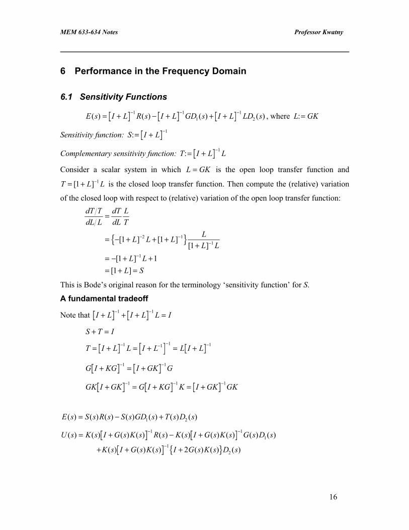
6 Performance in the Frequency Domain

6.1 Sensitivity Functions

E s I L R s I L GD s I L LD s( ) ( ) ( ) ( )= + − + + +− − −1 11

12 , where L GK:=

Sensitivity function: S I L:= + −1

Complementary sensitivity function: T I L:= + −1 L

L

Consider a scalar system in which is the open loop transfer function and

is the closed loop transfer function. Then compute the (relative) variation

of the closed loop with respect to (relative) variation of the open loop transfer function:

L GK=

T L= + −[ ]1 1

dT TdL L

dTdL

LT

L L L LL L

L LL S

=

= − + + ++

= − + += + =

− −−

−

[ ] [ ][ ]

[ ][ ]

1 11

1 11

2 11

1

m r

This is Bode’s original reason for the terminology ‘sensitivity function’ for S.

A fundamental tradeoff

Note that I L I L L I+ + + =− −1 1

S T I+ =

T I L L I L L I L= + = + = +− − − −1 1 1 1

G I KG I GK G+ = +− −1 1

GK I GK G I KG K I GK GK+ = + = +− − −1 1 1

E s S s R s S s GD s T s D s( ) ( ) ( ) ( ) ( ) ( ) ( )= − +1 2

U s K s I G s K s R s K s I G s K s G s D s

K s I G s K s I G s K s D s

( ) ( ) ( ) ( ) ( ) ( ) ( ) ( ) ( ) ( )

( ) ( ) ( ) ( ) ( ) ( )

= + − +

+ + +

− −

−

1 11

122l q

16


6.2 Sensitivity Peaks

)(max ωω

jSM S = , )(max ωω

jTT =M

Sensitivity peaks are related to gain and phase margin.

Sensitivity peaks are related to overshoot and damping ratio.

-1a

L j( )ω

L plane−

S a= 1

S L− = +1 1

S > 1 S < 1

Re

Im

6.3 Bandwidth

Bandwidth (sensitivity) ),0[21)(:max vjSvvBS ∈∀<= ωωω

Bandwidth (complementary sensitivity) ),(21)(:min ∞∈∀<= vjSvvBT ωωω

Crossover frequency ),0[1)(:max vjLvvc ∈∀≥= ωωω

Bandwidth is related to rise time and settling time.

6.4 Limits on Performance

17


7 Nominal Controller Design: Frequency Domain Perspective

7.1 Full State Feedback Controllers

The Quadratic Regulator Problem

( , ) ( ) ( ) ( ) ( ) ( ) ( )TT T T

f tJ x t x T Q x T x Qx u Ru dτ τ τ τ τ = + + ∫

Principle of Optimality & HJB Equation

Stability of Sol’ns to LQR

Consider the linear system x Ax= . Suppose V x with . Compute the time

rate of change of V along trajectories

( ) Tx Px= 0P >

T T TVV x x PAx x A Pxx

∂= = +∂

(1.1)

Suppose V x , . Then, clearly, the system is asymptotically stable,

as . Actually, if , we require only . Hence, if there exists a

that satisfies the Liapunov equation

TQ= − x 0Q >

det A

( ) 0x t →

0P >t → ∞ 0≠ 0Q ≥

(1.2) TPA A P Q+ = −

for any , the system is asymptotically stable provided det . As a matter of fact

this requirement is necessary, as well as sufficient, for asymptotic stability.

0Q ≥ 0A ≠

Now, consider the linear control system

x Ax Bu= + (1.3)

Suppose that so that the closed loop system is u Kx=

( )x A BK x= + (1.4)

Moreover, choose where 1 TK R B P−= − x

T

(1.5) 1T TPA A P PBR B P Q−+ − = −

Now, (1.5) can be rewritten

1( ) ( )TP A BK A BK P Q PBR B P−+ + + = − −

18


A Generalization of the Standard LQR

Consider, the more general performance index:

( , ) ( ) ( ) ( ) ( ) 2 ( ) ( ) ( ) ( )TT T T T

f tJ x t x T Q x T x Qx x Su t u Ru dτ τ τ τ τ = + + + ∫ τ

≥

)1

with , and Q S . We can reduce this problem to the standard case by

noting the identity (complete the square)

0R > 1 0R S−−

( ) ( ) (1 12T TT T T T Tx Qx x Su u Ru u R Sx R u R Sx x Q SR S x− − −+ + = + + + −

Define a new control

1 Tu u R S x−= +

so that the system equations become

( )1 Tx Ax Bu x A BR S x Bu−= + ⇒ = − +

τ τ

x

)1 T−

and in terms of the new control, the performance index is

( )1( , ) ( ) ( ) ( ) ( ) ( ) ( )TT T T T

f tJ x t x T Q x T x Q SR S x u Ru dτ τ τ− = + − + ∫

Thus, the problem has been recast in the from of the standard regulator problem. The

solution is

( )1 Tu R B P S−= − +

( ) ( ) (1 1 1TT T TP A BR S A BR S P PBR B P Q SR S− − −− + − − + −

Min-Max Control Consider a system by disturbances w t with performance outputs ( ) ( )y t

x Ax Bu Ewy Cx

= + +=

(1.6)

The disturbance is norm bounded, but otherwise unknown. Our goal is to find a state

feedback control that produces minimum quadratic cost for the ‘worst-case’ disturbance.

To make this statement precise, we set up the performance index:

(1.7) 2

0( , ) ( ) ( ) ( ) ( ) ( ) ( )T T TJ u w y t y t u t u t w t w t dtρ γ

∞ = + − ∫

19


where the weighting constants . By explicitly including the disturbances in the

cost in a negative way, stationary points of will be saddle points. We seek u t

that minimizes J while a perverse nature seeks that maximizes it. The optimization

problem is to find

, 0ρ γ >

( , )J u w

( )w t

( )

min max ( , )u w

J u w

Proposition: Consider the system (1.6) with performance index (1.7). Suppose that

1. has bounded energy, ( )w t

2. ( , )A B and ( , )A E are stabilizable,

3. ( , )A C is detectable.

Then, if the optimal solution exists, it is a unique saddle point of where ( , )J u w

1. The optimal min-max control is

, with ( ) ( )u t Kx t= 1 TK Bρ

= − S

2. The worst case disturbance is

2

1( ) ( )Tw t E Sx tγ

=

S is the unique, symmetric, nonnegative solution of the algebraic Riccati equation

2

1 1T T TA S SA S BB EE C Cρ γ

+ − − = −

T

Recall that solution of the Riccati equation can be carried out by eigen-decomposition of

its associated Hamiltonian matrix. As long as the Hamiltonian matrix has no eigenvalues

on the imaginary axis, the required decomposition can be performed. The Hamiltonian

matrix for the min-max optimization problem is

2

1 1T T

T T

A EE BBH

C C Aγ ρ

− = − −

20


Given the detectability/stabilizabilty assumptions it is possible to prove there exists a

minγ so that there are no eigenvalues of H on th imaginary axis provided minγ γ> . In fact,

when γ → ∞ we approach the standard LQR solution. For minγ γ=

n

, the controller is the

full state feedback controller. All other values of H∞ miγ γ≤ < ∞ produce valid min-

max controllers.

The condition that Re ( ) 0Hλ ≠ is equivalent to stability of the matrix

2

1 1T TA EE Bγ ρ

+ − B

Notice that the closed loop system matrix is

1 TA BBρ

−

Since 2/TEE γ is destabilizing, the feedback system has some margin of stability.

Solving the Riccati Equation Constructing the Solution

Computing Tools CARE Solve continuous-time algebraic Riccati equations.

[X,L,G,RR] = CARE(A,B,Q,R,S,E) computes the unique symmetric

stabilizing solution X of the continuous-time algebraic Riccati

equation

-1

A'XE + E'XA - (E'XB + S)R (B'XE + S') + Q = 0

or, equivalently,

-1 -1 -1

F'XE + E'XF - E'XBR B'XE + Q - SR S' = 0 with F:=A-BR S'.

When omitted, R,S and E are set to the default values R=I, S=0,

and E=I. Additional optional outputs include the gain matrix

-1

G = R (B'XE + S') ,

the vector L of closed-loop eigenvalues (i.e., EIG(A-B*G,E)),

21


and the Frobenius norm RR of the relative residual matrix.

[X,L,G,REPORT] = CARE(A,B,Q,...,'report') turns off error

messages and returns a success/failure diagnosis REPORT instead.

The value of REPORT is

* -1 if Hamiltonian matrix has eigenvalues too close to jw axis

* -2 if X=X2/X1 with X1 singular

* the relative residual RR when CARE succeeds.

[X1,X2,L,REPORT] = CARE(A,B,Q,...,'implicit') also turns off

error messages, but now returns matrices X1,X2 such that X=X2/X1.

REPORT=0 indicates success.

7.2 Output Feedback Controllers

The Classical H2 Problem – LQG The classical output feedback optimal control problem for SISO systems was solved

during the 2nd World War using a frequency domain formulation. It is referred to as the

Wiener-Hopf-Kolmogorov problem. Attempts to extend this result to the MIMO case

using frequency domain techniques were not fruitful. The MIMO problem was

formulated and solved in the state space by Kalman and coworkers around 1960. We

summarize the result here.

The Linear Quadratic Guassian (LQG) Problem - Setup

The standard problem formulation is as follows. The plant is described by

x Ax Bu wy Cx v

= + += +

The disturbances are independent, zero-mean white noise processes have

covariances,

,w v

( ) ( ) ( )

( ) ( ) ( )

T

T

E w t w W t

E v t v V t

τ δ

τ δ τ

= −

= −

τ

and

( ) ( ) 0TE w t v τ =

22


We seek that minimizes the performance index: ( )u t

0

1limT T T

TJ E x Qx u Ru dt

T→∞

= + ∫ 0, 0T TR R= ≥ = >, Q Q

Solution Summary

1ˆ( ), Tu Kx t K R B P−= = −

, 1T TPA A P PBR B P Q−+ − = − 0P ≥

( ) 1ˆ ˆ ˆ , Tx Ax Bu L y Cx L SC V −= + + − =

, 1T TSA AS SC V CS W−+ − = − 0S ≥

The Modern Paradigm We view the control design problem in terms of the diagram shown in Figure 1.

P

K

zw

u y

Figure 1. The so-called ‘modern paradigm’ views the plant in terms of two input sets:

disturbance and control inputs, and two out put sets: performance and measured

variables.

In the frequency domain the plant is characterized in terms of a transfer matrix:

zv

P PP P

wu

LNMOQP =LNM

OQPLNMOQP

11 12

21 22

Closing the loop with

u Kv=

Produces the closed loop transfer function

z Fw= , F P P I P K P= + − −11 12 22

121b g

23


In the state space the plant is defined as follows in terms of differential equations

1 2

1 11 12

2 21 22

x Ax B w B uz C x D w D uy C x D w D u

= + += + += + +

and, for convenience, we define the data structure

1 2

1 11 12

2 21 22

:

A B B

P C D DC D D

=

In the following we will make the following standing assumptions about the plant:

1. 11 0D =

2. 2( , )A B is stabilizable

3. is detectable 2( , )A C

4. with V 11 21

21

: xx xyT TT

xy yy

V VBV B D

V VD

= =

0≥ 0yy >

5. with [ ]11 12

12

: 0T

xx xuTTxu uu

R RCR C D

R RD

= =

≥ 0uuR >

Our goal is to find an output ( ) feedback controller that optimizes a performance

measure defined in terms of the performance variables (

y

z ) for some specified class of

disturbance inputs ( ). w

24


u ( ) 1sI A −− CB y

1W

2W

3W

4W

1w

2w

1z

2z

PLANT

E

x

Figure 2. The standard LQG problem recast in the modern paradigm.

Frequency Domain Formulation of the H2 Problem

The ‘energy norm’ or ‘2-norm’ of any scalar function ( )f t is defined by

2 222

1( ) : ( ) ( )2

f t f t dt F jω ωπ

∞ ∞

−∞ −∞= =∫ ∫ d

The latter obtained from Parseval’s theorem. This is easily generalized to vector a

function

2

2

1( ) ( ) ( ) ( ) ( )2

T Tf t f t F T dt F j F jω ωπ

∞ ∞

−∞ −∞= =∫ ∫ dω

Now, let us consider the control system shown in the figure. Suppose, we consider the

class of disturbances to be a zero mean white noise with

( ) ( ) ( )TE w t w t Iτ δ+ = τ

We seek to choose K so that the expected value of 2

( )z t is a minimum. Thus, we seek to

2

2min ( )

KE z t

Recall, . Now, compute [ ( )] 1tδ =L

25


1( ) ( ) ( ) ( )2

1tr ( ) ( )2

T T

T

z t z t dt Z j Z j d

Z j Z j d

ω ω ωπ

ω ωπ

∞ ∞

−∞ −∞

∞

−∞

= −

ω = −

∫ ∫

∫

2

2

2

2

1tr ( ) ( )21tr ( ) ( )

2

T

T

E z E Z j Z j d

F j F j d

F

ω ωπ

ω ω ωπ

∞

−∞

∞

−∞

ω = − = −

=

∫

∫

The H∞ Problem

We consider the same control design problem as above, except with the class of

disturbances defined by

2

( ) 1w t =

We seek to choose K such that the maximum of 2

( )z t over all disturbance inputs is

a minimum. Thus, we seek to

( )w t

2

21min max ( )

K wz t

=

Now, compute

1( ) ( ) ( ) ( )21 ( ) ( ) ( ) ( )

2

T T

T T

z t z t dt Z j Z j d

W j F j F j W j d

ω ω ωπ

ω ω ω ωπ

∞ ∞

−∞ −∞

∞

−∞

= −

= − −

∫ ∫

∫ ω

Now, we seek the maximum performance energy over all disturbances with unit norm. It

occurs when W j is aligned with the maximum eigenvalue of , ( )ω *F F

( )

( )2

2

1

22

1max ( ) ( ) ( ) ( ) ( )2max ( )

T T

wz t z t dt W j F j W j d

F j Fω

ω σ ω ω ωπ

σ ω

∞ ∞

−∞ −∞=

∞

=

= =

∫ ∫

Solution Summary

26


Proposition (H2 Output Feedback): Suppose is a unit intensity white noise signal, ( )w t

( ) ( ) ( )TE w t w I tτ δ= −τ . Then the unique, stabilizing, optimal controller that minimizes

2( )zwT s is

2 22

2 0

A LK

F

−=

were

( )( )

2 2 2 2 2 2 22

12 2 2

12 2 2

T Tuu xu

Txy yy

A A B F L C L D F

F R R B X

L Y C V V

−

−

= + + +

= − +

= − +

2

22 ,X Y satisfy the two Riccati equations

1 1

2 2 2 2 2 21 1

2 2 2 2 2 2

T Tr r uu xx xu uu xu

T Te e yy xx xy yy xy

T

T

X A A X X B R B X R R R R

A Y Y A Y C V C Y V V V V

− −

− −

+ − = − +

+ − = − +

( )( )

12

12

Tr uu

e xy yy

A A B R R

A A V V C

−

−

= −

= −

xu

( ) 1sI A −− 2F2L

2B

2C

22D

y ux-

27


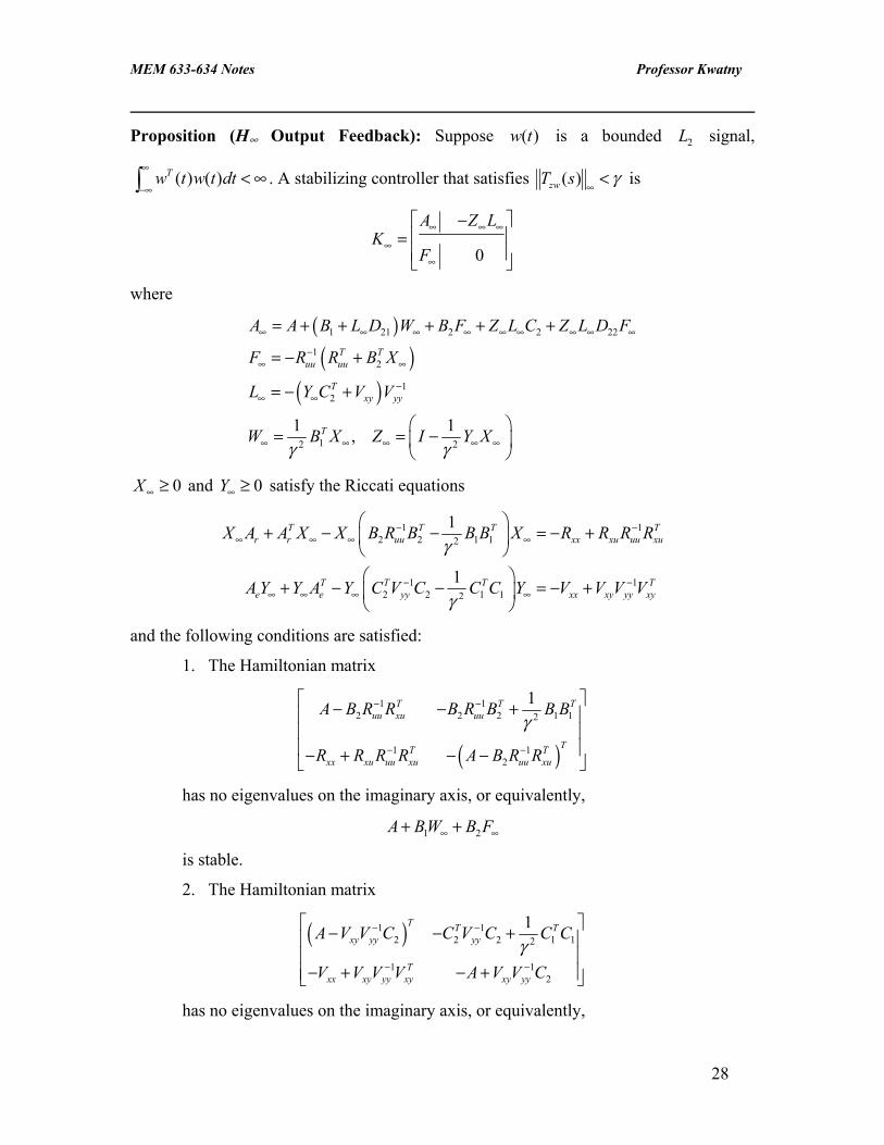
Proposition (H∞ Output Feedback): Suppose is a bounded signal,

. A stabilizing controller that satisfies

( )w t 2L

( ) ( )Tw t w t dt∞

−∞< ∞∫ ( )zwT s γ

∞< is

0

A Z LK

F

∞ ∞

∞∞

∞ − =

where

( )( )

( )

1 21 2 2 22

12

12

12 2

1 1,

T Tuu uu

Txy yy

T

A A B L D W B F Z L C Z L D F

F R R B X

L Y C V V

W B X Z I Y Xγ γ

∞ ∞ ∞ ∞ ∞ ∞ ∞ ∞ ∞

−∞ ∞

−∞ ∞

∞ ∞ ∞ ∞ ∞

= + + + + +

= − +

= − +

= = −

0X ∞ ≥ and Y satisfy the Riccati equations 0∞ ≥

1 12 2 1 12

1 12 2 1 12

1

1

T T Tr r uu xx xu uu xu

T T Te e yy xx xy yy xy

T

T

X A A X X B R B B B X R R R R

A Y Y A Y C V C C C Y V V V V

γ

γ

− −∞ ∞ ∞ ∞

− −∞ ∞ ∞ ∞

+ − − = − +

+ − − = − +

and the following conditions are satisfied:

1. The Hamiltonian matrix

( )

1 12 2 2 2

1 12

1T Tuu xu uu

TT Txx xu uu xu uu xu

A B R R B R B B B

R R R R A B R R

γ− −

− −

− − + − + − −

1 1T

has no eigenvalues on the imaginary axis, or equivalently,

1 2A BW B F∞ ∞+ +

is stable.

2. The Hamiltonian matrix

( )1 1

2 2 2 12

1 12

1T T Txy yy yy

Txx xy yy xy xy yy

A V V C C V C C C

V V V V A V V Cγ

− −

− −

− − + − + − +

1

has no eigenvalues on the imaginary axis, or equivalently,

28


2 12

1 TA L C Y C Cγ∞ ∞+ + 1

γ

is stable.

3. , where 2( )Y Xρ ∞ ∞ < ( ) ( )max i iρ ⋅ = ⋅λ is the spectral radius.

( ) 1sI A −− F∞Z L∞ ∞

2B

2C

22D

y ux

1 21B L D∞+ W∞

w

-

29


8 Robust Stability & Nyquist Analysis

8.1 SISO Nyquist Analysis

30


Guaranteed Gain and Phase Margin

Proposition: Suppose is the maximum sensitivity peak. Then SM

α±≥

11GM ,

±≥

2sin2 αPM , SM1=α

Proof: The proof is easily obtained from the geometry shown in the figure

GH-plane

-1

1 1R Sa

−= =

1 12sin2a

θ − =

1 1 a−

1 1 a+

8.2 MIMO Nyquist Analysis

Recall that the closed loop poles are roots of the polynomial

[ ]( ) ( )det ( )Ld s d s I L s= +

If the open loop system is stable, then to assess stability of the closed loop system we

need only be concerned with the zeros of

( ) det ( )F s I L= + s

Nyquist analysis still applies with det ( )I L s+ replacing 1 . Specifically we have: ( )L s+

Z P N= −

where:

Z=number of closed loop poles in the RHP

P=number of open loop poles in the RHP

N=number of counterclockwise encirclements of the F-plane origin by . ( )F C

31


Suppose that the closed loop system is asymptotically stable. Then the Nyquist

det ( ) 0, , 0I L s s jσ ω σ+ ≠ ∀ = + ≥

8.3 M ∆ - Structure

Models of Uncertainty

G G EG G I EG I E G

G G I EG

G G I E

G I E G

p

p

p

p

p

p

= += += +

= −

= −

= −

−

−

−

( )( )

( )

( )

( )

1

1

1

, , E W W= 1∆ 2 ∆ ∞ < 1

M W M W= 1 0 2 ,

M K I GK KSM K I GK G TM GK I GK TM I GK G SGM I GK SM I GK S

I

I

01

01

01

01

01

01

= + =

= + =

= + =

= + =

= + =

= + =

−

−

−

−

−

−

( )( )

( )( )( )( )

8.4 Small Gain Theorem

Consider a feedback loop with open loop transfer matrix . Then we define the

spectral radius:

L s( )

ρ ω λ ωL j L ji i( ) max ( )b g b g=

Theorem (Spectral radius stability theorem). Consider a system with stable open loop

transfer function . Then the closed loop is stable if L s( )

ρ ω ωL j( ) ,b g < ∀1

Theorem (Small gain theorem). Consider a system with stable open loop transfer

function . Then the closed loop is stable if L s( )

L j( ) ,ω ω< ∀1

where L denotes any norm satisfying AB A B≤ ⋅ .

32


8.5 Robust Stability of the M ∆ - Structure

Theorem (Robust stability for unstructured perturbations). Assume that the nominal

system M s( ) is stable and that the perturbations are stable. Then the -system is

stable for all perturbations satisfying

∆( )s M ∆

∆ ∞ ≤ 1 if and only if

σ ω ωM j( ) ,b g < ∀1 ⇔ M ∞ < 1

Notice that:

RS ⇔ M ∞ < 1 ⇔ W M W1 0 2 1∞

<

Special case

G G I wp = + <∞( ),∆ ∆ 1 ⇔ wT ∞ < 1

33


9 Robust Performance

34


10 Some Complex Variable Concepts

For proper, stable, minimum phase systems: gain ⇔ phase:

H( )0 0>

10.1 Analytic Functions

A function of a complex variable s is analytic at if it is differentiable on a

neighborhood of .

)(sf Cs ∈0

0s

Example:

)()(

)()()()(

)(1

1

sdsn

pspsqsqs

KsHn

m =−−−−

=

is analytic everywhere except at its poles. Notice that , so )(ln)(lnln sdsnH −=

ds

sddsdds

sndsnds

Hd )()(

1)()(

1ln −=

hence ln H is analytic everywhere except at poles and zeros of H.

Cauchy Integral Theorem:

Suppose that f is analytic on a domain D, and suppose ∂Ω is any piecewise smooth

simple closed curve in D, then

∫ Ω∂= 0)( dssf

Cauchy Integral Formula:

Suppose that ∂Ω is a simple closed curve ∂Ω in the complex plane, and f is an analytic

function on ∂Ω and its interior Ω. Then

∫ Ω∂ −= dz

szzf

jsf )(

21)(π

, for all s . ∈Ω

Residue Theorem Suppose ( )f s is an analytic function having isolated singular points. Let C be a simple

closed curve that encloses n singular points having residues . Then , 1, ,ic i n= …

1

( ) 2n

kiC

f s ds j cπ=

= ∑∫

35


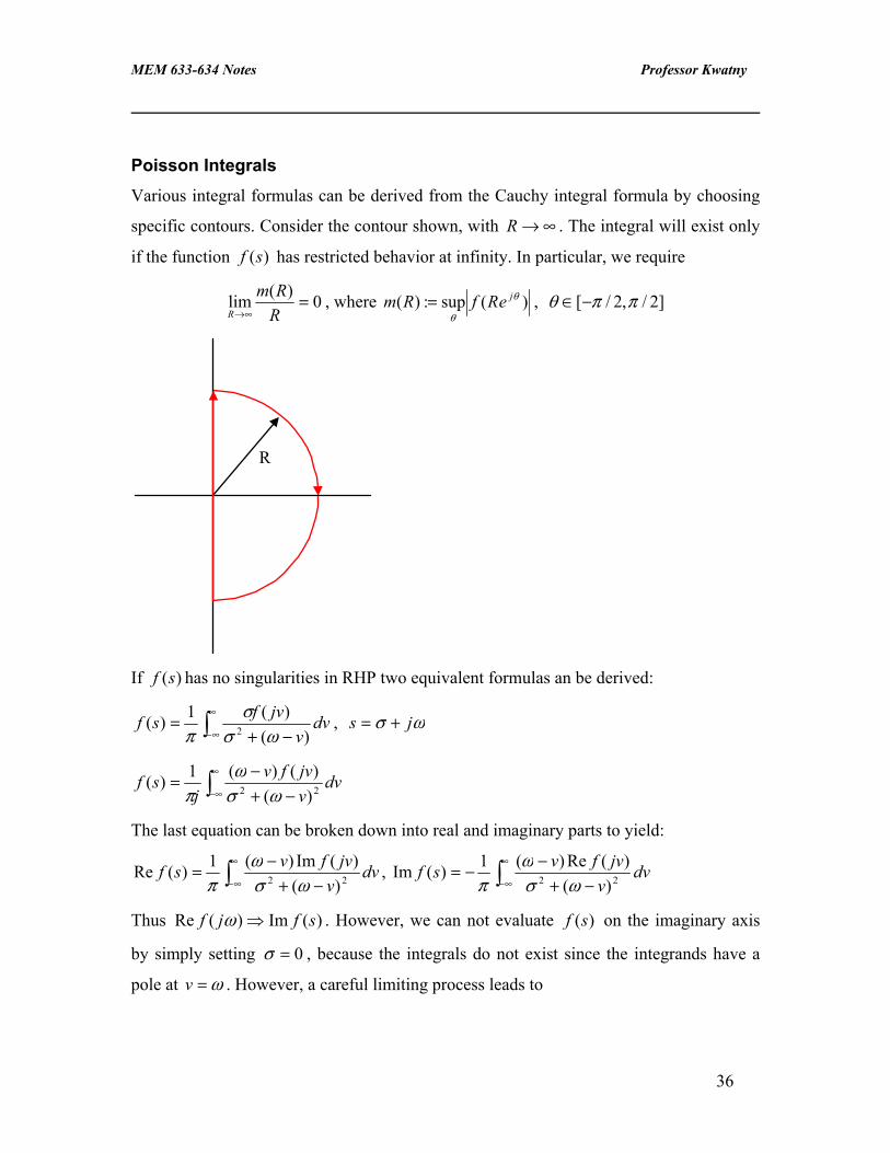
Poisson Integrals Various integral formulas can be derived from the Cauchy integral formula by choosing

specific contours. Consider the contour shown, with . The integral will exist only

if the function has restricted behavior at infinity. In particular, we require

∞→R

)(sf

0)(lim =∞→ R

RmR

, where )(sup:)( θ

θ

jeRfRm = , ]2/,2/[ ππθ −∈

R

If has no singularities in RHP two equivalent formulas an be derived: )(sf

∫∞

∞− −+= dv

vjvfsf

)()(1)( 2 ωσ

σπ

, ωσ j+=s

∫∞

∞− −+−= dv

vjvfv

jsf 22 )(

)()(1)(ωσ

ωπ

The last equation can be broken down into real and imaginary parts to yield:

∫∞

∞− −+−= dv

vjvfvsf 22 )(

)(Im)(1)(Reωσ

ωπ

, ∫∞

∞− −+−−= dv

vjvfvsf 22 )(

)(Re)(1)(ωσ

Im ωπ

Thus )(Im)(Re sfjf ⇒ω . However, we can not evaluate on the imaginary axis

by simply setting

)(sf

0=σ , because the integrals do not exist since the integrands have a

pole at ω=v . However, a careful limiting process leads to

36


ααα

ωπ

ωα

dd

ejfdjf ∫∞

∞−=

2cothlog)(Re1)(Im

Suppose is a transfer function. Then consider )(sH

)(log)( sHsf =

for which )()(Re sHsf = and . Then )()(Im sHsf ∠=

ααα

ωπ

ωα

dd

ejHdjH ∫

∞

∞−=∠

2cothlog

)(log1)(

Since must be analytic in RHP, can have neither poles nor zeros in RHP. )(sf )(sH

Bode Waterbed Formula Application of the Cauchy Integral Formula to systems with relative degree 2 or greater:

(Waterbed effect)

ln ( )S j d piORHP poles

ω ω π0

∞z ∑=

ln ( )T j dqiORHP zeros

ω ωω

π0 2

1∞z ∑=

Example: Stable plant

L ss

( )( )

=+11 2

È

2 4 6 8w

-0.6

-0.4

-0.2

SÈ Bode Integral Formula

37


10.2 Parseval’s Theorem

A simple, but important formula is given by Parseval’s theorem. Suppose the functions

f t f t1 2( ), ( ) have Laplace transforms , respectively. Then we can write F s F s1 2( ), ( )

f t f t dt L F s f t dt

jF s e ds f t dt

jf t e dt F s ds

jF s F s ds

st

j

j

st

j

j

j

j

1 21

1 2

1 2

2 1

2 1

121

21

2

( ) ( ) ( ) ( )

( ) ( )

( ) ( )

( ) ( )

−∞

∞ −

−∞

∞

− ∞

∞

−∞

∞

−∞

∞

− ∞

∞

− ∞

∞

z zzzzzz

=

=

=

= −

π

π

π

f t dtj

F s F s ds

F j F j d

F j d

j

j2

2

121

21

2

( ) ( ) ( )

( ) ( )

( )

−∞

∞

− ∞

∞

−∞

∞

−∞

∞

z zzz

= −

= −

=

π

πω ω ω

πω ω

38


39


11 Normed Linear Spaces

11.1 Norms and Normed Linear Spaces

Definition: A linear space over the field R (or C) is a set of elements x, y, … such

that

For each pair x y, ∈ , the sum is defined x y+ ∈ and x y y x+ = +

there is an element 0 such that for every ∈ x ∈ , x x+ =0

for any numbers a b (or C) scalar multiplication is defined, R, ∈ ax ∈ , and 1⋅ =x x ,

, and ( for all ( ) ( )ab x a bx b= = ( )ax )a b x ax bx+ = + x y, ∈ .

A linear space is a normed linear space if to each element x ∈ there corresponds a real

number x called the norm of x which satisfies:

x for x> ≠0 0 0, = 0

x y x y+ ≤ + (triangle inequality)

ax a x= ⋅ for all a R∈ (or C) and x ∈

Examples of normed linear spaces:

1. The spaces R and C with x x= , the absolute value of x.

2. The real and complex Euclidean spaces Rn and Cn the spaces of scalar real or

complex n-tuples with norm: x xii

n

= FHGIKJ

2/

=∑

1

1 2

3. The spaces l , space np ( ) Rn or Cn with norm: x xip

i

n p

= FHGIKJ=

∑1

1/

4. The space l , space n∞ ( ) Rn or Cn with norm: x x n= max , ,1 …m x r . The notation

is adopted because

max , , lim/

x x xn p ip

i

n p

11

1

…m r = FHG

IKJ→∞

=∑

Prove this for the case . n = 2

40


5. The function spaces consisting of (complex-valued) integrable

functions with bounded norm:

L a b pp[ , ], 1≤ ≤ ∞

a b, ]f t t( ), [∈ f f t dpp

a

b p

= tLNM

OQPz ( )

/1

, 1≤ < ∞p

and f ft a b∈

= sup ([ , ]

t)∞ .

6. The set of complex valued m matrices, denoted n× Cm n× , with norm

1/ 2

2 *

, 1trace( ) ( )

n

ij ii j i

A a A A σ=

= = = ∑ ∑ A , or the norm A A= σ b g

This is sometimes called the Frobenius norm.

7. Time-Domain (Signal) spaces. Consider complex vector valued time functions

defined on the interval (or, ). The appropriate p-

norm is

f t Rn( ) ∈ t ∈ −∞ ∞[ , ] t ∈ ∞[ , ]0

f f tp ip

i

n p

= dtFHG

IKJ=

−∞

∞

∑z ( )/

1

1

, 1≤ < ∞p and f ft i i∞ = sup max ( )e jt .

For p = 2 we can use Parseval’s theorem to obtain

f f t dt F j d F F dii

n

ii

n

2

2

1

1 22

1

1 2 1 2

= FHGIKJ = FHG

IKJ = FH IK

=−∞

∞

=−∞

∞

−∞

∞

∑z ∑z z( ) ( )/ /

*/

ω ω ω

8. Frequency-Domain Spaces. Consider the functions , F j Cn( )ω ∈ −∞ < < ∞ω

F F jpp

i

n p

= dFHG

IKJ=

−∞

∞

∑z12 1

1

πω ω( )

/

, 1≤ < ∞p and F F j F∞ = sup ( ) ( )*

ωω ωe jj .

The space of all frequency functions with bounded p-norm is often designated

. Lp

9. The space of functions that are analytic in the open right half

plane, R with

F s F C Cn( ), : →

e( )s > 0

F F jp

p

i

n p

= + dFHG

IKJ> =

−∞

∞

∑zsup ( )/

ξ πξ ω ω

0 1

11

2, 1≤ < ∞p and

F F s F ss

∞>

= sup ( ) ( )*

0e j

The space of functions with bound p-norm is the Hardy space . Hp

41


For almost all ω, lim ( ) ( )ξ

ξ ω ω→

+ = ∈0

F j F j pL

x

. Moreover, the supremum occurs

on the imaginary axis.

11.2 System Norms/ Induced Norms

Consider a mapping A from one normed linear space to another . That is,

y A=

One way to view the ‘magnitude’ of the action A is consider its ‘gain,’ that is the ratio:

y x/ . The ratio will depend on the specific choice of input x. So, we choose the one

that produces the largest ratio, i.e.:

Ayx

Axxx x

= =≠ ≠

max max0 0

Because A is linear, it is clear that the gain is independent of the size of x so we could

rescale and equivalently define

A Ax

==

max1

x

Now, the definition depends on the specific choices of input and output spaces and .

Suppose that the p-norm is appropriate for both spaces, then we can define

AAx

xxαββ

α

=≠

max0

These induced norms have the product property:

A B A B≤

Transfer matrix norms Consider systems described by l m× stable, proper transfer matrices: Y s G s U s( ) ( ) ( )=

We will consider two transfer function norms:

H2 Norm

G s G j G j d G j dii

G

( ) tr ( ) ( ) ( )*/ rank[ ] /

2

1 2

1

1 21

21

2= FHG

IKJ =FHG

IKJ−∞

∞

=−∞

∞z ∑zπω ω ω

πσ ω ω

H∞ Norm

42


G s G j( ) sup ( )∞ =ω

σ ω

Suppose that the input space is equipped with the norm and the output space with the

. Then we have

L2

L∞

Y U G∞ = sup * *

ω GU

so that

G UU2 12

∞ == max sup * *

ω G GU

Suppose that the input and output spaces are equipped with the norm. Then we have L2

Y U G G22 = * * U

so that

G U j G j G j U j dU

j

22 1=

= −∞

∞zmax ( ) ( ) ( ) ( )* *ω ω ω ω ω

We need to choose U to maximize the result. Clearly, at each ω we maximize the kernel

by aligning U with the largest eigenvector of G G* so that we have

U G GU j U j* * ( ) ( ) ( )ω σ ω ω= 2 where σ ωG j( )b g is the maximum singular value of G.

Then we need to concentrate all of the energy in U at the frequency at which σ is a

maximum

G G∞ = sup ( )ω

jσ ωb g Computing the H2 Norm

AL L A BBc cT T+ + = 0 , A L L A C CT

o oT+ + = 0

G CL C B L BcT T

o2

1 2 1 2= =tr( ) tr( )

/ /

Computing the H∞ Norm

Find smallest γ > 0 such that H has no eigenvalues on the imaginary axis.

HA BB

C C A

T

T T=

− −

L

NMM

O

QPP

12γ

43


1

Notes on Linear Robust Control - Drexel...

Documents

Transcript of Notes on Linear Robust Control - Drexel...