Notes of ODE Recitations - NYU Courant · Notes of ODE Recitations Jiajun Tong October 29, 2016 1...

Notes of ODE Recitations

Jiajun Tong

October 29, 2016

1 The Recitation on September 16, 2016

Key points: Second order ODE with constant coefficients, harmonic oscillator.

Reference: W.E. Boyce and R.C. DiPrima [2], § 3.7-3.8.

1.1 Modeling a harmonic oscillator (a spring-mass system)

Let u(t) be the vertical displacement of the mass from its equilibrium position. Then its accel-

eration would be u′′(t). The equation of u(t) writes as

mu′′(t) = −ku(t)− γu′(t) + F (t).

Here,

• m > 0 is the mass.

• k > 0 is the spring constant and the spring force −ku(t) is modeled to be proportional to u(t)

(i.e. Hooke’s law). The minus sign shows that it is always a restoring force which pulls the

mass back towards the equilibrium.

• γ ≥ 0 is the damping constant. The damping force may come from the medium (e.g. air,

water, or honey), the spring or other sources. It has a minus sign since it prevents the mass

from moving.

• F (t) is the external force, assumed to be independent of u.

• Initial data could be provided as well, e.g. u(0) = u0 and u′(0) = v0.

1.2 Undamped free vibrations

We assume γ = 0 and F (t) ≡ 0 in this case. The equation becomes

mu′′ + ku = 0. (1)

To solve such homogeneous linear ODE with constant coefficients,

1. We write down the characteristic polynomial mr2 + k = 0, where r ∈ C. The concept of

characteristic polynomial comes from plugging the ansatz u(t) = ert into the equation (1). It

is explained in [1] in § 2.2.

1

2. Find the roots of the characteristic polynomial. r± = ±i√k/m. This implies that er+t and

er−t are both solutions for (1).

3. By linearity, u(t) = C1er+t + C2er−t = C1eit√k/m + C2e−it

√k/m is a general solution of

(1), with C1 and C2 being arbitrary complex constants. Conversely, any general solution of

(1) could be written into this form, which is explained in [1] in § 2.3. C1 and C2 could be

determined by the initial data.

4. You may wish to rewrite the general solution as u(t) = C̃1 cos(t√k/m) + C̃2 sin(t

√k/m) to

avoid complex numbers.

1.3 Damped free vibration

Here we only assume F (t) ≡ 0. Following the same recipe as above, we find

1. The characteristic polynomial mr2 + γr + k = 0. It has two roots

r± =−γ ±

√γ2 − 4mk

2m.

2. Discussions based on the sign of γ2 − 4mk.

Case 1.1 (γ2 − 4mk > 0, overdamped case). Since 0 < γ2 − 4mk < γ2, we get two distinct

negative roots. The general solution writes as u(t) = C1er+t +C2er−t. It exponentially decays

as t → +∞. We remark that γ2 − 4mk > 0 happens if the friction is large. Hence, you can

not see oscillation in this case — the mass just gets closer and closer to the equilibrium.

Case 1.2 (γ2−4mk = 0, critically damped case). We get r± = −γ/2m, a root with multiplicity

2! The general solution will have a different form when there are repeated roots. See [1] in § 2.2

for a clever derivation instead of merely a verification done in the recitation. In our case, that

gives general solution

u(t) = C1e−γt/(2m) + C2te−γt/(2m), (2)

where C1 and C2 are given by the initial condition. It is also an exponentially-decaying solution

— no oscillation.

Case 1.3 (γ2 − 4mk < 0, underdamped case). We get two conjugate complex roots,

r± = − γ

2m± i√

4mk − γ22m

, − γ

2m± iω.

The general solution would be

u(t) = C1er+t + C2er−t = e−γt/(2m)(C1eiωt + C2e−iωt

)= e−γt/(2m)

(C̃1 cos(ωt) + C̃2 sin(ωt)

).

This corresponds to a system with small friction/damping. The solution is oscillatory, with its

amplitude exponentially decaying.

1.4 Undamped forced vibration

Here we assume γ = 0 and F (t) 6≡ 0. For simplicity we also take m = 1 and k = 1. The equation

becomes

u′′(t) + u(t) = F (t). (3)

2

To solve such non-homogeneous second order ODE with constant coefficients, we need to (see [1] in

§ 2.6)

1. Study the homogeneous one, i.e. with F (t) = 0, and find out a general solution. We have

already done that before, i.e.

uhom(t) = C̃1 cos t+ C̃2 sin t,

with C̃1 and C̃2 to be determined.

2. Find a particular solution up(t) for the non-homogeneous equation. (Explained below.)

3. The final solution would be u(t) = up(t) + uhom(t). The constants C̃1 and C̃2 should be

determined by the initial data.

To demonstrate the second step above, which is the most important one, we use two examples

F1(t) = cos(t/2) and F2(t) = cos t. We may follow the methods in [1] in § 2.6 or § 2.11 to find out

the solution, which is rather systematic. Here we shall use a good guess to find the solution instead.

First assume up(t) has the form of ert. Plugging it into the left hand side of (3), we find

(ert)′′ + ert = (r2 + 1)ert.

Note that r2+1 is exactly the characteristic polynomial corresponding to the homogeneous equation

u′′ + u = 0. r2 + 1 6= 0 if and only if r 6= ±i. Since F1(t) = 12 (eit/2 + e−it/2), we take r = ±i/2.

Using

(e±it/2)′′ + e±it/2 =3

4e±it/2,

we know that for F1(t),

up(t) =2

3(eit/2 + e−it/2) =

4

3cos(t/2).

Therefore, given F1(t), we will end up with an oscillatory solution with amplitude being bounded in

time.

For F2(t) = 12 (eit + e−it), taking r = ±i will not work any longer as (e±it)′′ + e±it = 0. Hence,

we test a new form of solution tert, which comes from the general solution of homogeneous equation

when there are repeated roots (see (2)). We find that

(tert)′′ + tert = r2tert + 2rert + tert = (r2 + 1)tert + 2rert.

Note that (r2 + 1) here is the characteristic polynomial. Now we take r = ±i and find

(te±it)′′ + te±it = ±2ie±it.

There is a non-trivial term left on the right hand side! Therefore, combining this with F2(t) =12 (eit + e−it), we find

up(t) =1

4iteit − 1

4ite−it =

1

2t sin t

is the particular solution corresponding to F2(t). The final solution is given by

u(t) =1

2t sin t+ C̃1 cos t+ C̃2 sin t,

where C̃1 and C̃2 are given by the initial data. We remark that the solution is still oscillatory;

however, its amplitude has a linear growth! This phenomenon is called resonance, which is very

important in math, physics and engineering. This results from the fact that the frequency of the

forcing F2(t) agrees with the intrinsic frequency of the spring-mass system (i.e. r = ±i).

3

1.5 Damped forced vibration

We did not cover this part in the recitation. Please read § 3.8 in [2] if you are interested.


Key points: Practice quiz 1, linear ODEs with constant or variable coefficients.

Problem 2.1. Find a basis of solutions on R of: (a) y′′ − y = 0; (b) y′′ + y = 0.

Solution. We simply write down the characteristic polynomials, find out their roots and then write

down the basis.

(a) The characteristic polynomial is s2 − 1 = 0. Its roots are s = ±1. A basis of solutions on R is

then given by {ex, e−x}.

(b) The characteristic polynomial is s2 + 1 = 0, Its roots are s = ±i. A basis of solutions on R is

then given by {eix, e−ix}, or equivalently {cosx, sinx}.

If I understand it correctly, here “a basis of solutions on R” means solutions defined on R instead

of real-valued solutions.

Problem 2.2. Find a basis of solutions on R of the homogeneous constant-coefficient linear ODE

whose characteristic polynomial is

p(s) = is(s+ i)2(s− i)3.

Solution. There is no need to recover the original ODE. The polynomial has roots 0, −i and i, with

multiplicity 1, 2 and 3 respectively. Hence, a basis of solutions on R is given by

{1, e−ix, xe−ix, eix, xeix, x2eix}.

Recall that a repeated root s∗ with multiplicity m > 1 corresponds to general solutions

{es∗x, xes∗x, · · · , xm−1es∗x}.

Problem 2.3 (True/False Questions).

(a) The function

(−π/2, π/2) 3 x 7→ (cosx) ln(cosx) + x sinx

is a solution of the ODE y′′ + y = secx.

(b) The ODE y′′ + xy′ + x2y = sin(x+ y) is linear.

(c) If φ1, φ2 : R→ C are linearly independent and differentiable, then their Wronskian,

W (φ1, φ2) = x 7→ det

(φ1(x) φ2(x)

φ′1(x) φ′2(x)

)

is never zero.

4

(d) If p, q, r : R→ C are continuous, the solutions on R of the ODE y′′′+p(x)y′′+q(x)y′+r(x)y = 0

form a 3-dimensional vector space.

Solution.

(a) True. To see whether a function is a solution, we need to check if it is admissible (we need y

and its derivatives to be well-defined), and if the equation is satisfied. Since x ∈ (−π/2, π/2),

cosx ∈ (0, 1]. Hence, y is well-defined. We calculate that

y′ = − sinx ln(cosx) + cosx · − sinx

cosx+ sinx+ x cosx = x cosx− sinx ln(cosx),

y′′ = cosx− x sinx− cosx ln(cosx)− sinx · − sinx

cosx=

1

cosx− x sinx− cosx ln(cosx),

both of which are well-defined. Hence,

y′′ + y = x cosx− sinx ln(cosx) +1

cosx− x sinx− cosx ln(cosx) = secx.

This shows the given function is a solution of the ODE y′′ + y = secx.

(b) False, because sin(x+y) is nonlinear in y. To determine whether an equation is linear, we simply

look at the unknown function y and its derivatives, instead of the independent variable x. As

more examples, y′′ + xy′ + x2y = 0 is linear while y′′ + xy′ + xy2 = 0 or y′′ + y′2 + xy = 0 are

nonlinear.

(c) False. Since φ1 and φ2 do not have to be solutions of a second order linear ODE, the statement

is false. A counterexample is that φ1 = x and φ2 = x2 at x = 0.

Remark 2.1. We recall that φ1 and φ2 are said to be linearly dependent, iff for ∃ (c1, c2) 6= (0, 0),

such that c1φ1 + c2φ2 ≡ 0 on R. See [1] in § 2.4.

Remark 2.2. We also recall that if φ1 and φ2 turn out to be two solutions of one linear second-

order ODE L(y) = 0 on a bounded interval I ⊂ R (that I is a bounded interval is a technical

assumption for simplicity), then the following three statements are equivalent:

(a) φ1 and φ2 are linearly independent in I.

(b) ∀x ∈ I, W (φ1, φ2)(x) 6= 0. See Theorem 6 in [1] § 2.4.

(c) ∃x0 ∈ I, such that W (φ1, φ2)(x0) 6= 0. See Theorem 7 in [1] § 2.4.

Therefore, the statement is true if φ1 and φ2 are two linearly independent solutions of L(y) = 0.

(d) True, by the existence (see Theorem 1 in [1] § 3.2) and uniqueness (see Theorem 3 in [1] § 3.2) of

the solutions. Equivalently, we can also apply Theorem 4 in [1] § 3.3. To be more precise, in our

case, we know that for ∀ (α1, α2, α3) ∈ C3, there exists a unique solution y of L(y) = 0 satisfying

that y(0) = α1, y′(0) = α2 and y′′(0) = α3. So the set of all the solutions is isomorphic to a

3-dimensional vector space on C.

Problem 2.4. Find a solution on I = (0,+∞) of the ODE

x2y′′ − 2y = 3x− 1 (4)

using variation of parameters, given the homogeneous solutions φ1(x) = x2 and φ2(x) = x−1.

5

Solution. We assume a particular solution for the non-homogeneous equation has the following form

yp(x) = u1(x)φ1(x) + u2(x)φ2(x).

By variation of parameters, it suffices to solve the following equation

u′1φ1 + u′2φ2 = 0,

u′1φ′1 + u′2φ

′2 =

3x− 1

x2. (See Remark 2.3 below.) (5)

Since φ′1(x) = 2x and φ2(x) = −x−2, this gives

x2u′1 + x−1u′2 = 0,

2xu′1 − x−2u′2 =3x− 1

x2.

The solution is

u′1 = x−2 − 1

3x−3, u′2 = −x+

1

3,

which gives

u1(x) = −x−1 +1

6x−2 + c1, u2(x) = −1

2x2 +

1

3x+ c2.

Therefore, the particular solution is

yp(x) = u1(x)φ1(x) + u2(x)φ2(x) = −3

2x+

1

2+ (c1φ1 + c2φ2).

The c1φ1 + c2φ2 could be omitted since eventually the solution is represented as

y(x) = yp(x) + C1φ1(x) + C2φ2(x) =

(−3

2x+

1

2

)+ C̃1φ1(x) + C̃2φ2(x),

where ci’s could be absorbed into C̃i’s.

Remark 2.3. In the recitation, I emphasized that one needs to be careful to find out the correct

right-hand side in (5). Although one can naively apply the recipe of variation of parameters, it is of

course better to understand the method first so that some mistakes could be avoided. For example,

the recipe in the textbook and the lectures only apply to ODEs whose coefficient of the highest

derivative is 1. In such case, one only needs to put the right-hand side of the equation in the place

of b(x) in the context of variation of parameters. However, it is not the case here, so one needs to

first normalize the equation by dividing x2 on both sides of the equation.

To understand why the coefficient of the highest derivative could play a role, let us recall how the

variation of parameters works. Starting from the form of the particular solution yp(x) = u1(x)φ1(x)+

u2(x)φ2(x), we take derivatives to find that

y′p = (u′1φ1 + u′2φ2) + u1φ′1 + u2φ

′2.

We assume the part in the round brackets to vanish so that the formula is simplified. In this way,

we obtain y′p as if u1 and u2 are constants — derivatives of ui’s do not show up! This is the main

idea of variation of parameters. Then we calculate the second derivative

y′′p = (u1φ′1 + u2φ

′2)′ = (u′1φ

′1 + u′2φ

′2) + u1φ

′′1 + u2φ

′′2 .

Hence, plugging yp and its derivatives into (4), we find that

x2y′′ − 2y = x2(u′1φ′1 + u′2φ

′2) + u1[x2φ′′1 − 2φ1] + u2[x2φ′′2 − 2φ2].

By assumption, the terms in the square brackets vanish! Hence, we need x2(u′1φ′1 + u′2φ

′2) = 3x− 1

so that (4) is satisfied.

6

Problem 2.5. Given the solution φ(x) = x−1 on I = (0,+∞) of the ODE

2x2y′′ + 3xy′ − y = 0, (6)

apply reduction of order to find a linearly independent solution on I.

Solution. We assume the other linearly independent solution to be y = uφ. Plugging it into (6), we

find that

2x2(uφ)′′ + 3x(uφ)′ − (uφ) = 2x2(u′′φ+ 2u′φ′ + uφ′′) + 3x(u′φ+ uφ′)− uφ

= 2x2φu′′ + (4x2φ′ + 3xφ)u′ + [2x2φ′′ + 3xφ′ − φ]u.

By assumption, the terms in the square bracket vanish. (This is the main idea of reduction of order,

i.e. by assuming y = uφ, the coefficient of zeroth-order term of u is L(φ) = 0.) By letting v = u′,

we find that

2x2φv′ + (4x2φ′ + 3xφ)v = 0.

Using the fact that φ = x−1 and φ′ = −x−2, we obtain 2xv′ − v = 0. The solution is given by

v(x) = Cx1/2.

See [1] in § 1.5 and § 1.7 for the method of solving first-order linear ODEs. Here C is an arbitrary

non-zero constant. We shall abuse this notation in the sequel, i.e. the value of C may change from

formula to formula. Hence, u′ = Cx1/2, and thus u = Cx3/2. The other solution of (6) is therefore

given by

y = uφ = Cx1/2.

Thanks to the linearity, we may take C = 1 here.


Key points: the annihilator method, Quiz 1.

Problem 3.1 ([1] § 2.11, Exercise 1(g)). Use the annihilator method to find a particular solution of

y′′ + iy′ + 2y = 2 cosh(2x) + e−2x. (7)

Solution. Denote L =(ddx

)2+ i ddx + 2. To apply the annihilator method, we rewrite the right-hand

side of (7) as sum of exponential functions

2 cosh(2x) + e−2x = e2x + 2e−2x.

Since (d

dx− 2

)e2x =

de2x

dx− 2e2x = 0,(

d

dx+ 2

)e−2x =

de−2x

dx+ 2e−2x = 0,

we construct a new differential operator

M ,

(d

dx− 2

)(d

dx+ 2

).

7

It is obvious that

Me2x =Me−2x = 0.

Applying M to both sides of (7), we find that

MLy =M(e2x + 2e−2x) = 0.

Note that we choosing M in this way, the right-hand side of the above equation vanishes and it

becomes a homogeneous one. This is why the method is call the annihilator method. Now we simply

solve the homogeneous equation MLy = 0 as usual. We write down its characteristic equation

(s− 2)(s+ 2)(s2 + is+ 2) = (s− 2)(s+ 2)(s+ 2i)(s− i).

Its roots are 2, −2, −2i and i. Hence, the general solution of MLy = 0 could be written as

y(x) = C1e2x + C2e−2x + C3e−2ix + C4eix. (8)

We note that the last two terms give a general solution of Ly = 0. Since any solution of (7) could

be written as sum of a particular solution yp(x) and linear combinations of general solutions of

Ly = 0, i.e. y(x) = yp(x) + D̃1e−2ix + D̃2eix, it suffices to consider the first two terms in (8). We

plug y(x) = C1e2x + C2e−2x into (7) and find that

y′′ + iy′ + 2y = (C1e2x + C2e−2x)′′ + i(C1e2x + C2e−2x)′ + 2(C1e2x + C2e−2x)

= (4C1e2x + 4C2e−2x) + i(2C1e2x − 2C2e−2x) + 2(C1e2x + C2e−2x)

= (6 + 2i)C1e2x + (6− 2i)C2e−2x.

By (7), we obviously need

(6 + 2i)C1e2x + (6− 2i)C2e−2x = e2x + 2e−2x,

which gives

(6 + 2i)C1 = 1, (6− 2i)C2 = 2 ⇒ C1 =3− i20

, C2 =3 + i

10.

Therefore, a particular solution of (7) is that

y(x) =3− i20

e2x +3 + i

10e−2x.

Remark 3.1. As an exercise, you can try to find the particular solution using variation of parameters.

4 The Recitation on October 7, 2016

Key points: Quiz 2 on Legendre equation.


Key points: First order linear ODE system.

Reference: W.E. Boyce and R.C. DiPrima [2], § 7.4-7.6. I also personally recommend Lawrence

Perko [3], Chapter 1.

8

5.1 General theory of first order linear ODE systems

We consider the following first order linear ODE system

dx(t)

dt= A(t)x(t) + b(t), t ∈ (α, β), (9)

where x(t), b(t) ∈ Rn, and A(t) ∈ Rn×n. Here we assume A(t) and b(t) are given to be continuous

functions in t ∈ (α, β). Alternatively we may write (9) as

d

dt

x1(t)

...

xn(t)

=

a11(t) · · · a1n(t)

... · · ·...

an1(t) · · · ann(t)

x1(t)...

xn(t)

+

b1(t)

...

bn(t)

,

where aij(t) and bi(t)’s are continuous on t ∈ (α, β). By the assumption above, we actually know

that if we assign initial condition x(t0) = x0 ∈ Rn at t0 ∈ (α, β), there exists a unique solution of

(9) in (α, β). However, the existence of solutions will not be proved in class until weeks later (see

Coddington [1] § 6.6-6.7).

Remark 5.1. It is worthwhile to point out the connection between the first order linear ODE systems

and the n-th order linear ODE we have learned before, as their general theories are almost parallel.

In fact, any n-th order linear ODE could be rewritten as a first order linear ODE system containing

n equations. Consider an n-th order linear ODE

y(n)(t) + an−1(t)y(n−1)(t) + · · ·+ a1(t)y′(t) + a0(t)y(t) = b(t).

We define uk(t) = y(k)(t) for k = 0, 1, 2, · · · , n− 1. Then the equations for uk(t) are as follows.

du0(t)

dt= u1(t),

du1(t)

dt= u2(t), · · · , dun−2(t)

dt= un−1(t),

dun−1(t)

dt= y(n)(t) = −

n−1∑j=0

aj(t)y(j)(t) = −

n−1∑j=0

aj(t)uj(t) + b(t).

In the last line we used the equation for y(t). Therefore, we may rewrite the above equations in a

compact form

d

dt

u0

u1...

un−2

un−1

=

0 1 0 · · · 0

0 0 1 · · · 0...

......

. . ....

0 0 0 · · · 1

−a0 −a1 −a2 · · · −an−1

u0

u1...

un−2

un−1

+

0

0...

0

b

, (10)

which is the desired first order linear ODE system. See Coddington [1] § 6.8 for more details.

It is convenient to start from the homogeneous systems by setting b(t) ≡ 0, i.e.

dx(t)

dt= A(t)x(t), t ∈ (α, β). (11)

Recall that in the theory of n-th order scalar-valued ODE, given solutions of the homogeneous

equation, we may apply variation of parameters to find the solution for non-homogeneous equation

(see Coddington [1] § 2.6); similar methods are available for ODE systems.

9

It is easy to see that if x(1)(t) and x(2)(t) both solve (11), then x(1)(t)+x(2)(t) is also a solution. In

general, any finite linear combinations of solutions of (11) is also a solution, i.e., if x(1)(t), · · · , x(n)(t)solve (11) and c1, · · · , cn are arbitrary real (or complex) numbers, then φ(t) =

∑nj=1 cjx

(j)(t) is also

a solution.

Now we would like to ask the converse: is it always possible to write all the solutions of (11) as

linear combinations of some given solutions? To answer this question, we need the notion of linear

independence. Indeed, functions y1(x), · · · , yn(x) are said to be linearly independent on an interval

I, if and only if∑nj=1 cjyj(x) ≡ 0 on I implies c1 = · · · = cn = 0. Recall that we have already seen

this in the n-th order linear ODE (see Coddington [1] in § 2.4). We have also defined the Wronskian

of y1, · · · , yn,

W [y1, y2, · · · , yn](x) = det

y1(x) y2(x) · · · yn(x)

y′1(x) y′2(x) · · · y′n(x)...

... · · ·...

y(n−1)1 (x) y

(n−1)2 (x) · · · y

(n−1)n (x)

. (12)

We proved that y1, · · · , yn are linearly independent on I if and only if W [y1, y2, · · · , yn](x) 6= 0

for ∀x ∈ I. In addition, if y1, · · · , yn are solutions of an n-th order linear ODE, then their linear

independence is equivalent to W [y1, y2, · · · , yn](x0) 6= 0 for some x0 ∈ I thanks to Abel’s formula

(see Coddington [1] in § 2.5).

In the context of the first order linear ODE systems, we similarly define Wronskian of n solutions

x(1)(t), · · · , x(n)(t) to be

W [x(1), · · · , x(n)](t) = det

x(1)1 (t) · · · x

(n)1 (t)

... · · ·...

x(1)n (t) · · · x

(n)n (t)

. (13)

One can see the connection between (12) and (13) by Remark 5.1. It is straightforward to see that the

solutions x(1)(t), · · · , x(n)(t) are linearly independent at a point t if and only if W [x(1), · · · , x(n)](t) 6=0. What is important about the linear independence is that we have the following theorem, of which

we omit the proof.

Theorem 5.1 (Theorem 7.4.2 in Boyce-Diprima [2] § 7.4). If x(1)(t), · · · , x(n)(t) are linearly inde-

pendent solutions of (11) for each point in t ∈ (α, β), then any arbitrary solution φ(t) of (11) can

be expressed as a linear combination of x(1)(t), · · · , x(n)(t)

φ(t) =

n∑i=1

cix(i)(t)

in exactly one way (i.e. ci’s could be uniquely determined).

Remark 5.2. Any set of solutions x(1)(t), · · · , x(n)(t) of (11) that is linearly independent at each

point of (α, β) is said to be a fundamental set of solutions.

We have a similar formula for W [x(1), · · · , x(n)](t) as the Abel’s formula (see Coddington [1]

§ 2.5) in the n-th order linear ODEs. We shall omit the proof.

Proposition 5.1 (Formula (14) in Boyce-Diprima [2] § 7.4). Let x(1)(t), · · · , x(n)(t) be n solutions

of (11) and W (t) = W [x(1), · · · , x(n)](t). Then

dW (t)

dt=

(n∑i=1

aii(t)

)W (t) = tr(A(t))W (t),

10

where tr(A(t)) ,∑ni=1 aii(t) is called the trace of the matrix A(t).

From the first order ODE above, we can derive that

Theorem 5.2 (Theorem 7.4.3 in Boyce-Diprima [2] § 7.4). Let x(1)(t), · · · , x(n)(t) be solutions of

(11) in t ∈ (α, β). Then either W [x(1), · · · , x(n)](t) ≡ 0 or W [x(1), · · · , x(n)](t) 6= 0 for ∀ t ∈ (α, β).

The proof is simply solving the ODE in Proposition 5.1 and making estimates. This implies that

if x(1)(t), · · · , x(n)(t) are linearly independent at one point t0 ∈ (α, β), they are linearly independent

at each point in (α, β). Now it is easy to show that the fundamental set of solutions does always

exist.

Theorem 5.3 (Theorem 7.4.4 in Boyce-Diprima [2] § 7.4). Let e(i) = (0, · · · , 1, · · · , 0)T with only

i-th entry being 1 and others being 0. Take an arbitrary t0 ∈ (α, β) and let x(1)(t), · · · , x(n)(t) be

solutions of (11) satisfying the initial condition x(i)(t0) = e(i) respectively. Then x(1)(t), · · · , x(n)(t)form a fundamental set of solutions of (11).

The proof is straightforward as W [x(1), · · · , x(n)](t0) = 1, which implies by Theorem 5.2 that

W (t) is never 0 for t ∈ (α, β).

One last theorem that will be useful (although we did not reach the point of using this theorem

in the recitation) is that

Theorem 5.4 (Theorem 7.4.5 in Boyce-Diprima [2] § 7.4). Consider equation (11), where A(t) is a

real-valued n × n matrix. If x(t) is a complex-valued solution of (11), then its real and imaginary

parts are also solutions of (11).

It can be proved in a few lines. Let u(t) = Rex(t) and v(t) = Imx(t). Then

0 = x′(t)−A(t)x(t) = (u′(t)−A(t)u(t)) + i(v′(t)−A(t)v(t)).

Since u(t), v(t) ∈ Rn and A(t) ∈ Rn×n, we must have u′(t)−A(t)u(t) = v′(t)−A(t)v(t) ≡ 0.

5.2 Homogeneous first order linear ODE systems with constant coeffi-

cients

In the sequel, we shall focus on the case the equation

dx

dt= Ax, (14)

where A is a real-valued n×n constant matrix with detA 6= 0. This immediately implies that x = 0

is the only equilibrium solution.

This system is the starting point of studying general ODE system (i.e. dynamical systems) and

thus it is extremely important. A good way to understand it is to imagine a particle drifting in space.

When the particle comes to the point x, its velocity is given by Ax, and then it moves towards the

next position. Here Ax is like a wind field, which is constant in time at each point! By definition,

the trajectory of a particle starting at an arbitrary point is a curve that is always tangent to the

wind field Ax; we call such curve an integral curve of the vector field Ax.

In the sequel, we shall first study the case n = 2; it is simple and interesting in that we can

visualize dynamics of particles on x1 − x2 plane, which is called the phase plane.

We start from a simple example.

11

Example 5.1 (Example 1 in Boyce-Diprima [2] § 7.5). Find the general solution of

dx

dt=

(2 0

0 −3

)x. (15)

Solution. It is easily seen that the system is decoupled in the sense that x1(t) and x2(t) are inde-

pendent of each other since

x′1(t) = 2x1(t), x′2(t) = −3x2(t).

It suffices to solve the above ODEs separately. We find

x1(t) = C1e2t, x2(t) = C2e−3t.

Hence, the general solutions of (15) are

x(t) = C1

(1

0

)e2t + C2

(0

1

)e−3t, (16)

where C1 and C2 are arbitrary constants. We define two solutions

x(1)(t) =

(1

0

)e2t, x(2)(t) =

(0

1

)e−3t.

The Wronskian of these two solutions is

W [x(1), x(2)](t) = det

(e2t 0

0 e−3t

)= e−t 6= 0.

Hence, x(1)(t) and x(2)(t) form a fundamental set of solutions, and the general solution of (15) is

given in (16).

−1 −0.5 0 0.5 1−1

−0.8

−0.6

−0.4

−0.2

0

0.2

0.4

0.6

0.8

1

x1

x 2

Figure 5.1: Vector field (blue) corresponding to the right hand side of (15), one integral curve (red)

and the only equilibrium point (0, 0) (the black dot).

12

Remark. Figure 5.1 shows the vector field corresponding to (15). One integral curve is marked as

red and the only equilibrium point (0, 0) is marked as black.

The above example is not very interesting since it is decoupled and we can solve it component-

wise. To this end, we shall consider (14). To find its solution, we make a guess of the solution as in

the case of n-th order linear ODE. To be more precise, let us try functions of the following form

x = ξert.

Substitute this into (14) and we find that

rξert =d

dt(ξert) = Aξert.

Since ert 6= 0, Aξ = rξ. This implies that if (r, ξ) is an eigen-pair of the matrix A, then x(t) = ξert

is a solution (14). It is already very useful, although this does not necessarily give all the solutions.

With this in mind, we consider

Example 5.2 (Example 2 in Boyce-Diprima [2] § 7.5). Find general solutions of

dx

dt=

(1 1

4 1

)x. (17)

Solution. We shall calculate all the eigen-pairs of A.

det(A− rI) = det

(1− r 1

4 1− r

)= (1− r)(1− r)− 4 = r2 − 2r − 3 = (r − 3)(r + 1).

This implies A has two eigenvalues, 3 and −1. To find the corresponding eigenvectors, we solve for

non-zero solutions of(1− 3 1

4 1− 3

)ξ(1) =

(0

0

),

(1− (−1) 1

4 1− (−1)

)ξ(2) =

(0

0

).

We find that

ξ(1) =

(1

2

), ξ(2) =

(−1

2

)are corresponding eigenvectors. In this way, we find two solutions of (17), i.e.

x(1)(t) =

(1

2

)e3t, x(2)(t) =

(−1

2

)e−t.

It is easy to check that

W [x(1), x(2)](t) = det

(e3t −e−t

2e3t 2e−t

)= 4e2t,

which is never zero. Hence, the general solution of (17) is given by

x(t) = C1

(1

2

)e3t + C2

(−1

2

)e−t,

where C1 and C2 are arbitrary constants.

13

Remark 5.3. We stopped here on Friday. The next step I would have showed you is the phase plane

analysis of (17), similar to Figure 5.1 — we want to qualitatively describe the vector field and the

dynamics of the drifting particles, i.e. solution x(t) starting from various points. In particular, we

are interested in the stability of the equilibrium point — this is a general interest in studying first

order linear ODE systems, not just (17) but all first order linear ODE systems.

Remark 5.4. This is a remark I did not mention in the class, but it is crucial. As is noted right

before Example 5.2, finding eigen-pairs does not necessarily give you all the solutions of (14) in

general. There are still exceptional cases to consider. For example, for

dx

dt=

(λ 1

0 λ

)x,

one can find that λ is an eigenvalue with multiplicity 2, while there is only one eigenvector (1, 0)T

corresponding to the eigenvalue λ. So we are not able to find two solutions as above.

Solving the system (14) eventually reduces to diagonalization of the coefficient matrix A under

matrix similarity. This would be clear later.


Key points: Review of Midterm 1.


Key points: First order linear 2× 2-ODE system with real coefficients.

We focus on the system

dx

dt= Ax =

(a b

c d

)x, (18)

where x ∈ R2, and A ∈ R2×2.

We first revisited Example 5.1 discussed two weeks ago, where

A =

(2 0

0 −3

).

We can basically write down equations for each component and solve them separately.

For general A, we proposed the following recipe. Readers are referred to the discussion right

before Example 5.2 for its justification.

Proposition 7.1. If (r, ξ) ∈ C × R2 is an eigen-pair of A, i.e. Aξ = rξ, then x(t) = ξert is a

solution of (18).

Therefore, whenever we come across an equation in the form of (18), it is important to first study

eigen-pairs of A. For an arbitrary 2× 2-real matrix A given in (18), its characteristic polynomial is

fA(r) = (r − a)(r − d)− bc = r2 − (a+ d)r + (ad− bc), (19)

which is a quadratic polynomial with real coefficients. Let us denote p = a+d and q = ad− bc. The

discriminant ∆ for the quadratic polynomial (19) is defined to be ∆ = p2 − 4q. Its eigenvalues can

have three possibilities:

14

I. When ∆ > 0, A has two distinct real eigenvalues;

II. When ∆ < 0, A has two conjugate complex eigenvalues;

III. When ∆ = 0, A has repeated real eigenvalues with multiplicity 2.

Note that here we use the fact that the system is 2× 2, which gives a huge simplification.

7.1 Case I: two distinct real eigenvalues

Let us first discuss the first case. For completeness, we revisit Example 5.2 here, with calculations

and notations slightly different from those in Section 5 and in the reference.


dx

dt=

(1 1

4 1

)x. (20)


det(A− rI) = det

(1− r 1

4 1− r

)= (1− r)(1− r)− 4 = r2 − 2r − 3 = (r + 1)(r − 3).

This implies A has two eigenvalues, r1 = −1 and r2 = 3. To find the corresponding eigenvectors, we

solve for non-zero solutions of(1− (−1) 1

4 1− (−1)

)ξ(1) =

(0

0

),

(1− 3 1

4 1− 3

)ξ(2) =

(0

0

).

We find that

ξ(1) =

(1

−2

), ξ(2) =

(1

2

)are corresponding eigenvectors. In this way, we find two solutions of (20), i.e.

x(1)(t) =

(1

−2

)e−t, x(2)(t) =

(1

2

)e3t.

The two solutions are automatically linear independent since the two eigenvectors are linearly inde-

pendent. Indeed, the latter implies that the Wronskian of x(1)(t) and x(2)(t) is not zero at t = 0,

and thus never vanishes thanks to Abel’s formula. However, we still check it here explicitly:

W [x(1), x(2)](t) = det

(e−t e3t

−2e−t 2e3t

)= 4e2t,

which is never zero. Hence, the general solution of (20) is given by

x(t) = C1

(1

−2

)e−t + C2

(1

2

)e3t, (21)

where C1 and C2 are arbitrary real constants.

To this end, we shall make a phase plane analysis to the system (20). As is mentioned before,

it is helpful to understand the ODE system (18) by imagining a particle drifting in space by the

wind field Ax, which is stationary in time. The task of the phase plane analysis is to understand

15

behavior of all solutions of the ODE system; in other words, we would like to know the dynamics

(i.e. all possible trajectories) of particles on the phase plane. To do this, we first note that the origin

x∗ = (0, 0)T is the unique equilibrium point (i.e. the points such that Ax = 0) in this system. Then

we study solutions starting from some particular points.

1. Put C1 = 1 and C2 = 0 in (21). The solution is x(t) = e−t(1,−2)T . It starts from the point

(1,−2) and runs along the straight line defined by (1,−2)T . The exponentially decaying factor

e−t makes the particle approach the origin exponentially fast. It is similar if we put C1 to be

any (nonzero) real number and C2 = 0.

2. Put C1 = 0 and C2 = 1. The solution is x(t) = e3t(1, 2)T . It starts from the point (1, 2) and

runs along the straight line defined by (1, 2)T . The exponentially growing factor e3t makes

the particle leave away from the origin exponentially fast. It is similar if we put C2 to be any

(nonzero) real number and C1 = 0.

3. For generic C1 and C2, the solution is given by (21). In particular, that means the particle

starts from a point with coordinate x(0) = C1(1,−2)T +C2(1, 2)T , which is readily decomposed

into the two eigen-directions with coefficients C1 and C2. The component in the direction of

(1,−2)T shrinks exponentially due to the factor e−t, while the one in the direction of (1, 2)T

gets stretched due to the factor e3t.

This tells us qualitatively how particles run in the phase plane: they approach the equilibrium

point in one eigen-direction and go away in the other one. Of course one can do more quantita-

tive characterization, which is showed in Figure 7.1, but usually it is not necessary. This type of

equilibrium points, with particles approaching in one eigen-direction and going away in the oth-

er one, is called a saddle point. It arises when A has one positive and one negative eigenvalue.

In the recitation, we mentioned the motion of an inertialess droplet on a saddle surface under

gravity as an analogue of the dynamics of particles in ODE systems with a saddle point. See

e.g. https://en.wikipedia.org/wiki/Saddle_point for a picture of a saddle point.

To this end, we shall introduce the notion of stability of equilibrium points, which is very impor-

tant in dynamical systems. We first define the flow map φt induced by the vector field Ax. Solve

the following initial value problem

dx

dt= Ax, x(0) = x0 ∈ R2. (22)

For t ≥ 0, we define φt(x0) = x(t). In other words, the flow map is simply the map from the initial

position of the particle to its position at t.

Definition 7.1 (Stability of equilibrium points). Let the flow map φt be defined as above.

1. An equilibrium point x∗ is stable, iff ∀ ε > 0, ∃ δ > 0, s.t. for ∀x0 ∈ Bδ(x∗) and ∀ t > 0, we

have φt(x0) ∈ Bε(x∗). (Neighbors are always neighbors. Neighbors can not go far away.)

2. An equilibrium point x∗ is unstable iff it is not stable.

3. An equilibrium point x∗ is asymptotically stable, iff x∗ is stable and there ∃ δ > 0, s.t. for

∀x0 ∈ Bδ(x∗) and ∀ t > 0, we have limt→+∞ φt(x0) = x∗. (Neighbors are approaching.)

It is obvious that a saddle point is unstable.

16

https://en.wikipedia.org/wiki/Saddle_point

−1 −0.5 0 0.5 1−1

−0.8

−0.6

−0.4

−0.2

0

0.2

0.4

0.6

0.8

1

x1

x 2

Figure 7.1: Vector field (blue) given by the right hand side of (20), two eigen-directions (dotted

lines), four trajectories (red curves) of particles starting from different points (red dots), and the

only equilibrium point (0, 0) (the black dot). Note that even though the starting points of the three

trajectories at the top left are very close to each other, they go far apart after some time and have

different asymptotic behavior.


dx

dt=

(−3

√2√

2 −2

)x. (23)


det(A− rI) = det

(−3− r

√2√

2 −2− r

)= (−3− r)(−2− r)− 2 = r2 + 5r + 4 = (r + 1)(r + 4).

This implies A has two eigenvalues, r1 = −1 and r2 = −4. The corresponding eigenvectors are

ξ(1) =

(1√2

), ξ(2) =

( √2

−1

).

We omit the details. Hence, the general solution of (23) is

x(t) = C1

(1√2

)e−t + C2

( √2

−1

)e−4t, (24)

where C1 and C2 are arbitrary real constants. Note that we do not bother to check the linear

independence of the two components of the general solution, since eigenvectors corresponding to

distinct eigenvalues are linearly independent.

1. Put C1 = 1 and C2 = 0 in (24). The solution is x(t) = e−t(1,√

2)T , starting from the point

(1,√

2). The particle always runs along the straight line defined by (1,√

2)T . The exponentially

decaying factor e−t makes it approach the origin exponentially fast. It is similar if C1 is any

arbitrary (nonzero) real number and C2 = 0.

17

2. Put C1 = 0 and C2 = 1. The solution is x(t) = e−4t(√

2,−1)T . It starts from the point

(√

2,−1) and runs along the straight line defined by (√

2,−1)T . The exponentially decaying

factor e−4t again implies that the particle approach the origin exponentially fast. It is similar

if C2 is any arbitrary (nonzero) real number and C1 = 0.

3. For generic C1 and C2, the solution is given by (24). In particular, that means the particle starts

from a point with coordinate x(0) = C1(1,√

2)T +C2(√

2,−1)T , which is readily decomposed

into the two eigen-directions with coefficients C1 and C2. The components in both directions

shrink exponentially, with the one in the direction of (√

2,−1)T shrinking faster.

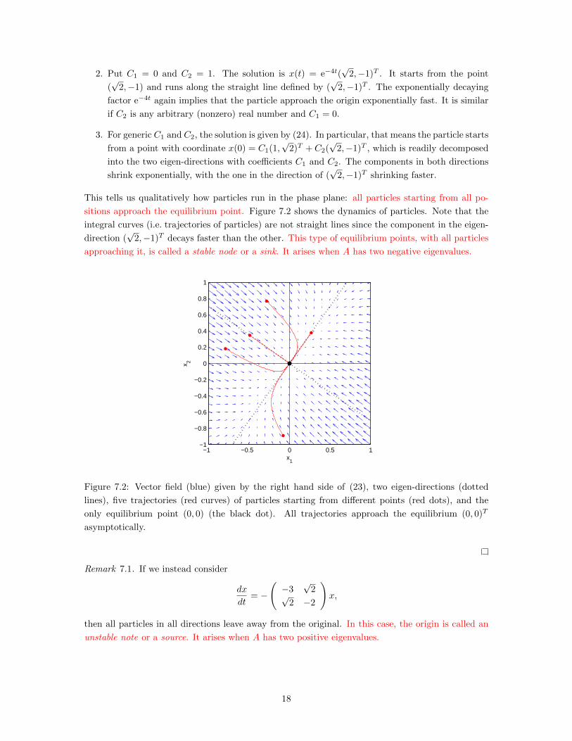
This tells us qualitatively how particles run in the phase plane: all particles starting from all po-

sitions approach the equilibrium point. Figure 7.2 shows the dynamics of particles. Note that the

integral curves (i.e. trajectories of particles) are not straight lines since the component in the eigen-

direction (√

2,−1)T decays faster than the other. This type of equilibrium points, with all particles

approaching it, is called a stable node or a sink. It arises when A has two negative eigenvalues.

−1 −0.5 0 0.5 1−1

−0.8

−0.6

−0.4

−0.2

0

0.2

0.4

0.6

0.8

1

x1

x 2

Figure 7.2: Vector field (blue) given by the right hand side of (23), two eigen-directions (dotted

lines), five trajectories (red curves) of particles starting from different points (red dots), and the

only equilibrium point (0, 0) (the black dot). All trajectories approach the equilibrium (0, 0)T

asymptotically.

Remark 7.1. If we instead consider

dx

dt= −

(−3

√2√

2 −2

)x,

then all particles in all directions leave away from the original. In this case, the origin is called an

unstable note or a source. It arises when A has two positive eigenvalues.

18

7.2 Case II: two conjugate complex eigenvalues

The examples we have discussed so far all belong to the first case, i.e. the coefficient matrix A

has two distinct real eigenvalues. Now we shall see some examples of the second case, where the

matrix A has two distinct complex conjugate eigenvalues.


dx

dt=

(− 1

2 1

−1 − 12

)x. (25)


det(A− rI) = det

(− 1

2 − r 1

−1 − 12 − r

)=

(−1

2− r)2

+ 1 = r2 + r +5

4.

Hence, two eigenvalues of A are r1 = −1+2i2 and r2 = −1−2i

2 , which are conjugate. The corresponding

eigenvectors are

ξ(1) =

(1

i

), ξ(2) =

(1

−i

).

Note that ξ(1) and ξ(2) are conjugate as well. Hence, the general solution of (25) is

x(t) = C1

(1

i

)e

−1+2i2 t + C2

(1

−i

)e

−1−2i2 t, (26)

where C1 and C2 are constants. Since x(t) is a real solution, C1 and C2 actually have to be conjugate.

This will give the correct form of real general solutions x(t).

However, we shall use another approach. Recall that Theorem 5.4 states that real and imaginary

parts of a complex solution are both solutions. Since (1, i)T e−1+2i

2 t is a solution, we rewrite it as(1

i

)e

−1+2i2 t =

(1

i

)e−

12 t(cos t+ i sin t) = e−

12 t

[(cos t

− sin t

)+ i

(sin t

cos t

)]. (27)

Hence, e−12 t(cos t,− sin t)T and e−

12 t(sin t, cos t)T are real solutions of (25). It is easy to check that

they are linearly independent. Therefore, the general form of real solutions of (25) is

x(t) = C̃1e−12 t

(cos t

− sin t

)+ C̃2e−

12 t

(sin t

cos t

), (28)

where C̃1 and C̃2 are arbitrary real constants. Note that to this end we do not need to use the other

complex solution (1,−i)T e−1−2i

2 t to derive more real solutions. Indeed, the two complex solutions

are conjugate with each other, so taking their real and complex parts essentially give the same pair

of real solutions.

Now we shall do the phase plane analysis by looking at solutions starting from some particular

points.

1. Put C̃1 = 1 and C̃2 = 0 in (28). The solution is x(t) = e−12 t(cos t,− sin t)T starting from

(1, 0). We find that it is composed of an exponentially decaying factor e−12 t and a unit vector

in R2 which rotates clockwise (think about why). Therefore, the particle runs clockwise along

a spiral towards the origin; it will go around the origin for infinitely many times but never

touches it.

19

2. Put C̃1 = 0 and C̃2 = 1. The solution is x(t) = e−12 t(sin t, cos t)T starting from (0, 1). Again,

it could be shown that the particle will run clockwise along a spiral towards the origin as in

the previous case.

3. For generic C̃1 and C̃2, the same conclusion could be made.

This tells us qualitatively how particles run in the phase plane: all particles starting will run along

a spiral clockwise towards the origin. Figure 7.3 shows the dynamics of particles. This type of

equilibrium points, with all particles approaching it while rotating around it, is called a stable spiral

point. It arises when A has two conjugate complex eigenvalues whose real parts are negative. In

−1 −0.5 0 0.5 1−1

−0.8

−0.6

−0.4

−0.2

0

0.2

0.4

0.6

0.8

1

x1

x 2

Figure 7.3: Vector field (blue) given by the right hand side of (25), five trajectories (red curves) of

particles starting from different points (red dots), and the only equilibrium point (0, 0) (the black

dot). All trajectories go around the equilibrium (0, 0)T clockwise for infinitely many times and

asymptotically approach it.

a similar fashion, we can derive that when A has two conjugate complex eigenvalues with positive

real parts, the origin will be an unstable spiral point. In this case, all particles will run along some

spirals and leave the origin.

Example 7.4 (This was left as an exercise in the recitation). Find general solutions of

dx

dt=

(0 −1

1 0

)x. (29)

Solution. Again we calculate all the eigen-pairs of A. We can find

det(A− rI) = r2 + 1.

Hence, two eigenvalues of A are r1 = i and r2 = −i. The corresponding eigenvectors are

ξ(1) =

(1

−i

), ξ(2) =

(1

i

).

20

Again, using Theorem 5.4, we rewrite

ξ(1)er1t =

(1

−i

)eit =

(1

−i

)(cos t+ i sin t) =

(cos t

sin t

)+ i

(sin t

− cos t

). (30)

Hence, (cos t, sin t)T and (sin t,− cos t)T are real solutions of (29). Therefore, the general form of

real solutions of (29) is

x(t) = C1

(cos t

sin t

)+ C2

(sin t

− cos t

), (31)

where C1 and C2 are arbitrary real constants.

It is not difficult to see that all trajectories, except the one starting from the origin, are concentric

circles centered at the origin; and all particles go along these circles counter-clockwise. Figure 7.4

shows the dynamics of particles. This type of equilibrium points, with all particles going around

it in some closed orbits, is called a center. It arises when A has two conjugate purely imaginary

eigenvalues. This is an example that an equilibrium point can be stable but not asymptotically

stable.

−1 −0.5 0 0.5 1−1

−0.8

−0.6

−0.4

−0.2

0

0.2

0.4

0.6

0.8

1

x1

x 2



dot). All trajectories go around the equilibrium (0, 0)T counter-clockwise along concentric circles.

This is an example in which the origin is stable but not asymptotically stable.

7.3 Case III: repeated real eigenvalues

Now we come to the last case where A has a real eigenvalue with multiplicity 2. If there are two

linearly independent eigenvectors corresponding to the eigenvalue, we can find out the solution and

do phase plane analysis as in Example 7.2. However, it is not always possible to find two linearly

independent eigenvectors, as is shown in the next Example.

21

Example 7.5. Find general solutions of

dx

dt=

(2 1

0 2

)x. (32)

Solution. We calculate all the eigen-pairs of A. Since det(A− rI) = (r− 2)2, A has an eigenvalue 2

with multiplicity 2. Then we look for its eigenvectors by solving for nonzero solution of(2− 2 1

0 2− 2

)ξ =

(0 1

0 0

)ξ = 0.

Only one solution ξ(1) = (1, 0)T could be found up to a scalar multiplication. That means, we are

not able to write down general solutions as before. So we need some new approach.

Note that with x = (x1, x2)T , (32) can be rewritten as

dx1dt

= 2x1 + x2, (33)

dx2dt

= 2x2. (34)

From the second equation, we derive that x2(t) = C2e2t. Plugging this into the first equation and

solving that (think about how), we obtain that x1(t) = C1e2t+C2te2t. Therefore, we find the general

solution of (32)

x(t) = C1e2t

(1

0

)+ C2e2t

(t

1

), (35)

where C1 and C2 are arbitrary real constants. To analyze the dynamics of particles, we note that

the factor e2t makes particles leave the origin. At the same time, the red t in (35) adds a drift in

the x1-direction. Particles in the upper half plane feel the drift to the right; while those in the lower

half plane can feel the drift to the left. Therefore, we are able to characterize the phase portrait

qualitatively. The phase portrait is shown in Figure 7.5. This type of equilibrium points is called

an unstable node although its behavior is slightly different from what we have seen before. It arises

when A has repeated real eigenvalues but only one eigenvector.

7.4 Summary (not covered in the recitation)

From the above example, we learn that it is important to know whether A has real distinct

eigenvalues, complex conjugate eigenvalues, or repeated real eigenvalues. Moreover, to determine

the stability of the equilibrium points (0, 0), we also need to know signs of the real parts of the

eigenvalues — roughly speaking, positive real parts implies that particles are driven away from the

origin while negative real parts means trajectories will asymptotically approach the origin. The

information of eigenvalues can be derived from entries of A. Recall that we have assumed that

A =

(a b

c d

), p = a+ d, q = ad− bc, ∆ = p2 − 4q.

Suppose A has two eigenvalues r1 and r2. Then

p = r1 + r2, q = r1r2, ∆ = (r1 − r2)2.

We summarize all the cases in Table 1. Alternatively, one can consult the following graph on

22

−1 −0.5 0 0.5 1−1

−0.8

−0.6

−0.4

−0.2

0

0.2

0.4

0.6

0.8

1

x1

x 2



dot). All trajectories go away from (0, 0)T with a horizontal drift.

Wikipedia https://en.wikipedia.org/wiki/Phase_plane#/media/File:Phase_plane_nodes.svg.

It has a minor mistake in the case of ∆ = 0 since it is possible that there are two linearly indepen-

dent eigenvectors so that the origin can be a node like the one in Example 7.2 instead of the one in

Example 7.5.

7.5 What is the relation between calculating etA and the approach used

here? (not covered in the recitation)

It seems that we are using a quite different approach from the one introduced in class to solve

and analyze the ODE systems. Recall that in the class, we learn that it suffices to calculate etA,

which is defined by a matrix power series. However, these two approaches are essentially equivalent.

We shall explain this in details in this section by recovering the matrix exponential method from

our approach in the recitation.

First suppose the 2 × 2-real matrix A is diagonalizable. To be more precise, there exists a

nonsingular 2×2-complex matrix P = (ξ1, ξ2), where ξ1 and ξ2 are columns of P , such that for some

r1, r2 ∈ C,

P−1AP =

(r1

r2

), Λ. (36)

This implies that

A(ξ1, ξ2) = (ξ1, ξ2)

(r1

r2

), (37)

i.e. Aξi = riξi. Hence, (ri, ξi) (i = 1, 2) are eigen-pairs of A. This implies that the general solution

can be written as

x(t) = C1er1tξ1 + C2er2tξ2 = P

(er1t

er2t

)(C1

C2

),

23

https://en.wikipedia.org/wiki/Phase_plane#/media/File:Phase_plane_nodes.svg

Table 1: Summary of all possible cases of linear 2× 2-real ODE systems

∆ p q Eigenvalues r1, r2 of A Type of the origin

∆ > 0 p > 0 q > 0 r1, r2 > 0, r1 6= r2 unstable node (Example 7.2)

p < 0 q > 0 r1, r2 < 0, r1 6= r2 stable node (Example 7.2)

p = 0 q ≥ 0 - -

p ∈ R\{0} q = 0 one is 0; one is p degenerate case (not covered)

p ∈ R q < 0 one is positive; one is negative saddle point (Example 7.1)

∆ < 0 p > 0 q > 0 r1, r2 ∈ C, r̄1 = r2, Re ri > 0 unstable spiral (Example 7.3)

p = 0 q > 0 r1, r2 ∈ C, r̄1 = r2, Re ri = 0 center (Example 7.4)

p < 0 q > 0 r1, r2 ∈ C, r̄1 = r2, Re ri < 0 stable spiral (Example 7.3)

p ∈ R q ≤ 0 - -

∆ = 0 p > 0 q > 0 r1 = r2 > 0 unstable node (Example 7.2, 7.5)

p < 0 q > 0 r1 = r2 < 0 stable node (Example 7.2, 7.5)

p = 0 q = 0 r1 = r2 = 0 degenerate case (not covered)

p = 0 q 6= 0 - -

p ∈ R\{0} q ≤ 0 - -

Here “-” means this case is not possible. For the case ∆ = 0, one needs to determine if there are two

linearly independent eigenvectors. If there are, analyze the system as in Example 7.2; otherwise, do

the analysis as in Example 7.5.

with the initial data

x0 = x(0) = P

(C1

C2

).

Therefore,

x(t) = P

(er1t

er2t

)P−1x0. (38)

Now we would like to ask whether or not a generic 2 × 2-real matrix A is diagonalizable as in

(36). The answer is no; assuming Λ to be diagonal is too strong and is not always achievable. We

can only assume Λ is the Jordan canonical form of A, which is a block diagonal matrix with each

block being a Jordan block of the following form

J(r,m) =

r 1

r 1. . .

. . .

r 1

r

m×m

. (39)

When A has two distinct eigenvalues, the Jordan blocks that form Λ can only be of size 1. Hence, Λ

is a diagonal matrix and A is diagonalizable. When A has repeated eigenvalues, the Jordan blocks

that form Λ can be of size 1 or 2. In the former case, A is also diagonalizable, corresponding to the

case when A has repeated eigenvalues together with two linearly independent eigenvectors. In the

24

latter case when Λ is a 2-Jordan block, the equation (18) reduces to

d(P−1x)

dt=

(r 1

0 r

)P−1x. (40)

Following the same derivation in Example 7.5, we can solve the equation for (P−1x),

P−1x(t) = C1ert

(1

0

)+ C2ert

(t

1

)= ert

(1 t

0 1

)(C1

C2

)=

(ert tert

0 ert

)(P−1x)(0).

(41)

Here C1 and C2 are determined by initial data at t = 0. Therefore,

x(t) = P

(ert tert

0 ert

)P−1x(0). (42)

Now it suffices to check that

A = P

(r1 0

0 r2

)P−1 ⇒ etA = P

(er1t 0

0 er2t

)P−1, (43)

and

A = P

(r 1

0 r

)P−1 ⇒ etA = P

(ert tert

0 ert

)P−1. (44)

We leave it to readers.

The above argument treats the matrix exponential as something which we define to be what we

have found out (the form of solutions we obtained above). However, it is not the case. It should be

clear that the definition of the matrix exponential comes first, which is natural and intrinsic. We

will not discuss it here though, since it is far beyond the scope of this class.

References

[1] E.A. Coddington, An Introduction to Ordinary Differential Equations (corrected edition, Dover,

1989).

[2] W.E. Boyce and R.C. DiPrima, Elementary Differential Equations and Boundary-Value Prob-

lems (10th edition, Wiley, 2012).

[3] Lawrence Perko. Differential equations and dynamical systems (Vol. 7. Springer Science & Busi-

ness Media, 2013).

25

Notes of ODE Recitations - NYU Courant · Notes of ODE Recitations Jiajun Tong October 29, 2016 1...

Documents

Transcript of Notes of ODE Recitations - NYU Courant · Notes of ODE Recitations Jiajun Tong October 29, 2016 1...