Notes for ’Hydrogeology’ - Anders Damsgaard · Notes for ’Hydrogeology’ Anders Damsgaard...

Notes for ’Hydrogeology’

Anders Damsgaard Christensen - [email protected]

Last revision: January 26, 2010Version 0.4

About this compendium

This document is created on base of the lectures in the course ’Hydrogeology’ held byKeld Rømer Rasmussen at the department of Geology at Århus University, that I followedduring the fall semester 2009. All figures and tables are recreated and possibly modifiedwithout permission, and this document is strictly for personal use only. Redistribution isnot allowed. I cannot be held responsible regarding the correctness of factual claims madein this document.

This document is created with LATEX

Contents

1 Introduction 7

1.1 Lecture material . . . . . . . . . . . . . . . . . . . . . . . . . . . . . . . . . 7

1.2 Main topics . . . . . . . . . . . . . . . . . . . . . . . . . . . . . . . . . . . 7

2 Geometric elements of open channels 9

3 Fundamentals 10

3.1 Flow . . . . . . . . . . . . . . . . . . . . . . . . . . . . . . . . . . . . . . . 10

3.1.1 Rectangular channel . . . . . . . . . . . . . . . . . . . . . . . . . . 10

3.1.2 Trapezoidal-, Triangular- and circular channels . . . . . . . . . . . . 11

3.1.3 Stationary flow, steady flow . . . . . . . . . . . . . . . . . . . . . . 11

3.2 Discharge . . . . . . . . . . . . . . . . . . . . . . . . . . . . . . . . . . . . 11

4 Energy and momentum principles 12

4.1 Hydrostatic pressure distribution . . . . . . . . . . . . . . . . . . . . . . . 12

4.2 Ideal fluids . . . . . . . . . . . . . . . . . . . . . . . . . . . . . . . . . . . . 13

4.3 Real fluids . . . . . . . . . . . . . . . . . . . . . . . . . . . . . . . . . . . . 13

4.4 Open channel flow classification . . . . . . . . . . . . . . . . . . . . . . . . 14

2

Hydrogeology CONTENTS

4.5 Mass transfer . . . . . . . . . . . . . . . . . . . . . . . . . . . . . . . . . . 14

4.6 Momentum transfer . . . . . . . . . . . . . . . . . . . . . . . . . . . . . . . 14

4.7 Energy transfer . . . . . . . . . . . . . . . . . . . . . . . . . . . . . . . . . 15

4.8 Conservation of mass . . . . . . . . . . . . . . . . . . . . . . . . . . . . . . 15

5 Critical flow 17

5.1 Head expression . . . . . . . . . . . . . . . . . . . . . . . . . . . . . . . . . 17

5.2 Froudes number . . . . . . . . . . . . . . . . . . . . . . . . . . . . . . . . . 18

5.2.1 Critical depth . . . . . . . . . . . . . . . . . . . . . . . . . . . . . . 18

5.2.2 Specific energy - E . . . . . . . . . . . . . . . . . . . . . . . . . . . 18

5.2.3 Small threshold at the stream bottom (Q constant) . . . . . . . . . 19

5.2.4 Choking . . . . . . . . . . . . . . . . . . . . . . . . . . . . . . . . . 19

6 Friction in fluids 20

6.1 Reynolds number . . . . . . . . . . . . . . . . . . . . . . . . . . . . . . . . 21

6.2 Mannings approximation . . . . . . . . . . . . . . . . . . . . . . . . . . . . 21

6.3 Single loss (enkelttab) . . . . . . . . . . . . . . . . . . . . . . . . . . . . . 22

6.4 Loss in pipes with turbulent flow . . . . . . . . . . . . . . . . . . . . . . . 23

6.5 Composite channels . . . . . . . . . . . . . . . . . . . . . . . . . . . . . . . 23

6.6 Compound channels . . . . . . . . . . . . . . . . . . . . . . . . . . . . . . 24

7 Hydraulic structures 25

7.1 Broad crested weir (Bredt overløb) . . . . . . . . . . . . . . . . . . . . . . 25

7.1.1 Free and ventilated weirs - Generally . . . . . . . . . . . . . . . . . 26

7.2 Sharp-crested weir (Skarpkantet overloeb) . . . . . . . . . . . . . . . . . . 26

3


8 Open channel flow - Summary 28

8.1 Example - Aarhus stream . . . . . . . . . . . . . . . . . . . . . . . . . . . 28

8.2 Losses in hydraulic streams . . . . . . . . . . . . . . . . . . . . . . . . . . 28

8.2.1 Simple (turbulent?) system . . . . . . . . . . . . . . . . . . . . . . 28

8.2.2 Laminar flow . . . . . . . . . . . . . . . . . . . . . . . . . . . . . . 29

8.3 Drainage of groundwater aquifers . . . . . . . . . . . . . . . . . . . . . . . 29

9 Groundwater flow - basics 30

9.1 Poriosity of a soil . . . . . . . . . . . . . . . . . . . . . . . . . . . . . . . . 30

9.2 Hydraulic conductivity - Darcy’s experiment . . . . . . . . . . . . . . . . . 31

9.3 Refraction of streamlines (Brydningsloven) . . . . . . . . . . . . . . . . . . 32

9.4 Aquifer flow . . . . . . . . . . . . . . . . . . . . . . . . . . . . . . . . . . . 33

9.5 Confined aquifers . . . . . . . . . . . . . . . . . . . . . . . . . . . . . . . . 33

9.5.1 Derivation of the flow equation . . . . . . . . . . . . . . . . . . . . 33

9.6 Leakage aquifer . . . . . . . . . . . . . . . . . . . . . . . . . . . . . . . . . 35

9.7 Unconfined (phreatic / water table) aquifer . . . . . . . . . . . . . . . . . . 37

9.7.1 Linearizing the Boussinesque equation - Homogenous and isotropicaquifer . . . . . . . . . . . . . . . . . . . . . . . . . . . . . . . . . . 37

9.8 Defining the flow problem . . . . . . . . . . . . . . . . . . . . . . . . . . . 38

9.8.1 Interaction with the surroundings - Boundary value problems (BVP) 39

4


10 Analytical models 40

10.1 Steady state flow to a well in a leakage aquifer . . . . . . . . . . . . . . . . 40

10.2 Unsteady flow to wells . . . . . . . . . . . . . . . . . . . . . . . . . . . . . 42

10.2.1 Recovery test . . . . . . . . . . . . . . . . . . . . . . . . . . . . . . 42

10.2.2 Theis eq - Well function - Estimating T and S from type curve plot 43

10.2.3 Storage in confined aquifers . . . . . . . . . . . . . . . . . . . . . . 45

10.2.4 Barometer influences in confined aquifers . . . . . . . . . . . . . . . 46

10.3 Unsteady flow to wells in a confined aquifer . . . . . . . . . . . . . . . . . 46

10.3.1 Elasticity . . . . . . . . . . . . . . . . . . . . . . . . . . . . . . . . 46

10.3.2 Transient flow in a confined aquifer . . . . . . . . . . . . . . . . . . 46

10.4 Leaky aquifers . . . . . . . . . . . . . . . . . . . . . . . . . . . . . . . . . . 47

10.4.1 Leaky aquifer geometry . . . . . . . . . . . . . . . . . . . . . . . . . 47

10.4.2 Drawdown . . . . . . . . . . . . . . . . . . . . . . . . . . . . . . . . 48

10.4.3 Type curves . . . . . . . . . . . . . . . . . . . . . . . . . . . . . . . 49

10.5 Unconfined aquifers/Water table aquifers, S&Z ch.11 . . . . . . . . . . . . 49

10.5.1 Geometry . . . . . . . . . . . . . . . . . . . . . . . . . . . . . . . . 50

10.5.2 Pumping . . . . . . . . . . . . . . . . . . . . . . . . . . . . . . . . . 50

10.5.3 Drawdown and delayed storage, Neumann type curves . . . . . . . . 51

10.5.4 Early and late effects . . . . . . . . . . . . . . . . . . . . . . . . . . 51

10.5.5 Summary . . . . . . . . . . . . . . . . . . . . . . . . . . . . . . . . 52

10.6 Slug testing and stepwise testing, S&Z ch.12 . . . . . . . . . . . . . . . . . 53

10.7 Bounded aquifers . . . . . . . . . . . . . . . . . . . . . . . . . . . . . . . . 53

5


10.7.1 Drawdown near positive boundary . . . . . . . . . . . . . . . . . . . 54

10.7.2 Drawdown near negative boundary . . . . . . . . . . . . . . . . . . 56

10.7.3 Pumping situations with multiple positive/negative boundaries . . . 58

10.7.4 Well between two streams in infinite strip . . . . . . . . . . . . . . 58

10.8 Well in uniform flow . . . . . . . . . . . . . . . . . . . . . . . . . . . . . . 58

10.9 Abstraction - long term influences, S&Z ch.8 . . . . . . . . . . . . . . . . . 60

10.9.1 Release of water - initial phase . . . . . . . . . . . . . . . . . . . . . 62

10.9.2 Release of water - late phase . . . . . . . . . . . . . . . . . . . . . . 63

10.10Salt water intrusion . . . . . . . . . . . . . . . . . . . . . . . . . . . . . . . 63

10.11Stream groundwater interaction . . . . . . . . . . . . . . . . . . . . . . . . 64

A Hydrogeology terms 66

B Commonly used formulas 69

B.1 Basic hydraulics in streams . . . . . . . . . . . . . . . . . . . . . . . . . . . 69

B.2 Groundwater . . . . . . . . . . . . . . . . . . . . . . . . . . . . . . . . . . 70

B.2.1 W(u) - Theis equation/Well function . . . . . . . . . . . . . . . . . 71

B.2.2 Unconfined aquifer: Steady 1D groundwater flow . . . . . . . . . . 71

B.2.3 Confined aquifer: Steady 1D groundwater flow . . . . . . . . . . . . 71

B.2.4 Boundary conditions . . . . . . . . . . . . . . . . . . . . . . . . . . 72

6

Chapter 1

Introduction

Lectures Monday 9-11 (1525-229), and exercises Tuesday 8-10 (1525-229).Homepage: http://aula.au.dk/courses/HYDROE04/Mail: [email protected]

1.1 Lecture material

Osman Akan: Open Channel Hydraulics Chapters 1, 2, 3 and 6.

F.W. Schwartz and Hubao Zhang: Fundamentals of Ground Water Main book.

Jacob Bear: Hydraulics of Groundwater Two chapters

C.T. Jenkins: The influence from pumping near a stream

Keld Rasmussen: Exercises in hydrogeology

1.2 Main topics

• Basic hydraulics in streams

– Mannings formula

– Specific energy (diagrams, Froude’s number)

– Linear reservoirs

• Groundwater

7

Hydrogeology CHAPTER 1. INTRODUCTION

– Confined aquifers

– Watertable aquifers (often treated as confined aquifers)

– Leakage aquifers (steady state when leakage in cone equals the pumping rate)

– Finding hydraulic parameters by simple pumping tests

∗ Cooper-Jacob plot∗ Theis plot∗ Delayed storage

– Streams: Assume that there is no loss at the groundwater-stream interface.Streams are a positive or negative boundary.

8

Chapter 2

Geometric elements of open channels

Table 2.1: Relationship between various section elements

y Flow depth Vertical distance from the channel bottom to the freesurface

d Depth of flow section Flow depth measured perpendicular to the channel bot-tom. The relationship between d and y is d = y · cosθ.For most man-made and natural channels cosθ ≈ 1.0,and therefore y ≈ d.

T Top width Width of the channel section at free surface.P Wetted perimeter Length of the interface between the water-channel

boundary.A Flow area Cross-sectional area of the flow.D Hydraulic depth Flow area divided by top width: D = A/TR Hydraulic radius Flow area divided by wetted perimeter, R = A/PăS0 Bottom slope Longitudinal slope of the channel bottom, S0 = tanθ ≈

sinθ.γ Specific gravity γ = ρ · g

9

Chapter 3

Fundamentals

Textbook: Akan Ch.1

Three types of aquifers: Confined, leaky and phreatic (unconfined or water table aquifer).

3.1 Flow

Vector. Flow through a channel is conversion of potential energy to kinetic energy. Therestriction is friction.

3.1.1 Rectangular channel

Width: b, Depth: y

The area of the flow: A = by , [m2]

Wetted perimeter: P = b+ 2y , [m]

Hydraulic radius: how big the area of the flow is in relation to the wetted perimeter:

R(m) =by

b+ 2y

10

Hydrogeology 3.2. DISCHARGE

3.1.2 Trapezoidal-, Triangular- and circular channels

Akan, table 1.1.

Circular channels: Ex.: partially filled tube. A partially filled tube is better for trans-porting water than a completely filled tube.Akan, table 1.1.

3.1.3 Stationary flow, steady flow

Flow is said to be steady if the flow conditions do not vary in time. Therefore, the partialderivative terms with respect to time can be dropped from the continuity, momentum andenergy equations.

3.2 Discharge

dQ = ~v · d ~A

For a large cross section with area A: V̄ = QA

In a channel there is a continuity, that requires inverse behavior of area and velocity. I.e.in a larger channel the velocity of the stream is lower than in a narrower section.

11

Chapter 4

Energy and momentum principles

4.1 Hydrostatic pressure distribution

Piezometric head (Trykniveau):

z +p

γ= h = constant

Valid in open water bodies and open (non-confined) groundwater aquifers, where flowis parallel to the surface and bottom. That means the pressure is the same value in ahorizontal plane.

When we look at pressure, we look at a static fluid. The surface is integrated over thevertical section.

Force perpendicular to the vertical surface: Fp =∫γydA

Definition of centroid (tyngepunkt): Yc =∫

ydAA

So that: Fp = γYcA

The pressure force is always acting slightly below the centroid.

The pressure at the bottom of a stream is the overlying weight of the fluid. If thestream/tube is oriented vertical, no pressure is applied at the sides. The pressure de-creases with an increasing inclination (hældning).

12

Hydrogeology 4.2. IDEAL FLUIDS

4.2 Ideal fluids

1. Frictionless, i.e. viscosity µ = 0.

2. No loss of energy when flowing.

3. No eddies (hvirvler) will develop because of friction.

Bernoulli’s equation applies: p+ 12· ρv2 + γz = constant, which consists of internal energy

+ kinetic energy + potential energy = constant.

Rewrites to: z + pγ

+ v2

2g= constant

When observing ground water elevation, the height (h) of the groundwater table is a goodexpression for the energy, because the velocity is relatively very small, and the pressure atthe groundwater table equals atmospheric pressure.

Se slide "Example: Container with a short, streamlined nozzle", for using Bernoulli’sequation. The potential energy at position A is converted to kinetic energy at position B.

The result is Toricellis theorem (when the friction is ignored), that gives the velocity ofthe escaping water at a height: v0 =

√2gh

4.3 Real fluids

When there is a loss of energy due to friction and surface tension, so a velocity coefficientis introduced: v0 = Cv

√2gh, where Cv ≈ 0.95− 0.99.

Real fluids have viscosity µ. x1 is the horizontal axis, x2 is the vertical axis.

For laminar flow of Newtonian fluids:

τ = µ

(δv1

δx2

+δv2

δx1

)For a laminar planar flow - Newtons formula:

τ = µδv1

δx2

The velocity of the water molecules is zero (0) at the bottom/wall/side. The velocity risesconstantly with the distance from the wall/bottom/side.

Groundwater flows with planar flow because of small pipe radius and slow water movementspeeds.

13

Hydrogeology CHAPTER 4. ENERGY AND MOMENTUM PRINCIPLES

4.4 Open channel flow classification

Laminar or turbulent flow? Determined by the ratio of inertial forces to viscous forces.Reynold’s number (Re) is dimensionless.

Re =V R

νNumerical boundaries depend on the choice of variables. ν: kinematic viscosity, V : averagevelocity, R: hydraulic radius. 580 ≤ Re ≤ 750. Laminar flow beneath 580, turbulent above750.

A rule of thumb: Groundwater flow laminar, surface flow turbulent.

Ratio of inertial forces to gravity (Froude’s number small or large):

Fr =V√gD

Fr < 1 : SubcriticalFr = 1 : CriticalFr > 1 : Supercritical

Large rivers with calm surface are in a subcritical state. Mountain streams with waves ontop are supercritical.With the same discharge (Q) the water can flow slowly through a large area (subcritical),or fast through a small area (supercritical). This is related to the inclination to the bed.

4.5 Mass transfer

Discharge is Q. Mass (M) transfer for an incompressible fluid in an open channel (pipe)flow is called the mass flux or the mass transfer rate.

Rate of mass transfer = Mass flux = ρQ

4.6 Momentum transfer

Momentum is a property of a moving object: p = M · V

Momentum is the numerical measure of an objects tendency to keep moving in the samemanner.

Mass flux at any point: φM = ρdQ = ρvdA.

Momentum flux at any point: φp = v · ρdQ

14

Hydrogeology 4.7. ENERGY TRANSFER

4.7 Energy transfer

The total energy (internal + kinetic + potential) is converted to a size of potential energy,E = [m]. The potential energy is a relative quantity to a reference elevation.

The potential energy of an object of mass M isMgzc, where g = gravitational acceleration,zc = elevation of the center of mass above the reference level.In open channel flow: Q = discharge (rate of volume transfer), and ρQ = rate of masstransfer.

Therefore, the rate of potential energy transfer through a channel section:

Rate of potential energy transfer = Ep = ρQgzc

Rate of kinetic energy transfer (v: point velocity):

Ek =1

2· ρvdA · v2 =

ρ

2

∫A

v3dA

In practice, it is easier to use the average cross-sectional velocity, V. α: energy coefficientor kinetic energy correction coefficient:

Ek = αρ

2V 3A = α

ρ

2QV 2

α = 1 (for rectangular channels)

α =

∫Av3dA

V 3A

Rate of internal energy transfer:

Ep = ρeV A = ρevdA = ρeQ

4.8 Conservation of mass

Consider a volume element of an open channel between upstream section U and downstreamsection D, with length ∆x, and average cross-sectional area A.The mass of water present in the volume: ρA∆x

Water enters at upstream section at a mass transfer rate: ρQU , and leaves at downstreamsection at a rate ρQD.Change in the elements volume over time increment ∆t: ∆(ρA∆x)

∆t

15

Hydrogeology CHAPTER 4. ENERGY AND MOMENTUM PRINCIPLES

The difference in water volumes that enters and leaves the volume elementmust equal the change in the elements volume.

ρQU − ρQD =∆(ρA∆x)

∆t

For a gradually-varied flow A and Q are continuous in space and time, and as ∆x and ∆tapproach zero, the equation becomes....:

δA

δt+δQ

δx= 0

....the continuity equation!

16

Chapter 5

Critical flow

Textbook: Akan Ch. 2 cont.

5.1 Head expression

From the energy equation:

H = zbU + yU +αUV

2U

2g= zbD + yD +

αDV2D

2g+ ∆H

∆H is the head loss of energy between the two boundaries: U upstream and D downstream.

zb : Elevation head, [m] (or [ft])yU : Pressure head, [m]H : Total energy headαUV

2U

2g: Velocity head

For groundwater where the velocity is low, the piezometric head or hydraulic head:

h = zb + y

17

Hydrogeology CHAPTER 5. CRITICAL FLOW

5.2 Froudes number

DimensionlessF =

V√gD

Subcritical flow: F < 1 : Surface waves can move up-streamSupercritical flow: F > 1 : Surface waves cannot move up-streamCritical flow: F = 1

5.2.1 Critical depth

The depth where the flow is critical (F = 1). For a rectangular channel (other types inAkan):

yc = 3

√q2

g

q : Specific flow rate (discharge per meter across the stream), [m3

sm−1 = m2

s]

The critical flow happens at one section in the elevation (not over a distance along theflow). With critical flow, the specific energy has its minimal value (Emin).

At constant energy (E) and constant discharge (Q), the flow can exist in two forms (twoy-values), i.e. in either supercritical or subcritical form.

That is, either subcritical with large depth (y), or in supercritical state with small depth(y).

Critical flow is where a maximum in flow can happen at a minimum in energy (Emin).

5.2.2 Specific energy - E

E ≈ y +αQ2

2gA2

Velocity coefficient α is usually 1.

18

Hydrogeology 5.2. FROUDES NUMBER

5.2.3 Small threshold at the stream bottom (Q constant)

Energy loss at positive structure.

a) Subcritical flow:Stream depth decreases over threshold.

b) Supercritical flow:Stream depth increases over threshold.

E decreases with ∆z. E decreases, so stream depth y changes corresponding to Figure2.11, Akan.

5.2.4 Choking

If the threshold is so high, that the energy is too low in the stream to pass it with theconstant discharge Q (→ moving left of Emin in fig. 2.11, Akan), the water level y will rise,until at least Emin is reached over the threshold.The discharge Q will reduce, until the necessary y is developed in front of the threshold.

19

Chapter 6

Friction in fluids

Textbook: Akan, ch. 3

A wall: Boundary where the flow velocity equals zero (0), (No slip conditions).This creates a velocity gradient: An area with increasing flow velocities. This zone is calledthe boundary layer. The atmospheric boundary layer has about 1 km thickness from thesurface.

Near the boundary: Stress and friction.

Flows can be completely laminar, turbulent with a laminar wall layer or fully turbulent.

Sf : Friction lossτ0: Friction force per unit area (no matter flow type)

τ0 = γRS0 where:R = A/P : Hydraulic radiusS0: Slope of the bedγ = ρg: Specific gravity

Insert notes about pipe resistance and Darcy-Weisbach number from Slides + Akan.

Fraction of kinetic energy, where f is the Darcy-Weisbach number:

τ0 = f · 1

2ρV 2

The Darcy-Weisbach number is a function of Reynolds number, form and roughness. TheReynolds number is a function of speed. ks = k: The particle diameter of a spheric grain.

20

Hydrogeology 6.1. REYNOLDS NUMBER

• Laminar flow:f =

64

Re

• Smooth flow (Re < 100.000):

f =0.316

Re0.25

• Fully rough turbulent flow:1√f

= −2logks

12R

6.1 Reynolds number

Re =V R

ν

u∗ = us =

√τ0

ρ

ν is the viscosity.

6.2 Mannings approximation

Walls in nature are rough.

• For rough cylindrical pipes:√2

f=V

u∗= 6.62 + 2.45ln

(R

k

)• For rough rectangular pipes:√

2

f=V

u∗= 6.15 + 2.45ln

(R

k

)• For rough pipes: √

2

f=V

u∗= 6.40 + 2.45ln

(R

k

)

21

Hydrogeology CHAPTER 6. FRICTION IN FLUIDS

In nature (Manning):

4.7 <R

k< 300

u∗ =√gRS0

⇒ V

u∗≈ 8.1

(R

k

)1/6

⇒ V ≈ 8.1

(R

k

)1/6

·√gRS0

M =25.4

6√k

m1/3s−1 (Manning number)

⇒ V = M ·R2/3 · S1/20 =

knn·R2/3 · S1/2

0

⇒ Q = AV

The n-value is the Manning factor, used in the imperial system. Mannings number (M)can be found in tables. Often: 10 < M < 40.

6.3 Single loss (enkelttab)

Expansion carnot, where flow is moving from a small pipe into a larger one. Loss of partof the kinetic energy (αA = 1.1):

∆HE = αA(VA − VB)2

2g

Flow into large reservoir; loss of the entire kinetic energy:

∆HE = αV 2

2g

Generally:

∆HE = ξ(VA − VB)2

2g

For a sudden, sharp contraction: ξ = 0.5For a smoothened contraction (bottleneck type): ξ = 0.1For a gradual contraction: ξ = 0

Bends:

ξ = 1.1

(θ

90

)2

22

Hydrogeology 6.4. LOSS IN PIPES WITH TURBULENT FLOW

6.4 Loss in pipes with turbulent flow

The losses in the different parts of the system are summed together:

• Inlet loss:∆HI = 0.5

Q2

2gA2

• Pipe loss (friction):

∆HF =L

M2R4/3A2·Q

• Outflow loss:∆Hu =

αQ2

2gA2

• Total loss: ∑i

∆Hi = Q2

[∑ L

M2R4/3A2+∑ ξ

2gA2

]⇒∑i

∆Hi = H = k ·Q2

⇒ Q =

√H

k

k: Specific resistivity

In a pipe system, the section in the brackets in the upper formula is a constant. Whenplotting Q2(h), the result will be a straight line.

In natural channels, the hydraulic radius (R) may vary. The result is that the Q2(h) plotwill curve upwards in the ends.

6.5 Composite channels

Channels that have different roughness in different parts of the cross section (Fig 3.9,Akan). The equivalent roughness of the channel (ne, Manning koefficient):

ne =

[∑Ni=1(Pin

2i )∑N

i=1 Pi

]1/2

23

Hydrogeology CHAPTER 6. FRICTION IN FLUIDS

6.6 Compound channels

Channels that overflood during high discharges (Fig 3.10, 3.11, Akan).ă

The flow is divided into subsections. The conveyance (K) for each subsection:

Ki =knnAiR

2/3i

If the energy head is the same for all subsections:

Q =(∑

Ki

)S

1/20

24

Chapter 7

Hydraulic structures

Textbook: Akan, ch. 6

Hydraulic structures are often constructed for measuring the discharge via the water level(h) in higher resolution.

7.1 Broad crested weir (Bredt overløb)

Fig 6.7, Akan. On the broad crested weir, the flow transfers from upstream subcritical flowinto critical flow on top of the weir, and exits as a jet with surrounding air in supercriticalstate (nappe).

E =3

2yc =

3

23

√αq2

g⇒ q =

√4

27αH√

2gH =2

3√

3H√

2gH

h ≈ H;α ≈ 1⇒ q = 0.38h√

2gh ≈ 1.7h3/2

C0 =2

3√

3

The above relationship between specific discharge (q) and water level (h) can be calibratedvia measurements.

Geometric and hydraulic elements: w: Weir height, Q: Discharge, q: Specific discharge, h:Flow height upstream over weir, H: energy upstream (h < H), yc: Critical depth, b: Weirwidth.

25

Hydrogeology CHAPTER 7. HYDRAULIC STRUCTURES

7.1.1 Free and ventilated weirs - Generally

(As example above)Q = C0bH

√2gH

If the upstream velocity is significant:

Q = Cbh√

2gH ⇒ C 6= C0

C = C0

[1 +

αq2

2g(w + h)2h

]3/2

7.2 Sharp-crested weir (Skarpkantet overloeb)

Usage of the energy equation to obtain a relationship between the approach flow charac-teristics and the discharge over a weir. Rectangular sharp crested weir:

Q = kwLew√

2gh3/2e0 (6.4)

Correction factors. Effective head over crest:

he0 = h0 + hk , hk = 0.001m

The effective crest length:Lew = Lw + Lk

26

Hydrogeology 7.2. SHARP-CRESTED WEIR (SKARPKANTET OVERLOEB)

27

Chapter 8

Open channel flow - Summary

Different contributions for open channel water:

• Precipitation

• Ditches

• Groundwater flow

• Drains and other man-made structures

8.1 Example - Aarhus stream

Discharge highest in winter.During summer: Generally speaking; Evapotranspiration > precipitation ⇒ Stream watersupplied by groundwater contribution.

During summer rainfalls, the precipitation will temporary infiltrate the aquifers as ground-water, until reentering the atmosphere into streams.

8.2 Losses in hydraulic streams

8.2.1 Simple (turbulent?) system

Quadratic relationship between energy differences and discharge:√h =

√h(t = 0)−Kt ⇒ ∆H ∝ Q2

28

Hydrogeology 8.3. DRAINAGE OF GROUNDWATER AQUIFERS

8.2.2 Laminar flow

Linear relationship between energy differences and discharge:

Q = KL∆H ⇒ ∆H ∝ Q

= −Adhdt⇒ h(t) = h0e

−Kt

This means, that the reservoir never empties.

8.3 Drainage of groundwater aquifers

Unconfined aquifer: Draining makes air replace water in upper lying pore-spaces, andthe groundwater-table drops.

Confined aquifer: Totally filled by water under pressure. The piezometric surface is thecorresponding water-pressure surface (groundwater-table in unconfined aquifer), observedin observation-drillings. Drainage lowers the pressure because of elastic storativity.

Lowering of the piezometric surface in a confined by drainage results in much less waterthan by lowering of the groundwater table in an unconfined aquifer.

29

Chapter 9

Groundwater flow - basics

Textbook: Schwartz & Zhang: Ch. 3, 4 (skip fractured rocks) and 5.1

Chapter 3 can be used as repetition for previously learned content.

9.1 Poriosity of a soil

The total porosity of a rock or soil is defined as the ratio of the void volume to the totalvolume of material:

nT =VvVT

=VT − VsVT

where nT is the total porosity, Vv is the volume of voids, Vs is the volume of solids and VTis the total volume. In some cases, porosity i expressed as percentage.

30

Hydrogeology 9.2. HYDRAULIC CONDUCTIVITY - DARCY’S EXPERIMENT

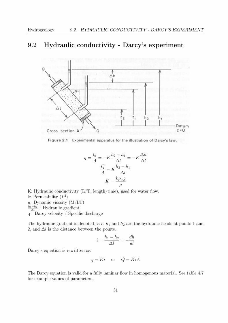
9.2 Hydraulic conductivity - Darcy’s experiment

q =Q

A= −Kh2 − h1

∆l= −K∆h

∆lQ

A= K

h2 − h1

∆l

K =kρwg

µ

K: Hydraulic conductivity (L/T, length/time), used for water flow.k: Permeability (L2)µ: Dynamic visosity (M/LT)h1−h2

∆l: Hydraulic gradient

q : Darcy velocity / Specific discharge

The hydraulic gradient is denoted as i. h1 and h2 are the hydraulic heads at points 1 and2, and ∆l is the distance between the points.

i =h1 − h2

∆l= −dh

dl

Darcy’s equation is rewritten as:

q = Ki or Q = KiA

The Darcy equation is valid for a fully laminar flow in homogenous material. See table 4.7for example values of parameters.

31

Hydrogeology CHAPTER 9. GROUNDWATER FLOW - BASICS

In the field, it is possible to install a large number of piezometers in a unit and to contourthe resulting head values. The gradient of change in head, and is maximal perpendicularto the lines of equal hydraulic head (equipotential lines).

9.3 Refraction of streamlines (Brydningsloven)

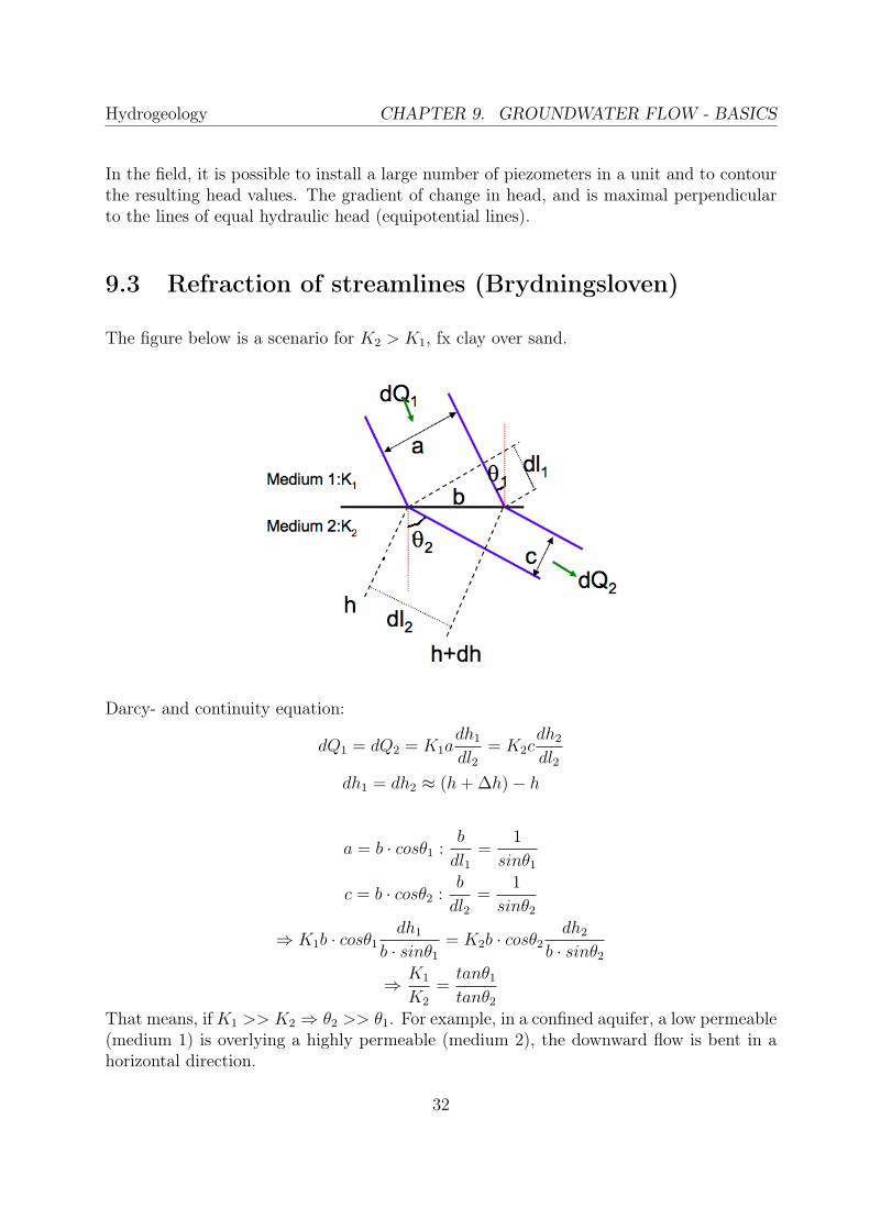
The figure below is a scenario for K2 > K1, fx clay over sand.

Darcy- and continuity equation:

dQ1 = dQ2 = K1adh1

dl2= K2c

dh2

dl2

dh1 = dh2 ≈ (h+ ∆h)− h

a = b · cosθ1 :b

dl1=

1

sinθ1

c = b · cosθ2 :b

dl2=

1

sinθ2

⇒ K1b · cosθ1dh1

b · sinθ1

= K2b · cosθ2dh2

b · sinθ2

⇒ K1

K2

=tanθ1

tanθ2

That means, ifK1 >> K2 ⇒ θ2 >> θ1. For example, in a confined aquifer, a low permeable(medium 1) is overlying a highly permeable (medium 2), the downward flow is bent in ahorizontal direction.

32

Hydrogeology 9.4. AQUIFER FLOW

9.4 Aquifer flow

The transmissivity describes the ease with which water can move through an aquifer.Transmissivity has units of [L2/T ].

T = Kb

K: Hydraulic conductivity, b (or B): Aquifer thickness

Aquifer flow can be considered horizontal. The length of a natural aquifer is muchgreater than its thickness. This means there is a small height-gradient, and as good ashorizontal flow.

Vertical flow is only relevant in proximity to well pumping and near springs and streams.

9.5 Confined aquifers

9.5.1 Derivation of the flow equation

Following principles are used: Conservation of mass, Darcy equation, Elastic propertiesand elastic laws.

In a compressible medium a volume change will result in a mass change within a controlmedium (changes in volume of porespaces). Conservation of flow volume (input -output = change of storage):

Qinflow −Qoutflow = Qstorage

Mass conservation[Mi −Mo] = ∆m/∆t

M = ρq , q : Specific discharge [m/s]

Left side (Mi −Mo). Same equations for x, y and z:

Mi,x = ρwqx∆y∆z (Inflow in x-direction)

Mo,x =

[ρwqx −

δ

δx(ρwqx)∆x)

]∆y∆z (Outflow in x-direction)

⇒ ∆M = −[δ

δx(ρwqx) +

δ

δy(ρwqy) +

δ

δz(ρwqz)

]∆z∆y∆x

∆M = −5 (ρw~q)VT = −div(ρw~q)VT

33


Right side (∆m/∆t). Poriosity is n. Mass of water in control box:

m = ρw · n ·∆x∆y∆z ⇒ δm

δt=

δ

δt(ρw · n)∆x∆y∆z

Combining left and right side, removing ∆x∆y∆z:

−[δ

δx(ρwqx) +

δ

δy(ρwqy) +

δ

δz(ρwqz)

]=δ(ρw · n)

δt

Assume that time changes in ρw override spatial changes:

−[δqxδx

+δqyδy

+δqzδz

]=

1

ρw

δ(ρw · n)

δt≡ Ss

δh

δt, [Ss] = m−1

Ss : Specific storativity. Delivery from 1m3 in reservoir per unit decline of head (h).δhδt

: Time-change of the hydraulic head.S : Storativity of the aquifer, S = Ss · B, assuming presence of hydrostatic pressuredistribution.B : Aquifer thickness

qi represents velocities, i.e. flow rate per cross section area. From the Darcy equation:

qi = −Kiδh

δxi[δ

δx

(Kx

δh

δx

)+

δ

δy

(Ky

δh

δy

)+

δ

δz

(Kz

δh

δz

)]= Ss

δh

δt

In isotropic aquifers or aquifer layers the hydraulic conductivity (K) is equal for flow in alldirections, while in anisotropic conditions it differs, notably in horizontal (Kh) and vertical(Kv) sense. In an isotropic, homogeneous medium: Kx = Ky = Kz = K

K

[δ2h

δx2+δ2h

δy2+δ2h

δz2

]= Ss

δh

δt

Steady flow (constant speed ( δhδt

= 0), fx regional settings):

δh

δt= 0⇒

[δ2h

δx2+δ2h

δy2+δ2h

δz2

]= 0 (Laplace equation)

Confined aquifer:[δ

δx

(Kx

δh

δx

)+

δ

δy

(Ky

δh

δy

)+

δ

δz

(Kz

δh

δz

)]= Ss

δh

δt

Now: T = KB and S = BSs , so we multiply with B on both sides and rewrite:[δ

δx

(Txδh

δx

)+

δ

δy

(Tyδh

δy

)]= S

δh

δt

34

Hydrogeology 9.6. LEAKAGE AQUIFER

Homogeneous and isotropic aquifer (isotropic: constant hydraulic conductivity):

δ2h

δx2+δ2h

δy2=S

T

δh

δt

1D flow:δ2h

δx2=S

T

δh

δt

9.6 Leakage aquifer

Basic equation for 2D flow. A leaky aquifer has an impermeable bed, an aquifier sectionon top (with parameters B,K), and a semi-permeable section over that (with parametersB’,K’). This material could be a till.

There is no significant horizontal flow in the semipermeable layer, but slow vertical down-ward flow (N), (scale: decimeters/year).

The sum of flow in the aquifer: Horizontal flow (incl. elastic component) + vertical supplyfrom semipermeable top layer (N).

Assumption: Time-constant watertable on top of semi-permeable layer.

Vertical (not horizontal!) head gradient in semipermeable layer (from Darcy eq):

φ0 − φB′

35


φ0 is the head of the upper watertable, and φ is the head at the bottom of the semipermeablelayer. B’ is the thickness. Instead of φ, h is used as the hydraulic head in the main aquifer.

Resulting downward supply to main aquifer from semipermeable layer:

N = K ′φ0 − hB′

=φ0 − hσ

, σ =B′

K ′

N: Downward flow into aquifer, B’: thickness of semipermeable layer, K’: Hydraulic con-ductivity of semipermeable layer, σ: Leakage coefficient.

Aquifer with 2D flow:[δ

δx

(Txδh

δx

)+

δ

δy

(Tyδh

δy

)]+N(x, y) = S

δh

δt

δ

δx

(Txδh

δx

)+

δ

δy

(Tyδh

δy

)+K ′

B′(φ0 − h) = S

δh

δt

Leakage factor: λ =√σT Homogenous, isotropic leaky aquifer (isotropic: constant hy-

draulic conductivity):δ2h

δx2+δ2h

δy2+

(φ0 − h)

λ2=S

T

δh

δt

1D flow:δ2h

δx2+

(φ0 − h)

λ2=S

T

δh

δt

36

Hydrogeology 9.7. UNCONFINED (PHREATIC / WATER TABLE) AQUIFER

9.7 Unconfined (phreatic / water table) aquifer

In the unconfined aquifer, the water table is the upper limit of the saturated zone. Thissurface is slightly sloping, and the flow is therefore not horizontal, see fig (a) below.

The flow has a vertical component, and therefore ds > dx. However, if θ ≤ 8o thencos > 0.99; so:

q = −Khdhds≈ −Khdh

dx

This means, that there is a non-linear (h2) relationship. These circumstances reflect figure(b) above, with vertical equipotential lines. This is called Dupuit’s approximation.

In the unconfined case Sy >> Ss, so both sides are multiplied with h.[δ

δx

(Kxh

δh

δx

)+

δ

δy

(Kyh

δh

δy

)]= [h · Ss + Sy]

δh

δt≈ Sy

δh

δt

In a homogenous and isotropic aquifer (Boussinesque equation):

δ

δx

(hδh

δx

)+

δ

δy

(hδh

δy

)=SyK

δh

δt

9.7.1 Linearizing the Boussinesque equation - Homogenous andisotropic aquifer

When H is large and variations in h are small, so that an average thickness of the aquifercan be introduced, i.e. h ∼ B:

δ

δx

(Bδh

δx

)+

δ

δy

(Bδh

δy

)=SyK

δh

δt⇒ δ2h

δx2+δ2h

δy2=

S

KB

δh

δt=S

T

δh

δt

37


Rewriting both sides using:

hδh

δt=

1

2

δ(h2)

δtand

S

K

δh

δt=S

K

1

2h

δ(h2)

δt

δ

δx

(hδh

δx

)+

δ

δy

(hδh

δy

)=SyK

δh

δt⇔ δ(h2)

δx2+δ(h2)

δy2=

SyKh

δ(h2)

δt≈ SyKB

δ(h2)

δt=SyT

δ(h2)

δt

1D flow:δ2(h2)

δx2=S

T

δ(h2)

δt

9.8 Defining the flow problem

• The governing flow equation (differential equation)

• Initial conditions

• Boundary conditions

The initial- and boundary conditions need to be known, in addition to the gorverning flowequation, to calculate the flow.

The flow is described by a partial differential equation (PDE) and the solution requiresdetermining:

• The geometry (x,y,z) of the flow domain must be known beforehand. The domainhas a bounding surface to a confining layer, or a curve F(x,y,z).

• The hydraulic parameters (K, Ss, B)

• The initial conditions (φ = φ1(x, y, z, 0))

• The interaction with the surroundings (boundary conditions)

Seek φ = φ(x, y, z, t) as the dependent variable.

38

Hydrogeology 9.8. DEFINING THE FLOW PROBLEM

9.8.1 Interaction with the surroundings - Boundary value prob-lems (BVP)

1. Known hydraulic head - Dirichlet BVP:φ = φ2(x, y, z, t) , example: a large lake, the sea.

2. Known flux - Neuman BVP:Example: Impermeable material → no flow at boundary: q = 0 and δh

δx= 0. See

textbook for formulas.

3. Semipermeably boundary (Mixed BVP) - Cauchy typeSee textbook for formulas

When there is a water table with recharge, the position and shape of the boundary condition(water table) is not known, but is part of the problem. ’Vicious circle argument’. Can leadto application of iterative methods in order to obtain a solution.

39

Chapter 10

Analytical models

Textbook: S&Z ch. 9

Insert missing notes f07.pdf

10.1 Steady state flow to a well in a leakage aquifer

Steady flow in an infinite aquifer is not possible. Flow into well:

Q(r) = qv +Q(r + ∆r)

qv is the vertical downward flow from the semi-permeable upper layer into the aquifer.Q(r + ∆r) is the horizontal flow from the surrounding aquifer. r is the distance from thewell, rw is well radius. Axis-symmentrical flow is assumed. Solution:

φ0 − φ(r) = αI0

( rλ

)+ βK0

( rλ

)I0: Modified Bessel function of first type and zero order.K0: Modified Bessel function of second type and zero order.K1: Modified Bessel function of second type and first order.

40

Hydrogeology10.1. STEADY STATE FLOW TO A WELL IN A LEAKAGE AQUIFER

If x << 1⇒ K0(x) ≈ ln(1,123x

)

If the leakage aquifer is unlimited:

x→∞⇒ I0(x)→∞, α = 0

⇒ φ0 − φ = βK0(r

λ

⇒ s = φ0 − φ =Q

2πT

K0[r/λ]

(rw/λ)K1[rw/λ]

Near the pumping well:

s(r) =Qw

2πT

41

Hydrogeology CHAPTER 10. ANALYTICAL MODELS

With increasing distance to the well, the lateral input decreases (Q(r)), and the verticaldownflow increases (qv).

Well function: ζ: Error’Distance with influence’ formula is a good approximation, no matter what u is.

10.2 Unsteady flow to wells

Notes from Bear-cont. (Hydraulics of Groundwater)S&Z: Ch 10Notes on Barometer curves

Investigating T and S of reservoirs by pumping tests.

10.2.1 Recovery test

Investigation methods: 1) Pumping for a limited time period, 2) Pumping (almost) con-tinuously in a water works.

Notes on above figure: y-axis: φ: Drawdown. The pumping takes place until t = tp = 500(Pumping rate: Qw). At t=500, t’ begins counting from zero. The recovery begins.

42

Hydrogeology 10.2. UNSTEADY FLOW TO WELLS

Mathematically this can be used. An equal size opposite discharge into aquifer is begun(−Qw) at pump shutdown.

t = tp + t′

s′(r, t) =Q

4πTlnt

t′=

Q

4πTlntp + t′

t′

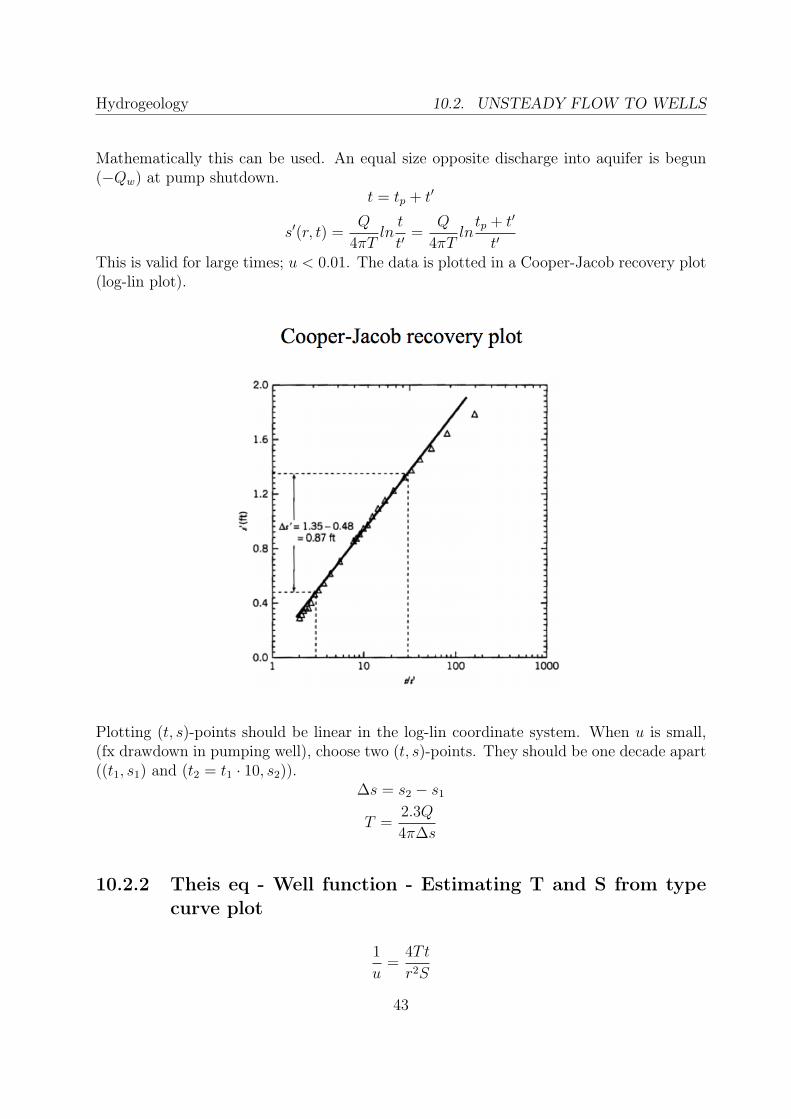
This is valid for large times; u < 0.01. The data is plotted in a Cooper-Jacob recovery plot(log-lin plot).

Plotting (t, s)-points should be linear in the log-lin coordinate system. When u is small,(fx drawdown in pumping well), choose two (t, s)-points. They should be one decade apart((t1, s1) and (t2 = t1 · 10, s2)).

∆s = s2 − s1

T =2.3Q

4π∆s

10.2.2 Theis eq - Well function - Estimating T and S from typecurve plot

1

u=

4Tt

r2S

43


S: Storativity, (not drawdown, s).

The Theis eq is plotted in a log-log plot (Well function), with x-axis: 1/u, y-axis: W(u)

Some drawdown (s,t) data is recorded in another well than the pumping well (observationalwell). The (s,t)-dataplot is put on top of the Well-function plot (typecurve). The twocurves are the same except for a displacement. The point (1,1) is used to calculate thedisplacement (figure below and the book uses another point).

44

Hydrogeology 10.2. UNSTEADY FLOW TO WELLS

T and S are found from the y- and x displacement. From y:

T =Q

4πs1

Where s1 is the drawdown for W (u) = 1. From x:

S = | tr2|14T = 1 · 4T

S =4Ttu

r2

10.2.3 Storage in confined aquifers

Once pumping is begun from a confined aquifer, a small influx (downward and upward)is flowing from the confining layers. This distorts the Theis curve. In this situation, adifferent type curve must be used, that accounts for the small storage in the confininglayers.

45


10.2.4 Barometer influences in confined aquifers

Normally: Pressure 0 (atmospheric) at watertable in an unconfined aquifer.

In a confined aquifer the piezometric surface is dependent on atmospheric pressure. Highatmospheric pressure ⇐⇒ Low piezometric level

Air pressure must be monitored when observation data is measured from a confined aquifer.As time goes on, the confined aquifer re compensates for the changed atmospheric pressure.

10.3 Unsteady flow to wells in a confined aquifer

10.3.1 Elasticity

The porous skeleton and the water is incompressible. In a confined aquifer the confiningupper layer is carried by granular stress (particle contact) and porewater pressure.

Elasticity modulus of water: β = δρw/δpρw

Elasticity modulus of skeleton (grains): α = δdz/δpdz

The expansion/contraction takes place along the vertical direction (up/down):

⇒ [α + nβ]gρwδh

δt≡ Ss

δh

δt

Ss: Storativity

10.3.2 Transient flow in a confined aquifer

Transient: Midlertidlig, kortvarig

Impermeable top + bottom. When pumping starts, a cone of depression is created inthe piezometric surface. With time, the cone expands out laterally. Water is supplied byelasticity.

u =r2S

4Tt

46

Hydrogeology 10.4. LEAKY AQUIFERS

s = φ0 − φ =Qw

4πTW (u)

W (u): Well function; exponential integrals: Drawdown at position r at time t.

The Well function:W (u) = −0.5772− ln(u) + ξ

where ξ → 0 for u→ 0 i.e. t→∞.

If u < 0.01:s =

Q

4πTln

2.25Tt

r2S=

2.303Q

4πTlog10

2.25Tt

r2S

The minimum distance for no influence from well at time t:

s =Q

4πTln

2.25Tt

r2S= 0

2.25Tt

r2S= 1⇒ r = 1.5

√Tt

S

10.4 Leaky aquifers

10.4.1 Leaky aquifer geometry

47


10.4.2 Drawdown

A: No leakage, Theis eq.B: Leakage, no storage in semipermeable layer (S ′s = 0)C: Leakage, and storage in semipermeable layer (S ′s 6= 0)

Confined aquifer with leakage. With existence of a constant head above semipermeablelayer:

δ2φ

δr2+

1

r

δφ

δr+φ0 − φλ2

=S

T

δφ

δt

Where φ0−φλ2 is the leakage component.

The drawdown:s(r, t) =

Q

4πTW (u, r/B) , u =

r2S

4Tt

B =√b′T/K ′: Leakage factor

Q: Amount of pumpingr: Distance from wellt: Timeb’: Thickness of the confining layerK’: Hydraulic conductivity of the confining layer

48

Hydrogeology10.5. UNCONFINED AQUIFERS/WATER TABLE AQUIFERS, S&Z CH.11

10.4.3 Type curves

r (Distance from well) is helt constant, and 1/u becomes another value for time (1/u →∞⇒ t→∞).

The type curve for a leaky, confined aquifer will stabilize after a certain time-period,dependent on the thickness and hydraulic conductivity of the semipermeable layer.

Three types of curves:

1. Confined aquifer: Theis’ eq

2. Leaky, confined aquifer with no storage in semipermeable layer

3. Leaky, confined aquifer with storage in semipermeable layer (S ′s)

Data from observational wells (t,s)=(time,drawdown) is fitted with a typecurve.

10.5 Unconfined aquifers/Water table aquifers, S&Z ch.11

= Water table aquifers = Phreatic aquifers

49


10.5.1 Geometry

Note on the geometry of a water table aquifer: The section of the well that contains ofscreen does often in reality not completely cover the top to bottom of the aquifer.

If the screen section is only partially covering the aquifer thickness, there is a loss due toconvergence and compression of the flow lines in the aquifer near the well.

10.5.2 Pumping

s′: Correted drawdowns < 0.02: Drawdoen less than 2% of aquifier height⇒ Approximation similar to Theis’ eq.

Drawdown in a watertable aquifer is much less than in a confined aquifer with the sameamount of pumping.

δ2s

δr2+

1

r

δs

δr=

SyKH0

δs

δt

50

Hydrogeology10.5. UNCONFINED AQUIFERS/WATER TABLE AQUIFERS, S&Z CH.11

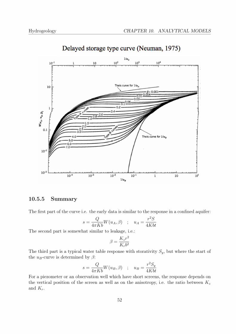
10.5.3 Drawdown and delayed storage, Neumann type curves

Initially rapid drawdown, after a while drawdown will almost stop. After a longer periodit starts again = Delayed storage type curve (note double log).

10.5.4 Early and late effects

The vertical conductivity is often lower because of lower grain size layers (drapings), whichmeans anisotropic conductivity. This means that for some time, drawdown from well doesnot reach the upper laying water table. The response will in the beginning lay on theelastic properties of the aquifer.

This means two u-values (early and late). Two Theis curves:

s =Q

4πTW (uA, uB, β)

For early data (elasticity):

1

uA=Tt

sr2

Late data (specific yield):

1

uB=

Tt

Syr2

β =Kzr

2

Krb2

Kz: Vertical hydraulic conductivity, Kr: Horizontal hydraulic conductivity.To determine the long-time effects a lot of testing and modeling is needed.

51


10.5.5 Summary

The first part of the curve i.e. the early data is similar to the response in a confined aquifer:

s =Q

4πKbW (uA, β) ; uA =

r2S

4KbtThe second part is somewhat similar to leakage, i.e.:

β =Kzr

2

Krb2

The third part is a typical water table response with storativity Sy, but where the start ofthe uB-curve is determined by β:

s =Q

4πKbW (uB, β) ; uB =

r2Sy4Kbt

For a piezometer or an observation well which have short screens, the response depends onthe vertical position of the screen as well as on the anisotropy, i.e. the ratio between Kz

and Kr.

52

Hydrogeology 10.6. SLUG TESTING AND STEPWISE TESTING, S&Z CH.12

10.6 Slug testing and stepwise testing, S&Z ch.12

A solid bar of iron is dropped into the well, that rises the water level in the well. Thisadditional head makes the water flow from the well into the aquifer. After equilibrium isreattained, the steel bar is rapidly lifted up. The lower hydraulic head in the well makesthe water flow into the well from the aquifer.This gives local, quick and cheap information about the aquifer.

The general solution for the hydraulic conductivity for a Hvorslev slug test is:

K =A

F

1

t2 − t1lnH1

H2

A: Cross sectional area of the wellH0: Initial water level (used for normalizing)H1 and H2: Water levels just after slug is placed/removed.F : Shape factor, see table 12.1 in textbook.

A common Hvorslev test where length L > 8R, where R is the radius of the piezometer:

F =2πL

ln(L/R)

⇒ K =R2 · ln(L/R)

2LT0

Where T0 is the time for which the rise of the water table is 37% of the initial column ofwater i.e. before removal of the slug.

With a confined aquifer a more advanced method is used (Cooper-Bredehoeft-Padadopulos).

10.7 Bounded aquifers

= Aquifer without infinite horizontal extent and isotropy.

Negative boundary: Impermeable limit zonePositive boundary: Boundary which can supply water. For example a stream, that isnot affected by loss of water into aquifer, because the discharge in a stream is much greater.

53


1) Semi infinite aquifer

2) Buried valley: When the drawdown reaches the valley sides, water must be supplied byvalley up- or downstream, because lateral extent is not infinite.

3) Strip aquifer

4) Strip aquifer

5) Infinite aquifer with positive boundary (stream). The hydraulic head can never bechanged at stream.

6) When left boundary (with lower K) is reached by drawdown, discharge drops.

10.7.1 Drawdown near positive boundary

The hydraulic head can never be changed at the positive boundary (fx stream). A fictionalrecharge well is placed symmetrically on the opposite side of the stream.

The recharge well will have the same recharge (| − Qw|) as the real well has discharge(| + Qw|). This will create constant head at stream location. No matter how big thedischarge at a well is, the system will be unaffected on the other side of a stream.

54

Hydrogeology 10.7. BOUNDED AQUIFERS

Pumping near stream:

s(r) =Qw

2πT

[lnr′

r

]=

Qw

4πTln

(x+ x0)2 + y2

(x− x0)2 + y2

55


Discharge from stream: The influence of the pumping well on the stream, i.e. howmuch water the stream loses by passing the well field. The ecosystem can be damaged bywell pumping near upstream areas.

The inflow from the stream at x=0 over a unit of length on y is integrated, and the specificdischarge is found. Q/Qq: Amount of water extracted from section of stream/y-axis inrelation to the total discharge from well.

Q

Qw

=2

πtan−1

(d

x0

)x0: (Shortest) distance between stream and welld: Length of stream (starting at midpoint)[tan−1]: rad

10.7.2 Drawdown near negative boundary

There can be no velocity components from boundary, since it acts as an impermeableboundary.

A fictional well is placed symmetrically opposite of the limit zone with respect to thereal well. The imaginary well will have the same discharge (+Qw) as the real well. Thesymmetrical nature creates a no-flow condition at the boundary exactly between the twowells ( δφ

δx= 0). The drawdown at the boundary will be twice the drawdown in an unlimited

aquifer.

56

Hydrogeology 10.7. BOUNDED AQUIFERS

r: Distance to observational well from real wellr’: Distance to observational well from imaginary wellărw: Radius of the well

The drawdown at the impermeable boundary r = r′:

s(r = r′) =Qw

πTlnr

rw

In real situations the radius of the well (rw), the value can be uncertain because of distur-bance of the formation while drilling (especially if the drilling happens with a wider bitthan the screen).

57


10.7.3 Pumping situations with multiple positive/negative bound-aries

The discharge/recharge has the same numerical value in each situation below. All situationsmust balance out in relation to the symmetry lines.

10.7.4 Well between two streams in infinite strip

When trying to balance this, an infinite amount of imaginary wells are placed at a longerand longer distance from the real well. There is a solution, see litterature (will not berequired at exam).

10.8 Well in uniform flow

Combination of natural flow and drawdown. The result is obtained by adding (superposi-tion). Constant flow: Linear hydraulic head.

All water within the groundwater divide will be flowing into the well.

58

Hydrogeology 10.8. WELL IN UNIFORM FLOW

Influx from regional flow q0, [m3/s per m2 = m/s]. Aquifer thickness: B, regional flow hashead 0. Stagnation point is examined (singular point).

Steady flow to well:

φQ =Qw

4πTln(x2 + y2)

Steady and isotropic flow. When two gradients are perpendicular:

δφ

δx=δψ

δy⇒

δφ

δx=q0B

T+

Qw

4πT

2x

x2 + y2=δψ

δy⇒

ψ =

∫q0B

Tdy +

Qw2x

4πT

∫1

x2 + y2dy ⇒

Ψ =q0B

Ty +

Qw

2πTtan−1

(yx

)At the divide: Ψ = 0

q0B

Ty = − Qw

2πTtan−1

(yx

)⇒ tan−1

(yx

)= −2πq0By

Qw

59


y

x= ±tan2πq0By

Qw

with + for y > 0, - for y < 0

Stagnation for: Ψ = 0 for y = 0

(xs, 0) =−Qw

2πq0B

10.9 Abstraction - long term influences, S&Z ch.8

See additional material: ’Noget om følgevirkninger af grundvandsindvinding’ by HenrikKjærgaard.

With groundwater extraction, the regional hydraulic pattern is changed. The groundwater-catchment can be altered.

60

Hydrogeology 10.9. ABSTRACTION - LONG TERM INFLUENCES, S&Z CH.8

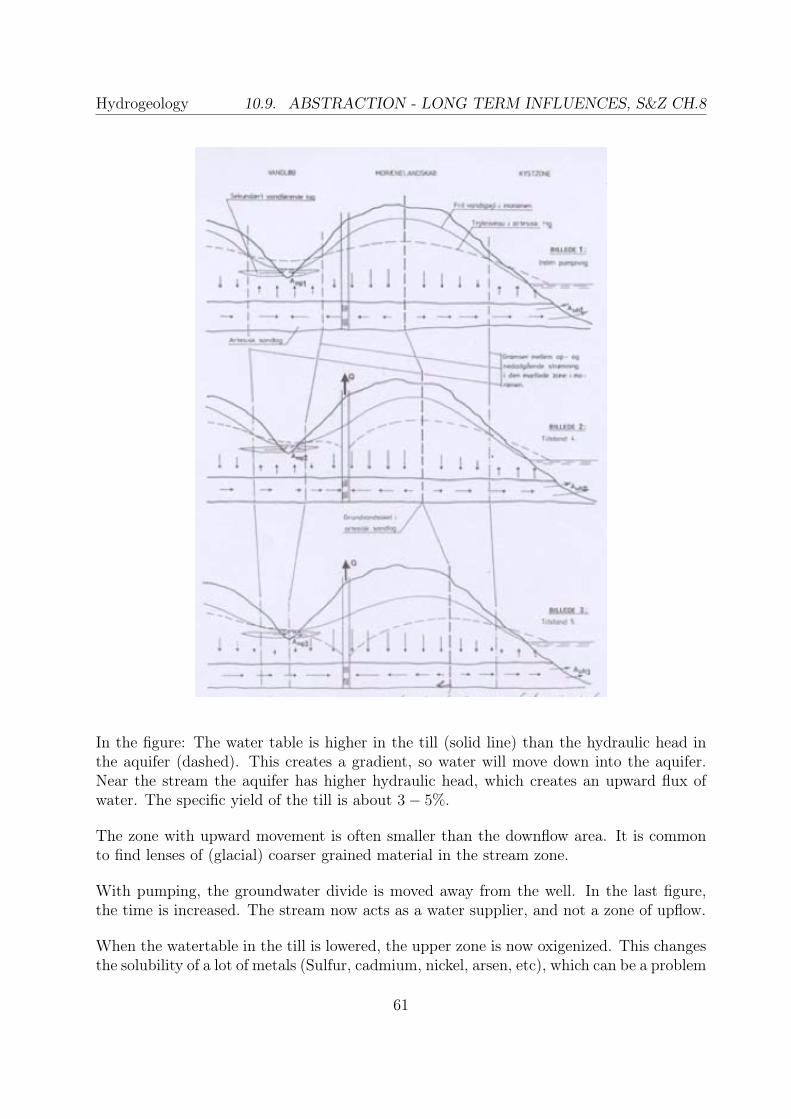
In the figure: The water table is higher in the till (solid line) than the hydraulic head inthe aquifer (dashed). This creates a gradient, so water will move down into the aquifer.Near the stream the aquifer has higher hydraulic head, which creates an upward flux ofwater. The specific yield of the till is about 3− 5%.

The zone with upward movement is often smaller than the downflow area. It is commonto find lenses of (glacial) coarser grained material in the stream zone.

With pumping, the groundwater divide is moved away from the well. In the last figure,the time is increased. The stream now acts as a water supplier, and not a zone of upflow.

When the watertable in the till is lowered, the upper zone is now oxigenized. This changesthe solubility of a lot of metals (Sulfur, cadmium, nickel, arsen, etc), which can be a problem

61


in dissolved state in the groundwater. The lowered hydraulic head in the aquifer increasesthe intergranular stress. This may lead to consolidation and lowering of the topographicsurface.

10.9.1 Release of water - initial phase

Release from aquifer, and additional release from aquitards.

62

Hydrogeology 10.10. SALT WATER INTRUSION

10.9.2 Release of water - late phase

The watertable starts to decline. The aquifer can over the long term not deliver unlimitedamounts of water.

Drawdown uses the entire storage capacity.

10.10 Salt water intrusion

Saltwater has higher density than fresh water. Hydraulic head:

φ = z +p

ρg, ρf < ρs

For obtaining equal pressure, a freshwater column is 4% higher than a saltwater column:

ρs = 1.04, ρf = 1.00 ⇒ hf = 1.04 · hs

63


If an aquifer contains saline water, the apparent hydraulic head (point water pressure head)looks lower. A salinity test will show, that the hydraulic head must be multiplied with afactor, to find the equivalent fresh-water head.

More: Ghyben - Herzberg equilibrium on interface; See slides. These formulas are simplifiedthough, as there is no seepage. Glover (1964) is a better approximation (note: x-directionopposite).

10.11 Stream groundwater interaction

Article by C.T. Jenkins

What happens to a stream on short term basis, not long term (steady state) as calculatedbefore.

Example: Full hydraulic contact through watertable aquifer. Stream is linear (line-source).The influence is integrated over stream length.

Parameters:

u =r2S

4Tt=sdf

4t

sdf =l2S

T

sdf : Stream depletion factor, dimensionless and constantq/Q : Dimensionless pumping rate, the amount of stream water pumped up by well.(1=100%)V/(Qt) : Dimensionless volume

64

Hydrogeology 10.11. STREAM GROUNDWATER INTERACTION

In the graph, 1− q/Q is added to make it possible to read more precise values.

First t/sdf is calculated, and then q/Q is found on curve A.

65

Appendix A

Hydrogeology terms

Aquifer: A geologic unit capable of supplying useable amounts of groundwater to a wellor spring. Classification of a water-bearing unit as an aquifer may depend upon localconditions and context of local water demands.

Aquitard: A bed or unit of lower permeability, that can store water but does not readilyyield water to pumping wells.

Cappilary fringe: The lowest part of the unsaturated zone in which the water in pores isunder pressure less than atmospheric, but the pores are fully saturated. This waterrises against the pull of gravity due to surface tension at the air-water interface andattraction between the liquid and solid phases.

Confined aquifer: An aquifer that is completely saturated and overlain by a confiningunit.

Darcy: A unit of permeability equal to 9.87 · 10−13m2, or for water of normal density andviscosity, a hydraulic condctivity of ∼ 10−5m

s

Drawdown (s): The difference between static water level (water table in unconfinedaquifers or potentiometric surface in confined aquifers), and pumping water levelin a well.

Effective porosity (ne): The percent of total volume of rock or soil that consists ofinterconnected porespaces, as used in describing groundwater flow and contaminanttransport.

Hydraulic conductivity (K): The proportionality constant in Darcy’s law – a measureof a porous medium’s ability to transmit water. K incorporates properties of boththe medium and fluid.

66

Hydrogeology

Hydraulic head (h): A measure of the potential energy of groundwater, it is the levelto which water in a well or piezometer will rise if unhindered. Total hydraulic headis the sum of two primary components: elevation head and pressure head. The thirdcomponent, velocity head, is generally negligible in groundwater.

Hydrostratigraphic unit: A formation, part of a formation, or group of formations withsufficiently similar hydrologic characteristics to allow grouping for descriptive pur-poses.

Permeability (k): A proportionality constant that measures a porous medium’s ability totransmit a fluid. It is a function of the medium’s physical properties. Permeability isdependent solely on properties of the porous medium, and is related to the hydraulicconductivity (K), the dynamic viscosity (µ) and the density of the fluid (ρ).

Perched groundwater: Unconfined groundwater separated from an underlying zone ofgroundwater by an unsaturated zone. This usually occurs atop lenses of clay orlow-permeability material above the groundwater table.

Porosity (n): The ratio of void space to total volume of a soil or rock.

Potentiometric surface: A surface constructed from measurements of head at individualwells of piezometers that defines the level to which water will rise from a single aquifer.

Saturated zone: The zone in which 100% of the porosity is filled with water.

Specific capacity: The yield of a well per unit of drawdown (s).

Specific retention (Sr): The volume of water that remains in a porous material aftercomplete drainage under the influence of gravity. Sr + Sy = n (total porosity)

Specific storage (Ss): The amount of water per unit volume of a saturated formationthat is stored or expelled per unit change of head due to the compressibility of thewater and aquifer skeleton.

Specific yield (Sy): The volume of water that drains under the influence of gravity froma porous material.

Static water level: The level to which water rises in a well or unconfined aquifer whenthe level is not influenced by pumping.

Storativity (S): The volume of water that a permeable unit releases from or takes intostorage per unit surface area per unit change in head. In unconfined aquifers it isequal to specific yield (Sy). The storativity in a confined aquifer is the product ofspecific storage (Ss) and the aquifer thickness (b).

Transmissivity (T ): A measure of the amount of water that can be transmitted horizon-tally through a unit width by the full saturated thickness of an aquifer. T is equalto the product of hydraulic conductivity (K) and saturated aquifer thickness (b).

67

Hydrogeology APPENDIX A. HYDROGEOLOGY TERMS

Unconfined aquifer: (alternate terms: phreatic- or watertable aquifer). An aquifer thatis only partially filled with water and in which the upper surface of the saturatedzone is free to rise and fall.

Unsaturated zone: The zone in which soil/sediment/rock porosity is filled partly withair and partly with water.

Water table: The top of the zone of saturation – the level at which the atmosphericpressure is equal to the hydraulic pressure. In unconfined aquifers the water table isrepresented by the measured water level in observation wells.

Well efficiency: The ratio of theoretical drawdawn (drawdown in the aquifer at the radiusof the well) to the observed drawdown inside a pumping well.

Well yield: The volume of water per unit of time discharged from a well by pumping orfree flow. It is commonly reported as a pumping rate (Q) in m3

s.

68

Appendix B

Commonly used formulas

B.1 Basic hydraulics in streams

Rectangular channelArea of the flow A = b · y [m2]Wetted perimeter P = b+ 2y [m]

Hydraulic radius R = byb+2y

[m]

Froudes number Fr = V√g·y [−]

Fr < 1: SubcriticalFr = 1: CriticalFr > 1: Supercritical

Gravitational acceleration g ≈ 9.81 m2

s

Critical depth (Fr = 1) yc = 3

√q2

g[m]

Specific energy E ≈ y + αQ2

2gA2 [J ]

Velocity coefficient α ≈ 1 [−]Manning number M = 25.4

6√k

[m1/3 · s−1]

M = Q

by( byb+2y

)2/3√S0

[m1/3 · s−1]

Velocity (M) V = M ·R2/3 ·√S0 [m

s]

Discharge(M) Q = A ·M ·R2/3 ·√S0 [m

3

s]

Discharge Q = A · V [m3

s]

Hydrostatic pressure distribution z + pγ

= h = constant [m]

Reynolds no. (< 580: Laminar, > 750: Turbulent) Re = V Rν

[−]

Kinematic viscosity (water, T = 20oC) ν = µρ

= 1 · 10−6 [m2

s]

Specific flow rate q = Q/b [m2

s]

69

Hydrogeology APPENDIX B. COMMONLY USED FORMULAS

Conservation lawsRate of change of mass ∆(ρA∆x)

∆t[kgs

]

Continuity equation* δAδt

+ δQδx

= 0Time t [s]Displacement in flow direction x [m]Momentum of a moving point p = mV [kg · m

s]

Conservation of momentum* 1gδVδt

+ VgδVδx

+ δyδx

+ Sf − S0 = 0

Longitudinal channel bottom slope S0 = sinθ [−]

Friction slope Sf =Ff

γA∆x

*) If the flow is steady (the flow conditions not varying with time), the partial derivativeterms with respect to time can be dropped from the continuity, momentum and energyequations. See page 18, Akan.

Loss in pipesInlet loss ∆HI = 0.5 Q2

2gA2 [m]

Pipe loss (friction) ∆HF = LM2R4/3A2 ·Q [m]

Outflow loss ∆Hu = αQ2

2gA2 [m]

Total loss See section 6.4 [m]

Hydraulic structures: See chapter 7.

B.2 Groundwater

The Darcy equation is valid for fully laminar flow in homogenous material.

Darcy’s equationHydraulic conductivity K = kρwg

µ[ms

]

Permeability k [m2]Dynamic viscosity (water, T = 20oC) µ = 1.002 · 10−3 [Pa · s]Hydraulic gradient i = − δh

δl= h2−h1

∆l[−]

Darcy’s equation q = Ki or Q = KiA [m2

s] or [m

3

s]

Transmissivity T = K · b [m2

s]

Storativity (assuming HPD) S = SsB [m2

m]

Specific storativity Ss [m3

m]

Porosity nT [−]

70

Hydrogeology B.2. GROUNDWATER

B.2.1 W(u) - Theis equation/Well function

W(u) is the Well function, that is called the exponential integral, E1, in non-hydrogeologyliterature. The value can be calculated with Matlab’s expint(u). A series of W (u) valuescan be looked up in table 9.2 (p. 225) in Schwarz & Zhang.

B.2.2 Unconfined aquifer: Steady 1D groundwater flow

When observing ground water elevation, the height (h) of the groundwater table is a goodexpression for the energy, because the velocity is relatively very small, and the pressure atthe groundwater table equals atmospheric pressure.

Condition: For expressing the flow as 1D flow (Dupuits approximation), the height varia-tions of the saturated zone must be less or equal than 10% the mean height of the saturatedzone:

∆hsath̄≤ 0.1

The problem: The amount of increase in specific discharge (dq = qout − qin) over a flowdistance (dx) is the supplied by seepage (W):

δq

δx= W , q = −T δh

δx

The differential equation for 1D flow in a homogeneous and isotropic aquifer:

⇒ δ

δx(q) = −T δ

2h

δx2= W

⇒ δ2h

δx2= −W

T⇒ δh

δx= −W

Tx+ c1

⇒ h = −W2T

x2 + c1x+ c2

By determining the boundary conditions, the constants can be found, thus solving thedifferential equation.

B.2.3 Confined aquifer: Steady 1D groundwater flow

A confined aquifer is totally filled by water under pressure. The piezometric surface (φ)is the corresponding water-pressure surface (groundwater-table in unconfined aquifer), ob-served in observation-drillings. Drainage lowers the pressure because of elastic storativity.

71

Hydrogeology APPENDIX B. COMMONLY USED FORMULAS

Lowering of the piezometric surface in a confined by drainage results in much less waterthan by lowering of the groundwater table in an unconfined aquifer.

The problem: The amount of increase in specific discharge (dq = qout − qin) over a flowdistance (dx) is the supplied by seepage (W):

δq

δx= W , q = −T δφ

δx

The flow equation is derived by the principles of conservation of mass, the Darcy equation,elastic properties and elastic laws. The differential equation for 1D flow in a homogeneousand isotropic aquifer:

⇒ δ

δx(q) = −T δ

2φ

δx2= W

⇒ δ2φ

δx2= −W

T⇒ δφ

δx= −W

Tx+ c1

⇒ φ = −W2T

x2 + c1x+ c2

By determining the boundary conditions, the constants can be found, thus solving thedifferential equation.

B.2.4 Boundary conditions

The most often used boundary conditions:

• Known hydraulic head - Dirichlet BVP:φ = φ2(x, y, z, t) or h = h2(x, y, z, t), example: a large lake, a stream, the sea.

• Known flux - Neuman BVP:Example: Impermeable material or groundwater divide: No flow at boundary: q = 0and δφ

δx= 0 or δh

δx= 0.

h is used for unconfined/phreatic/watertable aquifers, φ for confined aquifers.

72

Notes for ’Hydrogeology’ - Anders Damsgaard · Notes for ’Hydrogeology’ Anders Damsgaard...

Documents

Transcript of Notes for ’Hydrogeology’ - Anders Damsgaard · Notes for ’Hydrogeology’ Anders Damsgaard...